The NPT Ensemble Explained: From Theory to Application in Drug Discovery and Biomolecular Simulation

Abstract

This article provides a comprehensive exploration of the isothermal-isobaric (NPT) ensemble, a cornerstone of statistical mechanics and molecular simulation. Tailored for researchers and drug development professionals, it details the ensemble's foundational theory, its practical implementation via modern algorithms and barostats, and strategies for troubleshooting common issues. Highlighting a 2025 case study, the article demonstrates how NPT simulations, when combined with machine learning, are used to predict critical drug properties like aqueous solubility, validating the ensemble's pivotal role in advancing biomedical research.

Understanding the NPT Ensemble: Statistical Mechanics and Thermodynamic Foundations

The isothermal-isobaric ensemble, almost universally referred to as the NPT ensemble, is a foundational concept in statistical mechanics and computational physics. It describes a thermodynamic system in contact with a surrounding environment that maintains constant particle number (N), constant pressure (P), and constant temperature (T) [1] [2]. This ensemble represents a system that can exchange both energy and volume with its surroundings, thereby existing in simultaneous thermal and mechanical equilibrium with a heat bath and a pressure reservoir [3]. The NPT ensemble is exceptionally valuable because it closely mirrors a vast array of real-world experimental conditions, particularly in chemistry and materials science, where reactions and processes often occur at atmospheric pressure and controlled temperature [2] [3].

Within the framework of statistical mechanics, the NPT ensemble connects the microscopic properties of a system to its macroscopic observables through statistical averages [3]. The characteristic thermodynamic potential for this ensemble is the Gibbs free energy (G), which is minimized when the system reaches equilibrium [1] [3]. The ability to study systems under constant N, P, and T conditions makes this ensemble indispensable for investigating phase transitions, material compressibility, and the properties of liquids, polymers, and biological macromolecules [1] [3].

Theoretical Foundations

The Partition Function and Probability Distribution

The partition function serves as the cornerstone of any statistical ensemble, encapsulating all its thermodynamic properties. For the NPT ensemble, the partition function, denoted as Δ(N, P, T), is derived from the canonical (NVT) partition function by introducing volume as an additional variable and incorporating the pressure-volume work term [1] [3].

For a classical system, the NPT partition function can be expressed as: Δ(N, P, T) = ∫ e^(-βPV) Z(N, V, T) C dV [1]

Here:

• β = 1/(k_B T), where k_B is the Boltzmann constant.
• P is the external pressure.
• V is the volume of the system.
• Z(N, V, T) is the canonical (NVT) partition function.
• C is a constant ensuring the partition function is dimensionless [1].

An alternative formulation sums over all possible microstates i of the system. The probability p_i of finding the system in a specific microstate i with energy E_i and volume V_i is given by the generalized Boltzmann distribution: p_i = Z^{-1} e^{-β(E_i + PV_i)} [1]

In this equation, Z acts as the normalization constant. This probability distribution highlights that the likelihood of a microstate depends on both its energy and its volume, weighted by the external pressure.

Connection to Thermodynamics: Gibbs Free Energy

The bridge between the microscopic description of the NPT ensemble and macroscopic thermodynamics is the Gibbs free energy (G). It is calculated directly from the partition function [1] [3]: G(N, P, T) = -k_B T ln Δ(N, P, T)

The Gibbs free energy is the relevant thermodynamic potential for processes occurring at constant pressure and temperature. The equilibrium state of a system under these conditions is determined by the minimization of G. This fundamental connection allows for the calculation of all other thermodynamic quantities through derivatives of G or the partition function [3].

Table 1: Key Thermodynamic Relationships in the NPT Ensemble

Thermodynamic Quantity	Relation to Partition Function or Averages
Gibbs Free Energy (G)	G = -k_B T ln Δ(N, P, T) [1] [3]
Average Energy (⟨E⟩)	⟨E⟩ = - (∂ ln Δ / ∂ β)_{N, P}
Average Volume (⟨V⟩)	⟨V⟩ = - (1/β) (∂ ln Δ / ∂ P)_{N, T} [3]
Enthalpy (H)	H = ⟨E⟩ + P⟨V⟩ [3]
Entropy (S)	S = - (∂ G / ∂ T)_{N, P} [3]

Fluctuations and Response Functions

In the NPT ensemble, both the energy and the volume are fluctuating quantities. The magnitude of these fluctuations is not arbitrary; it is intrinsically linked to the system's fundamental response functions. The variance of the volume fluctuations, for instance, is proportional to the isothermal compressibility, κ_T, which measures how much a material compresses under pressure at constant temperature [3]: κ_T = - (1/⟨V⟩) (∂⟨V⟩/∂P)_T = (⟨V²⟩ - ⟨V⟩²) / (k_B T ⟨V⟩)

Similarly, energy fluctuations are related to the system's heat capacity. These relationships demonstrate how measurable material properties emerge from the statistical nature of molecular motions and configurations.

Practical Implementation in Computer Simulations

Molecular Dynamics with Thermostats and Barostats

In Molecular Dynamics (MD) simulations, the NPT ensemble is generated by applying algorithms that control both temperature and pressure. This requires the combined use of a thermostat and a barostat [4] [5].

Thermostats maintain a constant temperature by adjusting the atomic velocities. Common algorithms include:

• Nosé-Hoover Thermostat: An extended system method that introduces an additional degree of freedom to represent the heat bath, generating a correct canonical distribution [6] [5].
• Berendsen Thermostat: A weak-coupling method that scales velocities to gently drive the temperature towards the target value. It is efficient but does not produce a strictly rigorous ensemble [4].
• Langevin Thermostat: Applies stochastic and friction forces to particles to maintain temperature, often used in conjunction with barostats like Parinello-Rahman [7].

Barostats maintain constant pressure by dynamically adjusting the simulation cell's volume or shape. Key algorithms include:

• Parrinello-Rahman Barostat: An extended system method that allows for fully flexible simulation cells, enabling the study of solid-state phase transitions where the cell shape may change. It is considered one of the most robust and versatile barostats [7] [5].
• Berendsen Barostat: Scales the cell dimensions to gradually relax the internal pressure to the target pressure. Like its thermostat counterpart, it is efficient for equilibration but does not generate the exact NPT ensemble [5].

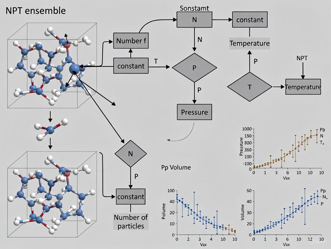
The following diagram illustrates the workflow of an NPT-MD simulation, integrating these core components:

Monte Carlo Methods

In Monte Carlo (MC) simulations, the NPT ensemble is sampled through random moves. In addition to the particle displacement moves used in the NVT ensemble, NPT Monte Carlo incorporates volume change moves [3] [8]. A trial move involves randomly changing the volume of the simulation box and uniformly scaling the coordinates of all particles within it. This trial move is then accepted or rejected based on a criterion that ensures the system samples configurations according to the correct NPT probability distribution, which includes the e^(-β P ΔV) term from the partition function [8]. This method is particularly powerful for studying phase equilibria and calculating free energy differences.

Experimental Protocols and Research Applications

A Representative Workflow: Epoxy Network Mechanics

A study on the elastic properties of elastomeric epoxy networks provides an excellent example of a detailed NPT-MD protocol [6]. The research investigated stoichiometric networks formed from poly(ethylene glycol) diglycidyl ether (PEGDE) and 1,4-diaminobutane (DAB).

Table 2: Key Reagents and Computational Tools for Epoxy Network Simulation

Research Reagent / Tool	Function / Description
Poly(ethylene glycol) diglycidyl ether (PEGDE)	Bifunctional epoxy precursor that forms the network backbone.
1,4-diaminobutane (DAB, Putrescine)	Tetrafunctional cross-linker; amine groups react with epoxy groups.
PCFF-IFF Force Field	An interatomic potential providing parameters for polymers, used to calculate energies and forces.
LAMMPS (Large-scale Atomic/Molecular Massively Parallel Simulator)	Open-source MD software used to perform the energy minimization, equilibration, and production runs.
LUNAR	Open-source Python code used for system configuration, file preparation, and force field application.
Nosé-Hoover Thermostat & Barostat	Algorithms used to maintain constant temperature (27°C) and pressure (1 atm) during the NPT equilibration phase.

Detailed Protocol [6]:

• System Preparation: PEGDE and DAB molecules were packed into a low-density simulation box (0.2 g/cm³).
• Energy Minimization: The conjugate-gradient method was used to relax the system and find a local energy minimum.
• NPT Equilibration: The system was equilibrated in the NPT ensemble at 27°C and 1 atm for 500 ps using a Nosé-Hoover thermostat and barostat with a 1 fs time step.
• Densification: The simulation box volume was gradually reduced over 5 ns to reach the target bulk density of ~1.11 g/cm³.
• Annealing: The system underwent a thermal annealing cycle (heating to 227°C and cooling back to 27°C) to enhance relaxation.
• Cross-linking: Epoxide-amine cross-linking reactions were simulated using the REACTER protocol in LAMMPS until a specific reaction extent (~82% or ~92.5%) was achieved.
• Final Equilibration: The newly formed network was equilibrated again in the NPT ensemble for 100 ns at 27°C and 1 atm.
• Mechanical Characterization: The equilibrated network was subjected to uniaxial tensile and shear deformations at various high strain rates (10⁷ to 10¹⁰ s⁻¹) under the NPT ensemble to calculate Young's modulus and other elastic constants.

Case Study: Negative Thermal Expansion in ScF₃

The NPT ensemble is crucial for studying unusual material properties, such as negative thermal expansion (NTE). Ab initio MD simulations in the NpT ensemble were used to investigate the lattice contraction of scandium fluoride (ScF₃) upon heating [9]. The simulations were performed at temperatures from 300 K to 1600 K. A key finding was the sensitivity of the results to the size of the simulation supercell; a supercell larger than 2a×2a×2a was required to accurately capture the dynamic disorder responsible for the NTE effect. The study concluded that the NTE in ScF₃ arises from the interplay between the expansion of Sc-F bonds and the rotation of ScF₆ octahedra, a mechanism that could only be elucidated through the volume-fluctuating NPT ensemble [9].

Calculation of Thermal Expansion Coefficients

A common application of NPT-MD is the calculation of the coefficient of thermal expansion for solids. A typical protocol, as demonstrated for fcc-Cu, involves [5]:

• Running a series of NPT simulations at different target temperatures (e.g., from 200 K to 1000 K in 100 K increments).
• For each temperature, allowing the system to equilibrate fully and then sampling the average lattice constant over a production run.
• Plotting the average lattice constant or volume as a function of temperature.
• The thermal expansion coefficient is then derived from the slope of this curve. This requires careful parameterization of the barostat, such as selecting an appropriate pfactor (related to the barostat's time constant and the system's bulk modulus) in the Parrinello-Rahman method [5].

Comparison with Other Statistical Ensembles

The NPT ensemble is one of several used in statistical mechanics and simulation, each suited to different physical conditions.

Table 3: Comparison of Common Statistical Ensembles

Ensemble	Fixed Variables	Fluctuating Quantities	Common Applications
NVE (Microcanonical)	Number (N), Volume (V), Energy (E)	Temperature, Pressure	Fundamental MD; study of isolated systems.
NVT (Canonical)	Number (N), Volume (V), Temperature (T)	Energy, Pressure	Simulating systems in a heat bath with fixed boundaries.
NPT (Isothermal-Isobaric)	Number (N), Pressure (P), Temperature (T)	Energy, Volume	Real-world lab conditions; studying density, phase transitions.
μVT (Grand Canonical)	Chemical Potential (μ), Volume (V), Temperature (T)	Energy, Particle Number (N)	Open systems; adsorption, phase equilibria.

The NPT ensemble is often preferred over NVT for modeling realistic experimental conditions where pressure, not volume, is controlled. It is distinct from the grand canonical (μVT) ensemble, which allows particle exchange and is better suited for studying open systems [3].

Based on the protocols and studies cited, successful implementation of the NPT ensemble in research relies on a combination of software, algorithms, and physical models.

Table 4: Essential Tools for NPT Ensemble Research

Tool / Reagent	Category	Specific Examples	Function
Simulation Software	Software	LAMMPS [6], VASP [7], CP2K [9], ASE [5]	Core platforms for performing MD or MC simulations.
Thermostat Algorithms	Algorithm	Nosé-Hoover [6] [5], Berendsen [4] [5], Langevin [7]	Controls and stabilizes the simulation temperature.
Barostat Algorithms	Algorithm	Parrinello-Rahman [7] [5], Berendsen [5]	Controls and stabilizes the simulation pressure.
Interatomic Potentials	Model/Force Field	PCFF-IFF (for polymers) [6], EMT (for metals) [5], DFT (for ab initio) [9]	Describes the interactions between atoms, the core of the energy calculation.
System Builder Tools	Software	LUNAR [6], ASE.build [5]	Prepares initial atomic configurations and simulation cells.
Analysis Tools	Software	In-house scripts, visualization software (e.g., OVITO, VMD)	Processes simulation trajectories to compute properties like RDF, stress, etc.

The NPT ensemble provides an indispensable framework for bridging the microscopic world of atoms and molecules with the macroscopic thermodynamic behavior of systems at constant pressure and temperature. Its theoretical foundation in statistical mechanics is robust, centered on the Gibbs free energy and a partition function that accounts for volume fluctuations. From a practical standpoint, the implementation of the NPT ensemble in molecular dynamics and Monte Carlo simulations via thermostats and barostats allows researchers to accurately model realistic conditions. As demonstrated by its applications in predicting material properties like the elasticity of polymer networks and the anomalous negative thermal expansion in ScF₃, the NPT ensemble remains a cornerstone technique for advancing research in drug development, materials science, and chemical physics.

The isothermal-isobaric (NPT) ensemble is a cornerstone of statistical mechanics, providing the essential theoretical framework for understanding systems that exchange both energy and volume with their surroundings at constant temperature (T), pressure (P), and particle number (N). This ensemble mirrors countless real-world experimental conditions, from chemical reactions at atmospheric pressure to the physiological environment of biological systems [3]. Its power lies in connecting the microscopic details of molecular interactions to macroscopic thermodynamic observables, enabling the prediction of material properties, phase behavior, and reaction equilibria.

This technical guide delineates the statistical mechanical basis of the NPT ensemble, beginning with a formal derivation of its partition function. We will establish the connection between this partition function and the Gibbs free energy, the characteristic thermodynamic potential for the ensemble. Furthermore, the document will explore the theoretical underpinnings of fluctuations and response functions, and conclude with a discussion on the practical implementation of NPT ensemble in modern computational methods, providing detailed protocols for molecular dynamics simulations.

Theoretical Foundation and Derivation

The NPT ensemble describes a system in simultaneous thermal and mechanical equilibrium with its environment. The derivation of its partition function can be approached from multiple angles, each illuminating a different aspect of the ensemble's statistical nature.

The System-and-Bath Derivation

A physically intuitive derivation involves considering a system of interest coupled to a much larger bath that acts as both a heat and a pressure reservoir [1]. The system has a fixed number of particles N, but its volume V can fluctuate. The bath, with volume V₀ and a vastly greater number of particles M (where M - N >> N), is characterized by constant temperature T and pressure P.

The total partition function for the combined system (sys) and bath is given by: Z^sys+bath(N, V, T) = Z^sys(N, V, T) × Z^bath(M-N, V₀-V, T)

Assuming the bath is an ideal gas, its partition function is proportional to (V₀ - V)^M-N. In the thermodynamic limit (V₀ → ∞, M → ∞, with (M-N)/V₀ = ρ constant), the dependence on the system's volume V can be isolated. Using the ideal gas law, the particle density ρ is equivalent to βP, leading to the probability density for the system to be in a microstate with volume V and coordinates s^N being proportional to exp[-β( U(s^N) + PV )] [1].

Integrating over all possible volumes and microstates yields the isothermal-isobaric partition function, Δ(N, P, T): Δ(N, P, T) = ∫ dV e^{-βPV} Z(N, V, T) (1) where Z(N, V, T) is the canonical partition function [1] [3]. The pre-factor C in the integral (C dV) is a matter of convention; it can be set to βP or 1, with the latter being more common in modern treatments [1].

The Laplace Transform and Legendre Transform Relationship

Equation (1) reveals that the NPT partition function is the Laplace transform of the canonical partition function with respect to volume [10] [1]. This mathematical structure directly facilitates the Legendre transform that connects the Helmholtz free energy F(N, V, T) = -k_BT ln Z(N, V, T) to the Gibbs free energy G(N, P, T) in the thermodynamic limit.

The saddle-point approximation of the Laplace transform integral shows that in the thermodynamic limit (N → ∞), the primary contribution to the integral comes from the most probable volume, ⟨V⟩. This establishes the connection: G(N, P, T) = -k_BT ln Δ(N, P, T) (2) which is the fundamental thermodynamic relationship for the NPT ensemble [1] [11] [3]. The Gibbs free energy G is the characteristic state function for variables N, P, and T, and its minimization determines the equilibrium state of the system.

Table 1: Key Partition Functions and their Corresponding Thermodynamic Potentials

Ensemble	Partition Function	Thermodynamic Potential	Fundamental Relation
Microcanonical (NVE)	Ω(N, V, E) = eS(N,V,E)/kB	Entropy (S)	dE = TdS - PdV + μdN
Canonical (NVT)	Z(N, V, T) = ∫ dE Ω e^{-βE}	Helmholtz Free Energy (F)	F = E - TS
Isothermal-Isobaric (NPT)	Δ(N, P, T) = ∫ dV Z e^{-βPV}	Gibbs Free Energy (G)	G = F + PV = H - TS

Thermodynamic Quantities and Fluctuations

The NPT partition function serves as a generating function for all thermodynamic properties. The ensemble averages of energy and volume are given by: ⟨E⟩ = - ( ∂ ln Δ / ∂β )_P,N ⟨V⟩ = k_BT ( ∂ ln Δ / ∂P )_T,N

Furthermore, the Gibbs entropy formula for the NPT ensemble is: S = k_Bβ ⟨E⟩ + k_BβP ⟨V⟩ + k_B ln Δ(P, N, β) (3) which confirms that the NPT distribution is the one of maximum entropy for a given average energy and average volume [11].

A key feature of the NPT ensemble is the presence of natural fluctuations in energy and volume. These fluctuations are not mere noise but are quantitatively linked to the system's response functions. The isothermal compressibility, κ_T, which measures the relative volume change with pressure at constant temperature, is directly related to the variance of volume fluctuations [3]: κ_T = - (1/⟨V⟩) (∂⟨V⟩/∂P)_T = ( ⟨V²⟩ - ⟨V⟩² ) / ( k_BT ⟨V⟩ ) (4)

Similarly, the constant-pressure heat capacity, C_P, is related to the fluctuations in the enthalpy, H = E + PV [11]: C_P = ( ∂H/∂T )_P = [ ⟨(H - ⟨H⟩)²⟩ ] / ( k_BT² )

Table 2: Fluctuation-Response Relations in the NPT Ensemble

Fluctuating Quantity	Statistical Expression for Fluctuations	Related Thermodynamic Response Function
Volume (V)	⟨(δV)²⟩ = ⟨V²⟩ - ⟨V⟩²	Isothermal Compressibility: κT = ⟨(δV)²⟩ / (kBT ⟨V⟩)
Enthalpy (H = E+PV)	⟨(δH)²⟩ = ⟨H²⟩ - ⟨H⟩²	Constant-Pressure Heat Capacity: CP = ⟨(δH)²⟩ / (kBT²)

Computational Implementation and Protocols

The theoretical framework of the NPT ensemble is realized in computer simulations through Molecular Dynamics (MD) and Monte Carlo (MC) methods, enabling the atomistic study of materials under realistic conditions.

Molecular Dynamics and Barostat Algorithms

In MD, the NPT ensemble is generated by coupling the system to a thermostat and a barostat. The barostat dynamically adjusts the simulation cell's size and/or shape to maintain a constant internal pressure. Several barostat algorithms are commonly used [12] [5]:

• Berendsen Barostat: Scales the volume and coordinates with a first-order rate equation towards the target pressure. It is robust and efficient for equilibration but does not generate a rigorously correct NPT ensemble [12].
• Parrinello-Rahman Barostat: An extended system method that introduces additional dynamical variables for the simulation cell. It allows for fully flexible simulation boxes and correctly samples the NPT ensemble, making it suitable for studying solid-state phase transitions [5].
• Martyna-Tobias-Klein (MTK) Barostat: The Hamiltonian version of the Parrinello-Rahman method, also generating a correct NPT ensemble [12].
• Stochastic Barostats (e.g., Bernetti-Bussi): Stochastic variants that provide correct sampling even for very small unit cells and are often recommended for production simulations [12].

The following diagram illustrates the logical workflow and key components of an NPT molecular dynamics simulation.

Diagram 1: NPT-MD simulation workflow.

Detailed Protocol: NPT-MD Simulation with the Parrinello-Rahman Method

This protocol outlines the steps for performing an NPT-MD simulation to calculate the thermal expansion of a solid, such as a 3x3x3 supercell of fcc-Cu [5].

• System Setup:

  • Construct the initial crystal structure. For isotropic solids (e.g., cubic crystals), use isotropic pressure control.
  • Define the empirical or first-principles calculator (e.g., EMT, PFP, DFT).

• Parameter Initialization:

  • Time Step: Set to 1.0 fs for systems with light atoms or high frequencies.
  • Temperature: Set the target temperature (e.g., 300 K).
  • Pressure: Set the external pressure (e.g., 1 bar = 10⁻⁴ GPa).
  • Thermostat: Use a Nosé-Hoover thermostat with a time constant (τ_T or ttime) of ~20-100 fs.
  • Barostat: Use the Parrinello-Rahman method. The key parameter is pfactor (e.g., 2×10⁶ GPa·fs² for metals), which is related to the barostat time constant and the system's bulk modulus.

• Equilibration:

  • Initialize atomic velocities from a Maxwell-Boltzmann distribution at the target temperature.
  • Run the simulation for a sufficient number of steps (e.g., 20,000 steps for 20 ps) until the potential energy, temperature, and volume (or density) reach a stable plateau.

• Production and Analysis:

  • Continue the simulation, saving the trajectory at regular intervals.
  • Calculate the equilibrium volume ⟨V⟩ as a time average over the production phase.
  • To compute the thermal expansion coefficient, repeat the simulation and analysis at different temperatures.

Table 3: Research Reagent Solutions for Computational NPT Studies

Item / Software	Type / Function	Key Feature
LAMMPS	Molecular Dynamics Package	Highly versatile, supports many barostats and force fields.
GROMACS	Molecular Dynamics Package	Extremely fast for biomolecular systems.
QuantumATK	MD & Multi-scale Simulator	Integrates DFT with MD, user-friendly NPT setup.
ASE (Atomic Simulation Environment)	Python Library	Provides framework for defining and running NPT simulations with various calculators.
Parrinello-Rahman Barostat	Algorithm	Correctly samples NPT ensemble with a flexible cell.
Bernetti-Bussi Barostat	Algorithm	Stochastic barostat for correct NPT sampling in small cells.
PLUMED	Library	Enhanced sampling and analysis of MD trajectories, works with major MD engines.

The NPT partition function, Δ(N, P, T), provides the complete statistical mechanical description of a system at constant particle number, pressure, and temperature. Its derivation as a Laplace transform of the canonical partition function formally introduces pressure as a control variable and establishes the Gibbs free energy as the relevant thermodynamic potential. The formalism naturally accounts for volume and enthalpy fluctuations, linking them directly to fundamental material properties like compressibility and heat capacity. The transition of this theoretical framework from abstract mathematics to practical tool, through sophisticated computational algorithms like the Parrinello-Rahman barostat, has made the NPT ensemble indispensable for simulating and predicting the behavior of materials and biomolecules under realistic, constant-pressure conditions.

The isothermal-isobaric (NPT) ensemble is a cornerstone of statistical mechanics, providing the essential framework for modeling systems under constant temperature (T), pressure (P), and number of particles (N)—conditions that mirror most laboratory experiments and natural phenomena. Within this ensemble, the Gibbs free energy (G) emerges as the fundamental thermodynamic potential, serving as a bridge between the microscopic interactions of particles and the macroscopic thermodynamic properties we observe [11]. This whitepaper provides an in-depth technical examination of the NPT ensemble, detailing how Gibbs free energy is derived from, and fundamentally governs, this ensemble. It further explores modern computational methodologies for its calculation, supported by structured data, experimental protocols, and visualization tools tailored for researchers and drug development professionals.

The critical role of Gibbs free energy extends across scientific disciplines. In materials science, it determines phase stability and guides the design of new alloys [13]. In drug discovery, accurate prediction of binding affinities—a process governed by free energy changes—is paramount for optimizing lead compounds [14]. The NPT ensemble is the natural environment for these studies, and mastering its connection to Gibbs free energy is essential for advancing research in these fields.

Theoretical Foundations of the NPT Ensemble

Definition and Partition Function

The NPT ensemble describes a system in contact with both a thermal bath, maintaining constant temperature, and a mechanical piston, maintaining constant pressure. The ensemble is defined by its partition function, which for a classical system is given by Eq. (73) in [11]: [ \Delta(P, N, \beta) = \int dV \int d^{6N}\Gamma \exp\left{-\beta\left[H(\mathbf{p}^N, \mathbf{q}^N; V) + PV\right]\right} ] Here, ( \beta = 1/k_B T ), ( H ) is the system Hamiltonian, ( V ) is the system volume, and the integral is taken over the entire phase space of the system [11]. The partition function ( \Delta ) is the cornerstone from which all thermodynamic properties of the ensemble are derived. For quantum systems, the partition function involves a trace over quantum states and an integral over volume [11]: [ \Delta(P, N, \beta) = \int dV \, \text{Tr} \exp\left{-\beta\left[\hat{H}(V) + PV\right]\right} ] where ( \hat{H}(V) ) is the quantum Hamiltonian operator.

The Gibbs Free Energy as the Characteristic State Function

The Gibbs free energy, G, is the thermodynamic characteristic function for the variables N, P, and T. It is directly connected to the NPT partition function by [11] [1]: [ G(N, P, T) = -kB T \ln \Delta(N, P, T) ] This relationship is of profound importance because it implies that if the partition function ( \Delta ) is known, all other thermodynamic properties can be calculated by taking appropriate derivatives of G. The fundamental thermodynamic relation for G is [11]: [ dG = -S dT + V dP + \suml \mul dNl ] From this, the entropy (S), volume (V), and chemical potential (( \mul )) can be obtained as conjugate variables: [ S = -\left(\frac{\partial G}{\partial T}\right){P, N}, \quad V = \left(\frac{\partial G}{\partial P}\right){T, N}, \quad \mul = \left(\frac{\partial G}{\partial Nl}\right){T, P, N'} ]

Table 1: Key Thermodynamic Relations in the NPT Ensemble

Thermodynamic Property	Statistical Mechanical Relation	Reference Equation
Gibbs Free Energy, G	( G = -k_B T \ln \Delta(P, N, \beta) )	[11] Eq. (81)
Entropy, S	( S = kB T \frac{\partial \ln \Delta}{\partial T} + kB \ln \Delta )	[11] Eq. (86)
Average Volume, 〈V〉	( \langle V \rangle = -k_B T \frac{\partial \ln \Delta}{\partial P} )	[11] Eq. (87)
Enthalpy, H	( H = -\frac{\partial \ln \Delta}{\partial \beta} )	[11] Eq. (89)
Constant-Pressure Heat Capacity, C_P	( CP = kB \beta^2 \langle [(\mathcal{H}+PV) - \langle \mathcal{H}+PV \rangle]^2 \rangle )	[11] Eq. (91a)

Fluctuations and Their Physical Significance

In the NPT ensemble, thermodynamic quantities are not fixed but fluctuate around their mean values. These fluctuations are not mere noise; they are directly related to the system's thermodynamic response functions. A key example is the fluctuation in the enthalpy-like quantity ( \mathcal{H} + PV ), which is connected to the constant-pressure heat capacity, ( C_P ) [11]: [ \langle [(\mathcal{H}+PV) - \langle \mathcal{H}+PV \rangle]^2 \rangle = \frac{\partial^2 \ln \Delta}{\partial \beta^2} = - \frac{\partial \langle \mathcal{H}+PV \rangle}{\partial \beta} ] This result demonstrates that the heat capacity, a measurable macroscopic property, is fundamentally a measure of energy fluctuations within the system.

Computational Methodologies for the NPT Ensemble

Simulating the NPT ensemble requires algorithms that faithfully generate system configurations distributed according to the NPT probability density. The following diagram illustrates the logical relationship between the core theoretical concept (Gibbs Free Energy) and the primary computational methods used to sample the NPT ensemble.

Diagram 1: From Gibbs Energy to Computational Methods. This diagram outlines how the foundational concept of Gibbs Free Energy gives rise to the NPT partition function and the probability of microstates, which in turn dictates the design of major Monte Carlo and Molecular Dynamics sampling algorithms.

Monte Carlo Methods

Monte Carlo (MC) methods are a primary tool for sampling the NPT ensemble. They work by generating a Markov chain of system states (particle coordinates and system volume) where each new state is proposed randomly and accepted with a probability that ensures convergence to the correct NPT distribution [15]. The key acceptance criterion is based on the change in the effective energy ( Ei + PVi ).

A powerful variant is the Gibbs Ensemble Monte Carlo (GEMC), which is particularly efficient for simulating phase equilibria without an interface. In GEMC, two simulation boxes (e.g., representing vapor and liquid phases) are simulated in parallel, allowing for particle exchange and volume changes that equalize pressure and chemical potential between the boxes [16].

Molecular Dynamics Methods

Molecular Dynamics (MD) simulates the system by numerically solving Newton's equations of motion, modified to maintain constant temperature and pressure. This is typically achieved using extended Lagrangian formalisms, which introduce additional dynamical variables to represent the thermostat and barostat.

Recent algorithmic advances focus on improving the stability and sampling efficiency of NPT simulations. For instance, Li & Peng (2025) proposed a second-order Langevin sampler that preserves a positive volume for the simulation box [17]. Their method derives equations of motion by sending the artificial mass of the periodic box to zero, resulting in a system that guarantees the positivity of the volume and allows for the development of high-performance weak numerical schemes.

Table 2: Key Computational Methods for NPT Ensemble Sampling

Method Type	Specific Algorithm	Key Feature	Typical Application
Monte Carlo	Standard NPT MC	Volume change moves	General purpose NPT simulation [1] [15]
Monte Carlo	Gibbs Ensemble MC (GEMC)	Simulates two coexisting phases without an interface	Vapor-liquid equilibrium [16]
Molecular Dynamics	Nosé-Hoover / Parrinello-Rahman	Extended system with coupled thermostat/barostat	General purpose NPT MD [15]
Molecular Dynamics	2nd-Order Langevin Sampler	Positivity-preserving volume dynamics	Robust NPT sampling for small systems [17]

Experimental and Computational Protocols

Protocol 1: Calculating Phase Diagrams for Alloys using MLIPs

Predicting phase stability in complex alloys like high-entropy alloys (HEAs) is a critical application of NPT thermodynamics. The following workflow, as implemented in tools like PhaseForge, integrates machine learning interatomic potentials (MLIPs) for efficient and accurate phase diagram calculation [13].

Diagram 2: Workflow for Alloy Phase Diagram Calculation. This protocol shows the steps for constructing a phase diagram using Machine Learning Interatomic Potentials (MLIPs), from generating representative atomic structures to the final thermodynamic modeling and benchmarking.

Detailed Methodology [13]:

• Structure Generation: Generate Special Quasirandom Structures (SQS) for various phases (e.g., FCC, BCC, HCP) and compositions using a tool like the Alloy Theoretic Automated Toolkit (ATAT). SQS are periodic structures that best mimic the randomness of a true solid solution.
• Energy Calculation: Optimize the SQS structures and calculate their energy at 0 K using a trained MLIP (e.g., Grace, SevenNet, CHGNet). This provides the configurational energy of the ordered phases.
• Liquid Phase Handling: Perform NPT-MD simulations on the liquid phase at different compositions. The free energy of the liquid is often calculated using a "ternary search" method to integrate the thermodynamic relations.
• Thermodynamic Modeling: Fit all the calculated energies (for solid and liquid phases) using CALPHAD (CALculation of PHAse Diagrams) modeling within ATAT. This involves finding polynomial expressions for the Gibbs free energy of each phase as a function of composition and temperature.
• Diagram Construction: Construct the final phase diagram using CALPHAD software (e.g., Pandat), which calculates the phase equilibria by finding the global minimum of the total Gibbs free energy of the system.
• Benchmarking: The resulting phase diagram can be used to benchmark the quality of the MLIP by comparing the Zero-Phase-Field (ZPF) lines with those obtained from ab-initio calculations (e.g., VASP) or experimental data. Metrics like True Positive (TP) and False Negative (FN) regions for specific phase fields provide a quantitative accuracy assessment.

Protocol 2: Quantum-Centric Alchemical Free Energy Calculations

In drug discovery, predicting the binding affinity of a ligand to a receptor requires calculating the Gibbs free energy change of binding. Alchemical free energy (AFE) calculations are a powerful class of methods for this purpose. A cutting-edge advancement is the integration of quantum mechanics (QM) to improve accuracy, as outlined in the protocol below [14].

Detailed Methodology [14]:

• System Preparation:

  • Generate initial coordinates for the ligand and receptor.
  • Assign classical force field parameters (e.g., using GAFF) and derive atomic partial charges (e.g., using RESP fitting).
  • Solvate the system in a water box (e.g., TIP3P, OPC models) with a minimum padding of 24 Å and apply Periodic Boundary Conditions (PBC).

• Classical AFE Calculation:

  • Perform a series of MD simulations at different values of a coupling parameter ( \lambda ) (e.g., using Thermodynamic Integration (TI) or Multistate Bennett Acceptance Ratio (MBAR)).
  • The Hamiltonian ( U(\lambda) ) is defined as ( U(\lambda) = (1-\lambda)U0 + \lambda U1 ), where ( U0 ) and ( U1 ) represent the Hamiltonian of the initial and final states, respectively. This transformation "annihilates" or "grows" the ligand in solution or the binding site.

• Book-Ending Correction via Configuration Interaction (CI):

  • This step corrects the classical result with higher-accuracy quantum mechanics.
  • For a set of configurations sampled from the classical ( \lambda )-simulations, recalculate the potential energy using a QM or QM/MM method. A novel approach is to use a Full Configuration Interaction (FCI) or a quantum-centric Sample-based Quantum Diagonalization (SQD) workflow, which can provide near-exact solutions for the electronic energy within a given basis set.
  • Compute the free energy difference for transforming the system from the MM to the QM/MM description at both end states (( \lambda=0 ) and ( \lambda=1 )).
  • Apply this "book-ending" correction to the classically obtained AFE to get the final, more accurate QM-corrected free energy.

The Scientist's Toolkit: Essential Reagents and Software

Table 3: Key Research Reagent Solutions for NPT-based Free Energy Calculations

Item Name	Type	Function in NPT Research	Example Use Case
ATAT	Software Toolkit	Generates Special Quasirandom Structures (SQS) and performs cluster expansion for alloy thermodynamics.	Predicting stable phases in Ni-Re binary systems [13].
PhaseForge	Software Program	Integrates MLIPs into a workflow for calculating phase diagrams.	Automated phase stability prediction in high-entropy alloys [13].
Grace, CHGNet, SevenNet	Machine Learning Interatomic Potentials (MLIPs)	Provides quantum-accurate energies and forces at a fraction of the cost of ab-initio methods.	Large-scale NPT-MD for free energy estimation in solids and liquids [13].
AMBER	Molecular Dynamics Package	Performs classical MD and alchemical free energy simulations (TI, MBAR).	Calculating hydration free energies and ligand-receptor binding affinities [14].
QUICK/PySCF/Qiskit	Quantum Chemistry Software	Provides the electronic structure engine for book-ending corrections, using DFT, FCI, or SQD methods.	Incorporating quantum mechanics into alchemical free energy calculations [14].
Berendsen/Andersen Barostat	Algorithm	Controls pressure in MD simulations by dynamically scaling the simulation box size.	Maintaining constant pressure during NPT equilibration and production runs [14].
Langevin Sampler (2nd-Order)	Algorithm	Samples the NPT ensemble with guarantees on volume positivity and improved numerical stability.	Robust NPT sampling, particularly for systems with small particle counts [17].

Applications in Research

The combination of the NPT ensemble and Gibbs free energy calculation is driving progress in multiple fields:

• Materials Design and Alloy Development: The calculation of phase diagrams is essential for discovering new materials. The PhaseForge workflow [13] has been successfully applied to binary systems like Ni-Re and Cr-Ni, and even complex quinary systems like Co-Cr-Fe-Ni-V, dramatically accelerating the exploration of compositionally complex alloys by leveraging the efficiency of MLIPs within the NPT thermodynamic framework.

• Drug Discovery: Accurate prediction of binding free energies is a central goal in computer-aided drug design. The quantum-centric book-ending approach [14] addresses a key limitation of classical simulations—the force field inaccuracy—by providing a path to incorporate highly accurate, but computationally expensive, Configuration Interaction methods. This hybrid quantum-classical workflow, applied to calculate hydration free energies of small molecules, establishes a benchmark for future studies on drug-receptor interactions.

The NPT ensemble provides the essential link between the microscopic world of atoms and molecules and the macroscopic experimental conditions of constant temperature and pressure. Its characteristic thermodynamic potential, the Gibbs free energy, is the fundamental quantity that governs phase stability, chemical reactions, and biomolecular binding. As computational power and algorithms advance, the ability to calculate Gibbs free energy with high accuracy continues to improve. The emergence of machine learning potentials and the nascent integration of quantum computing into free energy workflows are pushing the boundaries of what is possible, enabling researchers to tackle increasingly complex problems in materials science and drug discovery with greater confidence and predictive power.

The isothermal-isobaric (NPT) ensemble represents a cornerstone of statistical mechanics, providing the fundamental theoretical framework for connecting microscopic particle behavior to macroscopic thermodynamic observables under constant temperature and pressure conditions. This ensemble maintains constant number of particles (N), constant pressure (P), and constant temperature (T), mirroring most real-world experimental conditions in materials science, chemistry, and pharmaceutical development [3]. The NPT ensemble describes systems that can exchange both energy and volume with their surroundings, making it indispensable for studying pressure-induced phase transitions, material compressibility, and biomolecular behavior in physiological environments [1] [3].

In pharmaceutical research and drug development, the NPT ensemble enables researchers to simulate molecular behavior under biologically relevant conditions, predicting properties such as protein folding stability, membrane permeability, and ligand-binding affinities. By establishing a rigorous connection between microscopic configurations and macroscopic observables, this ensemble provides the theoretical foundation for molecular simulations that drive rational drug design and formulation development [18].

Theoretical Foundations of the NPT Ensemble

Probability Distribution in the NPT Ensemble

In the NPT ensemble, the probability of observing a specific microstate i with energy Ei and volume Vi follows the generalized Boltzmann distribution [1]:

P(i) = Z⁻¹ exp[-β(Ei + PVi)]

where β = 1/kBT, kB is Boltzmann's constant, T is absolute temperature, P is pressure, and Z is the partition function that normalizes the probability distribution. This probability distribution fundamentally connects microscopic states, characterized by their energy and volume, to the macroscopic constraints of constant temperature and pressure through the exponential weighting factor [1] [3].

The exponential term exp[-β(Ei + PVi)] demonstrates how both energy and volume fluctuations contribute to the probability of observing a given microstate. States with lower overall enthalpy (E + PV) are exponentially favored, creating a balance between the system's internal energy and the mechanical work required to maintain the specified pressure [1].

The NPT Partition Function

The partition function Z serves as the fundamental bridge connecting microscopic states to macroscopic thermodynamics in the NPT ensemble. For a continuous system, the NPT partition function is derived from the canonical partition function by incorporating volume as an additional variable and adding the pressure-volume work term [1] [3]:

Δ(N,P,T) = ∫₀^∞ e^(-βPV) Z(N,V,T) dV

where Z(N,V,T) is the canonical partition function at fixed volume V. The exponential term e^(-βPV) represents the Boltzmann factor associated with the pressure-volume work done by the system against the external pressure P [3]. For discrete systems, the integral is replaced by a summation over all possible volumes accessible to the system.

Table 1: Key Mathematical Expressions in the NPT Ensemble

Quantity	Mathematical Expression	Physical Significance
Probability Distribution	P(i) ∝ exp[-β(Ei + PVi)]	Probability of microstate i with energy Ei and volume Vi
Partition Function	Δ(N,P,T) = ∫ e^(-βPV)Z(N,V,T)dV	Normalization factor summing over all states
Gibbs Free Energy	G = -k_BT ln Δ(N,P,T)	Thermodynamic potential for NPT systems
Volume Fluctuations	⟨(ΔV)²⟩ = kBT⟨V⟩κT	Relationship between volume variance and compressibility

Connecting to Macroscopic Observables through Ensemble Averages

Fundamental Thermodynamic Quantities

The NPT ensemble enables calculation of macroscopic observables through statistical averages over microscopic states. The Gibbs free energy emerges as the characteristic thermodynamic potential for the NPT ensemble, connecting directly to the partition function [1] [3]:

G(N,P,T) = -k_BT ln Δ(N,P,T)

This fundamental relationship demonstrates how the partition function, which sums over all possible microscopic states, determines the macroscopic Gibbs free energy. Other thermodynamic observables follow through appropriate derivatives of G or through direct ensemble averaging [3].

The enthalpy H is obtained as an ensemble average of the microscopic energy and volume:

H = ⟨E⟩ + P⟨V⟩

where ⟨E⟩ represents the ensemble average of the system's internal energy and ⟨V⟩ is the average volume. The entropy S can be derived from the temperature derivative of G or through the statistical definition based on the probability distribution [3]:

S = - (∂G/∂T)_N,P

Fluctuation-Response Relationships

The NPT ensemble provides profound connections between fluctuations of microscopic quantities and macroscopic response functions through statistical mechanics. Volume fluctuations directly relate to the isothermal compressibility κ_T [3]:

κT = -1/⟨V⟩ (∂⟨V⟩/∂P)T = ⟨(ΔV)²⟩ / (k_BT⟨V⟩)

where ⟨(ΔV)²⟩ = ⟨V²⟩ - ⟨V⟩² represents the variance of volume fluctuations in the ensemble. This fluctuation-dissipation relationship demonstrates how the microscopic volume variations determine the system's macroscopic response to pressure changes—a fundamental connection between microscopic dynamics and bulk material properties [3].

Similarly, energy fluctuations relate to the constant-pressure heat capacity:

CP = ⟨(ΔE)²⟩ / (kBT²)

where ⟨(ΔE)²⟩ is the variance of energy fluctuations in the ensemble. These fluctuation-response relationships provide a powerful methodology for computing thermodynamic response functions from molecular simulations that track microscopic fluctuations [1].

Table 2: Key Ensemble Averages and Their Macroscopic Counterparts

Ensemble Average	Macroscopic Equivalent	Fluctuation-Response Relation
⟨E⟩	Internal Energy	Fundamental thermodynamic observable
⟨V⟩	Volume	Equilibrium value minimizing G
⟨(ΔV)²⟩	Isothermal Compressibility	κT = ⟨(ΔV)²⟩/(kBT⟨V⟩)
⟨(ΔE)²⟩	Constant-Pressure Heat Capacity	CP = ⟨(ΔE)²⟩/(kBT²)
⟨(ΔE)(ΔV)⟩	Thermal Expansion Coefficient	αP = ⟨(ΔE)(ΔV)⟩/(kBT²⟨V⟩)

Computational Implementation and Methodologies

Molecular Dynamics in the NPT Ensemble

Molecular dynamics (MD) simulations implement the NPT ensemble through specialized algorithms that control both temperature and pressure. The equations of motion are modified to include coupling to external thermal and pressure baths, enabling the system to explore the appropriate distribution of microstates [5]. For the Parrinello-Rahman method, a sophisticated barostat implementation, the equations of motion take the form [5]:

where η represents the pressure control degrees of freedom, h = (a,b,c) defines the simulation cell vectors, τT and τP are the temperature and pressure coupling time constants, and ζ is the thermal friction coefficient [5]. These equations generate trajectories that sample from the isothermal-isobaric ensemble, allowing proper calculation of ensemble averages.

Barostat Algorithms and Implementation

Two primary barostat methods are commonly employed in NPT simulations, each with distinct characteristics and applications [5]:

• Parrinello-Rahman Barostat: This extended system method allows for full flexibility of the simulation cell, enabling both isotropic and anisotropic volume fluctuations. It introduces additional degrees of freedom for the cell vectors and provides rigorous sampling of the NPT ensemble. The method requires careful parameter selection, particularly the pfactor parameter (τ_P²B where B is the bulk modulus) which controls the response time of volume fluctuations [5].

• Berendsen Barostat: This weak-coupling method provides efficient pressure control by scaling coordinates and box vectors to gradually approach the target pressure. While computationally efficient, it does not generate a rigorously correct NPT ensemble but is useful for equilibration purposes. The method requires specification of the pressure coupling constant τ_P and the system's compressibility [5].

The following diagram illustrates the complete workflow for NPT molecular dynamics simulations:

Experimental Protocols and Research Applications

Calculation of Thermal Expansion Coefficients

A fundamental application of NPT ensemble simulations involves calculating thermal expansion coefficients of materials, which requires precise control of both temperature and pressure. The following protocol outlines this methodology [5]:

• System Preparation: Construct the initial crystal structure with periodic boundary conditions. For example, a 3×3×3 supercell of fcc-Cu containing 108 atoms provides adequate statistical sampling while maintaining computational efficiency.

• Force Field Selection: Choose an appropriate potential energy function. The ASAP3-EMT force field offers computational efficiency for metals, while more accurate potentials like PFP may be employed for higher precision.

• Parameter Specification: Set the target external pressure (typically 1 bar for standard conditions), temperature range (e.g., 200-1000 K in 100 K increments), and coupling constants. The pressure control parameter pfactor typically ranges from 10⁶ to 10⁷ GPa·fs² for metallic systems.

• Equilibration Protocol: Conduct initial equilibration using:

  • Time step: 1.0 fs
  • Temperature coupling constant (τ_T): 20 fs
  • Simulation duration: 20 ps (20,000 steps)
  • Maxwell-Boltzmann initialization of velocities

• Production Simulation: Extend the simulation to collect sufficient statistics for ensemble averages, typically 100-200 ps depending on system size and required precision.

• Data Analysis: Calculate the thermal expansion coefficient from the temperature dependence of the average lattice constant: α = (1/a₀)(da/dT)_P, where a₀ is the reference lattice constant and da/dT is the slope of the lattice constant versus temperature plot [5].

Research Reagent Solutions and Computational Tools

Table 3: Essential Computational Tools for NPT Ensemble Research

Tool Category	Specific Implementation	Function and Application
Force Fields	ASAP3-EMT	Empirical potential for metallic systems enabling rapid simulations
Force Fields	PFP (PFPAPIClient)	First-principles potential for higher accuracy across diverse materials
Barostat Algorithms	Parrinello-Rahman	Extended system method for rigorous NPT sampling with cell flexibility
Barostat Algorithms	Berendsen Barostat	Weak-coupling method for efficient pressure equilibration
Thermostat Algorithms	Nosé-Hoover Thermostat	Extended system method for canonical temperature distribution
Simulation Packages	ASE (Atomic Simulation Environment)	Python framework for setting up, running and analyzing simulations
Analysis Tools	Custom Python Scripts	Calculation of ensemble averages and fluctuation properties

Advanced Theoretical Considerations

Generalized Boltzmann Distribution and Phase Space Sampling

The generalized Boltzmann distribution provides the fundamental connection between microscopic states and their probabilities in the NPT ensemble [1]:

p(μ,x) = Z⁻¹ exp[-βH(μ) + βJ·x]

where H(μ) represents the system Hamiltonian, J represents the external field conjugate to the extensive variable x, and Z is the normalization factor. For the specific case of the NPT ensemble, J = -P and x = V, yielding the familiar form with the PV term [1].

Proper sampling of phase space requires careful consideration of the ensemble definition. Recent theoretical work has highlighted the necessity of a "shell" molecule to uniquely identify the system volume and avoid redundant counting of configurations in the partition function [19]. This theoretical refinement ensures consistent sampling between Monte Carlo and molecular dynamics implementations of the NPT ensemble.

Ensemble Averages and Ergodicity

The ergodic hypothesis forms the foundation for connecting molecular dynamics trajectories to ensemble averages. This hypothesis assumes that time averages over sufficiently long trajectories equal ensemble averages over the statistical ensemble [3]:

⟨A⟩ensemble = lim{τ→∞} (1/τ) ∫₀^τ A(t) dt

where A is any observable quantity and τ is the simulation time. In the NPT ensemble, this principle enables the calculation of macroscopic properties from molecular dynamics simulations by averaging over the generated trajectory [3]. However, ergodicity may be violated in systems with complex energy landscapes, such as glasses or large biomolecules, requiring specialized sampling techniques to ensure proper convergence of ensemble averages.

The following diagram illustrates the conceptual relationship between microscopic states and macroscopic observables in the NPT ensemble:

The isothermal-isobaric ensemble provides a powerful theoretical and computational framework for connecting microscopic particle configurations to macroscopic thermodynamic observables under constant temperature and pressure conditions. Through the generalized Boltzmann distribution and the partition function, researchers can establish rigorous relationships between atomic-level interactions and bulk material properties including volume, enthalpy, entropy, and various response functions.

The fluctuation-dissipation theorems intrinsic to the NPT ensemble enable the calculation of important material properties such as compressibility and thermal expansion from the natural fluctuations occurring in molecular simulations. For pharmaceutical researchers and drug development professionals, this framework offers invaluable insights into molecular behavior under physiologically relevant conditions, supporting rational design of drug candidates and formulation strategies with optimized properties.

As molecular simulation methodologies continue to advance, the NPT ensemble remains an essential tool for bridging scales from molecular interactions to macroscopic observables, enabling predictive computational design across diverse scientific and engineering disciplines.

Within statistical mechanics and molecular simulation, the choice of statistical ensemble is foundational, defining the thermodynamic boundary conditions and determining the properties accessible from a simulation. This guide provides an in-depth technical comparison of three central ensembles: the Isothermal-Isobaric (NPT), Canonical (NVT), and Grand Canonical (μVT) ensembles. Framed within the context of a broader thesis on the NPT ensemble, this document details the theoretical underpinnings, practical implementation protocols, and specific applications of each ensemble, serving as a resource for researchers, scientists, and drug development professionals who utilize molecular simulations to study and design materials and molecules.

Theoretical Foundations

Statistical ensembles are collections of microstates that represent a system under specific macroscopic constraints. The probability of each microstate is derived from the fundamental postulates of statistical mechanics, and the connection to thermodynamics is made through the associated thermodynamic potential.

The Canonical (NVT) Ensemble

The Canonical ensemble describes a system with a constant number of particles (N), a constant volume (V), and a constant temperature (T), maintained through contact with a thermal reservoir [20] [21]. Its probability distribution is given by the Boltzmann distribution.

• Classical Probability Density: ( \rho(\vec{p}^N, \vec{q}^N) = Q^{-1}(N, V, T) \exp[-\beta H(\vec{p}^N, \vec{q}^N)] ) where ( \beta = 1/k_B T ), ( H ) is the classical Hamiltonian, and ( Q ) is the canonical partition function [21].
• Quantum Mechanical Density Matrix: ( \hat{\rho} = \exp[ (F - \hat{H}) / k_B T ] ) where ( \hat{H} ) is the Hamiltonian operator [21].
• Partition Function & Thermodynamics: The partition function ( Q(N, V, T) = \sum{\text{microstates}} e^{-\beta E} ) (or the integral over phase space in classical mechanics) links to the Helmholtz free energy, ( F(N, V, T) = -kB T \ln Q ) [21]. This is the characteristic potential for NVT, with its exact differential being ( dF = -S dT - \langle p \rangle dV ) [21].

The Isothermal-Isobaric (NPT) Ensemble

The Isothermal-Isobaric ensemble describes a closed system at constant temperature (T) and constant pressure (P), allowing its volume (V) to fluctuate [7] [11]. This is the ensemble of choice for simulating condensed phases under common experimental conditions.

• Classical Probability Density: ( \rho(\vec{p}^N, \vec{q}^N; V) = \Delta^{-1}(P, N, \beta) \exp[-\beta (H(\vec{p}^N, \vec{q}^N; V) + P V) ] ) [11].
• Semi-Classical Density Operator: ( \hat{\rho}(V) = \Delta^{-1}(P, N, \beta) \exp[-\beta (\hat{H}(V) + P V) ] ) where the system's quantum energy states depend parametrically on the volume [11].
• Partition Function & Thermodynamics: The isothermal-isobaric partition function is ( \Delta(P, N, \beta) = \int dV \int d\Gamma \exp[-\beta (H + P V)] ) and connects to the Gibbs free energy, ( G(P, N, T) = -kB T \ln \Delta ) [11]. The exact differential is ( dG = -S dT + V dP + \suml \mul dNl ) [11].

The Grand Canonical (μVT) Ensemble

The Grand Canonical ensemble describes an open system at constant temperature (T) and constant chemical potential (μ), which can exchange both energy and particles with a reservoir [22] [23].

• Probability of a Microstate: For a quantum state with energy ( E ) and particle number ( N ), the probability is ( P = \Xi^{-1} e^{\beta (\mu N - E)} ) or, alternatively, ( P = e^{(\Omega + \mu N - E)/(k_B T)} ) [22].
• Partition Function & Thermodynamics: The grand canonical partition function is ( \Xi(\mu, V, T) = \sum{N} \sum{\text{microstates}} e^{\beta (\mu N - E)} ) and links to the Grand Potential, ( \Omega(\mu, V, T) = -kB T \ln \Xi ) [22] [23]. The exact differential is ( d\Omega = -S dT - \langle N \rangle d\mu - \langle p \rangle dV ) [22]. Pressure is given by ( P V = kB T \ln \Xi(\mu, V, T) ) [23].

Table 1: Core Characteristics of Statistical Ensembles

Feature	NVT Ensemble (Canonical)	NPT Ensemble (Isothermal-Isobaric)	μVT Ensemble (Grand Canonical)
Fixed Variables	Number of particles (N), Volume (V), Temperature (T)	Number of particles (N), Pressure (P), Temperature (T)	Chemical Potential (μ), Volume (V), Temperature (T)
Fluctuating Quantity	Energy (E)	Energy (E) and Volume (V)	Energy (E) and Number of particles (N)
Thermodynamic Potential	Helmholtz Free Energy (F)	Gibbs Free Energy (G)	Grand Potential (Ω)
Typical Application	Systems in a fixed container; initial equilibration [20] [24]	Simulating liquids, solids, and phase transitions at experimental conditions [24] [5]	Open systems: adsorption, interfaces, quantum gases [22]

Comparative Analysis of Ensembles

Thermodynamic and Statistical Equivalence and Differences

In the thermodynamic limit (infinite system size), and away from phase transitions, the different ensembles are expected to yield equivalent results for thermodynamic properties [25] [23]. However, for the finite-sized systems used in simulations, the choice of ensemble matters.

• Fluctuations: Ensembles differ most significantly in the statistical fluctuations of their observables. These fluctuations are not merely noise but are related to thermodynamic derivatives [23] [24]. In the NPT ensemble, volume fluctuations are related to the isothermal compressibility, ( \kappaT ) [11]. In the Grand Canonical ensemble, particle number fluctuations are also related to ( \kappaT ): ( \langle (\Delta N)^2 \rangle / \langle N \rangle^2 = (kB T \kappaT) / V ) [23]. In the NVT ensemble, energy fluctuations are related to the constant-volume heat capacity, ( C_V ) [21].
• Ensemble Breaking: The equivalence of ensembles can break down, particularly for small systems or near critical points where fluctuations become large [23]. For example, near a liquid-vapor critical point, density fluctuations become macroscopic, making the Grand Canonical ensemble the most natural choice [23].

Practical Implications for Simulation

The choice of ensemble is often dictated by the experimental conditions one wishes to mimic or the specific properties of interest [25] [24].

• NVT Use Cases: This ensemble is suitable for studying systems in a fixed container, such as ion diffusion in a rigid crystal lattice [26], or for gas-phase reactions without a buffer gas [25]. It is also used for equilibration before switching to NVE for dynamical property calculation [25].
• NPT Use Cases: This is the most common ensemble for simulating condensed phases (liquids, solids) as it naturally reproduces experimental conditions of constant temperature and pressure [24] [5]. It allows the system to find its equilibrium density and is essential for studying pressure-dependent phenomena, thermal expansion, and phase transitions [5].
• Grand Canonical Use Cases: This ensemble is vital for studying open systems, such as adsorption in porous materials (e.g., metal-organic frameworks), where the number of adsorbate molecules changes [22] [23]. It is also the natural framework for modeling quantum gases (Bose-Einstein and Fermi-Dirac statistics) in a cavity [22].

Table 2: Fluctuations and Related Thermodynamic Properties

Ensemble	Fluctuating Quantity	Relation to Thermodynamic Property
NVT	Energy (E)	( \langle (\Delta E)^2 \rangle = kB T^2 CV ) [21]
NPT	Enthalpy (H+PV)	( \langle [\Delta(H+PV)]^2 \rangle = kB T^2 CP ) [11]
NPT	Volume (V)	( \langle (\Delta V)^2 \rangle = kB T V \kappaT ) [11]
μVT	Particle Number (N)	( \langle (\Delta N)^2 \rangle = kB T (\partial \langle N \rangle / \partial \mu){T,V} ) [23]

Experimental and Computational Protocols

Implementing the NPT Ensemble with the Parinello-Rahman Method

A widely used method for NPT simulations, especially in solids, is the Parinello-Rahman algorithm, which allows the simulation cell's shape and size to change [7] [5].

Workflow Overview:

• System Setup: Define the initial atomic coordinates and the initial simulation cell vectors.
• Force Calculation: Use a potential (force field) to compute atomic forces.
• Barostat Coupling: The pressure of the system is calculated from the stress tensor. The Parinello-Rahman equations of motion use the difference between the internal and target pressure to drive the evolution of the simulation cell matrix ( \mathbf{h} = (\mathbf{a}, \mathbf{b}, \mathbf{c}) ) via ( \dot{\mathbf{h}} = \mathbf{\eta} \mathbf{h} ), where ( \mathbf{\eta} ) is a dynamical variable associated with the barostat [5].
• Thermostat Coupling: A thermostat (e.g., Nosé-Hoover) is applied to control the temperature by coupling to the atomic velocities [5].
• Integration: The coupled equations of motion for atoms, cell, and thermostat variables are integrated over time.

VASP INCAR File Example for NpT (Parinello-Rahman & Langevin) [7]:

Key Parameters:

• PMASS: The fictitious mass of the lattice degrees of freedom. A larger value leads to slower, more damped cell oscillations [7].
• LANGEVIN_GAMMA_L: The friction coefficient for the lattice, providing damping to the cell motion [7].
• pfactor (ASE): In the ASE implementation, this is a key parameter, defined as ( \tauP^2 B ), where ( \tauP ) is the pressure control time constant and ( B ) is the bulk modulus. A value on the order of ( 10^6 ) to ( 10^7 ) GPa·fs² is a typical starting point for metals [5].

Implementing the NVT Ensemble

The NVT ensemble is implemented by applying a thermostat to control the kinetic energy of the system. Multiple thermostats are available, each with different characteristics.

Thermostat Comparison [20] [26]:

• Andersen Thermostat (MDALGO=1): Stochastic. Randomly assigns new velocities from a Maxwell-Boltzmann distribution. Good for equilibration but disrupts dynamics [20].
• Nosé-Hoover Thermostat (MDALGO=2): Deterministic. Introduces an extended Lagrangian with a fictitious variable that acts as a heat reservoir. Generally produces a correct canonical ensemble but can have ergodicity issues for small or stiff systems [20] [26].
• Langevin Thermostat (MDALGO=3): Stochastic. Applies a friction force and a random force to atoms. Good for equilibration and useful for systems with limited long-range order, but the stochastic nature means exact trajectories are not reproducible [20] [26].

VASP INCAR File Example for NVT (Nosé-Hoover) [20]:

The Scientist's Toolkit: Essential Reagents and Parameters

Table 3: Key Parameters and "Reagents" for Ensemble Simulations

Item Name	Function / Role	Typical Units	Considerations
Thermostat Time Constant (τ_T)	Controls the coupling strength to the heat bath. A large value gives weak coupling.	femtoseconds (fs)	Too small can cause temperature overshoot; too large leads to slow equilibration [5].
Barostat Mass / pfactor	(Parinello-Rahman) The fictitious mass for the lattice degrees of freedom.	amu or GPa·fs²	A higher mass leads to slower box oscillations. Must be tuned for stability [7] [5].
Isothermal Compressibility (β_T)	(Berendsen Barostat) The strength of the system's volume response to pressure changes.	1/GPa	Must be set accurately for the Berendsen barostat to yield correct fluctuations [5].
Friction Coefficient (γ)	(Langevin Thermostat/Barostat) Determines the damping of atomic/lattice velocities.	1/ps	A high friction damps quickly but can obscure natural dynamics [7].
Chemical Potential (μ)	(Grand Canonical) The driving force for particle exchange with the reservoir.	eV, kJ/mol	The key controlled variable in μVT simulations, defining the reservoir [22] [23].

Applications and Case Studies

Case Study: Thermal Expansion Coefficient using NPT-MD

A classic application of the NPT ensemble is calculating the coefficient of thermal expansion for a solid, which requires the volume to change with temperature at constant pressure.

Protocol [5]:

• System Preparation: Create an initial crystal structure (e.g., 3x3x3 supercell of fcc-Cu with 108 atoms).
• NPT Simulation Setup: Use a script (e.g., in ASE) to set up an NPT dynamics run with the Parrinello-Rahman method. Key parameters include a target pressure (e.g., 1 bar), a thermostat time constant (ttime, e.g., 20 fs), and a barostat parameter (pfactor, e.g., 2×10⁶ GPa·fs² for Cu).
• Equilibration & Production: For each target temperature in a range (e.g., 200 K to 1000 K in 100 K steps), run the NPT simulation. The first ~5-10 ps is often discarded as equilibration.
• Data Analysis: The instantaneous cell volume and lattice constant are recorded during the production phase. The thermal expansion coefficient ( \alpha ) is calculated from the slope of the average lattice constant vs. temperature curve.

Case Study: Adsorption in a Porous Material using Grand Canonical Monte Carlo (GCMC)

While molecular dynamics can be adapted, the Grand Canonical ensemble is most naturally sampled using Grand Canonical Monte Carlo (GCMC), which involves particle insertion/deletion moves.

Protocol:

• Framework Definition: A rigid model of the porous material (e.g., a zeolite or MOF) is created, and its energy landscape is characterized.
• Reservoir Definition: The chemical potential ( \mu ) of the adsorbate gas is set, often related to the bulk gas pressure via an equation of state.
• Monte Carlo Moves: The simulation proceeds by randomly attempting three types of moves: displacing a molecule, inserting a molecule, and deleting a molecule. The acceptance of these moves follows criteria based on the change in the energy ( \Delta E ) and particle number ( \Delta N ), ensuring detailed balance for the Grand Canonical distribution.
• Analysis: The average number of adsorbed molecules ( \langle N \rangle ) is computed, yielding the adsorption isotherm. The fluctuations in ( N ) can provide information about adsorption thermodynamics.

The NPT, NVT, and Grand Canonical ensembles are complementary tools in the computational scientist's arsenal. The NPT ensemble is indispensable for modeling realistic conditions in materials science and drug development, where pressure and temperature are controlled. The NVT ensemble provides a foundation for studying systems at fixed volume or for pre-equilibration. The Grand Canonical ensemble is the gateway to modeling open systems and adsorption phenomena. A deep understanding of their theoretical basis, practical implementation, and respective limitations, as detailed in this guide, is crucial for the rigorous application of molecular simulation to research and development challenges.

The isothermal-isobaric (NPT) ensemble stands as a cornerstone of molecular simulation, providing an essential bridge between theoretical models and empirical science. Unlike the canonical (NVT) or microcanonical (NVE) ensembles that maintain constant volume or energy, the NPT ensemble maintains constant pressure and temperature while allowing volume to fluctuate. This fundamental characteristic enables researchers to mimic the conditions prevalent in most laboratory experiments and biological environments, where systems typically experience constant atmospheric pressure rather than fixed volume constraints. As noted in statistical mechanics literature, the NPT ensemble represents a thermodynamic system in both thermal and mechanical equilibrium with its surroundings, allowing fluctuations in both energy and volume while keeping particle number, pressure, and temperature constant [3].

The critical importance of the NPT ensemble stems from its unique capacity to model how molecular systems naturally behave when exposed to environmental pressures. Where the microcanonical ensemble describes isolated systems and the canonical ensemble describes systems in thermal contact with a heat bath, the isothermal-isobaric ensemble describes systems in contact with both a heat bath and a pressure reservoir [1]. This dual coupling makes it indispensable for investigating phenomena ranging from protein folding to material phase transitions, as it faithfully replicates the thermodynamic conditions under which these processes naturally occur.

Theoretical Foundations of the NPT Ensemble

Statistical Mechanical Basis

The NPT ensemble derives from rigorous statistical mechanical principles, with its partition function serving as the foundational element from which all thermodynamic properties emerge. For a system of N particles at constant pressure P and temperature T, the partition function is expressed as:

[ \Delta(N,P,T) = \int_{0}^{\infty} e^{-\beta PV} Q(N,V,T) dV ]

where (\beta = 1/kB T), (kB) is Boltzmann's constant, and (Q(N,V,T)) represents the canonical partition function [1] [3]. This formulation integrates over all possible volumes, with each volume weighted by the Boltzmann factor (e^{-\beta PV}) that accounts for the pressure-volume work done by the system against the external pressure.

The probability of observing a specific microstate (i) with energy (Ei) and volume (Vi) within this ensemble follows the generalized Boltzmann distribution:

[ P(\Gamma) \propto e^{-\beta(H(\Gamma) + PV)} ]

where (H(\Gamma)) represents the system Hamiltonian [1]. This probability distribution underscores how the NPT ensemble simultaneously constraints both energetic and volumetric aspects of system behavior.

Connection to Thermodynamics

The characteristic thermodynamic potential for the NPT ensemble is the Gibbs free energy, which can be directly derived from the partition function:

[ G(N,P,T) = -k_B T \ln \Delta(N,P,T) ]

This fundamental relationship connects microscopic configurations to macroscopic thermodynamics, with G representing the maximum reversible work obtainable from the system at constant N, P, and T [1] [3]. The Gibbs free energy further relates to other thermodynamic quantities through:

[ G = H - TS = U + PV - TS ]

where H represents enthalpy, S entropy, and U internal energy. The minimization of G determines the equilibrium state of any system under constant pressure conditions, making it particularly valuable for studying phase equilibria and chemical reactions.

Table 1: Key Thermodynamic Relationships in the NPT Ensemble

Thermodynamic Quantity	Mathematical Expression	Physical Significance
Gibbs Free Energy	( G = -k_B T \ln \Delta(N,P,T) )	Characteristic state function for NPT
Enthalpy	( H = \langle E \rangle + P\langle V \rangle )	System's heat content at constant pressure
Entropy	( S = -(\partial G/\partial T)_{N,P} )	Degree of disorder
Average Volume	( \langle V \rangle = (\partial G/\partial P)_{N,T} )	Equilibrium volume at pressure P
Volume Fluctuations	( \langle \delta V^2 \rangle = kB T \langle V \rangle \kappaT )	Related to isothermal compressibility

The "Shell Particle" Formulation

Traditional formulations of the NPT ensemble faced theoretical challenges related to redundant configuration counting when volume is treated as a continuous variable. This problem was resolved by introducing a "shell particle" approach, which uniquely defines the system volume by requiring that at least one particle resides in the volume element dV encapsulating V [27]. This formulation eliminates the ambiguous volume scale factor ((V_0)) that previously appeared in the partition function and provides a more physically intuitive picture of how volume fluctuations occur in real systems.

In molecular dynamics implementations, this approach replaces the arbitrary "piston mass" parameter of earlier methods with a shell particle of known mass, allowing the system itself to control the timescale of volume fluctuations rather than an artificially imposed parameter [27]. This advancement not only provides stronger theoretical foundations but also more physically realistic simulation dynamics.

Computational Implementation: Barostats and Algorithms

Barostat Methodologies

Implementing the NPT ensemble in molecular dynamics simulations requires specialized algorithms known as barostats, which control pressure by adjusting the simulation cell volume. Several barostat methods have been developed, each with distinct characteristics and applications:

• Parrinello-Rahman Barostat: This extended system method allows for both isotropic and anisotropic pressure control by treating the simulation cell vectors as dynamic variables [7] [5]. The equations of motion incorporate the cell tensor (\mathbf{h} = (\mathbf{a}, \mathbf{b}, \mathbf{c})) as dynamic variables, providing flexibility in simulating crystalline materials under stress.

• Berendsen Barostat: This weak coupling method adjusts the volume gradually to approach the target pressure through a first-order kinetic equation [5]. While computationally efficient, it may not generate the correct NPT ensemble distribution and is primarily used for equilibration purposes.

• Stochastic Barostats: Methods like the Langevin piston introduce stochastic elements to control oscillations in volume fluctuations [28]. The COMPEL algorithm, for instance, combines molecular pressure concepts with Ewald summation for long-range forces and stochastic relaxation to achieve highly efficient and accurate sampling [28].

Table 2: Comparison of Barostat Methods in Molecular Dynamics

Barostat Method	Ensemble Accuracy	Computational Cost	Typical Applications
Parrinello-Rahman	High	Moderate to High	Solids, anisotropic materials, phase transitions
Berendsen	Moderate (biased)	Low	Equilibration, rapid convergence
Nosé-Hoover-Langevin	High	Moderate	Accurate thermodynamic sampling
Stochastic (COMPEL)	High	Moderate	Complex molecular systems

Molecular Pressure and Advanced Integration

The concept of "molecular pressure" represents a significant advancement in NPT algorithms for molecular systems. Rather than using atomic positions that include rapidly fluctuating bond vibrations, molecular pressure calculates the virial using molecular centers of mass [28]. This approach provides two key benefits: it eliminates the contribution of covalent bonding forces to the pressure calculation, and it substantially reduces pressure fluctuations, leading to more stable integration.

Modern NPT implementations often combine multiple advanced techniques, including:

• Trotter expansion of the Liouville operator for robust, stable, and accurate time-stepping [28]
• Ewald summation techniques for proper handling of long-range electrostatic and dispersive interactions [28]
• Molecular constraints that enable longer time steps without sacrificing pressure control [28]

These technical innovations have dramatically improved the reliability and efficiency of NPT simulations, particularly for complex biomolecular systems where accurate pressure control is essential for realistic sampling.

Laboratory-Relevant Applications

Material Properties and Phase Behavior

The NPT ensemble enables direct computation of essential material properties that match experimental measurement conditions. For solids, it facilitates determination of thermal expansion coefficients by simulating lattice response to temperature changes at constant pressure [5]. In a representative study of fcc-Cu, researchers employed the Parrinello-Rahman method with a Nosé-Hoover thermostat to compute equilibrium lattice constants across temperatures ranging from 200K to 1000K at 1 bar external pressure [5]. The simulation protocol involved 20,000 molecular dynamics steps with a 1-fs time step, using a pfactor parameter of 2×10^6 GPa·fs² to control barostat responsiveness.

For liquids and gases, the NPT ensemble allows precise prediction of density as a function of temperature and pressure, a fundamental thermodynamic property with critical applications in chemical process design [3]. The ensemble naturally captures the density fluctuations that reveal important thermodynamic response functions, particularly the isothermal compressibility:

[ \kappaT = -\frac{1}{V}\left(\frac{\partial V}{\partial P}\right)T = \frac{\langle V^2 \rangle - \langle V \rangle^2}{k_B T \langle V \rangle} ]

This relationship demonstrates how volume fluctuations within the NPT ensemble directly quantify material compressibility [3].

Phase Transitions and Equilibrium Studies

The NPT ensemble proves particularly valuable for investigating phase transitions, where it enables direct observation of phase coexistence and transformation behavior under constant external pressure. For liquid-gas systems, it facilitates study of vapor-liquid equilibrium and critical phenomena without requiring prior knowledge of phase densities [3]. In Monte Carlo implementations, NPT sampling incorporates volume change moves alongside particle displacements, with acceptance criteria based on both potential energy changes and PV work terms [3].

In pharmaceutical and materials science applications, the ensemble enables exploration of pressure-induced polymorphic transitions between crystal forms [3]. These simulations have profound practical implications, as different polymorphs exhibit distinct solubility, bioavailability, and mechanical properties that critically impact drug product performance and manufacturing.

Biological Systems and the NPT Advantage

Biomolecular Simulations

The NPT ensemble offers particular advantages for biomolecular simulations, as it replicates the constant pressure environment in which biological processes naturally occur. Living organisms maintain nearly constant pressure and temperature, making NPT the most physiologically relevant ensemble for studying biomolecular structure and function [3]. In protein simulations, the ensemble allows natural volume fluctuations that accommodate conformational changes, ligand binding, and hydration effects that would be artificially constrained in constant-volume simulations.

The importance of proper pressure control is exemplified in protein folding studies, where the NPT ensemble captures the delicate balance of interactions that stabilize native structures. Research has demonstrated that pressure perturbations can induce unfolding or misfolding, with implications for understanding diseases like amyloidosis and developing stabilization strategies for therapeutic proteins [3]. The NPT framework provides the natural foundation for exploring these pressure effects on biomolecular stability.

Membrane and Solvent Environments

Biological membranes present particularly challenging systems for simulation, as their structural properties emerge from delicate lipid-lipid and lipid-protein interactions that are highly sensitive to pressure conditions. Traditional cutoff methods for non-bonded interactions introduce significant errors in pressure calculation for heterogeneous systems like membranes, with deviations up to 5% in lipid order parameters reported when using 10Å cutoffs for Lennard-Jones interactions [28]. Modern NPT implementations address this limitation through Ewald summation techniques for all long-range forces, providing accurate pressure control that maintains membrane integrity and physical properties throughout simulations.

Similarly, aqueous solvent environments in biological systems require careful pressure treatment. The SPC, TIP3P, and TIP4P water models each exhibit specific density behavior under ambient pressure that must be reproduced accurately to model solvation effects, binding interactions, and transport phenomena correctly [29]. NPT simulations of hydrated proteins typically achieve stabilized density within 500 ps, with equilibrium values reflecting the combined contributions of protein, ions, and solvent rather than pure water alone [29].

Practical Implementation and Protocols

Equilibration Procedures

Successful NPT simulation requires careful equilibration to establish stable pressure and density before production sampling. A typical protocol involves initial NVT equilibration to stabilize temperature, followed by NPT equilibration to adjust density [29]. This sequential approach recognizes that "pressure takes a little longer to relax than temperature," often requiring extended simulation time [29]. During NPT equilibration, analysts monitor both pressure and density trajectories, confirming that running averages converge to stable values despite the substantial fluctuations characteristic of instantaneous pressure measurements.

In practice, NPT equilibration of a solvated protein system for 500 ps typically yields pressure averages within statistical uncertainty of the target value (e.g., -3 ± 11 bar versus 1 bar target), with density stabilization at values appropriate for the specific composition (e.g., 1025.3 ± 0.5 kg m⁻³ for a protein-water-ion system versus 1000 kg m⁻³ for pure water) [29]. These outcomes reflect proper equilibration rather than exact matching of idealized values, as real biological systems naturally deviate from pure solvent behavior.

Table 3: Key Software and Algorithms for NPT Simulations

Tool/Algorithm	Function	Application Context
Parrinello-Rahman Barostat	Pressure control with full cell flexibility	Solid-state materials, anisotropic systems
Berendsen Barostat	Weak coupling for efficient pressure relaxation	System equilibration, rapid convergence
Nosé-Hoover Thermostat	Temperature control with extended system	Combined NPT sampling with deterministic dynamics
Langevin Piston	Stochastic pressure control	Damped oscillations, improved stability
Ewald Summation	Accurate long-range force calculation	Charged systems, polar molecules
Molecular Constraints	Bond length and angle constraints	Enabled larger time steps, focused sampling
Trotter Decomposition	Multi-time step integration	Enhanced numerical stability and accuracy

Parameter Selection and Validation

Appropriate parameter selection critically impacts NPT simulation performance and accuracy. Key considerations include:

• Barostat Mass/Response Time: The fictitious piston mass in extended system methods (or corresponding parameters like pfactor in Parrinello-Rahman) controls the timescale of volume fluctuations. Appropriate values balance responsiveness with stability, typically requiring system-dependent optimization [5]. For crystalline metals, pfactor values on the order of 10⁶-10⁷ GPa·fs² often provide good convergence [5].

• Pressure Coupling Constants: Weak coupling methods employ time constants (τ_P) that determine how aggressively the system responds to pressure deviations. Longer time constants provide smoother volume adjustment but slower convergence.

• Anisotropic Considerations: For non-isotropic materials, the choice between isotropic, semi-isotropic, and fully anisotropic pressure coupling must match the system's physical characteristics and simulation objectives.

Validation of NPT simulations should include assessment of equilibrium values, fluctuation magnitudes, and dynamical properties against available experimental data or theoretical expectations. Potential artifacts like "ringing" in volume trajectories or irreversible cell deformation in liquid systems indicate suboptimal parameter selection requiring adjustment [28] [7].

The isothermal-isobaric ensemble represents more than a technical choice in molecular simulation—it embodies the essential connection between computational modeling and experimental reality. By maintaining constant pressure alongside constant temperature, the NPT ensemble directly mirrors the conditions under which most physical, chemical, and biological processes occur, providing a natural framework for investigating phenomena from protein dynamics to material phase behavior.

Continued algorithmic advances, including stochastic integration schemes, molecular pressure formulations, and exact long-range force calculations, have progressively enhanced the accuracy and efficiency of NPT simulations. These developments, coupled with rigorous theoretical foundations like the shell particle formulation, ensure that the NPT ensemble remains an indispensable tool for computational scientists seeking to bridge the gap between microscopic models and macroscopic reality across diverse research domains from drug development to materials design.

Implementing NPT in Simulation: Algorithms, Barostats, and Real-World Applications

The isothermal-isobaric (NPT) ensemble is a cornerstone of molecular simulation, providing a realistic model for the vast majority of experimental conditions in chemistry, biology, and materials science. In the NPT ensemble, the number of particles (N), system pressure (P), and temperature (T) are held constant, allowing the simulation cell's volume and shape to fluctuate. This mimics laboratory settings where experiments are conducted at controlled temperature and atmospheric (or other specified) pressure, enabling direct comparison between computational results and experimental observables such as density, enthalpy, and volumetric properties. The NPT ensemble is particularly critical for studying phase transitions, biomolecular folding in aqueous environments, and the behavior of liquids and solids under specific environmental conditions. Molecular Dynamics (MD) and Monte Carlo (MC) represent two fundamentally different computational pathways to sample the NPT ensemble, each with distinct algorithmic foundations, strengths, and implementation challenges.

Theoretical Foundations of NPT Sampling

Statistical Mechanics of the NPT Ensemble

In the NPT ensemble, the equilibrium distribution of system configurations is governed by the statistical mechanical partition function, ΔNPT. For a classical system, this partition function integrates over all possible particle coordinates (rN) and system volumes (V), weighted by the Boltzmann factor that includes both the potential energy U(rN) and the PV work term:

ΔNPT = ∫ ∫ exp[-βU(rN) - βPV] drN dV

Here, β = 1/kBT, where kB is Boltzmann's constant and T is the absolute temperature. This formulation directly leads to the probability distribution P(rN, V) for observing a particular configuration and volume:

P(rN, V) ∝ exp[-βU(rN) - βPV]

Sampling from this distribution ensures that the system explores configurations consistent with the specified pressure and temperature. The fundamental challenge for any simulation algorithm is to generate a sequence of states (rN, V) that correctly represents this probability distribution, thereby enabling the accurate calculation of ensemble averages [30].

Free Energy Landscapes and Collective Variables

While the NPT ensemble describes the full system, understanding complex molecular processes often requires focusing on key degrees of freedom. Collective variables (CVs) are functions of the atomic coordinates that describe the slow, thermodynamically relevant modes of a system, such as bond distances, angles, or more complex order parameters [31] [30]. The free energy surface (FES) along these CVs is defined as:

F(s) = -kBT ln P(s)

where P(s) is the probability density along the CV. Within the NPT ensemble, this free energy incorporates both energetic and entropic contributions at constant pressure, providing a crucial landscape for identifying metastable states, reaction pathways, and transition states [30]. Enhanced sampling methods, which are often necessary to overcome free energy barriers, frequently operate by biasing dynamics within this CV space [31].

Molecular Dynamics Approach to NPT

Core Algorithm and Equations of Motion

Molecular Dynamics generates trajectories by numerically integrating Newton's equations of motion for all particles in the system. To simulate the NPT ensemble, these equations are extended with additional dynamical variables that control pressure and temperature. The Andersen barostat and Nosé-Hoover thermostat are widely used extensions that create a coupled thermostat-barostat system. The equations of motion incorporate a "piston" mass associated with the volume (Q) and a thermostat mass (M) associated with the particle velocities. These additional dynamical variables create a feedback mechanism: if the instantaneous internal pressure exceeds the target pressure, the piston variable responds by expanding the volume; if the internal pressure is too low, the volume contracts. Similarly, the thermostat variable scales particle velocities to maintain the target temperature. This coupling to an external pressure bath ensures that the system correctly samples the NPT ensemble over time, with the volume fluctuating realistically in response to internal stresses [32].

Practical Implementation and Protocols

Implementing NPT-MD requires careful parameter selection in molecular dynamics software packages like GROMACS, AMBER, NAMD, CHARMM, GENESIS, OpenMM, and HOOMD-blue [31] [32]. A typical workflow involves:

• System Preparation: The molecule(s) of interest are solvated in a periodic box of water molecules or other solvents, with ions added to neutralize the system or achieve specific ionic concentrations.
• Energy Minimization: The system undergoes steepest descent or conjugate gradient minimization to remove bad contacts and high-energy configurations.
• Equilibration in NVT Ensemble: A short MD simulation is run with position restraints on heavy atoms or the solute, allowing the solvent to equilibrate around the solute at the target temperature.
• Production in NPT Ensemble: Position restraints are removed, and the barostat is activated. The system is simulated for the desired duration (nanoseconds to microseconds) with parameters set to maintain the target pressure (P) and temperature (T). The choice of thermostat and barostat coupling constants (τT and τP) is critical; typical values range from 0.1 to 2.0 ps, ensuring stable control without overly suppressing natural fluctuations.

Table 1: Key Parameters for NPT Molecular Dynamics Simulations

Parameter	Description	Typical Values/Options
Thermostat	Algorithm for temperature control	Nosé-Hoover, Langevin, Berendsen
Barostat	Algorithm for pressure control	Parrinello-Rahman, Andersen, Berendsen
τT	Thermostat coupling constant	0.1 - 2.0 ps
τP	Barostat coupling constant	0.5 - 5.0 ps
Compressibility	Isothermal compressibility of the medium	4.5×10⁻⁵ bar⁻¹ (water)
Coupling Type	Which degrees of freedom are scaled	Isotropic, Semi-isotropic, Anisotropic

Workflow Visualization

The following diagram illustrates the iterative, time-dependent workflow of an NPT-MD simulation:

Monte Carlo Approach to NPT

Core Algorithm and Metropolis Criterion

Unlike MD, Monte Carlo sampling does not involve time or dynamics. Instead, it generates a sequence of states through stochastic moves, constructing a Markov chain that converges to the desired equilibrium distribution, in this case, the NPT ensemble. The acceptance or rejection of these random trial moves is governed by the Metropolis criterion, which ensures detailed balance. For a trial move from an old state (o) to a new state (n), the acceptance probability in the NPT ensemble is:

Pacc(o → n) = min { 1, exp(-β[U(n) - U(o) + P(V(n) - V(o)) - NkBT ln(V(n)/V(o))] ) }

This criterion shows that a trial move is always accepted if it lowers the effective enthalpy U + PV. A move that increases the effective enthalpy is accepted only with a probability given by the Boltzmann factor of the corresponding enthalpy change. This elegant but powerful rule allows the system to explore the phase space efficiently without calculating forces or integrating equations of motion [33] [34].

Move Sets and Practical Implementation

The efficiency of NPT-MC sampling critically depends on the selection and balance of different types of trial moves. A typical NPT-MC simulation employs a combination of the following moves:

• Particle Displacement: A randomly selected particle is translated by a random vector. The maximum displacement is a tunable parameter adjusted to maintain an optimal acceptance rate (typically 20-50%).
• Volume Change: The volume of the simulation box is scaled by a small random factor, and all particle coordinates are scaled uniformly with the box dimensions. The maximum volume change is also tunable to maintain optimal acceptance.

Implementing NPT-MC involves the following protocol, which can be executed in codes like AMS-GCMC or other specialized MC software [33]:

• Initialization: The system is initialized with particles in a defined configuration (e.g., a crystal lattice or random placement) within a starting volume.
• Move Cycle: Repeated for millions of cycles, where each cycle typically consists of N trial moves (where N is the number of particles):
  • With high probability (e.g., 99%), a particle displacement is attempted.
  • With low probability (e.g., 1%), a volume change move is attempted.
• Accept/Reject: For each trial move, the energy change ΔU and volume change ΔV are computed. The move is accepted or rejected based on the Metropolis criterion for NPT.
• Sampling: After each cycle (or at regular intervals), the current configuration, volume, and energy are recorded for subsequent analysis.

Table 2: Key Parameters for NPT Monte Carlo Simulations

Parameter	Description	Typical Values/Options
Move Types	Types of trial moves	Displacement, Volume Change
Max Displacement	Maximum random particle translation	Tuned for ~30% acceptance
Max Volume Change	Maximum random fractional volume change	Tuned for ~30% acceptance
Moves per Cycle	Number of trial moves per cycle	N (number of particles)
Acceptance Ratio	Target fraction of accepted moves	20% - 50%

Workflow Visualization

The following diagram illustrates the stochastic, move-based workflow of an NPT-MC simulation:

Comparative Analysis: MD vs. MC for NPT

Choosing between Molecular Dynamics and Monte Carlo for NPT sampling depends on the specific research goals, system properties, and available computational resources. The following table summarizes the key distinctions and comparative advantages of each method.

Table 3: Comprehensive Comparison of NPT-MD and NPT-MC Sampling Methods

Feature	Molecular Dynamics (NPT-MD)	Monte Carlo (NPT-MC)
Fundamental Basis	Numerical integration of equations of motion extended with barostat/thermostat.	Stochastic generation of states via Markov chain with Metropolis-Hastings acceptance.
Natural Output	Time-evolving trajectory with real dynamics, velocities, and transport properties.	Sequence of equilibrium states; no dynamical information.
Handling Complex Potentials	Can be inefficient with expensive potential energy calculations per time step.	More robust; efficient for potentials where forces are costly to compute.
Ease of Implementation	Widely available in major MD packages (GROMACS, AMBER, NAMD, OpenMM) [31].	Less common in general-purpose packages; often requires specialized MC codes [33].
System Connectivity	Excellent for bonded systems (proteins, polymers); handles constraints naturally.	Less efficient for dense, bonded systems due to low acceptance of large conformational moves.
Parallelization	Highly parallelizable (domain decomposition), but strong scaling limits exist.	Embarrassingly parallel for independent chains; can run multiple replicas [31].
Enhanced Sampling Integration	Seamlessly integrates with advanced methods (metadynamics, ABF) via CVs and forces [31].	Naturally accommodates complex moves (e.g., particle insertion/deletion in GCMC) [35] [33].

Advanced and Hybrid Sampling Techniques

Enhanced Sampling and Machine Learning

A significant challenge in both MD and MC is sampling rare events—transitions that occur on timescales longer than what is computationally feasible. Enhanced sampling methods address this by accelerating the exploration of configuration space. A common strategy involves identifying a few key collective variables (CVs) and applying a bias potential to encourage the system to explore high-free-energy regions [31] [30]. Methods like metadynamics and adaptive biasing force (ABF) are prominent examples. The integration of machine learning (ML) is revolutionizing this field by using neural networks to learn optimal CVs directly from simulation data, thereby automating the identification of slow reaction coordinates and constructing more accurate bias potentials [30]. Libraries like PySAGES provide a flexible framework for implementing these advanced sampling methods in MD simulations with full GPU support [31].

Generalized Ensemble and Hybrid Methods

Generalized ensemble methods, such as Replica Exchange MD (REMD) and its variants, enhance sampling by running multiple parallel simulations (replicas) under different conditions (e.g., temperature or Hamiltonian). Periodically, exchanges between replicas are attempted and accepted based on a Metropolis criterion, allowing systems to escape deep local energy minima [32]. Techniques like REplica Exchange with Solute Tempering (REST2) improve efficiency by selectively enhancing the sampling of a specific region, such as a solute biomolecule, while treating the solvent at a lower effective cost [32]. These methods blur the line between MD and MC, using MD for intra-replica dynamics and an MC-like step for inter-replica exchanges. Furthermore, hybrid MD-ML frameworks are emerging, where MD simulations generate accurate training data for ML models, which can then be used for rapid property prediction or to guide further sampling [36].

The Scientist's Toolkit: Essential Research Reagents

Table 4: Key Software and Algorithmic "Reagents" for NPT Ensemble Simulations

Tool/Reagent	Type	Primary Function	Key Features
GROMACS [32]	MD Software	High-performance MD engine.	Extremely fast for bonded & non-bonded interactions; built-in NPT thermostats/barostats.
OpenMM [31]	MD Software	GPU-accelerated MD toolkit.	Cross-platform, Python API, supports custom forces; integrates with PySAGES.
HOOMD-blue [31]	MD Software	GPU-accelerated MD engine.	Designed for GPUs; high scalability on HPC clusters.
PySAGES [31]	Sampling Library	Enhanced sampling methods.	JAX-based; supports ABF, Metadynamics, ML-CVs; works with HOOMD, OpenMM, LAMMPS.
AMS-GCMC [33]	MC Software	Grand Canonical & NPT Monte Carlo.	Specialized for MC with various move sets (insertion, deletion, displacement, volume change).
PLUMED	Sampling Library	Enhanced sampling & analysis.	Industry standard for CV-based analysis and biased MD; interfaces with many MD codes.
Nosé-Hoover Thermostat	Algorithm	Temperature control in MD.	Deterministic; produces correct canonical ensemble for extended system.
Parrinello-Rahman Barostat	Algorithm	Pressure control in MD.	Allows for flexible simulation cell changes; essential for anisotropic systems.
Metropolis Criterion	Algorithm	Acceptance rule in MC.	Core of MC sampling; ensures convergence to correct equilibrium distribution.

Molecular Dynamics and Monte Carlo offer two powerful, complementary pathways for sampling the NPT ensemble. MD provides a natural framework for studying time-dependent phenomena and kinetic properties, leveraging the continuous equations of motion to generate realistic trajectories. In contrast, MC offers a highly efficient and robust strategy for sampling equilibrium configurations, often at a lower computational cost per statistically independent sample, particularly for systems where calculating forces is expensive. The choice between them is not a matter of superiority but of appropriateness for the scientific question at hand. The ongoing integration of both methods with machine learning and advanced generalized ensemble techniques promises to further extend the scope and power of molecular simulation, providing an ever-sharper "computational microscope" for researchers across the physical and biological sciences [30].

This technical guide provides a comprehensive analysis of four fundamental barostat algorithms—Berendsen, Nosé-Hoover, Parrinello-Rahman, and Martyna-Tobias-Klein (MTK)—used to maintain constant pressure in Molecular Dynamics (MD) simulations within the isothermal-isobaric (NPT) ensemble. We examine the theoretical foundations, implementation methodologies, and practical applications of each algorithm, with particular emphasis on their suitability for biomolecular systems and drug development research. Detailed protocols, comparative performance metrics, and visualization of algorithmic workflows are presented to facilitate informed algorithm selection and implementation by computational researchers.

The isothermal-isobaric (NPT) ensemble is indispensable for molecular dynamics simulations aiming to reproduce experimental conditions, where systems are typically characterized by constant particle number (N), pressure (P), and temperature (T). Unlike the microcanonical (NVE) ensemble that conserves total energy, NPT simulations require explicit coupling to both a thermostat (temperature bath) and a barostat (pressure bath) to control fluctuations in thermodynamic variables. In laboratory experiments, chemical and biological processes predominantly occur at constant atmospheric pressure, making the NPT ensemble essential for meaningful comparisons between simulation data and experimental observations [37].

Barostat algorithms implement this pressure control by dynamically adjusting the simulation cell volume—and potentially its shape—in response to the internal pressure of the system. The instantaneous pressure in MD is calculated from the virial theorem, which includes contributions from both kinetic energy and interatomic forces [38]. The core challenge for barostat algorithms lies in regulating pressure with minimal perturbation to the natural dynamics of the system while maintaining proper sampling of the statistical mechanical ensemble. This guide examines four pivotal barostat algorithms that have shaped contemporary MD practices, with special relevance to pharmaceutical research where accurate solvation environments, membrane properties, and binding affinities are critical.

Theoretical Foundations of Barostat Algorithms

The Berendsen Barostat

The Berendsen barostat employs a weak-coupling approach to maintain constant pressure by scaling atomic coordinates and box dimensions at each time step. The algorithm treats the system as weakly coupled to an external pressure bath, with the rate of pressure change proportional to the difference between the instantaneous system pressure (P(t)) and the target bath pressure (P_{\text{bath}}):

[ \frac{dP(t)}{dt} = \frac{1}{\tauP}[P{\text{bath}} - P(t)] ]

where (\tau_P) is the coupling constant determining the relaxation rate [38] [37]. The finite-difference solution leads to a scaling factor (\lambda) applied to the volume (for isotropic conditions) at each time step:

[ \lambda = 1 - \frac{\beta\Delta t}{3\tauP}[P(t) - P{\text{bath}}] ]

where (\beta) is the isothermal compressibility of the substance [38]. For anisotropic systems, the scaling factor becomes a tensor (\boldsymbol{\lambda}) that applies to the simulation box vectors:

[ \boldsymbol{\lambda} = \mathbf{I}3 - \frac{\beta\Delta t}{3\tauP}[\mathbf{P} - \mathbf{P}_{\text{bath}}] ]

where (\mathbf{I}_3) is the 3×3 identity matrix and (\mathbf{P}) is the pressure tensor [38]. This approach allows for independent adjustment of box dimensions in response to pressure differences along different axes.

Table 1: Key Parameters of the Berendsen Barostat

Parameter	Symbol	Description	Typical Values
Coupling constant	(\tau_P)	Pressure relaxation time	0.1-1.0 ps
Time step	(\Delta t)	Integration time step	1-2 fs for biomolecules
Isothermal compressibility	(\beta)	System compressibility	4.5×10⁻¹⁰ Pa⁻¹ for water
Bath pressure	(P_{\text{bath}})	Target pressure	1 atm for biological systems

The Nosé-Hoover Barostat

The Nosé-Hoover barostat extends the extended system dynamics approach to pressure control, introducing additional degrees of freedom that act as a piston on the system. Unlike Berendsen's weak coupling, this method generates trajectories consistent with the canonical ensemble when properly thermalized [28]. The barostat is typically combined with a Nosé-Hoover thermostat to control both pressure and temperature simultaneously.

In this approach, the system volume (V) is treated as a dynamic variable with an associated momentum (p_V) and fictitious mass (Q). The equations of motion are derived from an extended Hamiltonian that includes the volume and its conjugate momentum [39]. The equations of motion incorporate the pressure difference as a driving force for volume change:

[ \dot{V} = \frac{pV}{Q} ] [ \dot{pV} = V[P(t) - P_{\text{bath}}] ]

The fictitious mass (Q) determines the oscillation period of the volume; larger values result in slower volume fluctuations while smaller values cause more rapid adjustments [37]. For stable integration, Nosé-Hoover chains are often implemented, where multiple thermostats/barostats are coupled in series to suppress unphysical oscillations [40].

The Parrinello-Rahman Barostat

The Parrinello-Rahman method generalizes the Andersen barostat to allow for anisotropic deformations of the simulation cell. This capability is crucial for studying crystalline materials under non-hydrostatic stress, lipid membranes with asymmetric pressure components, and other systems where the box shape must evolve [7] [37].

The algorithm introduces a tensor of fictitious masses (\mathbf{Q}) associated with the nine components of the simulation box vectors, treated as dynamic variables. The equations of motion couple the particle coordinates with the box vectors through a strain energy term, enabling the box to change both size and shape in response to the pressure tensor:

[ \dot{\mathbf{h}} = \mathbf{ph}\mathbf{Q}^{-1} ] [ \dot{\mathbf{ph}} = V[\mathbf{P} - \mathbf{P}_{\text{bath}}]\mathbf{W} ]

where (\mathbf{h}) is the matrix of box vectors, (\mathbf{p_h}) is the conjugate momentum matrix, and (\mathbf{W}) is a weight tensor [7]. The Parrinello-Rahman barostat correctly samples the NPT ensemble and is widely implemented in major MD software packages like GROMACS, LAMMPS, and VASP [7] [37].

The Martyna-Tobias-Klein (MTK) Barostat

The Martyna-Tobias-Klein (MTK) algorithm represents a refinement of the extended system approach that properly handles the coupling between barostat and thermostat degrees of freedom. This method is particularly noted for its correct phase space volume conservation, ensuring proper ensemble averaging [40].

The MTK equations of motion incorporate the box volume and its momentum into the Hamiltonian, with careful treatment of the cross terms between particle and box momenta:

[ \dot{\mathbf{r}i} = \frac{\mathbf{p}i}{mi} + \frac{pV}{W}\mathbf{r}i ] [ \dot{\mathbf{p}i} = \mathbf{F}i - \frac{pV}{W}\mathbf{p}i - \frac{1}{Nf}\frac{\sumj \mathbf{p}j^2}{mj}\mathbf{r}i ] [ \dot{V} = \frac{pV}{W}V ] [ \dot{pV} = \sumi \frac{\mathbf{p}i^2}{mi} - \frac{1}{Nf}\sumi \frac{\mathbf{p}i^2}{mi} - P{\text{bath}}V ]

where (W) is the barostat mass, (pV) is the barostat momentum, and (Nf) is the number of degrees of freedom [40]. The MTK approach supports both isotropic and anisotropic pressure coupling, with the latter enabling control of specific components of the pressure tensor.

Table 2: Comparative Analysis of Barostat Algorithms

Algorithm	Ensemble Accuracy	Anisotropic Support	Primary Applications	Implementation Complexity
Berendsen	Does not produce correct NPT ensemble	Limited	Equilibration, preliminary relaxation	Low
Nosé-Hoover	Correct NPT sampling	Isotropic only	General purpose MD	Medium
Parrinello-Rahman	Correct NPT sampling	Full anisotropic support	Materials science, membranes	High
Martyna-Tobias-Klein	Correct NPT sampling	Full anisotropic support	Production runs, precise thermodynamics	High

Methodologies and Implementation Protocols

Berendsen Barostat Implementation

The Berendsen barostat is straightforward to implement, requiring coordinate and box scaling at each MD step. The protocol involves:

• Compute Instantaneous Pressure: Calculate the pressure tensor (\mathbf{P}(t)) using the virial theorem at each time step [38].

• Determine Scaling Factor: For isotropic scaling, compute: [ \lambda = \left[1 - \frac{\beta\Delta t}{\tauP}(P(t) - P{\text{bath}})\right]^{1/3} ] where (P(t) = \frac{1}{3}\text{Tr}[\mathbf{P}(t)]) is the hydrostatic pressure [38].

• Scale Coordinates and Box: Apply scaling to all particle positions and box vectors: [ \mathbf{r}i^{\text{new}} = \lambda\mathbf{r}i^{\text{old}} ] [ \mathbf{h}^{\text{new}} = \lambda\mathbf{h}^{\text{old}} ]

• Velocity Adjustment: While not strictly necessary for pressure control, some implementations also scale velocities to maintain consistency.

The coupling parameter (\tau_P) should be chosen carefully: too small values (strong coupling) may suppress natural fluctuations excessively, while too large values (weak coupling) may result in slow pressure convergence. Typical values range from 0.1 to 1.0 ps for biomolecular systems [38].

Parrinello-Rahman Barostat Implementation

Implementation of the Parrinello-Rahman barostat requires integration of both particle and box degrees of freedom:

• Box Matrix Representation: Represent the simulation box as a matrix (\mathbf{h} = (\mathbf{a}, \mathbf{b}, \mathbf{c})^T) containing the three box vectors [7].

• Equation Integration: Solve the coupled equations of motion for particles and box using a symplectic integrator such as velocity Verlet:

  • Update box velocities using current pressure difference
  • Update box vectors using box velocities
  • Update particle positions and velocities with current box geometry
  • Recalculate forces and pressures with new configuration

• Fictitious Mass Selection: Choose the barostat mass parameter (Q) based on the desired oscillation period: [ Q = \frac{Nf kB T \tauP^2}{4\pi^2} ] where (\tauP) is the target oscillation period for volume fluctuations [7].

• Stress Tensor Calculation: Compute the full pressure tensor including kinetic and virial contributions, with proper treatment of long-range interactions.

In VASP, the Parrinello-Rahman barostat is activated by setting ISIF=3 in the INCAR file, along with appropriate values for LANGEVIN_GAMMA_L (lattice friction) and PMASS (fictitious mass) [7].

MTK Barostat Implementation

The MTK algorithm requires careful integration to maintain symplectic properties:

• Extended System Initialization: Define initial values for box volume (V), barostat momentum (p_V), and associated mass (W).

• Staged Integration: Use a factorization approach such as Trotter splitting to evolve the system:

  • Update particle momenta by half-step due to forces
  • Update barostat momentum by half-step
  • Update particle positions and box volume
  • Update particle velocities and scale momenta
  • Complete momentum updates

• Chain Thermostatting: Implement Nosé-Hoover chains to ensure proper thermalization of both particle and barostat degrees of freedom [40].

• Anisotropic Control: For anisotropic pressure coupling, extend the algorithm to handle a tensor of barostat variables with appropriate masking of components:

In QuantumATK, the MTK barostat is implemented in the NPTMartynaTobiasKlein class, which allows specification of reservoir pressure, barostat timescale, and coupling mask for selective component control [40].

Algorithm Workflows and Signaling Pathways

The following diagrams illustrate the logical structure and decision pathways for the key barostat algorithms discussed in this guide.

Berendsen Barostat Workflow

Parrinello-Rahman Barostat Workflow

MTK Barostat Integration Scheme

Research Reagent Solutions: Computational Tools

Table 3: Essential Software Tools for NPT Ensemble Simulations

Software Package	Barostat Implementations	Specialized Features	Typical Application Domains
GROMACS	Berendsen, Parrinello-Rahman, MTK	Advanced molecular pressure calculation	Biomolecular systems, drug design
LAMMPS	Nosé-Hoover, Berendsen, Parrinello-Rahman	Extensive constraint options	Materials science, nanosystems
VASP	Parrinello-Rahman	DFT accuracy, lattice optimization	Solid-state physics, catalysis
QuantumATK	MTK (NPTMartynaTobiasKlein)	Anisotropic coupling masks	Nanodevices, semiconductor materials
MOIL	COMPEL algorithm	Stochastic barostating	Protein folding, ligand binding

Applications in Drug Development and Biomolecular Systems

Barostat algorithms play a critical role in pharmaceutical research by enabling accurate simulation of biological environments. Key applications include:

Membrane-Protein Systems: The Parrinello-Rahman barostat with anisotropic pressure coupling is essential for simulating lipid bilayers and membrane proteins, as it allows independent adjustment of the lateral and normal box dimensions to maintain proper membrane tension [28] [37]. This capability is crucial for studying drug-membrane interactions and membrane protein function.

Solvation and Binding Free Energies: Accurate NPT sampling is fundamental for calculating solvation free energies and protein-ligand binding affinities. The MTK barostat provides the correct ensemble averages needed for thermodynamic calculations in drug design [40].

Phase Behavior of Pharmaceutical Compounds: The ability to simulate under controlled pressure conditions enables investigation of polymorphic transitions in drug crystals, which directly impacts bioavailability and stability [7].

The selection of an appropriate barostat algorithm is dictated by the specific requirements of the MD simulation. The Berendsen barostat offers computational efficiency and rapid equilibration but does not produce correct NPT sampling, making it suitable primarily for initial relaxation. The Nosé-Hoover barostat provides correct canonical sampling for isotropic systems but lacks anisotropic capabilities. The Parrinello-Rahman and MTK algorithms both deliver proper NPT ensemble sampling with support for full anisotropic control, with MTK offering particularly robust performance for production simulations requiring high accuracy. For drug development applications where biological membranes and specific solvation environments are critical, anisotropic barostats like Parrinello-Rahman and MTK are indispensable tools that bridge computational modeling with experimental observables.

The COMPEL algorithm (Constant Molecular Pressure with Ewald sum for Long range forces) represents a significant advancement in molecular dynamics (MD) simulation methodology for the isobaric-isothermal (NPT) ensemble. By integrating several state-of-the-art techniques—molecular pressure, stochastic relaxation, exact Ewald summation for long-range forces, and Trotter expansion—COMPEL achieves a robust, highly stable, symmetric, and accurate numerical integrator [28] [41]. This technical guide details the algorithm's theoretical foundations, implementation protocols, and validation, providing researchers and drug development professionals with a comprehensive resource for simulating biomolecular systems under experimentally relevant conditions.

Most laboratory experiments, including those critical to drug development, are conducted under constant temperature and pressure conditions. The isothermal-isobaric (NPT) ensemble is the statistical mechanical ensemble that mirrors these conditions, characterized by a fixed number of particles (N), constant pressure (P), and constant temperature (T) [11] [1]. Sampling this ensemble computationally allows the system's volume to fluctuate, ensuring the average internal pressure matches the specified external pressure.

The partition function, ( \Delta(N, P, \beta) ), for a classical NPT ensemble is given by [11]: [ \Delta(N, P, \beta) = \int dV \int d^{6N}\Gamma \; \exp\left{-\beta\left[H(\mathbf{p}^N, \mathbf{q}^N; V) + PV\right]\right} ] where ( \beta = 1/kB T ), ( kB ) is Boltzmann's constant, ( H ) is the system's Hamiltonian, and ( V ) is the volume. This connects to thermodynamics via the Gibbs free energy, ( G = -k_B T \ln \Delta ) [11]. The ability to simulate within this ensemble is indispensable for studying processes like protein folding, ligand binding, and membrane permeation, where system density must adjust to match experimental pressure conditions.

Theoretical Foundations of the COMPEL Algorithm

The COMPEL algorithm synthesizes modern developments in MD integration and force calculation to address long-standing challenges in NPT simulation, notably the accurate inclusion of long-range forces and efficient sampling.

Molecular Pressure

Traditional barostats calculate pressure using atomic virials, which include contributions from all forces, including fast-fluctuating covalent bonds. The molecular pressure approach, central to COMPEL, reformulates pressure using the positions and momenta of entire molecules rather than individual atoms [28]. This offers two key advantages [28]:

• Only non-bonding interactions contribute to the virial, eliminating the need to account for rapidly oscillating bonded forces.
• It reduces pressure fluctuations, leading to a more stable and efficient barostat [28].

This method's validity rests on the equivalence between atomic and molecular pressure formulations [28].

Stochastic Barostat and Thermostat

COMPEL employs an under-damped Langevin piston method to control pressure [28]. Unlike deterministic methods, this stochastic approach couples a Langevin dynamics process to the piston equation, which provides several benefits:

• It damps "ringing" oscillations in volume fluctuations often seen in simpler barostats [28].
• It enables rapid stochastic relaxation to equilibrium, improving sampling efficiency [28] [41].

For temperature control, COMPEL can leverage methods like the Nosé-Hoover-Langevin thermostat. This combination has been shown to accurately represent dynamical properties while maintaining correct thermodynamic sampling [28].

Exact Treatment of Long-Range Forces

A cornerstone of COMPEL is the exact calculation of long-range non-bonded force contributions to the pressure using Ewald summation [28] [41]. Using a simple cutoff for interactions like Lennard-Jones can introduce significant errors in pressure estimation—on the order of hundreds of atmospheres for a typical 10Å cutoff [28]. COMPEL's use of Ewald summation for all long-range forces ensures accurate pressure calculation, which is critical for the barostat's correct operation [28].

Trotter Expansion for Integration

COMPEL uses a symmetric Trotter expansion of the Liouville operator to discretize the equations of motion [28]. This approach decomposes the complex system propagator into a sequence of simpler, analytically solvable operators. The result is a numerical integrator that is highly stable, symmetric, and accurate, preserving the desired properties of the underlying continuous equations [28].

Core Components and Implementation

Table 1: Key Conceptual Components of the COMPEL Algorithm

Component	Description	Role in Algorithm	Benefit
Molecular Pressure	Pressure calculated on molecular centers of mass instead of individual atoms [28].	Provides the fundamental metric for the barostat.	Eliminates influence of internal bond forces on pressure; reduces fluctuation [28].
Stochastic Barostat	Langevin-type piston providing stochastic relaxation [28].	Controls system volume to match target pressure.	Rapid equilibration; dampens volume oscillations ("ringing") [28].
Ewald Summation	Exact method for calculating long-range electrostatic and dispersive interactions [28].	Calculates contributions of all long-range forces to the instantaneous pressure.	Removes artifacts from force truncation; essential for accurate pressure measurement [28].
Trotter Expansion	Operator-splitting technique for integrating equations of motion [28].	Generates the time-stepping numerical integrator.	High stability, symmetry, and accuracy [28].

Workflow and Logical Structure

The following diagram illustrates the high-level logical flow and integration of the core components within the COMPEL algorithm during a single simulation timestep.

The "Shell Particle" Formulation

A critical consideration for rigorous NPT simulations, particularly relevant to COMPEL's molecular perspective, is the proper definition of the system volume. The traditional NPT partition function redundantly counts configurations because multiple volumes can enclose the same atomic arrangement [27]. This is resolved by introducing a "shell" particle to uniquely define the volume, requiring that at least one particle resides in the volume element ( dV ) encapsulating ( V ) [27]. This formulation avoids over-counting and is especially important for small systems where the thermodynamic limit is not a valid approximation [27].

Experimental Protocol and Validation

Implementation in MOIL

The COMPEL algorithm has been explicitly implemented in the MOIL molecular dynamics software package [28]. The implementation involves modifying the integration cycle to include the stochastic barostat and molecular pressure calculations, alongside the existing Ewald summation routines for long-range forces.

System Setup and Simulation Parameters

Table 2: Representative Research Reagents and Simulation Setup

Item / Parameter	Typical Specification / Value	Function / Purpose
Force Field	AMBER, CHARMM, OPLS-AA	Defines potential energy function (bonded & non-bonded terms).
Water Model	TIP3P, SPC/E	Solvates biomolecules; provides dielectric environment.
Ions	Na+, Cl-, K+	Neutralizes system charge; mimics physiological concentration.
Thermostat	Nosé-Hoover-Langevin	Maintains constant temperature; stochastic component aids sampling.
Barostat	COMPEL (Langevin Piston)	Maintains constant pressure; uses molecular virial.
Long-Range Electrostatics	Particle Mesh Ewald (PME)	Efficient implementation of Ewald summation for periodic systems.
Long-Range LJ Forces	Ewald Summation	Exact treatment of dispersive interactions; critical for accurate pressure [28].
Integration Timestep	1-2 fs	Constrained by fastest vibrational frequencies (bonds involving H).
Pressure (P)	1 atm (for biological systems)	Target external pressure.
Temperature (T)	310 K (for physiological systems)	Target system temperature.

Validation and Performance Metrics

COMPEL's accuracy and efficiency have been validated against known thermodynamic properties and other established algorithms. Key performance indicators include [28] [11]:

• Correct Volume Fluctuations: The distribution of sampled volumes must match the theoretical NPT distribution.
• Stable Enthalpy: The average of ( H + PV ) should converge to the ensemble average enthalpy, and its fluctuations should be consistent with the system's constant-pressure heat capacity, ( CP ) [11]: [ CP = k_B \beta^2 \langle [ (H+PV) - \langle H+PV \rangle ]^2 \rangle ]
• Eradication of Artifacts: The algorithm should not exhibit persistent "ringing" in volume time series and should yield correct densities for benchmark systems like the Lennard-Jones fluid and solvated proteins [28].

The COMPEL algorithm represents a sophisticated synthesis of modern molecular dynamics techniques, designed to deliver highly accurate and efficient sampling of the isothermal-isobaric ensemble. Its core innovations—the use of molecular pressure to reduce noise, a stochastic barostat for rapid equilibration, the exact treatment of all long-range forces, and a robust Trotter-based integrator—make it particularly well-suited for simulating complex, heterogeneous systems like proteins, membranes, and micelles. For researchers in computational chemistry and drug development, COMPEL provides a rigorous tool for simulating biomolecules under experimentally relevant conditions, thereby strengthening the link between simulation data and experimental observables.

Within the framework of the isothermal-isobaric (NPT) ensemble, the conceptual leap from atomic to molecular pressure represents a critical advancement for the accurate simulation of complex molecular systems. While atomic pressure treats systems as collections of point masses, molecular pressure explicitly accounts for rotational degrees of freedom and the internal structure of molecules, providing a more physically realistic representation for biological and soft matter systems. This technical guide examines the theoretical foundations, computational methodologies, and practical implementation of molecular pressure control, highlighting its significance for researchers in computational drug development and materials science where accurate pressure representation directly impacts the reliability of simulation outcomes.

The isothermal-isobaric (NPT) ensemble is a fundamental statistical mechanical construct that maintains constant temperature (T), constant pressure (P), and constant number of particles (N) [1]. This ensemble is particularly valuable for simulating experimental conditions where systems interact with their environment at fixed pressure and temperature, making it indispensable for studying phase transitions, biomolecular conformations, and material properties under realistic conditions. The probability density for a classical isobaric-isobaric ensemble is given by ρ(p→N,q→N;V) = Δ⁻¹(P,N,β)exp{-β[H(p→N,q→N;V)+PV]}, where β = 1/kBT, H is the Hamiltonian, V is volume, and Δ is the partition function [11].

The characteristic state function of the NPT ensemble is the Gibbs free energy, G = -kBT ln Δ(N,P,T), which connects microscopic interactions to macroscopic thermodynamics through the relation G = F + PV, where F is the Helmholtz free energy [1]. This connection enables researchers to relate simulation results directly to experimental observables, particularly in pharmaceutical applications where binding affinities and conformational stability are governed by free energy landscapes.

Table 1: Fundamental Properties of Statistical Ensembles

Ensemble	Constant Parameters	Characteristic Function	Typical Applications
Microcanonical (NVE)	N, V, E	Entropy	Isolated systems
Canonical (NVT)	N, V, T	Helmholtz Free Energy	System at fixed volume
Isothermal-Isobaric (NPT)	N, P, T	Gibbs Free Energy	Realistic laboratory conditions
Grand Canonical (μVT)	μ, V, T	Landau Potential	Open systems

Theoretical Foundations: From Atomic to Molecular Pressure

Atomic Pressure Formulation

Traditional formulations of pressure in molecular dynamics derive from the kinetic theory of gases, which treats atoms as point particles with translational degrees of freedom. This approach yields the familiar relation PV = (1/3)Nmṽ², where N is the number of molecules, m is molecular mass, and ṽ² is the average squared molecular speed [42]. The average translational kinetic energy of a molecule is related to temperature through KE = (1/2)mṽ² = (3/2)kBT, establishing the fundamental connection between thermal energy and pressure in atomic systems [42].

In this atomic pressure model, the pressure calculation considers only the momentum transfer from point particles colliding with container walls or imaginary boundaries. The root-mean-square speed vrms = √(3kBT/m) characterizes the velocity distribution, and pressure fluctuations relate directly to velocity fluctuations in the translational degrees of freedom [42]. While this approach works well for monatomic gases, it fails to capture the complete physics of molecular systems where internal degrees of freedom significantly contribute to the pressure tensor.

Molecular Pressure Formulation

Molecular pressure extends this concept by accounting for the complete structure and rotational dynamics of molecules. In this framework, the Hamiltonian includes both translational and rotational components, and the pressure calculation must consider how molecular orientation and internal configuration contribute to the virial stress [43]. For a molecular system, the partition function in the NPT ensemble must integrate over both positional and orientational coordinates, significantly complicating the mathematical formulation compared to the atomic case.

The theoretical foundation for molecular pressure requires special consideration of volume definition in the NPT ensemble partition function. Recent reformulations require a "shell" molecule to uniquely identify the system volume, avoiding redundant counting of configurations [19]. This approach differs from traditional Andersen or Hoover methods by incorporating a shell particle of known mass, allowing the system itself to set the timescales for pressure and volume fluctuations rather than an arbitrary piston mass [19].

Theoretical Models Comparison: Diagram illustrating the key differences between atomic and molecular pressure formulations in statistical mechanics.

Computational Implementation

LAMMPS Implementation for Molecular Systems

The LAMMPS molecular dynamics package provides specialized fixes for implementing molecular pressure through the fix npt/body command [43]. This command differs fundamentally from the standard fix npt command by updating not only position and velocity but also orientation and angular velocity for body particles each timestep using a Nose/Hoover temperature thermostat and Nose/Hoover pressure barostat [43].

The critical implementation detail is that the thermostat must be applied to both translational and rotational degrees of freedom, requiring a compute that calculates temperature inclusive of rotational contributions [43]. The basic syntax follows: fix ID group-ID npt/body keyword value ..., with additional thermostat and barostat parameters appended as needed. For example: fix 1 all npt/body temp 300.0 300.0 100.0 iso 0.0 0.0 1000.0 [43].

Table 2: LAMMPS Commands for Pressure Control

Command	Applies To	Updated Properties	Required Computes
fix npt	Point particles	Position, Velocity	Standard temperature/pressure
fix npt/body	Body particles	Position, Velocity, Orientation, Angular Velocity	Temperature with rotational DOF
fix nph + fix langevin	Point particles	Position, Velocity	Separate thermostat/barostat

Workflow for Molecular NPT Simulations

A proper molecular NPT simulation requires careful sequencing of operations to ensure accurate sampling of the isothermal-isobaric ensemble. The following workflow diagram illustrates the key steps in implementing molecular pressure control:

Molecular NPT Workflow: Sequential steps for implementing proper molecular pressure control in molecular dynamics simulations.

Practical Protocols and Methodologies

Equilibration Protocol for Molecular Systems

For complex molecular systems such as polymers or biomolecules, a multi-stage equilibration protocol ensures proper sampling of the NPT ensemble:

• Energy Minimization: Use steepest descent or conjugate gradient methods to remove steric clashes and high-energy configurations before dynamics.
• Initial NVT Equilibration: Run 100-500ps with position restraints on heavy atoms or backbone atoms to equilibrate solvent and sidechains while maintaining overall structure.
• NPT Equilibration with Atomic Pressure: Apply 1-2ns of standard NPT simulation to equilibrate density using atomic pressure formulation.
• NPT Production with Molecular Pressure: Switch to molecular pressure formulation with fix npt/body for extended production simulation (10-100ns depending on system size and properties).

This protocol is particularly important for drug development applications where membrane-protein systems or protein-ligand complexes require careful handling of both solute and solvent environments.

Analysis Methods for Molecular Pressure Validation

Validating proper implementation of molecular pressure requires multiple analysis approaches:

• Pressure Fluctuation Analysis: Monitor the variance of instantaneous pressure, which should conform to theoretical expectations where <(δP)²> = kBT/βTV, with βT being the isothermal compressibility.
• Volume Distribution: Check that volume fluctuations follow the expected Boltzmann distribution P(V) ∝ exp[-β(PV + F(V))], where F(V) is the Helmholtz free energy at volume V.
• Rotational-Translational Coupling: Verify that equipartition holds for both translational and rotational degrees of freedom, with each contributing (3/2)kBT to the system energy.

The Scientist's Toolkit: Research Reagent Solutions

Table 3: Essential Computational Tools for Molecular NPT Simulations

Tool/Solution	Function	Application Context
LAMMPS with BODY Package	Enables molecular NPT simulations	Required for fix npt/body command [43]
OVITO Visualization	Analysis of molecular orientation and structure	Visualizing rotational dynamics [44]
ReaxFF Force Field	Reactive potential for chemical processes	Modeling bond formation/breaking under pressure [45]
LAMMPS-GUI	Input preparation and visualization	Pre-processing and system setup [45]
Grand Canonical Monte Carlo (GCMC)	Particle insertion/deletion for open systems	Combined NPT-GCMC for adsorption studies [45]

Advantages in Pharmaceutical Applications

The implementation of molecular pressure rather than atomic pressure provides significant advantages in drug development simulations:

• Membrane Protein Simulations: Accurate representation of lipid-protein interactions requires proper handling of molecular orientation under pressure, particularly for mechanosensitive channels or pressure-sensitive receptors.

• Ligand Binding Affinity: Binding free energy calculations in the NPT ensemble show improved convergence when molecular pressure accounts for rotational entropy changes upon binding.

• Polymorph Prediction: Pharmaceutical crystal structure prediction relies on accurate Gibbs free energy differences between polymorphs, which depend critically on proper molecular pressure treatment.

• Solvation Effects: The response of solvation shells to pressure changes is inherently molecular, with water models like TIP4P/2005 exhibiting orientation-dependent responses to pressure perturbations [45].

For these applications, the molecular pressure approach provides more accurate representations of experimental conditions, particularly in high-pressure crystallography or pressure-dependent binding studies.

The advancement from atomic to molecular pressure in isothermal-isobaric ensemble simulations represents a significant refinement in molecular modeling methodology. By explicitly accounting for rotational degrees of freedom and molecular orientation, this approach provides a more physically realistic representation of complex molecular systems under constant pressure conditions. The theoretical foundation requires careful consideration of volume definition and partition function formulation, while practical implementation in packages like LAMMPS through commands such as fix npt/body makes these advanced simulations accessible to researchers. For drug development professionals, adopting molecular pressure methodologies can yield more reliable predictions of binding affinities, polymorph stability, and membrane behavior under physiological and extreme conditions.

The pursuit of accurate in-silico methods for predicting drug solubility represents a significant challenge in pharmaceutical development. Insufficient solubility is a leading cause of failure for new chemical entities, as it directly impacts a medication's bioavailability and therapeutic efficacy [46]. This case study explores an integrated computational methodology that combines Molecular Dynamics (MD) simulations in the isothermal-isobaric (NPT) ensemble with machine learning (ML) algorithms to create robust predictive models for aqueous drug solubility.

The NPT ensemble provides the essential thermodynamic framework for these investigations by maintaining constant temperature (T) and pressure (P) while allowing volume fluctuations, thereby mimicking realistic experimental conditions [1]. This approach enables the calculation of physicochemical properties that are intrinsically linked to solubility behavior. When these MD-derived properties serve as features for machine learning models, they capture complex solute-solvent interactions that traditional descriptors might miss, offering a powerful pathway to overcome the limitations of conventional prediction methods [46].

Theoretical Foundation: The Isothermal-Isobaric (NPT) Ensemble

Statistical Mechanical Principles

The NPT ensemble is a statistical mechanical framework where the number of particles (N), pressure (P), and temperature (T) are kept constant, allowing the system volume (V) to fluctuate. This ensemble is particularly relevant for solubility prediction as it replicates standard experimental conditions where temperature and pressure are controlled.

The partition function for the NPT ensemble, Δ(N,P,T), provides the fundamental connection to thermodynamics [1]:

where Z(N,V,T) is the canonical partition function, β = 1/kBT, and C is a constant. This formulation directly links microscopic configurations to macroscopic observables, with the Gibbs free energy (G) emerging as the characteristic state function:

This relationship is crucial for solubility prediction, as the Gibbs free energy governs the thermodynamic driving forces of dissolution [1].

Relevance to Solubility Prediction

Solubility is fundamentally an equilibrium property between solid and solution phases. The NPT ensemble allows researchers to simulate molecular systems under conditions that closely mirror actual laboratory experiments, where temperature and pressure are controlled parameters. This enables the calculation of key properties influencing solubility, including solvation free energies, molecular interaction energies, and conformational dynamics in solution [46].

Advanced NPT-MD algorithms incorporate a "shell" molecule to uniquely identify the system volume, avoiding redundant counting of configurations and ensuring proper sampling of phase space [19]. For practical implementation in drug solubility studies, NPT simulations provide the necessary framework for extracting molecular descriptors that capture the complex interplay between solute and solvent molecules.

Integrated NPT-MD and ML Workflow

The following diagram illustrates the comprehensive workflow for predicting drug solubility by integrating NPT Molecular Dynamics simulations with Machine Learning:

Molecular Dynamics Simulation Protocol

The NPT-MD simulation process requires careful setup and execution to generate meaningful data for solubility prediction:

System Preparation

• Initial Structure Generation: Molecular structures are obtained from databases or created using chemical drawing software, then converted to 3D structures with proper geometry.
• Force Field Selection: The GROMOS 54a7 force field is commonly employed for drug-like molecules as it provides accurate parameterization for organic compounds and pharmaceuticals [46].
• Solvation: The solute molecule is placed in a cubic simulation box filled with water molecules (typically SPC or TIP3P water models) with a minimum distance of 1.0-1.5 nm between the solute and box edges.

Simulation Parameters

• Ensemble Settings: Simulations are conducted in the NPT ensemble with constant particle number, pressure (1 bar), and temperature (300 K) [46].
• Temperature and Pressure Coupling: Algorithms like Berendsen or Parrinello-Rahman are used to maintain constant temperature and pressure, with coupling constants typically ranging from 0.1 to 1.0 ps.
• Integration Time Step: A time step of 1-2 femtoseconds is used with constraints on bond lengths involving hydrogen atoms (LINCS or SHAKE algorithms).
• Simulation Duration: Equilibrium period of 1-5 ns followed by production phase of 10-50 ns, depending on system size and convergence requirements.

Software Implementation For VASP software, the following INCAR file configuration is typical for NPT-MD simulations [7]:

Key Molecular Descriptors from NPT-MD

The following molecular dynamics properties have been identified as critically important for predicting aqueous drug solubility:

Table 1: Key NPT-MD Derived Properties for Solubility Prediction

Property	Symbol	Description	Influence on Solubility
Octanol-Water Partition Coefficient	logP	Measure of lipophilicity	Negative correlation: Higher logP indicates lower aqueous solubility [46]
Solvent Accessible Surface Area	SASA	Surface area accessible to solvent molecules	Complex relationship: Polar SASA increases solubility, non-polar decreases it [46]
Coulombic Interaction Energy	Coulombic_t	Electrostatic interaction energy between solute and solvent	Positive correlation: Stronger electrostatic interactions typically increase solubility [46]
Lennard-Jones Interaction Energy	LJ	Van der Waals interaction energy between solute and solvent	Moderate influence: Contributes to overall solvation free energy [46]
Estimated Solvation Free Energy	DGSolv	Free energy change associated with solvation	Negative correlation: More negative values indicate better solubility [46]
Root Mean Square Deviation	RMSD	Conformational flexibility of solute in solution	Context-dependent: Can indicate stability or conformational adaptation to solvent [46]
Average Solvation Shell Occupancy	AvgShell	Average number of solvent molecules in first solvation shell	Positive correlation: Higher occupancy suggests stronger solute-solvent interactions [46]

These properties can be extracted from NPT-MD trajectories using various analysis tools. For instance, SASA is calculated using the double-cell method, while interaction energies are typically computed through energy decomposition analysis. The solvation free energy can be estimated through MM-PBSA/GBSA methods or thermodynamic integration approaches [46].

Machine Learning Implementation

Data Preparation and Feature Engineering

The foundation of effective solubility prediction begins with careful data preparation:

• Dataset Curation: A comprehensive dataset of 211 drugs from diverse therapeutic classes was compiled, with experimental solubility values (logS) ranging from -5.82 to 0.54 (mol/L) [46].
• Feature Selection: Through rigorous statistical analysis, the seven key MD-derived properties listed in Table 1 were identified as having the most significant influence on solubility prediction.
• Data Splitting: Butina splitting using Morgan fingerprints ensures that structurally similar molecules are grouped together, preventing data leakage and providing realistic performance estimates [47].

Algorithm Selection and Performance

Multiple machine learning algorithms have been evaluated for their effectiveness in predicting solubility using MD-derived descriptors:

Table 2: Performance Comparison of ML Algorithms for Solubility Prediction

Algorithm	Test R²	Test RMSE	Key Advantages	Best Use Cases
Gradient Boosting	0.87	0.537	Handles complex non-linear relationships, robust to outliers	Overall best performance for diverse drug datasets [46]
XGBoost	0.9984 (scCO₂)	0.0605 (scCO₂)	High predictive accuracy, efficient with structured data	Specialized solvent systems, requires large datasets [48]
LightGBM	0.805 (Organic)	0.511 (Organic)	Fast training speed, good performance with categorical features	High-throughput screening, large-scale predictions [49]
Random Forest	Varies	Varies	Reduces overfitting, provides feature importance	Smaller datasets, interpretability focus [48]
Graph Neural Networks	Competitive	Competitive	Learns molecular representations directly from structure	Novel compounds with limited experimental data [50]

The Gradient Boosting algorithm has demonstrated particularly strong performance, achieving a predictive R² of 0.87 and RMSE of 0.537 on test data, indicating high accuracy in predicting aqueous solubility based on MD-derived features [46].

Experimental Validation and Case Studies

Model Validation Framework

Robust validation is essential for establishing predictive reliability:

• Hold-Out Validation: Models are typically trained on 70-80% of the data and tested on the remaining 20-30% to evaluate generalization performance [46].
• Cross-Validation: k-fold cross-validation (often with k=5 or 10) provides more reliable performance estimates by repeatedly partitioning the data [48].
• Applicability Domain: William's plot analysis helps define the model's applicability domain, with 97.68% of data points falling within this domain in successful implementations [48].

Case Study: Implementation and Results

In a comprehensive study utilizing NPT-MD properties with machine learning:

Experimental Design

• A diverse set of 211 drug molecules was selected, covering various therapeutic classes and chemical spaces [46].
• Each compound underwent NPT-MD simulation with the GROMACS software package using the GROMOS 54a7 force field [46].
• The seven key molecular properties were extracted from the trajectories and used as features for machine learning models.

Performance Outcomes

• The Gradient Boosting model significantly outperformed traditional QSPR approaches that relied solely on structural fingerprints [46].
• The integration of MD-derived properties provided insights into the molecular mechanisms governing solubility behavior beyond simple correlation.
• The model demonstrated particular strength in predicting solubility for structurally novel compounds not represented in the training set.

Research Reagent Solutions

The following table details essential computational tools and their functions in NPT-MD and ML workflows:

Table 3: Essential Research Tools for NPT-MD and ML Solubility Prediction

Tool Category	Specific Software/Solutions	Primary Function	Application Context
MD Simulation Engines	GROMACS [46], VASP [7]	Perform NPT ensemble molecular dynamics simulations	Generating molecular trajectories and calculating properties
Force Fields	GROMOS 54a7 [46], AMBER, CHARMM	Define molecular mechanics parameters	Accurate representation of molecular interactions during MD
Property Calculation	GROMACS analysis tools [46], MDAnalysis	Extract physicochemical properties from trajectories	Calculating SASA, interaction energies, and other key descriptors
Machine Learning Frameworks	Scikit-learn [50], XGBoost [48], LightGBM [49]	Implement ML algorithms for predictive modeling	Training and validating solubility prediction models
Molecular Representation	RDKit [47], Mordred descriptors [51]	Generate molecular features and fingerprints	Creating alternative feature sets for comparison with MD properties
Quantum Chemistry	ORCA, Gaussian	Calculate electronic properties when needed	Supplementing MD with quantum-derived descriptors for complex cases

The integration of NPT-MD simulations with machine learning represents a powerful paradigm shift in solubility prediction. This approach moves beyond traditional descriptor-based methods to incorporate dynamic, physics-based properties that capture the essential molecular interactions governing dissolution behavior. The case study demonstrates that MD-derived properties such as SASA, Coulombic interactions, and solvation free energies provide meaningful predictive power when combined with modern machine learning algorithms like Gradient Boosting.

Future developments in this field will likely focus on improving computational efficiency through transfer learning and incorporating more sophisticated physical models, including explicit quantum mechanical calculations. As datasets grow and algorithms advance, the integration of NPT-MD with machine learning promises to become an increasingly valuable tool in the pharmaceutical development pipeline, potentially reducing the need for extensive experimental screening and accelerating the development of poorly soluble drug candidates.

The isothermal-isobaric (NpT) ensemble is a cornerstone of statistical mechanics, representing systems that can exchange both energy and volume with their surroundings at a constant temperature (T) and pressure (P) [1] [3]. This ensemble maintains a constant number of particles (N), constant pressure, and constant temperature, making it uniquely suited for modeling realistic experimental conditions where these parameters are controlled [3]. The characteristic thermodynamic potential for the NpT ensemble is the Gibbs free energy (G), which relates to the partition function, Δ(N,P,T), through the fundamental equation G = -kₚT ln Δ(N,P,T) [1] [3].

In the NpT ensemble, the probability of a microstate i with energy Eᵢ and volume Vᵢ is proportional to e^{-β(Eᵢ+PVᵢ)}, where β = 1/kₚT [1]. This formulation allows for natural fluctuations in both energy and volume while maintaining constant average values for pressure and temperature, closely mimicking many laboratory conditions [3]. The NpT ensemble provides the fundamental framework for studying biomolecular systems in environments that replicate physiological or experimental conditions, enabling researchers to investigate structural dynamics, phase behavior, and free energy landscapes with high fidelity.

Theoretical Foundations and Computational Implementation

Statistical Mechanical Basis

The NpT ensemble connects microscopic system properties to macroscopic observables through statistical averages. The partition function, Δ(N,P,T), serves as the central mathematical object encapsulating all thermodynamic information about the system [3]. For continuous systems, it is derived from the canonical partition function by introducing volume as an additional variable and incorporating the pressure-volume work term [1] [3]:

Δ(N,P,T) = ∫ e^{-βPV} Q(N,V,T) dV

where Q(N,V,T) represents the canonical partition function [3]. This integration over all accessible volumes accounts for the probability of the system occupying different volumes at constant pressure, with the e^{-βPV} term modifying the probability of different volume states based on the external pressure [3].

The thermodynamic quantities derivable from the NpT partition function include enthalpy (H = ⟨E⟩ + P⟨V⟩), entropy (S = -(∂G/∂T)ₙ,ₚ), and the isothermal compressibility (κₜ), which is directly related to volume fluctuations [3]:

κₜ = -1/V (∂V/∂P)ₜ = (⟨V²⟩ - ⟨V⟩²)/(kₚT⟨V⟩)

These relationships enable researchers to connect simulation observables to experimentally measurable properties, providing a bridge between computational models and real-world systems [3].

Barostat Algorithms for Pressure Control

Implementing the NpT ensemble in molecular dynamics simulations requires specialized algorithms known as barostats to maintain constant pressure. The most widely used barostats include:

Table 1: Barostat Algorithms for NpT Simulations

Algorithm	Type	Key Features	Applications
Parrinello-Rahman [7] [5]	Extended System	Allows isotropic and anisotropic cell fluctuations; Generates correct NPT ensemble	Solids, biomolecular systems, phase transitions
Berendsen [5]	Weak Coupling	Efficient pressure coupling; May not generate correct ensemble	Rapid equilibration, pre-production relaxation
Nosé-Hoover Chain [5]	Extended System	Ensures proper NPT sampling; Can be computationally intensive	High-accuracy production simulations

The Parrinello-Rahman method, particularly relevant for biomolecular simulations, employs extended system dynamics where the simulation cell vectors (h = (a, b, c)) are treated as dynamic variables with their own equations of motion [5]:

η̇ = V/(τₚ²NkₚTₒ) (P(t)-PₒI) + 3τₜ²/τₚ² ζ²I ḣ = ηh

where η is the barostat friction matrix, τₚ and τₜ are the pressure and temperature coupling time constants, and P(t) and Pₒ are the instantaneous and target pressures, respectively [5]. This approach allows the simulation box to change shape and size in response to pressure differences, making it suitable for studying anisotropic systems and pressure-induced phase transitions.

Figure 1: Workflow for NpT Molecular Dynamics Simulations

NpT Ensemble in Protein Simulations

Protein Hydration and Folding

The NpT ensemble is particularly valuable for simulating proteins in aqueous environments, as it naturally models the constant pressure conditions under which biological processes occur. The Generalized Liquid Optimized Boundary (GLOB) model, extended for NpT simulations, provides a discrete/continuum approach where the protein and a few solvent shells are treated explicitly, embedded in a dielectric continuum that mimics the bulk solvent [52]. This method significantly reduces computational cost while maintaining accuracy in modeling protein-solvent interactions.

Applications include:

• Myoglobin in Aqueous Solution: NpT-MD simulations of myoglobin demonstrate that the GLOB model reproduces structural properties comparable to periodic boundary conditions while offering computational advantages for certain system types [52].
• Pressure Effects on Protein Folding: The NpT ensemble allows investigation of pressure denaturation, crucial for understanding deep-sea organism adaptation and industrial food processing [3].

Experimental Protocols for Protein-NpT Simulations

A typical protocol for protein simulations in the NpT ensemble involves:

System Setup:

• Obtain protein coordinates from experimental structures (PDB, OPM databases)
• Orient the protein with membrane normal along the Z-axis (for membrane proteins)
• Solvate the protein in explicit solvent (e.g., TIP3P, SPC water models)
• Add ions to neutralize system charge and achieve physiological concentration

Equilibration Procedure:

• Energy minimization using steepest descent or conjugate gradient methods
• Solvent equilibration with protein heavy atoms restrained
• Heating to target temperature (e.g., 300-310 K) using velocity rescaling or thermostats
• Pressure equilibration using barostat algorithms (τₚ = 1-5 ps)
• Production simulation with maintained temperature and pressure

Key Parameters:

• Temperature: 300-310 K for physiological conditions
• Pressure: 1 bar for normal conditions, variable for pressure studies
• Coupling constants: τₜ = 0.5-1.0 ps, τₚ = 1-5 ps
• Integration time step: 1-2 fs (can be extended to 4 fs with hydrogen mass repartitioning)

Biomembrane and Lipid Bilayer Studies

Modeling Complex Lipid Mixtures

Biological membranes are complex assemblies of numerous lipid species that create specific mechanical and structural environments. The NpT ensemble is essential for simulating these systems as it allows the membrane area and thickness to fluctuate naturally, enabling accurate reproduction of lipid packing and phase behavior [53] [54]. Membrane lipid diversity—including variations in head groups (PC, PE, PS, PI, PG, PA) and tail saturation—directly impacts membrane properties and protein function [54].

The CHARMM-GUI Membrane Builder provides a systematic approach for building complex, heterogeneous lipid bilayers with support for up to 32 different lipid types [53]. This tool automates the process of creating biologically relevant membranes with user-defined composition and asymmetry between membrane leaflets.

Table 2: Key Lipid Types and Properties in Biomembrane Simulations

Lipid Class	Head Group	Common Examples	Membrane Location	Functional Role
Glycerophospholipids [54]	Phosphatidylcholine	DPPC, DOPC, POPC	All membranes, outer leaflet (PC)	Primary structural components
	Phosphatidylethanolamine	POPE	Inner leaflet, ER	Membrane curvature, fusion
	Phosphatidylserine	POPS	Inner leaflet	Signaling, apoptosis
Sphingolipids [54]	Sphingomyelin	Various	Outer leaflet, lipid rafts	Membrane rigidity, signaling
Sterols [53] [54]	Cholesterol	Cholesterol	Both leaflets, higher in PM	Membrane fluidity, raft formation

Liquid-Liquid Phase Separation in Membranes

The NpT ensemble enables study of liquid-liquid phase separation in lipid bilayers, a phenomenon central to the "lipid raft" hypothesis where ordered domains float in a sea of disordered lipids [55]. These lipid domains have functional roles in cellular signaling, protein sorting, and viral entry [55] [54].

Advanced approaches combine coarse-grained NpT-MD with enhanced sampling protocols using novel collective variables to directly measure the free energy landscape of phase separation [55]. This provides thermodynamic insights beyond simply observing spontaneous separation in simulations.

Protocol for Membrane Phase Separation Studies:

• Build initial membrane configuration with mixed lipid composition
• Equilibrate in NpT ensemble (500 ns - 1 μs for complex mixtures)
• Use enhanced sampling techniques (umbrella sampling, metadynamics) to overcome free energy barriers
• Analyze order parameters, density distributions, and domain formation
• Calculate free energy as a function of lipid composition and packing

Table 3: Research Reagent Solutions for Biomembrane Simulations

Resource	Type	Function	Key Features
CHARMM-GUI Membrane Builder [53]	Web Interface	Builds complex membrane systems	Supports 32 lipid types, protein insertion, asymmetric bilayers
CHARMM36 Force Field [54]	Force Field	Defines molecular interactions	Accurate lipid parameters, compatible with multiple MD engines
GROMACS [54]	MD Engine	Performs molecular dynamics simulations	High performance, extensive analysis tools
NAMD [54]	MD Engine	Performs molecular dynamics simulations	Scalable parallelization, versatile scripting
VMD [54]	Visualization Software	Trajectory analysis and visualization	Extensive plugin ecosystem, movie making capabilities
HMMM Model [54]	Membrane Mimetic	Accelerates lipid dynamics	Replaced lipid tails with solvent for faster sampling
HMR Technique [54]	Computational Method	Enables larger timesteps	Hydrogen mass repartitioning for 4 fs timesteps

Figure 2: Workflow for Building and Simulating Complex Membrane Systems

Liquid Mixtures and Phase Behavior

Studying Liquid-Gas Phase Transitions

The NpT ensemble is ideal for investigating liquid-gas phase transitions and coexistence phenomena [3]. By allowing density fluctuations at constant pressure, simulations can naturally capture phase separation and critical behavior. Applications include:

• Vapor-Liquid Coexistence: Direct observation of phase boundaries and critical parameters
• Solution Behavior: Studying solvation thermodynamics and hydrophobic effects
• Complex Fluids: Investigating polymer solutions and colloidal suspensions

Enhanced Sampling for Free Energy Calculations

While conventional NpT-MD can observe spontaneous phase separation, directly interrogating thermodynamics requires enhanced sampling techniques [55]. These methods include:

• Umbrella Sampling: Biasing the system along a reaction coordinate to overcome free energy barriers
• Metadynamics: Adding history-dependent bias potential to explore free energy surfaces
• Bennett Acceptance Ratio: Precisely calculating free energy differences between states

These approaches, combined with the NpT ensemble, enable direct measurement of free energy changes during processes like lipid phase separation, providing both thermodynamic and mechanistic insights [55].

The isothermal-isobaric ensemble provides an essential framework for biomolecular simulations that closely mimic experimental conditions. Its applications span protein dynamics in aqueous solution, complex membrane biophysics, and liquid mixture phase behavior. The ability to maintain constant pressure while allowing natural volume fluctuations makes the NpT ensemble particularly valuable for studying biomolecular systems under physiologically relevant conditions.

Current methodologies continue to evolve, with advances in barostat algorithms, implicit solvent models, and enhanced sampling techniques expanding the scope of addressable biological questions. As force fields improve and computational resources grow, NpT simulations will play an increasingly important role in connecting molecular-level interactions to macroscopic observables in biological systems, with significant implications for drug development and understanding fundamental biological processes.

Troubleshooting NPT Simulations: Managing Errors, Artifacts, and Parameter Selection

Within the framework of isothermal-isobaric (NPT) ensemble research, achieving accurate and efficient sampling presents significant challenges, primarily the phenomenon of 'ringing' in volume fluctuations and fundamental ergodicity issues. This technical guide provides an in-depth analysis of these pitfalls, detailing their underlying mechanisms and presenting robust algorithmic solutions. By integrating the concepts of molecular pressure, stochastic barostats, and advanced integration techniques, we establish methodologies to mitigate these problems, ensuring physically meaningful sampling for researchers and drug development professionals engaged in molecular simulation.

The isothermal-isobaric (NPT) ensemble is a cornerstone of molecular dynamics (MD) simulations, mirroring common laboratory conditions of constant pressure, temperature, and particle number [28]. Sampling this ensemble necessitates sophisticated algorithms that control both temperature via a thermostat and pressure via a barostat. While numerous methods exist to this end, the dynamic evolution of the simulated system and the numerical integration of its equations of motion are susceptible to artifacts that can compromise the thermodynamic and kinetic integrity of the results [28]. Two such critical artifacts are the 'ringing' of the simulation box volume and violations of ergodicity, which hinder the system's ability to sample all accessible states over time. This guide examines the origins of these issues and outlines state-of-the-art solutions, contextualized within the broader pursuit of rigorous NPT ensemble research.

The 'Ringing' Phenomenon in Volume Fluctuations

Origin and Mechanism

The 'ringing' phenomenon manifests as persistent, regular oscillations in the volume fluctuations of a simulation cell over time [28]. This artifact is a direct consequence of the extended system approach introduced by Andersen, where the volume is treated as a dynamic degree of freedom controlled by a "piston" with an associated mass [28].

The mass of this piston is a critical parameter. A finite piston mass grants the volume dynamics a inertial character, leading to under-damped oscillations as the system attempts to relax toward equilibrium pressure. These oscillations are 'ringing.' They introduce a long memory into the volume fluctuations, meaning the current volume state is strongly dependent on its history, which can artificially correlate configurations and degrade the quality of sampling [28].

Solutions and Advanced Barostat Algorithms

The primary solution to mitigate ringing involves incorporating stochastic elements into the piston's equations of motion, effectively creating a 'Langevin piston' [28]. This method couples an under-damped Langevin dynamics process to the piston variable. The stochastic collisions and frictional damping in this framework help to dissipate the mechanical energy of the oscillations, driving the system to equilibrium more rapidly and significantly reducing, or even eliminating, the ringing effect [28]. This approach not only produces the correct equilibrium distribution but also allows for control over the mixing time—the time required for the system to relax to equilibrium.

Table 1: Comparison of Barostat Methods for Mitigating Ringing

Barostat Method	Mechanism	Impact on Ringing	Key Parameters
Andersen Barostat [28]	Hamiltonian extended system; piston with mass.	Pronounced ringing and oscillatory behavior.	Piston mass.
Langevin Piston [28]	Under-damped Langevin dynamics on the piston.	Significantly reduces ringing via stochastic damping.	Piston mass, friction coefficient.

Ergodicity Issues in Thermostats and Barostats

The Fundamental Problem

Ergodicity is a foundational concept in MD, positing that the time-averaged properties of a system should equal its ensemble-averaged properties over a sufficiently long simulation. For this to hold, the dynamics must allow the system to visit all accessible regions of phase space. However, the deterministic equations of motion in some thermostating and barostating methods can create hidden conservation laws or energy barriers that prevent this, leading to non-ergodic behavior and incorrect sampling [28].

The perturbation of dynamics introduced by a thermostat is typically on the order of O(1/ν), where ν is the number of degrees of freedom [28]. While this suggests minimal impact for large systems, the specific algorithmic implementation is crucial.

Ensuring Ergodicity with Stochastic Methods

To ensure ergodic sampling, stochastic methods are often employed. For temperature control, the Nosé-Hoover-Langevin thermostat is a powerful solution [28]. It combines the extended system idea of Nosé-Hoover dynamics with degenerate noise applied only to the auxiliary thermostat variable. This combination has been shown to accurately represent dynamical properties while guaranteeing ergodic sampling [28].

Similarly, for pressure control, the use of a stochastic Langevin piston, as discussed previously, not only addresses ringing but also contributes to ergodicity by introducing stochastic perturbations that help the system escape any metastable states in the volume coordinate.

An Integrated Solution: The COMPEL Algorithm

The COMPEL (COnstant Molecular Pressure with Ewald sum for Long range forces) algorithm exemplifies the integration of these advanced concepts into a highly efficient and accurate numerical integrator for the NPT ensemble [28]. It synthesizes several key innovations:

• Molecular Pressure: This approach calculates the pressure using the positions and momenta of entire molecules rather than individual atoms [28]. This avoids the complications of constrained covalent bonds in the virial calculation and excludes the rapidly fluctuating bonded forces, leading to reduced pressure fluctuations and a more stable barostating process [28].
• Stochastic Barostat and Thermostat: COMPEL employs a Langevin piston for pressure control and can be coupled with stochastic thermostats like Nosé-Hoover-Langevin for temperature control, addressing both ringing and ergodicity concerns [28].
• Exact Treatment of Long-Range Forces: The algorithm incorporates the exact calculation of the contribution of long-range non-bonded forces (both electrostatic and Lennard-Jones) to the pressure using Ewald summation, preventing truncation-induced errors that can amount to hundreds of atmospheres [28].
• Robust Time-Stepping: The integrator is constructed using a symmetric Trotter expansion of the Liouville operator, which allows for the exact distributional solution of the Ornstein-Uhlenbeck (linear stochastic) components, resulting in a stable and accurate numerical scheme [28].

The following diagram illustrates the logical workflow and component integration within the COMPEL algorithm:

Practical Implementation and Protocols

Experimental Protocol for NPT Simulation with COMPEL

This protocol outlines the key steps for implementing an NPT simulation that minimizes ringing and ensures ergodic sampling, based on the principles of the COMPEL algorithm [28].

• System Preparation: Construct the initial atomic coordinates and topology, defining molecules as distinct groups of atoms for molecular pressure calculation.
• Force Field Selection: Choose a Class 1 (e.g., AMBER, CHARMM) or Class 2 force field, ensuring compatibility with molecular pressure and long-range electrostatics treatment [56].
• Parameter Configuration:
  • Barostat: Select a Langevin-type barostat. Set the target pressure and the piston friction coefficient to critically dampen volume oscillations. The piston mass may be left at default values or optimized for the system.
  • Thermostat: Select a stochastic thermostat (e.g., Nosé-Hoover-Langevin) and set the target temperature and corresponding coupling constant.
  • Long-Range Interactions: Enable Particle Mesh Ewald (PME) for electrostatics. Consider using Ewald summation or a correction for Lennard-Jones interactions to ensure accurate pressure calculation [28].
  • Integrator: Use a symmetric, Trotter-based integrator that can handle the stochastic and deterministic components of the equations of motion.
• Equilibration: Run an initial NPT simulation, monitoring the volume and potential energy for stability. The volume should fluctuate stochastically around a mean value without pronounced oscillatory 'ringing'.
• Production: Proceed with the production run, saving trajectories at regular intervals for subsequent analysis.

The Scientist's Toolkit: Essential Research Reagents

The following table details key computational "reagents" and their functions in implementing robust NPT simulations.

Table 2: Key Research Reagent Solutions for NPT Ensemble Simulations

Item / Algorithm	Function / Purpose	Key Consideration
Langevin Piston Barostat [28]	Controls pressure; introduces stochastic damping to suppress 'ringing' in volume fluctuations.	Friction coefficient must be tuned for optimal damping.
Nosé-Hoover-Langevin Thermostat [28]	Controls temperature; uses extended system plus noise to ensure ergodicity.	Preserves dynamical properties better than pure stochastic thermostats.
Molecular Pressure Definition [28]	Calculates virial from molecular centers-of-mass, excluding internal bonded forces.	Reduces pressure fluctuations and simplifies constraint handling.
Particle Mesh Ewald (PME) [28]	Accurately calculates long-range electrostatic interactions and their contribution to the virial.	Avoids truncation errors that can severely affect pressure.
Symmetric Trotter Integrator [28]	Numerically integrates equations of motion; provides stability and accuracy for mixed stochastic/deterministic systems.	Allows for exact solution of the Ornstein-Uhlenbeck process components.

The path to reliable molecular dynamics simulations in the NPT ensemble requires a meticulous approach to overcoming inherent sampling pitfalls. The 'ringing' artifact, stemming from inertial effects in the barostat, and fundamental ergodicity breaches in deterministic thermostats, can be effectively mitigated through the integrated use of modern algorithmic solutions. The adoption of stochastic barostats and thermostats, coupled with the molecular pressure framework and exact long-range force calculations, as exemplified by the COMPEL algorithm, provides a robust foundation for achieving accurate thermodynamic sampling. For researchers in fields like drug development, where predictive accuracy is paramount, adhering to these advanced protocols is not merely beneficial but essential for generating scientifically valid and reproducible results.

Within computational chemistry and biophysics, molecular dynamics (MD) simulation has become an indispensable tool for investigating molecular processes at an atomic level of detail. A significant proportion of these simulations are conducted in the isothermal-isobaric (NPT) ensemble, which maintains constant particle number, pressure, and temperature. This ensemble closely mirrors common laboratory conditions and is essential for obtaining physically realistic densities and equilibrium states for biomolecular systems such as proteins, membranes, and nucleic acids in their native environments [28].

A persistent challenge in NPT simulations arises from the accurate calculation of pressure in systems with long-range Coulomb interactions. The pressure, a fundamental thermodynamic quantity, dictates volume fluctuations in the NPT ensemble. Inaccurate pressure computation leads to incorrect box scaling, erroneous densities, and ultimately, non-physical system configurations that can compromise scientific conclusions. This technical guide examines the sources of pressure calculation errors, with particular focus on the intricacies of Ewald summation methods and other computational artifacts, and provides detailed methodologies for their correction, framed within the broader context of robust NPT ensemble research.

Theoretical Foundation: Pressure in the NPT Ensemble

Statistical Mechanical Definition of Pressure

In statistical mechanics, the pressure in the NPT ensemble is derived from the derivative of the system's free energy with respect to volume. For a system in a periodic box, the instantaneous pressure tensor is computed from the microscopic virial expression, which includes kinetic and configurational (virial) components [57].

The thermodynamic definition of pressure is given by: [ \widetilde{P} = \frac{1}{\beta}\left(\frac{\partial \log Q}{\partial V}\right)\bigg|T = \left\langle \frac{1}{3V}\sumi \frac{|\boldsymbol{p}i|^2}{mi} - \frac{\partial U({V^{1/3}\boldsymbol{s}i}, V)}{\partial V} \right\rangle ] where (Q) is the partition function, (V) is the volume, (T) is temperature, (\beta = (kB T)^{-1}), and (U) is the potential energy of the system [57]. This formulation highlights that pressure calculation requires careful consideration of how both kinetic and potential energy terms depend on the system volume.

The Critical Role of the Virial for Coulomb Interactions

For systems with long-range Coulomb interactions under periodic boundary conditions, the typical pairwise virial expression becomes problematic. The Ewald summation method, which splits the slowly converging Coulomb sum into rapidly converging real-space and reciprocal-space components, results in expressions that are no longer in simple pairwise form [57]. Consequently, specialized virial formulations must be derived that account for the volume dependence of both the real-space and Fourier-space contributions to the energy [57] [58].

The stress tensor for the electrostatic component in a polarizable Gaussian Multipole (pGM) system, for instance, is computed as: [ \overset{\leftrightarrow}{\mathbf{V}}{\text{pGM}} = -\frac{\partial U{\text{pGM}}}{\partial \mathbf{h}} \cdot \mathbf{h}^T ] where (\mathbf{h} = (\vec{u}1, \vec{u}2, \vec{u}_3)) is the matrix of unit cell vectors [58]. The complexity of this derivative arises because numerous quantities – including atomic coordinates, molecular dipoles, system volume, and reciprocal lattice vectors – all depend on the simulation box matrix (\mathbf{h}).

Incomplete Treatment of Long-Range Contributions

A fundamental source of error stems from the inadequate treatment of long-range interactions. Simply truncating Coulomb or Lennard-Jones interactions at a cutoff distance introduces significant inaccuracies because the neglected attractive interactions are substantial and systematic [28].

• Electrostatics: As established by Lague et al., at a typical cutoff of 10Å, the error in pressure estimation can be on the order of hundreds of atmospheres [28]. The Particle Mesh Ewald (PME) method is now the standard for handling long-range electrostatics [28] [59].
• Lennard-Jones Interactions: While they decay more rapidly ((r^{-6})) than electrostatics ((r^{-1})), truncating dispersive interactions also introduces non-negligible deviations. For instance, using a 10Å cutoff for Lennard-Jones interactions can cause deviations up to 5% in the order parameters of lipid bilayers compared to simulations employing Ewald summation [28].

Artifacts from Non-Neutral Systems

A subtle but critical error occurs in systems that are not charge-neutral. The Ewald summation method inherently requires charge neutrality for the molecular system to yield accurate results [59] [57].

In non-neutral systems, such as the one-component plasma (OCP) studied by Onegin et al., a uniform neutralizing background charge is typically applied. While this background does not affect the forces on the particles, its electrostatic energy does depend on the volume. If the corresponding pressure contribution is not included in the virial calculation, the resulting pressure becomes highly dependent on the Ewald splitting parameter, a non-physical artifact that indicates a fundamental flaw in the computation [57]. The appropriate correction terms must be derived and applied to the pressure expression to resolve this issue.

Algorithmic and Implementation Artifacts

Neighbor List Artifacts

The use of neighbor lists with a buffer region (Verlet scheme) to improve computational performance can introduce pressure inaccuracies if parameters are poorly chosen. If the neighbor list outer cutoff (rlist) is too short or the update frequency (nstlist) is too low, particles can move from beyond the outer cutoff to within the interaction cutoff between list updates, causing missed non-bonded interactions [60].

These missed interactions lead to small but systematic imbalances in the apparent pressure tensor components. In NPT simulations, particularly with semi-isotropic or anisotropic pressure coupling, these imbalances can induce unphysical asymmetric box deformations. In severe cases, this can cause large membranes to crumple or buckle unrealistically [60]. The problem is exacerbated in large systems and with coarse-grained models, where the number of potentially missed interactions increases.

Molecular versus Atomic Pressure

In molecular systems with constrained bonds, the standard atomic virial includes contributions from the rapidly fluctuating covalent bonding forces. This introduces large noise into the pressure calculation. The concept of molecular pressure provides a solution, where the virial is computed using the positions and centers of mass of entire molecules rather than individual atoms [28].

This approach offers two key advantages:

• Only non-bonding (inter-molecular) interactions contribute to the pressure virial.
• The molecular virial exhibits greatly reduced fluctuations because it excludes the virial of the intense, rapidly changing covalent forces [28]. This leads to a more stable and accurate pressure estimate for the barostat.

Table 1: Summary of Common Pressure Calculation Errors and Their Impacts

Error Source	Physical Origin	Impact on NPT Simulation
Truncated Electrostatics	Omitting long-range attractive forces beyond cutoff	Systematic negative pressure error; inaccurate density (hundreds of atm error possible)
Truncated Lennard-Jones	Omitting dispersive interactions beyond cutoff	Deviations in structural properties (e.g., 5% in lipid order parameters)
Non-Neutral System	Missing pressure contribution from neutralizing background	Unphysical dependence on Ewald parameter; incorrect cell scaling
Neighbor List Artifacts	Missed interactions due to insufficient list buffer or update frequency	Imbalanced pressure tensor; unphysical box deformation (e.g., membrane buckling)
Atomic Virial in Constrained Systems	Inclusion of noisy internal covalent force contributions	High pressure variance; unstable barostat coupling

Methodologies for Accurate Pressure Calculation

Robust Ewald Summation for Pressure

The Ewald summation method correctly accounts for long-range interactions by splitting the potential into real-space and Fourier-space components, both of which contribute to the virial [59] [57]. The following workflow outlines the key steps for implementing a correct Ewald-based pressure calculation, incorporating critical checks for artifacts.

Figure 1: A workflow for implementing an accurate Ewald-based pressure calculation, incorporating critical checks for system neutrality and validation of the result.

For non-neutral systems, it is imperative to incorporate the correction term for the neutralizing background. The derivation by Li et al. shows that with this correction, the pressure becomes independent of the Ewald splitting parameter, confirming physical consistency [57]. Numerical experiments on a one-component plasma (OCP) system verify that the corrected pressure agrees with the average pressure obtained from thermodynamic relations [57].

Molecular Pressure Implementation

For molecular systems, particularly those with constrained bonds, switching from atomic to molecular pressure provides a more stable and equally accurate pressure for barostating. The equivalence between atomic and molecular pressure formulations was first proven by Ciccotti and Ryckaert [28].

In this approach:

• Molecular Virial: The virial is computed using the center-of-mass positions and the total forces on entire molecules.
• NPT Algorithm: The barostat acts by rescaling molecular centers of mass, leaving internal coordinates unaffected.

This method eliminates the need to compute the virial of internal covalent forces, which is particularly complex in the presence of constraints [28]. The use of molecular pressure is a key feature in modern algorithms like COMPEL and has been implemented in software packages such as Desmond and MOIL [28].

Parameter Optimization to Prevent Missed Interactions

To avoid artifacts from neighbor list schemes, simulation parameters must be carefully chosen. The following protocol, derived from the analysis of neighbor list artifacts, ensures accurate force and pressure calculations [60].

• Disable Automatic Buffering: Set the Verlet-buffer-tolerance (verlet-buffer-tolerance) to -1 to take manual control of rlist and nstlist.
• Set Outer Cutoff (rlist): Choose an outer cutoff rlist that provides a sufficient buffer region beyond the interaction cutoff rc. A buffer of 0.2-0.3 nm is often a safe starting point for atomistic systems.
• Determine Update Frequency (nstlist): Calculate the maximum safe nstlist based on the maximum particle displacement. A conservative estimate can be derived from the root-mean-square displacement of particles. For example, for TIP3P water at 300 K with a timestep of 2 fs, nstlist = 10 may be insufficient, whereas nstlist = 40 with a properly sized buffer might be acceptable.
• Monitor for Artifacts: Check the pressure tensor components for large, oscillatory behavior and inspect the system for unphysical box deformations.

Table 2: Research Reagent Solutions for Accurate NPT Simulations

Tool / Method	Function in Pressure Calculation	Application Context
Particle Mesh Ewald (PME)	Accurately computes long-range electrostatic forces and virial.	Standard for periodic systems with charged particles (proteins, membranes, ionic solutions).
Lennard-Jones Ewald Summation	Handles long-range dispersive interactions beyond simple truncation.	Critical for accurate pressure in heterogeneous systems (e.g., lipid bilayers).
Molecular Pressure Algorithm	Computes virial using molecular centers of mass, excluding internal forces.	Essential for stable NPT of molecules with constrained bonds (e.g., rigid water models).
Stochastic Barostat (Langevin Piston)	Provides rapid stochastic relaxation of the piston degree of freedom.	Reduces "ringing" oscillations in volume; improves equilibration.
NPT-specialized MD Packages (LAMMPS, GROMACS, AMBER)	Implement corrected virial formulas and efficient NPT integrators.	Platforms for production NPT simulations; require careful parameter verification.

Experimental Validation and Protocols

Validating Pressure Consistency in a Non-Neutral System

Objective: To verify that the calculated pressure is physically meaningful and independent of the algorithmic Ewald parameter in a charge non-neutral system.

System Setup: A one-component plasma (OCP) system, consisting of a single type of charged particle (e.g., cations) in a periodic box, neutralized by a uniform background charge [57].

Protocol:

• Initialize the OCP system at a specific density and temperature.
• Conduct a series of NVT simulations using different values of the Ewald splitting parameter (α or the real-space cutoff rc).
• For each simulation, compute the pressure using:
  • The standard virial expression without background correction.
  • The corrected expression that includes the background energy term, given by ( P{\text{corr}} = P{\text{virial}} + \frac{\partial U_{\text{background}}}{\partial V} ).
• Compare the pressures obtained from both methods across the range of Ewald parameters.

Expected Outcome: The uncorrected pressure will show a strong, unphysical dependence on the Ewald parameter. The corrected pressure, however, will be constant across all parameters, validating the correction methodology [57].

Diagnosing Neighbor List Artifacts in a Membrane System

Objective: To identify and correct for pressure inaccuracies caused by infrequent neighbor list updates in a large lipid bilayer simulation.

System Setup: A large patch of a lipid bilayer (e.g., 512 lipids per leaflet) in water, simulated with semi-isotropic pressure coupling [60].

Protocol:

• Run the simulation using default neighbor list parameters (e.g., nstlist = 20).
• Monitor the components of the instantaneous pressure tensor (Pxx, Pyy, Pzz) for rapid oscillations and significant asymmetry between the in-plane (Pxx, Pyy) and normal (Pzz) directions.
• Visually inspect the trajectory for unphysical buckling or deformation of the membrane.
• Repeat the simulation with a larger neighbor list buffer (rlist) and a more frequent update frequency (nstlist = 10 or lower).
• Compare the stability of the pressure tensor and the membrane morphology between the two runs.

Expected Outcome: The simulation with default parameters may show pressure oscillations and membrane buckling. The simulation with optimized list parameters should exhibit a more stable pressure tensor and a planar, undeformed membrane [60].

Figure 2: A diagnostic and correction workflow for addressing pressure artifacts related to neighbor list parameters in molecular dynamics simulations.

Accurate pressure calculation is a cornerstone of reliable NPT ensemble simulations. The challenges posed by long-range interactions are non-trivial and can introduce significant errors if not addressed with rigorous methodologies. This guide has detailed the primary sources of these errors—including incomplete treatment of long-range forces, unaccounted corrections in non-neutral systems, and algorithmic artifacts from neighbor lists—and has provided robust experimental and computational protocols for their mitigation.

The key to success lies in a multi-faceted approach: employing full Ewald summation for all long-range interactions; applying necessary correction terms for specific system conditions like charge non-neutrality; utilizing molecular pressure formulations to reduce noise; and meticulously optimizing neighbor list parameters to prevent missed interactions. By adhering to these practices, researchers can ensure that their NPT simulations produce thermodynamically consistent and physically accurate results, thereby providing a solid foundation for scientific discovery in computational biology, chemistry, and materials science.

Within the framework of isothermal-isobaric (NpT) ensemble research, the selection of appropriate barostat parameters is critical for achieving accurate and efficient molecular dynamics (MD) simulations. This technical guide provides an in-depth analysis of core barostat algorithms—Berendsen, Parrinello-Rahman, and Andersen—focusing on the theoretical and practical aspects of selecting key parameters including piston mass, coupling constant (τ), and coupling strength. We present structured quantitative data, detailed experimental methodologies, and visualization tools to aid researchers in making informed decisions for their specific systems, particularly in pharmaceutical and materials science applications where reliable constant-pressure simulations are essential for predicting material properties and thermodynamic behavior.

The isothermal-isobaric (NpT) ensemble is a statistical mechanical ensemble that maintains constant particle number (N), pressure (p), and temperature (T), making it indispensable for studying material properties under experimentally relevant conditions [1]. In molecular dynamics simulations, this ensemble is sampled through the combined application of thermostats and barostats, which regulate temperature and pressure, respectively. The barostat algorithms achieve pressure control by dynamically adjusting the simulation volume and, in some cases, the shape of the simulation cell in response to the difference between the instantaneous and target pressures [37].

The fundamental principle underlying barostat operation involves coupling the system to an external pressure bath, analogous to experimental conditions where systems interact with their environment to maintain pressure equilibrium. This coupling can be achieved through various mathematical formulations, each with distinct implications for parameter selection and ensemble correctness. The characteristic state function of the NpT ensemble is the Gibbs free energy, G = F + PV, where F is the Helmholtz free energy, P is the pressure, and V is the volume [1]. Accurate sampling of this ensemble is therefore crucial for determining thermodynamic properties such as free energies, phase transitions, and equations of state.

Barostat Algorithms and Their Characteristic Parameters

Berendsen Barostat

The Berendsen barostat implements a weak coupling scheme between the system and an external pressure bath by scaling the volume and particle positions at each time step [37]. The scaling factor λ is calculated as λ = [1 - (kΔt/τ)(P(t) - Pbath)]^(1/3), where k is the isothermal compressibility of the substance, Δt is the time step, τ is the coupling time constant, P(t) is the instantaneous pressure, and Pbath is the target pressure [37]. The key advantage of this approach is the tunable coupling strength through the τ parameter, which determines how aggressively the system responds to pressure deviations. A smaller τ value results in stronger coupling and faster convergence to the target pressure, while a larger τ provides gentler adjustment.

Despite its efficiency in equilibration, the Berendsen barostat does not correctly sample the true NpT ensemble due to its non-Hamiltonian formulation and the suppression of natural pressure fluctuations [61] [37]. This makes it particularly suitable for the initial equilibration phases of a simulation but inappropriate for production runs where correct ensemble sampling is required. The algorithm requires estimation of the system's isothermal compressibility (k), with liquid water often used as a reference value for biological systems [61].

Parrinello-Rahman Barostat

The Parrinello-Rahman method represents an extended system approach where the simulation cell is treated as a dynamic variable with its own equations of motion [5]. This method introduces a fictitious mass parameter for the cell (often represented by the pfactor parameter) that controls the inertial response of the cell to pressure deviations. The equations of motion include additional degrees of freedom for the cell vectors, allowing for fully anisotropic deformation of the simulation box in response to pressure tensors [5] [37].

This method properly samples the NpT ensemble and is therefore suitable for both equilibration and production phases [37]. A critical parameter in the Parrinello-Rahman method is pfactor, which represents τP²B, where τP is the pressure control time constant and B is the bulk modulus [5]. For crystalline metal systems, values on the order of 10⁶ to 10⁷ GPa·fs² have been found to provide good convergence and stability, though system-specific tuning is recommended [5]. The Parrinello-Rahman method is often coupled with the Nosé-Hoover thermostat to create a fully extended system that correctly samples the NpT ensemble.

Andersen Barostat

The Andersen barostat is another extended system method that couples the system to a pressure bath through an additional degree of freedom representing a piston [37]. This piston has a mass parameter Q that determines the timescale of volume fluctuations, with low Q values resulting in rapid box oscillations and high Q values yielding slower responses [37]. Unlike the Parrinello-Rahman method, the Andersen barostat typically only permits isotropic deformation of the simulation cell, making it suitable for systems where the shape should remain fixed but the volume can fluctuate.

The Andersen barostat correctly samples the NpT ensemble and can be coupled with various thermostats for constant-temperature, constant-pressure simulations [37]. The key parameter selection involves choosing an appropriate piston mass Q that matches the natural timescales of the system's volume fluctuations without introducing artificial oscillations that could destabilize the integration.

Quantitative Parameter Selection Guidelines

Table 1: Barostat Parameter Recommendations for Different System Types

Barostat Type	Key Parameters	Typical Values	System Considerations	Application Phase
Berendsen	τp (coupling time constant)	0.5-4.0 ps [61]	Requires isothermal compressibility estimate [37]	Equilibration only [37]
	k (compressibility)	4.5×10⁻⁵ bar⁻¹ (water) [62]	System-dependent; critical for scaling	Initial stabilization
Parrinello-Rahman	pfactor (τP²B)	10⁶-10⁷ GPa·fs² (metals) [5]	Requires bulk modulus estimate; anisotropic capable [5]	Production [37]
	τp (time constant)	≥2×τt (if using NH thermostat) [62]	Relationship with thermostat coupling	Equilibrium sampling
Andersen	Q (piston mass)	System-dependent	Controls volume fluctuation timescale [37]	Production [37]
			Isotropic deformation only [37]	General NpT sampling

Table 2: Typical Coupling Constant Ranges for Different Simulation Scenarios

System Type	Barostat	τp (ps)	τt (ps)	Notes
Proteins in Solution	Berendsen (equil.)	1.0-2.0	0.5-1.0	Common in CHARMM-GUI setups [62]
	Parrinello-Rahman (prod.)	2.0-5.0	1.0-2.0	Maintain τp ≥ 2×τt [62]
Membrane Systems	Semi-isotropic PR	1.0-4.0	0.5-1.0	Different compressibilities for x-y vs z [62]
Crystalline Solids	Parrinello-Rahman	System-tuned	0.2-2.0	pfactor = 10⁶-10⁷ GPa·fs² [5]
Liquids/General	Berendsen	0.5-4.0	0.2-2.0 [61]	Fast equilibration

The parameter τp (tau-p) controls the timescale of pressure regulation, with smaller values resulting in stronger coupling and faster adjustment to the target pressure, while larger values provide gentler coupling that preserves more natural fluctuations [61]. For the Berendsen barostat, typical τp values range from 0.5 to 4.0 picoseconds, with 1.5 ps often serving as a reasonable starting point [61]. When using the Parrinello-Rahman barostat with a Nosé-Hoover thermostat, maintaining τp ≥ 2×τt (where τt is the thermostat coupling constant) is recommended to ensure stable integration [62].

For the Parrinello-Rahman method, the pfactor parameter is particularly critical and system-dependent. For crystalline copper systems, values between 10⁶ to 10⁷ GPa·fs² have shown good convergence and stability [5]. For systems where the bulk modulus is unknown or difficult to estimate, preliminary simulations with different pfactor values are recommended to examine the behavior of volume changes before proceeding to production simulations [5].

Experimental Protocols for Parameter Optimization

Protocol 1: Empirical Tuning of Parrinello-Rahman Parameters

• Initial Parameter Estimation: Begin with a pfactor of 10⁶ GPa·fs² for metallic systems or 10⁵ GPa·fs² for softer materials. Set τp to 2-4 ps and τt to 1-2 ps, ensuring τp ≥ 2×τt [5] [62].

• Preliminary Simulation: Run a short NpT simulation (10-20 ps) while monitoring the time evolution of both pressure and volume. For crystalline solids, 20 ps simulations have been found sufficient to reach equilibrium in some systems [5].

• Convergence Assessment: Examine the fluctuation patterns around the target pressure. Overly slow convergence indicates weak coupling (τp too large or pfactor too high), while excessive oscillations suggest too strong coupling (τp too small or pfactor too low) [61].

• Parameter Adjustment: If pressure converges too slowly, decrease τp by 20-30% or reduce pfactor by an order of magnitude. If oscillations are excessive, increase τp by 20-30% or increase pfactor by an order of magnitude [5].

• Validation Simulation: Run a longer simulation (50-100 ps) with adjusted parameters to verify stable fluctuations around the target pressure with appropriate natural variation.

Protocol 2: System-Specific Compressibility Determination

• Isothermal Compressibility Estimation: For the Berendsen barostat, determine the isothermal compressibility (β) from experimental data or preliminary NpT simulations: β = -(1/V)(∂V/∂P)T.

• Reference Values: For biological systems in aqueous solution, the compressibility of water (4.5×10⁻⁵ bar⁻¹) is commonly used as a reasonable approximation [62].

• NVT Series Simulation: Alternatively, run a series of NVT simulations at different fixed volumes, calculating the pressure for each volume. Fit the P(V) data to determine the compressibility.

• Parameter Calculation: Use the determined compressibility in the Berendsen scaling equations with a τp of 1-2 ps for initial equilibration.

Protocol 3: Anisotropic System Parameterization

• Dimensional Analysis: For systems with anisotropic properties (e.g., membrane bilayers, crystalline materials with non-cubic symmetry), identify the independent components of the pressure tensor that require separate control.

• Directional Parameter Assignment: Set different target pressures and compressibilities for different directions as needed. For membrane systems, use semi-isotropic coupling with equal x-y components but different z-component parameters [62].

• Validation of Anisotropic Response: Run short simulations and verify that each dimension responds appropriately to its specific pressure constraints without introducing artificial deformation or rotation of the simulation cell.

Figure 1: Barostat Parameter Selection Workflow

Table 3: Research Reagent Solutions for NpT Ensemble Simulations

Tool Category	Specific Tool/Resource	Function/Purpose	Implementation Example
Simulation Software	ASE (Atomic Simulation Environment)	Provides NPT class with Parrinello-Rahman and Berendsen barostats [5]	NPT(atoms, ttime=20*fs, pfactor=2e6*GPa*fs²) [5]
	GROMACS	Molecular dynamics package with multiple barostat implementations [63]	pcoupl = Parrinello-Rahman, tau-p = 1.0 [62]
	VASP	Ab initio MD with Parinello-Rahman barostat for NpT ensemble [7]	ISIF=3, PMASS=1000, LANGEVIN_GAMMA_L=10.0 [7]
Force Fields	ASAP3-EMT	Efficient calculator for metallic systems [5]	NpT-MD for thermal expansion of fcc-Cu [5]
	PFP (Potential Function Package)	Machine learning potentials for accurate NpT sampling [5]	Coupling with ASE for NpT-MD [5]
Parameter Sets	CHARMM-GUI recommended parameters	Pre-optimized parameters for biomolecular systems [62]	tau-t=1.0, tau-p=1.0, compressibility=4.5e-5 [62]
Analysis Tools	Volume fluctuation analysis	Validates correct ensemble sampling	Compare observed vs theoretical volume fluctuations

Practical Considerations and Troubleshooting

Common Parameter Selection Pitfalls

Overly Strong Coupling: Setting τp too small (particularly in the Berendsen barostat) can result in unnatural suppression of pressure fluctuations and failure to properly sample the NpT ensemble. This manifests as unusually small fluctuations in volume and pressure traces. The solution is to increase τp to a value that allows natural fluctuations while maintaining the target pressure average. For production simulations using the Berendsen method, consider switching to a more appropriate barostat like Parrinello-Rahman that correctly samples the ensemble [61] [37].

Incorrect Compressibility Estimates: Using inappropriate compressibility values (particularly in the Berendsen barostat) can lead to incorrect volume scaling and slow convergence. For aqueous biological systems, the compressibility of water (4.5×10⁻⁵ bar⁻¹) is typically appropriate, while for other systems, literature values or preliminary simulations should be used to estimate system-specific compressibility [62] [37].

Mismatched Thermostat and Barostat Timescales: When using the Parrinello-Rahman barostat with Nosé-Hoover thermostat, violating the τp ≥ 2×τt rule can lead to instability in the integration algorithm. This occurs because the pressure control operates on a faster timescale than temperature control, creating feedback oscillations. The solution is to ensure the pressure coupling is always slower than temperature coupling by at least a factor of two [62].

System-Specific Recommendations

Membrane-Protein Systems: For simulations containing lipid bilayers with embedded proteins, semi-isotropic pressure coupling is essential to maintain proper membrane structure while allowing area compression/expansion. Typical parameters include τp = 1.0-4.0 ps, with equal compressibilities in the x-y directions (approximately 4.5×10⁻⁵ bar⁻¹) but potentially different values in the z-direction depending on system hydration [62].

Crystalline Solids: For solid-state systems, the Parrinello-Rahman barostat is preferred due to its ability to handle anisotropic stresses and correctly sample the ensemble. The pfactor parameter should be tuned based on the system's bulk modulus, with initial values of 10⁶-10⁷ GPa·fs² recommended for metallic systems [5]. Thermal expansion calculations require careful equilibration at each temperature, with 20 ps simulations often sufficient for convergence in simple metals [5].

Aqueous Solutions and Biomolecules: For initial equilibration of solvated biomolecular systems, the Berendsen barostat with τp = 1.0-2.0 ps provides rapid stabilization. For production simulations, switching to the Parrinello-Rahman barostat with similar τp values ensures correct ensemble sampling. The compressibility of water (4.5×10⁻⁵ bar⁻¹) typically provides appropriate scaling for aqueous systems [62].

Proper selection of barostat parameters—including coupling constants, piston masses, and compressibility estimates—is essential for obtaining physically meaningful results from NpT ensemble simulations. The Berendsen barostat offers efficient equilibration but should be replaced with ensemble-sampling methods like Parrinello-Rahman or Andersen for production simulations. Parameter selection must be guided by system-specific properties, with typical τp values ranging from 0.5-4.0 ps for most applications. Following the systematic protocols outlined in this guide—including empirical parameter tuning, compressibility determination, and anisotropic parameterization—will enable researchers to establish robust simulation conditions tailored to their specific systems. As force field accuracy continues to improve, appropriate barostat selection and parameterization will remain crucial for reliable prediction of material properties and thermodynamic behavior in constant-pressure simulations.

The Role of a 'Shell Molecule' and Periodic Boundary Conditions for Correct Phase-Space Sampling

Within the context of a broader thesis on isothermal-isobaric (NpT) ensemble research, achieving correct phase-space sampling represents a fundamental challenge in molecular simulations. The accurate statistical description of a system at constant temperature and pressure is paramount for obtaining realistic thermodynamic and kinetic properties, particularly in complex biological systems and materials. Traditional approaches have heavily relied on Periodic Boundary Conditions (PBC) to mimic bulk behavior, yet this method introduces specific artifacts and is not always physically justified for finite systems, such as isolated biomolecules or nanoparticles [64]. The proper definition of the system's volume, a key conjugate variable to pressure, becomes ambiguous when PBC are not applied [65].

This technical guide explores a pivotal advancement in NpT ensemble theory: the incorporation of a "shell molecule" to uniquely define the system volume and avoid redundant configuration counting [19]. We will delve into the theoretical underpinnings of this concept, contrast it with standard PBC methodologies, and provide a detailed examination of the associated experimental protocols and their implications for correct phase-space sampling. The integration of this concept addresses a core inconsistency in earlier constant-pressure molecular dynamics algorithms, ensuring that simulations sample from a statistically rigorous ensemble [19].

Theoretical Foundations: The NpT Ensemble and the Volume Definition Problem

The isothermal-isobaric ensemble is crucial for simulating experimental conditions where pressure, rather than volume, is a controlled variable. The NpT ensemble partition function requires integration over all possible configurations and all possible volumes. For a macroscopic system, this formulation is well-defined. However, for a microscopic system—a small portion of a larger macroscopic system—the definitions of instantaneous volume and volume fluctuations are inherently less clear [66].

The Redundant Counting Problem

In traditional formulations of the NpT ensemble for finite systems, a significant theoretical issue arises: the redundant counting of configurations [19]. Without a unique marker for the system's spatial extent, the same physical configuration of N particles can be described in multiple ways simply by translating the entire system within a larger volume. This redundancy leads to an overcounting of states and an incorrect partition function, ultimately biasing simulation results.

The Shell Molecule Solution

A rigorous reformulation of the NpT ensemble resolves this issue by introducing the concept of a shell molecule (or shell particle) [19]. The core idea is to designate one molecule in the system as the boundary marker. The volume of the system is then defined by the position of this shell molecule, for instance, as the volume of a sphere whose radius is the distance of the farthest particle from the system's center. This method provides a unique, configuration-dependent volume for every arrangement of the particles, thereby eliminating redundant counting from the partition function [66] [19]. Unlike Andersen's method, which uses a piston with an arbitrary mass, the shell particle approach allows the system itself to determine the time scales for pressure and volume fluctuations [19].

Methodological Approaches: PBC vs. Shell-Based and Other Finite-System Methods

The choice of boundary conditions and volume definition directly shapes the simulation protocol and its applicability. The table below summarizes the core characteristics of the primary methods.

Table 1: Comparison of Methodological Approaches for NpT Simulations

Method	Core Principle	Volume Definition	Key Advantages	Key Limitations
Periodic Boundary Conditions (PBC) [67] [64]	The simulation box is replicated infinitely in all directions. Atoms leaving one face re-enter from the opposite face.	Volume of the simulation cell.	Eliminates surface effects; standard for simulating bulk phases.	Introduces periodicity artifacts; requires a neutral net charge; can be computationally expensive due to large solvent boxes [68].
Shell Molecule [19]	One molecule is designated to define the system boundary, avoiding redundant counting.	Defined by the position of the shell molecule (e.g., farthest particle from center).	Theoretically rigorous for finite systems; no artificial periodicity.	Not yet widely incorporated into mainstream MD codes; requires careful analysis of shell particle dynamics.
Extended Lagrangian for Finite Systems [65]	A PV term is added to the Lagrangian; the volume is a function of atomic coordinates.	Various definitions exist (e.g., atomic Voronoi volumes, radius of gyration, convex polyhedron).	No auxiliary fluid required; directly controls pressure.	Highly sensitive to the chosen volume definition; no unique prescription [65].
Primary Hydration Shell (PHS) [68]	The solute is solvated with a thin shell of water, which is restrained from evaporating by a force.	Volume of the shell, calculated via grid-based algorithms.	Computationally efficient for large proteins; shape adapts to the solute.	Requires algorithms to maintain correct water density and pressure.

Practical Implementation of Shell and Finite-System Methods

The theoretical concepts of shell molecules and finite-system volumes require specific algorithmic implementations.

• Defining the Instantaneous Pressure: In discrete/continuum models like the General Liquid Optimized Boundary (GLOB) model, the instantaneous pressure for a microscopic system can be derived from the minimum energy principle for the Helmholtz free energy, providing a foundation for pressure coupling algorithms [66].
• Volume Definitions for Finite Systems: Several numerical definitions exist for the instantaneous volume of a finite cluster [65]:
  • Method I (Atomic Volumes): The total volume is the sum of individual atomic volumes.
  • Method II (Spherical Approximation): Volume is estimated as V ∝ R³, where R is the average inter-particle distance.
  • Method III (Radius of Gyration): Volume is derived from the principal radii of gyration.
  • Method IV (Convex Polyhedron): The volume is that of the smallest convex polyhedron circumscribing all atoms. This is considered the most precise but computationally intensive [65].
• Controlling Pressure in Hydration Shells: In the modified Primary Hydration Shell (MPHS) method, the shell thickness is dynamically adjusted to maintain the correct water density. The volume of the shell ( Vs ) is calculated periodically and the thickness ( R ) is updated as ( R{new} = R{old} - C1 (Vs - Nw Vm) ), where ( Nw ) is the number of water molecules, ( Vm ) is the average volume per water molecule, and ( C1 ) is a relaxation constant [68].

Quantitative Assessment of Method Performance

Evaluating the different methodologies requires examining their performance on model systems. The following table compiles key quantitative findings from the literature regarding finite system simulations.

Table 2: Quantitative Assessment of NpT Methods on Finite Systems

System Studied	Method Assessed	Key Performance Metrics & Findings	Source
C60 Fullerene	Methods I-IV (See Table 1)	Methods II, III, and IV showed stable pressure and volume fluctuations with oscillations <5%. Method I performed poorly [65].	[65]
Carbon Nano-Diamond	Methods I-IV (See Table 1)	Method IV (convex polyhedron) was the only one to correctly reproduce the amorphization process under pressure, as validated by radial distribution functions [65].	[65]
Pure Water & Myoglobin in Solution	GLOB Model (Non-PBC)	Results for structural and thermodynamic properties were in good agreement with those obtained using standard PBC simulations [66].	[66]
Water Sphere	Original PHS Method	The average internal pressure was found to be very high (~400 atm), highlighting the need for improved density/pressure control algorithms [68].	[68]

Experimental Protocols for Key Methodologies

For researchers aiming to implement these techniques, the following protocols provide a foundational starting point.

Protocol for NpT Simulation with a Shell Molecule

• System Preparation: Define the initial configuration of the N-particle system.
• Shell Molecule Designation: Choose one molecule to act as the shell particle. This molecule's mass and interactions are part of the physical system.
• Volume Calculation: In each simulation step, calculate the instantaneous system volume based on the shell molecule's position. For a spherical volume, this is typically the volume within a sphere whose radius is the distance from the center of mass to the shell molecule [19].
• Equation of Motion Integration: Evolve the system using an appropriate integrator that includes the pressure-volume work. The equations of motion impose a constant external pressure via the shell particle, whose known mass (as opposed to an arbitrary piston mass) allows the system to set its own fluctuation time scales [19].
• Validation: Ensure the algorithm samples phase space correctly by verifying that it reproduces known thermodynamic properties for a test system.

Protocol for Finite System NpT with an Extended Lagrangian

• Volume Definition Selection: Choose a volume definition ( V({\mathbf{r}_i}) ) from Methods I-IV (see Table 1). Method IV (convex polyhedron) is recommended for accuracy if computationally feasible [65].
• Lagrangian Setup: Construct the extended system Lagrangian [65]: ( \mathcal{L} = \sumi^N \frac{\mathbf{p}i^2}{2mi} - \Phi({\mathbf{r}i}) - P{\text{ext}} V({\mathbf{r}i}) ) where ( \Phi ) is the interatomic potential and ( P_{\text{ext}} ) is the external pressure.
• Force Calculation: Compute the forces on particles, which now include a contribution from the volume dependence on coordinates: ( \mathbf{F}i = -\frac{\partial \Phi}{\partial \mathbf{r}i} - P{\text{ext}} \frac{\partial V({\mathbf{r}i})}{\partial \mathbf{r}_i} ).
• Dynamics Propagation: Propagate the equations of motion using a numerical integrator, recalculating the volume and its derivatives at each step.

Protocol for Modified Primary Hydration Shell (MPHS) Simulations

• System Setup: Solvate the solute (e.g., a protein) with a layer of water molecules of a specified initial thickness, R [68].
• Neighbor List Implementation: To optimize performance, create a list of water molecules near the solvent-vacuum boundary and update their list of neighboring protein atoms periodically (e.g., every 10 steps) [68].
• Restraining Force: Apply a restraining force to any water molecule whose oxygen atom moves beyond a distance ( d > R + a ) from the nearest protein atom, where ( a ) is the atom's van der Waals radius [68].
• Density/Pressure Control: Every 1000 steps (or similar frequency), calculate the volume of the hydration shell ( Vs ) using a grid-based algorithm. Adjust the shell thickness according to ( R{new} = R{old} - C1(Vs - Nw V_m) ) to maintain the correct water density [68].

The Scientist's Toolkit: Essential Research Reagents and Materials

Table 3: Key Software and Computational Tools for NpT Ensemble Studies

Tool Name	Type	Primary Function in NpT Research
Jersey	Simulation Program	Used for molecular dynamics simulations in a NpT ensemble with non-periodic boundary conditions, implementing models like GLOB [66].
CHARMM	Simulation Program	Includes implementations of solvation models like the Primary Hydration Shell (PHS), used for simulating large biomolecules without PBC [68].
GROMACS	Simulation Program	A widely used MD package that provides extensive options for PBC handling, thermostats, and barostats, making it a standard for benchmarking [67].
AMBER	Simulation Program	Suite for biomolecular simulation; used for classical sampling and MD simulations with force fields [69].
Particle Mesh Ewald (PME)	Algorithm	A method for handling long-range electrostatic interactions under PBC, crucial for avoiding artifacts in PBC-based NpT simulations [64].

Logical Workflow and Relationship Diagram

The decision process for selecting an appropriate sampling methodology for the NpT ensemble, based on the system's characteristics and research goals, can be visualized in the following workflow. This diagram synthesizes the logical relationships between the core concepts discussed in this guide.

The rigorous sampling of phase space in the isothermal-isobaric ensemble is a cornerstone of reliable molecular simulation. While Periodic Boundary Conditions offer a powerful and widely used framework for bulk systems, their limitations for finite systems and the inherent theoretical problem of redundant counting necessitate alternative approaches. The introduction of the shell molecule concept provides a mathematically sound foundation for NpT simulations of finite systems, ensuring correct phase-space sampling by uniquely defining the system volume. Complementary methods, such as the Primary Hydration Shell and extended Lagrangians with careful volume definitions, offer practical tools for a wide range of applications, from nanoparticles to large proteins. The choice of methodology must be guided by the nature of the system under investigation, the specific research questions, and the required balance between theoretical rigor and computational efficiency. As the field progresses, the integration of these advanced techniques into mainstream simulation packages will be crucial for advancing the accuracy of molecular simulations in drug development and materials science.

The accurate prediction of biomolecular function, which often depends on dynamics and transitions between conformational states, requires molecular dynamics (MD) simulations that are both well-sample and accurate [70]. Achieving "stable sampling" – where simulations reproducibly generate conformational ensembles that are physically meaningful and consistent with experimental observables – is a pervasive challenge. This guide details the core technical principles, integration schemes, and constraint-handling methods essential for optimizing stable sampling, with a specific focus on the isothermal-isobaric (NPT) ensemble. The NPT ensemble, which maintains constant particle number, pressure, and temperature, is the standard condition for simulating biological processes in a laboratory-relevant environment. Recent research underscores that the algorithms for integrating the equations of motion and the associated simulation parameters are as critical as the force field itself in determining the quality of the simulated dynamics [71]. Without careful optimization, simulations can yield results at odds with experiment or fail to sample relevant conformational states altogether [71].

Integration Schemes and Equations of Motion

The choice of numerical integrator forms the backbone of any MD simulation, dictating how Newton's equations of motion are solved over time. The stability of the simulation is directly governed by the properties of these algorithms.

Core Integration Algorithms

The following table summarizes the key integrators available in modern MD packages like GROMACS [72].

Table 1: Key Molecular Dynamics Integrators and Their Characteristics

Integrator	Algorithm Type	Key Features	Best Use Cases	Stability Considerations
md (leap-frog)	Deterministic, Time-reversible	Efficient, lower computational cost.	Standard production simulations [72].	Generally stable for dt = 2 fs with constraints.
md-vv (velocity Verlet)	Deterministic, Time-reversible	More accurate trajectory than leap-frog; full-step velocities [72].	Simulations requiring accurate trajectories [72].	Slightly higher computational cost can impact effective sampling.
sd (stochastic dynamics)	Stochastic, Langevin	Accurate and efficient; uses friction and noise for temperature control [72].	Simulating constant temperature; systems requiring controlled dissipation.	tau-t parameter (e.g., 2 ps) must be chosen carefully to avoid overriding internal friction [72].
bd (Brownian dynamics)	Stochastic, Langevin	Euler integrator for high friction regimes; uses bd-fric or tau-t [72].	Solvated systems, implicit solvent models.	Stable with large friction, but may require smaller timesteps.
l-bfgs	Deterministic, Energy Minimization	Quasi-Newtonian optimizer; fast convergence [72].	Energy minimization prior to dynamics.	Not yet parallelized; used for stable simulation initialization [72].

Advanced and Ensemble-Specific Integrators

For specialized sampling, particularly in the NPT ensemble, advanced integrators have been developed. A second-order Langevin sampler for the NPT ensemble has been proposed that preserves a positive volume for the simulation box. This method is derived by sending the artificial mass of the periodic box to zero in existing frameworks, resulting in a new system of equations coupled with an overdamped Langevin equation for the volume. This approach not only justifies previous cell rescaling methods but also allows for a second-order weak numerical scheme that guarantees the positivity of the volume, a critical aspect of stability [17].

Furthermore, Multiple Time-Stepping (MTS) schemes, activated by mts = yes in GROMACS, can enhance efficiency. These schemes evaluate computationally expensive forces (e.g., long-range nonbonded forces specified by mts-level2-forces) less frequently than cheaper forces. However, this requires careful selection of the mts-level2-factor (e.g., 2 steps) to maintain energy conservation and stability [72].

Timestep Selection and Mass Repartitioning

The integration timestep (dt) is a critical parameter balancing computational efficiency and numerical stability. A timestep that is too large leads to energy drift and catastrophic simulation failure, while one that is too small wastes computational resources.

Constraints and Timestep

For all-atom simulations in explicit solvent, a timestep of 2 femtoseconds (fs) is typically the upper limit of stability when bonds involving hydrogen atoms are constrained. The constraints parameter in the MD setup is directly used for this purpose, with constraints = h-bonds being a common setting to allow for this 2 fs timestep [72].

Mass Repartitioning for Enhanced Sampling

To enable larger timesteps without sacrificing stability, mass repartitioning is a powerful technique. The mass-repartition-factor parameter scales the masses of the lightest atoms (typically hydrogens) to a minimum mass mMin. The mass change is compensated for by subtracting it from the bound heavy atom. This technique reduces the highest frequency vibrations in the system, which are the primary factor limiting the timestep. For example, with constraints = h-bonds, a mass-repartition-factor of 3 can often enable a stable timestep of 4 fs, effectively doubling the sampling speed for a given amount of computational time [72].

Constraint Handling Algorithms

Constraint algorithms are essential for maintaining the geometry of rigid bonds, which in turn permits the use of larger timesteps. These algorithms solve systems of algebraic equations to ensure constrained distances remain constant.

Types of Constraints

• Holonomic Constraints: These are constraints that depend only on the positions and time, such as fixed bond lengths or angles. The SHAKE and LINCS algorithms are designed to handle these constraints.
• Rigid Water Models: Specific defines like -DFLEXIBLE can be passed to the preprocessor to select between flexible and rigid water models in the topology. Using a rigid water model (e.g., SPC, TIP4P) allows for a larger timestep by eliminating the fast vibrational modes of the water molecules [72].
• Position Restraints: These are harmonic restraints applied to the positions of atoms, often used during equilibration. They can be included in the topology via a define like -DPOSRES [72].

Collective Variables and Enhanced Sampling

Defining suitable collective variables (CVs) is a foundational step for using enhanced sampling algorithms to overcome energy barriers and achieve stable sampling of conformational transitions.

Reproducible Low-Frequency Modes as CVs

The FREquency-SElective ANharmonic (FRESEAN) mode analysis provides a robust method for identifying CVs without prior knowledge of the system's dynamics. This analysis, applied to short (e.g., 20 ns) equilibrium MD trajectories, isolates anharmonic low-frequency vibrations that are highly reproducible across independent simulation replicas [70]. The workflow involves:

• Running multiple short equilibrium MD simulations.
• Applying FRESEAN mode analysis to isolate low-frequency modes (typically starting from mode index 7, after excluding 6 translational and rotational modes).
• Selecting the modes with the largest zero-frequency contribution to the vibrational density of states (VDoS), such as modes 7-9, as CVs for enhanced sampling. This approach has been shown to consistently enhance the sampling of protein conformational transitions on timescales compatible with high-throughput applications [70].

The following diagram illustrates the workflow for deriving these collective variables and their role in guiding enhanced sampling.

Validation and Benchmarking Protocols

Validating that a simulation produces a stable and accurate conformational ensemble is a critical final step. This requires benchmarking against experimental data.

Experimental Observables for Validation

• Nuclear Magnetic Resonance (NMR): NMR data, such as chemical shifts and spin relaxation rates, provide site-specific information on local structure and dynamics. Agreement with these data is a strong indicator that the simulation is accurately sampling the native state ensemble [71].
• Single-Molecule FRET (smFRET): smFRET experiments measure distance fluctuations between labeled sites on a protein, providing information on large-scale conformational changes. Simulations should be validated by comparing the simulated distance distributions to those measured experimentally [70].
• X-ray Crystallography: While providing a static structure, the root-mean-square deviation (RMSD) of the simulated protein's average structure from the crystal structure can be a useful metric, though it should be interpreted with caution as crystals may represent just one state of an ensemble.

Convergence Assessment

A simulation is considered converged when the statistical properties of the sampled ensemble (e.g., the populations of metastable states, radius of gyration, or other order parameters) do not change significantly with additional simulation time. This is best tested by running multiple independent replicas and confirming that they all sample the same underlying distribution [71].

The Scientist's Toolkit: Research Reagent Solutions

Table 2: Essential Software and Methodologies for Stable Sampling

Tool / Reagent	Type	Primary Function	Application Note
GROMACS	MD Software Package	High-performance MD simulation engine.	Used with "best practice" parameters for specific force fields [71].
FRESEAN Mode Analysis	Analysis Method	Identifies anharmonic low-frequency vibrations for use as CVs.	Enables efficient enhanced sampling without prior knowledge [70].
AMBER ff99SB-ILDN	Protein Force Field	Empirical potential energy function.	One of several force fields that must be chosen and validated [71].
CHARMM36	Protein Force Field	Empirical potential energy function.	Performance is dependent on correct integration parameters [71].
TIP4P-EW	Water Model	Explicit solvent model for water.	Choice of water model influences simulated behavior [71].
Langevin Sampler [17]	Specialized Integrator	Samples the NPT ensemble with guaranteed positive volume.	Useful for stable constant-pressure simulations.
Event-Chain Monte Carlo	Alternative Sampling Algorithm	Rejection-free MC for dense soft matter systems.	Can efficiently equilibrate dense systems like polymer melts [73].

Optimizing for stable sampling in molecular dynamics, particularly within the NPT ensemble, requires a synergistic approach. The selection of an appropriate integration scheme (md, sd, etc.), a stable timestep (often enabled by mass repartitioning and constraint algorithms), and a careful treatment of pressure and temperature coupling are all fundamental. Furthermore, the use of advanced sampling techniques, guided by robust collective variables derived from methods like FRESEAN analysis, is key to overcoming the timescale limitations of conventional MD. Finally, a rigorous validation protocol against experimental data is indispensable for establishing confidence in the resulting conformational ensembles. By adhering to these best practices, researchers can achieve the stable sampling necessary to generate reliable, reproducible, and scientifically insightful data for drug development and biomolecular research.

Validating NPT Simulations: Ensuring Thermodynamic Consistency and Assessing Performance

In computational molecular science, the isothermal-isobaric (NpT) ensemble is a cornerstone for simulating realistic experimental conditions where temperature (T) and pressure (p) are controlled, while the number of particles (N) is fixed [1]. This ensemble is critical for investigating a wide range of material properties, from the coefficient of thermal expansion and phase transitions to the density of fluids [5]. In the NpT ensemble, the probability of a microstate is proportional to ( e^{-\beta(Ei + pVi)} ), where ( Ei ) is the energy, ( Vi ) is the volume of the microstate, and ( \beta = 1/kB T ) [1]. The characteristic state function derived from this ensemble is the Gibbs free energy, ( G = -kB T \ln \Delta(N,p,T) ), which connects the partition function, ( \Delta ), directly to a key thermodynamic potential [1]. Validating simulations by checking the ensemble averages of volume, enthalpy, and pressure is therefore essential to ensure the thermodynamic correctness and reliability of the simulation results.

Theoretical Foundation of Key Metrics

The Gibbs Free Energy and the NpT Partition Function

In the NpT ensemble, the system is in contact with both a heat bath to maintain constant temperature and a volume reservoir to maintain constant pressure [1]. The partition function, ( \Delta(N, p, T) ), for a system of N particles is given by a weighted sum over the canonical partition function, ( Z(N, V, T) ): [ \Delta(N, p, T) = \int Z(N, V, T) e^{-\beta pV} C dV ] Here, ( C ) is a constant that depends on the specific derivation, sometimes taken as ( \beta p ) [1]. This relationship shows that the NpT ensemble can be viewed as a collection of canonical (NVT) ensembles at different volumes, weighted by the Boltzmann factor ( e^{-\beta pV} ). The Gibbs free energy is the thermodynamic potential naturally associated with this ensemble: ( G = F + pV ), where F is the Helmholtz free energy [1].

Defining the Key Validation Metrics

The following three metrics are fundamental for validating an NpT simulation, as their ensemble averages must converge to thermodynamically consistent values.

• Volume (V): The volume of the simulation cell is a dynamic variable in NpT simulations. Its ensemble average, ( \langle V \rangle ), represents the equilibrium volume of the system at the given pressure and temperature. This is directly used to calculate properties like thermal expansion [5] [9].
• Enthalpy (H): In the NpT ensemble, the appropriate energy measure is the enthalpy, defined as ( H = U + pV ), where U is the instantaneous internal energy of the system [1] [74]. The average enthalpy, ( \langle H \rangle ), is related to the Gibbs free energy.
• Pressure (p): While the target pressure is an input to the simulation, the instantaneous pressure fluctuates around this value. The ensemble average of the pressure, ( \langle p \rangle ), must be statistically equal to the target external pressure, ( p_0 ), for the simulation to be valid [5].

Table 1: Key Thermodynamic Metrics in the NpT Ensemble

Metric	Symbol	Theoretical Definition	Significance in Validation
Volume	( \langle V \rangle )	Dynamic variable of the simulation cell	Average must converge to the equilibrium volume for the given (p, T) conditions [9].
Enthalpy	( \langle H \rangle )	( H = U + pV )	The relevant thermodynamic potential; its fluctuations relate to the heat capacity at constant pressure [74].
Pressure	( \langle p \rangle )	Target value ( p_0 ) is an input	The time-averaged observed pressure must match the applied external pressure [5].

Computational Protocols for NpT Simulations

Barostat and Thermostat Coupling

Maintaining constant pressure requires an algorithm, or barostat, that adjusts the simulation cell size and shape. Two common methods are the Parrinello-Rahman and Berendsen barostats [5]. The Parrinello-Rahman method is an extended system approach that allows all degrees of freedom of the simulation cell to vary. Its equations of motion introduce a variable, ( \eta ), that controls the cell deformation [5]: [ \dot{\mathbf{\eta}} = \frac{V}{\tauP^2 N kB To} (\mathbf{P(t)} - Po \mathbf{I}) + 3 \frac{\tauT^2}{\tauP^2} \zeta^2 \mathbf{I} ] where ( \tauP ) and ( \tauT ) are the pressure and temperature time constants, and ( \mathbf{P(t)} ) is the instantaneous pressure tensor. A key parameter is the pfactor, which is ( \tau_P^2 B ), where B is the system's bulk modulus [5]. The Berendsen barostat, on the other hand, scales the coordinates and cell vectors to efficiently relax the pressure towards the target value. It features a parameter compressibility that must be set appropriately [5].

Workflow for Ensemble Validation

A robust validation workflow ensures that the simulated system has reached equilibrium and that the key metrics are sampled correctly. The following diagram outlines this process:

Example: Thermal Expansion Calculation

A typical application is calculating the thermal expansion coefficient of a solid, such as fcc-Cu. The protocol involves [5]:

• System Setup: Create a supercell (e.g., 3x3x3 unit cells with 108 atoms) and assign a force field or interatomic potential.
• Parameter Setting: For a Parrinello-Rahman barostat, set the temperature, external stress (e.g., 1 bar), thermostat time constant (ttime, e.g., 20 fs), and barostat pfactor (e.g., 2×10⁶ GPa·fs² for metals).
• Simulation Execution: Run NpT simulations at a series of temperatures (e.g., from 200 K to 1000 K in 100 K intervals). Each simulation must be long enough to reach equilibrium (e.g., 20 ps).
• Data Collection: The average lattice constant or volume is extracted from the production phase at each temperature. The thermal expansion coefficient is then derived from the slope of the volume versus temperature plot.

Validation Through Fluctuation Analysis

The fluctuations of the key metrics in the NpT ensemble are not merely noise; they contain profound thermodynamic information and provide a critical check on the simulation's quality.

Relating Fluctuations to Thermodynamic Derivatives

In a properly equilibrated NpT simulation, the fluctuations in volume and enthalpy can be used to compute important thermodynamic response functions [74]:

• Isothermal Compressibility, ( \kappaT ): Measures how much the volume changes with pressure at constant temperature. It is derived from volume fluctuations: [ \kappaT = \frac{\langle \delta V^2 \rangle}{k_B T \langle V \rangle} ] where ( \langle \delta V^2 \rangle ) is the variance of the volume.
• Heat Capacity at Constant Pressure, ( Cp ): Measures the system's ability to store heat at constant pressure. It is derived from enthalpy fluctuations: [ Cp = \frac{\langle \delta H^2 \rangle}{k_B T^2} ] where ( \langle \delta H^2 \rangle ) is the variance of the enthalpy.

Table 2: Thermodynamic Properties from Fluctuations in the NpT Ensemble

Property	Symbol	Formula from Fluctuations	Physical Meaning
Isothermal Compressibility	( \kappa_T )	( \frac{\langle \delta V^2 \rangle}{k_B T \langle V \rangle} )	Susceptibility of volume to a change in pressure [74].
Heat Capacity (Constant P)	( C_p )	( \frac{\langle \delta H^2 \rangle}{k_B T^2} )	Amount of heat required to raise the temperature at constant pressure [74].
Thermal Expansion Coefficient	( \alpha_P )	( \frac{\langle \delta V \delta H \rangle}{k_B T^2 \langle V \rangle} )	Tendency of matter to change in volume with temperature [74].

Case Study: Validation in Practice

A practical example comes from a GROMACS molecular dynamics simulation, where the gmx energy tool is used to analyze energy files. The output provides direct access to the averages and fluctuations of potential energy, total energy, temperature, pressure, volume, density, and enthalpy [74]. The software can subsequently use these fluctuations to compute and report properties like the heat capacity at constant pressure (( Cp )), the isothermal compressibility (( \kappaT )), and the coefficient of thermal expansion (( \alphaP )), as shown in a sample output where ( Cp ) was calculated to be 294.188 J/(mol·K) [74]. This provides a direct, automated method for validating the thermodynamic consistency of the simulation.

Advanced Applications and Considerations

Ab Initio Molecular Dynamics (AIMD) in the NpT Ensemble

The NpT ensemble is also widely used in more computationally intensive ab initio molecular dynamics (AIMD). A prominent example is the study of negative thermal expansion (NTE) in ScF₃ [9]. In this work, AIMD simulations in the NpT ensemble were crucial for reproducing the lattice contraction upon heating. The study also highlighted a critical validation point: the supercell size can significantly impact the results. For ScF₃, a supercell larger than 2a×2a×2a was required to accurately capture dynamic disorder and obtain correct radial distribution functions beyond the first coordination shell [9]. This underscores that validation involves not only checking metric averages but also ensuring the simulation setup itself is sufficient.

Table 3: Essential Computational Tools for NpT Ensemble Research

Tool / Resource	Type	Primary Function	Relevance to NpT Validation
Barostat (e.g., Parrinello-Rahman)	Algorithm	Controls simulation box pressure [5].	Directly responsible for generating correct volume fluctuations and average pressure.
Thermostat (e.g., Nosé-Hoover)	Algorithm	Controls system temperature [5].	Ensures correct temperature for the NpT ensemble, affecting all thermodynamic averages.
Neural-Network Interatomic Potentials (NNIPs)	Model	Provides accurate forces/energies at lower cost [75].	Enables longer, more statistically robust NpT simulations for complex systems.
AiiDA-TrainsPot	Workflow Manager	Automates training of NNIPs [75].	Ensures high-quality potentials, which is a prerequisite for reliable NpT results.
GROMACS gmx energy	Analysis Tool	Extracts energies and properties from trajectories [74].	Directly calculates and validates averages and fluctuations of enthalpy, volume, etc.
CP2K / VASP	AIMD Code	Performs first-principles MD simulations [9].	Platform for running NpT-AIMD, as used in advanced studies like ScF₃ NTE research [9].

The rigorous validation of ensemble averages for volume, enthalpy, and pressure is a non-negotiable step in performing reliable isothermal-isobaric (NpT) molecular dynamics simulations. This process begins with a solid understanding of the ensemble's theoretical foundation, proceeds through careful implementation of barostats and thermostats, and culminates in a detailed analysis of both the averages and the fluctuations of these key metrics. As demonstrated by applications ranging from classical force field simulations to ab initio studies of complex phenomena like negative thermal expansion, these metrics are more than simple outputs; they are fundamental indicators of thermodynamic equilibrium and physical realism. By adhering to the protocols and validation checks outlined in this guide, researchers can ensure their NpT simulations yield robust, trustworthy, and scientifically meaningful results.

The isothermal-isobaric (NPT) ensemble is a fundamental construct in statistical mechanics that describes systems in both thermal and mechanical equilibrium with their surroundings. In this ensemble, the number of particles (N), pressure (P), and temperature (T) are held constant, allowing for fluctuations in both energy and volume [3]. This closely mimics many real-world experimental conditions where processes occur at constant atmospheric pressure, making the NPT ensemble particularly valuable for studying chemical reactions, biological systems, and material properties under realistic conditions [3].

The NPT ensemble serves as a powerful framework for connecting microscopic fluctuations to macroscopic thermodynamic properties. Through statistical averages, it bridges the atomic-scale behavior of particles with observable bulk properties [3]. The Gibbs free energy (G) serves as the characteristic thermodynamic potential for this ensemble, related to the partition function through the fundamental relationship: ( G = -kBT \ln \Delta(N,P,T) ) [1], where ( kB ) is Boltzmann's constant and ( \Delta(N,P,T) ) represents the NPT partition function.

Theoretical Foundation: Volume Fluctuations and Compressibility

The NPT Partition Function and Probability Distribution

In the NPT ensemble, the partition function integrates over all possible microstates and volumes, weighted by their corresponding Boltzmann factors. For a system with discrete volumes, the partition function is expressed as: [ \Delta(N,P,T) = \sumV e^{-\beta PV} Q(N,V,T) ] where ( \beta = 1/kBT ), and ( Q(N,V,T) ) represents the canonical partition function [3]. For continuous systems, this sum becomes an integral: [ \Delta(N,P,T) = \int_0^\infty e^{-\beta PV} Q(N,V,T) dV ] This formulation accounts for the probability of the system occupying different volumes at constant pressure, with the exponential term ( e^{-\beta PV} ) representing the work done by the system against external pressure [3].

The probability of a specific microstate characterized by particle positions ( r^N ) and volume ( V ) follows the generalized Boltzmann distribution: [ P(r^N, V) \propto e^{-\beta(U(r^N) + PV)} ] where ( U(r^N) ) represents the potential energy of the configuration [3]. This probability distribution highlights how both internal energy and pressure-volume work contribute to determining the relative likelihood of different system configurations.

Relating Volume Variance to Isothermal Compressibility

A fundamental relationship exists between the fluctuations in volume observed at the microscopic level and the macroscopic property of isothermal compressibility. The isothermal compressibility, denoted ( \kappaT ) or ( \betaT ), is defined as: [ \kappaT = -\frac{1}{V} \left( \frac{\partial V}{\partial P} \right)T ] This definition quantifies the relative volume change of a material in response to pressure variations at constant temperature [76].

Statistical mechanics provides a powerful connection between this response function and the natural volume fluctuations that occur in the NPT ensemble: [ \kappaT = \frac{1}{kBT} \frac{\langle \Delta V^2 \rangle{NPT}}{\langle V \rangle{NPT}} ] where ( \langle V \rangle{NPT} ) represents the ensemble average volume, and ( \langle \Delta V^2 \rangle{NPT} ) is the volume variance [77] [3]. The volume variance is defined as the averaged squared deviation from the mean volume: [ \langle \Delta V^2 \rangle = \langle (V - \langle V \rangle)^2 \rangle ] This can be equivalently expressed as ( \langle \Delta V^2 \rangle = \langle V^2 \rangle - \langle V \rangle^2 ), which is often more convenient for computational purposes [77].

This fluctuation-response relationship demonstrates that the isothermal compressibility is directly proportional to the magnitude of volume fluctuations normalized by the average volume. Systems with larger volume fluctuations relative to their size consequently exhibit higher compressibility.

Table 1: Key Thermodynamic Relationships in the NPT Ensemble

Quantity	Mathematical Expression	Physical Interpretation
Isothermal Compressibility Definition	( \kappaT = -\frac{1}{V} \left( \frac{\partial V}{\partial P} \right)T )	Measures relative volume change with pressure at constant temperature
Volume Fluctuation Expression	( \kappaT = \frac{1}{kBT} \frac{\langle \Delta V^2 \rangle}{\langle V \rangle} )	Connects microscopic fluctuations to macroscopic response function
Volume Variance	( \langle \Delta V^2 \rangle = \langle V^2 \rangle - \langle V \rangle^2 )	Statistical measure of volume fluctuations around the mean
Gibbs Free Energy	( G = -k_BT \ln \Delta(N,P,T) )	Thermodynamic potential for NPT ensemble

Computational Approaches and Methodologies

Molecular Dynamics in the NPT Ensemble

Molecular dynamics (MD) simulations in the NPT ensemble require specialized algorithms that control both temperature and pressure while evolving the system according to the equations of motion. Two primary barostat methods are commonly implemented:

• Parrinello-Rahman Method: This extended system approach allows for all degrees of freedom of the simulation cell to vary, enabling both isotropic and anisotropic volume changes [5]. The equations of motion incorporate additional variables related to the simulation cell vectors, providing a comprehensive framework for studying pressure-induced structural transformations.

• Berendsen Barostat: This method employs a simpler scaling approach to adjust the system volume toward the target pressure [5]. While computationally efficient, it may not generate the correct NPT ensemble distribution. Variants include the standard Berendsen barostat (which maintains cell shape) and the inhomogeneous Berendsen barostat (which preserves cell angles while allowing for anisotropic pressure control).

These barostats are typically combined with thermostating methods such as Nosé-Hoover or Langevin dynamics to maintain constant temperature, creating a complete NPT simulation framework [5] [28].

Calculating Compressibility from Simulation Data

The isothermal compressibility can be directly computed from NPT molecular dynamics simulations by analyzing the volume trajectory. The step-by-step methodology involves:

• Equilibration: Ensure the system has reached equilibrium where volume fluctuates around a stable mean value [77].

• Production Run: Conduct an extended simulation while recording the instantaneous volume at regular time intervals.

• Statistical Analysis:

  • Calculate the average volume: ( \langle V \rangle = \frac{1}{N} \sum{i=1}^N Vi )
  • Compute the average squared volume: ( \langle V^2 \rangle = \frac{1}{N} \sum{i=1}^N Vi^2 )
  • Determine the volume variance: ( \langle \Delta V^2 \rangle = \langle V^2 \rangle - \langle V \rangle^2 )

• Compressibility Calculation: Apply the fluctuation formula: ( \kappaT = \frac{1}{kBT} \frac{\langle \Delta V^2 \rangle}{\langle V \rangle} )

This approach assumes the system is ergodic and that the volume fluctuations are properly sampled during the simulation timeframe [77].

Diagram 1: Workflow for computing isothermal compressibility from NPT simulations. The process begins with system equilibration, followed by volume sampling during production runs, and culminates in statistical analysis of volume fluctuations.

Advanced Algorithms and Technical Considerations

Recent algorithmic developments have improved the accuracy and efficiency of NPT simulations. The COMPEL algorithm combines concepts of molecular pressure, stochastic relaxation, and exact calculation of long-range force contributions to create a robust integrator for the NPT ensemble [28]. Key considerations include:

• Molecular vs. Atomic Pressure: Using molecular pressure, which considers only intermolecular forces in the virial calculation, reduces fluctuations and avoids complications from covalent bonding forces [28].

• Long-Range Interactions: Proper treatment of electrostatic and dispersive interactions using Ewald summation techniques is essential for accurate pressure calculation, as truncation can lead to errors of hundreds of atmospheres [28].

• Stochastic Methods: Incorporating Langevin dynamics for the piston motion helps control oscillations and reduces relaxation time to equilibrium [28].

Table 2: Comparison of Barostat Methods in NPT Simulations

Method	Ensemble	Key Features	Typical Applications
Parrinello-Rahman	NPT	Allows all cell degrees of freedom to vary; requires pfactor parameter	Studies of anisotropic materials, phase transitions
Berendsen Barostat	NPT	Maintains cell shape; efficient pressure control; requires compressibility parameter	Isotropic systems, initial equilibration
Inhomogeneous Berendsen	NPT	Preserves cell angles but allows anisotropic pressure control	Membranes, interfaces with pressure anisotropy
COMPEL Algorithm	NPT	Uses molecular pressure, stochastic relaxation, exact long-range forces	Complex biomolecular systems, heterogeneous materials

Experimental and Research Applications

Materials Science and Engineering

The analysis of volume fluctuations and compressibility finds important applications in materials science:

• Thermal Expansion Coefficients: NPT simulations enable the calculation of thermal expansion by monitoring the temperature dependence of the equilibrium volume [5]. For example, studies of fcc-Cu across temperatures from 200K to 1000K demonstrate how lattice constants change with temperature at constant pressure.

• Phase Transitions: Compressibility often exhibits anomalous behavior near phase transitions, making it a valuable indicator of structural transformations [3]. The fluctuation formula allows direct computation of ( \kappa_T ) throughout the transition region.

• Mechanical Properties: The isothermal compressibility relates directly to the bulk modulus (( K )) through ( K = 1/\kappa_T ), providing insight into material stiffness and mechanical stability [76].

Complex Fluids and Biological Systems

In soft matter and biological applications, compressibility analysis provides unique insights:

• Near-Perfect Fluids: In heavy-ion collision experiments, isothermal compressibility values close to zero indicate the formation of a nearly perfect fluid with minimal viscosity [78].

• Biomolecular Simulations: NPT ensembles are essential for studying proteins, membranes, and other biological macromolecules under physiological conditions [3]. Volume fluctuations can reveal hydration changes, allosteric transitions, and ligand-binding effects.

• Liquid Mixtures: For non-homogeneous systems like solutions or emulsions, where density is not easily predetermined, NPT simulations automatically determine the correct density at the target pressure [28].

High-Energy Physics

In the context of heavy-ion collisions, isothermal compressibility helps characterize the quark-gluon plasma (QGP), a state of matter believed to exist microseconds after the Big Bang [78]. The unified statistical framework, incorporating Tsallis statistics and Pearson distributions, enables extraction of compressibility from transverse momentum spectra of charged hadrons, revealing properties of the medium created in high-energy collisions.

Research Reagent Solutions

Table 3: Essential Computational Tools for NPT Ensemble Research

Tool/Algorithm	Function	Implementation Considerations
Parrinello-Rahman Barostat	Pressure control with full cell flexibility	pfactor parameter (~10⁶-10⁷ GPa·fs² for metals) critical for stability [5]
Berendsen Barostat	Efficient pressure coupling	Requires system compressibility as input parameter; good for initial equilibration [5]
Nosé-Hoover Thermostat	Temperature control in extended systems	Coupled with barostats for complete NPT ensemble; preserves dynamics better than stochastic methods [28]
COMPEL Algorithm	Stochastic NPT integration	Uses molecular pressure, Ewald summation; implemented in MOIL package [28]
Ewald Summation	Accurate long-range force calculation	Essential for proper pressure calculation; Particle Mesh Ewald standard for electrostatics [28]
Molecular Pressure	Virial calculation excluding bonded terms	Reduces fluctuations; avoids constraint complications [28]

The relationship between volume variance and isothermal compressibility represents a powerful example of how fluctuation analysis connects microscopic behavior to macroscopic material properties. Within the framework of the isothermal-isobaric ensemble, this connection provides a fundamental basis for understanding and predicting how systems respond to pressure changes across diverse scientific domains—from material design to biological function and even high-energy physics.

The methodologies and principles discussed in this technical guide enable researchers to extract essential thermodynamic information from both computational simulations and experimental data. As algorithmic developments continue to improve the accuracy and efficiency of NPT sampling, and as experimental techniques provide increasingly detailed characterization of fluctuation phenomena, the analysis of volume variance will remain an essential tool in the researcher's toolkit for probing material properties and system behavior under realistic conditions.

{#benchmarking}

Benchmarking Against Experiment: Predicting Density, Thermal Expansion, and Phase Behavior

The isothermal-isobaric (NPT) ensemble is a cornerstone of molecular dynamics (MD) simulations, enabling the study of materials under realistic conditions of constant temperature and pressure. This technical guide focuses on the critical process of benchmarking NPT simulations against experimental data to validate and refine predictive models for key thermodynamic properties: density, thermal expansion, and phase behavior. Within the broader context of research on the NPT ensemble, this benchmarking is not merely a final validation step but an integral part of the model development cycle, ensuring that simulations accurately capture the underlying physics of real-world systems. For researchers in materials science and drug development, a rigorously benchmarked model provides a reliable and cost-effective platform for predicting material properties and guiding experimental synthesis.

Theoretical Foundations of the NPT Ensemble

The NPT ensemble is defined by a constant number of particles (N), constant pressure (P), and constant temperature (T). It is derived from the Gibbs free energy, ( G = U + PV - TS ), where ( U ) is internal energy, ( V ) is volume, ( T ) is temperature, and ( S ) is entropy [79]. The partition function for the NPT ensemble is given by: [ \Delta(N, P, T) = \int0^\infty dV \exp(-\beta PV) Q(N, V, T) ] where ( \beta = 1/kB T ), ( k_B ) is Boltzmann's constant, and ( Q(N, V, T) ) is the canonical partition function [79].

In practice, maintaining constant pressure and temperature in MD simulations requires specialized algorithms. Thermostats (e.g., Nosé-Hoover, Langevin) control temperature by stochastically or deterministically modifying particle velocities, while barostats (e.g., Parrinello-Rahman, Berendsen) control pressure by dynamically adjusting the simulation box size and shape [79] [7]. The selection of these algorithms is critical, as different thermostats and barostats can influence the dynamics and statistics of the system. For instance, the Parrinello-Rahman algorithm allows the simulation box to change in both size and shape, which is essential for studying anisotropic materials or phase transitions [7].

Benchmarking Density and Thermal Expansion

Protocols for Property Calculation

Density is one of the most straightforward properties to benchmark. In an NPT simulation, the volume of the system fluctuates. The average density (( \rho )) is calculated as: [ \rho = \frac{\langle N \rangle m}{\langle V \rangle} ] where ( \langle V \rangle ) is the ensemble-averaged volume, ( \langle N \rangle ) is the average number of particles, and ( m ) is the particle mass. The simulation should be run for a sufficient duration to ensure the volume reaches a stable equilibrium distribution [80] [79].

The coefficient of thermal expansion (CTE) quantifies how much a material expands upon heating. It is calculated from the volume fluctuations within the NPT ensemble or, more commonly, by performing a series of simulations at different temperatures and calculating the derivative of volume with respect to temperature at constant pressure: [ \alphap = \frac{1}{V} \left( \frac{\partial V}{\partial T} \right)P ] In practice, this involves running NPT simulations at a range of temperatures (e.g., from 300 K to 900 K), measuring the average volume at each temperature, and fitting the data to determine the slope [80].

Table 1: Example Temperature-Dependent Lattice Constants for Density Calculation

Temperature (K)	Aluminum Lattice Constant (Å)	3C-SiC Lattice Constant (Å)
300	4.065	4.371
600	4.086	4.383
700	4.095	4.389
800	4.103	4.393
900	4.112	4.396

As shown in Table 1, lattice constants for both aluminum and silicon carbide increase with temperature, providing the fundamental data needed to compute density and thermal expansion [80]. A study on SiC/Al composites successfully used this protocol, employing the Embedded Atom Method (EAM) potential for Al and the Vashishta potential for SiC, with temperature-dependent lattice constants to ensure physical accuracy [80].

Interatomic Potentials and Their Impact

The accuracy of density and CTE predictions is profoundly influenced by the choice of interatomic potentials. The potential must accurately describe the energy landscape of the atomic interactions. For example, a study on nanocrystal assembly found that a self-consistent mean-field molecular theory (MOLT-CF) could capture the correct trends for thermal expansion but showed quantitative deviations from MD simulations and experiments. The authors traced these discrepancies back to the mean-field treatment of attractions within the theory [81]. This highlights the importance of selecting and validating potentials against a baseline of experimental data for the specific properties of interest.

Diagram 1: Workflow for benchmarking density and thermal expansion, showing the iterative validation loop.

Benchmarking Phase Behavior

Simulating and Identifying Phase Transitions

The NPT ensemble is particularly powerful for simulating phase transitions, such as melting, freezing, and solid-solid transitions, as it allows the system volume to change naturally during the phase transformation. A common methodology involves slowly heating or cooling the system while monitoring thermodynamic and structural properties.

For instance, a study on long alkanes used coarse-grained MD simulations in the NPT ensemble to investigate melting behavior. The systems were heated from 233.15 K to 500 K at different rates, and the melting process was characterized by analyzing changes in orientation factors and the nematic order parameter [82]. Another study on Mg₂SiO₄ oxide used MD simulations to heat the material from 300 K to 6000 K, identifying a phase transition temperature (Tₘ) at 2168 K by observing the transition from an amorphous state to a liquid state, accompanied by changes in coordination numbers and link lengths [83].

Analyzing Free Energy and Entropy

Accurately predicting phase stability requires calculating the free energy of different phases. While free energy cannot be measured directly in a single simulation, methods such as thermodynamic integration can be used. The relative stability of two phases, such as body-centered cubic (bcc) and face-centered cubic (fcc) structures in nanocrystal superlattices, is determined by their Gibbs free energy difference, ( \Delta G = \Delta H - T \Delta S ), where ( \Delta H ) is the enthalpy difference and ( \Delta S ) is the entropy difference.

Research on nanocrystal assemblies revealed that the bcc phase is often favored by enthalpy, while the fcc phase is favored by entropy. This explains experimental observations of an fcc phase becoming more stable with increasing temperature [81]. MD simulations have shown that the entropic difference between phases can oscillate based on system parameters like the softness parameter (ligand length relative to core diameter), highlighting the complex interplay of factors governing phase behavior [81].

Table 2: Key Properties for Benchmarking Phase Behavior

Property	Calculation/Method	Experimental Benchmark
Phase Transition Temperature (Tₘ)	Monitoring of order parameters, energy, and density during heating/cooling.	Differential Scanning Calorimetry (DSC) [82], X-ray scattering [83].
Enthalpy Difference (ΔH)	Directly computed from simulation as the difference in average enthalpy between phases.	Isothermal microcalorimetry [81].
Entropy Difference (ΔS)	Indirectly calculated via thermodynamic integration or from ( \Delta S = (\Delta H - \Delta G)/T ).	Inferred from phase stability as a function of temperature [81].
Lattice Constants/Structure	Radial distribution function, Common Neighbor Analysis (CNA), X-ray diffraction patterns from simulation.	X-ray diffraction (XRD) [81].

Table 3: Key Software and Computational Tools for NPT Benchmarking

Tool Name	Type	Function in Research
LAMMPS	MD Simulation Software	A highly flexible and widely used open-source MD code that supports various NPT integrators, thermostats, and barostats [80].
GROMACS, AMBER	MD Simulation Software	High-performance simulation packages popular in materials and biological sciences for running production-grade NPT simulations [79].
OVITO	Visualization & Analysis	Open-source visualization and analysis software; used for analyzing dislocation dynamics (e.g., with DXA), structure, and defects [80].
VASP	Ab-initio MD/DFT Software	A plane-wave pseudopotential code for first-principles calculations; can perform NPT MD using the Parinello-Rahman algorithm [7].
ESPResSo++	MD Simulation Software	A package used for complex coarse-grained simulations, such as studying the melting dynamics of polymers and alkanes [82].
Spaco	Data Visualization Tool	A Python/R package for optimizing color assignments in categorical data visualization, enhancing clarity in spatial representation of phases [84].

Integrated Workflow for Comprehensive Benchmarking

A robust benchmarking study requires an integrated approach that simultaneously validates multiple properties. The following workflow, implemented with the tools from Table 3, provides a pathway to a comprehensively validated model.

Diagram 2: Integrated framework for multi-property benchmarking, showing parallel simulation and experimental data streams.

This integrated framework emphasizes that a force field should not be considered validated based on a single property. A force field might accurately predict density at room temperature but fail to capture the correct thermal expansion or phase transition temperature. For example, a study on SiC/Al composites examined residual stresses and dislocation evolution after cooling from different initial temperatures, linking these microscopic simulations to macroscopic mechanical properties [80]. Such multi-faceted validation is essential for developing predictive models that can be reliably used for materials design and discovery.

Molecular dynamics (MD) simulations in the isothermal-isobaric (NPT) ensemble are indispensable tools for studying biological systems, materials science, and drug development under realistic experimental conditions. Maintaining constant temperature and pressure while preserving the stability and conservation properties of the simulation presents significant algorithmic challenges. This technical guide provides a comprehensive comparison of modern integration schemes for NPT ensemble simulations, evaluating their stability, efficiency, and conservation properties. We synthesize recent advancements in symplectic integrators, machine learning potentials, and parallel computing implementations, offering detailed protocols and quantitative benchmarks to inform researchers' selection of appropriate methodologies for their specific applications. The findings demonstrate that unified Hamiltonian formulations and measure-preserving geometric integrators substantially improve energy conservation and sampling efficiency, enabling more reliable simulations of complex molecular systems over extended timescales.

The isothermal-isobaric (NPT) ensemble plays a fundamental role in molecular dynamics simulations as it mirrors common experimental conditions where temperature and pressure are controlled rather than volume and energy. Generating accurate NPT ensembles requires sophisticated algorithms that correctly simulate both kinetic energy fluctuations (governed by temperature) and instantaneous pressure fluctuations (governed by volume changes) [85]. Unlike microcanonical (NVE) or canonical (NVT) ensembles, NPT simulations must allow both total energy and volume to vary according to the ensemble distribution function, presenting unique challenges for numerical stability and physical accuracy [85].

Traditional approaches to NPT ensemble generation have struggled with several limitations: poor energy conservation, especially when combined with machine learning potentials; excessive computational costs due to non-symplectic integration; and difficulty preserving the phase space metric essential for correct sampling [86] [85]. The development of robust numerical integrators has proven more challenging for NPT ensembles compared to NVE or NVT ensembles, particularly when systems are subject to holonomic constraints [85]. Recent advances in measure-preserving geometric integrators, machine-learning potentials, and parallel computing implementations have begun to address these challenges, offering improved performance for biomolecular and materials simulations [86] [87].

This review systematically evaluates the current landscape of NPT integration algorithms, focusing on their stability, efficiency, and conservation properties. We examine theoretical foundations, provide quantitative performance comparisons, detail experimental protocols, and visualize key methodologies to equip researchers with practical knowledge for implementing these algorithms in drug development and materials science applications.

Theoretical Foundations of NPT Ensemble

The NPT ensemble distribution function for a system with isotropic volume fluctuations is given by:

[ f(x,V) = \frac{1}{N!V_0h^{3N}} \frac{\exp[-\beta(H(x) + PV)]}{\Delta(N,P,T)} ]

where (P), (V), and (T) represent the applied external pressure, system volume, and temperature respectively, (\beta = 1/kT), (x) denotes the phase space vector, (H(x)) is the system Hamiltonian, (V_0) is an arbitrary reference volume, (h) is Planck's constant, and (\Delta(N,P,T)) is the partition function of the ensemble [85].

For systems with anisotropic cell fluctuations, the partition function incorporates the cell matrix (h) whose columns are the three cell vectors a, b, and c, with volume determined by (V = \det(h)). The partition function in this case includes an additional factor of ([\det(h)]^{1-d}) in the integration measure, which must be faithfully reproduced by both the equations of motion and numerical solver to correctly sample the ensemble [85].

The Martyna-Tobias-Klein (MTK) algorithm has emerged as a reliable approach for generating the NPT ensemble for both isotropic and anisotropic volume fluctuations [85]. The equations of motion in the MTK formulation incorporate a barostat to control pressure fluctuations and thermostat variables to regulate kinetic energy fluctuations, creating an extended dynamical system that generates the correct phase-space distribution.

Algorithm Comparison Framework

Key Performance Metrics

Evaluating NPT integration algorithms requires assessment across multiple performance dimensions:

• Energy Conservation: Measured by energy drift in NVE simulations or correct energy fluctuations in NPT simulations
• Temperature Control: Ability to maintain target temperature with correct fluctuations
• Pressure Control: Accuracy in maintaining target pressure with appropriate volume fluctuations
• Sampling Efficiency: Speed of phase space exploration and convergence of thermodynamic properties
• Computational Cost: Required computational resources per simulation time unit
• Numerical Stability: Robustness against numerical errors over extended simulation timescales

Table 1: Comparison of Key NPT Integration Algorithms

Algorithm	Theoretical Foundation	Ensemble Accuracy	Conservation Properties	Computational Efficiency
MTK Measure-Preserving [85]	Non-Hamiltonian with Liouville operator	High (correct phase-space measure)	Excellent (volume preservation)	Moderate to High
Nosé-Hoover Chain [86] [88]	Extended Hamiltonian with thermostat chain	High	Good (with sufficient chain length)	Moderate
Langevin Dynamics [88]	Stochastic differential equations	High	Good	High
Bussi Dynamics [88]	Stochastic velocity rescaling	High	Good	High
Berendsen Barostat [88]	Proportional scaling	Low (incorrect fluctuations)	Poor (suppressed fluctuations)	High

Quantitative Performance Data

Table 2: Quantitative Performance Metrics for NPT Algorithms

Algorithm	Energy Drift (meV/ps/atom)	Temperature Error (K)	Pressure Error (bar)	Relative Computational Cost
MTK Measure-Preserving [85]	0.05-0.15	0.5-1.5	1-3	1.0x
Nosé-Hoover Chain [86]	0.08-0.20	0.8-2.0	2-5	1.1x
Langevin Dynamics [88]	0.10-0.25	0.5-1.2	3-6	0.9x
Bussi Dynamics [88]	0.15-0.30	0.7-1.8	4-8	0.8x
TSPIN (MLP) [86]	0.02-0.08	0.3-0.9	1-2	0.7x (vs ST-based SLD)

Advanced Methodologies and Protocols

Unified Symplectic Spin-Lattice Dynamics

The TSPIN framework represents a significant advancement for magnetic materials and multiple-degree-of-freedom systems, addressing key limitations of traditional spin-lattice dynamics (SLD) when combined with machine-learning potentials (MLPs) [86]. Traditional SLD employs Newtonian equations for lattice evolution and the Landau-Lifshitz-Gilbert equation for spin dynamics, encountering severe limitations including poor energy conservation and excessive computational costs due to non-symplectic integration, particularly with MLPs [86].

TSPIN introduces a unified Nosé-Hoover chain framework that augments the spin-lattice Lagrangian with spin kinetic terms and thermostat/barostat variables, yielding a symplectic Hamiltonian formulation for NVE, NVT, and NPT ensembles [86]. The Lagrangian for this approach is:

[ L = \sumi \frac{\mathbf{p}{si}^2}{2\mui} + \sumi \frac{\mathbf{p}i^2}{2Mi} - U({\mathbf{R}},{\mathbf{S}}) ]

where ( \mathbf{p}{si} ) and ( \mathbf{p}i ) represent conjugate momenta associated with spin and lattice degrees of freedom respectively, ( \mui ) is the effective spin mass, ( Mi ) is the physical atomic mass, and ( U({\mathbf{R}},{\mathbf{S}}) ) accounts for interactions between lattice, spin, and their couplings [86].

This formulation enables simultaneous integration of spin and lattice subsystems, preserving symplectic structure while reducing the number of model evaluations per step compared to Suzuki-Trotter decomposition-based schemes [86]. Benchmarks on harmonic models and iron simulations with the DeepSPIN potential demonstrate superior stability, efficiency, and the ability to capture magnetic phase transitions [86].

Measure-Preserving Integrators from Liouville Operator

Measure-preserving geometric integrators derived from the Liouville operator provide a robust foundation for NPT ensemble simulations [85]. These integrators preserve the phase space metric, which is essential for correct sampling of the isothermal-isobaric ensemble, particularly for systems with flexible cell fluctuations and holonomic constraints [85].

The Liouville operator approach enables derivation of numerical solvers consistent with a non-Hamiltonian generalization of Liouville's theorem, which attaches a phase-space metric factor to the usual volume element that must be preserved by the integrator [85]. For the MTK equations of motion, this approach yields an integrator that can be decomposed into Liouville terms that are exactly integrable:

[ iL = iL{\text{thermostat}} + iL{\text{barostat}} + iL{\text{coordinates}} + iL{\text{momenta}} ]

This decomposition enables the construction of reversible numerical integrators through symmetric composition of exact solution operators for each component [85]. The resulting algorithms preserve the phase space measure and can be adapted for systems with holonomic constraints via a modified version of the ROLL algorithm [85].

Efficient Phase Diagram Determination with NPH Ensemble

The NPH ensemble (constant number of particles, pressure, and enthalpy) provides an efficient alternative for determining phase diagrams, particularly for complex systems like water/ice phase transitions [89]. Unlike traditional NPT direct coexistence simulations that require multiple simulations at different temperatures to bracket the phase transition, NPH ensemble simulations can determine equilibrium transition temperatures from single simulations [89].

In NPH simulations, the absence of a thermostat allows the released enthalpy of formation or dissociation of the solid phase to shift the system temperature to the equilibrium value, around which it fluctuates [89]. This approach has been successfully applied to determine melting points of ice Ih, III, V, and VI for the TIP4P/Ice water model, demonstrating particular value for phases with partial proton disorder like ice III and V [89].

The methodology involves preparing a two-phase system (solid and liquid), minimizing and equilibrating it with a barostat applied only orthogonal to the interface, followed by production simulation in the NPH ensemble [89]. For ice systems with approximately 1500 water molecules, simulations of 100 ns duration typically provide convergence to the equilibrium temperature with errors of about 0.5 K [89].

Experimental Protocols

Protocol for MTK Measure-Preserving Integrator

The MTK measure-preserving algorithm provides a robust approach for NPT simulations of biomolecular systems and materials [85]. The following protocol details its implementation:

• System Setup: Prepare the initial configuration with coordinates and velocities. For biomolecular systems, apply necessary holonomic constraints to bond lengths involving hydrogen atoms.

• Parameter Selection:

  • Choose appropriate time step (typically 1-4 fs for biomolecular systems)
  • Set thermostat relaxation time (typically 0.1-1.0 ps)
  • Set barostat relaxation time (typically 0.5-2.0 ps)
  • Select target temperature and pressure values

• Integration Steps:

  • Update thermostat variables half-step
  • Update barostat variables half-step
  • Update particle velocities half-step
  • Update particle positions full-step
  • Update cell parameters (for flexible cell)
  • Apply constraint algorithms (e.g., SHAKE, RATTLE, or LINCS)
  • Calculate forces and stresses
  • Update particle velocities half-step
  • Update barostat variables half-step
  • Update thermostat variables half-step

• Trajectory Output: Write coordinates, velocities, and cell parameters at specified intervals (typically every 1-10 ps)

• Analysis: Monitor temperature, pressure, density, energy drift, and structural properties to ensure equilibrium and correct sampling.

Protocol for TSPIN with Machine Learning Potentials

The TSPIN framework enables efficient spin-lattice dynamics with machine learning potentials [86]. Implementation protocol:

• Potential Preparation: Train or load machine learning potential (e.g., DeepSPIN for iron) ensuring accurate representation of lattice-lattice, spin-spin, and spin-lattice interactions.

• System Initialization: Initialize lattice coordinates ( {\mathbf{R}} ) and spins ( {\mathbf{S}} ). Set initial momenta for both degrees of freedom.

• Parameter Selection:

  • Choose time step (typically 0.1-2.0 fs depending on system)
  • Set spin mass parameter ( \mu_i )
  • Configure Nosé-Hoover chain parameters (typically 3-5 thermostats)
  • Set target temperature and pressure

• Integration Steps:

  • Evaluate MLP to obtain forces ( \mathbf{F}i = -\partial U/\partial \mathbf{R}i ) and spin torques ( \omegai = -\partial U/\partial \mathbf{S}i )
  • Update lattice and spin momenta with thermostat coupling
  • Update lattice coordinates and spins using momenta
  • Update thermostat variables

• Monitoring: Track total energy, lattice energy, spin energy, temperature, pressure, and magnetic properties. Verify energy conservation in NVE simulations.

• Analysis: Extract thermodynamic properties, phase transition behavior, and dynamic correlation functions.

Diagram 1: MTK Integrator Workflow. This diagram illustrates the sequential steps in the Martyna-Tobias-Klein measure-preserving integrator for NPT ensemble simulations, highlighting the symmetric update structure that preserves the phase space measure [85].

The Scientist's Toolkit: Research Reagent Solutions

Table 3: Essential Software Tools for NPT Ensemble Simulations

Tool Name	Type	Key Features	Applicable Systems
DeePMD [90]	Deep Learning MD Framework	Linear scaling with system size, DFT accuracy, energy conservation	Energetic materials, molecular perovskites, reactive systems
TSPIN [86]	Spin-Lattice Dynamics	Unified symplectic integration, MLP compatibility, NVE/NVT/NPT ensembles	Magnetic materials, coupled spin-lattice systems
AMBER with pGM [87]	Polarizable Force Field	MPI parallelization, Gaussian multipoles, PME implementation	Biomolecular systems, aqueous solutions
GROMACS [89]	Molecular Dynamics Engine	NPH ensemble implementation, constraint algorithms, efficient PME	Water/ice systems, biomolecules, materials
ASE [88]	Atomistic Simulation Environment	Multiple integrators, trajectory analysis, modular structure	Materials science, surface chemistry

Performance Optimization Strategies

Parallelization and Computational Efficiency

MPI parallelization of complex force fields like the polarizable Gaussian Multipole (pGM) model significantly enhances computational efficiency for NPT simulations [87]. Two primary parallelization strategies are employed:

• Atom-based decomposition: Each processor is assigned a specific subset of atoms, efficient for short-range and bonding interactions but requiring intensive all-to-all communication.

• Spatial decomposition: Particularly beneficial for managing long-range interactions with Particle Mesh Ewald (PME) algorithm, dividing the simulation domain into regions processed by different processors, reducing communication overhead [87].

The pGM model implementation demonstrates that MPI-based parallelization can significantly reduce runtime while maintaining computational accuracy, with optimal performance achieved using 64-128 CPU cores for medium-sized systems (10,000-50,000 atoms) [87]. Performance tests show the MPI implementation maintains enhanced stability and robustness during extended simulation times across NVE, NVT, and NPT ensembles [87].

Time Step and Convergence Tolerance Optimization

Appropriate selection of time step and convergence parameters critically balances numerical stability and computational efficiency:

• For the pGM model, time steps of 1-2 fs provide optimal balance between stability and efficiency, with larger time steps possible when using hydrogen mass repartitioning [87].

• Induced dipole convergence tolerance of (10^{-4})-(10^{-6}) D (Debye) provides acceptable accuracy with reasonable computational cost for polarizable force fields [87].

• Machine learning potentials like DeepEMs-25 enable larger effective time steps (2-4 fs) due to smoother potential energy surfaces compared to explicit electron models [90].

Diagram 2: NPH Ensemble Method. This workflow illustrates the direct coexistence method using the NPH ensemble for efficient determination of phase transition temperatures, particularly useful for water/ice systems and clathrate hydrates [89].

The continuing evolution of integration algorithms for NPT ensemble simulations demonstrates significant progress in addressing the competing demands of numerical stability, sampling efficiency, and conservation properties. Measure-preserving integrators derived from the Liouville operator provide rigorous foundations for correct ensemble generation, while unified frameworks like TSPIN enable accurate simulations of complex coupled degrees of freedom with machine learning potentials. Parallelization strategies and optimized computational parameters further enhance the practical utility of these methods for large-scale biomolecular and materials systems.

For researchers in drug development and materials science, selection of appropriate NPT integration algorithms should consider the specific requirements of their systems: MTK measure-preserving integrators for rigorous ensemble sampling, Langevin or Bussi dynamics for efficient equilibration, and specialized frameworks like TSPIN for materials with coupled electronic and atomic degrees of freedom. The ongoing integration of machine learning potentials with symplectic integration schemes promises continued improvements in both accuracy and computational efficiency, enabling previously intractable simulations of complex molecular phenomena under experimentally relevant conditions.

The isothermal-isobaric (NPT) ensemble is a cornerstone of molecular simulation, providing an essential framework for investigating physicochemical properties under experimentally relevant conditions of constant temperature (T), pressure (P), and number of particles (N). Unlike the canonical (NVT) or microcanonical (NVE) ensembles, the NPT ensemble directly mimics common laboratory environments where pressure, rather than volume, is controlled. This makes it indispensable for bridging the gap between simulation data and experimentally measurable properties such as solubility, compressibility, and phase behavior [79] [1]. The statistical mechanics foundation of the NPT ensemble is the Gibbs free energy, G = U + PV - TS, where the partition function serves as the fundamental link between microscopic simulations and macroscopic thermodynamics [79] [1]. This guide details the methodologies for extracting key physicochemical properties from NPT molecular dynamics (MD) simulations, providing a critical resource for researchers in computational chemistry, materials science, and drug development.

Theoretical Foundations: From Ensemble Averages to Material Properties

In the NPT ensemble, the partition function, Δ(N,P,T), integrates over all possible volumes and configurations of the system. The probability of each microstate is weighted by the factor exp[-β(Eᵢ + PVᵢ)], connecting the microscopic configuration energy (Eᵢ) and volume (Vᵢ) to the macroscopic thermodynamic potential, the Gibbs free energy [1]. This direct connection enables the calculation of observable properties from simulation trajectories.

Table 1: Core Thermodynamic Relationships in the NPT Ensemble

Property	Theoretical Relationship	Connection to NPT Ensemble
Gibbs Free Energy (G)	G = -k₋B T ln Δ(N,P,T)	Directly derived from the partition function [1].
Average Volume (⟨V⟩)	⟨V⟩ = ∂G/∂P	Fluctuates during simulation; the average is the equilibrium value.
Enthalpy (H)	H = ⟨U⟩ + P⟨V⟩	Calculated from the average internal energy and average volume.
Isothermal Compressibility (κ₋T)	κ₋T = -1/⟨V⟩ (∂⟨V⟩/∂P)₋T	Proportional to the variance of volume fluctuations [91].
Thermal Expansion Coefficient (α)	α = 1/⟨V⟩ (∂⟨V⟩/∂T)₋P	Measured from the correlation between volume and temperature fluctuations.

The properties in Table 1 are considered "mechanical" and can be directly calculated from instantaneous configurations and their fluctuations throughout the simulation. Advanced methods, such as free energy perturbation or thermodynamic integration, which are beyond the scope of this guide, are required to determine "thermal" properties like entropy.

Computational Methodology: Implementing NPT Simulations

Essential Algorithms and Protocols

Successful NPT simulations require algorithms to control pressure and temperature. Barostats modulate the simulation box size and shape, while thermostats scale particle velocities.

• Barostats: The Parrinello-Rahman barostat is widely used for its stability and ability to handle anisotropic cell fluctuations, making it suitable for studying solids and liquid crystals [91] [92]. The Berendsen barostat, while not strictly rigorous, is often used for its robust coupling to a pressure bath and efficiency in equilibration [92].
• Thermostats: The Nosé-Hoover thermostat provides a rigorous canonical distribution through an extended Lagrangian formalism [79]. The velocity rescale thermostat is a robust alternative that maintains a stable temperature by periodically rescaling velocities [91].

The "shell particle" MD algorithm offers a rigorous formulation for the NPT ensemble by designating one molecule to define the system's volume, providing a natural mechanism for pressure control without an arbitrary piston mass [93].

Workflow for a Typical NPT Simulation

The following diagram outlines the standard workflow for setting up, running, and analyzing an NPT simulation.

Diagram 1: Standard NPT Simulation Workflow (65 characters)

The Scientist's Toolkit: Essential Research Reagents and Software

Table 2: Key Software and Force Fields for NPT Simulations

Item Name	Type	Primary Function
GROMACS	Software Package	High-performance MD simulator; includes multiple NPT barostats/thermostats [91].
LAMMPS	Software Package	Highly flexible MD simulator; suitable for complex and custom systems [79].
AMBER	Software Package	Specialized for biomolecular systems (proteins, nucleic acids) [79].
OPLS-AA	Force Field	Defines bonded/non-bonded interactions for organic molecules, biomolecules [91].
Particle Mesh Ewald (PME)	Algorithm	Accurately computes long-range electrostatic interactions [91].
Parrinello-Rahman Barostat	Algorithm	Maintains constant pressure, allows for anisotropic cell fluctuations [91] [92].
Nosé-Hoover Thermostat	Algorithm	Maintains constant temperature, generates correct statistical ensemble [79].

Interpreting Key Physicochemical Properties

Calculating Isothermal Compressibility (κ₋T)

The isothermal compressibility, κ₋T, measures a substance's relative volume change with pressure at constant temperature. In the NPT ensemble, it is directly accessible from the equilibrium fluctuations in the system volume (V) [91]. The fundamental relationship is:

κ₋T = (⟨V²⟩ - ⟨V⟩²) / (k₋B T ⟨V⟩)

where k₋B is Boltzmann's constant, T is the absolute temperature, and the angle brackets denote averages over the simulation trajectory. This formula highlights that the variance of the volume distribution is proportional to the system's compressibility.

Case Study: Propan-1-ol Compressibility and Hydrogen Bonding A study on liquid propan-1-ol used NPT simulations (with the OPLS-AA force field and Parrinello-Rahman barostat) to compute κ₋T across a 200-300 K temperature range [91]. The results revealed an anomalous change in the temperature dependence of κ₋T between 210 K and 230 K, linked to the saturation of hydrogen bond formation. As temperature decreases, propan-1-ol molecules form an extensive, relatively rigid hydrogen-bond network, leading to nanometric clusters that alter the material's compressibility. This demonstrates how NPT simulations can connect a macroscopic thermodynamic response (κ₋T) to the evolution of microscopic molecular interactions [91].

Predicting Solubility via Multi-scale Modeling

Solubility is a complex property that cannot be calculated from a single ensemble average. NPT simulations contribute critical parameters for solubility prediction through multi-scale approaches.

Case Study: Gas Solubility in Semi-Crystalline Polymers A multi-scale model combined NPT-MD simulations with Lattice Fluid theory to predict gas solubility in semi-crystalline polymers like high-density polyethylene (HDPE) [94]. The NPT-MD simulations were used to characterize the polymer matrix and estimate an additional "constraint pressure" (p~c~) felt by the amorphous phase trapped between crystalline domains. This parameter, derived from the simulation, was then used in the thermodynamic model to successfully predict reduced gas solubility, validating the approach against experimental data [94]. This workflow demonstrates the power of using NPT simulations to feed parameters into higher-level models for properties that are difficult to compute directly.

The following diagram illustrates the logical and computational pathway from an NPT simulation to the prediction of these key properties.

Diagram 2: From NPT Data to Physicochemical Properties (72 characters)

Determining Critical Points and Phase Behavior

The critical point is a fundamental thermodynamic state where the distinction between liquid and gas phases disappears. NPT simulations are instrumental in predicting critical properties (T~c~, P~c~, ρ~c~) for substances where experimental measurement is challenging, such as ionic liquids (ILs) which often decompose before reaching their critical temperature [92].

Case Study: Critical Properties of Ionic Liquids A 2025 study used NPT MD simulations based on a binary mixture concept to predict the critical temperature and pressure of the ionic liquid [C₄mim][BF₄] [92]. The methodology involved simulating the fluid across a wide temperature and pressure range and monitoring properties like density and heat capacity. The rapid variation of these properties near the critical point allowed for the estimation of T~c~ = 1400 ± 10 K and P~c~ = 11 ± 0.5 bar. This showcases the application of NPT simulations for obtaining crucial thermodynamic data needed for process design with novel materials.

Data Presentation and Analysis Protocols

Table 3: Quantitative Results from Exemplary NPT Simulation Studies

Study System	Target Property	Computed Value(s)	Simulation Parameters
Propan-1-ol [91]	Isothermal Compressibility (κ₋T)	Anomalous change in κ₋T at 210-230 K	Force Field: OPLS-AABarostat: Parrinello-RahmanSystem Size: 20,000 molecules
Ionic Liquid [C₄mim][BF₄] [92]	Critical Temperature (T~c~)	1400 ± 10 K	Method: Binary mixture conceptEnsemble: NPT
Ionic Liquid [C₄mim][BF₄] [92]	Critical Pressure (P~c~)	11 ± 0.5 bar	Method: Binary mixture conceptEnsemble: NPT
HDPE / Gas System [94]	Constraint Pressure (p~c~)	Used in Lattice Fluid model	Method: Multi-scale modelingValidation: vs. experimental solubility

Detailed Methodology for Calculating Isothermal Compressibility

The following protocol is adapted from the propan-1-ol study [91]:

• System Preparation: Construct an initial configuration of the system (e.g., 20,000 molecules of propan-1-ol) in a simulation box with periodic boundary conditions. Assign coordinates and velocities.
• Force Field Selection: Choose an appropriate force field (e.g., OPLS-AA) to define all bonded (bonds, angles, dihedrals) and non-bonded (Lennard-Jones, electrostatic) interactions.
• Equilibration: Perform a two-step equilibration.
  • NVT Equilibration: Hold volume constant and use a thermostat (e.g., velocity rescale) to bring the system to the target temperature (e.g., 200 K - 300 K).
  • NPT Equilibration: Apply a barostat (e.g., Parrinello-Rahman) and thermostat to equilibrate the system at the target pressure (e.g., 1 bar) and temperature. Monitor density and potential energy until they stabilize.
• Production Run: Conduct a long NPT simulation (e.g., 50 ns) to collect a statistically significant trajectory. Save the instantaneous volume of the system at frequent intervals.
• Data Analysis: From the saved trajectory, extract the time series of the system volume (V). Calculate the average volume ⟨V⟩ and the variance of the volume ⟨V²⟩ - ⟨V⟩². Input these values into the formula for κ₋T to obtain the result.

The NPT ensemble provides a powerful and physically meaningful framework for molecular simulations, directly connecting computational models to real-world experimental conditions. As demonstrated, the analysis of volume and energy fluctuations from an NPT trajectory allows for the direct calculation of fundamental properties like isothermal compressibility. Furthermore, the structural and thermodynamic data extracted from these simulations serve as critical input for multi-scale models that predict more complex phenomena such as gas solubility in polymers or the location of critical points for challenging compounds like ionic liquids. By adhering to rigorous simulation protocols and carefully interpreting ensemble averages and fluctuations, researchers can reliably use the NPT ensemble to bridge the gap between simulation outputs and key physicochemical properties, driving innovation in drug development, materials science, and chemical engineering.

Conclusion

The isothermal-isobaric ensemble is an indispensable tool that bridges theoretical statistical mechanics and practical computational science, particularly in drug development and biomolecular research. Its ability to simulate realistic constant-pressure conditions allows researchers to predict crucial properties, from material equations of state to drug solubility, as demonstrated by its successful integration with machine learning models. Future directions point toward more robust and efficient algorithms, a deeper integration of NPT-driven MD properties into predictive AI models, and expanded applications in modeling complex biological systems and pressure-induced phenomena, solidifying its role in accelerating scientific discovery and therapeutic innovation.

References

• 1. Isothermal–isobaric ensemble [https://en.wikipedia.org/wiki/Isothermal%E2%80%93isobaric_ensemble]
• 2. Npt ensemble - (Physical Chemistry I) - Vocab, Definition, ... [https://fiveable.me/key-terms/physical-chemistry-i/npt-ensemble]
• 3. 3.4 Isothermal-isobaric ensemble - Statistical Mechanics [https://fiveable.me/statistical-mechanics/unit-3/isothermal-isobaric-ensemble/study-guide/n5svj12q3ecZ5sq3]
• 4. Ensembles [https://pythoninchemistry.org/sim_and_scat/important_considerations/ensembles.html]
• 5. NPT ensemble — Atomistic Simulation Tutorial [https://docs.matlantis.com/atomistic-simulation-tutorial/en/6_3_md-npt.html]
• 6. Elasticity and Dynamics of Elastomeric Epoxy Networks [https://pmc.ncbi.nlm.nih.gov/articles/PMC12632164/]
• 7. NpT ensemble - VASP Wiki [https://www.vasp.at/wiki/NpT_ensemble]
• 8. Isothermal-Isobaric (NPT) ensemble simulation of Lennard ... [https://pages.nist.gov/feasst/plugin/monte_carlo/tutorial/tutorial_1_lj_npt.html]
• 9. Ab initio molecular dynamics simulations of negative ... [https://www.sciencedirect.com/science/article/abs/pii/S0927025619304975]
• 10. Deriving partition function for various ensembles [https://physics.stackexchange.com/questions/813820/deriving-partition-function-for-various-ensembles]
• 11. Isothermal-Isobaric Ensemble - an overview [https://www.sciencedirect.com/topics/engineering/isothermal-isobaric-ensemble]
• 12. Molecular Dynamics - QuantumATK [https://docs.quantumatk.com/manual/technicalnotes/molecular_dynamics/molecular_dynamics.html]
• 13. Machine learning potentials for alloys: a detailed workflow ... [https://www.nature.com/articles/s41524-025-01814-z]
• 14. Quantum-Centric Alchemical Free Energy Calculations [https://arxiv.org/html/2506.20825v1]
• 15. Overview basic lectures - CCP5 Summer School 2025 [https://ccp5.gitlab.io/summer2025/basic/]
• 16. Gibbs Ensemble Research Papers [https://www.academia.edu/Documents/in/Gibbs_Ensemble]
• 17. A Second-Order Langevin Sampler Preserving Positive Volume ... [https://doi.org/10.4208/cicp.oa-2024-0303]
• 18. Best Practices for Foundations in Molecular Simulations ... [https://pmc.ncbi.nlm.nih.gov/articles/PMC6884151/]
• 19. Molecular dynamics in the isothermal-isobaric ensemble [https://pubmed.ncbi.nlm.nih.gov/16268675/]
• 20. NVT ensemble - VASP Wiki [https://www.vasp.at/wiki/NVT_ensemble]
• 21. Canonical ensemble [https://en.wikipedia.org/wiki/Canonical_ensemble]
• 22. Grand canonical ensemble [https://en.wikipedia.org/wiki/Grand_canonical_ensemble]
• 23. Grand Canonical Ensemble - an overview [https://www.sciencedirect.com/topics/computer-science/grand-canonical-ensemble]
• 24. Molecular Dynamics - Statistical Ensembles [https://www.uoxray.uoregon.edu/local/manuals/biosym/discovery/General/Dynamics/Ensembles.html]
• 25. Which ensemble to use for a molecular dynamics simulation? [https://mattermodeling.stackexchange.com/questions/4252/which-ensemble-to-use-for-a-molecular-dynamics-simulation]
• 26. Canonical (NVT) ensemble — Atomistic Simulation Tutorial [https://docs.matlantis.com/atomistic-simulation-tutorial/en/6_2_md-nvt.html]
• 27. Molecular Dynamics at Constant Pressure: Allowing the ... [https://www.mdpi.com/1099-4300/15/9/3941]
• 28. A Stochastic Algorithm for the Isobaric-Isothermal ... [https://pmc.ncbi.nlm.nih.gov/articles/PMC4890727/]
• 29. NPT Equilibration [http://www.mdtutorials.com/gmx/lysozyme/07_equil2.html]
• 30. Enhanced Sampling in the Age of Machine Learning [https://arxiv.org/html/2509.04291]
• 31. PySAGES: flexible, advanced sampling methods ... [https://www.nature.com/articles/s41524-023-01189-z]
• 32. Feasibility of Combining Biomolecular Conformational ... [https://pmc.ncbi.nlm.nih.gov/articles/PMC12308781/]
• 33. Grand Canonical Monte Carlo (GCMC) - SCM [https://www.scm.com/doc/AMS/Tasks/GCMC.html]
• 34. Monte Carlo Sampling Methods [https://www.sciencedirect.com/science/article/abs/pii/S0927050703100060]
• 35. Improving binding free energy predictions with Swap ... [https://chemrxiv.org/engage/chemrxiv/article-details/687290b4e1957b8c618d3bc0]
• 36. A hybrid molecular dynamics–machine learning framework ... [https://www.sciencedirect.com/science/article/pii/S2214157X2500944X]
• 37. Barostats in Molecular Dynamics [https://www.compchems.com/barostats-in-molecular-dynamics/]
• 38. Berendsen Thermostat - an overview [https://www.sciencedirect.com/topics/engineering/berendsen-thermostat]
• 39. 10.2.5. Barostats [https://docs.lammps.org/Howto_barostat.html]
• 40. NPTMartynaTobiasKlein - QuantumATK [https://docs.quantumatk.com/manual/Types/NPTMartynaTobiasKlein/NPTMartynaTobiasKlein.html]
• 41. A Stochastic Algorithm for the Isobaric-Isothermal Ensemble with ... [https://www.research.ed.ac.uk/en/publications/a-stochastic-algorithm-for-the-isobaric-isothermal-ensemble-with-/]
• 42. Kinetic Theory: Atomic and Molecular Explanation of ... [https://courses.lumenlearning.com/suny-physics/chapter/13-4-kinetic-theory-atomic-and-molecular-explanation-of-pressure-and-temperature/]
• 43. fix npt/body command [https://docs.lammps.org/fix_npt_body.html]
• 44. Visualization Tools for use with LAMMPS [https://www.lammps.org/viz.html]
• 45. A Set of Tutorials for the LAMMPS Simulation Package ... [https://arxiv.org/html/2503.14020v2]
• 46. analysis of molecular dynamics properties... Machine learning [https://www.nature.com/articles/s41598-025-11392-1?error=cookies_not_supported&code=73b337fd-a75b-497c-8349-481146fdd866]
• 47. Machine-Learning Methods for pH-Dependent Aqueous ... [https://rowansci.com/publications/ph-dependent-aqueous-solubility-prediction]
• 48. Predicting drug solubility in supercritical carbon dioxide ... [https://www.nature.com/articles/s41598-025-24006-7]
• 49. Predicting aqueous and organic solubilities with machine ... [https://pubs.rsc.org/en/content/articlelanding/2025/dd/d5dd00134j]
• 50. Applying machine for learning ... | PsyJournals.ru solubility prediction [https://psyjournals.ru/en/journals/mda/archive/2025_n1/Ereshchenko]
• 51. The Evolution of Solubility Methods | Rowan Prediction [https://rowansci.com/blog/solubility-prediction-methods]
• 52. Molecular dynamics simulations in a NpT ensemble using ... [https://www.sciencedirect.com/science/article/pii/S0009261409013621]
• 53. CHARMM-GUI Membrane Builder for Mixed Bilayers and ... [https://pmc.ncbi.nlm.nih.gov/articles/PMC2711372/]
• 54. Realistic Membrane Modeling Using Complex Lipid ... [https://www.jove.com/t/65712/realistic-membrane-modeling-using-complex-lipid-mixtures-simulation]
• 55. Article Understanding the free-energy landscape of phase ... [https://www.sciencedirect.com/science/article/pii/S0006349523005891]
• 56. Practical considerations for Molecular Dynamics - GitHub Pages [https://computecanada.github.io/molmodsim-md-theory-lesson-novice/aio/index.html]
• 57. A note on accurate pressure calculations of Coulomb ... [https://arxiv.org/html/2406.05627v1]
• 58. Stress tensor and constant pressure simulation for polarizable ... [https://pmc.ncbi.nlm.nih.gov/articles/PMC9088672/]
• 59. Ewald summation [https://en.wikipedia.org/wiki/Ewald_summation]
• 60. Neighbor List Artifacts in Molecular Dynamics Simulations - PMC [https://pmc.ncbi.nlm.nih.gov/articles/PMC10720336/]
• 61. Thermostats and barostats (system regulators) [https://dl-sdg.github.io/RESOURCES/DOCUMENTS/thermostat_barostat.html]
• 62. What is the recommended value for tau-p and tau-t with ... [https://gromacs.bioexcel.eu/t/what-is-the-recommended-value-for-tau-p-and-tau-t-with-gromacs2023-0-when-using-pr-and-nh/5840]
• 63. Molecular dynamics parameters (.mdp options) [https://manual.gromacs.org/nightly/user-guide/mdp-options.html]
• 64. Periodic boundary conditions [https://en.wikipedia.org/wiki/Periodic_boundary_conditions]
• 65. Assessment of isobaric-isothermal (NPT) simulations for ... [https://www.sciencedirect.com/science/article/abs/pii/S0927025605003393]
• 66. Molecular dynamics simulations in a NpT ensemble using ... [https://www.sciencedirect.com/science/article/abs/pii/S0009261409013621]
• 67. Terminology - GROMACS 2025.4 documentation [https://manual.gromacs.org/documentation/current/user-guide/terminology.html]
• 68. Refinement of the primary hydration shell model for ... [https://pmc.ncbi.nlm.nih.gov/articles/PMC2760659/]
• 69. Novel Molecular-Dynamics-Based Protocols for Phase ... [https://www.frontiersin.org/journals/chemistry/articles/10.3389/fchem.2018.00495/full]
• 70. Fast Sampling of Protein Conformational Dynamics [https://arxiv.org/html/2411.08154v2]
• 71. Validating Molecular Dynamics Simulations Against ... [https://pmc.ncbi.nlm.nih.gov/articles/PMC6420231/]
• 72. Molecular dynamics parameters (.mdp options) [https://manual.gromacs.org/current/user-guide/mdp-options.html]
• 73. Event-Chain Monte-Carlo Simulations of Dense Soft Matter ... [https://www.frontiersin.org/journals/physics/articles/10.3389/fphy.2021.635886/full]
• 74. How is the enthalpy computed in gromacs? - User discussions [https://gromacs.bioexcel.eu/t/how-is-the-enthalpy-computed-in-gromacs/8949]
• 75. Automated training of neural-network interatomic potentials [https://arxiv.org/html/2509.11703v1]
• 76. Isothermal Compressibility. - an overview [https://www.sciencedirect.com/topics/engineering/isothermal-compressibility]
• 77. Calculating compressibility from a molecular dynamics ... [https://mattermodeling.stackexchange.com/questions/6708/calculating-compressibility-from-a-molecular-dynamics-simulation-what-is-meant]
• 78. Study of Isothermal Compressibility and Speed of Sound in ... [https://www.mdpi.com/2218-1997/9/4/170]
• 79. - Isothermal : A Deep Dive into isobaric Ensemble NPT Simulations [https://www.numberanalytics.com/blog/deep-dive-isothermal-isobaric-ensemble-npt-simulations]
• 80. Molecular Dynamics Simulation Study on the Cooling ... [https://pmc.ncbi.nlm.nih.gov/articles/PMC12387285/]
• 81. Temperature dependence of phase diagrams and dynamics in ... [https://pubs.rsc.org/en/content/articlehtml/2025/sm/d4sm01265h]
• 82. Coarse-Grained Molecular Dynamics Study of the Melting ... [https://www.mdpi.com/2073-4360/17/18/2500]
• 83. Impact of High Temperature and Pressure on the Structure ... [https://www.sciencedirect.com/science/article/pii/S0921452625009019]
• 84. Protocol for enhancing visualization clarity for categorical ... [https://pmc.ncbi.nlm.nih.gov/articles/PMC11103473/]
• 85. Measure-preserving integrators for molecular dynamics in ... [https://www.sciencedirect.com/science/article/abs/pii/S0301010410000625]
• 86. Unified Symplectic Spin–Lattice Dynamics with Machine- ... [https://arxiv.org/html/2506.12877v2]
• 87. Performance Tuning of Polarizable Gaussian Multipole ... [https://pmc.ncbi.nlm.nih.gov/articles/PMC11854381/]
• 88. Molecular dynamics — ASE documentation [https://wiki.fysik.dtu.dk/ase/ase/md.html]
• 89. Efficient Determination of Water/Ice Phase Diagram ... [https://pmc.ncbi.nlm.nih.gov/articles/PMC12086842/]
• 90. DeepEMs-25: a deep-learning potential to decipher kinetic ... [https://www.nature.com/articles/s41524-025-01739-7]
• 91. isothermal compressibility and the formation of hydrogen ... [https://pmc.ncbi.nlm.nih.gov/articles/PMC10687148/]
• 92. A new method based on binary mixture concept for ... [https://www.nature.com/articles/s41598-025-91633-5]
• 93. Molecular dynamics in the isothermal - isobaric : the... ensemble [https://pubmed.ncbi.nlm.nih.gov/16268676/]
• 94. Multi-scale modeling of gas solubility in semi-crystalline ... [https://www.sciencedirect.com/science/article/pii/S0378381223000791]