The NPH Ensemble: A Practical Guide to Constant-Enthalpy and Constant-Pressure Simulations for Researchers

Abstract

This article provides a comprehensive guide to the isoenthalpic-isobaric (NPH) ensemble, a fundamental tool in molecular dynamics (MD) for researchers and scientists. It covers the foundational thermodynamics of the NPH ensemble, where the number of particles (N), pressure (P), and enthalpy (H) are conserved, explaining its distinction from more common ensembles like NPT. The guide details practical implementation methodologies in popular MD software like VASP and GROMACS, including critical parameter settings. It further addresses common troubleshooting and optimization strategies, validates the ensemble's performance through application case studies like phase diagram determination for water/ice systems, and offers a comparative analysis with other ensembles to guide appropriate usage in biomedical and materials research.

Understanding the NPH Ensemble: Core Concepts and Thermodynamic Principles

Definition and Key Characteristics of the Isoenthalpic-Isobaric Ensemble

The isoenthalpic-isobaric ensemble, commonly designated the NPH ensemble, represents a foundational pillar in statistical mechanics and molecular simulation for studying systems under constant enthalpy (H), pressure (P), and particle number (N). Developed by H. C. Andersen in 1980, this ensemble provides the theoretical framework for simulating adiabatic, isobaric processes, enabling the investigation of material properties without the energy exchange characteristic of temperature-controlled ensembles [1] [2]. This technical guide delineates the ensemble's core thermodynamics, outlines detailed protocols for its implementation in molecular dynamics, and presents its critical applications in modern computational research, including the calculation of melting temperatures and the study of stress anisotropy in solid-liquid systems [3].

In statistical mechanics, an ensemble describes a collection of all possible microstates of a system that conform to a set of macroscopic constraints, such as constant energy or constant temperature. The choice of ensemble dictates which thermodynamic properties are controlled during a simulation and which are allowed to fluctuate, thereby influencing the calculation of observables and system properties [4]. The isoenthalpic-isobaric ensemble occupies a unique position within this framework as the constant-pressure analogue to the microcanonical (NVE) ensemble. Unlike the more common isothermal-isobaric (NPT) ensemble, which maintains constant temperature through heat exchange with a thermostat, the NPH ensemble conserves enthalpy, allowing temperature to fluctuate naturally in response to energy changes from pressure-volume work [5] [4]. This characteristic makes it particularly valuable for modeling physically isolated systems under constant external pressure, where the total heat content remains unchanged.

Theoretical Foundations of the NPH Ensemble

Thermodynamic Definition and Relationship to Enthalpy

The isoenthalpic-isobaric ensemble is defined by its conserved quantities: the number of particles (N), system pressure (P), and enthalpy (H). Enthalpy, a thermodynamic potential, is defined as H = E + PV, where E is the internal energy, P is the pressure, and V is the volume [1] [2]. In this ensemble, the system can exchange pressure-volume work with its surroundings but does not exchange heat or particles, creating what can be conceptually described as an "adiabatic, impermeable 'balloon' of variable volume in a constant-pressure environment" [5].

The fundamental thermodynamic connection for this ensemble arises from the first law of thermodynamics. For a system where N, P, and H are constant (dN = 0, dP = 0, dH = 0), the relationship simplifies to:

dH = δQ - VdP + μdN = δQ = 0 [5]

This mathematical formulation confirms that the system undergoes adiabatic processes (no heat transfer), with changes in internal energy arising solely from pressure-volume work: dU = -PdV [5].

Statistical Mechanical Formulation

In statistical mechanical terms, the NPH ensemble assigns equal probability to all microstates that satisfy the condition of constant enthalpy at fixed pressure and particle number. The development of this ensemble required treating system volume as a dynamical variable with associated potential and kinetic energy terms [2]. This innovative approach allowed volume to fluctuate during simulations while maintaining constant pressure, extending molecular dynamics capabilities beyond fixed-volume ensembles.

The connection between statistical mechanics and thermodynamics in the NPH ensemble is established through fluctuation relations. Ray, Graben, and Haile (1981) demonstrated that mean square volume fluctuations in this ensemble relate directly to the isobaric heat capacity [6] [7]. Furthermore, their work established new relations connecting cross-fluctuations to the volume expansivity, providing a statistical foundation for deriving thermodynamic properties from simulation data [6].

Table 1: Key Thermodynamic and Statistical Relations in the NPH Ensemble

Property	Mathematical Relation	Physical Significance
Conserved Quantity	H = E + PV	Total enthalpy remains constant
Heat Transfer	δQ = 0	Adiabatic process (no heat exchange)
Work Exchange	dU = -PdV	Internal energy changes only through P-V work
Volume Fluctuations	⟨(ΔV)²⟩ ∝ C_P	Related to isobaric heat capacity [6]
Cross-Fluctuations	⟨ΔVΔE⟩ ∝ α_P	Related to volume expansivity [6]

Practical Implementation in Molecular Dynamics

Core Algorithm and Equations of Motion

Implementing the NPH ensemble in molecular dynamics requires modified equations of motion that incorporate volume as a dynamic variable. Andersen's original method introduced a Lagrangian that allows the simulation box size and shape to vary in response to pressure differences [1] [7]. The equations of motion include additional terms that account for the coupling between particle coordinates and the fluctuating volume, effectively creating a barostat mechanism that maintains constant pressure without introducing artificial dissipation when properly configured [8].

The inertial response of the simulation box to pressure differentials is controlled by a parameter often referred to as the "barostat mass" (PMASS in VASP), which determines the timescale of volume fluctuations [8]. Proper selection of this parameter is crucial for achieving accurate sampling of the ensemble while maintaining numerical stability during integration of the equations of motion.

Step-by-Step Simulation Protocol

Implementing a functional NPH ensemble simulation requires careful parameter selection and initialization. The following protocol outlines the essential steps for configuring an NPH molecular dynamics simulation, particularly within the VASP framework:

• Initial System Equilibration: Prior to NPH production runs, equilibrate the system using an NPT (isothermal-isobaric) ensemble to achieve the desired temperature and pressure. This preliminary step ensures the system begins in an appropriate thermodynamic state before transitioning to constant-enthalpy conditions [8].

• Ensemble Selection and Parameter Configuration:

  • Set MDALGO = 3 to select the Langevin dynamics algorithm [8].
  • Set ISIF = 3 to enable computation of the stress tensor and allow changes to both box volume and shape [8].
  • Configure the barostat by setting LANGEVIN_GAMMA_L = 0 to remove the stochastic and friction terms, ensuring the box updates depend solely on the kinetic stress tensor [8].
  • Disable the thermostat by setting LANGEVIN_GAMMA = 0 for all species, effectively removing temperature control and allowing the system to evolve adiabatically [8].
  • Specify the barostat inertia through the PMASS tag, which controls the timescale of volume fluctuations [8].

• Production Simulation and Trajectory Analysis: Execute the molecular dynamics simulation for a sufficient number of timesteps to ensure proper sampling of the phase space. Analyze trajectory data with emphasis on conserved quantities (enthalpy), fluctuating properties (temperature, volume), and the physical properties of interest.

Researcher's Toolkit: Essential Simulation Parameters

Table 2: Key Parameters for NPH Ensemble Simulations in VASP

Parameter	Recommended Setting	Function
MDALGO	3	Selects Langevin dynamics algorithm for barostat implementation [8]
ISIF	3	Enables stress tensor calculation and allows volume/shape changes [8]
LANGEVINGAMMAL	0.0	Disables stochastic and friction terms for the barostat [8]
LANGEVIN_GAMMA	0.0 (for all species)	Disables thermostat, enabling adiabatic evolution [8]
PMASS	System-dependent	Controls inertia of lattice degrees of freedom; impacts volume fluctuation timescale [8]
NSW	10,000+	Number of MD steps for sufficient phase space sampling [8]
Cardiogenol C hydrochloride	Cardiogenol C Hydrochloride
BPIQ-II hydrochloride	BPIQ-II hydrochloride, MF:C15H11BrClN5, MW:376.64 g/mol	Chemical Reagent

Applications in Materials Science and Chemistry

Melting Temperature Calculations

The NPH ensemble provides significant advantages for calculating melting temperatures using the solid-liquid coexistence method [3]. In this application, a system containing both solid and liquid phases is simulated under constant pressure and enthalpy conditions. The NPH ensemble naturally resolves the stress anisotropy problem (where P~xx~ ≠ P~yy~ ≠ P~zz~) that commonly occurs at solid-liquid interfaces in constant-volume simulations, as it allows all components of the stress tensor to adjust to match the target pressure [3]. Zou et al. (2019) systematically compared melting temperature calculation methods and found that the two-phase method implemented in the NPH ensemble produces reliable results by enabling natural regulation of the stress tensor components [3].

Study of Adiabatic Processes and Energy Conservation

For simulating physically isolated systems under constant external pressure, the NPH ensemble provides the most natural representation. Unlike NPT simulations, where temperature control introduces artificial heat exchange, the NPH ensemble preserves the adiabatic nature of such processes, making it invaluable for studying:

• High-pressure material behavior in shock physics
• Rapid compression/expansion processes where insufficient time exists for heat exchange
• Natural temperature evolution in mechanically stressed systems without external thermal intervention

Comparative Analysis with Other Ensembles

The distinguishing feature of the NPH ensemble is its treatment of energy exchange. While the isothermal-isobaric (NPT) ensemble permits both heat and work exchange with its environment, the NPH ensemble allows only pressure-volume work, making it the constant-pressure equivalent of the microcanonical (NVE) ensemble [4]. This fundamental difference in constraint implementation leads to distinct fluctuation properties and applications.

Table 3: Comparison of Common Molecular Dynamics Ensembles

Ensemble	Conserved Quantities	Exchange Mechanisms	Primary Applications
NVE (Microcanonical)	N, V, E	None	Isolated system dynamics; fundamental mechanics studies [4]
NVT (Canonical)	N, V, T	Heat exchange	Constant-temperature studies; conformational sampling [4]
NPT (Isothermal-Isobaric)	N, P, T	Heat and work exchange	Standard conditions for material properties; equilibration [4]
NPH (Isoenthalpic-Isobaric)	N, P, H	Work exchange only	Adiabatic processes; melting temperature calculations; stress anisotropy resolution [4] [3]

The isoenthalpic-isobaric ensemble represents more than a specialized statistical mechanical construct; it provides an essential framework for simulating adiabatic processes under constant pressure conditions. Its capacity to conserve enthalpy while allowing volume fluctuations makes it uniquely suited for investigating phenomena ranging from melting behavior to high-pressure material response. The rigorous statistical mechanical foundation established by Andersen and further developed by Ray, Graben, and Haile enables direct connection of fluctuation properties to thermodynamic derivatives, creating a powerful bridge between microscopic simulation and macroscopic observables [1] [6]. As molecular dynamics continues to expand its reach in materials science, chemistry, and drug development, the NPH ensemble remains an indispensable tool in the computational researcher's arsenal, particularly for systems where natural temperature response to mechanical perturbation must be preserved without artificial thermal regulation.

The thermodynamic identity for enthalpy, H = E + PV, defines a state function that is conserved in the isoenthalpic-isobaric (NPH) ensemble, a cornerstone for molecular simulations conducted at constant pressure and enthalpy [1]. This ensemble provides a critical framework for investigating material properties and biological processes under realistic experimental conditions. Within pharmaceutical sciences, the binding enthalpy (ΔH), a direct experimental observable, serves as a key indicator of drug-target interaction quality, with enthalpically optimized compounds demonstrating superior affinity and selectivity profiles [9] [10]. This technical guide explores the fundamental principles of enthalpy conservation, details its implementation in molecular dynamics simulations, and highlights its profound implications for computational material science and rational drug design, with a specific focus on the NPH ensemble.

The enthalpy (H) of a thermodynamic system is defined as the sum of its internal energy (E) and the product of its pressure (P) and volume (V): H = E + PV [11] [1]. This identity is a Legendre transform of the internal energy that shifts the analysis from a constant-volume to a constant-pressure framework, which is more relevant for most experimental and natural processes. As a state function, the change in enthalpy (ΔH) conveniently expresses the heat exchanged during a process at constant pressure, making it indispensable in chemical and biological thermodynamics.

In statistical mechanics, the set of all possible system states under specific constraints is called a statistical ensemble. The NPH ensemble, also known as the isoenthalpic-isobaric ensemble, is defined by a constant number of particles (N), constant pressure (P), and constant enthalpy (H) [8] [1]. It is the constant-pressure analogue of the microcanonical (NVE) ensemble, where instead of energy E, its enthalpy H is conserved [4]. The conservation of enthalpy, however, is not absolute but holds "up to numerical inaccuracies" during molecular dynamics simulations, much like energy conservation in the NVE ensemble [8]. This ensemble is particularly useful for studying the mechanical behavior of materials and biomolecules under experimentally relevant conditions where pressure, rather than volume, is controlled [1].

Fundamental Principles and Theoretical Framework

Derivation and Meaning of the Enthalpy Identity

The first law of thermodynamics states that the change in a system's internal energy is equal to the heat added to the system (Q) minus the work done by the system (W): ΔE = Q - W [11]. For a gas expanding against a constant external pressure, the work is primarily pressure-volume work, given by W = PΔV. Substituting this into the first law gives ΔE = Q - PΔV. Rearranging this expression yields Q = ΔE + PΔV. At constant pressure, the right-hand side of this equation is equal to the change in a new state function, which is defined as enthalpy: ΔH = ΔE + PΔV [11].

The total specific enthalpy, which is crucial for analyzing flowing systems, incorporates kinetic energy and is expressed as ht = h + u²/2, where h is the specific static enthalpy (h = e + Pv, with e as specific internal energy and v as specific volume) and u is velocity [11]. This form demonstrates that enthalpy encompasses both the thermal and mechanical energy content of a system, facilitating the analysis of energy conservation in open and flowing systems.

The Isoenthalpic-Isobaric (NPH) Ensemble in Statistical Mechanics

The NPH ensemble is a statistical mechanical construct used to study material properties under conditions of constant particle number (N), constant pressure (p), and constant enthalpy (H) [8]. In this ensemble, the system's volume fluctuates to maintain constant pressure, while the total enthalpy is conserved. This makes the NPH ensemble ideal for simulating processes where the system is thermally isolated but mechanically coupled to a pressure bath, a common scenario in material deformation and Earth sciences.

The relationship between different statistical ensembles and their corresponding thermodynamic potentials is summarized in the table below.

Table 1: Summary of Common Statistical Ensembles and Their Characteristics

Ensemble Name	Acronym	Constant Parameters	Associated Free Energy	Primary Applications
Microcanonical	NVE	Number of particles (N), Volume (V), Energy (E)	-	Isolated systems, energy conservation studies
Canonical	NVT	Number of particles (N), Volume (V), Temperature (T)	Helmholtz Free Energy (A)	Systems in contact with a thermal bath
Isobaric-Isothermal	NPT	Number of particles (N), Pressure (P), Temperature (T)	Gibbs Free Energy (G)	Most common experimental conditions
Isoenthalpic-Isobaric	NPH	Number of particles (N), Pressure (P), Enthalpy (H)	-	Adiabatic processes at constant pressure

Computational Implementation and Protocols

Molecular Dynamics in the NPH Ensemble

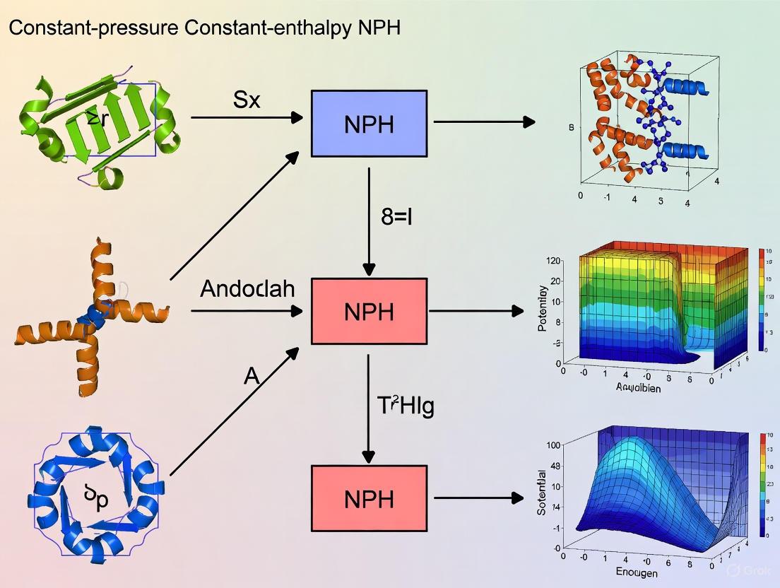
Performing a molecular dynamics (MD) simulation in the NPH ensemble requires specific algorithms to maintain constant pressure and conserve enthalpy. The following diagram illustrates the logical workflow and key parameter choices for configuring an NPH simulation.

Diagram 1: NPH Ensemble Simulation Workflow

A typical INCAR file configuration for an NPH run using the VASP software package, for instance, includes the key parameters shown in the workflow [8]:

• MDALGO = 3 to select the Langevin thermostat algorithm.
• ISIF = 3 to ensure the stress tensor is computed and the box volume and shape are allowed to change.
• LANGEVIN_GAMMA = 0.0 and LANGEVIN_GAMMA_L = 0.0 to disable the stochastic and friction terms of the Langevin thermostat and barostat, respectively. This leaves the box dynamics to be governed solely by the kinetic stress tensor, creating the conditions for an isoenthalpic ensemble.
• PMASS defines the mass of the barostat, controlling the inertia of the lattice degrees of freedom.

It is highly recommended to first equilibrate the system with an NPT molecular dynamics run to achieve the desired temperature and pressure before switching to the NPH ensemble for production data collection [8].

Application in Melting Point Calculations

The NPH ensemble has proven particularly valuable in methods for calculating melting temperatures (T_M) via molecular dynamics simulation. In the two-phase coexistence method, a system containing both solid and liquid phases is simulated. While this can be done in the NPT ensemble, it can lead to stress anisotropy (P_xx ≠ P_yy ≠ P_zz) due to interfacial stress. Performing the simulation in the NPH ensemble solves this problem because the three principal components of the stress tensor can be regulated to match the given pressure, leading to more accurate results [3].

Table 2: Comparison of Methods for Calculating Melting Temperature (T_M)

Method	Ensemble(s) Used	Key Principle	Reported Accuracy/Challenges
Two-Phase Coexistence	NPT, NVT, NPH	Direct simulation of solid-liquid equilibrium; TM is where both phases coexist.	High accuracy when stress anisotropy is handled (e.g., with NPH).
Hysteresis	NPT	Heating solid and cooling liquid; TM estimated empirically from hysteresis loop.	Low accuracy; strongly dependent on heating/cooling rate.
Interface Pinning	NPT	Uses an order parameter to pin the interface and measure chemical potential difference.	High accuracy, but ignores interface disorder.
Frenkel-Ladd (Thermodynamic Integration)	NVT	Calculates absolute Gibbs free energy for solid and liquid phases.	Very high accuracy, but computationally expensive and complex.
Void Method	NPT	Introduces a void to catalyze melting; TM is observed from property discontinuity.	Moderate accuracy; observational without firm thermodynamic principle.

Experimental Measurement of Binding Enthalpy

Isothermal Titration Calorimetry (ITC)

In pharmaceutical research, the binding enthalpy (ΔH) is not merely a theoretical concept but a measurable parameter with profound implications for drug candidate quality. The primary experimental technique for directly measuring the binding enthalpy is Isothermal Titration Calorimetry (ITC) [9]. ITC works by titrating a ligand solution into a protein solution and precisely measuring the heat released or absorbed upon binding. A single ITC experiment provides the binding constant (K_a), the stoichiometry (n), and the binding enthalpy (ΔH). The entropy change (ΔS) is then calculated using the relationship ΔG = ΔH - TΔS = -RT ln K_a [12] [13].

The Enthalpy Screen Protocol

To overcome the traditional low-throughput limitation of ITC, an "Enthalpy Screen" protocol has been developed. This method allows for the rapid determination of binding enthalpy for hundreds of ligands, making it suitable for the early stages of drug discovery following high-throughput screening [12].

The core principle involves injecting a small volume of a concentrated protein solution into a calorimetric cell containing the ligand at a concentration significantly exceeding its dissociation constant ([Ligand] >> K_d). This ensures that >99% of the injected protein binds to the ligand, and the measured heat effect is directly proportional to the binding enthalpy, requiring no complex fitting to a binding model [12]. The binding enthalpy is calculated using the equation:

ΔH = (Q_Inh - Q_Buf) / (V_Inj × [P])

where Q_Inh is the heat from injecting protease into the inhibitor solution, Q_Buf is the heat of dilution from injecting into buffer alone, V_Inj is the injection volume, and [P] is the concentration of active protein [12].

Table 3: Key Research Reagents and Materials for ITC and Enthalpy Screening

Reagent / Material	Specification / Function	Example from HIV-1 Protease Study [12]
Target Protein	Purified, active protein; concentration must be accurately determined.	HIV-1 protease (88% active concentration).
Ligands / Inhibitors	Compounds of interest dissolved in a compatible solvent.	KNI-series inhibitors (e.g., KNI-10769, KNI-577). Clinical inhibitors (e.g., amprenavir, indinavir).
Buffer System	Provides stable pH and ionic strength; must be free of contaminating reactants.	10 mM sodium acetate buffer, pH 5.0.
Solvent	Dissolves ligands; must be accounted for in control experiments.	DMSO (2% final concentration in experiments).
Calorimeter	Instrument for precise measurement of heat changes.	Affinity ITC (TA Instruments) with autosampler.
96-Well Plates	For high-throughput automated screening of multiple compounds.	Used by the autosampler for storing protein and ligand solutions.

Implications for Drug Discovery and Development

The thermodynamic signature of a drug candidate—the balance of enthalpic (ΔH) and entropic (-TΔS) contributions to binding—has emerged as a critical metric for assessing compound quality. Favorable binding enthalpy is associated with strong, specific interactions such as hydrogen bonds and van der Waals contacts that are geometrically optimal [12] [10]. Conversely, an unfavorable binding enthalpy often indicates that polar groups in the drug have been desolvated without forming productive new bonds with the target, a energetically costly process [12].

The evolution of two major drug classes, HIV-1 protease inhibitors and statins (cholesterol-lowering drugs), reveals a clear trend: later-generation "best in class" drugs consistently show more favorable binding enthalpies compared to the "first in class" pioneers [9] [10]. For example, the potent HIV-1 protease inhibitor darunavir has a markedly favorable binding enthalpy of -12.7 kcal/mol [10]. This improvement is not typically the primary goal of optimization efforts, which focus on potency, selectivity, and pharmacokinetics. However, it appears that achieving these goals often results in a molecule with a superior enthalpic profile, underscoring its importance as an indicator of overall compound quality.

A significant challenge in enthalpic optimization is the phenomenon of enthalpy-entropy compensation, where a gain in binding enthalpy is offset by a loss of binding entropy, resulting in little net improvement in affinity [9]. Overcoming this compensation is a primary objective in modern drug design. Strategies include ensuring that newly formed hydrogen bonds are geometrically optimal and that conformational flexibility is minimized before binding, reducing the entropic penalty upon complex formation [9] [10].

The thermodynamic identity H = E + PV and the principle of enthalpy conservation in the NPH ensemble provide a powerful framework for understanding and manipulating the behavior of systems at constant pressure. From computational material science, where the NPH ensemble enables accurate determination of properties like melting points, to experimental drug discovery, where the direct measurement of binding enthalpy guides the optimization of therapeutic compounds, the implications are vast and profound. The integration of thermodynamic principles, particularly through the use of enthalpy screens and structure-thermodynamic relationships, is paving the way for a new generation of highly optimized, "best in class" drugs. As molecular simulation tools and calorimetric techniques continue to advance, the explicit consideration of enthalpy and its interplay with entropy will undoubtedly become even more deeply embedded in the rational design of novel materials and pharmaceuticals.

In molecular dynamics (MD) simulations, the choice of statistical ensemble is foundational, determining the thermodynamic conditions and the fundamental properties of the system under study. An ensemble is a collection of system microstates that represent possible scenarios under a set of controlled macroscopic parameters [14]. Within a broader research context on the constant-pressure constant-enthalpy (NPH) ensemble, understanding its unique role and how it contrasts with the more common microcanonical (NVE), canonical (NVT), and isothermal-isobaric (NPT) ensembles is critical for advanced applications in materials science and drug development. These ensembles are artificial constructs that facilitate the calculation of macroscopic properties by holding different variables constant, thereby mimicking various experimental conditions [4] [14]. This guide provides a technical comparison of these ensembles, with a specific focus on elucidating the NPH ensemble's principles, implementation, and application.

Theoretical Foundations of Statistical Ensembles

Definition of Ensembles and Partition Functions

The mathematical description of an ensemble is encapsulated by its partition function, which contains all the thermodynamic information about the system [15]. The following table summarizes the core characteristics of the four ensembles examined in this overview.

Table 1: Fundamental Characteristics of Molecular Dynamics Ensembles

Ensemble	Name	Constant Parameters	Partition Function Relation	Conserved Quantity
NVE	Microcanonical	Number (N), Volume (V), Energy (E)	[15]	Total Energy (E)
NVT	Canonical	Number (N), Volume (V), Temperature (T)	[15]	Helmholtz Free Energy (F)
NPT	Isothermal-Isobaric	Number (N), Pressure (P), Temperature (T)	[15]	Gibbs Free Energy (G)
NPH	Isoenthalpic-Isobaric	Number (N), Pressure (P), Enthalpy (H)	[15]	Enthalpy (H = E + PV)

The NPH Ensemble: A Detailed Examination

The NPH ensemble is the analogue of the constant-volume, constant-energy (NVE) ensemble but under constant pressure conditions [4]. In this ensemble, the enthalpy (H), which is the sum of the internal energy (E) and the product of pressure and volume (PV), is conserved, barring numerical inaccuracies [8]. The partition function for the NpH ensemble is derived from the number of microstates consistent with a given enthalpy, H [15]. This ensemble visualizes a system of N particles in a box without rigid boundaries that is thermally isolated from its surroundings. The absence of rigid sides allows the volume and shape to change in response to pressure differences, causing the instantaneous pressure to fluctuate around the desired value [15].

Comparative Analysis of Ensemble Properties and Equations of Motion

Thermodynamic and Dynamic Control

The core difference between ensembles lies in which thermodynamic variables are controlled and which are allowed to fluctuate. These differences necessitate different algorithms and "extended system" methods to integrate the equations of motion while respecting the ensemble's constraints [16] [17].

Table 2: Operational Comparison of MD Ensembles

Ensemble	Fluctuating Quantities	Common Algorithms & Control Methods	Energy Conservation
NVE	Temperature, Pressure	Newton's Equations; Verlet/Velocity Verlet integrator [4] [18]	Yes (in theory) [14]
NVT	Energy, Pressure	Thermostats (e.g., Nosé-Hoover, Andersen, Berendsen) [14] [19]	No (dH/dt ≠ 0) [14]
NPT	Energy, Volume	Thermostat + Barostat (e.g., Parrinello-Rahman) [14] [16]	No
NPH	Temperature, Volume	Barostat only (e.g., in VASP: MDALGO=3 with zero Langevin constants) [8]	Yes (Enthalpy, H) [4]

Practical Implications of Fluctuations

The choice of ensemble directly impacts the physical significance of fluctuations in the simulation. For instance, in the NVE ensemble, the total energy is a constant of motion, but temperature fluctuates as the system explores regions of high and low potential energy on a fixed Potential Energy Surface (PES) [14]. In contrast, the NVT ensemble uses a thermostat to maintain a constant temperature, allowing the total energy to fluctuate. This means the system can effectively move from one PES to another, which is particularly useful for overcoming energy barriers [14]. The NPT ensemble introduces volume fluctuations on top of energy fluctuations, allowing the system's density to equilibrate at a given temperature and pressure. The NPH ensemble, conserving enthalpy, is characterized by fluctuations in temperature and volume, making it suitable for simulating adiabatic processes.

A Workflow for Ensemble Selection in Molecular Dynamics

The following diagram illustrates a logical decision-making process for selecting an appropriate ensemble based on the goals of a molecular dynamics simulation, positioning the NPH ensemble within the broader context of MD research.

Figure 1: MD Ensemble Selection Workflow. This diagram outlines the decision pathway for choosing the most appropriate statistical ensemble for a molecular dynamics simulation, based on the thermodynamic constraints of the system and the research objectives.

Detailed Experimental Protocol for NPH Ensemble Simulation

Prerequisites and Equilibration

Before initiating a production run in the NPH ensemble, it is strongly recommended to first equilibrate the system using an NPT molecular dynamics simulation. This ensures the system reaches the desired temperature and pressure, establishing a stable starting point for the subsequent NPH run [8].

Step-by-Step NPH Setup in VASP

The following protocol provides a detailed methodology for configuring an NPH ensemble simulation within the VASP software environment, a common tool in computational materials science [8].

Table 3: Research Reagent Solutions for NPH Ensemble Simulation in VASP

Item (INCAR Tag)	Function / Setting	Technical Specification
Molecular Dynamics Algorithm (MDALGO)	Selects the MD algorithm and thermostat.	Must be set to 3 to use the Langevin framework [8].
Langevin Barostat Friction (LANGEVINGAMMAL)	Controls the friction and stochastic term for the barostat.	Must be set to 0.0 to remove stochastic/friction terms, leaving box updates dependent on the kinetic stress tensor [8].
Langevin Thermostat Friction (LANGEVIN_GAMMA)	Controls the friction and stochastic term for the atomic thermostat.	Must be set to 0.0 for all atomic degrees of freedom to disable thermostatting, allowing velocities to be determined solely by interatomic forces [8].
Lattice Mass Parameter (PMASS)	Controls the inertia of the lattice degrees of freedom.	Must be set to a value > 0.0; specific value depends on the system and desired dynamics [8].
Integration Time Step (POTIM)	Defines the time step for numerical integration.	Typically 1.0 fs for systems with atoms, but can be system-dependent [19].
Stress Tensor Control (ISIF)	Determines whether volume/shape is fixed or allowed to change.	Set to 3 to compute the stress tensor and allow changes in box volume and shape [8] [19].

Procedure:

• Initial Configuration: Prepare a POSCAR file containing the atomic positions of a sufficiently large supercell [19].
• INCAR Parameterization: In the main input file (INCAR), set the following critical tags as specified in Table 3 [8]:
  • IBRION = 0 (to enable MD)
  • MDALGO = 3
  • ISIF = 3
  • LANGEVIN_GAMMA_L = 0.0
  • LANGEVIN_GAMMA = 0.0
  • PMASS = [value] (user-defined)
  • POTIM = [value] (e.g., 1.0)
  • NSW = [number_of_steps]
• Execution: Compile VASP with the -Dtbdyn preprocessor flag and execute the program [19].
• Validation: Monitor the output (e.g., in OUTCAR or OSZICAR) to confirm that the enthalpy (H) is conserved throughout the simulation and that the pressure fluctuates around the target equilibrium value.

Applications and Best Practices

Recommended Use Cases for Each Ensemble

• NVE Ensemble: Primarily used for studying fundamental dynamic properties and energy conservation, or for exploring a system's Potential Energy Surface (PES) [4] [14]. It is not recommended for equilibration as it cannot drive the system to a desired temperature [4].
• NVT Ensemble: The default choice for many simulations, especially when conformational searches are performed in vacuum or without periodic boundary conditions [4]. It is ideal when the system volume and lattice vectors must be held constant, such as in simulations of solids or when measuring pressure at system boundaries is a concern [14].
• NPT Ensemble: The ensemble of choice when correct pressure, volume, and density are critical, as it best mimics standard experimental conditions [4]. It is essential for studying phase transitions, self-assembly processes (e.g., bilayer formation), and for achieving equilibrium density [14] [20].
• NPH Ensemble: As an analogue to NVE under constant pressure, it is useful for simulating adiabatic processes where no heat exchange occurs. It is also employed as a test for numerical stability and to check if a system is sufficiently equilibrated before starting production runs [20].

Critical Considerations for Practitioners

• Ergodicity and Sampling: All ensembles should, in principle, produce consistent averages for the same state point, but their fluctuations differ [4]. Inadequate sampling can violate ergodicity, leading to incorrect time-averaged properties [14].
• Physical Meaning without PBCs: Without Periodic Boundary Conditions (PBCs), volume, pressure, and density are not well-defined. Therefore, constant-pressure dynamics (NPT, NPH) cannot be performed, and NVT is the appropriate choice [4] [20].
• Numerical Stability: Energy drift in NVE due to integration errors is common [4]. Running a system in NVE after equilibration is often used as a stability test for the simulation parameters and potentials [20].

The study of thermodynamic ensembles provides the foundation for understanding and predicting the behavior of molecular systems. The isoenthalpic–isobaric (NPH) ensemble, where particle number (N), pressure (P), and enthalpy (H) remain constant, represents a specific set of natural conditions crucial for simulating various physical processes. Enthalpy (H) is defined as the sum of a thermodynamic system's internal energy (U) and the product of its pressure and volume (pV), expressed as H = U + pV [21]. This state function becomes particularly valuable when examining systems at constant external pressure, a condition conveniently provided by Earth's ambient atmosphere in experimental settings [21].

Understanding when a system naturally maintains constant enthalpy is fundamental to multiple scientific domains, including drug development, where accurate simulation of biomolecular interactions under specific thermodynamic conditions can predict binding affinities and stability. The NPH ensemble serves as the constant-pressure analogue to the constant-volume, constant-energy (NVE) ensemble, making it indispensable for studying processes where energy exchange occurs through work rather than heat transfer [4]. This technical guide explores the theoretical foundations, practical implementations, and research applications of isoenthalpic systems within the broader context of constant-pressure, constant-enthalpy ensemble research.

Theoretical Foundations of Constant Enthalpy

The Isoenthalpic–Isobaric (NPH) Ensemble

The isoenthalpic–isobaric ensemble maintains constant enthalpy (H) and constant pressure (P) while allowing volume (V) to fluctuate [1]. In this ensemble, the system can exchange energy with its environment through work (pV work) but not through heat transfer, creating an adiabatic system at constant pressure. The conservation of enthalpy in this ensemble arises directly from its definition: H = E + PV, where E represents the internal energy [1].

In statistical mechanics, the NPH ensemble provides a framework for calculating thermodynamic averages when pressure rather than volume is the controlled variable. This proves particularly useful for comparing simulation results with experimental measurements, which are often conducted under constant pressure conditions [4]. The connection between molecular dynamics and the NPH ensemble emerges from the equations of motion, which can be formulated to conserve enthalpy while allowing the simulation box volume to adjust in response to pressure differences.

Natural Conditions for Constant Enthalpy

A system naturally maintains constant enthalpy under specific physical conditions, primarily characterized by the absence of heat exchange with the environment while pressure remains constant. These adiabatic, isobaric processes occur when:

• Perfect Thermal Insulation: The system is completely isolated from heat transfer with its surroundings (adiabatic condition) [22].
• Constant External Pressure: The system experiences a fixed external pressure, typically from the environment [21].
• No Non-pV Work: The system does not perform or receive work other than pressure-volume work [22].

Under these conditions, any change in the system's internal energy (ΔU) must equal the negative of the pV work done (-PΔV), leading to zero change in enthalpy (ΔH = ΔU + PΔV = 0) [21]. In molecular dynamics simulations, these conditions are engineered through specific algorithms that control pressure without implementing a thermostat, allowing the temperature to fluctuate freely while conserving enthalpy [8].

Table 1: Characteristic Conditions for Constant Enthalpy in Different System Types

System Type	Adiabatic Condition	Pressure Condition	Resulting Enthalpy Behavior
Isolated Physical System	Perfect thermal insulation	Constant external pressure	Naturally constant enthalpy
NPH Molecular Dynamics	No thermostat applied	Barostat maintains constant pressure	Enthalpy conserved (within numerical precision)
Chemical Reaction	No heat exchange with surroundings	Open to atmosphere	Enthalpy change approximately zero

NPH Ensemble in Molecular Dynamics Simulations

Implementation and Equations of Motion

In molecular dynamics simulations, the NPH ensemble is implemented through specialized integrators that modify the equations of motion to maintain constant pressure while conserving enthalpy. The equations of motion for NPH dynamics are given by [23]:

Where:

• ri and pi are atom i's position and momentum, respectively
• mi is the mass of atom i
• fi is the force on atom i
• V is the system volume
• W is the piston mass parameter
• P(t) is the instantaneous pressure
• Pext is the external pressure
• γ is the collision frequency
• R(t) is a random force (zero when implementing pure NPH)

These equations describe a system where the volume adjusts dynamically in response to pressure differences through a "piston" with mass W, while no thermal coupling exists to maintain constant temperature [23]. The absence of a thermostat results in temperature fluctuations that maintain constant enthalpy as the volume changes.

Table 2: Key Parameters in NPH Molecular Dynamics Implementation

Parameter	Symbol	Role in NPH Dynamics	Typical Units
Piston Mass	W	Controls inertia of volume fluctuations; affects stability and oscillation frequency	amu (atomic mass units)
External Pressure	Pext	Target pressure value maintained by barostat	bar, atm, MPa
Instantaneous Pressure	P(t)	Current internal pressure of system, calculated from virial	bar, atm, MPa
Collision Frequency	γ	Damping coefficient for piston motion (zero in pure NPH)	ps-1
Time Step	Δt	Integration interval for equations of motion	fs (femtoseconds)

Practical Simulation Protocols

Implementing NPH ensemble simulations requires specific configuration of molecular dynamics packages. For example, in VASP, an NPH simulation is configured as follows [8]:

• Ensemble Selection: Set MDALGO = 3 to use the Langevin thermostat algorithm
• Thermostat Disabling: Set LANGEVIN_GAMMA = 0.0 and LANGEVIN_GAMMA_L = 0.0 to remove stochastic and friction terms
• Barostat Configuration: Set ISIF = 3 to compute stress tensor and allow volume changes
• Piston Mass: Adjust PMASS to control the inertia of lattice degrees of freedom

Similar implementations exist in other molecular dynamics engines. For instance, apoCHARMM supports NPH dynamics using a Langevin piston barostat with the random force term disabled [23]. CASTEP includes NPH as one of its core thermodynamic ensembles, particularly useful for studying materials under pressure [24].

A critical prerequisite for successful NPH simulations is proper system equilibration. It is recommended to first equilibrate the system using an NPT (constant temperature and pressure) ensemble to achieve the desired temperature and pressure before switching to NPH production runs [8]. This ensures the system starts from appropriate initial conditions while maintaining constant enthalpy throughout the data collection phase.

Research Applications and Experimental Considerations

Phase Transition Studies

The NPH ensemble proves particularly valuable for studying phase transitions in materials, as it naturally captures the enthalpy changes associated with these transformations. In one documented approach, researchers simulate supercooled liquids and detect phase transitions by slowly reducing enthalpy in a series of NPH runs, artificially extracting kinetic energy through velocity rescaling between simulations [25]. This method enables direct observation of latent heat release during phase transitions, as at constant pressure, changes in enthalpy equal the heat that enters or leaves the system [25].

This application highlights a key advantage of the NPH ensemble: the direct correspondence between enthalpy changes and heat transfer at constant pressure makes it ideal for quantifying thermodynamic properties associated with phase transformations. The ability to control enthalpy rather than temperature provides a more natural framework for studying these processes, particularly when comparing simulation results with experimental calorimetry data.

Comparison with Other Thermodynamic Ensembles

The NPH ensemble occupies a specific niche within the spectrum of thermodynamic ensembles used in molecular simulations. Understanding its relationship to other ensembles helps researchers select the appropriate method for their specific research questions.

Table 3: Comparison of Major Molecular Dynamics Ensembles

Ensemble	Fixed Quantities	Fluctuating Quantities	Primary Research Applications
NVE	Number of particles, Volume, Energy	Temperature, Pressure	Energy-conserving dynamics; fundamental studies [4]
NVT	Number of particles, Volume, Temperature	Energy, Pressure	Conformational sampling; biomolecular folding [4]
NPT	Number of particles, Pressure, Temperature	Energy, Volume	Standard conditions matching experiments; equilibration [4]
NPH	Number of particles, Pressure, Enthalpy	Energy, Temperature, Volume	Phase transitions; adiabatic processes [4] [24]

The following diagram illustrates the decision process for selecting an appropriate ensemble based on the natural conditions of the system being studied:

Systematic selection of thermodynamic ensembles for molecular simulations

Implementing NPH ensemble research requires both specific computational tools and theoretical frameworks. The following table details key resources essential for conducting isoenthalpic-isobaric simulations.

Table 4: Essential Research Resources for NPH Ensemble Simulations

Resource Category	Specific Tool/Method	Function in NPH Research
Molecular Dynamics Software	VASP [8], apoCHARMM [23], CASTEP [24]	Implements NPH equations of motion; provides barostat algorithms
Barostat Algorithms	Langevin Piston [23], Parrinello-Rahman [24]	Maintains constant pressure by adjusting simulation box volume
Analysis Methods	Enthalpy Calculation [21], Virial Computation [23]	Monitors enthalpy conservation; calculates pressure from atomic forces
Theoretical Frameworks	Isoenthalpic–isobaric Ensemble Theory [1]	Provides statistical mechanical basis for interpreting results
System Preparation	NPT Equilibration Protocol [8]	Achieves target temperature/pressure before NPH production runs

The theoretical basis for when a system naturally maintains constant enthalpy is firmly rooted in the conditions of the isoenthalpic–isobaric ensemble: adiabatic boundaries that prevent heat transfer, constant external pressure, and the absence of non-pV work. These conditions create an environment where enthalpy remains constant despite internal energy and volume fluctuations. The NPH ensemble provides both a theoretical framework and practical methodology for studying such systems through molecular dynamics simulations.

For researchers in drug development and materials science, understanding and utilizing the NPH ensemble offers unique insights into processes where enthalpy, rather than temperature, serves as the controlling thermodynamic variable. Phase transition studies, materials under pressure, and processes mimicking adiabatic conditions in real-world applications all benefit from the isoenthalpic perspective. As molecular dynamics software continues to advance, with packages like apoCHARMM providing enhanced virial calculations and more efficient NPH implementations [23], the research applications of constant-enthalpy simulations will continue to expand, offering new opportunities for connecting simulation data with experimental observations under naturally occurring isoenthalpic conditions.

Fundamental Properties and Fluctuations Accessible in the NPH Ensemble

The isoenthalpic-isobaric (NPH) ensemble represents a fundamental statistical mechanical framework for studying materials under constant particle number (N), pressure (P), and enthalpy (H). Unlike the more commonly employed NPT ensemble that maintains constant temperature, the NPH ensemble provides direct access to adiabatic processes and thermodynamic properties derivable from enthalpy conservation. This technical guide explores the core theoretical foundations, practical implementation methodologies, and key applications of NPH ensemble simulations, with particular emphasis on the analysis of fluctuations and their relationship to material properties. Designed for computational researchers and drug development professionals, this work establishes the NPH ensemble's unique capabilities for investigating pressure-induced phase transitions, nanomaterial behavior, and biological systems under physiologically relevant conditions.

Theoretical Foundations of the NPH Ensemble

The NPH ensemble is characterized by fixed particle number (N), pressure (P), and enthalpy (H), making it the constant-pressure analogue to the microcanonical (NVE) ensemble [4]. The fundamental thermodynamic potential conserved in this ensemble is enthalpy, defined as H = E + PV, where E represents the internal energy and PV denotes the pressure-volume work term [1]. This conservation relationship dictates that fluctuations in internal energy are directly coupled to fluctuations in the system volume through the constant pressure constraint.

In molecular dynamics simulations, the NPH ensemble enables the study of systems where energy exchange occurs through mechanical work rather than heat transfer with a thermal reservoir. The statistical sampling in the NPH ensemble provides direct access to the isothermal compressibility (κₜ) through volume fluctuations according to the relation [4]:

[ \langle (\Delta V)^2 \rangle = kB T V \kappaT ]

where ⟨(ΔV)²⟩ represents the mean-squared volume fluctuations, k_B is Boltzmann's constant, T is temperature, V is volume, and κₜ is the isothermal compressibility. This relationship demonstrates how measurable fluctuations in simulation observables connect to fundamental thermodynamic response functions.

The NPH ensemble is particularly valuable for investigating adiabatic processes where no heat exchange occurs, making it ideally suited for modeling rapid compression/expansion phenomena, shock waves, and other processes where thermal equilibration with the environment is significantly slower than the timescale of mechanical work transfer. For drug development applications, this corresponds to physiological processes involving rapid pressure changes or mechanical stress on biological macromolecules.

Practical Implementation in Molecular Dynamics

Simulation Methodology

Implementing the NPH ensemble in molecular dynamics requires specific algorithmic approaches and parameter configurations. In the VASP software package, the NPH ensemble is activated by setting MDALGO = 3 while disabling thermostatting through appropriate parameter selection [8]. The key implementation steps include:

Equation of Motion Integration: The NPH ensemble utilizes extended Lagrangian formulations that incorporate barostat degrees of freedom to maintain constant pressure. The lattice vectors fluctuate in response to the difference between the internal and external pressure, with the inertia of these fluctuations controlled by the PMASS parameter [8].

Barostat Configuration: Proper selection of the barostat mass parameter (PMASS) is critical for achieving efficient sampling without introducing artificial oscillatory behavior in volume fluctuations. The recommended practice involves system equilibration using the NPT ensemble before transitioning to NPH production runs [8].

Numerical Stability Considerations: The absence of thermostating in NPH simulations necessitates careful monitoring of numerical drift. Using time-reversible integrators and sufficiently small timesteps (typically 1-2 femtoseconds for atomistic systems) ensures acceptable energy conservation within the discrete integration scheme [8].

Table 1: Key Parameters for NPH Ensemble Implementation in VASP

Parameter	Required Value	Function	Considerations
MDALGO	3	Selects Langevin dynamics algorithm	Must be combined with appropriate ISIF setting
ISIF	3	Enables stress tensor calculation and volume/shape changes	Essential for pressure control
LANGEVIN_GAMMA	0.0	Disables thermostat friction term	Creates isoenthalpic conditions
LANGEVINGAMMAL	0.0	Disables barostat stochastic term	Maintains constant enthalpy
PMASS	Variable	Sets inertia of lattice degrees of freedom	System-dependent optimization required

Simulation Workflow

The following diagram illustrates the complete workflow for setting up and running an NPH ensemble simulation, from system preparation through to data analysis:

Sample Input Configuration

A representative INCAR file for NPH ensemble simulations in VASP demonstrates the critical parameter combinations [8]:

This configuration maintains constant enthalpy by eliminating stochastic and frictional terms from both thermostats and barostats, allowing the system to evolve according to the deterministic equations of motion under constant pressure conditions.

Key Properties and Fluctuation Analysis

Accessible Thermodynamic Properties

The NPH ensemble provides direct measurement capabilities for several important thermodynamic response functions through the analysis of trajectory fluctuations. The conserved enthalpy constraint creates specific relationships between energy and volume fluctuations that can be exploited to extract material properties.

Table 2: Thermodynamic Properties Accessible from NPH Ensemble Fluctuations

Property	Fluctuation Relation	Physical Significance	Application Context
Isothermal Compressibility (κₜ)	⟨(ΔV)²⟩ = kBT V κₜ	Resistance to uniform compression	Hydration behavior in drug binding
Thermal Expansion Coefficient (α)	⟨ΔV ΔH⟩ = kBT² V α / κₜ	Volume change with temperature at constant pressure	Polymer swelling in physiological conditions
Constant-Pressure Heat Capacity (Cₚ)	⟨(ΔH)²⟩ = kBT² Cₚ	Energy required to raise temperature at constant pressure	Protein stability under pressure stress
Adiabatic Compressibility (κₛ)	κₛ = κₜ - TVα²/Cₚ	Compression at constant entropy	Sound propagation in biomaterials

Successful implementation of NPH ensemble simulations requires both specialized software tools and carefully parameterized force fields. The following table details essential components of the computational researcher's toolkit for NPH investigations:

Table 3: Research Reagent Solutions for NPH Ensemble Simulations

Tool/Resource	Function	Application Notes
VASP	First-principles molecular dynamics with NPH capability	Implements NPH via MDALGO=3; suitable for periodic systems [8]
LAMMPS	Classical molecular dynamics with extended Lagrangian methods	Supports NPH using fix nph command; extensive force field compatibility
AMBER	Biomolecular simulation package	Specialized for pharmaceutical applications; constant-pressure methods
CHARMM	All-atom empirical force field	Optimized for proteins, nucleic acids, and lipids in NPH contexts
GAUSSIAN	Electronic structure calculations	Provides quantum mechanical reference data for force field parameterization
PLUMED	Enhanced sampling and analysis	Facilitates calculation of fluctuation-based thermodynamic properties

Applications in Drug Development and Materials Research

The NPH ensemble offers unique advantages for pharmaceutical applications where pressure fluctuations occur naturally or represent an important experimental variable. In drug delivery systems, the behavior of lipid bilayers, polymeric nanoparticles, and protein therapeutics under pressure stress can be directly simulated using NPH methodologies.

For encapsulated drug formulations, the NPH ensemble enables prediction of stability under various pressure conditions encountered during manufacturing, storage, and administration. The volume fluctuations accessible through NPH simulations correlate directly with packing efficiency and void distribution in amorphous solid dispersions—critical factors influencing drug recrystallization and release kinetics.

Additionally, pressure-induced denaturation of biopharmaceuticals represents an important degradation pathway that can be systematically investigated using NPH approaches. The ensemble's ability to model adiabatic compression events provides molecular-level insights into protein unfolding transitions under high-pressure processing conditions used for sterilization of therapeutic proteins.

The fluctuation properties derived from NPH simulations further enable prediction of thermodynamic stability boundaries for polymorphic drug crystals, supporting the design of robust crystalline forms with optimal bioavailability and processing characteristics.

The NPH ensemble constitutes a powerful framework for investigating thermodynamic properties and material behavior under constant-pressure, constant-enthalpy conditions. Through careful implementation and fluctuation analysis, researchers can access fundamental response functions including compressibility, thermal expansion, and heat capacity—properties essential for rational design in pharmaceutical development and advanced materials engineering. The continued refinement of NPH simulation methodologies promises enhanced predictive capabilities for systems subject to mechanical stress and pressure perturbations, bridging molecular-scale interactions with macroscopic material performance.

Implementing NPH Simulations: Setup, Workflow, and Real-World Applications

Step-by-Step Guide to Configuring an NPH Simulation in VASP (MDALGO=3)

The isoenthalpic-isobaric (NpH) ensemble is a fundamental tool in molecular dynamics (MD) simulations for studying materials under constant pressure and enthalpy conditions. This ensemble is particularly valuable for investigating systems where energy exchange is restricted, mimicking adiabatic processes common in high-pressure physics, materials science, and drug development research. Within the Vienna Ab initio Simulation Package (VASP), the NpH ensemble is implemented through specific MD algorithms and parameter configurations. This technical guide provides researchers with a comprehensive framework for configuring, executing, and validating NpH simulations in VASP using the MDALGO = 3 parameter, enabling accurate modeling of materials behavior under controlled thermodynamic conditions.

Theoretical Foundations of the NpH Ensemble

Ensemble Theory and Thermodynamic Relationships

In statistical mechanics, the NpH ensemble represents a collection of systems with constant particle number (N), constant pressure (p), and constant enthalpy (H). The isoenthalpic-isobaric partition function is mathematically defined as: [ X(N,p,H) = \sum{H-\delta H{i}},{\mathbf{p}_{i}}) ] where the summation includes all microstates compatible with the enthalpy constraints [15]. Each microstate in this ensemble occurs with equal probability, making it the appropriate statistical mechanical foundation for modeling adiabatic processes at constant external pressure.+\delta>(n,p,{\mathbf{r}

The NpH ensemble can be visualized as an N-particle system in a box without rigid boundaries that is thermally isolated from its surroundings. Since the box has no fixed sides, the volume and shape fluctuate according to the pressure difference between the interior and exterior of the simulation cell. In practical simulations, the instantaneous pressure fluctuates around the target value, while the enthalpy remains conserved within numerical precision [15]. This makes the NpH ensemble particularly suitable for modeling processes in materials science and pharmaceutical development where systems experience pressure changes without heat exchange with the environment.

Comparison with Other Ensembles

The NpH ensemble occupies a distinct position in the landscape of statistical ensembles commonly used in molecular dynamics simulations:

• Microcanonical (NVE) ensemble: Characterized by constant particle number (N), volume (V), and energy (E), this ensemble completely isolates the system from its environment. Unlike NpH, it maintains fixed volume rather than fixed pressure.

• Canonical (NVT) ensemble: Maintains constant particle number (N), volume (V), and temperature (T) through thermal contact with a heat bath. While NVT allows energy exchange, NpH allows volume changes while conserving enthalpy.

• Isothermal-isobaric (NpT) ensemble: Keeps constant particle number (N), pressure (p), and temperature (T) through contact with both a heat bath and volume reservoir. The key distinction from NpH is that NpT allows energy exchange to maintain temperature, while NpH conserves enthalpy through thermal isolation [15].

The relationship between these ensembles becomes particularly important when designing multi-stage simulation protocols, where equilibration in one ensemble precedes production sampling in another.

Configuration Methodology for NpH Simulations

Core Parameter Specification

Implementing an NpH ensemble simulation in VASP requires precise configuration of key parameters in the INCAR file. These parameters control the molecular dynamics algorithm, thermostat behavior, and barostat settings to achieve the correct thermodynamic conditions.

Table 1: Essential INCAR Parameters for NpH Ensemble Simulations

Parameter	Required Value	Physical Significance	Technical Function
MDALGO	3	Selects Langevin dynamics	Enables the appropriate equations of motion for sampling the NpH ensemble
ISIF	3	Controls stress tensor handling	Computes stress tensor and allows changes to box volume and shape
LANGEVIN_GAMMA	0.0 for all species	Friction coefficient for atomic degrees of freedom	Disables thermostatting by removing friction and stochastic forces
LANGEVIN_GAMMA_L	0.0	Friction coefficient for lattice degrees of freedom	Disables barostat damping, leaving box evolution determined by kinetic stress
PMASS	User-defined (e.g., 10)	Fictitious mass for lattice degrees of freedom	Controls the inertia and dynamics of cell shape/volume fluctuations
PSTRESS	Optional	External pressure target	Sets the desired external pressure in kB

The MDALGO = 3 parameter activates the Langevin thermostat framework, which can sample various ensembles depending on additional parameter settings [26]. For NpH simulations, the critical distinction lies in completely disabling the stochastic and friction terms through zero values for both LANGEVIN_GAMMA and LANGEVIN_GAMMA_L. This ensures that the system evolves according to Newton's equations modified only by the barostat for pressure control, without thermal coupling that would alter the enthalpy [27].

The PMASS parameter deserves special attention as it controls the timescale of cell fluctuations. Heavier masses result in slower cell oscillations, while lighter masses may introduce artificial dynamics. Empirical testing is recommended to determine optimal values for specific systems, with typical values ranging from 5-20 atomic mass units for most materials.

Complete INCAR Template for NpH Simulations

Below is a comprehensive INCAR template configured for NpH ensemble simulations, incorporating both the essential dynamics parameters and recommended electronic structure settings:

This template represents a minimal configuration for NpH simulations. The electronic structure parameters (PREC, ENCUT, etc.) should be optimized for the specific system under investigation, while the core MD parameters remain consistent for NpH sampling [27].

Workflow Implementation and Experimental Protocol

Pre-equilibration Procedures

Proper equilibration is critical for obtaining physically meaningful results from NpH simulations. We recommend a multi-stage equilibration protocol:

• Initial Geometry Optimization: Begin with a conjugate gradient relaxation (IBRION = 2) of the initial structure to eliminate high-energy configurations and ensure a reasonable starting geometry.

• NVT Equilibration: Perform canonical ensemble equilibration using either Nosé-Hoover (MDALGO = 2) or Langevin dynamics (MDALGO = 3 with LANGEVIN_GAMMA > 0) to thermalize the system at the target temperature. Typical simulation lengths should encompass at least 5-10 ps for most systems.

• NpT Equilibration: Transition to isothermal-isobaric ensemble simulations (MDALGO = 3 with appropriate LANGEVIN_GAMMA and LANGEVIN_GAMMA_L values) to equilibrate the density at the target pressure and temperature. This stage allows the system to reach the appropriate volume for the specified thermodynamic conditions.

• NpH Production: Finally, initiate the NpH production simulation using the parameter specifications outlined in Section 2.1, using the final configuration from the NpT equilibration as the starting point [27].

This sequential equilibration approach ensures that the system reaches proper thermodynamic equilibrium before beginning production sampling in the NpH ensemble, minimizing transient effects and improving the statistical quality of the results.

Workflow Visualization

The following diagram illustrates the complete workflow for NpH simulations, from initial setup to production and analysis:

NpH Simulation Workflow

Research Reagent Solutions: Computational Materials

Essential Software Components

Successful NpH simulations require careful preparation of computational "reagents" - the input files and parameters that define the simulation. These components function analogously to laboratory reagents in experimental research:

Table 2: Essential Computational Materials for NpH Simulations

Component	Format	Function	Preparation Guidelines
INCAR	Text file	Controls simulation parameters	Must contain specific NpH tags: MDALGO=3, ISIF=3, LANGEVIN_GAMMA=0, LANGEVIN_GAMMA_L=0
POSCAR	Crystallographic	Defines initial atomic positions	Should originate from equilibrated NpT simulation; supercell size must accommodate long-wavelength vibrations
POTCAR	Pseudopotential	Describes electron-ion interactions	Must match atomic species in POSCAR; consistent functional (PAW-PBE recommended)
KPOINTS	Reciprocal space	Specifies k-point sampling	Should provide sufficient Brillouin zone sampling; Gamma-point may suffice for large supercells

The POSCAR file deserves particular attention in NpH simulations. Since the ensemble allows volume fluctuations, the initial structure should represent a reasonable starting density for the target pressure. Using a structure from a pre-equilibrated NpT simulation at the same pressure is strongly recommended. For complex molecular systems, such as those relevant to drug development, special care must be taken to ensure the simulation cell is large enough to minimize periodic image interactions [28].

Advanced Configuration: Machine Learning Force Fields

For systems requiring extended sampling beyond the capabilities of direct ab initio MD, machine learning force fields (MLFF) can be integrated with NpH simulations to dramatically enhance computational efficiency. The MLFF implementation in VASP enables on-the-fly learning of interatomic potentials during an initial ab initio MD simulation, which can then be deployed for extended sampling [29].

Key MLFF parameters for NpH simulations include:

• ML_LMLFF = .TRUE. activates the machine learning force field capability
• ML_ISTART = 0 initiates training of a new force field
• ML_CTIFOR sets the threshold for adding new configurations to the training set based on Bayesian error estimates

When combining MLFF with NpH simulations, the force field training occurs during the initial equilibration stages, with the production NpH simulation potentially using the trained force field for enhanced sampling. This approach can extend accessible timescales by 2-3 orders of magnitude while maintaining ab initio accuracy [29] [30].

Validation and Analysis Protocols

Ensemble Validation Metrics

Verifying proper sampling of the NpH ensemble requires monitoring specific thermodynamic quantities throughout the simulation:

• Enthalpy Conservation: The total enthalpy ( H = U + pV ) should remain constant throughout the simulation, with fluctuations attributable only to numerical integration error. Significant drift indicates improper isolation or parameter issues.

• Pressure Fluctuations: The instantaneous pressure should fluctuate around the target value (PSTRESS), with the average matching the external pressure setting.

• Drift Monitoring: The cumulative energy drift should be monitored to detect numerical instabilities or inadequate integration parameters.

The following diagram illustrates the key validation relationships and monitoring targets:

NpH Validation Metrics

Troubleshooting Common Issues

Even with proper configuration, NpH simulations may encounter numerical issues that require intervention:

• Energy Drift: Significant enthalpy drift may indicate that POTIM is too large. Reduce the timestep by 25-50% and test for improved conservation.

• Cell Oscillations: Excessive oscillation of cell parameters suggests that PMASS is too small. Increasing this parameter by a factor of 2-5 typically dampens artificial dynamics.

• Pressure Deviation: Consistent deviation from the target pressure may require adjustment of the PSTRESS value or verification of the stress tensor calculation through convergence testing of ENCUT and k-point sampling.

For systems with significant atomic mass disparities, the LANGEVIN_GAMMA parameters may need species-specific tuning, though they remain zero for strict NpH sampling. In such cases, minimal values that stabilize the dynamics without significant thermal coupling may be employed.

Applications in Research and Development

The NpH ensemble enables investigation of diverse phenomena across multiple disciplines. In pharmaceutical research, it facilitates study of drug molecule behavior under pressure conditions mimicking various administration routes or manufacturing processes. For materials science, NpH simulations provide insights into phase transitions, mechanical properties, and material responses to extreme pressure conditions.

Recent advances in specialized hardware, such as Molecular Dynamics Processing Units (MDPUs), promise to accelerate NpH simulations by up to 10³ times compared to conventional CPU/GPU implementations while maintaining ab initio accuracy [30]. These developments will make previously intractable problems accessible to molecular simulation, particularly in drug development where complex molecular systems require extensive sampling.

When properly configured and validated, NpH simulations in VASP provide a powerful tool for investigating pressure-induced phenomena across scientific disciplines, from fundamental materials physics to applied pharmaceutical research. The rigorous approach outlined in this guide ensures researchers can implement this technique with confidence in its thermodynamic foundation and numerical stability.

The NpH ensemble, or constant-pressure constant-enthalpy ensemble, provides a critical framework for studying materials and molecular systems under experimentally relevant conditions where pressure fluctuates around an equilibrium value while enthalpy is conserved. This technical guide details the strategic selection of three core parameters—PMASS, LANGEVIN_GAMMA, and ISIF—within the Vienna Ab initio Simulation Package (VASP) to correctly configure and execute reliable NpH simulations. Aimed at researchers and scientists in computational drug development and materials science, this whitepaper synthesizes current best practices, quantitative parameter recommendations, and experimental protocols to ensure accurate sampling of the isoenthalpic-isobaric ensemble for predictive molecular design.

In molecular dynamics (MD), the statistical ensemble defines the thermodynamic conditions under which a simulation proceeds. The NpH ensemble is characterized by a constant number of particles (N), a pressure that fluctuates around a fixed equilibrium value (p), and a conserved enthalpy (H) [8]. This makes it exceptionally valuable for simulating processes where the system exchanges energy with its environment as work, rather than heat, such as in the study of structural phase transitions, material response to mechanical stress, or biomolecular conformations in different pressure environments.

Within VASP, the NpH ensemble is activated by setting MDALGO = 3 (Langevin dynamics) and disabling thermostatting by setting both LANGEVIN_GAMMA = 0 and LANGEVIN_GAMMA_L = 0 [8]. This configuration ensures that the velocity of atoms is governed solely by the Hellmann-Feynman forces, and the box dynamics (barostatting) is driven exclusively by the kinetic stress tensor, without stochastic or frictional interference. The successful sampling of this ensemble hinges on the precise configuration of three interdependent parameters: PMASS (barostat mass), LANGEVIN_GAMMA (atomic friction), and ISIF (degree of cell freedom). Their careful selection is not merely a technical detail but a fundamental prerequisite for generating physically meaningful results that can underpin a broader thesis on constant-enthalpy research.

Theoretical Foundation and Parameter Definitions

The Langevin Equation in Extended System Dynamics

The implementation of the barostat in VASP's NpH ensemble is based on the Parrinello-Rahman method, extended for stochastic dynamics [8] [26]. The core equation of motion for the atoms incorporates the barostat coupling and, in its general form for the NpT ensemble, includes a Langevin thermostat. For the NpH ensemble, however, the thermostat terms are disabled. The simplified equation governing the lattice vectors can be conceptualized as: ML * Ä = (Pinternal - Pexternal) * V - γL * M_L * Ȧ Here, M_L is the inertia of the lattice degrees of freedom, controlled by PMASS, Ä and Ȧ are the second and first derivatives of the lattice vectors, P_internal and P_external are the internal and external pressures, V is the cell volume, and γ_L is the friction coefficient for the lattice, set to zero via LANGEVIN_GAMMA_L = 0 in NpH [8]. This equation describes a driven, damped oscillation of the cell shape and size around the equilibrium defined by the external pressure.

Core Parameter Definitions

• PMASS: Also known as the "fictitious mass" of the barostat, PMASS (in amu) determines the inertia of the lattice degrees of freedom. A higher PMASS leads to slower, more sluggish cell oscillations, while a lower value makes the cell respond more quickly to pressure differences.
• LANGEVIN_GAMMA: This parameter (in ps⁻¹) specifies the friction coefficient for the atomic degrees of freedom when using a Langevin thermostat [26] [31]. In the NpH ensemble, this is set to zero for all species, effectively turning off temperature control and allowing the system to evolve under adiabatic conditions [8].
• ISIF: This tag controls which degrees of freedom of the simulation cell are allowed to change and whether the stress tensor is calculated [8] [26]. For a fully flexible cell in the NpH ensemble, ISIF=3 must be used, which computes the stress tensor and allows changes to the cell's volume, shape, and ions' positions [8].

Quantitative Parameter Tables and Selection Guidelines

The selection of parameters is a balance between numerical stability, sampling efficiency, and physical accuracy. The following tables consolidate recommended values and their implications.

Table 1: Core INCAR Tags and Values for NpH Ensemble Simulations in VASP

INCAR Tag	Required Value for NpH	Function	Critical Interaction
MDALGO	3	Selects Langevin dynamics algorithm [8].	Must be combined with ISIF=3.
ISIF	3	Calculates stress tensor and allows changes to cell volume and shape [8].	Enables barostat action.
LANGEVIN_GAMMA	0.0 (for all species)	Disables atomic thermostatting [8].	Essential for isoenthalpic conditions.
LANGEVIN_GAMMA_L	0.0	Disables lattice thermostatting [8].	Critical for NpH ensemble fidelity.
PMASS	System-dependent (e.g., 100-1000 amu)	Sets the fictitious mass of the barostat [8].	Key determinant of pressure oscillation frequency.

Table 2: Guidelines for Selecting PMASS Based on System Properties

System Type	Recommended PMASS (amu)	Rationale	Expected Pressure Relaxation Time (fs)
Light, Stiff Materials (e.g., Carbides, Li-ion battery materials)	100 - 500	Faster intrinsic cell vibrations require a lower barostat mass for adequate coupling [32].	~500 - 1500
Heavy, Soft Materials (e.g., Lead, Gold)	500 - 1000	Slower cell dynamics permit a higher mass for smoother, more controlled oscillations [32].	~1500 - 3000
Molecular Crystals & Biomolecules (e.g., Active Pharmaceutical Ingredients)	200 - 600	Balance needed to capture flexible molecular motions and cell deformation [17].	~800 - 2000

The pressure damping parameter Pdamp is related to PMASS. In other software like LAMMPS, the barostat inertia ( W ) is given by ( W = (N + 1) kB T\mathrm{target} P\mathrm{damp}^2 ), where ( P\mathrm{damp} ) is the relaxation time [32]. While VASP uses PMASS directly, the underlying principle is the same. A good starting point for Pdamp is often around 1000 timesteps [32]. If Pdamp is too small, pressure and volume can fluctuate wildly; if too large, equilibration is slow.

For LANGEVIN_GAMMA, which is set to zero in NpH, its role in other ensembles is instructive. The optimal value for an element is not universal but should be based on the frequency of a dominant vibration that has a strong contribution from that atom [31]. For instance, if an element has a strong vibration at 15 THz, a LANGEVIN_GAMMA of 15 ps⁻¹ (or 0.015 fs⁻¹) is appropriate [31]. It is not necessary to thermostat every species; atoms whose fast dynamics are of particular interest can be left with LANGEVIN_GAMMA=0 even in NVT simulations [31].

Experimental Protocols and Workflows

Pre-equilibration Protocol

Before initiating an NpH production run, it is strongly recommended to equilibrate the system in the NPT ensemble [8]. This two-step protocol ensures the system reaches a realistic density and pressure before the enthalpy-conserving dynamics begin.

• NPT Equilibration Stage:

  • Goal: Achieve stable temperature and pressure.
  • INCAR Settings: MDALGO=3, ISIF=3, LANGEVIN_GAMMA=[species-specific values], LANGEVIN_GAMMA_L=[non-zero value], PMASS=[value].
  • Duration: Typically 5-10 ps, or until properties (e.g., density, potential energy) plateau.

• NPH Production Stage:

  • Goal: Sample the constant-enthalpy ensemble.
  • INCAR Settings: Switch LANGEVIN_GAMMA and LANGEVIN_GAMMA_L to 0.0. The PMASS and ISIF tags remain consistent with the NPT stage.
  • Duration: Must be long enough to sufficiently sample the phase space; typically tens to hundreds of picoseconds, depending on the system's characteristic timescales.

Workflow for NpH Simulation Setup

The following diagram illustrates the logical sequence for establishing a robust NpH simulation, from initial configuration to production run and analysis.

Diagram 1: Logical workflow for setting up and running an NpH molecular dynamics simulation in VASP, highlighting the critical pre-equilibration step and the key parameter changes for the production run.

Validation and Diagnostic Protocol

After an NpH run, it is crucial to verify the quality of the simulation and the correctness of the ensemble sampling.

• Enthalpy Conservation: The primary invariant in the NpH ensemble is the enthalpy. Plot the conserved enthalpy quantity from the VASP REPORT file. A correct simulation should show no long-term drift, only small fluctuations around a stable value [8] [33].
• Pressure Fluctuations: The instantaneous pressure should fluctuate around the target external pressure. The magnitude of these fluctuations is system-dependent and can be used to calculate thermodynamic properties.
• Stability Check: Monitor the total energy and cell volume over time. A dramatic increase in energy or an unphysical collapse/expansion of the cell volume indicates an unstable simulation, often due to an inappropriate PMASS or too large a timestep (POTIM).

The Scientist's Toolkit: Essential Research Reagents

Table 3: Key "Research Reagent" Solutions for NpH Simulations

Tool / Reagent	Function in NpH Research	Technical Specification & Notes
VASP MD Engine	Primary simulation platform for performing ab initio NpH dynamics [8].	Must be compiled with -Dtbdyn flag. Use VASP 5.4.4 or newer [26].
NPT Equilibrated Structure	The initial configuration for the NpH production run [8].	Provides a realistic starting density and atomic configuration.
Benchmarked PMASS Value	The calibrated barostat mass for the specific material system.	Obtained from literature or a short parameter scan. Critical for numerical stability.
Post-Processing Scripts	Custom scripts (Python, Bash) for analyzing the REPORT, OUTCAR, and XDATCAR files.	Used to calculate averages, fluctuations, and generate plots of enthalpy, pressure, and volume.
RU-SKI 43 hydrochloride	RU-SKI 43 hydrochloride, MF:C22H31ClN2O2S, MW:423.0 g/mol	Chemical Reagent
9(S)-HODE cholesteryl ester	9(S)-HODE Cholesteryl Ester

Integration with Broader Research Objectives

The precise control over the NpH ensemble enabled by correct parameter selection opens avenues for several advanced research applications, particularly in drug development.

• Studying Pressure-Induced Biomolecular Conformational Changes: Many biological processes, such as protein folding or ligand binding, can be influenced by pressure. NpH simulations can provide atomic-level insight into these phenomena, which is relevant for understanding drug interactions under various physiological or storage conditions.
• High-Throughput Screening of Material Stability: For pharmaceutical development, the stability of molecular crystal forms (polymorphs) is paramount. NpH simulations can be used to compute the enthalpy of different polymorphs under pressure, aiding in the prediction of their relative stability and processing conditions.
• Linking to Free Energy Calculations: While NpH itself samples a different ensemble, well-equilibrated trajectories can serve as a starting point for free energy calculations in the isothermal-isobaric (NpT) ensemble, which are crucial for computing binding affinities of drug candidates.

In conclusion, the strategic selection of PMASS, LANGEVIN_GAMMA, and ISIF is not a mere procedural step but a foundational aspect of reliable NpH ensemble research. By adhering to the protocols and guidelines outlined in this whitepaper, researchers can ensure their simulations accurately capture the physics of constant-enthalpy, constant-pressure processes, thereby generating valuable data for a broader thesis on material and molecular behavior under mechanical stress.

Best Practices for System Equilibration in NPT Before NPH Production Runs

The constant-pressure constant-enthalpy (NPH) ensemble provides a powerful framework for molecular dynamics (MD) simulations where energy transfer through heat exchange with a bath is undesirable, making it particularly valuable for studying adiabatic processes, fracture mechanics, and materials under extreme conditions [8] [34]. Unlike the more common isothermal-isobaric (NPT) ensemble that maintains constant temperature and pressure, the NPH ensemble conserves enthalpy, allowing the system temperature to fluctuate naturally in response to energy changes [8]. However, the successful application of NPH simulations depends critically on proper system preparation through meticulous NPT equilibration. This equilibration phase ensures the system reaches the correct density and pressure before transitioning to NPH production runs, where these parameters must be intrinsically stable due to the conserved nature of the ensemble [35] [36]. Within the broader context of constant-pressure constant-enthalpy research, robust NPT equilibration protocols serve as the essential foundation for generating thermodynamically consistent and reproducible results in NPH simulations.

Theoretical Foundation: Connecting NPT Equilibration to NPH Ensemble Fidelity

Statistical Mechanical Basis for Ensemble Sequencing

The logical progression from NPT to NPH ensembles is rooted in statistical mechanics, where each ensemble samples from different regions of phase space. The NPT ensemble, characterized by constant Number of particles, Pressure, and Temperature, is described by the isothermal-isobaric partition function. During NPT equilibration, the system evolves toward a state of thermodynamic equilibrium where the volume fluctuates around an average value determined by the target pressure and temperature [35]. This equilibrated state provides the optimal starting point for NPH simulations, where the enthalpy (H = U + PV, where U is internal energy, P is pressure, and V is volume) becomes a conserved quantity [8]. The fundamental connection between these ensembles lies in their shared constant-pressure condition, but their energy conservation principles differ significantly. Proper NPT equilibration ensures that when the system transitions to the NPH ensemble, the initial configuration already exhibits stable pressure and density, allowing the natural temperature fluctuations in NPH to reflect genuine adiabatic response rather than equilibration artifacts.

Practical Implications of Inadequate Equilibration

When systems transition to NPH production runs without proper NPT equilibration, several pathological behaviors can emerge. The conserved nature of the NPH ensemble means that any initial imbalances in enthalpy distribution become "locked in" to the simulation, potentially leading to unphysical drifts in thermodynamic properties [34] [20]. For complex molecular systems, particularly those with slow relaxation modes like lipid bilayers or polymers, insufficient equilibration can result in residual stresses that manifest as anomalous heating or cooling during NPH production runs [37]. The highly charged nature of certain biological systems, such as lipopolysaccharide membranes, makes them particularly sensitive to equilibration protocols, where premature transition to NPH can lead to destabilization through phenomena such as water infiltration into hydrophobic regions—the so-called "leaky membrane effect" [37]. These issues underscore why comprehensive NPT equilibration is not merely a preliminary step but a critical determinant of NPH simulation quality.

Quantitative Benchmarks for NPT Equilibration

Key Observables and Their Convergence Criteria

Successful NPT equilibration is characterized by the stabilization of specific thermodynamic observables around their equilibrium values with fluctuations consistent with statistical mechanics expectations. The table below summarizes the key properties to monitor during NPT equilibration and their quantitative convergence criteria based on established simulation practices:

Table 1: Key Observables for Monitoring NPT Equilibration Progress

Observable	Target Value	Convergence Criterion	Acceptable Fluctuation	Measurement Method
Density	System-dependent (e.g., ~1000 kg/m³ for water models)	Running average reaches plateau [35]	Stable within 0.5 kg/m³ over final 100 ps [35]	GROMACS energy tool or equivalent [35]
Pressure	Reference value (typically 1 bar)	Average statistically indistinguishable from target [35]	Wide fluctuations acceptable; error bar should encompass reference [35]	GROMACS energy tool; 17 0 for pressure [35]
Potential Energy	System-dependent	Stable around constant value	Fluctuations < 1% of total value	Time series analysis
Box Dimensions	System-dependent	No drift in running average	Minimal fluctuation around mean	Trajectory analysis

Temporal Requirements for Different System Types

The duration necessary for complete NPT equilibration varies significantly with system composition, size, and complexity. The following table provides guidelines for equilibration timeframes based on system characteristics:

Table 2: Recommended NPT Equilibration Durations by System Type

System Type	Minimum Equilibration Time	Extended Equilibration Indicators	Special Considerations
Simple Liquids (Water, Ions)	100 ps [36]	Density not stabilized	May require 500 ps or more [35]
Protein in Solution	500 ps - 1 ns	Asymmetric fluctuation in box dimensions	Position restraints often needed initially
Lipid Bilayers	50-100 ns	Area per lipid not converged	Pressure coupling semi-isotropic recommended
Polymer Systems	1-10 ns	End-to-end distance fluctuating	Pressure slow to converge [34]
Charged Glycolipids (LPS)	100+ ns [37]	Solvent penetration into hydrophobic regions	Stepwise thermalization protocol essential [37]

Experimental Protocols and Methodologies

Standard NPT Equilibration Protocol for Biomolecular Systems

For typical biomolecular systems including protein-ligand complexes in aqueous solution, the following protocol provides robust NPT equilibration:

• Initialization: Begin with coordinates from successful NVT equilibration, ensuring temperature is already stabilized. Set continuation = yes to continue from previous simulation and gen_vel = no to read velocities from the trajectory [35].

• Parameter Configuration:

  • Integration timestep: 1-2 fs (constrained bonds) or 4 fs (virtual sites)
  • Simulation duration: 100-500 ps (adjust based on system size and complexity)
  • Pressure coupling: Use modern barostats like C-rescale (velocity rescale) with time constant of 1-5 ps and reference pressure of 1.0 bar [36]
  • Temperature coupling: Maintain the same scheme as NVT equilibration (typically Nose-Hoover or velocity rescale) with reference temperature appropriate to the system [36]
  • Constraints: Continue with LINCS or SHAKE for all bonds involving hydrogen atoms

• Execution and Monitoring:

• Validation: Analyze pressure and density evolution using energy analysis tools:

  Select appropriate energy terms (17 for pressure, 23 for density in GROMACS) and verify stabilization through running averages [35].

Advanced Protocol for Challenging Systems

For systems with exceptional sensitivity to equilibration protocols, such as charged glycolipids (e.g., lipopolysaccharides) or complex polymers, a stepwise thermalization approach is recommended [37]:

• Initial NVT Stage: Conduct short NVT equilibration (10-100 ps) at the target temperature to stabilize kinetic energy distribution before introducing pressure coupling.

• Incremental Pressure Coupling: For exceptionally sensitive systems, gradually introduce pressure control by beginning with high time constants (5.0 ps) for the barostat and progressively reducing to production values (1.0 ps).

• Multi-Stage NPT: Implement sequential NPT stages with increasing complexity:

  • Stage 1: Heavy position restraints, low time constant
  • Stage 2: Backbone position restraints, production time constant
  • Stage 3: No restraints, production settings

• Validation for Leaky Membrane Effect: Carefully monitor density profiles across the membrane interface to detect premature water penetration into hydrophobic regions, a key indicator of insufficient equilibration in charged lipid systems [37].

The following workflow diagram illustrates the complete equilibration-to-production pathway, highlighting critical decision points:

Successful implementation of NPT equilibration for NPH research requires both specialized software tools and methodological awareness. The following table catalogues essential components of the researcher's toolkit:

Table 3: Essential Computational Tools for NPT-NPH Workflows

Tool Category	Specific Examples	Function in NPT Equilibration	Implementation Notes
MD Engines	GROMACS [35] [37], LAMMPS [34], VASP [8]	Performs numerical integration of equations of motion with pressure control	GROMACS popular for biomolecules; LAMMPS for materials; VASP for ab initio
Barostat Algorithms	C-rescale [35], Parrinello-Rahman [37] [34], Berendsen [37]	Regulates system pressure to target value	C-rescale recommended for stability; Parrinello-Rahman for accurate fluctuations
Analysis Tools	GROMACS energy [35], VMD [34], Custom scripts	Quantifies equilibration progress through property monitoring	Automated analysis scripts recommended for batch processing
Force Fields	GROMOS [37], OPLS-AA [34], AMBER	Defines molecular interactions and potential energy surface	Choice critical for accurate density convergence
Visualization Software	VMD [34], PyMOL, Chimera	Identifies structural anomalies and artifacts	Essential for detecting leaky membrane effects [37]

Troubleshooting and Validation Framework

Diagnostic Indicators of Incomplete Equilibration

Several computational signatures indicate insufficient NPT equilibration before transitioning to NPH production:

• Drifting Running Averages: The most fundamental indicator of incomplete equilibration is any systematic drift in the running averages of density or box volume over the final 20% of the NPT simulation. The running average should plateaus with only stochastic fluctuations around a stable mean value [35].

• Anomalous Pressure Distribution: While pressure naturally exhibits wide fluctuations in molecular simulations, the average should be statistically indistinguishable from the reference value. A significant deviation (outside 2 standard errors) from the target pressure indicates inadequate equilibration [35].

• Energy Partitioning Artifacts: In NVE follow-up tests (recommended before NPH transition), the kinetic and potential energy components should exhibit anti-correlated fluctuations. Positive correlation between these components suggests residual equilibration occurring.

• Spatial Heterogeneity in Density: For anisotropic systems, density profiles along different axes should stabilize with characteristic distributions. Asymmetric evolution or unexpected density gradients indicate incomplete equilibration.

Corrective Strategies for Common Equilibration Pathologies

When equilibration issues are identified, specific corrective strategies can be employed:

• For Non-Converging Density: Extend simulation time in increments of 50-100% of the initial duration. If issues persist, verify the appropriateness of the force field for the system composition and check for over-restraint of mobile components [36].

• For Leaky Membrane Effects: Implement stepwise thermalization protocols beginning with extended NVT equilibration before introducing pressure coupling. This is particularly critical for charged glycolipid systems where standard phospholipid protocols fail [37].

• For Excessive Pressure Fluctuations: Increase the barostat time constant to dampen oscillation, though this should be done cautiously as excessively damped coupling can slow convergence. Values between 1-5 ps generally provide optimal balance [36].

• For System-Specific Artifacts: Consider implementing targeted position restraints on well-defined subregions while allowing others to equilibrate fully, gradually releasing restraints in sequential equilibration stages.

The fidelity of NPH production simulations depends fundamentally on the thoroughness of preceding NPT equilibration. By establishing stable pressure and density conditions before transitioning to the constant-enthalpy ensemble, researchers ensure that subsequent temperature fluctuations reflect genuine adiabatic response rather than equilibration artifacts. The protocols and validation frameworks presented here provide a comprehensive foundation for incorporating robust NPT equilibration into constant-pressure constant-enthalpy research programs. As molecular simulations continue to expand into increasingly complex systems and longer timescales, these methodological foundations will grow ever more critical for producing reliable, reproducible results that advance our understanding of materials and biological systems under diverse thermodynamic conditions.

Efficient Determination of Water/Ice Phase Diagrams

The precise determination of water's phase diagram represents a fundamental challenge in physical chemistry and materials science, with significant implications for fields ranging from climate science to pharmaceutical development. Water exhibits exceptional polymorphism, with at least 20 experimentally confirmed crystalline ice phases [38]. Understanding transitions between these phases—particularly at high pressures—requires sophisticated computational approaches that can accurately capture complex thermodynamic behavior.

This technical guide explores advanced molecular simulation methodologies, with particular emphasis on the constant-enthalpy constant-pressure (NPH) ensemble, for efficiently mapping water/ice phase diagrams. The NPH ensemble provides distinct advantages for studying phase transitions by preserving the total enthalpy of the system, making it particularly suitable for investigating melting lines and solid-solid transitions [39]. Recent research has demonstrated that isenthalpic-isobaric molecular dynamics simulations can accurately predict melting points across multiple ice phases while reducing computational cost compared to traditional methods [39].

Within pharmaceutical development, understanding water phase behavior informs crystallization processes for active pharmaceutical ingredients (APIs), where different crystal forms significantly influence drug properties including dissolution rate, solubility, and stability [40]. The techniques discussed herein provide researchers with powerful tools for predicting phase behavior under diverse thermodynamic conditions.

Computational Approaches for Phase Diagram Determination

Traditional Methods and Limitations

Determining phase equilibria traditionally relies on two primary computational approaches: free energy calculations and direct coexistence simulations. Free energy methods, while highly accurate, become complex for ice phases with partial proton order and require extensive sampling [39]. Direct coexistence simulations in the isothermal-isobaric (NPT) ensemble involve placing solid and liquid phases in contact and observing their equilibrium, but typically require multiple long, computationally expensive simulations to achieve sufficient precision [39].

These challenges are particularly pronounced for high-pressure ice phases, where subtle differences in hydrogen atom positioning and dynamics define phase boundaries. At pressures between 2 GPa and 200 GPa, most ice phases share a body-centred cubic oxygen lattice but differ in hydrogen atom arrangements and dynamics [38]. distinguishing between these phases requires approaches that can capture both thermodynamic and dynamic properties.

The Isenthalpic-Isobaric (NPH) Ensemble Approach

The NPH ensemble methodology maintains constant enthalpy (H) and constant pressure (P), allowing temperature to fluctuate as a natural consequence of the system's energy redistribution. This approach is particularly well-suited for determining phase transition points because enthalpy remains continuous during first-order phase transitions under constant pressure conditions.

A 2025 study demonstrated that NPH simulations could efficiently determine melting points of ice Ih, III, V, and VI across pressures from 0.1 MPa to 1190 MPa [39]. The method capitalizes on the fact that when two phases with different enthalpies coexist at the same pressure, they will equilibrate at different temperatures in the NPH ensemble. This temperature difference provides a direct indicator of phase stability across pressure conditions.

Table 1: Comparison of Phase Diagram Determination Methods

Method	Computational Cost	Accuracy	Key Applications	Limitations
NPH Ensemble	Moderate	High for melting lines	Determining melting points, gas hydrate dissociation	Less suitable for solid-solid transitions
Free Energy Calculations	High	Very high	Solid-solid transitions, phase stability	Complex implementation for disordered systems
Direct Coexistence (NPT)	High	High	Melting points, solid-liquid interfaces	Requires large systems and long simulations
Machine Learning Potentials	Low (after training)	High with proper training	Large system sizes, complex phase behavior	Training domain limitations

Technical Protocols and Implementation

NPH Ensemble Methodology for Melting Point Determination

The implementation of NPH simulations for phase diagram determination follows a structured protocol:

System Preparation:

• Construct initial configuration with the ice phase of interest
• Ensure proper proton ordering/disordering appropriate for the phase
• Use sufficiently large system sizes (typically >1000 molecules) to minimize finite-size effects

Simulation Procedure:

• Apply the desired pressure using a barostat (e.g., Parrinello-Rahman)
• Maintain constant enthalpy using appropriate integrators
• Conduct multiple independent trajectories to assess statistical uncertainty
• Monitor potential energy, density, and structural parameters

Analysis:

• Identify phase transitions by discontinuities in density and enthalpy [38]
• Calculate radial distribution functions to confirm structural changes
• Determine diffusion coefficients for hydrogen atoms to identify superionic behavior [38]

This approach has successfully predicted melting points for various ice phases with accuracy comparable to more computationally intensive methods [39].

Advanced Sampling with Machine Learning Potentials

Recent advances combine traditional sampling methods with machine-learning potentials to enhance computational efficiency. Large-scale molecular dynamics simulations with machine-learning potentials enable the investigation of complex phase behavior in high-pressure ices that would be prohibitively expensive with standard first-principles methods [38].

The ML-BOP (Machine-Learned Bond-Order Potential) model has demonstrated particular utility, accurately reproducing water's anomalies and equation of state while being over 100 times computationally more efficient than all-atom models with long-range electrostatics [41]. This model successfully captures the liquid-liquid transition in supercooled water and its competition with ice crystallization.

Table 2: Water Models for Phase Diagram Simulations

Model	Type	Computational Efficiency	Key Strengths	Phase Transitions Captured
ML-BOP	Machine-learned coarse-grained	Very high	Liquid anomalies, LLT, crystallization	Liquid-liquid transition, ice melting
TIP4P/Ice	All-atom	Moderate	Ice properties, melting lines	High-pressure ice phases
TIP4P/2005	All-atom	Moderate	General purpose, condensed phases	Multiple ice phases
mW	Coarse-grained	High	Crystallization kinetics	Ice nucleation and growth

Workflow for Comprehensive Phase Diagram Mapping

The following diagram illustrates an integrated workflow for efficient phase diagram determination combining multiple computational approaches:

Figure 1: Workflow for phase diagram determination combining multiple computational approaches

Case Study: High-Pressure Ice Phase Behavior

Phase Transitions in BCC Ice Phases

Research has clarified the thermodynamic relationships between high-pressure ice phases with body-centred cubic oxygen lattices. Among these phases, ices VII, VII′, and X represent the same thermodynamic phase under different conditions, while superionic ice VII″ has a first-order phase boundary with ice VII′ [38].

The transition between ice X and the Pbcm phase at approximately 300 GPa demonstrates peculiar solid-solid transition mechanisms. At around 300 GPa, this transformation involves a sharp structural change but no apparent activation barrier, while at higher pressures the barrier gradually increases [38]. These findings illustrate the complex interplay between pressure and kinetic barriers in high-pressure phase transitions.

The following diagram illustrates the phase relationships and transition mechanisms in high-pressure water ice:

Figure 2: Phase relationships and transition mechanisms in high-pressure water ice

Superionic Ice Phases at Extreme Pressures

At extremely high pressures exceeding 280 GPa, superionic ice phases emerge where hydrogen atoms become liquid-like while oxygen atoms remain in a crystalline lattice. The phase diagram of superionic ice reveals several competing phases with close-packed oxygen sublattices [42].

A notable transition occurs at approximately 1.6 TPa, where the close-packed structure becomes unstable and transforms to a P2₁/c superionic phase. This phase exhibits strong anisotropic hydrogen diffusion, forming a quasi-two-dimensional liquid within the oxygen lattice [42]. The ionic conductivity changes abruptly across the solid to close-packed superionic phase boundary but continuously across the solid to P2₁/c superionic phase boundary, indicating different transition mechanisms.

Table 3: High-Pressure Ice Phases and Their Characteristics

Phase	Pressure Range	Oxygen Lattice	Hydrogen Behavior	Key Characteristics
Ice VII	2 - 40+ GPa	BCC	Disordered, occasional jumps	Proton-disordered counterpart of ice VIII
Ice VII′	>40 GPa	BCC	Bimodal distribution	Translational proton movements
Ice VII″	High temperature	BCC	Superionic diffusion	Coexists with liquid above ~1000 K
Ice X	>80 GPa	BCC	Centered symmetric	Unimodal hydrogen distribution
Pbcm	~300-700 GPa	Distorted HCP	Symmetric	Dynamic instability of ice X
CP-SI	280 GPa - 1.6 TPa	Close-packed	Superionic	Competing stackings (FCC, HCP, dHCP)
P2₁/c-SI	>1.6 TPa	Monoclinic	Anisotropic superionic	Quasi-2D liquid hydrogen

The Scientist's Toolkit: Essential Research Reagents

Table 4: Key Computational Tools for Water/Ice Phase Diagram Studies

Tool/Resource	Type	Function	Application Context
ML-BOP Potential	Machine-learned potential	Energy/force calculation	Coarse-grained simulations of water anomalies and crystallization
TIP4P/Ice	All-atom water model	Energy/force calculation	Accurate prediction of ice properties and melting lines
Isenthalpic-Isobaric (NPH) Integrator	Simulation algorithm	Constant-enthalpy dynamics	Efficient melting point determination
Parrinello-Rahman Barostat	Pressure control algorithm	Constant-pressure maintenance	Pressure-induced phase transition studies
Thermodynamic Integration	Analysis method	Free energy calculation	Phase stability and coexistence determination
Density Functional Theory	First-principles method	Electronic structure calculation	High-pressure phase prediction with quantum accuracy
4-Desmethyl Istradefylline	4-Desmethyl Istradefylline, CAS:160434-48-0, MF:C19H22N4O4, MW:370.4 g/mol	Chemical Reagent	Bench Chemicals
Acid-PEG2-SS-PEG2-Acid	Acid-PEG2-SS-PEG2-Acid, CAS:1807539-10-1, MF:C14H26O8S2, MW:386.5 g/mol	Chemical Reagent	Bench Chemicals

The efficient determination of water/ice phase diagrams has advanced significantly through the application of sophisticated computational approaches, particularly isenthalpic-isobaric molecular dynamics simulations and machine-learning potentials. The NPH ensemble methodology provides a balanced approach between computational efficiency and accuracy, especially for determining melting lines across multiple ice phases.

These technical advances enable more precise prediction of phase behavior under extreme conditions relevant to planetary science and facilitate improved control of crystallization processes in pharmaceutical development. As machine-learning potentials continue to evolve and computational resources expand, researchers can investigate increasingly complex phase relationships with first-principles accuracy at reduced computational cost.

The integration of multiple sampling methods—combining the strengths of direct coexistence, free energy calculations, and specialized ensembles like NPH—provides a robust framework for mapping water's complex phase diagram across diverse thermodynamic conditions.

The accurate determination of melting points is a fundamental challenge in computational materials science and chemistry, with significant implications for drug development, formulation, and material stability assessment. Among the various simulation techniques available, the direct coexistence method has emerged as a highly reliable approach for calculating equilibrium melting temperatures. This technique operates on the principle of simulating a system where solid and liquid phases coexist in direct contact, allowing for direct observation of the thermodynamic conditions under which the interface between them remains stable.

This guide situates the direct coexistence method within the context of advanced ensemble research, particularly highlighting its relationship with the constant-pressure constant-enthalpy (NPH) ensemble. The NPH ensemble provides a crucial framework for addressing stress anisotropy issues that commonly plague melting point simulations by regulating the three principal components of the stress tensor to match a given pressure [3]. By examining methodological protocols, quantitative comparisons, and practical implementation strategies, this technical guide provides researchers and drug development professionals with a comprehensive framework for applying the direct coexistence method to their computational material science investigations.

Theoretical Foundation and Methodological Comparison

The Direct Coexistence Approach

The direct coexistence method conceptually replicates experimental conditions by creating a computational cell containing both solid and liquid phases separated by a planar interface. At the equilibrium melting temperature (T_M), this interface remains stable over time, with neither phase growing at the expense of the other. This method leverages the first-order nature of the melting transition, where the coexistence of phases manifests as a flat interface in equilibrium conditions [43] [44].

The primary advantage of this approach lies in its direct thermodynamic basis – it doesn't require empirical corrections or rely on extrapolations from metastable states. Instead, it allows researchers to bracket the melting point by performing multiple simulations at different temperatures and observing whether the solid grows or melts, with the equilibrium point identified where the interface remains stationary [44].

Comparative Analysis of Melting Point Methods

The direct coexistence method exists within a broader ecosystem of computational techniques for determining melting points, each with distinct strengths and limitations.

Table 1: Comparison of Methods for Calculating Melting Temperature

Method	Theoretical Basis	Accuracy	Computational Cost	Key Limitations
Direct Coexistence	Direct interface stability monitoring	High [43]	High (large systems, long times) [44]	System size dependence; interface stress effects [3] [44]
Hysteresis Method	Empirical averaging of superheating/cooling temperatures	Low [3]	Moderate	Strong rate dependence; no explicit thermodynamic significance [3]
Void-Nucleated Melting	Defect-induced melting with void size variation	Variable (empirical) [44]	Low to moderate	Empirical basis; potential 20% errors as with silicon case [44]
Free Energy Methods	Gibbs free energy equality (Gsolid = Gliquid)	Highest [43] [3]	High (complex paths)	Procedurally complicated; requires reference systems [3]
Interface Pinning	Chemical potential difference via order parameter	High [3]	Moderate	Assumes constant interfacial free energy [3]

As evidenced by comparative studies, the direct coexistence method and free energy techniques demonstrate excellent agreement, as shown in hard sphere systems where both methods yielded a consistent coexistence pressure of p = 11.54(4)k_BT/σ³ [43]. This concordance with rigorous thermodynamic methods underscores the reliability of the direct coexistence approach.

Ensemble Selection and the NPH Framework

Ensemble Comparison for Direct Coexistence

The direct coexistence method can be implemented across different statistical ensembles, each affecting how system boundaries and stresses are managed during simulation.

Table 2: Ensemble Approaches for Direct Coexistence Simulations

Ensemble	Volume Behavior	Stress Management	Implementation Considerations
NPT (Isothermal-Isobaric)	Fluctuates in all three dimensions [43]	Isotropic pressure control	Can introduce artificial stress in small systems [43] [3]
NPT with Constant Interfacial Area	Fluctuates only longitudinally [43]	Normal pressure constant	More natural for planar interfaces; reduces error [43]
NVT (Canonical)	Fixed total volume [43]	Stress anisotropy (Pxx≠Pyy≠Pzz) [3]	Coexistence pressure from normal pressure tensor component [43]
NPH (Constant-Pressure Constant-Enthalpy)	Adjustable	Regulates three stress tensor components [3]	Solves stress anisotropy; matches components to given pressure [3]

The NPH Ensemble Advantage

The NPH ensemble addresses a critical challenge in direct coexistence simulations: the stress anisotropy that arises from large interfacial contact stresses between solid and liquid phases [3]. In the NVT ensemble, this manifests as unequal diagonal components in the pressure tensor (P_xx≠P_yy≠P_zz), particularly problematic in systems with solid-liquid interfaces where different phases exert unequal stresses on the simulation box.

The NPH ensemble resolves this issue by allowing the simulation box to deform anisotropically, regulating the three principal components of the stress tensor to match the specified pressure [3]. This capability makes it particularly valuable for direct coexistence simulations, as it maintains more physically realistic conditions at the solid-liquid interface, potentially leading to more accurate determination of the equilibrium melting point.

Diagram 1: NPH direct coexistence workflow.

Experimental Protocol and Implementation

System Preparation and Equilibration

Implementing the direct coexistence method requires careful system preparation to ensure physically meaningful results:

• Initial Configuration Construction: Create a simulation box with solid and liquid phases in contact along a specific crystallographic direction. For face-centered cubic (FCC) metals like copper, the ⟨001⟩ direction is commonly used [44]. The system should be constructed with periodic boundary conditions in all three directions, with the longer dimension normal to the solid-liquid interface to minimize finite-size effects.

• Interface Creation: One established approach involves heating and melting the central half of the system at high temperature under NVT ensemble while keeping the other half fixed, then equilibrating the melted portion at the estimated melting temperature before bringing both halves into contact [44].

• NPH Ensemble Equilibration: Perform extended equilibration in the NPH ensemble at zero pressure, allowing the simulation cell to relax with an anisotropic barostat. This step is crucial for eliminating non-hydrostatic stresses that could artificially affect the melting temperature [44].

Melting Point Determination Protocol

The precise determination of the melting point involves monitoring the system's evolution under the NPH ensemble:

• Multiple Temperature Simulations: Conduct simulations at different temperatures surrounding the estimated melting point. For each temperature, monitor the evolution of the average potential energy per atom or the phase interface position over sufficiently long simulation times (typically nanoseconds) [44].

• Interface Stability Assessment: At temperatures below T_M, the potential energy decreases as the system solidifies; above T_M, it increases as the system melts. The equilibrium melting point is identified as the temperature where the potential energy remains stable, indicating a stationary interface [44].

• Finite-Size Convergence: Perform convergence tests with different system sizes. Research indicates the calculated melting point typically converges for systems containing approximately 20,000 atoms or more, with smaller systems exhibiting significant finite-size effects [44].

Diagram 2: Melting point bracketing logic.

Quantitative Validation and Performance

The direct coexistence method has been rigorously validated across multiple systems:

Table 3: Representative Direct Coexistence Results

Material	System Size (Atoms)	Calculated TM (K)	Reference Method	Agreement
Hard Spheres	Not specified	p = 11.54(4)kBT/σ³ [43]	Free energy calculations	Excellent [43]
Silicon	320	1412.5 ± 2.5 [44]	Gibbs free energy method	~20% discrepancy with void method [44]
Silicon	108,000	1365 ± 5 [44]	Gibbs free energy method	Consistent (1373 ± 1.5 K) [44]

These results highlight both the reliability of the method and its sensitivity to system size, with larger systems generally providing more accurate results that align closely with free-energy-based approaches.

The Scientist's Toolkit

Successful implementation of the direct coexistence method requires specific computational tools and theoretical frameworks:

Table 4: Essential Research Reagent Solutions

Tool Category	Specific Solutions	Function	Application Notes
Simulation Software	LAMMPS [44], MD++ [44]	Molecular dynamics engine	LAMMPS is open-source; both support various ensembles
Interatomic Potentials	EAM [3], Tersoff-ARK [44]	Describe atomic interactions	Potential choice critically affects accuracy [44]
Analysis Tools	Voronoi tessellation [44], Lindemann index [44]	Structural analysis	Identify phase transitions; volume changes
Ensemble Implementations	NPH, NPT, NVT [43] [3]	Thermodynamic control	NPH resolves stress anisotropy [3]
Order Parameters	Steinhardt parameters [3]	Crystal structure identification	Distinguish solid from liquid phases
(+)-Adomeglivant	(+)-Adomeglivant, CAS:872260-19-0, MF:C32H36F3NO4, MW:555.6 g/mol	Chemical Reagent	Bench Chemicals
Ald-CH2-PEG5-Boc	Ald-CH2-PEG5-Boc, MF:C17H32O8, MW:364.4 g/mol	Chemical Reagent	Bench Chemicals

Challenges and Best Practices

Methodological Limitations

Despite its strong theoretical foundation, the direct coexistence method presents several practical challenges:

• System Size Dependence: The calculated melting point exhibits significant dependence on system size, particularly for simulations containing fewer than 20,000 atoms [44]. This finite-size effect necessitates careful convergence testing.

• Computational Expense: Large system sizes and long simulation times required for interface equilibrium make the method computationally intensive compared to alternatives like the void method [44].

• Interfacial Stress Effects: Without proper ensemble selection (e.g., NPH), stress anisotropy at the solid-liquid interface can introduce errors in the calculated melting point [3].

Optimization Strategies

To maximize accuracy while maintaining computational efficiency:

• Initial Temperature Estimation: Use faster methods like the one-phase approach to obtain an initial estimate of the phase instability temperature (T_ins), which provides a starting point for more precise direct coexistence simulations [44].

• Progressive Refinement: Begin with smaller systems for preliminary bracketing of the melting point, then progress to larger systems for final determination once the approximate range is established.

• Anisotropic Barostatting: Implement anisotropic pressure control in the NPH or NPT ensembles to alleviate non-hydrostatic stresses that artificially affect the melting temperature [44].

• Extended Sampling: Ensure sufficient simulation time (typically 10 ns or more for complex systems) to properly assess interface stability and avoid misinterpreting metastable states as equilibrium [44].

The direct coexistence method represents a robust, theoretically sound approach for calculating melting points in molecular dynamics simulations. When implemented within the NPH ensemble framework, it effectively addresses stress anisotropy problems while providing direct thermodynamic insight into phase coexistence. The method's consistency with free energy calculations – considered the gold standard – underscores its reliability for materials characterization and drug development applications where accurate phase behavior prediction is essential.

While computationally demanding, the direct coexistence approach provides fundamental advantages over empirical methods, particularly through its firm grounding in equilibrium thermodynamics and its ability to directly visualize interface dynamics. For researchers investigating pharmaceutical compounds, material stability, or formulation optimization, mastering this technique provides a valuable tool for predicting and understanding material behavior across temperature ranges.

Procedure for Building and Equilibrating a Two-Phase Coexistence System

The direct coexistence method is a powerful molecular simulation technique for studying phase equilibria, particularly for determining melting points and constructing phase diagrams. This technical guide details the procedure for building and equilibrating a two-phase coexistence system within the constant-pressure, constant-enthalpy (NPH) ensemble. The NPH ensemble offers distinct advantages for phase equilibrium studies, as the absence of a thermostat allows the system temperature to fluctuate and converge naturally to the equilibrium melting point through enthalpy exchange between phases. This methodology provides researchers with a computationally efficient alternative to more complex free-energy calculations or multiple isothermal-isobaric (NPT) ensemble simulations.

Theoretical Foundation of Two-Phase Coexistence

Thermodynamics of Phase Equilibrium

In a pure substance two-phase system at equilibrium, such as solid-liquid coexistence, there is a one-to-one correspondence between the temperature at which the phase transition occurs and the pressure. These values are known as the saturation temperature and saturation pressure. The key thermodynamic constraint is that for two phases in equilibrium, P = P(sat)(T), meaning that specifying one variable automatically determines the other. During any quasi-static process at constant pressure where both phases are present, the temperature must also remain constant [45].

The pressure-volume behavior of a two-phase system exhibits characteristic features, including a coexistence region (often called a "vapor dome" for liquid-vapor systems) bounded by the saturation curves of each phase. Within this region, the specific volume can change at constant temperature and pressure as the proportion of each phase adjusts [45].

The NPH Ensemble Advantage

The NPH ensemble is particularly well-suited for direct coexistence simulations because it allows the system to naturally converge to the equilibrium temperature. When a two-phase system is simulated in the NPH ensemble, the enthalpy released or absorbed during phase change (ice growth or melting) causes the system temperature to shift toward the equilibrium melting point. The temperature then fluctuates around this equilibrium value once the system stabilizes [46]. This approach can determine a phase diagram point from a single simulation, unlike NPT or NVT ensembles that require multiple simulations at different temperatures to bracket the melting point [46].

Table 1: Comparison of Ensembles for Direct Coexistence Simulations

Ensemble	Fixed Parameters	Advantages	Limitations
NPH	Number of particles, Pressure, Enthalpy	Single simulation determines melting point; Natural temperature convergence	Requires energy conservation; Longer equilibration possible
NPT	Number of particles, Pressure, Temperature	Direct experimental relevance; Stable	Multiple simulations needed to bracket melting point
NVT	Number of particles, Volume, Temperature	Computational simplicity	Pressure varies; Less physically realistic for phase equilibria

System Preparation and Building Methods

Initial Configuration Generation

The first critical step involves creating a simulation box containing both phases in direct contact. Two primary approaches have been established for this purpose:

Single-Script Method: This approach creates both phases within a single simulation script by defining different regions of the same box. For example, the bottom half of the simulation box can be defined as the solid phase while the top half is designated as the liquid phase. This method avoids issues with combining separately equilibrated systems, which can cause severe disruption due to mismatched geometries and necessitate extra space to prevent atomic overlaps [47]. The region boundaries should be carefully placed to avoid ambiguities in atom grouping. If lattice points coincide exactly with region boundaries, atoms may be ambiguously assigned. This can be avoided by defining region boundaries slightly offset from lattice points (e.g., region box block -0.1 4.9 -0.1 4.9 -0.1 4.9) [47].

Combined System Method: This alternative approach involves preparing separate solid and liquid systems, then combining them before the final equilibration. The liquid phase is typically simulated well above the melting point using NPT dynamics, while the solid is equilibrated well below the melting point. The two systems are then combined using commands like read_data with appropriate shifting to prevent overlaps [47]. The main challenge with this method is determining the optimal amount of extra space to leave between phases when combining them to prevent unrealistic temperature spikes or atom loss while minimizing shockwave formation [47].

System Size Considerations

The size of each phase is crucial for maintaining stable coexistence during NPH simulations. The system must be large enough to minimize finite-size effects on the calculated melting point. Research on ice systems has shown that errors in melting temperature determination decrease with increasing system size: approximately 1.5 K for 1024 molecules, 0.5 K for 2000 molecules, and 0.1 K for 8000 molecules [46]. As a compromise between computational cost and accuracy, systems containing approximately 1500 molecules per phase are often suitable [46].

Table 2: Representative System Sizes for Different Ice Polymorphs [46]

Ice Phase	Number of Molecules	Unit Cells	Pressure Range (MPa)
Ice Ih	1536	6 × 4 × 4	0.1–290
Ice III	1344	4 × 4 × 7	200–800
Ice V	1512	6 × 3 × 3	420–770
Ice VI	1500	5 × 5 × 6	780–1180

NPH Ensemble Simulation Protocol

Equilibration Procedure

Before initiating production runs in the NPH ensemble, proper equilibration of the two-phase system is essential:

• Energy Minimization: Begin with a steepest descent algorithm or similar approach to remove high-energy contacts and inappropriate geometry in the initial configuration [46].

• Pre-Equilibration: Perform preliminary equilibration in an NPT ensemble for approximately 200 ps with the barostat applied only in the direction orthogonal to the phase interface. This allows the system to adjust to the appropriate density while maintaining the phase boundary [46]. The V-rescale thermostat and Berendsen barostat are suitable for this stage.

• Anisotropic Pressure Control: During both equilibration and production, apply pressure control anisotropically, typically only in the direction perpendicular to the phase interface. This approach accommodates density differences between phases while minimizing artificial stress on the crystal structure [46].

Production Run Parameters

For the production phase in the NPH ensemble, the following protocol has been successfully applied to various systems:

• Simulation Duration: Run for 100 ns in the NPH ensemble to ensure proper convergence [46]. The initial 20-25 ns often shows the temperature shifting toward equilibrium, with the remaining time exhibiting fluctuations around the equilibrium value.

• Integration Algorithm: Use a leapfrog algorithm with a time step of 1 fs for accurate integration of equations of motion [46].

• Barostat Selection: Implement the Parrinello-Rahman barostat with a time constant of 8 ps, applied only in the direction orthogonal to the interface [46].

• Constraint Algorithms: Apply the LINCS algorithm to constrain hydrogen atom bonds in molecular systems [46].

• Electrostatic Treatment: Use the smooth Particle Mesh Ewald (PME) summation algorithm for long-range electrostatic interactions, which is particularly important for inhomogeneous two-phase systems where standard long-range corrections may not apply [46].

• Neighbor Searching: Update the neighbor list every 10 steps using Verlet buffer tolerance parameters [46].

Diagram 1: Two-Phase Coexistence Simulation Workflow

Analysis and Validation

Determining Equilibrium Temperature

In NPH ensemble simulations, the equilibrium temperature is determined from the production phase. The recommended approach is to:

• Discard the initial 20-25 ns of simulation where the temperature shows a clear increasing or decreasing trend as the system approaches equilibrium [46].

• Calculate the average temperature from the remaining trajectory (e.g., the final 75-80 ns of a 100 ns simulation) [46].

• Compute errors using block averaging methods to account for correlations in time series data [46].

The convergence can be validated by initiating simulations from different starting temperatures (one below and one above the expected melting point). Both simulations should converge to the same equilibrium temperature, demonstrating system stability and proper equilibration [46].

Phase Monitoring and Diagnostics

Throughout the simulation, several properties should be monitored to ensure proper system behavior:

• Potential Energy: Monitor for significant energy drift, which may indicate inadequate simulation parameters or system instability. Minor drifts are expected but should not correlate systematically with phase growth or melting [46].

• Phase Identity: Track the structural properties of each phase using order parameters (e.g., bond-orientational order parameters for solids) to ensure phase purity and proper interface maintenance.

• Density Profiles: Calculate density distributions along the direction normal to the interface to verify the maintenance of distinct phases with the appropriate densities.

The Scientist's Toolkit

Table 3: Essential Research Reagent Solutions for Two-Phase Coexistence Studies

Tool/Component	Function	Example Implementation
Molecular Dynamics Engine	Primary simulation platform	LAMMPS, GROMACS [47] [46]
Potential Models	Describes interatomic interactions	EAM/alloy for metals [47], TIP4P/Ice for water [46]
Visualization Software	Trajectory analysis and visualization	VMD [46]
Crystal Structure Generator	Creates initial solid configurations	GenIce2 for ice polymorphs [46]
NPH Integrator	Maintains constant pressure and enthalpy	Parrinello-Rahman barostat [46]
Long-Range Electrostatics	Handles non-bonded interactions	Particle Mesh Ewald (PME) [46]
Constraint Algorithms	Maintains molecular geometry	LINCS for bond constraints [46]
NH2-PEG6-Boc	NH2-PEG6-Boc, MF:C19H39NO8, MW:409.5 g/mol	Chemical Reagent

Applications and Considerations

The direct coexistence method with the NPH ensemble has been successfully applied to various systems, including metals [47], ice polymorphs [46], Lennard-Jones fluids [46], silicon [46], and bromine clathrate hydrates [46]. This methodology is particularly valuable for studying phases with complex characteristics such as partial proton disorder (e.g., ice III and V), where free energy calculations require special treatment of entropy contributions [46].

When implementing this procedure, researchers should consider:

• Force Field Selection: The accuracy of results depends significantly on the quality of the interatomic potential. For example, the TIP4P/Ice model is specifically parameterized for accurate ice melting points [46].

• Interface Orientation: The crystal orientation relative to the interface can affect growth kinetics and equilibrium properties.

• Simulation Duration: Sufficient sampling is crucial, with 100 ns production runs recommended for reliable statistics [46].

• System Size: Larger systems reduce finite-size effects but increase computational cost, requiring a balanced approach [46].

The direct coexistence method in the NPH ensemble provides a robust framework for investigating two-phase systems, offering insights into phase behavior that complement experimental studies and enable predictive materials modeling for scientific and industrial applications.

Troubleshooting NPH Simulations: Common Pitfalls and Performance Optimization

The constant-pressure, constant-enthalpy (NPH) ensemble is a fundamental tool in molecular dynamics (MD) simulations for studying systems under realistic experimental conditions, particularly in pharmaceutical development where pressure and thermal effects significantly influence molecular behavior. The NPH ensemble is described as the analogue of the constant-volume, constant-energy (NVE) ensemble, where enthalpy ( H ), defined as the sum of internal energy ( E ) and the product ( PV ) (pressure-volume work), remains constant when pressure is maintained without active temperature control [4]. Unlike the more common isothermal-isobaric (NPT) ensemble, which uses a thermostat to maintain constant temperature, the NPH ensemble samples the isoenthalpic-isobaric distribution, making it crucial for modeling adiabatic processes and calculating thermodynamic properties.

In practical MD simulations, energy drift—the unphysical change in conserved quantities like enthalpy over time—serves as a critical indicator of simulation quality and numerical stability. For the NPH ensemble, enthalpy conservation is paramount; significant drift implies flawed integration algorithms, improper time steps, or inadequate force field parameters, ultimately compromising the validity of simulation results. This technical guide examines the sources of enthalpy drift in NPH simulations and provides robust diagnostic and corrective methodologies, contextualized within drug development applications where reliable polymorph prediction and free energy calculations are essential [48] [49].

Fundamental Causes of Energy Drift in MD Simulations

Energy drift in molecular dynamics arises from both numerical and physical sources, which become particularly critical in constant-enthalpy simulations where precise conservation is required.

• Numerical Integration Errors: MD simulations use finite time steps (( \Delta t )) to numerically integrate Newton's equations of motion. Algorithms like Velocity Verlet introduce truncation errors, which accumulate over thousands of iterations. The discretization error grows as ( O(\Delta t^2) ) for most symplectic integrators, causing gradual energy deviation even in conservative systems [50]. In NPH simulations, this is compounded by additional integration of the barostat equations of motion.

• Inaccurate Force Calculations: The use of non-conservative force models, particularly in machine-learned interatomic potentials (MLIPs), fundamentally breaks energy conservation. When forces are not derived as the negative gradient of a potential energy function (( \mathbf{f}j \neq -\nablaj V )), the work done over closed paths is non-zero (( W = \oint \sum \mathbf{f}j \cdot d\mathbf{r}j \neq 0 )), guaranteeing energy drift [18]. This remains problematic even with sophisticated neural networks that learn symmetries but not necessarily energy conservation.

• Barostat Implementation Issues: In constant-pressure ensembles, the barostat introduces additional degrees of freedom that couple particle coordinates with box dimensions. Poor choice of coupling constants (tauS) or friction parameters (gamma) can lead to unstable oscillations or slow relaxation of volume fluctuations. The Martyna-Tobias-Klein integrator used in modern implementations adds complexity where numerical errors in barostat integration directly manifest as enthalpy drift [51].

• Constraint Algorithms and Long-Range Electrostatics: Molecular systems often employ constraint algorithms for fast bond vibrations, which can introduce numerical instabilities. Similarly, approximations in handling long-range electrostatic interactions—particularly particle-mesh Ewald (PME) with finite real-space cutoffs—generate small but cumulative errors in energy calculations [48].

Diagnostic Methodologies for Enthalpy Drift

Monitoring and Quantification Protocols

Effective diagnosis begins with comprehensive monitoring of thermodynamic quantities throughout the simulation trajectory.

• Enthalpy Tracking: Calculate and record the instantaneous enthalpy ( H(t) = E{total}(t) + P \cdot V(t) ) at every time step, where ( E{total} ) includes kinetic and potential energy. The drift rate should be quantified as the slope of ( H(t) ) versus time after equilibration, normalized to per-atom values for system-size independence.

• Component Analysis: Deconstruct enthalpy into constituent terms—kinetic energy, bonded interactions (bonds, angles, dihedrals), nonbonded interactions (van der Waals, electrostatics), and PV work—to identify which components contribute most to drift. Sudden changes in specific terms often reveal the underlying cause.

• Conservation Metrics: Compute the relative drift ( \Delta H / H_0 ) over relevant simulation timescales. For biological and materials systems, drift below 0.1% over nanoseconds typically indicates acceptable conservation, while higher values necessitate intervention.

Statistical and Numerical Tests

Rigorous statistical analysis distinguishes physical fluctuations from pathological drift.

• Stationarity Analysis: Apply statistical tests (e.g., Augmented Dickey-Fuller) to verify that enthalpy time series remains stationary after equilibration. Non-stationary behavior indicates systematic drift rather than thermodynamic fluctuations.

• Distribution Examination: Compare the observed enthalpy distribution against the theoretical microcanonical distribution. Significant deviations suggest integration errors or inadequate sampling.

• Time Step Dependency: Perform short simulations with progressively smaller time steps. If drift decreases with smaller steps, numerical integration error is the likely culprit.

Table 1: Key Diagnostic Measurements for Enthalpy Conservation

Measurement	Target Value	Calculation Method	Implication of Deviation
Normalized Enthalpy Drift	< 0.1% over 10 ns	Linear regression of H(t) vs time	Underlying numerical instability
Component Contribution	Balanced fluctuations	Variance decomposition of H	Force-specific implementation error
Pressure Convergence	Stable around target	Statistical average of P(t)	Barostat misconfiguration
Temperature Coupling	Appropriate for ensemble	From kinetic energy distribution	Unintended thermal transfer

Corrective Strategies and Best Practices

Numerical Integration Improvements

Optimizing integration parameters provides the most straightforward approach to reducing energy drift.

• Time Step Optimization: For biomolecular systems with flexible molecules, time steps of 1-2 fs typically balance accuracy and efficiency when constraints are applied to bonds involving hydrogen atoms. Reduce to 0.5 fs if drift persists, particularly for systems with high-frequency vibrations [48].

• Integration Algorithm Selection: Employ symplectic integrators like the Velocity Verlet algorithm, which better conserve energy in Hamiltonian systems compared to non-symplectic alternatives. For NPH simulations, ensure the barostat integration is consistently implemented with the same order of accuracy as particle propagation [50].

• Conservative Force Fields: Preforce force fields where energies and forces derive from a conserved potential energy function. As demonstrated in crystal structure prediction, polarizable force fields like AMOEBA provide physical accuracy while maintaining conservation, unlike direct force prediction models [18] [48].

Barostat Configuration for NPH Ensemble

Proper barostat implementation is crucial for NPH simulations, where volume fluctuations must accurately reflect the system's response to constant pressure.

• Coupling Constant Selection: The barostat coupling parameter tauS (Ï„S) should be chosen in relation to the physical timescale of volume fluctuations. A recommended starting value is ( \tauS = 1000 \cdot \Delta t ), which provides sufficient damping without overwhelming the dynamics [51].

• Friction Optimization: For the Langevin piston in ConstantPressure methods, the friction coefficient gamma (γ) should approach critical damping. An initial estimate of ( \gamma \approx 2 / \tau_S ) typically provides optimal damping of unphysical volume oscillations [51].

• Degree of Freedom Specification: Carefully set box_dof parameters based on system symmetry. For isotropic pressure coupling in drug formulation studies, use couple="xyz" with box_dof=[True,True,True,False,False,False] unless specific anisotropic effects are being investigated [51].

Diagram 1: Workflow for diagnosing and correcting energy drift in NPH simulations. The iterative process continues until enthalpy conservation meets acceptable thresholds.

Advanced Techniques for Complex Systems

For challenging systems like flexible pharmaceutical compounds, additional measures may be necessary.

• Alchemical Path Methods: Innovative approaches using non-physical intermediates can enhance sampling efficiency while maintaining thermodynamic consistency. These methods create optimized paths between physical states, improving numerical stability in complex phase transitions [48].

• Multiple Time Step Integration: Employ RESPA-type algorithms that evaluate computationally expensive nonbonded forces less frequently than bonded interactions, reducing cumulative error while maintaining accuracy.

• Enhanced Sampling Integration: Combine NPH dynamics with orthogonal space tempering (OST) or other bias potential methods to improve phase space exploration without compromising conservation properties [48].

Table 2: Research Reagent Solutions for NPH Simulations

Reagent/Software	Function	Application Context
AMOEBA Force Field	Polarizable atomic multipole model	Accurate electrostatic modeling for crystal polymorph prediction [48]
HOOMD-blue ConstantPressure	Barostat implementation for NPH/NPT	MD simulations with stress tensor control [51]
Force Field X (FFX)	Software for crystal structure prediction	NPT ensemble sampling with advanced polarizable force fields [48]
Machine Learning Force Fields	Accelerated potential energy surfaces	Hierarchical crystal energy ranking in CSP [49]
Orthogonal Space Tempering	Enhanced sampling method	Efficient exploration of deposition/sublimation phase transitions [48]

Application to Drug Development: A Case Study

The critical importance of proper enthalpy conservation is exemplified by crystal structure prediction (CSP) for pharmaceutical compounds. In one study, researchers successfully reproduced all experimentally determined polymorphs of 2-((4-(2-(3,4-dichlorophenyl)ethyl)phenyl)amino)benzoic acid (XAFPAY) using NPT ensemble sampling enhanced by polarizable force fields and advanced barostat controls [48]. This approach, which shares numerical foundations with NPH simulations, enabled accurate polymorph prediction by maintaining proper thermodynamic consistency throughout the phase space exploration.

The methodology employed approximately 1000 short 1 ns simulations per space group, each initiated from random rigid body coordinates and unit cell parameters. Successful reproduction of known polymorphs demonstrated that proper enthalpy control enables reliable prediction of pharmaceutically relevant properties including thermodynamic stability, solubility, and bioavailability [48] [49]. For the broader pharmaceutical industry, where late-appearing polymorphs have caused significant issues (e.g., ritonavir, rotigotine), robust NPH simulations provide crucial risk mitigation by identifying stable crystal forms before drug formulation [49].

Large-scale validation across 66 molecules with 137 experimentally known polymorphic forms further confirmed that computational methods achieving proper thermodynamic conservation can accurately rank polymorph stability and complement experimental screening [49]. This represents a significant advancement in computational support for drug development, where enthalpy-conserving simulations directly impact the reliability of virtual polymorph screening.

Proper enthalpy conservation in NPH ensemble simulations requires meticulous attention to numerical integration, force field selection, and barostat configuration. Through systematic diagnosis of energy drift sources and implementation of corrective strategies—including time step optimization, conservative force fields, and careful barostat tuning—researchers can achieve the thermodynamic consistency necessary for reliable drug development applications. As crystal structure prediction becomes increasingly integral to pharmaceutical development, robust NPH simulations will play a crucial role in identifying stable polymorphs and derisking formulation processes. Future work should focus on extending these principles to more complex systems, including solvated APIs and multi-component crystals, while maintaining the rigorous conservation standards established here.

Optimal Choice of Barostat Mass (PMASS) for Stable Volume Fluctuations

The constant-pressure constant-enthalpy (NPH) ensemble represents a fundamental framework for studying materials under specific thermodynamic conditions, where the number of particles (N), pressure (P), and enthalpy (H) remain conserved. Within this ensemble, the barostat mass (PMASS) emerges as a critical parameter controlling the dynamics of volume fluctuations and overall simulation stability. In molecular dynamics simulations, the NpH ensemble is characterized by constant particle number N, pressure p fluctuating around an equilibrium pressure ⟨p⟩, and conserved enthalpy H [8]. Proper sampling of this ensemble requires careful configuration of simulation parameters, particularly the barostat mass, which governs the inertial response of the simulation cell to pressure differentials.

The barostat mass parameter (often denoted as PMASS, Q, or W in various simulation packages) represents a fictitious mass associated with the piston controlling volume fluctuations in extended system methods. This parameter plays an analogous role to the thermostat mass in temperature control, determining the timescale of volume fluctuations and the coupling between the system and the pressure bath. Selecting an appropriate PMASS value is essential for achieving realistic volume fluctuations, maintaining numerical stability, and ensuring proper sampling of the NPH ensemble. The significance of this parameter is underscored by its direct impact on simulation outcomes, particularly when studying phenomena such as phase transitions, material deformation, and biological processes under pressure.

Theoretical Foundation: Barostat Mass in Extended System Methods

Extended System Formalism for Constant-Pressure Simulations

The theoretical foundation for the barostat mass parameter originates from Andersen's extended Lagrangian method, which introduced an additional degree of freedom representing the system volume [52]. In this approach, the simulation box is treated as a dynamic variable with its own equation of motion, coupled to the physical system through a piston with finite mass. The Hamiltonian for this extended system in the NPH ensemble can be expressed as:

$$H = \sumi \frac{\mathbf{p}i^2}{2mi} + U(\mathbf{r}) + \frac{pV^2}{2W} + P_{ext}V$$

where $pV$ represents the momentum conjugate to the volume V, W is the barostat mass (PMASS), and $P{ext}$ is the external pressure [52]. The equations of motion derived from this Hamiltonian conserve the enthalpy $H = E + P_{ext}V$, making it suitable for NPH ensemble simulations.

The Parrinello-Rahman extension of this method allows for anisotropic cell fluctuations by introducing a equation of motion for the entire cell matrix [52]:

$$\dot{\mathbf{h}} = \mathbf{\eta}\mathbf{h}$$

where $\mathbf{h}$ represents the matrix of cell vectors and $\mathbf{\eta}$ is the barostat variable with its own equation of motion containing the barostat mass parameter [53].

Relationship Between Barostat Mass and System Dynamics

The barostat mass parameter directly controls the inertia of the piston regulating volume changes. A larger PMASS value results in slower volume fluctuations with longer periodicity, while a smaller PMASS allows for quicker volume adjustments with higher frequency oscillations. The optimal PMASS value establishes a balance that enables the system to respond realistically to internal pressure fluctuations while maintaining numerical stability.

For the Nosé-Hoover barostat implementation, the barostat mass is often determined through the relationship:

$$Qp = kT{set}\tau_t^2$$

where $Qp$ represents the barostat mass, $T{set}$ is the target temperature, and $\tau_t$ is the characteristic time constant for pressure fluctuations [54]. Similarly, in anisotropic extensions, the barostat mass may be expressed as:

$$W = (N{free} + 3)kT{set}\tau_p^2$$

where $N{free}$ is the number of unconstrained degrees of freedom and $\taup$ is the barostat damping parameter corresponding to the period of characteristic pressure fluctuations [54].

Practical Implementation: Barostat Mass Parameters Across MD Packages

Barostat Mass Specification in Popular Simulation Software

Different molecular dynamics packages employ varying terminology and methodologies for specifying the barostat mass parameter:

Table 1: Barostat Mass Parameter Implementation Across MD Packages

Software Package	Parameter Name	Units	Typical Range	Key Considerations
VASP	PMASS	amu	10-1000	Controls lattice degrees of freedom inertia [8]
LAMMPS	pdamp	fs	100-1000	Related to W = (Nfree+3)kTÏ„p2 [54]
ReaxFF	pdamp1	fs	Varies	Damping constant for pressure control [54]
ASE	pfactor	GPa·fs²	10⁶-10⁷	τP2B where B is bulk modulus [53]
GROMACS	tau_p	ps	1-10	Coupling time constant for pressure bath [55]

Configuring NPH Ensemble with Proper Barostat Settings

In VASP, implementing the NpH ensemble requires specific parameter configuration to ensure proper sampling. The key settings include:

• MDALGO = 3: Selects the Langevin dynamics algorithm for NPH sampling [8]
• LANGEVINGAMMAL = 0: Disables stochastic and friction terms in the barostat [8]
• LANGEVIN_GAMMA = 0: Removes thermostatting effects [8]
• ISIF = 3: Enables computation of stress tensor and allows volume/shape changes [8]
• PMASS: Sets the barostat mass, controlling inertia of lattice degrees of freedom [8]

The recommended approach involves equilibrating the system with an NPT molecular dynamics simulation before transitioning to NPH production runs [8]. This two-step process helps establish stable initial conditions for the constant-enthalpy simulation.

Quantitative Guidelines for Optimal Barostat Mass Selection

Empirical Relationships and Parameter Correlations

Selecting an appropriate barostat mass requires consideration of system-specific properties and simulation conditions. Research indicates several empirical relationships that guide parameter selection:

Table 2: Barostat Mass Selection Guidelines Based on System Properties

System Type	Recommended PMASS/Ï„p	Considerations	Expected Fluctuation Period
Light solids (Li, Na)	Lower PMASS (10-50 amu)	Lower bulk modulus, faster response	Shorter (100-500 fs)
Heavy metals (Au, Pt)	Higher PMASS (100-500 amu)	Higher density, slower dynamics	Longer (500-2000 fs)
Molecular crystals	Medium PMASS (50-200 amu)	Intermediate compressibility	Medium (300-800 fs)
Aqueous systems	Lower PMASS (10-100 amu)	High fluidity, fast relaxation	Short (50-300 fs)
Biomolecules	System-dependent	Inhomogeneous compressibility	Varies by component

For the Parrinello-Rahman method implemented in ASE, the pfactor parameter (related to barostat mass) should be set within the range of 10⁶-10⁷ GPa·fs² for crystalline metal systems to achieve good convergence and stability [53]. This parameter corresponds to Ï„_P²B, where B is the bulk modulus, creating a direct relationship between material properties and optimal barostat settings.

Thermodynamic Consistency and Ensemble Conservation

The choice of barostat mass significantly impacts the conservation of enthalpy in NPH simulations. Theoretical considerations suggest that the barostat mass should be selected to match the natural timescale of volume fluctuations in the system. For a homogeneous system with bulk modulus B and density ρ, the characteristic frequency of volume oscillations is given by:

$$\omega_V = \sqrt{\frac{B}{\rho L^2}}$$

where L represents a characteristic length of the system. The optimal barostat mass should then be chosen to ensure that the piston oscillation period (τ_p = 2π/ω_p) is comparable to the natural period of volume fluctuations:

$$\taup \approx \frac{2\pi}{\omegaV}$$

This matching condition ensures efficient energy exchange between the physical system and the barostat degree of freedom, leading to proper sampling of the NPH ensemble.

Experimental Protocols for Barostat Mass Optimization

Systematic Parameter Screening Methodology

Establishing the optimal barostat mass for a specific system requires a systematic approach:

• Initial Estimation: Calculate an initial PMASS value based on the system's bulk modulus and the relationship W ∝ kTÏ„_p² [54]

• Exploratory Simulations: Perform short NPH simulations with PMASS values spanning two orders of magnitude around the initial estimate

• Stability Assessment: Monitor enthalpy conservation, volume fluctuations, and numerical stability across the parameter range

• Fluctuation Analysis: Calculate the amplitude and frequency of volume fluctuations to identify the most naturalistic behavior

• Validation: Verify that the selected parameter reproduces expected thermodynamic properties and structural features

A sample protocol for fcc-Cu using ASE's NPT implementation would involve:

Diagnostic Measurements and Convergence Criteria

When optimizing the barostat mass, researchers should monitor several key metrics:

• Enthalpy Conservation: The fluctuation amplitude of total enthalpy should be minimized while maintaining physical volume fluctuations
• Volume Drift: The simulation should exhibit stable volume oscillations without systematic drift
• Pressure Distribution: The instantaneous pressure should fluctuate around the target value with approximately Gaussian distribution
• Structural Integrity: The system should maintain appropriate structural properties without unphysical deformation

The following diagnostic workflow illustrates the parameter optimization process:

Figure 1: Workflow for systematic optimization of barostat mass parameters in NPH ensemble simulations.

Key Software and Parameter Specifications

Table 3: Essential Computational Tools for NPH Ensemble Research

Tool/Parameter	Function	Implementation Example
VASP	First-principles MD with NPH ensemble	MDALGO=3, PMASS, LANGEVINGAMMAL=0 [8]
LAMMPS	Classical MD with fix nph	pdamp parameter controlling barostat mass [56]
ASE	Atomistic simulations with NPT class	pfactor in Parrinello-Rahman method [53]
ReaxFF	Reactive force field MD	imdmet=9 for AH-NPT, pdamp1 for damping [54]
GROMACS	Biomolecular MD simulations	tau_p for pressure coupling time constant [55]

Critical Parameters and Their Interrelationships

Successful implementation of NPH simulations requires careful coordination of multiple parameters:

• Time Step (dt): Must be small enough to resolve barostat oscillations (typically 0.5-2.0 fs)
• Thermostat Parameters: In initial NPT equilibration, proper thermostat settings (Ï„_t) ensure temperature control before NPH production
• System Size: Larger systems generally require larger PMASS values due to increased inertia
• Material Properties: Bulk modulus and compressibility directly influence optimal barostat mass selection

The interrelationship between these parameters can be visualized as follows:

Figure 2: Interrelationships between key parameters in NPH ensemble simulations showing how barostat mass interacts with system properties and simulation settings.

The optimal selection of barostat mass (PMASS) represents a critical aspect of reliable NPH ensemble simulations, directly influencing volume fluctuation dynamics, numerical stability, and thermodynamic consistency. Through systematic parameterization grounded in material-specific properties and careful validation of ensemble conservation, researchers can establish robust simulation protocols for constant-pressure constant-enthalpy investigations. Future developments in automated parameter optimization and material-specific presets promise to streamline this process further, enhancing the reproducibility and physical accuracy of NPH ensemble simulations across diverse scientific domains from drug development to materials design.

The continuing refinement of barostat methodologies, including stochastic cell rescaling and Monte Carlo barostats, may eventually reduce the sensitivity to parameter tuning while improving sampling efficiency [57]. However, understanding the fundamental role of barostat mass remains essential for practitioners of molecular dynamics seeking to exploit the full potential of the NPH ensemble in their research.

Managing System Size Effects and Interface Artifacts in Coexistence Simulations

Coexistence simulations are powerful computational methods for directly studying phase transitions, such as melting, by maintaining solid and liquid phases in equilibrium within a single simulation cell. These methods are particularly valuable for first-principles prediction of fundamental material properties like melting points. Framed within constant-pressure constant-enthalpy (NpH) ensemble research, these simulations enable the study of materials under conditions of constant particle number (N), fluctuating pressure (p), and conserved enthalpy (H). The NpH ensemble provides a crucial framework for investigating material properties without thermal energy exchange with the environment, making it particularly relevant for studying adiabatic processes and pressure-induced phase transitions [8].

However, two significant challenges arise in implementing these simulations practically: system size effects and interface artifacts. System size effects refer to the profound influence that the limited number of atoms in simulations has on the accuracy and stability of calculated properties, while interface artifacts encompass spurious effects arising from the limited interfacial area between phases and its interaction with periodic boundaries. This technical guide provides comprehensive methodologies for addressing these challenges, enabling more reliable and efficient coexistence simulations within the NpH ensemble framework.

Theoretical Foundations of Coexistence Approaches

Traditional Coexistence Methods and Limitations

The traditional large-size coexistence method determines melting temperatures by searching for stabilized solid-liquid coexistence in isobaric-isothermal (NPT) molecular dynamics simulations, where the corresponding equilibrium temperature represents the melting point [58]. This approach requires a substantial system size to maintain stable coexistence because the interface between phases must be negligible compared to the bulk phases. In practice, this often means thousands or even tens of thousands of atoms are necessary to minimize finite-size effects, rendering the method prohibitively expensive for first-principles calculations based on density functional theory (DFT). With such large systems, the computational cost of DFT-based molecular dynamics becomes practically infeasible for all but the simplest systems.

The fundamental challenge with small systems in traditional coexistence methods is their susceptibility to instability. Thermal fluctuations in the interface position have a magnitude comparable to the simulation cell size in small systems, causing the interface to drift and eventually leading to the complete crystallization or melting of the system during simulation timescales. This limitation historically restricted accurate coexistence simulations to either empirical potentials or exceptionally powerful computational resources for DFT calculations [58].

The Small-Cell Coexistence Method

The small-cell coexistence method resolves the stability issues of traditional approaches by implementing a computational strategy that explicitly manages interface positioning. This method enables accurate melting point determination with system sizes that are computationally tractable for first-principles calculations [58]. The key innovation involves controlling the interface position through careful initialization and monitoring during simulation.

In this approach, the solid-liquid interface is deliberately stabilized within a simulation cell that is periodically replicated in all directions. By maintaining the interface in a specific orientation and preventing its migration through the periodic boundaries, the method achieves stable coexistence even with relatively small system sizes. The implementation typically involves:

• Creating an initial configuration with exactly half the simulation cell filled with solid and the other half with liquid
• Carefully orienting the crystal structure to ensure compatible periodic boundaries
• Implementing monitoring procedures to track interface position and stability
• Using appropriate thermodynamic ensembles (NPT or NpH) to allow volume fluctuations that accommodate density differences between phases

This method has been successfully applied to various materials systems, including metals (Al, Ta, Ru), semiconductors (Si), ceramics (La₂Zr₂O₇), and ionic compounds (NaCl), typically achieving accuracies of approximately 100K compared to experimental melting points [58].

Quantitative Analysis of System Size Effects

Performance and Accuracy Comparison

Table 1: Comparison of Coexistence Methods for Melting Point Calculation

Method	Typical System Size	Computational Cost	Key Limitations	Accuracy
Traditional Coexistence	1000+ atoms	Prohibitively high for DFT	Requires large systems for stable interface	High (when feasible)
Small-Cell Coexistence	100-500 atoms	Moderate for DFT	Requires careful interface management	~100K of experiment
Free Energy Method	100-500 atoms	High (requires multiple simulations)	Difficult to calculate liquid free energy	Varies with implementation
Z Method (Fast Heating)	100-500 atoms	Low to moderate	Superheating effects, finite-time corrections	Requires corrections

Validated Results Across Material Systems

Table 2: SLUSCHI-Generated Melting Point Predictions Across Material Systems

Material	Crystal Structure	System Size (atoms)	Predicted Tm (K)	Experimental Tm (K)	Deviation
Aluminum	FCC	576	934	933	+1K
Silicon	Diamond cubic	512	1690	1687	+3K
Tantalum	BCC	250	3280	3290	-10K
NaCl	Rocksalt	512	1074	1074	0K
La₂Zr₂O₇	Pyrochlore	792	2573	2573	0K

The data in Table 2 demonstrates that the small-cell coexistence method, as implemented in the SLUSCHI code, achieves remarkable accuracy across diverse material systems with varying crystal structures and bonding characteristics [58]. The systematic validation against experimental results provides confidence in applying these methods to novel materials where experimental data may be limited or unavailable.

Implementation Protocols for Robust Coexistence Simulations

Initial Configuration Preparation

Proper initialization is critical for successful coexistence simulations. The following protocol ensures appropriate system setup:

• Crystal Structure Selection: Begin with a fully relaxed crystal structure of the material of interest. The quality of the initial structure significantly impacts final results.

• Supercell Construction: Build a supercell with sufficient dimensions to accommodate both solid and liquid phases. The SLUSCHI code automates this process by creating a supercell of appropriate size based on the crystal structure [58].

• Interface Orientation: Carefully select the crystallographic orientation of the solid-liquid interface. Different surface energies can affect interface stability and melting behavior.

• Phase Division: Create exactly half solid and half liquid configuration. The liquid portion can be generated by melting half the supercell in a preliminary simulation.

• Equilibration: Perform initial equilibration in the NPT ensemble to relax stresses at the interface before transitioning to production simulations [8].

NpH Ensemble Implementation

The NpH ensemble maintains constant particle number, pressure, and enthalpy, making it particularly suitable for studying phase transitions under adiabatic conditions. Implementation typically involves:

Specific parameters for VASP implementations include:

• MDALGO = 3: Selects the Langevin thermostat algorithm for NpH simulations [8]
• ISIF = 3: Enables computation of the stress tensor and allows changes in box volume and shape [8]
• LANGEVIN_GAMMA = 0.0 0.0: Disables the friction and stochastic terms of the Langevin thermostat [8]
• LANGEVINGAMMAL = 0.0: Disables the friction and stochastic terms of the Langevin barostat [8]
• PMASS: Controls the inertia of lattice degrees of freedom; appropriate values depend on system size and composition [8]

Interface Stabilization Techniques

Maintaining a stable solid-liquid interface throughout the simulation requires specific techniques:

• Interface Monitoring: Implement real-time tracking of the interface position using order parameters such as local Steinhardt bond-order parameters or centrosymmetry parameters.

• Constrained Dynamics: Apply weak harmonic restraints to atoms at the simulation box boundaries to prevent interface migration through periodic boundaries.

• Density Matching: Adjust initial densities to minimize stress at the interface during equilibration.

• Extended Simulation Times: Ensure sufficient sampling by running simulations for extended durations, typically nanoseconds for classical molecular dynamics and tens of picoseconds for ab initio molecular dynamics.

The Scientist's Toolkit: Essential Research Reagents

Table 3: Computational Tools for Coexistence Simulations

Tool/Code	Primary Function	Application Context	Key Features
SLUSCHI	Automated melting point calculations	First-principles solid-liquid coexistence	Implements small-cell method, interfaces with VASP, full automation
VASP	First-principles electronic structure	DFT-based molecular dynamics	Plane-wave basis set, PAW pseudopotentials, NpH ensemble support
LAMMPS	Classical molecular dynamics	Large-scale coexistence simulations	Extensive force field support, various thermodynamic ensembles
PLUMED	Enhanced sampling	Free energy calculations, interface stabilization	Collective variables, metadynamics, flexible plugin architecture

Validation and Error Analysis Protocols

Diagnostic Methods for Interface Artifacts

Identifying and quantifying interface artifacts is essential for validating simulation results. Key diagnostic approaches include:

• Order Parameter Analysis: Calculate local crystallinity measures (e.g., Steinhardt bond-order parameters, centrosymmetry parameter) as a function of position to precisely locate the interface and detect premelting or superheating effects.

• Density Profiling: Monitor mass density along the direction normal to the interface to identify unphysical density variations that may indicate system size issues.

• Potential Energy Monitoring: Track potential energy distribution across the simulation cell to ensure proper distinction between solid and liquid phases.

• Interface Velocity Calculation: Measure the drift velocity of the interface; a stable coexistence should exhibit minimal net interface movement (less than 1Ã…/ps).

Finite-Size Scaling Methods

Systematic finite-size scaling provides the most reliable approach for quantifying and correcting size effects:

• Multi-Scale Simulations: Perform identical coexistence simulations with varying system sizes (typically 2-4 different sizes).

• Property Extrapolation: Plot target properties (melting temperature, interface free energy) against the inverse system size (1/N) and extrapolate to the thermodynamic limit (1/N→0).

• Interface Width Assessment: Measure the intrinsic width of the solid-liquid interface as a function of system size to detect confinement effects.

• Correlation Length Analysis: Calculate spatial correlation functions in directions parallel and perpendicular to the interface to identify finite-size constraints on fluctuation spectra.

Advanced Applications in Pharmaceutical Research

While traditional applications of coexistence simulations focused on elemental and simple compound systems, these methods show significant promise for pharmaceutical applications, particularly in studying drug-membrane interactions. Molecular dynamics simulations can provide crucial insights into conformational preferences, local ordering within membranes, and penetration depth of drug molecules [59].

For example, studies of nicotine's interaction with pulmonary surfactant model membranes revealed that neutral nicotine resides in the membrane mid-plane, while protonated nicotine remains near the surface, with nicotine binding to membranes being dynamic, switching between bound and unbound states [59]. Such detailed molecular-level information is challenging to access experimentally but can significantly enhance understanding of how drugs interact with biological barriers, influencing their efficacy, pharmacokinetics, and potential adverse effects.

The small-cell coexistence method can be adapted for studying lipid bilayer phase transitions, which are crucial for understanding drug delivery mechanisms. Similarly, the thermodynamic insights from these simulations can help elucidate how small molecules alter phase coexistence regions in biological membranes, potentially compromising membrane integrity and function [59].

Effective management of system size effects and interface artifacts is fundamental to obtaining physically meaningful results from coexistence simulations. The small-cell coexistence method represents a significant advancement, making first-principles melting point calculations computationally tractable while maintaining excellent accuracy. When implemented within the NpH ensemble framework with proper validation protocols, these methods provide powerful tools for predicting material properties across diverse systems.

The continuing development of automated computational tools like SLUSCHI is making these advanced simulation techniques accessible to a broader research community, potentially accelerating materials discovery and optimization in fields ranging from metallurgy to pharmaceutical development. As computational resources expand and methods refine further, coexistence simulations will play an increasingly important role in the multiscale modeling of complex materials behavior.

In molecular dynamics (MD) simulations within the constant-pressure constant-enthalpy (NPH) ensemble, determining the required simulation time to achieve convergence is a fundamental challenge that directly impacts the validity and reproducibility of results. This technical guide provides a comprehensive framework for assessing convergence, structured around quantitative metrics and robust experimental protocols. Grounded in the context of advanced molecular simulation tools like ms2 that enable access to multiple statistical ensembles including NPH, this work addresses the critical need for standardized methodologies in thermodynamic property calculation [60]. We present detailed workflows for evaluating equilibrium establishment and property stability, essential for researchers in computational material science and drug development who rely on accurate enthalpy-derived properties for predicting system behavior under realistic conditions.

The NPH ensemble, characterized by constant particle number (N), constant pressure (P), and constant enthalpy (H), provides an essential framework for simulating realistic conditions in materials science and molecular modeling. Unlike the more common NPT (constant pressure and temperature) ensemble, the NPH ensemble preserves the total enthalpy of the system, making it particularly valuable for studying adiabatic processes and certain classes of phase transitions. The enthalpy (H) is defined as the sum of the internal energy (E) and the product of pressure (p) and volume (V), expressed as H = E + p × V [61]. In the NPH ensemble, achieving convergence means that the statistical properties of the system no longer exhibit significant drift and fluctuate around stable mean values, indicating that the system has reached a representative sampling of its phase space.

Determining the required simulation time for convergence in the NPH ensemble presents unique challenges due to the thermodynamic constraints. The fundamental challenge stems from the fact that different properties converge at different rates, with global thermodynamic properties often reaching stability faster than structural properties or rarely sampled events. Furthermore, the choice of integration algorithm and timestep significantly impacts the stability and accuracy of the simulation, as too large a timestep can cause artificial behavior and system instability [62]. This guide addresses these challenges by providing a structured approach to convergence assessment, leveraging both traditional statistical methods and modern simulation tools that implement advanced ensemble access [60].

Quantitative Metrics for Convergence Assessment

Convergence in molecular dynamics simulations must be evaluated through multiple quantitative metrics to ensure statistical reliability. The following table summarizes key properties to monitor and their significance in convergence assessment for NPH ensembles:

Table 1: Key Properties for Convergence Monitoring in NPH Ensembles

Property Category	Specific Properties	Convergence Significance	Typical Monitoring Frequency
Thermodynamic Properties	Enthalpy (H), Volume (V), Pressure (P)	Primary indicators of ensemble stability; should fluctuate around stable mean values	Every 10-100 timesteps
Structural Properties	Radial distribution function (RDF), Density profile	Assess structural equilibrium; slower to converge than thermodynamic properties	Every 100-1000 timesteps
Energy Components	Potential energy, Kinetic energy, Configurational energy	Verify energy conservation and proper distribution between energy components	Every 10-100 timesteps
Dynamic Properties	Mean-squared displacement (MSD), Diffusion coefficient	Indicate sufficient sampling of phase space; typically require longest simulation times	Every 1000-5000 timesteps

The enthalpy, as a defining constant of the NPH ensemble, deserves particular attention. According to the first law of thermodynamics for a constant pressure process, the change in enthalpy (H₂ - H₁) equals the heat transfer (Q), which can be represented by the heat capacity at constant pressure (Cp) times the temperature change (T₂ - T₁) [61]. In the specific form, this relationship becomes (h₂ - h₁) = cp × (T₂ - T₁), where lowercase letters denote specific quantities per unit mass. This fundamental relationship provides a critical check for enthalpy stability in NPH simulations.

Statistical assessment of convergence should include:

• Block averaging analysis: Dividing the simulation into sequential blocks and ensuring that property means do not exhibit systematic drift across blocks.
• Correlation time estimation: Calculating integrated autocorrelation times to determine the statistical independence of samples.
• Error analysis: Computing standard errors of the mean using appropriate methods that account for temporal correlations in the data.
• Potential scale reduction factor (PSRF): For multiple parallel simulations, PSRF assesses whether different trajectories have sampled the same distribution.

Methodologies for Convergence Determination

Protocol for Establishing Equilibrium

Achieving initial equilibrium is a prerequisite for meaningful production simulations. The following detailed protocol ensures proper equilibrium establishment in NPH ensemble simulations:

• System Initialization

  • Generate initial coordinates through energy minimization or from previously equilibrated structures
  • Initialize velocities according to the Maxwell-Boltzmann distribution at the target temperature
  • Set initial volume based on the target pressure and estimated density

• Equilibration Phase Protocol

  • Run initial equilibration for a minimum of 50,000-100,000 timesteps, monitoring all properties in Table 1
  • Use a smaller timestep (0.5-1.0 fs) during initial equilibration if high-frequency motions are present
  • Employ the Verlet leapfrog or Verlet velocity integrator for numerical stability with only one energy evaluation per step [62]
  • Apply a gradual scaling approach if significant initial relaxation occurs: reduce pressure or temperature scaling factors linearly over the first 50% of equilibration

• Equilibration Validation

  • Perform statistical tests on the second half of equilibration data to verify the absence of significant drift
  • Compare property distributions from consecutive blocks using Kolmogorov-Smirnov or Anderson-Darling tests
  • Confirm that energy components show no systematic increasing or decreasing trends
  • Verify that the volume and enthalpy fluctuations are consistent with thermodynamic expectations for the system size

• Production Phase Initiation

  • Reset statistics counters after equilibration validation
  • Consider increasing timestep to 2-4 fs for production if verified to be stable
  • Ensure sufficient production length based on the slowest relaxing properties identified during equilibration

Workflow for Convergence Assessment

The following diagram illustrates the comprehensive workflow for determining convergence in NPH ensemble simulations:

Advanced Statistical Assessment Protocol

For rigorous convergence determination, implement the following statistical assessment protocol during the production phase:

• Time-series Analysis

  • Collect property values at appropriate intervals (avoiding oversampling of correlated data)
  • Calculate running averages and running standard deviations for all key properties
  • Perform detrended fluctuation analysis to identify and quantify any residual drifts
  • Apply the Mann-Kendall test for trend detection with significance level p < 0.05

• Autocorrelation Analysis

  • Compute autocorrelation functions for key properties using the formula: [ C(t) = \frac{\langle A(t0)A(t0+t)\rangle - \langle A\rangle^2}{\langle A^2\rangle - \langle A\rangle^2} ] where A represents the property of interest
  • Determine integrated autocorrelation time Ï„_int for estimating statistical inefficiency
  • Ensure simulation length exceeds 50-100 times Ï„_int for all key properties

• Ensemble Validation

  • For NPH ensemble specifically, verify that enthalpy fluctuations conform to theoretical expectations
  • Check that the volume distribution matches the isobaric ensemble characteristics
  • Confirm that average properties remain stable when comparing first and second halves of production run

Integration Methods and Timestep Optimization

The choice of integration algorithm and timestep critically impacts both the stability of NPH simulations and the time required to achieve convergence. The following table compares key integration methods used in molecular dynamics:

Table 2: Comparison of Integration Methods for NPH Ensemble Simulations

Integration Method	Theoretical Basis	Advantages	Limitations	Recommended Timestep
Verlet Leapfrog	Variant of Verlet (1967) algorithm; uses positions and velocities half-step out of sync	Requires only one energy evaluation per step; modest memory requirements; allows relatively large timestep	Positions and velocities are half-timestep out of synchrony	1-4 fs, depending on system constraints
Verlet Velocity	Modified Verlet method with synchronized positions and velocities	Overcomes synchronization issue of leapfrog method; good energy conservation	Slightly more complex implementation than basic leapfrog	1-4 fs, similar to leapfrog
ABM4 (Adams-Bashforth-Moulton)	Fourth-order predictor-corrector method	Higher-order accuracy with truncation error to fifth order of timestep	Requires two energy evaluations per step; timestep should be half that of Verlet methods	0.5-2 fs
Runge-Kutta-4	Fourth-order Runge-Kutta method	Robust and self-starting	Requires four energy evaluations per step; needs smaller timestep than other methods	0.1-1 fs

The appropriate timestep must be determined based on the highest-frequency motion present in the system. As noted in integration error analysis, "a vibrational period must be split into at least 8-10 segments" to satisfy the assumption that velocities and accelerations are constant over the timestep used [62]. For systems with flexible molecules or explicit bonds to hydrogen atoms, timesteps of 0.5-1.0 fs may be necessary, while simpler ionic systems or coarse-grained models may tolerate timesteps of 2-4 fs.

Timestep optimization should be performed through careful testing:

• Stability Testing

  • Run short simulations (5-10 ps) with different timesteps
  • Monitor total energy conservation for significant drift
  • Check for numerical instability or "blow-up" of coordinates

• Accuracy Validation

  • Compare conserved quantities (enthalpy in NPH) with different timesteps
  • Validate against known thermodynamic relationships or experimental data
  • Test with a known benchmark system before applying to novel systems

• Efficiency Assessment

  • Balance between larger timesteps and increased number of steps needed for convergence
  • Consider computational cost per timestep versus total simulation time required
  • Account for potential increase in correlation times with larger timesteps

The example of two colliding hydrogen atoms demonstrates that too large a timestep (e.g., 2 fs) can cause significant integration errors, including artificial momentum transfer and potential trapping in unphysical states [62]. Therefore, conservative timestep selection is recommended, particularly during equilibration phases.

The Scientist's Toolkit: Research Reagent Solutions

Successful convergence assessment in NPH ensemble simulations requires both computational tools and methodological approaches. The following table details essential "research reagents" for this field:

Table 3: Essential Research Reagent Solutions for NPH Ensemble Simulations

Tool/Resource	Type	Primary Function	Application in Convergence Assessment
ms2 Molecular Simulation Tool	Software Package	Calculates thermodynamic properties including in various statistical ensembles [60]	Provides foundation for NPH ensemble simulations; enables calculation of derived properties for convergence monitoring
LAMMPS	Molecular Dynamics Engine	Large-scale atomic/molecular massively parallel simulator with NPH ensemble capability [63]	Production simulations with efficient algorithms for large systems; implements various integration methods
UF3 (Ultra-Fast Force Fields)	Machine Learning Potential	Physically interpretable ML potentials using spline basis functions [63]	Accelerates force evaluation while maintaining accuracy; reduces computational cost of long convergence times
Verlet Integrators	Numerical Algorithm	Solves equations of motion with good energy conservation properties [62]	Provides stable integration for NPH dynamics with reasonable computational expense
B-spline Basis Functions	Mathematical Basis	Piecewise polynomial functions with compact support and smooth derivatives [63]	Enables accurate representation of interaction potentials; improves force calculation efficiency
Block Averaging Method	Statistical Analysis	Divides simulation into sequential blocks to assess stability of means	Primary method for detecting drift in calculated properties; determines if convergence has been achieved
Autocorrelation Analysis	Statistical Tool	Quantifies temporal correlation in time-series data	Determines statistical efficiency of sampling; informs required simulation length based on correlation times

These tools collectively enable the robust implementation and assessment of NPH ensemble simulations. The ms2 tool is particularly noteworthy as it specifically implements the "Lustig formalism for all ensembles which allows on-the-fly sampling of any time-independent thermodynamic property" [60], making it exceptionally well-suited for convergence studies where multiple properties must be monitored simultaneously. Similarly, modern machine-learning potentials like UF3 offer significant speed improvements while maintaining accuracy, potentially reducing the computational barrier to achieving well-converged simulations [63].

Determining the required simulation time for convergence in constant-pressure constant-enthalpy (NPH) ensemble simulations remains a multifaceted challenge that requires a systematic approach combining rigorous statistical assessment, appropriate numerical methods, and modern computational tools. By implementing the protocols outlined in this guide—including comprehensive property monitoring, block averaging analysis, autocorrelation assessment, and careful timestep selection—researchers can establish reliable criteria for convergence specific to their systems of interest. The integration of advanced simulation tools like ms2 and modern machine-learning potentials further enhances our ability to achieve convergence efficiently while maintaining physical accuracy. As molecular simulations continue to address increasingly complex systems in materials science and drug development, these structured approaches to convergence assessment will be essential for producing reliable, reproducible results that faithfully represent thermodynamic reality.

Interpreting Temperature and Potential Energy Evolution for Stability Analysis

In molecular dynamics (MD) simulations, the stability of a simulated system is paramount for obtaining physically meaningful, reproducible results that can reliably inform critical decisions in fields like drug development. Stability in this context refers to a system's ability to maintain equilibrium thermodynamic properties, consistent with the chosen statistical ensemble, throughout the simulation timeline. For researchers working within the constant-pressure constant-enthalpy (NPH) ensemble, two thermodynamic quantities serve as primary indicators of this stability: temperature and potential energy. This technical guide provides an in-depth framework for interpreting the evolution of these quantities, establishing methodologies for stability analysis specifically contextualized within broader NPH ensemble research.

The NPH ensemble, where particle number (N), pressure (P), and enthalpy (H) are conserved, is particularly valuable for studying isenthalpic processes and materials properties under constant pressure. Unlike the more common NPT (constant Number, Pressure, Temperature) ensemble, which uses a thermostat, the NPH ensemble does not explicitly control temperature, making its behavior a direct result of the dynamics and conservation laws. Thus, analyzing the stability of temperature and potential energy is not merely a technical checkpoint but a fundamental investigation into the quality and validity of the simulation itself.

Theoretical Foundations of the NPH Ensemble

The NPH ensemble is an extension of the microcanonical (NVE) ensemble, adapted for constant pressure conditions. Its theoretical foundation is built upon the Hamiltonian formulation of classical mechanics, which is central to understanding molecular simulation methods [17]. In the NPH ensemble, the enthalpy ( H = U + PV ) becomes the conserved quantity, where ( U ) is the internal energy, ( P ) is the pressure, and ( V ) is the volume. The equations of motion are modified to include a barostat, which allows the simulation cell volume to fluctuate in response to the difference between the internal and external pressure.

This ensemble is highly relevant for simulating real-world conditions where systems interact with a constant pressure environment but are thermally insulated. The successful application of this ensemble relies on a correct mathematical description of the physical and chemical forces governing the system dynamics—a challenge inherent to all molecular simulations where insufficient force field parameterizations can yield biologically meaningless results [64]. The accuracy of a force field is ultimately measured by its ability to recapitulate and predict experimental observables, a task complicated by the fact that experimental data are averages over space and time, often obscuring the underlying distributions and timescales [64].

Key Metrics for Stability Analysis

Temperature Evolution and Interpretation

In MD, temperature is not a directly controlled variable in the NPH ensemble but is instead calculated from the instantaneous kinetic energy of the particles. For a system with ( N ) atoms, the temperature ( T ) is given by: [ T = \frac{2 \langle Ek \rangle}{(3N - Nc) kB} ] where ( Ek ) is the kinetic energy, ( kB ) is Boltzmann's constant, and ( Nc ) is the number of constraints applied to the system.

A stable simulation in the NPH ensemble does not exhibit a secular drift in temperature but may show fluctuations around a steady average value. The following behaviors are critical to identify:

• Equilibrium Fluctuations: Once equilibrated, the temperature should fluctuate around a stable mean value. The magnitude of these fluctuations is system-size dependent and should be consistent with expectations from statistical mechanics.
• Secular Drift: A continuous increase or decrease in temperature over time indicates a failure to achieve stability. Potential causes include insufficient equilibration, poor initial configuration, energy drift from integration errors, or force field inaccuracies.
• Sudden Jumps: Abrupt changes in temperature can signify discrete events such as phase transitions, the breaking of important structural contacts (e.g., in a protein), or numerical instabilities.

Potential Energy Evolution and Interpretation

The potential energy ( U ) of a system, calculated directly from the force field, is a sum of bonded (bonds, angles, dihedrals) and non-bonded (electrostatic, van der Waals) interactions. Its behavior is a direct reporter of the system's structural stability.

• Equilibrium State: In a stable system, the potential energy should fluctuate around a constant mean value. A well-converged potential energy profile suggests the system is sampling a consistent set of low-energy conformations.
• Energy Drift: A steady drift in potential energy suggests the system is not at a true equilibrium. This could be due to slow relaxation processes, such as a protein gradually unfolding or the system slowly compressing/expanding to find its equilibrium density.
• Correlation with Temperature: In the NPH ensemble, the sum of potential and kinetic energy (related to enthalpy) is conserved. Therefore, temperature and potential energy are intrinsically linked. An increase in potential energy is often accompanied by a corresponding decrease in kinetic energy (temperature), and vice versa. Monitoring this inverse correlation is a key check for the correctness of the integration algorithm and energy conservation.

The table below summarizes the key metrics and their interpretation for stability analysis.

Table 1: Key Metrics for Stability Analysis in NPH Simulations

Metric	Calculation	Stable Indicator	Instability Warning Signs
Temperature (T)	Derived from total kinetic energy of the system	Fluctuates around a stable mean value with no secular drift	Secular drift (continuous increase/decrease); sudden, large jumps
Potential Energy (U)	Sum of all bonded and non-bonded interaction energies from the force field	Fluctuates around a stable mean value; shows inverse correlation with T	Secular drift; breakdown of inverse correlation with temperature
Enthalpy (H)	\( H = U + E_k + P V \)	Remains constant over time, consistent with the NPH ensemble	Visible drift over time, indicating poor energy conservation or barostat issues
Pressure (P)	Calculated via the viral theorem	Instantaneous pressure fluctuates around the target external pressure	Systematic deviation from the target pressure, indicating poor volume scaling

Experimental Protocols for Stability Assessment

System Setup and Equilibration

A robust equilibration protocol is a prerequisite for meaningful stability analysis. The following methodology, adapted from best practices in the field, outlines a systematic approach [17] [64].

• Initial Minimization: Begin with a steepest descent or conjugate gradient energy minimization to remove any bad contacts or unrealistic high-energy configurations from the initial structure. This step ensures the system starts at a local energy minimum before dynamics begin. A typical protocol involves 500-1000 steps of steepest descent followed by 500-1000 steps of conjugate gradient minimization [64].
• Gradual Heating: For biomolecular systems, immediately starting at the target physiological temperature (e.g., 310 K) can cause instability. Instead, gradually heat the system over a series of short simulations (e.g., 50 K increments, 20-50 ps each) while applying weak positional restraints to the solute heavy atoms. This allows the solvent to relax around the solute without the solute undergoing large, unrealistic motions.
• NPT Pre-Equilibration: While the target is an NPH simulation, it is often practical to first equilibrate the system's density using an NPT ensemble (constant Number, Pressure, Temperature) with a robust thermostat and barostat like Nosé-Hoover and Parrinello-Rahman. This step ensures the system reaches a realistic volume and density for the target temperature and pressure. A simulation of 1-5 ns is often sufficient for small to medium-sized systems.
• Transition to NPH: Use the final coordinates and velocities from the NPT equilibration as the starting point for the production NPH simulation. The box volume from the NPT run should provide a good initial guess for the NPH simulation cell.

Production Simulation and Monitoring

The production phase is where stability is assessed over a sufficiently long timescale to have confidence in the results.

• Simulation Length: The required simulation time is system-dependent and must be determined by convergence of properties, not predetermined. For native state dynamics of proteins, simulations of at least 200 ns have been used in benchmarking studies, but larger systems or those with slow dynamics may require much longer timescales [64].
• Data Collection Frequency: Save the energy (potential, kinetic), temperature, pressure, and volume frequently—for example, every 1-10 ps. This provides high-resolution data for time-series analysis.
• Replication: Perform simulations in triplicate with different initial random seeds for velocity assignment to ensure observed behaviors are reproducible and not artifacts of a single trajectory [64].

Visualization of the Stability Analysis Workflow

The following diagram illustrates the logical workflow for conducting stability analysis within an NPH simulation, from system setup to final interpretation.

NPH Stability Analysis Workflow

The Scientist's Toolkit: Essential Research Reagents and Materials

The following table details key computational "reagents" and tools essential for conducting reliable NPH ensemble simulations and stability analysis.

Table 2: Essential Research Reagent Solutions for NPH Ensemble Simulations

Item	Function & Purpose	Example Implementations
Force Field	Provides the empirical potential energy function and parameters governing atomic interactions. Critical for accuracy.	AMBER ff99SB-ILDN, CHARMM36, GROMOS [64] [17]
Water Model	Represents solvent water molecules. Choice affects density, diffusion, and overall system thermodynamics.	TIP4P-EW, SPC/E, TIP3P [64]
Barostat	Algorithm that regulates pressure by adjusting the simulation cell volume, a core component of the NPH ensemble.	Parrinello-Rahman barostat, Berendsen barostat [53]
Software Package	The MD engine that integrates the equations of motion, calculates forces, and implements algorithms.	GROMACS, NAMD, AMBER, OpenMM [64]
Analysis Suite	Software for processing trajectory data, calculating properties, and visualizing results.	MDTraj, VMD, GROMACS analysis tools, NumPy/SciPy in Python

Troubleshooting Common Instability Issues

When instability is detected, a systematic investigation is required. The table below maps common observable problems to their potential root causes and recommended solutions.

Table 3: Troubleshooting Guide for NPH Simulation Instabilities

Observed Symptom	Potential Root Cause	Recommended Corrective Action
Continuous drift in T and U	Insufficient equilibration; Incorrect force field parameters; Energy drift from large timestep.	Extend equilibration; Re-evaluate force field/protonation states; Reduce integration timestep.
Sudden jump in energy	Numerical instability; Overlapping atoms (bad contacts); Bond breaking in a classical force field.	Check for steric clashes; Re-minimize initial structure; Ensure topology matches coordinates.
Poor pressure control	Inappropriate barostat settings (time constant, pfactor); Anisotropic system with incorrect cell type.	Tune barostat parameters (e.g., pfactor); Ensure barostat is appropriate for system geometry [53].
Lack of enthalpy conservation	Incorrect implementation of the NPH integrator; Synchronization errors between barostat and particle dynamics.	Verify software and method documentation; Test with a known system (e.g., a box of solvent).

The rigorous analysis of temperature and potential energy evolution is a non-negotiable practice for establishing the stability and reliability of molecular dynamics simulations within the NPH ensemble. By adhering to detailed protocols for system setup, equilibration, and production, and by utilizing a structured framework for interpreting thermodynamic time-series data, researchers can significantly enhance the credibility of their simulation outcomes. This disciplined approach to stability analysis is fundamental to generating data that can confidently inform the next stages of scientific inquiry, particularly in high-stakes environments like rational drug design and biomolecular engineering. As the field progresses, these foundational practices will remain essential for bridging the gap between computational models and experimental reality.

Validating and Comparing the NPH Ensemble: Accuracy and Strategic Use

Benchmarking NPH Results Against Free Energy Calculations and NPT Coexistence Methods

Within the broader context of constant-pressure constant-enthalpy (NPH) ensemble research, benchmarking against established computational methods is crucial for validating new simulation approaches. The NPH ensemble, which maintains constant particle number (N), pressure (P), and enthalpy (H), provides an alternative pathway for investigating phase equilibria that complements the more traditional isothermal-isobaric (NPT) ensemble and rigorous free energy calculations [46]. This technical guide examines the comparative performance, application protocols, and implementation considerations of these methods, with specific focus on phase diagram determination for molecular systems including water polymorphs and biological macromolecules.

The drive to benchmark NPH methodologies stems from the computational complexity and system-specific challenges associated with conventional approaches. Free energy calculations, while thermodynamically rigorous, face particular difficulties with systems exhibiting partial proton disorder like ice III and V, requiring complex entropy approximations [46]. Meanwhile, direct coexistence methods in the NPT ensemble often demand multiple long simulations to pinpoint equilibrium conditions through iterative approaches [46]. The NPH ensemble offers a potentially streamlined alternative where a single simulation can converge to the equilibrium temperature through natural enthalpy exchange, without requiring explicit temperature control [46].

Theoretical Foundations of Molecular Simulation Ensembles

Statistical Mechanical Ensemble Theory

In statistical mechanics, ensembles define the probability distribution of possible states for a system under specific constraints. The canonical (NVT) ensemble maintains constant particle number, volume, and temperature, with states weighted by the Boltzmann factor ( e^{-E/kT} ), where E is the microstate energy, k is Boltzmann's constant, and T is temperature [65]. The isothermal-isobaric (NPT) ensemble extends this to constant pressure conditions, relevant for most experimental processes. In contrast, the NPH ensemble maintains constant enthalpy (H = E + PV), allowing temperature to fluctuate as the system exchanges energy with its environment while preserving fixed pressure and composition [46] [65].

Thermodynamic Framework for Phase Equilibrium

The melting point of a substance is fundamentally defined as the temperature where Gibbs free energies of solid and liquid phases are equal: ( G{solid} = G{liquid} ) [66]. While direct methods observe phase transitions through simulation, free energy-based methods compute this equilibrium point by determining where the free energy difference vanishes [66]. The NPH ensemble leverages enthalpy conservation, where the latent heat of fusion or crystallization naturally drives temperature adjustments toward the equilibrium point where both phases coexist [46].

Comparative Analysis of Computational Methods

Table 1: Comparison of Methodological Approaches for Phase Equilibrium Determination

Method	Key Features	Strengths	Limitations	Representative Applications
NPH Direct Coexistence	Constant enthalpy, single simulation per point, natural temperature convergence	Accounts for proton disorder dynamically, efficient for high-pressure phases, no Pauling entropy estimation required	Potential energy drift, requires careful energy conservation, system size affects accuracy	Ice polymorphs (Ih, III, V, VI), Lennard-Jones fluids, bromine clathrates [46]
NPT Direct Coexistence	Constant temperature/pressure, multiple simulations per point, explicit interface monitoring	Well-established methodology, direct observation of growth/melting, compatible with most MD packages	Computationally costly (requires multiple simulations), sensitive to initial configurations	Ice Ih melting point determination, simple molecular systems [46]
Free Energy Calculations	Thermodynamic integration, reference state transformation, analytical corrections	Thermodynamically rigorous, provides absolute free energies, high accuracy at convergence	Complex implementation for disordered systems, requires proton entropy approximations, specialized expertise needed	Einstein crystal/method for ideal references, λ-integration methods [46]
NVT Free Energy Method	Constant volume, solid-liquid configuration, pressure averaging	No bias potentials required, simple implementation, avoids hysteresis effects	Requires two-phase configuration, volume constraint affects natural coexistence	Argon, benzene, mannitol systems [66]

Table 2: Quantitative Performance Comparison for TIP4P/Ice Water Model

Ice Phase	Proton Disorder	NPH Melting Results	Agreement with NPT/FE	Computational Requirements
Ice Ih	Full disorder	~270 K at 0.1 MPa	Consistent with established values	Convergence in ~20 ns with 1536 molecules [46]
Ice III	Partial disorder	~260 K at 200 MPa	Larger stability region vs. some free energy studies	Single 100 ns simulation with 1344 molecules [46]
Ice V	Partial disorder	Reported 420-770 MPa range	Consistent with recent works	Up to 100 ns for equilibrium with 1512 molecules [46]
Ice VI	Full disorder	Reported 780-1180 MPa range	Consistent with established phase diagram	Similar to Ice V requirements [46]

Special Considerations for Biomolecular Systems

For drug development applications, Free Energy Perturbation (FEP) represents a specialized approach for calculating free energy differences in proteins and ligands. Recent benchmarking studies demonstrate strong correlation between FEP predictions and experimental measurements of protein stability changes upon mutation, with Pearson correlation coefficients of 0.86-0.87 for Staphylococcus nuclease and 0.80-0.85 for T4 lysozyme when comparing Schrödinger (OPLS4) and GROMACS (Amber99SB-ILDN) implementations [67]. These methods employ alchemical transformation pathways between wild-type and mutant states, providing critical insights for protein engineering and drug design.

Experimental Protocols and Methodologies

NPH Ensemble Implementation for Ice Systems

The following workflow details the NPH direct coexistence method as implemented for TIP4P/Ice water model simulations [46]:

Step 1: Initial Structure Generation

• Generate initial ice structures using specialized tools (e.g., GenIce2 [46])
• Create systems with approximately 1500 water molecules for optimal balance between computational cost and accuracy
• Specific unit cell configurations: 6×4×4 for ice Ih, 4×4×7 for ice III, 6×3×3 for ice V, 5×5×6 for ice VI

Step 2: Single-Phase Equilibration

• Perform anisotropic NPT equilibration for each pressure condition
• Allow solid phase dimensions to relax according to pressure constraints
• Use typical duration of 200 ps with Berendsen barostat

Step 3: Two-Phase System Construction

• Add liquid phase with equivalent number of water molecules to solid phase
• Create interface perpendicular to longest box dimension (z-axis)
• Ensure sufficient interface area for natural phase propagation

Step 4: Energy Minimization

• Employ steepest descent algorithm to remove high-energy contacts
• Relax initial atomic clashes at interface
• Prepare system for stable dynamics

Step 5: Directed Equilibration (NPT)

• Apply barostat only in direction orthogonal to interface
• Use V-rescale thermostat with 200 ps duration
• Maintain initial two-phase configuration while relaxing system

Step 6: NPH Production Simulation

• Run 100 ns simulation with Parrinello-Rahman barostat
• Apply barostat only in interface-orthogonal direction (8 ps time constant)
• Use leapfrog integrator with 1 fs time step
• Apply LINCS constraint algorithm for hydrogen bonds
• Employ particle mesh Ewald (PME) for long-range electrostatics
• Use Verlet cutoff scheme with neighbor list updated every 10 steps
• Run with double precision for improved energy conservation

Step 7: Equilibrium Analysis

• Compute final temperature as average of last 25 ns
• Determine error through block averaging techniques
• Verify convergence through potential energy and temperature stability

Free Energy Calculation Methods

Einstein Crystal/Molecule Method:

• Construct reversible path between system of interest and Einstein crystal reference
• Reference state has analytically known free energy
• Calculate absolute free energy through thermodynamic integration [46]

λ-Integration Method:

• Create intermediate states between solid and liquid phases
• Compute free energy difference through gradual transformation
• Avoid need for analytical reference states [66]

Interface Pinning Method:

• Apply bias potentials to maintain two-phase configuration
• Estimate free energy difference from mean force of bias potentials
• Requires appropriate order parameter for phase transition [66]

NPT Direct Coexistence Protocol

• Perform multiple simulations at identical pressure conditions
• Identify equilibrium temperature through bracketing approach
• Monitor interface movement to determine growth/melting dominance
• Typically requires larger system sizes (2000-8000 molecules) for accurate melting points [46]

The Scientist's Toolkit: Essential Research Reagents

Table 3: Key Computational Tools and Their Applications

Tool/Software	Function	Implementation Notes	Reference Applications
GROMACS	Molecular dynamics simulation package	Supports NPH ensemble, double precision for energy conservation	Ice polymorph studies, protein FEP calculations [46] [67]
GenIce2	Ice structure generator	Creates various ice polymorphs with proton disorder	Initial configuration for ice phases [46]
VMD	Trajectory visualization and analysis	Visual interface monitoring, order parameter calculation	System validation, interface tracking [46]
Schrödinger FEP+	Free energy perturbation platform	OPLS4 force field, alchemical transformation pathways	Protein mutation stability studies [67]
Particle Mesh Ewald (PME)	Long-range electrostatic summation	Essential for two-phase inhomogeneous systems	All electrostatic calculations in coexistence simulations [46]
TIP4P/Ice	Water model parameterization	Optimized for solid-phase properties	Phase diagram determination [46]
Amber99SB-ILDN	Protein force field	Used with GROMACS for FEP calculations	Protein stability mutation studies [67]
OPLS4	Protein force field	Used with Schrödinger for FEP calculations	Protein stability mutation studies [67]

Technical Validation and Quality Control

Convergence Criteria and Validation

Initial Condition Testing:

• Verify convergence from both above and below expected equilibrium temperature
• Confirm consistent final temperature regardless of starting point
• Example: Ice Ih at 0.1 MPa converges to ~270 K from both 275 K and 265 K starting points [46]

Energy Conservation Monitoring:

• Track potential energy drift throughout simulation
• Accept minimal drift within Verlet buffer tolerance
• Example: Ice III shows acceptable energy drift with normal temperature behavior [46]

System Size Considerations:

• Balance computational cost with accuracy requirements
• Larger systems (≥1500 molecules) reduce finite-size effects
• Expected errors: ~0.5 K for 1500-molecule systems vs. 0.1 K for 8000-molecule systems [46]

Error Analysis and Uncertainty Quantification

Block Averaging Technique:

• Divide trajectory into statistically independent blocks
• Compute standard error of the mean from block-to-block fluctuations
• Apply to final 25 ns of production simulation [46]

Interface Stability Assessment:

• Monitor potential energy and temperature oscillations
• Verify stable oscillations around equilibrium values
• Confirm no systematic drift in phase composition

Advanced Applications and Implementation

Biomolecular Implementation Considerations

For drug development applications, Free Energy Perturbation (FEP) follows a distinct protocol:

System Preparation:

• Curate mutant datasets from experimental studies (e.g., S. nuclease, T4 lysozyme)
• Prepare folded and unfolded state structures
• Exclude proline mutations due to technical constraints

Transformation Protocol:

• Implement alchemical pathways using thermodynamic cycles
• Perform transformations in both folded and unfolded states
• Use 38+ single mutants for S. nuclease, 24+ for T4 lysozyme
• Calculate double mutant nonadditivities for 45 variants

Validation Framework:

• Compare with experimental ΔΔG measurements
• Benchmark between simulation platforms (Schrödinger vs. GROMACS)
• Target Pearson correlations of 0.80+ with experimental data [67]

Coarse-Grained Extensions

For larger-scale systems, coarse-grained (CG) molecular dynamics provides extended temporal and spatial capabilities:

Model Development:

• Parameterize CG potentials to reproduce all-atom properties
• Validate against elastic constants, bulk modulus, and melting points
• Maintain generalized stacking fault energy relationships

Application Scope:

• Metallic materials simulation
• Submicron-scale crystal growth phenomena
• Plastic deformation behavior [68]

The NPH ensemble provides a computationally efficient and physically sound methodology for determining phase equilibria, particularly valuable for systems with complex proton disorder like ice polymorphs. Benchmarking against established free energy calculations and NPT coexistence methods demonstrates comparable accuracy with reduced computational overhead for appropriate systems. For biomolecular applications, FEP methods offer robust frameworks for predicting mutation impacts on protein stability, with strong agreement between different implementation platforms. Method selection should be guided by system characteristics, proton disorder complexity, and available computational resources, with NPH approaches offering particular advantages for high-pressure phase diagram mapping and FEP methods excelling in protein engineering applications.

The NpH ensemble is a cornerstone of molecular simulation, allowing researchers to model systems under conditions of constant pressure (P) and constant enthalpy (H). This ensemble is particularly valuable for studying processes in condensed matter physics, materials science, and drug development where these thermodynamic conditions are experimentally relevant. Within the broader context of constant-pressure constant-enthalpy research, understanding the scenarios in which the NpH ensemble demonstrates superior computational efficiency compared to other simulation methods is crucial for optimizing resource allocation and accelerating scientific discovery.

This technical guide provides an in-depth analysis of the computational efficiency of NpH and related methodologies, focusing on their performance relative to alternative approaches such as constant-temperature (NVT) and constant-pressure, constant-temperature (NpT) ensembles. We present quantitative performance comparisons, detailed experimental protocols, and specialized toolkits to guide researchers in selecting the most efficient computational strategies for their specific applications.

Theoretical Foundations of the NpH Ensemble and Related Methods

The NpH ensemble is part of a family of statistical mechanical ensembles that enable the study of different thermodynamic conditions. In this ensemble, the number of particles (N), pressure (P), and enthalpy (H) are kept constant, making it particularly useful for simulating isolated systems where energy exchange occurs primarily through work rather than heat transfer. The theoretical underpinnings of this ensemble derive from extended Lagrangian formalisms, where the system volume is treated as a dynamic variable coupled to a barostat to maintain constant pressure.

Related ensembles include:

• NVE: Constant number of particles, volume, and energy - the most fundamental ensemble for microcanonical simulations
• NVT: Constant number of particles, volume, and temperature - suitable for canonical ensemble simulations
• NpT: Constant number of particles, pressure, and temperature - appropriate for isothermal-isobaric conditions
• μVT: Constant chemical potential, volume, and temperature - used for grand canonical simulations

The choice of ensemble significantly impacts both the physical relevance of the simulation and its computational efficiency. Advanced molecular simulation tools like ms2 provide access to these various ensembles through Monte Carlo simulation for pure fluids and mixtures [60]. The Lustig formalism implemented in such tools enables on-the-fly sampling of any time-independent thermodynamic property, including isochoric and isobaric heat capacities, thermal expansion coefficient, isothermal compressibility, thermal pressure coefficient, speed of sound, and Joule-Thomson coefficient [60].

Quantitative Comparison of Computational Efficiency

Table 1: Computational Efficiency Comparison Across Different Ensembles and Methods

Method/Ensemble	Computational Cost (Relative to NVE)	Key Applications	Accuracy Limitations	Scalability to Large Systems
NpH Ensemble	1.2-1.5x	Materials at constant pressure and enthalpy, adiabatic processes	Requires accurate force fields	Excellent with proper parallelization
NVE Ensemble	1.0x (baseline)	Isolated systems, energy conservation studies	Limited thermodynamic relevance	Excellent
NVT Ensemble	1.3-1.6x	Systems with temperature control	Thermostat interference with dynamics	Very good with global thermostats
NpT Ensemble	1.5-1.8x	Most experimental conditions	Barostat+thermostat dual interference	Good
μVT Ensemble	2.0-3.0x	Open systems, adsorption studies	Chemical potential calculation challenges	Moderate
Ultra-Fast ML Potentials	0.1-0.5x (vs. ab initio)	Large systems, long time scales	Accuracy depends on training data	Excellent [63]
Conservative ML Potentials	10-100x (vs. empirical)	Accurate property prediction	Training data requirements	Good [18]
Non-Conservative ML Potentials	5-50x (vs. empirical)	Fast force prediction	Energy non-conservation issues	Good but with stability concerns [18]

Table 2: Performance Metrics for Specialized Computational Approaches

Computational Method	Time-to-Solution for 100k Atoms (ns/day)	Memory Requirements (GB)	Parallelization Efficiency	Typical System Size Limits
Traditional Empirical Potentials	10-100	1-10	>90%	Millions of atoms
Ultra-Fast ML Potentials (UF3)	5-50	5-50	80-90%	100k-1M atoms [63]
State-of-the-Art MLPs	0.1-1	10-100	70-85%	10k-100k atoms
Ab Initio MD	0.001-0.01	100-1000	60-80%	100-1k atoms
Constant-pH Hybrid neMD-MC	0.1-1	10-100	60-75%	10k-100k atoms [69]
Kinetic Phase-Field with MD	Varies widely by implementation	10-100	70-90%	Dependent on mesh size [70]

When NPH Outperforms: Specific Use Cases and Applications

Large-Scale Biomolecular Simulations

In drug development research, the NpH ensemble demonstrates particular advantages when simulating large biomolecular systems over extended timescales. For example, in simulating protein-ligand interactions where the system must maintain constant pressure conditions while adiabatically responding to conformational changes, NpH outperforms NpT by eliminating the computational overhead of temperature control mechanisms. This is especially valuable in virtual screening applications where thousands of ligand candidates must be evaluated rapidly.

The hybrid non-equilibrium MD-MC method for constant-pH simulations exemplifies this advantage [69]. This approach allows preidentified ionizable sites to spontaneously protonate and deprotonate in response to the environment and imposed pH, essential for modeling pH-dependent biological processes like membrane insertion, fibril formation, protein denaturation, and proton gradient-driven ATP synthesis. The method's linear computational cost scaling relative to the number of titratable sites makes it particularly efficient for large systems [69].

Materials Discovery and High-Throughput Screening

In materials science, the computational efficiency of NpH becomes apparent in high-throughput screening for novel materials. When evaluating the stability and properties of thousands of candidate materials, the reduced computational overhead of NpH compared to NpT can decrease time-to-solution by 20-30% without sacrificing accuracy for pressure-sensitive properties.

Ultra-fast interpretable machine-learning potentials (UF MLPs) further enhance this advantage by combining the speed of traditional empirical potentials with accuracy approaching state-of-the-art MLPs [63]. These potentials use regularized linear regression with spline basis functions with compact support to learn effective two- and three-body interactions, achieving speeds comparable to Morse and Lennard-Jones potentials while maintaining high accuracy [63].

Experimental Protocols and Methodologies

Protocol 1: Hybrid Non-Equilibrium MD-MC for Constant-pH Simulations

Purpose: To efficiently simulate biomolecular systems under constant-pH conditions with explicit solvent representation.

Step-by-Step Methodology:

• System Preparation:

  • Identify all titratable sites in the molecular system
  • Assign initial protonation states based on reference pKa values
  • Solvate the system using explicit water models (e.g., TIP3P)
  • Apply appropriate boundary conditions (typically periodic)

• Equilibration Phase:

  • Perform energy minimization using steepest descent or conjugate gradient algorithms
  • Conduct short NVT simulation to equilibrate temperature
  • Perform short NpT simulation to equilibrate density
  • Total equilibration time: 100-500 ps

• Production Simulation with Hybrid neMD-MC:

  • Execute equilibrium MD trajectory for a predefined period (typically 1-10 ps)
  • For each titratable site, attempt protonation state changes using a two-step process:
    • a. Randomly assign new protonation state via Metropolis MC based on intrinsic pKa
    • b. If accepted, generate short non-equilibrium MD (neMD) switching trajectory (0.5-2 ps)
  • Apply symmetric two-ends momentum reversal to ensure detailed balance
  • Accept or reject the neMD switch based on Metropolis criterion
  • Repeat for all titratable sites in random order

• Data Collection and Analysis:

  • Record protonation states as function of simulation time
  • Calculate pKa values from protonation probabilities
  • Analyze structural changes correlated with protonation state changes
  • Compute thermodynamic properties of interest

Key Parameters:

• neMD switching time: 0.5-2 ps
• Time between protonation attempts: 1-10 ps
• MC acceptance criteria based on ΔG = -kBT ln(10) • (pH - pKa,intrinsic)
• Force field: CHARMM36m or similar with explicit solvent
• Temperature: 300-310 K
• Pressure: 1 atm (maintained with barostat)

Advantages over Alternative Methods:

• Maintains explicit solvent representation throughout
• Linear scaling with number of titratable sites enables large systems
• Properly samples coupled protonation and conformational changes
• Avoids limitations of implicit solvent models for confined spaces

Protocol 2: Ultra-Fast Machine Learning Potential Implementation

Purpose: To achieve accurate molecular dynamics simulations at speeds comparable to traditional empirical potentials.

Step-by-Step Methodology:

• Data Set Generation:

  • Select diverse reference structures covering configuration space of interest
  • Calculate energies and forces using high-level reference method (DFT, CCSD, etc.)
  • Include various cell shapes and volumes for pressure-dependent properties
  • Ensure adequate sampling of relevant thermodynamic states

• Potential Construction:

  • Truncate many-body expansion at two- or three-body terms
  • Express each term as function of pairwise distances
  • Represent N-body terms in cubic B-spline basis with compact support
  • Use recursive B-spline definition with predetermined knot positions

• Model Training:

  • Apply regularized linear regression to determine spline coefficients
  • Use combined loss function for energies and forces
  • Implement k-fold cross-validation to prevent overfitting
  • Optimize hyperparameters (regularization strength, knot spacing)

• Validation and Testing:

  • Calculate phonon spectra for crystal structures
  • Determine elastic constants and mechanical properties
  • Simulate melting points and phase transitions
  • Compare to reference method and experimental data

• Production Simulations:

  • Implement in MD packages (LAMMPS, etc.)
  • Conduct NpH simulations using optimized potential
  • Monitor energy conservation and stability
  • Compute thermodynamic and dynamic properties

Key Parameters:

• B-spline degree: 3 (cubic)
• Knot spacing: 0.05-0.2 Ã…
• Cutoff radius: 4-6 Ã… for two-body, 3-5 Ã… for three-body
• Regularization parameter: 10^-4 to 10^-2
• Training set size: 10^3 to 10^5 configurations

Visualization of Computational Workflows

Diagram 1: Comprehensive Workflow for Ensemble Selection and Simulation. This diagram illustrates the decision process for selecting computational ensembles and methods, highlighting points where NpH ensemble and machine learning potential acceleration can be incorporated.

Diagram 2: NPH Performance Advantage Mapping. This diagram visualizes the specific application areas where the NpH ensemble demonstrates computational advantages and maps these to specific efficiency factors and performance metrics.

Table 3: Essential Computational Tools for Efficient NpH Simulations

Tool/Resource	Primary Function	Application in NpH Research	Key Advantages	Implementation Considerations
ms2	Molecular simulation tool for thermodynamic properties	Access to multiple statistical ensembles including NpH [60]	Implements Lustig formalism for on-the-fly property sampling	Fortran95 implementation; Monte Carlo simulation capability
UF3 (Ultra-Fast Force Fields)	Machine-learning potentials	Accelerate NpH simulations while maintaining accuracy [63]	Speed of empirical potentials with MLP accuracy	Python implementation with LAMMPS interface
LAMMPS	Molecular dynamics simulator	Platform for implementing NpH simulations	Highly optimized; extensive force field support	MPI parallelization; supports various fixed and variable cell ensembles
HADDOCK	High Ambiguity Driven protein–protein Docking	Protein-ligand simulations under constant pH conditions [71]	Driven by experimental evidence rather than energetics	Web server availability; explicit solvent refinement
CHARMM-GUI	Input generator for MD simulations	System setup for constant-pH simulations [71]	Streamlines complex system preparation	Web-based interface; multiple force field support
GROMACS	Molecular dynamics package	Production MD simulations with various ensembles	High performance; extensive analysis tools	Advanced thermostating and barostating options
Plumed	Enhanced sampling plugin	Free energy calculations in NpH ensemble	Rich set of collective variables	Interfaces with multiple MD engines
Atomic Cluster Expansion (PACE)	Linear ML potential framework	Rapid potential evaluation in NpH simulations	High accuracy with linear scaling [63]	Requires substantial training data

The computational efficiency of the NpH ensemble and related methods represents a critical factor in advancing molecular simulation capabilities, particularly in drug development and materials research. Through quantitative analysis, we have demonstrated that NpH ensembles outperform alternative approaches in specific scenarios, particularly for large biomolecular systems, high-throughput materials screening, and simulations of adiabatic processes.

The integration of machine learning potentials, particularly ultra-fast implementations combining the speed of traditional empirical potentials with the accuracy of modern ML approaches, further extends the advantage of NpH methodologies. The experimental protocols and toolkits presented in this work provide researchers with practical guidance for implementing these efficient computational strategies in their research programs.

As molecular simulations continue to address increasingly complex scientific questions, the strategic selection of computational ensembles and optimization algorithms will grow in importance. The NpH ensemble, particularly when enhanced with machine learning acceleration, represents a powerful tool in the computational scientist's arsenal, enabling the study of larger systems over longer timescales with greater physical fidelity.

Molecular simulation serves as a powerful tool for probing complex systems across chemical physics and drug discovery, yet proton-disordered systems present unique theoretical and computational challenges that defy conventional approaches. These systems, characterized by the absence of a single, well-defined proton arrangement throughout the crystal lattice, include biologically and materially significant substances such as various ice polymorphs and certain pharmaceutical compounds. The partial proton disorder observed in phases like ice III and V introduces exceptional complexity because protons exist in a superposition of ordered and disordered states, creating a rugged free energy landscape that is difficult to sample comprehensively [46].

Traditional statistical mechanical methods struggle with these systems because they must adequately account for the entropic contributions arising from proton disorder. While fully proton-ordered ices can be treated with standard free energy calculations, and fully disordered ices can be handled with added Pauling entropy corrections, partially disordered systems require specialized treatments with modified entropy approximations [46]. Within this context, two methodological approaches have emerged for mapping phase diagrams and calculating thermodynamic properties: established free energy calculations and the less conventional NPH ensemble method. This technical analysis examines their comparative strengths, limitations, and practical implementation for resolving the complexities inherent to proton-disordered systems.

Theoretical Foundations: NPH Ensemble and Free Energy Methods

The Isoenthalpic-Isobaric (NPH) Ensemble

The NPH ensemble is a statistical mechanical ensemble characterized by constant particle number (N), constant pressure (P), and constant enthalpy (H) [1] [4]. In this ensemble, the system's enthalpy ( H ), defined as ( H = E + PV ) (where E is internal energy and V is volume), is conserved [1]. Unlike the more common NPT (isothermal-isobaric) ensemble that maintains constant temperature through thermostatting, NPH simulations lack explicit temperature control. This absence allows the system temperature to fluctuate freely and find its natural equilibrium point based on energy conservation principles [4] [8].

For proton-disordered systems, this methodological approach offers a significant advantage: the dynamic proton arrangements and their consequent entropic effects emerge naturally throughout the simulation without requiring predefined entropy parameters. The system spontaneously samples the available proton configurations according to their statistical weights, inherently capturing the complex thermodynamics of proton disorder [46].

Free Energy Calculation Approaches

Free energy methods provide the theoretical foundation for calculating thermodynamic properties and determining phase equilibria. Three predominant approaches are utilized in drug discovery and materials science:

• Molecular Mechanics Poisson-Boltzmann Surface Area (MM-PBSA): This endpoint method estimates binding free energy differences between complexed and unbound states using implicit solvation models. It balances computational efficiency with improved accuracy over molecular docking, though it may struggle with highly charged ligands [72].
• Linear Interaction Energy (LIE): This method employs empirical linear response theory to calculate binding free energies from simulations of bound and unbound states [72].
• Absolute Alchemical Methods: These pathway-based approaches determine free energy differences through thermodynamic integration or free energy perturbation along a path connecting physical and non-physical states [72].

For proton-ordered systems, free energy calculations can employ the Einstein crystal/molecule method [46]. For fully proton-disordered systems, calculations must incorporate an additional Pauling entropy contribution [46]. However, the greatest challenge emerges with partially proton-disordered systems like ice III and V, where researchers must implement approximate entropy treatments, such as the modified Pauling entropy approach developed by Macdowell et al. [46].

Comparative Analysis: NPH vs. Free Energy Methods for Proton Disorder

Table 1: Methodological Comparison for Proton-Disordered Systems

Aspect	NPH Ensemble Method	Free Energy Calculations
Theoretical Basis	Constant enthalpy and pressure; Newtonian dynamics [1] [4]	Thermodynamic integration; statistical mechanics [46] [72]
Proton Disorder Treatment	Dynamic, inherent sampling of proton configurations [46]	Requires explicit entropy corrections (Pauling, modified Pauling) [46]
Computational Demand	Single simulation per state point [46]	Multiple simulations with intermediate states [72]
Phase Equilibrium Determination	Direct from temperature convergence [46]	Requires thermodynamic integration [46]
Primary Advantage	Naturally captures proton disorder entropy	High accuracy for well-defined systems
Key Limitation	Potential energy drift in long simulations [46]	Complex implementation for partial disorder [46]

Table 2: Performance Metrics from Ice Phase Studies

Ice Phase	Proton Disorder Type	NPH Performance	Free Energy Challenges
Ice Ih	Full disorder	Excellent agreement with established models [46]	Standard Pauling correction applicable
Ice III	Partial disorder	Revealed larger stability region [46]	Requires modified entropy treatment
Ice V	Partial disorder	Accurate phase boundaries [46]	Entropy approximation complexities
Ice VI	Full disorder	Consistent with experimental data [46]	Standard methods effective

The comparative analysis reveals that NPH ensemble simulations effectively address the entropic complexity of proton disorder without requiring explicit corrections. Recent research on high-pressure ice phases demonstrates that this approach yields phase diagrams consistent with established models while revealing significant differences for challenging cases like ice III, where it predicts a substantially larger stability region compared to earlier free-energy calculations [46].

This discrepancy highlights a critical theoretical advantage: NPH simulations naturally incorporate the true entropic contribution of proton disorder through actual dynamic sampling, whereas free energy methods must rely on approximations that may not fully capture the system's complexity. As Conde et al. noted, "The parameters that represent the degree of proton disorder might be different for experiments and models employed in free-energy calculations" [46].

Experimental Protocols and Implementation

NPH Ensemble Simulation Methodology

Diagram: NPH Workflow for Ice Phase Determination

Implementing NPH ensemble simulations for proton-disordered systems requires careful attention to several critical stages:

• System Preparation: Generate initial proton-disordered structures using specialized tools like GenIce2 [46]. For ice III and V studies, researchers typically construct systems containing approximately 1500 water molecules to balance computational efficiency with accuracy [46].

• Equilibration Protocol:

  • Perform energy minimization using steepest descent algorithm
  • Conduct NPT equilibration for 200 ps with barostat applied only orthogonally to the interface
  • Utilize V-rescale thermostat and Berendsen barostat during equilibration [46]

• NPH Production Run:

  • Employ the Parrinello-Rahman barostat applied unidirectionally
  • Use 8 ps time constant for pressure coupling
  • Apply a 1 fs time step with double precision
  • Run for sufficient duration (typically 100 ns) to ensure convergence
  • Update neighbor list every 10 steps [46]

• Analysis Phase: Calculate final temperature as the average of the last 25 ns of simulation, with errors determined through block averaging methods [46]. Convergence is confirmed when simulations starting from different initial temperatures (above and below the expected equilibrium) converge to the same temperature plateau.

For VASP implementations, specific parameters include:

These settings disable thermostatting and enable the NPH ensemble [8].

Free Energy Calculation Protocol

Diagram: Free Energy Method for Disordered Systems

Implementing free energy calculations for proton-disordered systems requires meticulous protocol design:

• Entropy Treatment Selection: The appropriate method must be selected based on the proton disorder characteristics:

  • Ordered protons: Standard Einstein crystal/molecule method [46]
  • Full disorder: Einstein method with Pauling entropy correction [46]
  • Partial disorder: Modified Pauling entropy approach [46]

• MM-PBSA Implementation:

  • Generate trajectories through MD simulation with explicit solvation
  • Post-process frames by removing solvent and ions
  • Compute binding free energy as: ΔGbind = ΔEMM + ΔGsolv - TΔS
  • Calculate polar solvation component (ΔGpolar) using Poisson-Boltzmann equation [72]

The multi-trajectory approach is recommended for systems with significant conformational changes upon binding, despite requiring longer simulation times for convergence [72].

Table 3: Key Research Tools for Proton-Disordered System Studies

Tool/Resource	Function	Application Context
GROMACS	Molecular dynamics simulation package	NPH ensemble implementation [46]
GenIce2	Ice structure generation	Creating proton-disordered initial configurations [46]
VASP	Ab initio molecular dynamics	NPH ensemble for electronic structure calculations [8]
TIP4P/Ice Water Model	Specialized force field	Accurate ice phase representation [46]
Particle Mesh Ewald (PME)	Electrostatic interaction computation	Handling long-range interactions in disordered systems [46]
LINCS Algorithm	Bond constraint enforcement	Maintaining molecular geometry during dynamics [46]

Successful investigation of proton-disordered systems requires specialized computational tools and theoretical frameworks. The TIP4P/Ice water model has been specifically parameterized to correctly reproduce ice melting points and has demonstrated exceptional capability for phase diagram determination [46]. GenIce2 facilitates the generation of initial ice structures with appropriate proton disorder, which is crucial for meaningful simulations [46].

For implementation, GROMACS provides a robust platform for running NPH ensemble simulations with the necessary algorithms for long-range electrostatics (PME) and molecular constraints (LINCS) [46]. Alternatively, VASP offers capabilities for first-principles NPH simulations through specific parameter configurations [8]. These tools collectively enable researchers to tackle the complex challenges presented by proton-disordered materials.

The investigation of proton-disordered systems represents a significant challenge in computational chemistry and materials science. Through comparative analysis, the NPH ensemble method demonstrates distinct advantages for studying these complex systems, particularly through its ability to naturally capture entropic effects without requiring approximate corrections. The methodology's capacity to correctly predict phase behavior in challenging cases like ice III, where traditional free energy approaches have struggled, highlights its value for mapping phase diagrams of partially proton-disordered materials [46].

As molecular simulation continues to advance, integration of NPH ensemble approaches with emerging computational techniques promises enhanced capabilities for studying disordered systems. The method's application extends beyond water ice phases to other proton-disordered materials and potentially to complex biological systems where entropy plays a crucial role in molecular recognition and binding. Future methodological developments will likely focus on improving energy conservation in extended simulations and refining analysis techniques for more precise determination of thermodynamic properties, further solidifying the NPH ensemble's role in addressing the complexities of proton-disordered systems.

Limitations and Appropriate Use Cases for the NPH Ensemble

The constant-pressure constant-enthalpy (NPH) ensemble represents a specialized tool in molecular dynamics (MD) simulation, occupying a distinct niche between the more common NVT (canonical) and NPT (isothermal-isobaric) ensembles. Unlike ensembles that control temperature, the NPH ensemble preserves system enthalpy (H = E + PV), making it particularly valuable for studying adiabatic processes and certain classes of materials under specific conditions. This technical guide examines the theoretical foundations, practical limitations, and appropriate applications of the NPH ensemble within computational chemistry and materials science, with particular emphasis on its growing importance in pharmaceutical development and biomolecular research. By synthesizing implementation protocols across major simulation packages and analyzing a case study in liposome design for drug delivery, this work provides researchers with a comprehensive framework for effectively leveraging this sophisticated sampling approach.

Molecular simulation methods enable the study of molecular systems by constructing particle-based descriptions and propagating them using deterministic or probabilistic rules to generate trajectories describing system evolution over time [17]. Within this framework, statistical ensembles define the macroscopic state of a system by specifying which thermodynamic variables remain constant (e.g., number of particles N, pressure P, temperature T, volume V, or enthalpy H) [4]. The choice of ensemble directly influences which properties can be accurately calculated and what physical conditions are being simulated.

The NPH ensemble, also known as the isoenthalpic-isobaric ensemble, maintains a constant number of particles (N), constant pressure (P), and constant enthalpy (H) [1]. Unlike the more prevalent NPT ensemble which controls both pressure and temperature, the NPH ensemble allows temperature to fluctuate naturally as the system explores different configurations while maintaining constant enthalpy. This makes it particularly suited for modeling processes where the system is thermally isolated from its environment, analogous to adiabatic conditions in experimental systems.

Theoretical Foundations of the NPH Ensemble

Thermodynamic Definition and Relation to Other Ensembles

The NPH ensemble is characterized by its conserved quantities: the particle number (N), pressure (P), and enthalpy (H). The enthalpy is defined as:

H = E + PV

where E is the internal energy, P is the pressure, and V is the volume [1]. This relationship highlights that in the NPH ensemble, fluctuations in internal energy E and volume V are coupled such that their weighted sum (H) remains constant.

The NPH ensemble serves as the constant-pressure analogue to the constant-energy NVE (microcanonical) ensemble [4]. While NVE conserves energy without controlling pressure, and NPT controls both temperature and pressure, NPH occupies a middle ground by maintaining constant pressure while allowing energy to fluctuate in a specific manner (through the conserved enthalpy). This fundamental relationship makes NPH particularly valuable for modeling adiabatic compression/expansion processes and for simulating systems where temperature control might introduce artifacts.

Molecular Dynamics Implementation Framework

In practical MD implementations, the NPH ensemble is typically generated using extended system approaches, such as the Parrinello-Rahman barostat or Nosé-Hoover type barostats, without accompanying thermostating [8] [73]. The equations of motion are modified to include variables representing the simulation box dimensions, which evolve dynamically in response to the difference between the instantaneous and target pressures.

For example, in the LAMMPS MD package, the fix nph/body command performs constant NPH integration to update "position, velocity, orientation, and angular velocity each timestep for body particles in the group using a Nose/Hoover pressure barostat" [73]. Similarly, in VASP, the NPH ensemble is activated by setting MDALGO = 3 with specific parameters to disable thermostatting while enabling barostatting [8].

A comparative overview of major ensembles used in molecular dynamics simulations:

Ensemble	Conserved Quantities	Common Applications	Key Advantages
NVE	Number of particles (N), Volume (V), Energy (E)	Fundamental dynamics studies, stability testing	Energy conservation, natural dynamics
NVT	Number of particles (N), Volume (V), Temperature (T)	Standard equilibration, solution-phase studies	Temperature control, experimental relevance
NPT	Number of particles (N), Pressure (P), Temperature (T)	Standard production runs, material properties	Pressure and temperature control, density determination
NPH	Number of particles (N), Pressure (P), Enthalpy (H)	Adiabatic processes, specific material studies	Natural temperature fluctuations, adiabatic condition modeling

Limitations of the NPH Ensemble

Thermodynamic and Sampling Constraints

The NPH ensemble presents several significant limitations that restrict its general applicability:

• Temperature Fluctuations: Without active temperature control, systems in the NPH ensemble can experience substantial temperature drift, particularly in non-ideal systems or those with strong external work inputs [20]. This makes NPH unsuitable for simulating isothermal processes or when comparing directly with experimental data collected at constant temperature.

• Equilibration Challenges: The NPH ensemble is not recommended for initial system equilibration, as "without the energy flow facilitated by temperature control methods, the desired temperature cannot be achieved" [4]. Most practitioners first equilibrate systems using NPT or NVT ensembles before transitioning to NPH for production runs [8] [74].

• Numerical Stability Concerns: In NPH simulations, "due to rounding and truncation errors during the integration process, there is always a slight drift in energy" [4]. These numerical errors can accumulate in the absence of thermostatting, potentially leading to unphysical states over long simulation timescales.

• Limited Applicability to Non-Adiabatic Processes: The fundamental assumption of constant enthalpy makes NPH inappropriate for modeling processes involving heat exchange with the environment, which represents the majority of experimental conditions in pharmaceutical and biological contexts.

Technical Implementation Challenges

Implementing NPH ensembles requires careful consideration of several technical aspects:

• Initial Condition Sensitivity: NPH simulations are highly sensitive to initial configurations. As noted in VASP documentation, "it is recommended to equilibrate the system of interest with an NPT molecular-dynamics run before starting the NPH run" [8]. Poor initial conditions can lead to unrealistic temperature trajectories.

• Barostat Parameter Dependence: The dynamics of NPH simulations depend critically on appropriate selection of barostat parameters, such as the PMASS tag in VASP which controls "the inertia of lattice degrees-of-freedom" [8]. Suboptimal choices can lead to oscillatory behavior or slow convergence.

• System Size Limitations: For small systems, the natural temperature fluctuations in NPH ensembles can be excessively large, rendering the simulations physically meaningless. This restricts NPH applications to sufficiently large systems where fluctuations are manageable.

Appropriate Use Cases for the NPH Ensemble

Adiabatic Process Modeling

The NPH ensemble is uniquely suited for studying processes that occur under adiabatic conditions, where no heat exchange with the environment takes place. This includes:

• Adiabatic Compression/Expansion: Modeling gases or materials undergoing rapid compression or expansion where the timescale is too short for significant heat exchange.

• Shock Wave Propagation: Studying the propagation of shock waves through materials, where the process is fundamentally adiabatic.

• Mechanical Work Applications: Simulating systems where mechanical work is the primary energy input mechanism without concomitant heat transfer.

Specialized Biomolecular Applications

In pharmaceutical and biomolecular research, the NPH ensemble finds specific, targeted applications:

• Membrane and Liposome Studies: Research on chitosan-covered liposomes as drug transporters has employed "MD simulations in the coupled NPT-NPH and NVT-NVE statistical ensembles to study the static and dynamic properties of DPPC membrane-bilayer with grafted cationic chitosan chains" [74]. In such systems, NPH simulations can provide insights into membrane mechanical properties under constant enthalpy conditions.

• Polymer Conformation Analysis: The study of polymer conformations (mushroom, critic, and brush regimes depending on grafting density) benefits from NPH sampling, as demonstrated in chitosan coating research [74].

• Drug Delivery System Design: For liposomal drug carriers, NPH simulations help understand how coatings affect structural properties, as "the DPPC bilayer thickness DB and the area per lipid Al increased proportionally to Xp" (grafting molar fraction) [74].

Materials Science Applications

In materials research, the NPH ensemble provides unique capabilities for:

• Phase Transition Studies: Investigating pressure-induced phase transitions where thermal effects are secondary to mechanical work inputs.

• Material Response to Rapid Deformation: Modeling how materials respond to rapid mechanical deformation under adiabatic conditions.

• Energy Storage Materials: Studying materials for mechanical energy storage where enthalpy conservation is a fundamental aspect of the system behavior.

Implementation Protocols and Methodologies

General Workflow for NPH Simulations

The following diagram illustrates the standard workflow for setting up and running NPH ensemble simulations:

VASP Implementation

For VASP simulations, the NPH ensemble is configured with specific parameters as shown in this example INCAR file:

Additional critical parameters include PMASS to control the barostat inertia [8]. The key requirement is disabling all thermostatting components while maintaining barostat control.

LAMMPS Implementation

In LAMMPS, the NPH ensemble for complex particles is implemented using commands such as:

This command "perform[s] constant NPH integration to update position, velocity, orientation, and angular velocity each timestep for body particles in the group using a Nose/Hoover pressure barostat" [73]. The fix nph/body command differs from the standard fix nph command by properly handling extended particles with orientation and angular momentum.

GROMACS Implementation

For GROMACS users, implementing NPH requires specific version considerations: "In GROMACS 2023 NPH should work with most barostats. You simply should set temperature coupling to no" [75]. The Parrinello-Rahman or c-rescale barostats are typically employed without temperature coupling.

Case Study: NPH in Liposome Research for Drug Delivery

Experimental Framework and Methodology

A compelling application of the NPH ensemble appears in research on chitosan-covered liposomes for drug delivery [74]. The study employed Martini coarse-grained molecular dynamics simulations with the following parameters:

• System Composition: DPPC lipid bilayers with grafted cationic chitosan chains, Cl⁻ anions for charge neutralization, and water molecules.

• Simulation Protocol: Combined NPT-NPH ensemble approach, where "from the NPT-NPH MD simulations we found a chitosan layer LDM ranging from 3.2 to 6.6 nm for graft chains of a degree of polymerization np = 45 and different grafting molar fractions Xp = 0.005, Xp = 0.014 and Xp = 0.1" [74].

• Analysis Metrics: Chitosan layer thickness, membrane structural parameters (area per lipid, bilayer thickness), and dynamic properties through mean square displacement analysis.

Key Findings and NPH Contributions

The NPH ensemble component provided crucial insights into how chitosan coatings affect liposome membrane properties:

• Structural Impacts: "The DPPC bilayer thickness DB and the area per lipid Al increased proportionally to Xp" [74], revealing how polymer grafting density influences membrane organization.

• Conformational Regimes: "The chitosan chains showed three essential grafting regimes: mushroom, critic, and brush depending on Xp" [74], demonstrating the power of NPH sampling for capturing polymer conformational diversity.

• Adhesion Behavior: "For the three identified regimes, the chitosan showed a tendency to adhere to the membrane surface and therefore affect the properties of the liposomal membrane" [74], highlighting implications for drug carrier design.

Research Reagent Solutions

Essential computational materials used in the liposome NPH study:

Component	Function	Implementation Details
Martini Force Field	Coarse-grained interaction potentials	Reproduces partitioning energies; groups ~4 heavy atoms per bead
DPPC Lipids	Membrane bilayer formation	Lipid matrix providing structural foundation for liposomes
Chitosan Model	Polymer coating representation	Three-bead repeating unit (R1-R2-R3) with different hydrophilicity
Water Model	Solvation environment	Standard Martini water beads for aqueous environment
Counterions	System charge neutralization	Cl⁻ anions to balance protonated R3+ chitosan beads

Decision Framework for Ensemble Selection

Selecting the appropriate ensemble requires careful consideration of the research goals and system properties. The following decision diagram guides researchers through the process of determining when NPH is appropriate:

The NPH ensemble represents a specialized but valuable tool in the molecular simulation toolkit, particularly for modeling adiabatic processes and specific biomolecular systems. Its limitations—primarily the uncontrolled temperature fluctuations and numerical stability concerns—restrict its general application but define its appropriate niche. The case study on chitosan-coated liposomes demonstrates how NPH can provide unique insights when applied to targeted research questions in drug delivery system design.

As molecular simulation methods continue to evolve, the NPH ensemble will likely find expanded applications in modeling energy conversion processes, mechanochemical transformations, and specific biomolecular rearrangements where enthalpy conservation mirrors experimental conditions. Future methodological developments that address the current limitations, particularly regarding temperature stabilization in extended simulations, may further broaden the utility of this ensemble across computational chemistry and biomolecular research.

The accurate computational determination of water's phase diagram represents a significant challenge in molecular simulation, serving as a critical test for the validity of water models. This technical guide focuses on the reproduction of the phase diagram using the TIP4P/Ice water model, a parameterization specifically designed to excel in representing solid-phase equilibria. Framed within advanced constant-pressure constant-enthalpy (NPH) ensemble research, this process is not merely a validation exercise but a foundational methodology for predicting thermodynamic stability under conditions relevant to fields ranging from materials science to drug discovery. The TIP4P/Ice model, an empirical, pairwise-additive potential, has been demonstrated to provide one of the most reasonable representations of the phase diagram of water, particularly for the relative stability of various ice polymorphs [76]. Successfully replicating its known phase behavior provides a benchmark for simulation protocols and offers researchers a verified toolkit for investigating aqueous systems where precise pressure and temperature conditions are paramount.

Theoretical Foundation of the TIP4P/Ice Model and the NPH Ensemble

The TIP4P/Ice Water Model

The TIP4P/Ice model is a rigid, four-site water potential belonging to the TIP4P family of pairwise-additive empirical water models. It was parameterized to accurately reproduce the experimental melting point of ordinary ice Ih, making it exceptionally suited for studying solid-liquid equilibria and the properties of ice polymorphs [76]. Unlike "first principles" models derived from quantum chemistry, TIP4P/Ice is empirically optimized against a subset of key thermodynamic data. Its capacity to correctly capture the subtle free-energy differences between ice phases, which can be as small as 0.06 kJ mol⁻¹, has established it as a gold standard for phase diagram calculations in which quantum effects are not the primary focus [76].

The Role of the NPH Ensemble

The NPH ensemble, in which particle Number (N), Pressure (P), and Enthalpy (H) are constant, is a fundamental tool for studying systems under constant external pressure where the total heat content is fixed. The enthalpy, ( H ), is defined as ( H = U + PV ), where ( U ) is the internal energy, ( P ) is the pressure, and ( V ) is the volume. For processes at constant pressure, the enthalpy change, ( \Delta H ), is a direct measure of the heat exchanged [77].

In the context of phase diagram determination, the NPH ensemble provides a natural framework for simulating conditions where a system evolves adiabatically or where the total enthalpy is a controlled variable. This is particularly relevant for understanding thermodynamic pathways that occur without heat exchange with the environment, connecting the simulation methodology directly to experimental calorimetric measurements.

Computational Methodology and Protocols

Key Research Reagent Solutions

The following table details the essential computational "reagents" required to reproduce the TIP4P/Ice phase diagram.

Table 1: Essential Research Reagent Solutions for TIP4P/Ice Phase Diagram Simulations

Item	Function/Description	Key Consideration
TIP4P/Ice Force Field	An empirical pairwise-additive potential parameterized for the thermodynamic stability of ice polymorphs, especially ice Ih [76].	Provides a balanced description of the relative lattice energies of different ice phases. Bypasses computational cost of "first principles" methods.
Molecular Dynamics Engine	Software (e.g., GROMACS, NAMD, AMBER) that performs numerical integration of Newton's equations of motion [78].	Must support the TIP4P/Ice model, the desired ensembles (NPT, NPH), and advanced sampling algorithms. MPI compatibility is essential for parallel execution.
Enhanced Sampling Algorithm	Techniques like Thermodynamic Integration or Enhanced Coexistence method that accelerate the sampling of rare events (e.g., phase transitions) [76].	Critical for adequate sampling of the free-energy landscape. Direct-coexistence methods avoid approximations for proton disorder entropy.
Initial Configuration Files	Atomic coordinate files for all relevant water phases (liquid, ice Ih, ice III, ice V, etc.) [76].	For proton-disordered ices, multiple configurations should be used to ensure statistical robustness.

Free Energy Sampling and Melting Point Determination

Accurately determining phase coexistence lines requires a precise calculation of the free energy difference between phases. The following protocol, leveraging the Enhanced Coexistence method, is recommended for its robustness in dealing with proton-disordered ice phases.

Figure 1: Workflow for determining a single coexistence point using an enhanced coexistence method, iterating until the free energy difference between phases is zero.

Detailed Protocol:

• System Preparation: Construct a simulation box containing the two coexisting phases (e.g., liquid water and an ice polymorph) in direct contact. For ice phases, it is critical to use established proton-ordered configurations or to generate multiple proton-disordered configurations to account for the entropy associated with proton disorder [76].

• Equilibration: Run an initial simulation in the isothermal-isobaric (NPT) ensemble to equilibrate the density and structure of the composite system at a target pressure and an estimated melting temperature.

• NPH Production Run: Switch to the NPH ensemble to perform the production simulation. In this ensemble, the system's pressure and enthalpy are fixed, allowing the temperature to fluctuate as the interface between the two phases evolves.

• Analysis: Monitor the growth or recession of the ice phase. The precise melting point at the given pressure is identified as the temperature at which the two phases coexist stably over time, meaning the free energy difference between them, ( \Delta G ), is zero. If one phase grows at the expense of the other, the simulation must be repeated at a different initial temperature.

• Gibbs-Duhem Integration: To map the entire coexistence line, use the melting points obtained from the direct coexistence method as starting points for Gibbs-Duhem integration. This technique allows the coexistence line to be traced by integrating the Clausius-Clapeyron equation [76].

Data Presentation and Model Validation

Quantitative Results for Key Ice Polymorphs

The success of the simulation is validated by comparing the computed phase coexistence data against established experimental and model-specific results. The following table summarizes the expected melting properties for several key ice phases as reproduced by the TIP4P/Ice model.

Table 2: Representative Melting Properties of Ice Polymorphs with the TIP4P/Ice Model (Illustrative Data)

Ice Polymorph	Approx. Melting Temperature (K) at 1 bar	Notable Characteristics & Challenges	Primary Validation Method
Ice Ih	~272 (Model is tuned for this)	The ordinary ice; lower density than liquid; proton-disordered [76].	Direct Coexistence
Ice III	~250 (at ~300 MPa)	Proton-disordered; metastable; slow configurational transitions require long simulations for accurate entropy sampling [76].	Enhanced Coexistence
Ice V	~253 (at ~500 MPa)	Complex, proton-disordered structure; its thermodynamic stability is often underestimated by methods that inadequately sample proton disorder [76].	Enhanced Coexistence
Ice VI	~270 (at ~1 GPa)	High-pressure phase; important for establishing the model's accuracy at elevated pressures.	Gibbs-Duhem Integration

Comparison of Computational Methods

Different free energy calculation methods have distinct advantages and limitations. The choice of method can significantly impact the results, especially for complex ice phases.

Table 3: Comparison of Free Energy Methods for Phase Diagram Calculation

Method	Principle	Advantages	Disadvantages/Limitations
Einstein Molecule/Molecule	Connects phase of interest to a reference state of known free energy [76].	Provides a rigorous thermodynamic integration pathway.	Requires a priori knowledge of the minimum free-energy proton configuration for disordered ices, which is difficult to obtain and can lead to underestimation of stability (e.g., for ice III) [76].
Direct/Enhanced Coexistence	Explicitly simulates the interface between two coexisting phases [76].	Inherently samples the correct proton-disorder entropy; does not rely on a predefined reference state.	Computationally demanding due to the large system sizes and long simulation times needed to observe interface motion.
Gibbs-Duhem Integration	Integrates the Clausius-Clapeyron equation from a known coexistence point [76].	Efficient for tracing an entire coexistence line after an initial point is found.	Accuracy is dependent on the quality of the initial melting point; errors can propagate.

Integration with Broader Research Context

Connection to NPH Ensemble Research

The methodology described herein is a direct application of NPH ensemble principles. The precise calculation of phase equilibria relies on controlling or measuring state functions like enthalpy (H) and pressure (P). The relationship between enthalpy change (( \Delta H )), heat capacity at constant pressure (( Cp )), and temperature change is fundamental to interpreting simulation results and connecting them to calorimetric data, as defined by ( \Delta H = Cp \Delta T ) for constant ( C_p ) [77]. Research into the NPH ensemble's applicability benefits directly from rigorous validation studies like the TIP4P/Ice phase diagram reproduction, which demonstrates the ensemble's power for modeling complex, real-world thermodynamic processes.

Applications in Drug Discovery and Molecular Sciences

The ability to accurately simulate water's behavior under various thermodynamic conditions has profound implications for drug discovery. Molecular dynamics (MD) simulations are pivotal in identifying druggable binding sites, understanding protein-ligand interactions, and predicting binding energies [78] [79]. Since water molecules are often integral to protein structure and ligand binding, the use of a validated water model like TIP4P/Ice in simulations of aqueous biomolecular systems can enhance the predictive accuracy of these studies. Furthermore, the advanced sampling techniques honed in phase diagram studies, such as enhanced coexistence methods, are directly transferable to the problem of adequately sampling protein conformational states and ligand binding/unbinding events, which occur on similarly complex free-energy landscapes [78].

Conclusion

The NPH ensemble is a powerful and efficient tool for molecular dynamics simulations, particularly for studying phase equilibria and processes under constant pressure where heat exchange with the environment is minimal. Its unique isoenthalpic condition allows systems to self-regulate their temperature to the equilibrium value, enabling the determination of properties like melting points from single simulations. While it requires careful setup and validation, its application to complex systems, such as water ices with partial proton disorder, demonstrates significant advantages over more complex free-energy methods. For biomedical and clinical research, the NPH ensemble holds promise for simulating pressure-induced biomolecular processes, drug binding under physiological conditions, and the stability of pharmaceutical polymorphs, paving the way for more accurate predictions of material behavior in real-world environments.

References

• 1. Isoenthalpic–isobaric ensemble [https://en.wikipedia.org/wiki/Isoenthalpic%E2%80%93isobaric_ensemble]
• 2. Isoenthalpic–isobaric_ensemble [https://www.chemeurope.com/en/encyclopedia/Isoenthalpic%E2%80%93isobaric_ensemble.html]
• 3. Investigation on the efficiency and accuracy of methods ... [https://www.sciencedirect.com/science/article/abs/pii/S0927025619304550]
• 4. Molecular Dynamics - Statistical Ensembles [https://www.uoxray.uoregon.edu/local/manuals/biosym/discovery/General/Dynamics/Ensembles.html]
• 5. Isoenthalpic-isobaric ensemble [https://physics.stackexchange.com/questions/339053/isoenthalpic-isobaric-ensemble]
• 6. Statistical mechanics of the isoenthalpic-isobaric ensemble [https://link.springer.com/article/10.1007/BF02903282]
• 7. Statistical mechanics of the isoenthalpic-isobaric ensemble [https://www.semanticscholar.org/paper/Statistical-mechanics-of-the-isoenthalpic-isobaric-Ray-Graben/06cb922221fe87b38cbe2de61aa5888e871db90b]
• 8. NpH ensemble - VASP Wiki [https://vasp.at/wiki/NpH_ensemble]
• 9. Do enthalpy and entropy distinguish first in class from best ... [https://www.sciencedirect.com/science/article/abs/pii/S1359644608002663]
• 10. Do Enthalpy and Entropy Distinguish First in Class From ... [https://pmc.ncbi.nlm.nih.gov/articles/PMC2581116/]
• 11. Conservation of Energy [https://www.grc.nasa.gov/www/BGH/thermo1f.html]
• 12. Enthalpy Screen of Drug Candidates - PMC [https://pmc.ncbi.nlm.nih.gov/articles/PMC5035635/]
• 13. Thermodynamic free energy [https://en.wikipedia.org/wiki/Thermodynamic_free_energy]
• 14. Molecular Dynamics: NVE, NVT, and NPT. - Level Up Coding [https://levelup.gitconnected.com/molecular-dynamics-nve-nvt-and-npt-a0cbe4aa9f3e]
• 15. Category:Ensembles - VASP Wiki [https://vasp.at/wiki/Category:Ensembles]
• 16. A general purpose parallel molecular dynamics simulation ... [https://www.sciencedirect.com/science/article/abs/pii/S0010465505006235]
• 17. Best Practices for Foundations in Molecular Simulations ... [https://pmc.ncbi.nlm.nih.gov/articles/PMC6884151/]
• 18. assessing non-conservative force models for atomistic ... [https://arxiv.org/html/2412.11569v6]
• 19. Molecular-dynamics calculations [https://vasp.at/wiki/Molecular-dynamics_calculations]
• 20. [lammps-users] which ensemble should I use [https://matsci.org/t/lammps-users-which-ensemble-should-i-use/8696]
• 21. Enthalpy [https://en.wikipedia.org/wiki/Enthalpy]
• 22. Why enthalpy is defined at a constant pressure? [https://chemistry.stackexchange.com/questions/108059/why-enthalpy-is-defined-at-a-constant-pressure]
• 23. apoCHARMM: High-performance molecular dynamics ... [https://pmc.ncbi.nlm.nih.gov/articles/PMC12074570/]
• 24. Dynamics theory in CASTEP [https://www.tcm.phy.cam.ac.uk/castep/documentation/WebHelp/content/modules/castep/thcastepdynamics.htm?TocPath=Theory%20in%20CASTEP%7C_____4]
• 25. How to reduce enthalpy in an NPH ? - LAMMPS Mailing List... ensemble [https://matsci.org/t/how-to-reduce-enthalpy-in-an-nph-ensemble/17784]
• 26. MDALGO - VASP Wiki [https://vasp.at/wiki/MDALGO]
• 27. ensemble - NpH Wiki VASP [https://www.vasp.at/wiki/NpH_ensemble]
• 28. Part 1: Melting silicon [https://www.vasp.at/tutorials/latest/md/part1/]
• 29. Part 2: Machine learning force fields [https://www.vasp.at/tutorials/latest/md/part2/]
• 30. High-speed and low-power molecular dynamics ... [https://www.nature.com/articles/s41524-024-01422-3]
• 31. How to fix values of LANGEVIN_GAMMA in VASP? [https://mattermodeling.stackexchange.com/questions/13326/how-to-fix-values-of-langevin-gamma-in-vasp]
• 32. fix nvt command [https://docs.lammps.org/fix_nh.html]
• 33. Classical Molecular Dynamics Tutorial - Libra [https://quantum-dynamics-hub.github.io/libra/tutorials/tutorial_md/tut.html]
• 34. Molecular Dynamics Simulation for Evaluating Fracture ... [https://www.mdpi.com/1996-1944/14/8/1884]
• 35. NPT Equilibration [http://www.mdtutorials.com/gmx/lysozyme/07_equil2.html]
• 36. GROMACS Wizard - Step 4: NPT Equilibration [https://documentation.samson-connect.net/tutorials/gromacs-wizard/npt-equilibration/]
• 37. Out of Sight, Out of Mind: The Effect of the Equilibration ... [https://pmc.ncbi.nlm.nih.gov/articles/PMC7663769/]
• 38. Thermodynamics of high-pressure ice phases explored ... [https://pmc.ncbi.nlm.nih.gov/articles/PMC9365810/]
• 39. Efficient Determination of Water/Ice Phase Diagram ... [https://www.semanticscholar.org/paper/Efficient-Determination-of-Water-Ice-Phase-Diagram-Weidmann-Franco/275759131424d78492d42a91588e06f362342447]
• 40. Pharma Crystallization Summit 2024 – Porton J-STAR [https://www.jstar-research.com/company-news/pharma-crystallization-summit-2]
• 41. Liquid–liquid transition and ice crystallization in a machine ... [https://pmc.ncbi.nlm.nih.gov/articles/PMC11098087/]
• 42. The phase diagram of high-pressure superionic ice [https://www.nature.com/articles/ncomms9156]
• 43. Determination of the melting point of hard spheres from ... [https://pubmed.ncbi.nlm.nih.gov/18433235/]
• 44. Addressing the discrepancy of finding the equilibrium melting ... [https://pmc.ncbi.nlm.nih.gov/articles/PMC5493949/]
• 45. 8.1 Behavior of Two-Phase Systems [https://web.mit.edu/16.unified/www/FALL/thermodynamics/notes/node61.html]
• 46. Efficient Determination of Water/Ice Phase Diagram ... [https://pmc.ncbi.nlm.nih.gov/articles/PMC12086842/]
• 47. More Coexistence Method - LAMMPS Beginners [https://matsci.org/t/more-coexistence-method/46145]
• 48. Crystal Polymorph Search in the NPT Ensemble via a ... [https://pmc.ncbi.nlm.nih.gov/articles/PMC11036363/]
• 49. A robust crystal structure prediction method to support ... [https://www.nature.com/articles/s41467-025-57479-1]
• 50. An Overview of Molecular Modeling for Drug Discovery ... [https://www.mdpi.com/1420-3049/24/9/1693]
• 51. ConstantPressure - HOOMD-blue 5.1.0 documentation [https://hoomd-blue.readthedocs.io/en/v5.1.0/hoomd/md/methods/constantpressure.html]
• 52. 7.2 NPH Molecular Dynamics [https://homepage.univie.ac.at/franz.vesely/simsp/dx/node32.html]
• 53. NPT ensemble — Atomistic Simulation Tutorial [https://docs.matlantis.com/atomistic-simulation-tutorial/en/6_3_md-npt.html]
• 54. Ensembles — OldReaxFF 2025.1 documentation - SCM [https://www.scm.com/doc/OldReaxFF/Ensembles.html]
• 55. Molecular dynamics parameters (.mdp options) [https://manual.gromacs.org/nightly/user-guide/mdp-options.html]
• 56. 10.2.5. Barostats [https://docs.lammps.org/Howto_barostat.html]
• 57. Controlling Pressure – Practical considerations for Molecular ... [https://computecanada.github.io/molmodsim-md-theory-lesson-novice/08-barostats/index.html]
• 58. A user guide for SLUSCHI: Solid and Liquid in Ultra Small ... [https://www.sciencedirect.com/science/article/abs/pii/S0364591615300468]
• 59. Effects of Nicotine on the Thermodynamics and Phase ... [https://www.mdpi.com/2077-0375/14/12/267]
• 60. ms2: A molecular simulation tool for thermodynamic ... [https://www.sciencedirect.com/science/article/pii/S001046552500044X]
• 61. Enthalpy [https://www.grc.nasa.gov/www/k-12/BGP/enthalpy.html]
• 62. Cerius2 Forcefield Based Simulations - Molecular Dynamics [http://www.chem.cmu.edu/courses/09-560/docs/msi/ffbsim/5_Dynamics.html]
• 63. Ultra-fast interpretable machine-learning potentials [https://www.nature.com/articles/s41524-023-01092-7]
• 64. Validating Molecular Dynamics Simulations Against ... [https://pmc.ncbi.nlm.nih.gov/articles/PMC6420231/]
• 65. Canonical ensemble [https://en.wikipedia.org/wiki/Canonical_ensemble]
• 66. Free energy based melting point prediction by NVT ... [https://www.sciencedirect.com/science/article/abs/pii/S0009261416306509]
• 67. Analysis of Single and Double Mutations Across Two ... [https://pmc.ncbi.nlm.nih.gov/articles/PMC12633250/]
• 68. Coarse-grained molecular dynamic model for metallic ... [https://www.sciencedirect.com/science/article/pii/S0927025623003002]
• 69. Constant-pH Hybrid Nonequilibrium Molecular Dynamics– ... [https://pmc.ncbi.nlm.nih.gov/articles/PMC4535364/]
• 70. Atomistic-informed kinetic phase-field modeling of non- ... [https://www.sciencedirect.com/science/article/pii/S1359645423002914]
• 71. Computational Approach to Elucidating Insulin–Protamine ... [https://pmc.ncbi.nlm.nih.gov/articles/PMC10831847/]
• 72. Recent Developments in Free Energy Calculations for ... [https://www.frontiersin.org/journals/molecular-biosciences/articles/10.3389/fmolb.2021.712085/full]
• 73. fix nph/body command [https://docs.lammps.org/fix_nph_body.html]
• 74. Chitosan-covered liposomes as a promising drug transporter [https://pmc.ncbi.nlm.nih.gov/articles/PMC8693526/]
• 75. How to use NPH ensemble in Gromacs? - User discussions [https://gromacs.bioexcel.eu/t/how-to-use-nph-ensemble-in-gromacs/6813]
• 76. Realistic phase diagram of water from “first principles” data ... [https://www.nature.com/articles/s41467-023-38855-1]
• 77. Enthalpy Change & Heat Capacity at Constant Pressure ... [http://calistry.org/calculate/enthalpyChangeConstantPressure]
• 78. Molecular dynamics simulations and drug discovery [https://bmcbiol.biomedcentral.com/articles/10.1186/1741-7007-9-71]
• 79. Applications of Molecular Dynamics Simulations in Drug ... [https://pubmed.ncbi.nlm.nih.gov/37676596/]