Resolving Inaccurate Conformational Populations in MD Simulations: A Troubleshooting Guide for Biomedical Researchers
Molecular dynamics (MD) simulations are a powerful tool for studying protein dynamics, but their predictive power is often limited by inaccuracies in conformational sampling and population estimates.
Resolving Inaccurate Conformational Populations in MD Simulations: A Troubleshooting Guide for Biomedical Researchers
Abstract
Molecular dynamics (MD) simulations are a powerful tool for studying protein dynamics, but their predictive power is often limited by inaccuracies in conformational sampling and population estimates. This article provides a comprehensive troubleshooting framework for researchers and drug development professionals facing these challenges. It explores the foundational causes of inaccuracies, from force field limitations to insufficient sampling. The guide then details advanced methodological solutions, including enhanced sampling techniques and integrative approaches that leverage experimental data. A dedicated troubleshooting section offers practical optimization protocols, and the article concludes with robust strategies for validating and comparing conformational ensembles against experimental observables. By synthesizing the latest research, this work aims to equip scientists with the knowledge to generate more reliable, quantitatively accurate conformational ensembles for therapeutic design and mechanistic studies.
Understanding the Root Causes of Inaccurate Conformational Sampling
Frequently Asked Questions (FAQs)
Q1: My simulation seems to be stuck in one conformational state. How can I tell if this is a sampling problem or an issue with my force field?
A1: Distinguishing between sampling and force field issues is a critical first step. To diagnose this, run multiple independent simulations starting from different conformational states. If all simulations become trapped in the same state regardless of starting conformation, this suggests a potential force field problem that over-stabilizes that particular state. However, if simulations remain stuck in their respective starting states and fail to transition between them, this indicates a clear sampling problem where the simulation cannot overcome the energy barriers separating the states [1] [2].
Q2: What are the signs that my simulation has not reached equilibrium and my conformational populations are inaccurate?
A2: Several key indicators suggest non-equilibrium sampling:
- Progressive Drift in Observables: When running averages of essential properties (such as RMSD, radius of gyration, or key distances) do not plateau but instead show continuous directional drift over time [2].
- Lack of Reversibility: The system transitions between states but shows asymmetric behavior—transitions occur readily in one direction but rarely or never in the reverse direction [3].
- Inconsistent Distributions: Histograms of essential structural parameters (e.g., dihedral angles) show significant differences between the first and second halves of the simulation trajectory [3].
Q3: For studying intrinsically disordered proteins (IDPs), what special sampling considerations should I take?
A3: IDPs present unique sampling challenges due to their flatter energy landscapes with many local minima [1]. Standard molecular dynamics often fails to generate representative ensembles. You should:
- Implement enhanced sampling methods like replica exchange molecular dynamics (REMD) to ensure adequate exploration of their highly flexible conformational space [1].
- Extend simulation times significantly beyond what is typical for folded proteins, as convergence for IDPs can require exceptionally long timescales even with advanced hardware [1].
- Validate against multiple experimental observables (NMR, SAXS, FRET) since ensemble-averaged measurements alone are insufficient to define the heterogeneous ensemble [1].
Q4: How does the choice of collective variables (CVs) impact the effectiveness of enhanced sampling methods?
A4: The selection of CVs is arguably the most critical factor in enhanced sampling. Poor CV choice leads to several problems:
- Inefficient Sampling: Even with aggressive biasing, the simulation may fail to discover relevant conformational states if the CVs don't capture the true reaction coordinates [4].
- Hidden Barriers: The system may encounter "hidden" free energy barriers in degrees of freedom not covered by the CVs, preventing proper sampling despite apparent convergence in the CV space [4].
- Slow Convergence: Inadequate CVs can cause the simulation to spend excessive time exploring irrelevant regions of configuration space [5].
Recent approaches use machine learning to discover optimal CVs directly from simulation data [5].
Troubleshooting Guides
Problem 1: Inadequate Sampling of Rare Events
Symptoms:
- Failure to observe known biological transitions or conformational changes within the simulation timeframe.
- Poor statistical precision in calculated free energy differences.
- Asymmetric transition rates between states.
Solutions:
Step 1: Implement Accelerated Molecular Dynamics (aMD) aMD applies a bias potential to reduce the time spent in energy minima, accelerating transitions over energy barriers without requiring pre-defined reaction coordinates [6].
Protocol:
- Perform a short conventional MD simulation to estimate the average potential energy and dihedral energy.
- Set the acceleration parameters (boost energy E and tuning parameter α). For dihedral boosting, typical values are E = 1.2-1.3 × Vavg and α = 0.2-0.3 × Vavg, where Vavg is the average dihedral energy [6].
- Run the aMD production simulation using software like NAMD or Amber that supports aMD.
- Apply reweighting algorithms to recover canonical ensemble averages from the biased simulation [6].
Step 2: Utilize Metadynamics For transitions with known progress variables, metadynamics uses a history-dependent bias to push the system away from already visited states [4].
Workflow:
- Identify 1-3 collective variables (CVs) that describe the transition.
- Define the CVs and their parameters in your MD software (e.g., Plumed).
- Set the deposition rate and height for the Gaussian biases.
- Run well-tempered metadynamics for better convergence properties.
- Reconstruct the free energy surface from the bias potential.
Step 3: Combine Multiple Methods Hybrid approaches can overcome limitations of individual methods. For instance, combine aMD (which doesn't require CVs) with CV-based methods like metadynamics to handle both known and unknown barriers [4].
Problem 2: Non-Converged Equilibrium Properties
Symptoms:
- Average properties (e.g., RMSD, energy) continue to drift with simulation time.
- Statistical uncertainties do not decrease with increasing simulation length.
- Property distributions differ significantly between trajectory halves.
Solutions:
Step 1: Quantify Convergence with Structural Decorrelation Time Calculate the structural decorrelation time (τdec) to determine how frequently your simulation generates independent configurations [3].
Protocol:
- Cluster your trajectory structures to define microstates.
- Calculate the autocorrelation function of the state populations.
- Determine τdec as the time required for this correlation to decay.
- Ensure your total simulation time is at least 10-20 times τdec for reliable statistics [3].
Step 2: Apply Multi-Ensemble Approaches Use replica exchange molecular dynamics (REMD) to enhance conformational sampling:
Implementation:
- Run parallel simulations at different temperatures (for T-REMD) or with different Hamiltonian parameters (for H-REMD).
- Periodically attempt exchanges between adjacent replicas based on Metropolis criteria.
- Ensure sufficient overlap between replica ensembles for acceptable exchange rates (20-40%).
- Analyze the lowest-temperature replica for thermodynamic properties.
Step 3: Analyze with Advanced Tools Utilize specialized tools like gmx_RRCS to detect subtle conformational changes that traditional metrics (RMSD, RMSF) might miss by quantitatively analyzing residue-residue contact dynamics [7].
Problem 3: Poor Force Field Transferability
Symptoms:
- Over-stabilization of certain secondary structure elements.
- Incorrect compactness compared to experimental data (e.g., SAXS).
- Failure to reproduce known conformational equilibria.
Solutions:
Step 1: Select Appropriate Force Fields Choose modern force fields parameterized for both folded and disordered states:
- CHARMM36m with modified TIP3P water for proteins [1]
- Latest Amber force fields (e.g., ff19SB) with OPC water model [1]
- Force fields specifically optimized for IDPs [1]
Step 2: Validate Against Experimental Data Compare multiple simulation-derived observables with experimental data:
- NMR chemical shifts and J-couplings
- SAXS scattering profiles
- FRET efficiency distributions
- Spin-label ESR distances
Step 3: Utilize Machine Learning-Accelerated Parameterization For specific systems, consider machine learning approaches to accelerate force field optimization, which can speed up parameter searches by an order of magnitude [8].
Research Reagent Solutions
Table 1: Essential Software Tools for Addressing Sampling Problems
| Tool Name | Primary Function | Application Context |
|---|---|---|
| PLUMED | Enhanced sampling, CV analysis | CV-based methods (metadynamics, umbrella sampling) [4] |
| gmx_RRCS | Residue-residue contact analysis | Detecting subtle conformational changes [7] |
| SSAGES | Advanced sampling and analysis | Multiple enhanced sampling methods [4] |
| Self-Organising Maps (SOM) | Dimensionality reduction for trajectory analysis | Mapping conformational landscapes [9] |
Table 2: Key Methodological Approaches for Different Sampling Challenges
| Method | Mechanism | Best For | Requirements |
|---|---|---|---|
| Accelerated MD (aMD) | Raises energy minima using a bias potential | Systems with unknown reaction coordinates [6] | Basic MD parameters (E, α) [6] |
| Metadynamics | Fills energy wells with repulsive bias | Transitions with known collective variables [4] | Pre-defined CVs [4] |
| Replica Exchange | Parallel simulations at different temperatures | Overcoming rough energy landscapes [1] | Significant computational resources [1] |
| Umbrella Sampling | Restraining potential along a CV | Calculating free energy along a path [4] | Reaction path, windowing setup [4] |
Workflow Visualization
Sampling Problem Diagnosis Workflow
Enhanced Sampling Strategy Selection
Frequently Asked Questions (FAQs)
Q1: Why are my simulation's conformational populations inaccurate, and how can I troubleshoot this?
Inaccurate conformational populations often stem from inherent force field limitations, primarily the treatment of electronic polarization. Most widely used force fields are "additive" or "non-polarizable," meaning they use fixed atomic charges that cannot adapt to changes in the molecular environment [10]. This can lead to poor intramolecular conformational energies and an incorrect balance between intra- and intermolecular interactions, causing errors in polymorph stability rankings that can exceed 6-8 kJ mol⁻¹ [11]. This is a critical issue, as about half of all polymorph pairs are separated by less than 2 kJ mol⁻¹ in lattice energy [11].
Troubleshooting Guide:
- Identify the Nature of the Error: Determine if the inaccuracy is due to incorrect relative energies of different molecular conformers (intramolecular) or flawed packing of correctly modeled conformers (intermolecular).
- Verify Parametrization: For small molecules, ensure parameters were generated for your specific force field. Do not mix parameters from different force fields, as this can cause unphysical behavior [10].
- Consider Advanced Methods: If errors persist, the system may require a polarizable force field or higher-level electronic structure methods like fragment-based MP2D, which have been shown to correct stability rankings for challenging conformational polymorphs [11].
Q2: What is the fundamental difference between additive and polarizable force fields?
The core difference lies in how they model electrostatic interactions.
- Additive (Non-polarizable) Force Fields: Use static, fixed partial atomic charges. The electrostatic energy is a simple sum of Coulombic interactions between these fixed charges. This implicitly treats polarization in a mean-field way, often by overestimating gas-phase dipole moments, but fails to capture the dynamic response of electron density to a changing environment [10].
- Polarizable Force Fields: Explicitly include electronic polarization in their energy function. One approach is the classical Drude oscillator model, where auxiliary particles attached to atoms respond to the local electric field. This allows the charge distribution of a molecule to change adaptively, such as when a ligand binds to a protein or passes through a membrane, providing a more accurate physical representation [10].
Table 1: Comparison of Additive and Polarizable Force Fields
| Feature | Additive Force Fields | Polarizable Force Fields |
|---|---|---|
| Electrostatics | Static, fixed atomic charges | Dynamic, responsive charge distributions |
| Polarization | Treated implicitly, on average | Treated explicitly (e.g., via Drude oscillators) |
| Computational Cost | Lower | Significantly higher |
| Transferability | Limited across different dielectric environments | Better, as charges adapt to the local environment |
| Example Use Case | Standard biomolecular simulation in a uniform solvent | Simulations involving interfaces (e.g., membrane permeation, protein-ligand binding) [10] |
Q3: My simulation fails with atomic clashes or SHAKE convergence errors. What are common causes?
These are common numerical failures in MD simulations. Atomic clashes occur when atom pairs are too close, leading to unrealistically high energies. SHAKE algorithm failures often indicate problems with bond constraints, frequently due to:
- Insufficient Equilibration: The system may not be properly relaxed before production runs.
- Problematic Initial Structures: The starting coordinates may contain steric clashes or strained geometries.
- Inappropriate Input Parameters: An incorrect timestep or constraint settings can prevent convergence [12].
Q4: How should I parametrize a novel small molecule or ligand for simulation?
Parametrizing a new molecule is a critical and non-trivial task. The process involves assigning atomic charges, bond parameters, angle parameters, and dihedral parameters based on the molecule's chemical structure.
- Choose a Target Force Field: Select a force field (e.g., CGenFF, GAFF) compatible with the rest of your system (e.g., protein, water) [10].
- Use Automated Parametrization Tools: Leverage specialized programs to generate initial parameters. Examples include:
- Validation is Crucial: Automated parameters are a starting point and must be validated. This involves comparing computed quantum mechanical (QM) and force field (MM) properties, such as conformational energies and dipole moments, and ensuring the molecule behaves physically in short test simulations [10].
The Scientist's Toolkit: Research Reagent Solutions
Table 2: Key Resources for Force Field Development and Validation
| Resource / Tool | Function | Key Features / Notes |
|---|---|---|
| CGenFF [10] | An additive force field for drug-like molecules. | Compatible with the CHARMM biomolecular force field; parameters for novel molecules can be generated via the ParamChem website. |
| GAFF [10] | An additive force field for organic molecules. | Compatible with the AMBER biomolecular force field; parameters can be generated with AnteChamber. |
| Drude Polarizable FF [10] | A polarizable force field based on the classical Drude oscillator. | Provides a more accurate physical model for environments with varying polarity. |
| MP2D [11] | A fragment-based electronic structure method with a dispersion correction. | Used for highly accurate polymorph stability rankings where standard DFT methods fail; overcomes limitations in intramolecular conformational energies. |
| SwissParam [10] | Online tool for parameter generation. | Provides topologies and parameters for small molecules for use with CHARMM and GROMOS force fields. |
Experimental Protocols & Workflows
Workflow 1: Diagnosing Conformational Population Inaccuracies
This workflow outlines a systematic approach to identify the source of inaccuracies in conformational sampling.
Workflow 2: Parametrization of a Novel Small Molecule
This diagram details the established protocol for deriving reliable force field parameters for a new molecule.
Frequently Asked Questions (FAQs)
FAQ 1: What does an "ensemble-averaged observation" mean, and why is it a challenge for MD simulations? Most experimental techniques in structural biology, such as Small-Angle X-Ray Scattering (SAXS) and Förster Resonance Energy Transfer (FRET), do not measure the structure of a single molecule. Instead, the observed signal is an average across millions of molecules in the sample [13]. The challenge is that different underlying conformational distributions can produce the same experimental average. A single, static structure might represent the data well if the ensemble is tightly clustered, but a poor fit can indicate a broad or even multi-modal distribution of conformations that the simulation must capture to be accurate [13].
FAQ 2: My MD simulation seems stable, but its average properties disagree with experiments. Where should I start troubleshooting? Begin by systematically checking your simulation's equilibration and stability, then assess the force field. A poorly equilibrated system, where key properties like density have not stabilized, will produce non-physical ensembles [14]. Ensure that fundamental properties like system density match expected values (e.g., ~1 g/cm³ for water) before trusting conformational sampling [14]. If equilibration is correct, the inaccuracy may stem from the force field's inherent approximations, which can be addressed by using machine-learning force fields [15] or integrating experimental data directly into the simulation [16].
FAQ 3: How can I identify if my simulation is failing to sample a key conformational state? A key sign is the inability to reproduce experimental data that reports on specific states, such as the distance between two residues measured by FRET or the overall molecular dimensions from a SAXS curve [13]. Technically, you can also monitor the time evolution of key structural metrics (e.g., root-mean-square deviation (RMSD), radius of gyration). If these values plateau and never fluctuate beyond a certain range, it suggests the simulation is trapped in a local energy minimum and is not sampling the full conformational landscape [17].
FAQ 4: What are cryptic pockets, and how can MD simulations help find them? Cryptic pockets are potential binding sites on a protein that are not visible in static, experimental structures but can open up due to protein dynamics [17]. They represent crucial drug targets. MD simulations, particularly enhanced sampling methods like accelerated Molecular Dynamics (aMD), can smooth the energy landscape and help the protein transition between states, thereby revealing these hidden pockets that would be missed by standard docking into a single structure [17].
Troubleshooting Guides
Guide 1: Diagnosing and Resolving Inadequate Conformational Sampling
| Symptom | Potential Root Cause | Recommended Solution | Key Tools/Methods |
|---|---|---|---|
| Simulation is trapped in a single conformational state; key observables do not match experiment. | High energy barriers between states; simulation timescale is too short to observe rare transitions [16] [17]. | Implement Enhanced Sampling techniques to accelerate barrier crossing [15]. | Metadynamics, Accelerated MD (aMD), Parallel Tempering [15] [17]. |
| Sampled ensemble is narrow and misses known functional states. | Poor choice of initial structure or insufficient simulation time [15]. | Use Multiple Diverse Starting Structures or perform Extended Sampling [15]. | AlphaFold-predicted conformational ensembles, long-timescale simulations on specialized hardware (e.g., Anton) [15]. |
| Uncertainty in which structural features to bias for enhanced sampling. | Lack of a pre-defined Reaction Coordinate (RC) or Collective Variable (CV) that describes the transition of interest [16]. | Employ Machine Learning to identify relevant CVs from preliminary simulation data [16]. | Time-lagged Independent Component Analysis (tICA), Autoencoders [16]. |
| The simulation reproduces some experimental data but fails on others. | The force field may have systematic inaccuracies for your specific system [16]. | Use Experimental Data Integration to refine the force field or guided sampling [16]. | Maximum Entropy Principle, Bayesian Inference [16]. |
Workflow for Applying Enhanced Sampling: The diagram below outlines a general protocol for setting up an enhanced sampling simulation to overcome inadequate sampling.
Guide 2: Reconciling Simulation Ensembles with Experimental Data
| Symptom | Experimental Technique | Potential Interpretation Challenge | Computational Reconciliation Strategy |
|---|---|---|---|
| Average molecular size/volume from simulation does not match experiment. | SAXS [13] | The same average size can arise from a single compact state, a broad ensemble, or multiple distinct states [13]. | Use Multi-Conformation SAXS Fitting: compute theoretical SAXS curves for simulation snapshots and select/fit a weighted ensemble that matches the experimental curve [13]. |
| Measured distance distribution between two sites differs from simulation. | FRET [13] | A single average distance can hide multiple underlying conformational sub-states. | Project the MD ensemble onto the FRET donor-acceptor distance coordinate and compare the full distance distribution, not just the mean [13]. |
| Key functional states are not populated in the simulated ensemble. | Hydroxyl Radical Footprinting (HRF), HDX-MS [18] | The simulation may lack a key conformational state that is chemically labeled or exchanges in experiment. | Use Experimental Data Integration: introduce biases (e.g., Maximum Entropy) to force the simulation to match experimental labeling/uptake data, thus guiding it towards the correct ensemble [16]. |
| Uncertainty in the biological relevance of the simulated ensemble. | Cryo-EM, Crystallography | A single experimental structure may be an average that is not representative of any major state [13]. | Use the Relaxed Complex Method: dock small molecules into multiple snapshots from the MD ensemble to identify cryptic pockets and validate against binding assays [17]. |
Workflow for Integrating SAXS Data: This diagram illustrates the process of using experimental SAXS data to validate and refine a conformational ensemble from MD simulations.
Experimental Protocols
Protocol 1: Hydroxyl Radical Protein Footprinting (HRF) for Conformational Validation
Hydroxyl Radical Protein Footprinting is a powerful mass spectrometry-based method that provides a "snapshot" of protein solvent accessibility, useful for validating conformational states from MD simulations [18].
1. Principle: Freely diffusing hydroxyl radicals generated in situ oxidize amino acid side chains at a rate proportional to their solvent-accessible surface area. Differences in the apparent oxidation rate between protein samples indicate conformational differences [18].
2. Step-by-Step Methodology:
- Step 1: Oxidation Reaction. Mix the protein of interest with hydroxyl radicals generated by a Van de Graaff accelerator (electron pulse radiolysis) or a KrF excimer laser (photolysis of hydrogen peroxide). The reaction is completed in sub-microseconds, creating a "snapshot" before the protein can conformationally change [18].
- Step 2: Digestion and Clean-up. After oxidation, enzymatically digest the protein with a protease (e.g., trypsin) into peptides. Use liquid chromatography (LC) to clean up the sample and separate peptides [18].
- Step 3: LC-MS/MS Analysis. Analyze the digested peptides using Liquid Chromatography coupled to Tandem Mass Spectrometry.
- Step 4: Data Interpretation. Compare the oxidation patterns (footprints) of your simulation-derived protein sample to a reference standard (e.g., a known stable therapeutic protein). Confirm differences with a secondary technique like circular dichroism spectroscopy [18].
3. Key Advantages:
- Overcomes the back-exchange problem of Hydrogen-Deuterium Exchange (HDX) [18].
- Reaction products are stable, allowing flexible sample handling and archiving [18].
- Applicable to a wide variety of therapeutic proteins and formulations [18].
Protocol 2: The Relaxed Complex Scheme for Drug Discovery
The Relaxed Complex Scheme is an MD-based methodology that explicitly accounts for receptor flexibility to improve the discovery of small-molecule ligands, helping to bridge the gap between static structures and dynamic ensembles [17].
1. Principle: Instead of docking into a single static protein structure, the method uses a diverse ensemble of protein conformations extracted from an MD simulation. This accounts for natural flexibility and reveals cryptic binding pockets [17].
2. Step-by-Step Workflow:
- Step 1: Run MD Simulation. Perform a molecular dynamics simulation of the target protein, preferably using enhanced sampling (e.g., aMD) to ensure adequate exploration of conformational space [17].
- Step 2: Cluster and Select Snapshots. Analyze the resulting trajectory and cluster structurally similar snapshots to identify a set of representative conformations that capture the protein's dynamics [17].
- Step 3: Ensemble Docking. Dock a virtual library of small molecules into the binding site of each representative protein conformation [17].
- Step 4: Analyze and Select Hits. Rank compounds based on their binding affinity and, crucially, their frequency of binding across multiple receptor conformations. A compound that binds well to many different conformations may have a higher chance of being a successful hit [17].
The Scientist's Toolkit: Research Reagent Solutions
| Category | Item | Function/Benefit |
|---|---|---|
| Software & Algorithms | PLUMED | An open-source plugin that enables the implementation of various enhanced sampling methods, including Metadynamics and Umbrella Sampling, by defining Collective Variables (CVs) [16]. |
| AlphaFold2 | A machine-learning system for highly accurate protein structure prediction. Its predicted models or ensembles can serve as excellent starting points for MD simulations [15] [17]. | |
| MARKOV STATE MODELS (MSMs) | A framework for building a quantitative model of the protein's conformational dynamics from many short, distributed MD simulations, helping to resolve long-timescale processes [16]. | |
| Force Fields & Potentials | Machine-Learning Force Fields (e.g., ANI-2x) | A general-purpose force field trained on quantum mechanical data that can model electronic effects and chemical reactions, offering higher accuracy than classical force fields [15]. |
| Maximum Entropy Restraints | A method to incorporate experimental data (e.g., from SAXS or HRF) as soft restraints in a simulation, biasing the ensemble toward agreement with experiment without forcing a single structure [16]. | |
| Hardware & Computing | Graphics Processing Units (GPUs) | Essential for dramatically accelerating the calculations required for MD, making long-timescale and large-system simulations feasible [15]. |
| Specialized Hardware (e.g., Anton) | Supercomputers purpose-built for MD simulations, offering orders-of-magnitude speedups for sampling biologically relevant timescales [15]. | |
| Experimental Validation | Hydroxyl Radical Footprinting (HRF) | Provides a stable, irreversible chemical "snapshot" of solvent accessibility to validate conformational states identified in simulations [18]. |
| SAXS | Provides an ensemble-averaged measurement of a protein's overall size and shape in solution, used to validate the global properties of a simulated conformational ensemble [13]. |
Frequently Asked Questions (FAQs)
FAQ 1: Why does my simulation fail to capture the correct conformational population of my protein? The root cause is often insufficient sampling of the protein's energy landscape. Proteins exist as ensembles of conformations, separated by energy barriers [19]. Standard molecular dynamics (MD) simulations can get trapped in local energy minima for nanoseconds to microseconds, which is often insufficient for observing transitions to other functionally important states [6]. This is particularly problematic for proteins with complex, multi-well energy landscapes.
FAQ 2: How does the protein type itself (intrinsic factor) influence its dynamics? The protein's inherent structural properties critically determine its dynamic behavior.
- Fold and Topology: A protein's three-dimensional structure defines its potential energy landscape, including the locations of energy minima and the heights of the barriers between them [19].
- Intrinsically Disordered Proteins (IDPs): Unlike folded proteins, IDPs lack a stable tertiary structure and sample a heterogeneous ensemble of conformations with low energy barriers between them [19]. Their dynamics are characterized by high flexibility and a lack of deep energy minima.
- Multi-Domain Proteins: In proteins with multiple domains, the linker sequences between domains can encode specific dynamic properties. Some linkers favor particular relative orientations, making information transfer between domains more efficient than a random walk [19].
FAQ 3: What environmental (extrinsic) factors most significantly impact dynamics? The simulation environment must accurately represent physiological conditions to produce realistic dynamics.
- Solvent and Ions: The choice of water model and ion concentration can significantly affect protein stability and conformational sampling. An inaccurate solvent model can distort the protein's energy landscape.
- Membrane Environment: For membrane proteins, the lipid composition is a critical extrinsic factor. The lipid bilayer provides a specific chemical and physical environment that influences protein orientation, stability, and function [6].
- Ligands and Post-Translational Modifications (PTMs): Binding of ligands or the addition of PTMs can alter the protein's conformational landscape by stabilizing specific states (population shift) or even creating new energy minima (induced-fit) [19].
FAQ 4: My simulation shows correlated motions, but how do I know if they are biologically relevant? Correlated motions can form dynamic cross-correlation networks that transmit information through the protein structure [20]. To assess their relevance, you can:
- Compare with Experimental Data: Use NMR data, if available, to validate the observed dynamic networks [19] [20].
- Identify Functional Sites: Check if the correlated residues connect known functional sites, such as an allosteric and an active site, which suggests a potential role in allostery [20].
- Perturb the System: Introduce a mutation or a ligand and re-run the simulation. If the perturbation alters the correlation network in a way that explains a change in function, it reinforces the network's biological relevance [20].
Troubleshooting Guides
Problem 1: Inadequate Conformational Sampling
Symptoms:
- The simulation does not transition between known conformational states.
- High root-mean-square deviation (RMSD) in one trajectory that does not converge.
- Calculated thermodynamic properties (e.g., free energy) do not converge.
Solutions:
- Increase Simulation Time: Extend the simulation length to increase the probability of overcoming energy barriers. This is the most straightforward but computationally expensive solution.
- Use Enhanced Sampling Methods: Employ techniques like Accelerated Molecular Dynamics (aMD). aMD adds a bias potential to the true potential energy when the system is below a defined energy threshold, effectively "filling" energy wells and allowing the system to cross barriers more frequently [6].
- Protocol: The bias potential in aMD is defined as ΔV(r) = (E - V(r))² / (α + (E - V(r))), where E is the boost energy and α is a tuning parameter that determines the roughness of the modified landscape [6].
- Considerations: Parameters E and α must be chosen carefully. An overly aggressive boost (high E, low α) can lead to a distorted energy landscape and a "random walk," while a weak boost may not provide sufficient acceleration [6].
- Replicate Simulations: Run multiple independent simulations (replicas) starting from different initial velocities. This helps in sampling different regions of the energy landscape and provides statistics on the reproducibility of observed events.
Problem 2: Unrealistic Dynamics Due to Force Field Selection
Symptoms:
- Protein unfolds or adopts non-native conformations under conditions where it should be stable.
- Unphysical interactions between side chains.
- Discrepancy between simulated flexibility and experimental B-factors or NMR data.
Solutions:
- Choose an Appropriate Force Field: Select a force field that has been validated for your specific protein class.
- Class 1 Force Fields: Include AMBER, CHARMM, GROMOS, and OPLS. They use harmonic potentials for bonds and angles and are standard for most biomolecular simulations [21].
- Class 2 Force Fields: Include MMFF94 and UFF. They add anharmonic terms and cross-terms for more accuracy [21].
- Class 3 Force Fields (Polarizable): Include AMOEBA and DRUDE. They explicitly model electronic polarization, which is critical in environments with strong electrostatic fields, but are computationally expensive [21].
- Consult Recent Literature: Investigate which force fields have been successfully used in recent studies on proteins similar to yours.
Problem 3: Incorrect Representation of the Biological Environment
Symptoms:
- A membrane protein that becomes unstable or denatures.
- A soluble protein that fails to bind a ligand due to incorrect protonation states.
- General instability not attributable to the force field or sampling.
Solutions:
- For Membrane Proteins: Embed the protein in a realistic lipid bilayer. Ensure the membrane composition matches the biological context as closely as possible [6].
- Determine Protonation States: Use tools to calculate the protonation states of titratable residues (e.g., Asp, Glu, His, Lys) at the desired simulation pH. Incorrect protonation can lead to unrealistic electrostatic interactions.
- Use Correct Ion Concentrations: Add physiological concentrations of ions to neutralize the system's charge and mimic the ionic strength of the cellular environment.
Key Data for Troubleshooting
Table 1: Comparison of Force Field Classes
| Force Field Class | Examples | Key Features | Best Use Cases |
|---|---|---|---|
| Class 1 | AMBER, CHARMM, GROMOS, OPLS [21] | Harmonic bonds/angles; computational efficiency [21] | Standard simulations of proteins, DNA, lipids [21] |
| Class 2 | MMFF94, UFF [21] | Anharmonic terms; cross-terms [21] | More accurate small molecule energetics [21] |
| Class 3 (Polarizable) | AMOEBA, DRUDE [21] | Explicit polarization; higher accuracy [21] | Systems with strong electrostatic fields [21] |
Table 2: Accelerated MD (aMD) Parameters and Their Effects
| Parameter | Description | Impact on Simulation |
|---|---|---|
| Boost Energy (E) | Energy threshold above which bias is applied [6] | High E: More aggressive acceleration, risk of landscape distortion. Low E: Less acceleration, possible trapping [6] |
| Tuning Parameter (α) | Controls the depth of the modified potential energy basin [6] | High α: Preserves landscape shape. Low α: Creates flatter basins, more acceleration [6] |
| Boost Factor | ⟨eβΔV[r(ti)]⟩, measure of acceleration [6] | A higher boost factor indicates greater acceleration but requires more care in reweighting for accurate thermodynamics [6] |
Table 3: Key Environmental Factors in Simulation Setup
| Extrinsic Factor | Consideration | Impact on Protein Dynamics |
|---|---|---|
| Water Model | TIP3P, SPC/E, TIP4P-EW | Affects solvation, ion coordination, and protein stability |
| Ions | Type (Na+, K+, Cl-, Ca2+) and concentration | Neutralizes charge, screens electrostatic interactions, can be structurally important |
| Lipid Bilayer | Composition (e.g., POPC, DOPC) | Provides a native environment for membrane proteins, influences protein orientation and dynamics [6] |
| Temperature & Pressure | Controlled by thermostats and barostats | Maintains correct thermodynamic ensemble; incorrect coupling can cause denaturation or collapse |
Experimental Protocols
Protocol 1: Setting Up and Running an Accelerated MD (aMD) Simulation
This protocol outlines the key steps for performing an aMD simulation to improve conformational sampling, using a neurotransmitter transporter as an example [6].
System Preparation:
- Obtain the initial protein structure (e.g., from PDB).
- Place the protein in a suitable environment (e.g., solvate it in a water box or embed it in a lipid bilayer for a membrane protein) [6].
- Add ions to neutralize the system and achieve a physiological salt concentration.
Equilibration:
- Perform energy minimization to remove steric clashes.
- Run a short classical MD simulation with position restraints on the protein backbone to equilibrate the solvent and ions around the protein.
- Release the restraints and equilibrate the entire system at the desired temperature and pressure.
aMD Parameter Calculation:
- Run a short classical MD simulation (e.g., 5-10 ns) to estimate the average potential and dihedral energies of the system.
- Set the aMD boost energy (E) based on these averages. A common practice is to set E = Vavg + (0.2 * Natoms) for the total potential boost, where V_avg is the average potential energy from the classical simulation [6].
- Set the tuning parameter (α). A typical starting point is α = 0.2 * N_atoms for the total potential boost [6].
Production aMD Simulation:
Reweighting (Optional):
- To recover canonical ensemble averages from the biased aMD simulation, apply reweighting algorithms, such as the Maclaurin series expansion, to the collected data [6].
Protocol 2: Dynamic Cross-Correlation Matrix (DCCM) Analysis
This protocol is used to identify correlated and anti-correlated motions within a protein from an MD trajectory [20].
Simulation Trajectory:
- Perform a classical or enhanced MD simulation to generate a trajectory file containing the structural ensembles over time.
Trajectory Processing:
- Use software like GROMACS or the Bio3D R package to process the trajectory. This typically involves aligning all frames to a reference structure to remove global rotation and translation.
Calculation of Cross-Correlations:
- Calculate the cross-correlation coefficient C(i,j) for pairs of atoms (typically Cα atoms) using the formula: C(i,j) = ⟨Δri · Δrj⟩ / (⟨Δri²⟩¹ᐟ² ⟨Δrj²⟩¹ᐟ²) [20]. Here, Δr_i is the displacement vector of atom i from its average position, and the angle brackets denote an ensemble average over all trajectory frames.
Visualization:
- Plot the matrix C(i,j) as a heat map (DCCM). Positive values (correlated motion) and negative values (anti-correlated motion) will appear as off-diagonal cross-peaks [20].
- The results can be mapped onto the 3D protein structure to visualize the communication pathways.
Essential Diagrams for Troubleshooting
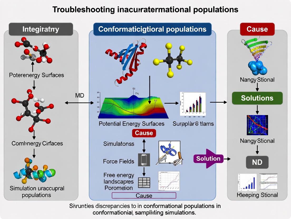
Diagram 1: Troubleshooting Inaccurate Conformational Populations
Troubleshooting Inaccurate Conformational Populations
Diagram 2: The Energy Landscape and Sampling Problem
The Energy Landscape and Sampling Problem
Diagram 3: Dynamic Cross-Correlation Network Analysis Workflow
Dynamic Cross-Correlation Network Analysis Workflow
The Scientist's Toolkit: Research Reagent Solutions
Table 4: Essential Software and Analysis Tools
| Tool Name | Function | Use Case |
|---|---|---|
| GROMACS | MD simulation software [20] | Performing high-performance MD simulations [20] |
| AMBER | MD simulation software [6] | Performing MD and aMD simulations [6] |
| NAMD | MD simulation software [6] | Performing MD simulations, particularly scalable on parallel computers [6] |
| Bio3D (R Package) | Analysis of biomolecular simulation data [20] | Calculating dynamic cross-correlation matrices (DCCM) [20] |
| MD-TASK | Suite for coarse-grained analysis of MD simulations [22] | Dynamic residue network analysis and perturbation-response scanning [22] |
| MODE-TASK | Suite for essential dynamics and normal mode analysis [22] | Analyzing global motion and conformational changes [22] |
Troubleshooting Guide: Force Field Selection and Validation
FAQ: How do I choose an appropriate force field for simulating Intrinsically Disordered Proteins (IDPs)?
The Challenge: Most traditional molecular dynamics (MD) force fields were developed and parameterized for folded, globular proteins. When applied to IDPs, they tend to overestimate intramolecular attraction, leading to overly compact structures that don't match experimental observations [23].
Troubleshooting Steps:
- Identify Protein Class: First, determine if your protein is fully disordered, contains disordered regions, or is a folded protein on the verge of disorder (like some LEA proteins) [23].
- Select Specialized Force Fields: For IDPs, prefer force fields specifically developed or optimized for disordered states. These often modify protein-water interactions or torsion parameters to improve hydration and conformational sampling [23].
- Run Short Validation Simulations: Perform multiple short (e.g., 200 ns) simulations from different initial structures to assess convergence and compare against available experimental data [23].
- Validate Against Experimental Data: Compare simulation results with Small-Angle X-Ray Scattering (SAXS) data for general compactness and Nuclear Magnetic Resonance (NMR) data for local structural features and dynamics [23].
Performance Table of Selected Force Fields for IDPs (COR15A Case Study) [23]:
| Force Field | Water Model | Performance Summary for IDPs (COR15A) |
|---|---|---|
| DES-amber | TIP4P-D38 | Best overall performance; captured helicity differences between WT and mutant and adequately reproduced NMR relaxation dynamics [23]. |
| ff99SBws | TIP4P/2005s | Captured helicity differences but overestimated overall helicity; reasonable performance for structural properties [23]. |
| ff99SB-disp | a99SB-disp | Performance varies; requires validation against specific experimental data for your system [23]. |
| CHARMM36m | mTIP3P/TIP4P | Improved for IDPs over earlier CHARMM versions, but may still over-stabilize certain secondary structures in some sequences [23]. |
| OPLS-AA | TIP4P | Not recommended for IDPs without modification; tends to overestimate compactness [23]. |
FAQ: My simulations of a globular protein show unrealistic structural drift. Is this a force field issue?
The Challenge: Even for globular proteins, force field choice is critical. Some force fields may introduce instabilities in loops, secondary structures, or at binding sites, leading to unrealistic deformation during simulation.
Troubleshooting Steps:
- Verify Starting Structure Quality: Ensure your initial model is high-quality. MD refinement works best for fine-tuning reliable models, not correcting poor ones [24].
- Check Simulation Stability: Monitor Root-Mean-Square Deviation (RMSD) and potential energy during an equilibration period. The RMSD should plateau, indicating the simulation has reached characteristic conformational sampling [23].
- Optimize Simulation Length: For refinement of already-good models, short simulations (10-50 ns) are often sufficient. Longer simulations (>50 ns) can induce structural drift and reduce fidelity to the experimental starting structure [24].
- Use a Standard Benchmark: Test your force field on a well-characterized globular protein with known experimental dynamics to establish a performance baseline before applying it to your protein of interest.
FAQ: How can I validate my force field choice against experimental data?
The Challenge: Force field performance can be system-dependent. Rigorous validation is required to ensure your simulations accurately reflect reality.
Validation Protocol:
- Compare Global Properties: Calculate the radius of gyration (Rg) or the pair distribution function P(r) from your simulation ensemble and compare it to SAXS data [23].
- Validate Local Structure: Calculate chemical shifts or J-couplings from simulations and compare to NMR data. For IDPs, ensure the force field can capture subtle structural differences, such as those caused by point mutants [23].
- Check Dynamic Properties: Compare order parameters or NMR relaxation times derived from simulations with experimental NMR data to assess if the dynamics are accurately reproduced [23].
- Two-Step Approach: Consider an initial screening with short simulations (e.g., 200 ns) against SAXS data, followed by extended simulations (e.g., 1+ μs) of the best-performing models for detailed validation against NMR data [23].
Diagram 1: Force field selection and validation workflow for troubleshooting conformational populations.
Key Research Reagent Solutions
Specialized Force Fields for Biomolecular Simulations:
| Reagent/Resource | Function & Application | Key Considerations |
|---|---|---|
| DES-amber | An IDP-optimized force field. Best for capturing conformational landscapes and dynamics of disordered proteins, as validated for COR15A [23]. | Use with TIP4P-D38 water model. Excellent for proteins on the verge of folding. |
| ff99SBws | A water-scaling force field for IDPs. Reduces protein-protein interactions to prevent overly compact structures [23]. | May overestimate secondary structure propensity (e.g., helicity) in some systems [23]. |
| CHARMM36m | A modern, widely used force field updated for both folded proteins and disordered systems [25]. | A good general-purpose choice, but always validate for your specific protein. |
| Amber with χOL3 | RNA-specific force field. Recommended for RNA structure refinement and stability testing in MD simulations [24]. | Used in CASP15 RNA refinement benchmarks. Best for fine-tuning reliable RNA models [24]. |
Critical Databases for Dynamic Conformational Data:
| Database | Content & Application | Access Link |
|---|---|---|
| ATLAS | MD simulations of ~2000 representative proteins for protein dynamics analysis [25]. | https://www.dsimb.inserm.fr/ATLAS |
| GPCRmd | MD trajectories focused on G Protein-Coupled Receptors for functionality and drug discovery [25]. | https://www.gpcrmd.org/ |
| SARS-CoV-2 DB | MD simulations of coronavirus proteins to support drug discovery [25]. | https://epimedlab.org/trajectories |
Experimental Protocols
Protocol 1: Initial Force Field Screening for IDPs
This protocol is adapted from the systematic comparison study of COR15A [23].
1. System Preparation:
- Generate 10 independent initial structures for your protein to sample different starting conformations.
- Solvate the protein in a cubic water box with at least 38,000 water molecules.
- Add ions (e.g., 6 Na⁺) to neutralize the system charge.
2. Simulation Setup:
- Test a panel of force fields (e.g., DES-amber, ff99SBws, CHARMM36m, etc.) with their recommended water models.
- Use a thermostat like Bussi-Donadio-Parrinello (BDP) with a coupling constant (τT) of 0.1 ps.
- Use a barostat like Parrinello-Rahman (PR) with a coupling constant (τp) of 2.0 ps.
3. Production and Analysis:
- For each force field, run 10 independent simulations of 200 ns from the different initial structures.
- Treat the first 120 ns as an extended equilibration period. Use only the final 80 ns for production analysis [23].
- Calculate the radius of gyration (Rg) and compare the average against experimental SAXS data to identify the best-performing force fields.
Protocol 2: MD Refinement for RNA Structures
This protocol is based on the CASP15 RNA refinement benchmark [24].
1. Input Model Selection:
- Crucial Step: This method is only effective for high-quality starting models. MD refinement can provide modest improvements by stabilizing stacking and non-canonical base pairs. Poorly predicted models rarely benefit and often deteriorate [24].
- Use models from accurate prediction tools as a starting point.
2. Simulation Execution:
- Use the Amber suite with the RNA-specific χOL3 force field.
- Run short simulations of 10-50 ns. Early dynamics (first few ns) reveal the model's stability and refinement potential.
- Avoid long simulations: Simulations longer than 50 ns typically induce structural drift and reduce model fidelity [24].
3. Analysis:
- Monitor the stability of base pairs and stacking interactions.
- Use metrics like RMSD to assess if the simulation is refining or distorting the initial model. The goal is fine-tuning, not large-scale correction [24].
Diagram 2: MD refinement protocol for improving high-quality RNA models.
Advanced Sampling and Integrative Methods for Accurate Ensembles
Frequently Asked Questions (FAQs)
Q1: What are the primary causes of inaccurate conformational populations in MD simulations? Inaccurate conformational populations primarily stem from two sources: insufficient sampling of conformational space due to limited simulation timeframes and inaccuracies in the molecular mechanics force fields used to describe atomic interactions. Even with enhanced sampling, the accuracy of the resulting ensembles is highly dependent on the quality of the physical models, or force fields, used. Discrepancies between simulations run with different state-of-the-art force fields can persist, leading to varying conformational distributions [26].
Q2: How can I integrate experimental data to improve the accuracy of my conformational ensembles? Integrative approaches, such as maximum entropy reweighting, allow you to refine computational ensembles with experimental data. This method introduces the minimal perturbation to a computational model required to match a set of experimental data, such as NMR spectroscopy and Small-Angle X-Ray Scattering (SAXS) data. This combines the atomistic detail of simulations with the validation provided by experimental observables, helping to achieve force-field independent conformational ensembles [26].
Q3: My λ-dynamics simulation is not sampling chemical space effectively. What could be wrong? Ineffective sampling in λ-dynamics can occur if the biasing potentials in λ-space are not optimal. A technique called Adaptive Landscape Flattening (ALF) can be used to find optimal fitting parameters for the λ-dependent biasing potentials, which helps to flatten the free energy landscape in λ-space and enables adequate sampling of different chemical species. It's important to note that while an optimal bias is beneficial, it is not always strictly necessary to achieve sufficient sampling [27].
Q4: What is a robust method for estimating statistical errors in my simulation results? For statistically robust error estimation, especially when dealing with correlated data from MD trajectories, it is recommended to use a combination of multiple independent simulations and block averaging [28].
- Run multiple independent simulations (e.g., 100 runs) with different initial seeds.
- For each simulation, use block averaging to compute the mean of the quantity of interest and its statistical error, which accounts for serial correlations within the trajectory.
- The final estimate is the average of the means from all simulations, with the final error calculated by propagating the individual errors from each simulation (e.g., standard error propagation assuming independent errors) [28].
Q5: I am getting "atom not found in residue topology database" errors when setting up my system. How do I resolve this?
This error in tools like GROMACS's pdb2gmx indicates that the residue or molecule you are trying to simulate is not defined in the chosen force field's database. Your options are to:
- Check for naming: See if the residue exists in the database under a different name and rename your molecule accordingly.
- Use a different force field: Another force field may already have parameters for your molecule.
- Find existing parameters: Search the literature for published parameters compatible with your force field.
- Parameterize it yourself: Create the topology and parameters for the new molecule, which is a complex task even for experts [29].
Troubleshooting Guides
Guide: Troubleshooting Force Field Inaccuracies and Ensemble Errors
Problem: Your simulated conformational ensemble does not agree with experimental data, such as NMR chemical shifts, SAXS profiles, or order parameters.
Diagnosis and Solutions:
Step 1: Validate against experimental data.
- Action: Compare your simulation's back-calculated observables (e.g., NMR chemical shifts, relaxation rates, SAXS intensities) directly to experimental values. Do not rely solely on structural intuition.
- Protocol: Use tools like
ABSURDerror implement a maximum entropy reweighting protocol to quantitatively assess the agreement. A significant mismatch indicates either insufficient sampling or force field inaccuracy [26] [30].
Step 2: Apply integrative structural biology methods.
- Action: If a reasonable initial agreement exists but is not perfect, use experimental data to refine your ensemble.
- Protocol: Employ a maximum entropy reweighting procedure. This statistical method reweights the frames of your MD simulation so that the averaged back-calculated observables match the experimental data, with minimal perturbation to the simulated ensemble [26].
- Workflow:
- Run a long, unbiased MD simulation or use an enhanced sampling method to generate a diverse conformational ensemble.
- For each frame in the trajectory, use a forward model to calculate the expected experimental observable (e.g., chemical shift).
- Use a maximum entropy algorithm to determine new statistical weights for each frame so that the reweighted ensemble averages match the experiment.
- Use the Kish ratio to ensure the effective ensemble size remains large enough to be statistically representative and avoid overfitting [26].
Step 3: Test multiple force fields.
- Action: The accuracy of MD simulations is highly force-field dependent. If reweighting fails or the initial agreement is poor, the force field may be the source of error.
- Protocol: Run comparable simulations with different, modern force fields (e.g., a99SB-disp, CHARMM36m, CHARMM22*) and compare their inherent agreement with experimental data before reweighting. Studies show that ensembles from different force fields can converge to highly similar distributions after reweighting with sufficient experimental data, providing a more force-field independent result [26].
Guide: Troubleshooting Sampling Issues in Alchemical and λ-Dynamics
Problem: Poor sampling of ligand binding modes or inefficient exploration of chemical space in alchemical methods like λ-dynamics.
Diagnosis and Solutions:
Solution 1: Implement advanced λ-dynamics frameworks.
- Problem: You need to compute free energy landscapes for multiple chemical species (e.g., different ligands or mutations) and find running separate simulations for each one inefficient.
- Protocol: Use the
MSλD+USframework, which combines umbrella sampling (US) with multisite λ-dynamics [27]. - Workflow:
- System Setup: Represent multiple ligands explicitly in a single simulation system, tethered together by harmonically restraining their common core atoms.
- Run Coupled Simulation: In each umbrella sampling window, run a λ-dynamics simulation. The λ variables, which control the alchemical state, are treated as dynamic variables with their own mass and can evolve continuously in response to the environment.
- Apply Biasing Potentials: Use a set of λ-dependent biasing potentials (
U_fixed,U_quadratic,U_end,U_skew) to discourage unphysical states and improve sampling. Optimize these biases using Adaptive Landscape Flattening (ALF) before production runs [27]. - Analysis: Use the Multistate Bennett Acceptance Ratio (MBAR) to recover the potential of mean force (PMF) for each chemical species from the single, combined simulation [27].
Solution 2: Use Grand Canonical Monte Carlo for fragment binding.
- Problem: Spontaneous binding of fragments in standard MD is too rare, and identifying multiple binding modes is difficult.
- Protocol: Employ Grand Canonical Nonequilibrium Candidate Monte Carlo (GCNCMC) [31].
- Workflow:
- Define Region: Specify the region of interest on the protein where fragments can be inserted or deleted.
- Propose Moves: Randomly attempt insertion, deletion, or movement of fragments within the region.
- Nonequilibrium Switching: Each insertion or deletion move is performed gradually over several alchemical steps, allowing the protein and solvent to adapt (induced fit).
- Monte Carlo Test: The proposed move is accepted or rejected based on the Metropolis criterion, ensuring sampling of the grand canonical ensemble.
- Benefit: This method efficiently finds occluded binding sites, samples multiple binding modes, and can calculate binding affinities without the need for complex restraints [31].
Guide: Resolving Common Software Errors in GROMACS
Problem: Energy minimization fails with "Energy minimization has stopped because the force on at least one atom is not finite. This usually means atoms are overlapping." [32]
Diagnosis and Solutions:
Step 1: Identify the problematic atom.
- Action: The error log will specify the atom number (e.g., "Fmax= inf, atom= 1251"). Use visualization software (e.g., VMD, PyMOL) to inspect this atom and its immediate environment for severe clashes, often with other parts of the protein, ligand, or solvent [32].
Step 2: Check for topology-coordinate mismatch.
- Action: This is a common cause. The atom names and/or residue names in your coordinate file (e.g.,
.groor.pdb) must exactly match those defined in your topology file (.top/.itp). - Protocol: Manually compare the atom names in the ligand's residue in the coordinate file against the definition in the force field residue topology database (
.rtp) or your ligand's.itpfile. Correct any naming discrepancies [29] [32].
- Action: This is a common cause. The atom names and/or residue names in your coordinate file (e.g.,
Step 3: Manually resolve clashes.
- Action: If the topology is correct, the structure itself may have overlapping atoms.
- Protocol:
- Slightly shift the position of the offending ligand or residue to eliminate the clash.
- Use a molecular modeling program like MOE or Chimera to perform a quick, preliminary energy minimization on the problematic region before setting up the GROMACS simulation [32].
Problem: grompp fails with "Invalid order for directive..." [29]
Diagnosis and Solutions:
- Cause: The directives in your topology (
.top) and include (.itp) files must appear in a specific order, as defined by GROMACS. - Solution: Restructure your topology file. The general order is:
[ defaults ][ atomtypes ][ moleculetype ](for the entire system)[ system ][ molecules ]
- Ensure that all
[ *types ]directives (e.g.,[ atomtypes ],[ bondtypes ]) appear before the first[ moleculetype ]directive. This means force field parameters must be fully defined before any molecules are described [29].
Problem: grompp fails with "Found a second defaults directive" [29]
Diagnosis and Solutions:
- Cause: The
[ defaults ]directive appears more than once in your topology, which is invalid. - Solution: The
[ defaults ]should only be set once, typically when you#includeyour main force field. If you are including other.itpfiles (e.g., for a ligand) that contain their own[ defaults ]section, comment out or delete the redundant[ defaults ]directives in those secondary files [29].
Research Reagent Solutions
This table details key computational tools and methods used in advanced enhanced sampling studies.
Table 1: Key Research Reagents and Computational Tools
| Item Name | Function/Brief Explanation | Example Application Context |
|---|---|---|
| Maximum Entropy Reweighting | A statistical method to refine MD ensembles by minimally adjusting frame weights to match experimental data [26]. | Correcting inaccurate conformational populations in IDP simulations to match NMR data [26]. |
| Multisite λ-Dynamics (MSλD) | An alchemical method that allows multiple chemical species (e.g., different ligands) to be simulated simultaneously in a single system by treating λ as a dynamic variable [27]. | Efficiently computing PMFs for multiple ligands binding to a protein from one set of simulations [27]. |
| Grand Canonical NCMC (GCNCMC) | A Monte Carlo method that allows for the insertion and deletion of molecules in a defined region during an MD simulation, facilitating the discovery of binding sites and modes [31]. | Identifying fragment binding sites and multiple binding modes in fragment-based drug discovery [31]. |
| Umbrella Sampling (US) | An enhanced sampling technique that uses harmonic biases along collective variables (CVs) to force the system to sample high-energy states and reconstruct free energy profiles [27]. | Calculating the potential of mean force for processes like ligand unbinding or protein folding [27]. |
| Adaptive Landscape Flattening (ALF) | An automated procedure to optimize the biasing potentials in λ-dynamics simulations, which improves the sampling efficiency in λ-space [27]. | Overcoming poor sampling of different chemical states in a multisite λ-dynamics simulation [27]. |
| Multistate Bennett Acceptance Ratio (MBAR) | A statistically optimal method for analyzing data from multiple equilibrium samples (e.g., from umbrella sampling) to compute free energies and PMFs [27]. | Recovering unbiased free energy profiles from a set of biased umbrella sampling simulations [27]. |
Workflow and Relationship Visualizations
The following diagram illustrates the integrative workflow for determining accurate conformational ensembles, combining molecular dynamics simulations with experimental data.
Integrative Workflow for Conformational Ensembles
This diagram outlines the protocol for using advanced λ-dynamics to simultaneously study multiple chemical species.
MSλD+US Protocol for Multiple Species
Leveraging True Reaction Coordinates for Efficient Barrier Crossing
Troubleshooting Guide: Identifying and Validating Reaction Coordinates
This guide addresses common challenges researchers face when identifying True Reaction Coordinates (tRCs) and their impact on obtaining accurate conformational populations in Molecular Dynamics (MD) simulations.
Table: Troubleshooting Common RC-Related Problems
| Problem Symptom | Potential Cause | Diagnostic Steps | Solution & References |
|---|---|---|---|
| 1. Ineffective Enhanced Sampling: Biased simulations show no significant acceleration of conformational changes. | Hidden Barriers: The biased Collective Variables (CVs) are orthogonal to the true reaction coordinates, leaving the actual activation barrier unsampled [33]. | Perform a committor analysis on configurations with the biased CV held at its transition state value. A broad committor distribution indicates a poor RC [34]. | Re-identify CVs using methods that target the committor, such as the generalized work functional (GWF) method [35]. |
| 2. Non-Physical Trajectories: Accelerated transition paths deviate from expected mechanistic understanding. | Incorrect Collective Variables: Empirically chosen CVs (e.g., RMSD, principal components) do not capture the essential dynamics of the process [33] [35]. | Compare the biased trajectory pathway to a known natural reactive trajectory (NRT) or experimental data. Check for unrealistic atomic clashes or geometries [35]. | Replace intuitive CVs with tRCs identified via physics-based methods like energy flow theory, which generate natural transition pathways [33] [35]. |
| 3. Force Field Dependent Results: Conformational ensembles differ significantly when using different force fields. | Incomplete Sampling & Force Field Bias: Under-sampling combined with inherent force field inaccuracies leads to ensembles trapped in different local minima [26] [36]. | Validate the unbiased simulation ensemble against multiple experimental observables (NMR, SAXS). Use the Kish ratio to check for effective ensemble size after reweighting [26]. | Integrate simulations with experimental data using maximum entropy reweighting to obtain force-field independent conformational ensembles [26]. |
| 4. Failure to Generate Transition Paths: Transition path sampling (TPS) cannot find an initial reactive trajectory or transition state configurations. | High Barrier & Rare Events: The system is trapped in the reactant basin, and no initial transition state conformation is available to seed TPS [35]. | Attempt to compute committor values from the reactant basin; a value of exactly 0 confirms the system is trapped. | Use enhanced sampling biased on pre-computed tRCs to efficiently generate trajectories that pass through the transition state region (pB~0.5), providing initial states for TPS [35]. |
Frequently Asked Questions (FAQs)
Q1: What is the fundamental difference between a collective variable (CV) and a true reaction coordinate (tRC)?
A CV is any function of atomic coordinates used to describe the progress of a process. A tRC is a special type of CV that exactly determines the committor probability for any given system configuration [35]. While many CVs can be proposed, only a tRC guarantees that the dynamics projected onto it will correctly describe the reaction mechanism and kinetics. Using a non-optimal CV leads to the "hidden barrier" problem, whereas biasing a tRC provides optimal sampling efficiency [33].
Q2: How can I objectively test if my proposed coordinate is a good reaction coordinate?
The most rigorous validation is the committor test (or committor histogram test) [34].
- Define your reactant (A) and product (B) states.
- Select configurations from your simulation where your proposed RC has a value corresponding to the transition state (e.g., the top of the free energy barrier).
- For each of these configurations, launch multiple, short, unbiased MD trajectories with random initial velocities.
- Calculate the committor, pB, as the fraction of trajectories that reach B before A.
If your proposed coordinate is a good RC, the histogram of pB values for these configurations will be sharply peaked at pB = 0.5. A broad histogram indicates the coordinate is insufficient [33] [34].
Q3: My enhanced sampling simulation converges to a free energy profile, but the predicted population of a key intermediate is inconsistent with experiment. What could be wrong?
This is a classic symptom of an inaccurate conformational ensemble. The issue may not be the free energy profile along your chosen CV, but rather that the conformational ensemble at each point along the CV is incorrect. This can be caused by:
- Force Field Inaccuracies: The physical model favors incorrect conformations [26] [36].
- Insufficient Sampling: The simulation is not long enough to explore the full conformational space orthogonal to your CV, leading to a biased ensemble.
Solution: Integrate experimental data directly into your ensemble using maximum entropy reweighting. This method minimally adjusts the weights of your simulation frames to match experimental observables (e.g., NMR chemical shifts, J-couplings, SAXS profiles), resulting in a more accurate and force-field independent conformational ensemble [26].
Q4: What are the latest methods for systematically identifying tRCs without relying on intuition?
Recent advances provide physics-based, systematic approaches:
- Energy Flow Theory and Generalized Work Functional (GWF): This method identifies tRCs as the optimal channels for energy flow during a conformational change. It calculates the Potential Energy Flow (PEF) through individual coordinates and uses GWF to generate an orthonormal set of "singular coordinates," with the tRCs being the ones with the highest PEFs [33] [35]. A key advantage is that tRCs can be computed from energy relaxation simulations, which are easier to perform than waiting for a rare reactive event [35].
- Machine Learning (ML) and Committor-Based Analysis: ML models can be trained to approximate the committor function directly from a large set of structural descriptors. The features most important to the ML model's prediction are strong candidates for the tRC [37] [34].
Experimental Protocols
Protocol 1: Identifying tRCs Using the Generalized Work Functional Method
This protocol is based on the method described in Nature Communications 16, 786 (2025) [35].
1. System Preparation:
- Start with a single protein structure (e.g., from AlphaFold or crystal structure).
- Solvate and equilibrate the system using standard MD protocols.
2. Energy Relaxation Simulation:
- Instead of running a long, unbiased MD and waiting for a rare event, initiate a short simulation from a structure of interest.
- The tRCs will govern the energy relaxation process. Collect snapshots and coordinate trajectories from this simulation.
3. Calculate Potential Energy Flows (PEF):
- For each coordinate ( qi ) (e.g., dihedral angle, distance), compute the PEF over a time interval using: ( \Delta Wi(t1, t2) = -\int{qi(t1)}^{qi(t2)} \frac{\partial U(\mathbf{q})}{\partial qi} dq_i ) where ( U(\mathbf{q}) ) is the potential energy of the system [35].
- This measures the energy cost of the motion of each coordinate.
4. Apply the Generalized Work Functional:
- The GWF algorithm is applied to the simulation data to generate a set of orthonormal singular coordinates (SCs).
- This transformation disentangles the coordinates, maximizing the PEF through individual SCs.
5. Identify tRCs:
- The SCs with the highest PEFs are identified as the tRCs. These are the few essential coordinates that control the conformational change and energy activation.
Protocol 2: Validating an RC with Committor Analysis
This is the gold-standard test for any proposed RC [33] [34].
1. Define Stable States:
- Clearly define the reactant (A) and product (B) basins in terms of your chosen RC or other structural metrics.
2. Harvest Putative Transition States:
- Run an umbrella sampling or metadynamics simulation biased along your proposed RC.
- From this simulation, select 50-100 configurations where the RC value corresponds to the maximum of the free energy barrier (the putative transition state).
3. Compute Committor Values:
- For each selected configuration:
- Randomize atomic velocities from a Maxwell-Boltzmann distribution.
- Launch 50-100 short, unbiased MD trajectories.
- For each trajectory, monitor whether it reaches state B or state A first.
- The committor ( p_B ) is the fraction of trajectories that commit to B.
4. Analyze the Histogram:
- Construct a histogram of all computed ( p_B ) values.
- A successful RC will yield a histogram sharply peaked at ( p_B = 0.5 ). A broad, non-peaked distribution (e.g., uniform between 0 and 1) indicates a poor RC.
The Scientist's Toolkit
Table: Essential Reagents and Methods for tRC Research
| Tool / Reagent | Function / Description | Key Application in tRC Studies |
|---|---|---|
| Committor (pB) | The probability that a trajectory initiated from a given configuration reaches the product before the reactant [33] [34]. | The definitive metric for validating a proposed reaction coordinate. The "true" RC is the coordinate that perfectly predicts pB [35]. |
| Energy Flow Theory | A physics-based framework that describes how energy flows through specific coordinates to drive conformational changes [33]. | Provides a physical interpretation of tRCs as the "optimal channels of energy flow" and forms the basis for the GWF method [33] [35]. |
| Generalized Work Functional (GWF) | A computational method that generates an orthonormal coordinate system to disentangle tRCs from other degrees of freedom [35]. | Used to systematically identify tRCs from simulation data by maximizing the potential energy flow through individual singular coordinates [35]. |
| Maximum Entropy Reweighting | A statistical framework to integrate MD simulations with experimental data by minimally adjusting conformational weights [26]. | Corrects for force field inaccuracies and insufficient sampling to generate accurate conformational ensembles for validating and studying tRCs [26]. |
| Transition Path Sampling (TPS) | A suite of algorithms to harvest true, unbiased reactive trajectories between two stable states [35]. | Generates Natural Reactive Trajectories (NRTs), which are essential for both testing tRCs and providing initial data for some tRC identification methods [35]. |
Method Comparison & Workflow
Table: Comparison of Key RC Identification Methods
| Method | Underlying Principle | Required Input | Strengths | Weaknesses |
|---|---|---|---|---|
| GWF / Energy Flow [35] | Physics of energy transfer; identifies coordinates with highest energy cost. | A single structure (for energy relaxation) or pre-computed NRTs. | High physical interpretability; can be predictive from a single structure. | Relatively new method; requires implementation of specialized analysis. |
| Committor-Based ML [37] [34] | Machine learning to approximate the committor function. | A large dataset of configurations with known committor values. | Systematically screens 1000s of candidate coordinates; no intuition needed. | Requires many expensive committor calculations to generate training data. |
| Dimensionality Reduction (e.g., TICA, DiffMap) [37] | Identifies the slowest degrees of freedom in a simulation. | Long, unbiased MD simulation data. | Good for initial exploration and identifying slow modes. | Identifies slow coordinates, which are not necessarily the tRCs for a specific process. |
FAQs: Addressing Common Challenges in Integrative Modeling
Q1: My molecular dynamics (MD) simulations of an intrinsically disordered protein (IDP) do not match my experimental NMR data. What could be wrong?
The discrepancy often stems from inaccuracies in the molecular mechanics force field used in the simulations. Force fields can have an imbalance between protein-protein and protein-water interactions, leading to conformations that are more compact or extended than in reality [38]. The recommended solution is to apply a maximum entropy reweighting procedure. This method uses your experimental NMR data to reweight the structures from your simulation, creating a new conformational ensemble that is consistent with both the simulation data and the experimental restraints, thereby correcting for force field inaccuracies [26].
Q2: How can I reliably combine sparse SAXS data with MD simulations without overfitting?
SAXS data has low information content (typically only 5-30 independent data points), making overfitting a significant risk [39]. To mitigate this, integrate SAXS data directly into your MD simulation as an energetic restraint using a method like SAXS-driven MD [39]. This approach uses the physical information encoded in the MD force field to restrain the simulation to conformations that are both physically realistic and compatible with the experimental SAXS curve. The force field acts as a powerful regularizer, greatly reducing the risk of overinterpreting the sparse data.
Q3: What does a "spiky baseline" in my NMR spectrum indicate, and how does it affect integrative modeling?
A spiky, somewhat symmetrical baseline in an NMR spectrum can be a sign of a mechanical failure in the NMR instrument, such as a malfunctioning lift on one of the magnet's legs [40]. This introduces vibrational noise into the data. For integrative modeling, which relies on high-quality, quantitative experimental data like NMR chemical shifts and paramagnetic relaxation enhancement (PRE), such artifacts can lead to incorrect calculation of conformational ensembles. Always collect data for standard compounds to verify instrument performance before conducting experiments for modeling [40].
Q4: How do I choose an initial structural model for a multidomain protein with flexible linkers when no single structure exists?
For flexibly linked multidomain proteins, an initial conformational ensemble can be generated using long-timescale, unbiased atomistic MD simulations [38]. Start the simulation from a structure where the individual domain structures are known (e.g., from crystallography or NMR) but are connected by the native linkers. The simulation will naturally sample various interdomain orientations. This ensemble can then be refined against experimental data such as SAXS and NMR PRE, which provide information on the overall shape and long-range distances, respectively [38].
Troubleshooting Guides for Specific Issues
Issue 1: Inaccurate Conformational Populations in IDP Ensembles
- Problem: The ensemble generated from MD simulation does not match the experimental radius of gyration (Rg) from SAXS or the NMR chemical shifts.
- Root Cause: The force field may inherently favor certain secondary structures or compactness over others, leading to a biased ensemble [26].
- Solution: Apply maximum entropy reweighting with extensive experimental datasets.
- Run long, unbiased MD simulations (microsecond scale) using a state-of-the-art force field [26].
- Collect extensive experimental data, including multiple NMR parameters (e.g., chemical shifts, J-couplings, PREs) and a SAXS profile [26].
- Use a robust reweighting protocol that automatically balances the restraints from all experimental datasets. A key parameter is the target effective ensemble size (Kish ratio, K), which helps prevent overfitting by ensuring a sufficient number of conformations contribute to the final ensemble [26].
- Validate the reweighted ensemble against experimental data not used in the reweighting.
Issue 2: Disagreement Between SAXS Data and Simulated Structures
- Problem: The theoretical SAXS curve back-calculated from your MD ensemble shows poor agreement with the experimental curve.
- Root Cause:
- Insufficient sampling of relevant conformations in the simulation.
- Inaccuracy in the forward model used to calculate the theoretical SAXS curve from atomic coordinates.
- Solution: Implement SAXS-driven MD simulations.
- Use an accurate forward model that accounts for the hydration layer and excluded solvent, as implemented in tools like GROMACS-SWAXS [39].
- Add an experiment-derived energy bias to the MD force field. This bias gently guides the simulation toward structures that minimize the difference (χ²) between the calculated and experimental SAXS curves [39].
- Run parallel replica simulations to refine a heterogeneous ensemble against the SAXS data, committing to the maximum entropy principle [39].
Issue 3: Refining a Multidomain Protein with Flexible Linkers
- Problem: Difficulty in determining the relative domain orientations due to a lack of interdomain restraints in experimental data.
- Root Cause: Traditional high-resolution methods like crystallography may not capture the full range of flexibility, and data from solution techniques like NMR may be sparse for defining domain arrangements [38].
- Solution: Integrate SAXS with NMR paramagnetic relaxation enhancement (PRE) and MD simulations.
- Perform PRE experiments by site-selectively attaching a paramagnetic spin label to one domain and measuring the effect on the NMR signals of the other domain. This provides long-range distance restraints [38].
- Collect SAXS data to obtain information on the overall shape and size of the molecule in solution [38].
- Construct a structural model by using the SAXS and PRE data to filter or bias conformational ensembles generated from microsecond-scale MD simulations. This integrated approach allows you to identify preferred interdomain orientations even in the absence of a fixed structure [38].
Workflow Diagrams for Integrative Modeling
Diagram 1: General Workflow for Integrative MD Refinement
General Workflow for MD Refinement
Diagram 2: Maximum Entropy Reweighting Procedure
Maximum Entropy Reweighting
Research Reagent Solutions
Table 1: Key Computational and Experimental Resources for Integrative Modeling
| Category | Item | Function in Integrative Modeling |
|---|---|---|
| Software & Tools | GROMACS-SWAXS [39] | A modified version of GROMACS for performing SAXS-driven MD simulations, using explicit-solvent SAXS calculations. |
| PLUMED [39] | A plugin for MD programs that can be used for metadynamics and other enhanced sampling methods, including SAXS-guided simulations. | |
| Bayesian/Maximum Entropy Reweighting Codes [26] [39] | Custom scripts (e.g., from GitHub repositories) to reweight MD ensembles using NMR and SAXS data based on maximum entropy or Bayesian inference principles. | |
| Force Fields | a99SB-disp [26] | A protein force field and water model combination noted for good performance in simulating IDPs and multidomain proteins. |
| CHARMM36m [26] | An improved force field for folded proteins and IDPs, often used with TIP3P water. | |
| CHARMM22* [26] | A force field used in benchmarking studies for IDP and protein simulations. | |
| Experimental Techniques | NMR Paramagnetic Relaxation Enhancement (PRE) [38] | Provides long-range distance restraints (up to ~25 Å) critical for defining the relative arrangement of domains in flexible proteins. |
| Small-Angle X-Ray Scattering (SAXS) [38] [41] | Provides low-resolution information about the overall shape, size, and flexibility of a biomolecule in solution. | |
| Site-Directed Spin Labeling [38] | Allows for the site-specific attachment of paramagnetic tags to proteins for PRE NMR experiments. |
Frequently Asked Questions
What is the primary goal of the Maximum Entropy Reweighting framework? The framework aims to refine molecular dynamics (MD) simulation ensembles by integrating experimental data. It seeks to produce a revised ensemble that agrees better with experiments while making the smallest possible perturbation to the original simulation, ultimately leading to conformational ensembles that are more accurate and independent of the initial force field used [42] [43] [26].
My reweighted ensemble fits the experimental data perfectly but looks unrealistic. What went wrong? This is a classic sign of overfitting [44]. It occurs when the reweighting is too aggressive, often due to an improperly chosen
θparameter that places excessive weight on fitting the data. To prevent this, use the χ² vs. Srel graph to select aθin the "balanced" region and monitor the Kish effective sample size to ensure a reasonable number of structures retain significant weight [44] [26].Can I use this framework even if my initial simulation is very different from the experimental data? The framework works best when your initial simulation has sampled conformations that are relevant to the true experimental ensemble. If the simulation is qualitatively wrong (e.g., it samples entirely the wrong secondary structures), reweighting may not be able to recover the correct ensemble. The method is most effective for refining ensembles, not for completely correcting a failed simulation [26].
What types of experimental data can be integrated? The framework is versatile and can incorporate data from various biophysical techniques, including:
How do I know if my final ensemble is accurate and trustworthy? A trustworthy ensemble should not only fit the experimental data used in the reweighting but also predict independent experimental data not used in the fitting process (validation data) [44]. Furthermore, when reweighting different MD force fields with sufficient data, they should converge to similar conformational distributions, indicating a force-field independent result [26].
Troubleshooting Guides
Poor Agreement After Reweighting
Problem: Even after reweighting, the calculated observables from the ensemble do not match the experimental data within the expected error.
- Potential Cause: Inaccurate forward model. The algorithm used to predict experimental observables (e.g., chemical shifts) from atomic coordinates may be biased or imprecise [44].
- Solution: Validate your forward model on a well-characterized system. Consider using secondary chemical shifts, which can cancel out some systematic errors in the predictor [44].
- Potential Cause: Insufficient sampling in the initial simulation. The initial MD ensemble may lack crucial conformations that are necessary to explain the experimental data.
- Solution: Extend your simulation time or run multiple independent simulations to improve conformational sampling. The reweighting method cannot create entirely new states [26].
- Potential Cause: Incorrect error estimation. The uncertainties (
σ_i) assigned to the experimental data or the forward model may be too small.- Solution: Re-evaluate your error estimates. The
σ_ivalues should reflect both experimental uncertainty and errors in the forward model [44].
- Solution: Re-evaluate your error estimates. The
Choosing the Hyperparameter θ
Problem: The balance parameter θ is difficult to choose, and its value strongly impacts the final results.
- Potential Cause: No systematic selection protocol. Choosing
θarbitrarily or based solely on the final χ² value can lead to overfitting or underfitting [44].- Solution: Use the validation-set method [44].
- Split your experimental data into a working set (used for reweighting) and a validation set (held out).
- Perform reweighting for a series of
θvalues. - For each
θ, calculate the χ² for both the working and validation sets. - Plot both χ² values against
θ. The optimalθis typically where the validation χ² is minimized, indicating a model that generalizes well.
- Solution: Use the validation-set method [44].
The table below summarizes the interpretation of different regions on a χ² vs. log(θ) plot:
Table: Interpreting the χ² vs. θ Relationship
| Region | θ Value | χ² Value | Srel Value | Interpretation | Risk |
|---|---|---|---|---|---|
| Overfitting | Low | Low | High | Excessive trust in experiment; large perturbation to simulation ensemble [44]. | Unphysical ensembles, poor generalization [44]. |
| Balanced | Intermediate | Moderately Low | Moderately Low | Good balance between experimental fit and prior information [26]. | Optimal for a robust, generalizable ensemble. |
| Underfitting | High | High | Low | Excessive trust in the initial simulation [44]. | Fails to improve agreement with experiment [44]. |
Ensemble Overfitting and Collapse
Problem: The reweighted ensemble is dominated by a very small number of conformations, leading to a loss of conformational diversity and potentially unphysical results [26].
- Potential Cause: The
θparameter is too low. This forces the algorithm to fit the experimental data exactly, often by assigning extremely high weights to a handful of structures [44].- Solution 1: Use the troubleshooting guide for choosing
θabove. - Solution 2: Monitor the Kish effective sample size (K) [26]. It is defined as K = (Σwᵢ)² / Σwᵢ², where wᵢ are the final weights. A sharp drop in K indicates ensemble collapse. In practice, you can set a threshold for K (e.g., 0.10) and choose
θaccordingly [26].
- Solution 1: Use the troubleshooting guide for choosing
Workflow and Methodology
The following diagram illustrates the typical workflow for applying the Maximum Entropy Reweighting framework, integrating the key steps and decision points discussed in the FAQs and troubleshooting guides.
Maximum Entropy Reweighting Workflow
Detailed Experimental Protocol: Bayesian/Maximum Entropy (BME) Reweighting [44] [43] [26]
- Generate Initial Ensemble: Perform long, unbiased MD simulations of your system (e.g., an Intrinsically Disordered Protein) using one or more force fields. Ensure the simulation is converged and has sampled a representative set of conformations.
- Prepare Experimental Data: Collect experimental data (e.g., NMR chemical shifts, SAXS profiles). Split the data into a working set and a validation set.
- Compute Prior Weights: For an unbiased simulation of N frames, the initial prior weight for each conformation is typically
w_j^0 = 1/N. - Apply Forward Model: For every frame in the MD ensemble, use an appropriate forward model (e.g., a chemical shift predictor) to calculate the theoretical value of each experimental observable.
- Scan θ Hyperparameter: Define a range of
θvalues (often on a logarithmic scale). For eachθvalue, solve the BME reweighting equation to obtain a new set of weights{w_j}that minimizes the function:L = χ²/2 - θ S_relwhereχ²measures the agreement with the working set data, andS_relis the relative entropy quantifying the perturbation from the initial ensemble [43]. - Select Optimal θ: For each
θ, compute the χ² for the validation set. Plot χ² (both working and validation) againstθ. Select theθvalue that minimizes the validation χ². - Produce Final Ensemble: Using the optimal
θ, compute the final weights{w_j}. This reweighted ensemble can now be used to compute other structural properties and validate against other independent data. - Assess Convergence: To claim a force-field independent ensemble, repeat this process with initial ensembles from different force fields. The reweighted ensembles should converge to highly similar conformational distributions [26].
The Scientist's Toolkit
Table: Essential Research Reagents and Resources
| Item / Resource | Function / Description | Example / Note |
|---|---|---|
| MD Simulation Software | Generates the initial conformational ensemble. | GROMACS [46], AMBER, CHARMM. |
| Experimental Data | Provides experimental restraints for reweighting. | NMR Chemical Shifts [44], SAXS data [26], HDX-MS [45]. |
| Forward Models | Calculates experimental observables from atomic coordinates. | Chemical shift predictors (e.g., SPARTA+, SHIFTX2) [44], SAXS profile calculators [26]. |
| Reweighting Software | Implements the BME algorithm to compute new weights. | Custom Python scripts (often available from GitHub repositories of cited papers) [43] [26]. |
| Force Fields | Defines the physical model for MD simulations. | a99SB-disp, CHARMM36m, AMBER03ws [44] [26]. |
| Validation Metrics | Tools to assess the quality and robustness of the reweighted ensemble. | Kish Effective Sample Size (K) [26], validation with unused data [44]. |
Frequently Asked Questions (FAQs)
Q1: My M&M simulation fails when restarting from a checkpoint file with a "particles communicated to PME rank are more than 2/3 times the cut-off" error. What should I do?
This is a common error indicating that your system may not be well-equilibrated or there is an issue with the restart configuration [47]. First, ensure you are using the correct grompp command to prepare the restart:
Then, in your .mdp file, set continuation = yes and gen-vel = no to continue from the stored state instead of re-initializing velocities [47]. If the problem persists, try running with increased -rdd (1.2) and -dds (0.9999) options in your mdrun command to allow more room for bonding interactions [47].
Q2: How can I assess and improve the accuracy of my conformational sampling in M&M?
Inaccurate conformational populations can arise from force field limitations or insufficient sampling. To quantify this, you can use experimental NMR chemical shifts as a benchmark [48]. Calculate the ensemble-averaged chemical shifts (e.g., for 1H, 15N, 13Cα) from your simulation trajectory using a Quantum Mechanical (QM) template-matching approach and compare them to experimental NMR data [48]. A significant deviation indicates potential force field inaccuracies or sampling issues. Consider using enhanced sampling techniques like metadynamics to improve exploration of conformational states [49].
Q3: What are the best practices for choosing an integration time step to minimize discretization errors?
Discretization errors are system-dependent and can significantly affect measured averages [50]. For a TIP4P water system at 300K, step sizes up to 7 fs (about 70% of the stability threshold) have been used successfully [50]. To determine the optimal step size for your system:
- Run short simulations with different time steps (e.g., 1, 2, 4 fs).
- Measure key quantities like potential energy, temperature components, and pressure.
- Plot these values against the time step; the region where they plateau indicates an acceptable step size with minimal discretization error [50]. Using a stochastic thermostat like Langevin can sometimes help manage these errors [50].
Troubleshooting Guides
Guide 1: Resolving Particle Distribution PME Errors
Particle Mesh Ewald (PME) errors often occur during restart of complex simulations like M&M [47]. Follow this workflow to resolve them.
Guide 2: Correcting Systematic Errors in Conformational Populations
Systematic errors in conformational populations can be identified and corrected by validating against experimental data [48].
Error Assessment and Solution Tables
Table 1: Common M&M Simulation Errors and Solutions
| Error Type | Symptoms | Possible Causes | Solutions |
|---|---|---|---|
| PME Redistribution [47] | Simulation fails on restart with "particles communicated to PME rank... more than 2/3 times the cut-off". | System not well-equilibrated; incorrect restart settings; domain decomposition issues. | Use continuation = yes; generate tpr with -t previous_run.cpt; add -rdd 1.2 to mdrun [47]. |
| Discretization Error [50] | Measured quantities (energy, temperature) drift with larger time steps; physical artifacts. | Integration time step is too large. | Reduce time step; extrapolate results from multiple step sizes; use stochastic thermostats [50]. |
| Systematic Coordinate Error [48] | Ensemble-averaged properties (e.g., chemical shifts) deviate from experimental NMR data. | Underlying force field inaccuracies; insufficient conformational sampling. | Use enhanced sampling (M&M); validate with QM-calculated chemical shifts; consider force field refinement [48]. |
| Lack of Sampling | Simulation trapped in a single conformational state; poor agreement with experimental ensemble data. | High energy barriers; short simulation time. | Apply metadynamics with appropriate Collective Variables (CVs); use replica exchange; increase simulation time [49] [51]. |
| Atom Type | QM Method (Recommended) | Reference Shielding (ppm) | Typical Error Threshold | Notes |
|---|---|---|---|---|
| 1H | DFT/B3LYP/6-311+G(2d,p) | 32.023 | > 3.2% | Highly sensitive to H-bonding electrostatics [48]. |
| 15N | DFT/B3LYP/6-311+G(2d,p) | 233.133 | > 1.5% | Useful for backbone conformation validation [48]. |
| 13Cα | DFT/B3LYP/6-311+G(2d,p) | 182.629 | > 1.9% | Good indicator of backbone torsional errors [48]. |
The Scientist's Toolkit: Research Reagent Solutions
Table 3: Essential Software and Validation Tools
| Tool Name | Function | Application in M&M |
|---|---|---|
| drMD [49] | Automated MD pipeline | Simplifies running production simulations and restarts; includes "first-aid" for failed runs [49]. |
| GROMACS-PLUMED [47] | MD engine with enhanced sampling | Core software for running Metadynamics Metainference simulations [47]. |
| Gaussian G09 [48] | Quantum Mechanical calculations | Calculates reference chemical shifts for error assessment of MD trajectories [48]. |
| CHEMSHIFT Protocol [48] | Template-based chemical shift assignment | Quantifies errors in backbone atoms by comparing simulation to NMR data [48]. |
| Modified Hamiltonian [50] | Backward error analysis | Interprets and corrects discretization errors from finite time steps [50]. |
A Practical Troubleshooting Protocol for Simulation Optimization
Troubleshooting Guides
How do I diagnose and overcome hidden energy barriers in conformational sampling?
Issue: Your molecular dynamics (MD) simulation appears trapped, failing to explore the full conformational landscape. This often manifests as a system unable to transition between biologically relevant states, leading to inaccurate conformational populations.
Diagnosis: This is a classic case of insufficient conformational sampling. The molecular system is trapped in local energy minima and cannot overcome energy barriers to explore the global conformational space [52]. This is particularly problematic for systems with high conformational diversity, such as Intrinsically Disordered Regions (IDRs) [52].
Solutions:
- Increase Sampling with Diverse Initial Conditions: Run a large number of standard (canonical) MD simulations starting from diverse initial conformations. While straightforward, this approach can be inefficient and the results may remain highly dependent on the starting structure [52].
- Employ Enhanced Sampling Methods: Utilize advanced algorithms designed to help the system overcome energy barriers.
- Replica-Exchange MD (REMD): This method runs multiple replicas of the system at different temperatures and periodically swaps configurations between them. This allows high-temperature replicas to cross barriers and guide low-temperature replicates to explore new states [52].
- Multicanonical MD (McMD): This method applies an artificial potential to flatten the energy landscape, encouraging the system to explore a wider range of conformations [52].
Important Considerations for Enhanced Sampling: These methods require careful parameterization. The quality of a REMD simulation, for example, depends on the total simulation length, the number of replicas, and the exchange frequency. There is no universal "gold standard" for these settings, so technical experience is crucial [52].
Experimental Protocol: Setting up a Replica-Exchange MD (REMD) Simulation
- System Preparation: Prepare your system (protein, solvent, ions) as for a standard MD simulation.
- Determine Temperature Range: Choose a temperature range that spans from your temperature of interest to a sufficiently high temperature that enables barrier crossing. The highest temperature must not denature the key structural elements of your system.
- Calculate Replica Distribution: Use tools within your MD software package (e.g., GROMACS, AMBER) to determine the number of replicas and their specific temperatures to ensure a good exchange probability (typically 20-30%).
- Configure Exchange Parameters: Set the frequency for attempting exchanges between adjacent replicas (e.g., every 100-200 steps).
- Equilibration: Briefly equilibrate each replica at its assigned temperature.
- Production Run: Run the REMD simulation, ensuring that all replicas are run concurrently and can communicate for exchange attempts.
- Analysis: Use the output to analyze the conformational ensemble and compute free energy landscapes. Check the replica exchange statistics to ensure proper sampling.
How can I identify and fix non-physical trajectories caused by force field inaccuracies?
Issue: Your simulation exhibits unphysical behavior, such as bond distortion, instability at finite temperatures, or failure to reproduce known material properties or phase transitions, even with adequate sampling.
Diagnosis: The root cause is likely inaccuracies in the interatomic potential, or force field, which defines how atoms interact [53]. Classical force fields may not capture the complexity of the potential energy surface, especially for processes involving bond breaking or formation.
Solutions:
- Validate with Known Properties: Before running production simulations, test the force field's ability to reproduce key system properties, such as lattice parameters, densities, and phonon spectra. Universal machine learning force fields (MLFFs) trained on specific density functional theory (DFT) data can inherit biases from the exchange-correlation functionals used, leading to failures in predicting dynamic properties like phase transitions [53].
- Consider Machine Learning Force Fields (MLFFs): MLFFs can offer quantum-mechanical accuracy with the computational efficiency of classical MD [53]. However, their performance in finite-temperature MD simulations must be validated.
- Fine-Tune Universal Models: For universal MLFFs, fine-tuning on a smaller, system-specific dataset computed with a more suitable DFT functional can restore predictive accuracy [53].
- Implement Reactive Force Fields: For simulations involving bond breaking, consider switching from harmonic bond potentials to reactive potentials. The Reactive INTERFACE Force Field (IFF-R), for example, replaces harmonic bonds with Morse potentials, enabling bond dissociation while maintaining the accuracy of the original force field. This approach is about 30 times faster than complex bond-order potentials like ReaxFF [54].
Experimental Protocol: Validating a Force Field with a Phase Transition Benchmark
This protocol uses the phase transition in PbTiO₃ (PTO) as a benchmark, as described in the search results [53].
- Obtain the Ground-State Structure: Perform a structural optimization of the tetragonal phase of your material using the force field. Calculate the lattice parameters and tetragonality (c/a ratio).
- Compare with Reference Data: Compare the optimized structure with results from established quantum mechanics methods (e.g., DFT with LDA, PBE, PBEsol functionals) or experimental data. A significant deviation indicates a potential force field bias [53].
- Check Dynamical Stability: Calculate the phonon spectrum of the optimized structure. The absence of imaginary frequencies confirms the structure is dynamically stable. Their presence suggests instability and potential force field issues [53].
- Run Finite-Temperature MD: Perform an MD simulation at a constant temperature and pressure (NPT ensemble) while heating the system through its known phase transition temperature (760 K for PTO).
- Monitor for Unphysical Behavior: Observe the simulation for signs of instability, such as unrealistic cell deformation or failure to transition. The failure of a universal MLFF to capture this realistic dynamic behavior indicates it may not be suitable for your production runs [53].
Frequently Asked Questions (FAQs)
Q: My ligand-protein docking fails for large, flexible ligands. Is this a sampling or a scoring problem? A: For large ligands with many rotatable bonds, conformational sampling has historically been a major challenge. However, evidence suggests that with sufficient computational resources, sampling can be adequately addressed. The bigger unmet challenge is now scoring—accurately ranking the generated conformations to identify the correct binding pose [55].
Q: What are some best practices for visualizing uncertainty in my molecular structures? A: When representing uncertainty (e.g., in conformational ensembles), avoid overloading standard visual channels like color or size. Instead, use feature lines with varied attributes. Perceptual studies suggest using blur, dashing, grayscale, sketchiness, or width of lines to effectively encode scalar uncertainty data without cluttering the visualization [56].
Q: Why is conformational sampling particularly important in computational studies of natural products? A: Natural products are often complex, flexible molecules. The quality and reliability of computational studies—predicting reactivity, molecular structure, or biological activity—are entirely dependent on undertaking a thorough conformer search. Inadequate sampling can lead to incorrect conclusions [57].
Q: My free energy simulations of molecules in lipid bilayers are inconsistent. What could be wrong? A: These simulations are prone to systematic sampling errors. Hidden barriers can occur during solute adsorption, insertion, and when crossing the bilayer center. These barriers are often associated with lipid headgroups. The choice of initial conformation can dramatically influence the results, and barriers at the bilayer center may be linked to the membrane's bending modulus [58].
Research Reagent Solutions
The table below lists key computational tools and methods referenced in this guide.
Table: Key Research Reagents and Computational Methods
| Item Name | Function/Brief Explanation |
|---|---|
| Replica-Exchange MD (REMD) | An enhanced sampling method that uses parallel simulations at different temperatures to overcome energy barriers [52]. |
| Machine Learning Force Fields (MLFFs) | Force fields that use machine learning to achieve quantum-mechanical accuracy at a lower computational cost [53]. |
| Reactive INTERFACE FF (IFF-R) | A reactive force field that uses Morse potentials instead of harmonic bonds to simulate bond breaking and failure [54]. |
| Harmonic Force Fields (CHARMM, AMBER, etc.) | Classical, non-reactive force fields using harmonic potentials for bonds; accurate for many systems but cannot model bond dissociation [54]. |
| Parallelized Incremental Docking (DINC) | A meta-docking approach that solves conformational sampling for large ligands by running multiple short, parallel docking instances [55]. |
Diagnostic Workflows and Technical Relationships
The following diagrams outline the logical workflows for diagnosing and addressing the two common failure modes discussed in this guide.
Frequently Asked Questions (FAQs)
FAQ 1: My simulations of an intrinsically disordered protein (IDP) do not match my experimental NMR data. Could the force field be the problem? Yes, this is a common issue. The accuracy of molecular dynamics (MD) simulations for IDPs is highly dependent on the quality of the force field. While recent force fields have improved, discrepancies with experimental data like NMR chemical shifts and SAXS profiles often remain [26]. A recommended troubleshooting step is to use an integrative approach. You can reweight your existing MD simulation trajectories against the experimental data using a maximum entropy procedure. This method minimally perturbs the computational model to match the experiments and can help determine a more accurate conformational ensemble without needing to run new simulations [26].
FAQ 2: When simulating protein-DNA complexes, the DNA rapidly deforms from its experimental A-form structure. How can I fix this? This instability is a known problem in several AMBER force fields (e.g., OL15, OL21, bsc1), which are biased toward B-DNA and underestimate the stability of A-form DNA [59]. The solution is to use a force field with refined parameters for DNA sugar puckering. The recently developed OL24 parameters for AMBER, for example, specifically target the deoxyribose dihedral potential to increase the stability of the north (N) puckering found in A-DNA. Switching to the OL24 force field should better model the A/B equilibrium in aqueous solution, DNA/RNA hybrids, and protein-DNA complexes [59].
FAQ 3: I am getting different results for the same protein when using different MD software packages with the same force field. Why? Differences can arise from factors beyond the force field itself. While the force field is critical, other elements such as the integration algorithms, treatment of long-range electrostatics, constraints on bonds involving hydrogen atoms, and the specific water model can significantly influence the outcome [36]. To troubleshoot, ensure you are using consistent "best practice" parameters for your specific software package as recommended by its developers. When comparing studies, it's important to note not just the force field, but also the MD software, water model, and other key simulation parameters [36].
FAQ 4: How do I know if a force field is suitable for simulating non-natural peptides like β-peptides? Standard protein force fields are often not parameterized for non-natural compounds. You should seek out force fields that have been explicitly extended and validated for your specific molecules. For β-peptides, for example, dedicated parameter sets exist for CHARMM, AMBER, and GROMOS families [60]. A comparative study found that a recently refined CHARMM force field extension performed best overall, accurately reproducing experimental structures for all tested β-peptides, while the performance of AMBER and GROMOS was more sequence-dependent [60].
Troubleshooting Guides
Problem 1: Inaccurate Conformational Populations in IDP Simulations
Issue: The conformational ensemble generated for an intrinsically disordered protein (IDP) from an MD simulation is inconsistent with experimental observables (e.g., NMR chemical shifts, SAXS data).
Diagnosis Flowchart:
Solution: Integrative Refinement via Maximum Entropy Reweighting This protocol refines an existing MD ensemble by integrating it with experimental data without introducing significant bias [26].
- Step 1: Acquire Inputs. You will need:
- An unbiased MD simulation trajectory of your IDP.
- Experimental data (e.g., NMR chemical shifts, J-couplings, SAXS profile).
- Step 2: Calculate Theoretical Observables. Use forward models (e.g., SHIFTX2 for chemical shifts) to predict the experimental observables from every frame (conformation) of your MD trajectory [26].
- Step 3: Apply Maximum Entropy Reweighting. Use a robust reweighting procedure to assign new statistical weights to each frame in your trajectory. The goal is to find the set of weights that provides the best agreement with the experimental data while minimizing the deviation from the original simulation (i.e., maximizing entropy).
- Step 4: Validate the Refined Ensemble. Check that the reweighted ensemble agrees with the experimental data used for refinement. It is also good practice to validate the ensemble against a separate set of experimental data that was not used in the reweighting. A successful refinement will yield a force-field independent conformational ensemble that robustly matches experiments [26].
Research Reagent Solutions:
| Reagent / Tool | Function in Protocol |
|---|---|
| MD Trajectory (e.g., from GROMACS, AMBER, NAMD) | Provides the initial, atomistic conformational ensemble to be refined [26]. |
| Experimental NMR & SAXS Data | Serves as the experimental restraint for reweighting [26]. |
| SHIFTX2 or related tool | Forward model to calculate NMR chemical shifts from structures [26]. |
| Maximum Entropy Reweighting Code (e.g., custom scripts) | Core algorithm that calculates new statistical weights for trajectory frames [26]. |
Problem 2: Instability of Non-B-DNA Conformations
Issue: In simulations of DNA or protein-DNA complexes, the DNA spontaneously and rapidly transitions from the experimental A-form to B-form, or fails to sample A-form at all when it is expected.
Diagnosis Flowchart:
Solution: Employ a Force Field with Refined Torsional Potentials The root cause is often an underestimation of the stability of north (N) sugar puckering, which is characteristic of A-DNA. The solution is to use a force field with corrected parameters [59].
- Step 1: Identify Your Force Field. Check if you are using an AMBER force field like OL15, OL21, or bsc1, which are known to have this bias [59].
- Step 2: Upgrade to a Refined Force Field. Switch to a force field that has been specifically parameterized to improve the A/B equilibrium. The OL24 force field is a direct refinement of OL21 that modifies the δ sugar-phosphate backbone torsion and τ1 deoxyribose ring torsion parameters, leading to increased stability of the A-form [59].
- Step 3: Analyze Key Metrics. After running your simulation with the new force field, validate the results by monitoring:
Problem 3: Inaccurate Torsional Barriers in General Force Fields
Issue: A molecule, such as a drug-like small molecule or a non-natural amino acid, samples incorrect rotameric states due to inaccuracies in the underlying torsional potential.
Diagnosis Flowchart:
Solution: Refine Torsional Parameters Against Quantum Mechanical Data This guide outlines a general approach for refining torsional potentials, which has been successfully used for protein side-chains [61] and is the basis for modern parameterization [62].
- Step 1: Identify the Problematic Dihedral. Locate the specific torsion angle (e.g., a side-chain χ1 angle or a key ligand dihedral) whose population does not match experimental or expected chemical knowledge.
- Step 2: Generate Quantum Mechanical (QM) Reference Data. Perform a relaxed dihedral scan of the problematic angle using a high-level QM method (e.g., CCSD(T)/CBS estimate). This provides the target energy barrier and conformational energies [59] [61].
- Step 3: Parameterize New Torsional Terms. Fit the parameters of the MM dihedral potential to reproduce the QM energy profile. This can be done manually or using automated toolkits like Q-Force [62]. A modern approach is to move towards a "bonded-only" model for 1-4 interactions, which uses bonded coupling terms instead of scaled non-bonded interactions, leading to more accurate forces and potential energy surfaces [62].
- Step 4: Implement and Validate. Incorporate the new parameters into your force field and run validation simulations. For a protein, this could involve simulating a small helical peptide or a globular protein and comparing the rotamer distributions to those in the Protein Data Bank or against NMR J-couplings [61].
Force Field Comparison and Selection Guide
The table below summarizes the performance and application scope of various force fields discussed in the troubleshooting guides.
| Force Field | Primary Application Scope | Key Strengths | Known Limitations / Notes |
|---|---|---|---|
| a99SB-disp [26] | Intrinsically Disordered Proteins (IDPs) | Accurate conformational ensembles for IDPs; often used with maximum entropy reweighting [26]. | Water model (a99SB-disp water) is integral to its performance [26]. |
| CHARMM36m [26] [60] | Proteins, Nucleic Acids, IDPs | Good overall accuracy for folded proteins and IDPs; validated for diverse systems [26] [36]. | Performance can vary with simulation package and setup [36]. |
| OL24 [59] | DNA, Protein-DNA Complexes | Correctly models A/B DNA equilibrium; improved stability of A-form in complexes [59]. | Specific to DNA; pair with a suitable protein force field. |
| ff99SB-ILDN [61] | Proteins (Globular) | Improved side-chain torsion potentials (Ile, Leu, Asp, Asn); better agreement with NMR data [61]. | May be superseded by newer protein force fields for some applications. |
| CHARMM (β-peptide extension) [60] | Non-natural Peptides (β-peptides) | Accurately reproduces experimental structures of various β-peptides; derived from QM data [60]. | Specialized for β-peptides; requires compatible simulation software. |
Optimizing Collective Variables (CVs) to Accelerate Relevant Motions
This technical support center provides troubleshooting guides and FAQs for researchers facing challenges in optimizing collective variables (CVs) for molecular dynamics (MD) simulations, particularly within the context of correcting inaccurate conformational populations.
Frequently Asked Questions (FAQs)
FAQ 1: What are the most common symptoms of poorly chosen CVs in an enhanced sampling simulation?
You may be using suboptimal CVs if your simulations exhibit:
- Lack of Convergence: The free energy profile or key observables do not converge, even with long simulation times.
- Hysteresis: The system follows different paths when driven from state A to B versus from state B to A.
- Unphysical Trapping: The simulation becomes trapped in a metastable state that is not the true thermodynamic minimum.
- Poor Agreement with Experiment: The simulated conformational ensemble shows significant discrepancies when validated against experimental data, such as NMR chemical shifts or SAXS profiles [26].
FAQ 2: My simulation is biased with CVs but fails to match experimental data. How can I correct the conformational ensemble?
A powerful method is Maximum Entropy Reweighting [26]. This integrative approach minimally adjusts the statistical weights of frames from an unbiased or biased MD simulation to maximize agreement with experimental data while minimizing the deviation from the original simulated ensemble. It is a post-processing step that can correct for force field inaccuracies or inadequate sampling without rerunning simulations [26]. A fully automated procedure has been demonstrated to yield accurate, force-field-independent conformational ensembles for intrinsically disordered proteins (IDPs) [26].
FAQ 3: I only know my system's stable states, not the transition path. How can I find good CVs?
You can use machine learning with a classification objective. The process involves [63]:
- Running short, unbiased simulations localized in each known metastable state (e.g., reactant and product).
- Calculating a broad set of physical descriptors (e.g., distances, angles) from these trajectories.
- Training a neural network (e.g., using Deep-LDA) to find the linear combination of descriptors that best distinguishes between the states. The output of the network serves as a data-driven CV that can discriminate between the states, providing a starting point for enhanced sampling [63].
FAQ 4: How can I check if my CVs are missing important degrees of freedom ("hidden barriers")?
A robust strategy is to analyze a preliminary enhanced sampling simulation to find its slowest degrees of freedom [63]. Methods like Deep-TICA (Time-lagged Independent Component Analysis) can be applied to a trajectory (even one biased with suboptimal CVs) to identify the slowest modes of the system [63]. If these slowest modes are not well captured by your currently biased CVs, they represent the hidden barriers. These newly identified modes can then be used as improved CVs in subsequent sampling.
Troubleshooting Guides
Problem: Inaccurate Conformational Populations in IDPs
Issue: The ensemble of an intrinsically disordered protein (IDP) generated by MD simulations does not match experimental observations from techniques like NMR or SAXS [26].
Diagnostic Checklist:
| # | Question | If "No," Potential Cause |
|---|---|---|
| 1 | Do your unbiased simulations with different state-of-the-art force fields (e.g., a99SB-*disp, Charmm36m) show reasonable initial agreement with a subset of experimental data? | The force field may be fundamentally inaccurate for your system. |
| 2 | Are you using a sufficient number and type of experimental restraints (e.g., chemical shifts, J-couplings, SAXS data) to characterize the ensemble? | The experimental dataset may be too sparse to constrain the ensemble effectively [26]. |
| 3 | When applying maximum entropy reweighting, does the Kish ratio (effective ensemble size) remain above a minimal threshold (e.g., K > 0.01)? | The simulation may not have sampled configurations consistent with the experiment, leading to overfitting. |
Solution: Apply Maximum Entropy Reweighting
Experimental Protocol [26]:
- Simulation: Run long, all-atom MD simulations of the IDP using one or more modern force fields.
- Data Calculation: Use forward models to predict experimental observables (e.g., chemical shifts, SAXS profiles) from every frame of the simulation trajectory.
- Reweighting: Optimize the weight of each simulation frame to maximize the agreement with the entire set of experimental data. This is done by minimizing a function that includes the chi-squared error against experiments and an entropy term that penalizes large deviations from the original weights.
- Validation: Analyze the reweighted ensemble to ensure it maintains structural diversity (via the Kish ratio) and agrees with experimental data not used in the reweighting.
Diagram 1: Maximum entropy reweighting workflow.
Problem: Failed Conformational Transition in a Folded Protein
Issue: When using steered MD (SMD) to drive a transition between two states, the protein deforms or does not reach the correct target conformation [64].
Diagnostic Checklist:
| # | Question | If "No," Potential Cause |
|---|---|---|
| 1 | Do your CVs include descriptors at multiple scales (e.g., large-scale hinge motion and local side-chain reorientation)? | The CV set may be insufficient to describe the transition mechanism [64]. |
| 2 | Is the steering speed (or force constant) low enough to allow for relaxed adaptation? | Excessive speed can cause unphysical deformation. |
| 3 | Have you validated that the chosen CVs can induce the transition without a target bias, using a method like TAMD? | The CVs may be correlated with, but not causative of, the transition [64]. |
Solution: Identify a Minimal Set of CVs
Experimental Protocol [64]:
- Define Candidate CVs: Based on the known states and low-resolution data (e.g., from smFRET or XL-MS), define a pool of candidate CVs. These often include interatomic distances, angles, and dihedral angles.
- Screen with SMD: Systematically perform SMD simulations, biasing different combinations of CVs toward their target values.
- Identify Success: A successful transition is one where the protein reaches the target state with minimal root-mean-square deviation (RMSD) and without structural disruption.
- Find Minimal Set: Determine the smallest set of CVs that reliably produces a successful transition. The study on T4 lysozyme found that a combination of interdomain hinge bending and key local side-chain reorientation CVs was necessary [64].
- Validate with TAMD: Use Temperature-Accelerated MD (TAMD) with the identified minimal CV set. In TAMD, the CVs are coupled to fictitious particles accelerated at a high temperature, allowing the system to explore its conformational landscape without a predetermined target. Successfully observing the transition with TAMD validates that the CVs are true reaction coordinates [64].
Diagram 2: Collective variable optimization cycle.
The Scientist's Toolkit: Research Reagent Solutions
Table 1: Essential software and computational tools for CV optimization and enhanced sampling.
| Tool Name | Function | Use Case in CV Optimization |
|---|---|---|
| PLUMED | A plugin for MD codes that enables a vast range of enhanced sampling methods and CV analysis [63]. | The primary platform for defining, applying biases to, and analyzing CVs in simulations. |
| MLCVS | A Python package for building data-driven collective variables using machine learning models like Deep-LDA and Deep-TICA [63]. | Training neural networks to create CVs from simulation data. |
| GROMACS | A high-performance MD simulation package widely used for biomolecular systems [65]. | Running the underlying MD simulations, patched with PLUMED for enhanced sampling. |
| PyTorch | An open-source machine learning library [63]. | Used within mlcvs to define and train neural network-based CV models, which can be exported for use in PLUMED. |
| Maximum Entropy Reweighting Code | Custom code (often in Python or C++) that implements the maximum entropy principle to reweight simulation ensembles [26]. | Correcting conformational populations a posteriori to match experimental data. |
AI and Deep Learning as Efficient Alternatives for Conformational Sampling
Molecular dynamics (MD) simulations have long been the cornerstone of computational structural biology, providing atomistic insights into protein dynamics. However, when studying intrinsically disordered proteins (IDPs) or complex conformational changes, traditional MD faces significant limitations. The sheer computational expense of simulating biological relevant timescales (microseconds to milliseconds) and the difficulty in sampling rare, transient states often prevents accurate characterization of conformational ensembles [66]. This sampling inadequacy directly leads to inaccurate conformational populations, limiting the predictive power of simulations for drug discovery and functional analysis. Artificial intelligence, particularly deep learning, offers transformative alternatives by leveraging data-driven approaches to efficiently explore conformational landscapes, overcoming many limitations inherent to physics-based simulations alone [66] [67].
Frequently Asked Questions: Core Technical Challenges
Q1: Why do my MD simulations consistently fail to capture known experimental conformational states?
This failure typically stems from insufficient sampling of the conformational landscape and force field inaccuracies. MD simulations are often trapped in local energy minima, especially when high energy barriers separate functionally relevant states [66] [26]. The computational expense of simulating beyond microseconds for complex systems makes comprehensive sampling practically challenging. Additionally, despite recent improvements, force fields may contain biases that disfavor certain biologically relevant conformations, particularly for intrinsically disordered proteins [26].
Troubleshooting Protocol:
- Validate with experimental data: Compare your simulation results with available NMR chemical shifts, SAXS profiles, or J-couplings to identify systematic deviations [26]
- Implement enhanced sampling: Consider Gaussian accelerated MD (GaMD) or other biased sampling methods to improve barrier crossing [66]
- Try multiple force fields: Compare results across different modern force fields (CHARMM36m, a99SB-disp) to identify force-field-specific biases [26]
- Integrate AI sampling: Use deep generative models to identify potentially missed conformational states
Q2: How can I distinguish meaningful conformational changes from thermal noise in my simulations?
Meaningful conformational changes typically involve coordinated motions of structural elements that persist beyond transient fluctuations. Traditional analysis like RMSD can be insufficient to detect functionally relevant but subtle conformational shifts [68].
Troubleshooting Protocol:
- Employ deep learning classification: Train or use pre-trained convolutional neural networks on distance maps to identify non-trivial conformational patterns [68]
- Analyze collective variables: Identify relevant order parameters that capture the biological motion of interest
- Use community detection: Apply graph-based analyses to identify correlated motions across residue networks
- Validate functional relevance: Check if identified conformations impact binding sites, catalytic residues, or allosteric networks
Q3: My generative AI model produces physically unrealistic protein conformations. What safeguards can I implement?
This common issue arises when models prioritize statistical patterns over physical constraints. Several validation layers should be implemented [67] [69].
Troubleshooting Protocol:
- Implement physics-based filters: Reject conformations with steric clashes, unrealistic bond lengths/angles, or improper torsion angles
- Incorporate energy evaluation: Use fast physical potentials (MM, GB/SA) to score generated structures and filter high-energy outliers
- Leverage pretrained models: Use AlphaFold2 or ESMFold to assess plausibility through pLDDT scores or confidence metrics
- Validate against experimental data: Ensure generated ensembles match available experimental observables (NMR, SAXS) [26]
- Implement iterative refinement: Use rejected conformations to retrain or fine-tune generative models
Technical Specifications & Performance Metrics
Table 1: Comparison of AI-Based Conformational Sampling Methods
| Method Category | Representative Methods | Largest Validated System | Computational Efficiency | Key Advantages | Key Limitations |
|---|---|---|---|---|---|
| Deep Generative Models | DiG, AlphaFlow, UFConf | 306 residues [67] | GPU-seconds to minutes [67] | Statistically independent samples; High scalability | Potential for physically unrealistic structures; Training data dependency |
| Coarse-grained ML Potentials | Majewski et al., Charron et al. | 189 residues (PPIs) [67] | Orders of magnitude faster than all-atom MD [67] | Smoother energy landscape; Transferable across proteins | Slower than classical force fields per step; Limited atomic detail |
| MSA Perturbation Methods | MSA subsampling, AFCluster | PDB-scale monomers [67] | Comparable to AlphaFold2 inference [25] | No MD training data required; Leverages evolutionary information | Limited to natural sequences; Conformational diversity may be restricted |
| Hybrid AI-MD Frameworks | Maximum Entropy Reweighting | 140 residues (α-synuclein) [26] | MD simulation + reweighting overhead | Integrates experimental data; Force-field independent ensembles [26] | Dependent on initial MD sampling quality |
| Large Language Models | MD-LLM-1 | 164 residues (T4 lysozyme) [70] | Fine-tuning + inference time | Discovers unseen conformational states; Sequential modeling | Not explicitly modeling thermodynamics/kinetics [70] |
Table 2: Quantitative Performance of AI Sampling Methods on Benchmark Systems
| Method | Aβ40 (40 residues) | drkN SH3 (59 residues) | ACTR (69 residues) | α-synuclein (140 residues) | Validation Metrics |
|---|---|---|---|---|---|
| a99SB-disp MD | Good agreement with NMR [26] | Captures residual helicity [26] | Reasonable initial agreement [26] | Moderate agreement [26] | NMR chemical shifts, SAXS, J-couplings |
| Charmm36m MD | Systematic deviations [26] | Overcompaction issues [26] | Force-field dependent biases [26] | Varying accuracy [26] | NMR chemical shifts, SAXS, J-couplings |
| Maximum Entropy Reweighting | Significant improvement after reweighting [26] | Converged ensembles across force fields [26] | High similarity after reweighting [26] | Force-field independent ensembles achievable [26] | Kish ratio (~0.10); Ensemble similarity metrics |
| Deep Generative Models | Not fully benchmarked | Not fully benchmarked | Not fully benchmarked | Partial validation (RBD domain) [67] | RMSF profiles, contact fluctuations, state recall |
Experimental Protocols & Workflows
Protocol 1: Maximum Entropy Reweighting for Force-Field Independent Ensembles
This protocol enables researchers to derive accurate conformational ensembles by integrating MD simulations with experimental data [26].
Step-by-Step Methodology:
- Perform extensive MD simulations: Generate long-timescale (≥30μs) all-atom MD simulations using multiple state-of-the-art force fields (a99SB-disp, CHARMM36m, CHARMM22*)
- Collect experimental data: Acquire extensive NMR data (chemical shifts, J-couplings, NOEs) and SAXS profiles
- Calculate experimental observables: Use forward models to predict experimental measurements from each MD frame
- Apply maximum entropy reweighting:
- Define the objective function to minimize: Σwᵢlnwᵢ + λΣ(Oᵢ⟨w⟩ - Oᵢexp)²
- Automatically balance restraint strengths based on target ensemble size
- Use Kish ratio threshold (K=0.10) to maintain sufficient effective sample size
- Validate convergence: Assess similarity of reweighted ensembles from different initial force fields
- Deposit ensembles: Share final ensembles through Protein Ensemble Database for community use
Key Technical Considerations:
- Optimal Kish ratio thresholds balance experimental agreement and ensemble diversity
- Automated balancing of restraints from different experimental sources prevents subjective weighting
- Convergence to similar ensembles from different force fields indicates robustness
Maximum Entropy Reweighting Workflow
Protocol 2: Deep Generative Modeling for Conformational Diversity
This protocol uses diffusion models to generate diverse conformational ensembles without extensive MD sampling [67] [69].
Step-by-Step Methodology:
- Data preparation and representation:
- Collect training data from PDB, MD simulations (ATLAS, GPCRmd), or experimental ensembles
- Represent structures as internal coordinates (torsion angles) or distance maps
- Normalize structural features for training stability
Model architecture selection:
- Choose appropriate generative architecture (diffusion models, VAEs, normalizing flows)
- Implement SE(3)-equivariant networks for physical consistency
- Condition generation on evolutionary information (MSAs) or sequence embeddings
Training procedure:
- Pre-train on PDB structures to learn protein structural grammar
- Fine-tune on target protein class or specific system of interest
- Implement progressive training for large systems
Sampling and validation:
- Generate statistically independent samples through iterative denoising
- Filter physically unrealistic structures using energy calculations
- Validate against experimental data when available
- Assess diversity through RMSD clustering and coverage metrics
Key Technical Considerations:
- Training on both PDB and MD data improves coverage of conformational states
- Physical constraints prevent generation of unrealistic geometries
- Multi-scale validation ensures biological relevance
Advanced Techniques & Integration Frameworks
Large Language Models for Conformational Discovery
The MD-LLM framework demonstrates how protein structures tokenized as discrete sequences can be processed by transformer architectures to predict conformational dynamics [70].
Implementation Workflow:
- Structural tokenization: Use FoldToken encoder to convert 3D coordinates to discrete token sequences
- Temporal sequencing: Format MD trajectories as rolling window sequences for next-conformation prediction
- Model fine-tuning: Adapt pre-trained Mistral 7B using Low-Rank Adaptation (LoRA) on system-specific data
- Conformational discovery: Use fine-tuned model for iterative generation beyond training distribution
- Structure decoding: Convert generated tokens back to 3D coordinates using FoldToken decoder
MD-LLM Conformational Discovery Workflow
Research Reagent Solutions: Essential Tools & Databases
Table 3: Critical Research Resources for AI-Enhanced Conformational Sampling
| Resource Name | Type | Primary Function | Access Information | Key Applications |
|---|---|---|---|---|
| ATLAS Database | MD Database | Provides simulations of ~2000 representative proteins | https://www.dsimb.inserm.fr/ATLAS [25] | Training generative models; Method benchmarking |
| GPCRmd | Specialized MD Database | GPCR-focused simulations for drug target insights | https://www.gpcrmd.org/ [25] | Membrane protein dynamics; Drug discovery |
| Protein Ensemble Database | Experimental Ensembles | Repository for validated conformational ensembles | PED access codes [26] | Method validation; Training data |
| FoldToken | Structural Representation | Encodes 3D structures as discrete tokens for LLMs | Integrated in MD-LLM framework [70] | Language model processing; Structure generation |
| MaxEnt Reweighting Code | Software Tool | Integrates MD with experimental data | https://github.com/paulrobustelli/BorthakurMaxEntIDPs_2024/ [26] | Ensemble refinement; Force-field validation |
| SARS-CoV-2 MD Database | Specialized MD Database | Coronavirus protein simulations for drug discovery | https://epimedlab.org/trajectories [25] | Viral protein dynamics; Therapeutic development |
Advanced Troubleshooting: Specialized Scenarios
Q4: How can I validate my AI-generated ensembles when experimental data is limited or unavailable?
This common scenario requires creative validation strategies when direct experimental comparison isn't possible.
Troubleshooting Protocol:
- Implement computational cross-validation:
- Compare with long-timescale MD simulations on smaller systems
- Use multiple AI methods and assess consensus predictions
- Perform leave-one-out validation on known conformational states
Leverage evolutionary information:
- Analyze conservation patterns in predicted flexible regions
- Correlate predicted dynamics with co-evolutionary couplings
- Compare with ANM or ENM normal mode analyses
Functional validation:
- Test if generated ensembles explain known functional properties
- Assess binding site accessibility across predicted conformations
- Check consistency with phylogenetic relationships
Q5: My generative model produces ensembles that lack the diversity observed in experiments. How can I improve coverage?
This indicates issues with model architecture, training data, or sampling strategy.
Troubleshooting Protocol:
- Architecture improvements:
- Increase latent space dimensionality in VAEs
- Adjust noise schedules in diffusion models
- Implement hierarchical generation strategies
Training data enhancements:
- Incorporate enhanced sampling simulations in training data
- Add synthetic diversity through data augmentation
- Balance training data to avoid mode collapse
Sampling optimization:
- Adjust temperature parameters for sampling stochasticity
- Implement cluster-based sampling to cover distinct states
- Use adversarial validation to identify undersampled regions
Future Directions & Emerging Solutions
The field of AI-enhanced conformational sampling is rapidly evolving, with several promising directions addressing current limitations. Hybrid approaches that integrate physical constraints with data-driven models show particular promise for maintaining physical realism while leveraging the sampling efficiency of deep learning [66] [69]. The development of foundation models for protein dynamics, trained on extensive MD datasets, could provide generalizable priors for specific systems [67]. Multi-scale methods that combine coarse-grained exploration with all-atom refinement offer pathways to study larger systems over longer timescales. Finally, active learning frameworks that iteratively guide simulations based on model uncertainty can optimize the use of computational resources for challenging sampling problems [71].
For researchers encountering persistent challenges with conformational sampling accuracy, the integration of multiple complementary approaches—combining AI-generated diversity with physical validation and experimental integration—provides the most robust path forward toward biologically meaningful ensembles.
Frequently Asked Questions
1. My simulation fails to sample biologically relevant conformational changes. What is the most common cause? The most common cause is insufficient sampling. Molecular dynamics simulations are often limited to nanosecond or microsecond timescales, which is frequently insufficient for a system to overcome the high free-energy barriers separating different potential energy minima, or stable conformations. A single, short simulation is very likely to get trapped in a local energy minimum and not represent the true conformational ensemble of the protein [6] [72].
2. How can I accelerate the sampling of rare conformational events? You can use enhanced sampling methods that are specifically designed to help systems cross energy barriers more efficiently. Popular and well-integrated methods include:
- Accelerated Molecular Dynamics (aMD): This method adds a non-negative bias potential to the true potential energy surface, which raises the energy level of the minima relative to the barriers. This allows the system to transition between states more readily without requiring advanced knowledge of the landscape [6].
- Weighted Ensemble (WE): This path-sampling strategy runs multiple parallel simulations and uses intermittent resampling to focus computational effort on rare events. It provides unbiased kinetics and is highly efficient for simulating processes like conformational changes and binding [73].
3. What are the critical checks for my starting structure before a simulation? A poor starting structure is a primary source of error. Your pre-simulation checklist should include [72]:
- Completeness: Check for and add any missing atoms, residues, or loops.
- Steric Clashes: Identify and minimize severe atomic overlaps.
- Protonation States: Assign the correct protonation states for all residues at your desired pH.
- Structural Distortions: Correct any unrealistic geometries introduced during the initial modeling.
4. I am simulating a protein with a ligand. How do I avoid errors in parameterization? The key is to ensure force field compatibility. Never mix parameters from different force fields (e.g., CHARMM and AMBER) unless they are explicitly designed to work together, as they use different functional forms and derivation methods. For small molecules, use toolkits like the Force Field Toolkit (ffTK) to generate parameters that are fully compatible with your chosen force field (e.g., CHARMM/CGenFF or GAFF for AMBER) [74] [72].
5. My simulation is stable, but how do I know if the results are physically meaningful? A stable simulation does not guarantee an accurate one. You must validate your simulation against experimental data where possible. Key validation metrics include [72]:
- Root-mean-square fluctuation (RMSF) compared to experimental B-factors from crystallography.
- Nuclear Overhauser Effect (NOE) distances and scalar coupling constants compared to NMR data.
- Comparison of calculated properties like diffusion coefficients or order parameters with experimental values.
Troubleshooting Guide: Inaccurate Conformational Populations
| Symptom | Potential Cause | Solution | Validation |
|---|---|---|---|
| Low conformational diversity, trapped in a single state. | Inadequate sampling; high energy barriers. | Implement enhanced sampling (aMD, WE) [6] [73]. Run multiple independent simulations with different initial velocities [72]. | Monitor multiple order parameters (e.g., RMSD, radius of gyration, salt-bridge distances) to confirm broader sampling. |
| Unphysical protein or ligand dynamics (e.g., distortion, unfolding). | Incorrect or incompatible force field parameters; poor initial structure. | Re-parameterize custom molecules (e.g., ligands) with a tool like ffTK [74]. Re-check structure preparation for clashes and protonation states [72]. | Visually inspect trajectories; verify that bonded and non-bonded energies remain stable and within expected ranges. |
| Failure to reproduce a known conformational change. | Insufficient simulation time or replicates; incorrect system setup (e.g., missing ions). | Increase simulation time and number of replicates. Use enhanced sampling to target the transition. Ensure the physiological environment (ionic concentration, membrane) is correctly modeled. | Compare with experimental data on the transition, if available. Use analysis like Principal Component Analysis (PCA) to identify the relevant motions [6]. |
| Erratic system behavior or simulation crash. | Incorrect time step; inadequate minimization/equilibration; Periodic Boundary Condition (PBC) artefacts. | Use a timestep of 2 fs with hydrogen mass repartitioning. Ensure minimization has converged and equilibration shows stable temperature, pressure, and energy [72]. Process trajectories to correct for PBC artefacts before analysis. | Check log files for energy and temperature stability. Use tools like gmx trjconv (GROMACS) or cpptraj (AMBER) to make molecules whole. |
The Scientist's Toolkit: Essential Software and Methods
| Tool Name | Primary Function | Key Application in Troubleshooting |
|---|---|---|
| Accelerated MD (aMD) [6] | Enhanced sampling by flattening energy barriers. | Accelerates transitions between protein conformational states when rare events are the problem. |
| Weighted Ensemble (WE) [73] | Path sampling for efficient simulation of rare events. | Provides unbiased kinetics and improves sampling of long-timescale processes like (un)binding. |
| Force Field Toolkit (ffTK) [74] | Parameterization of small molecules for CHARMM force fields. | Generates compatible and accurate parameters for ligands, cofactors, and other novel chemical matter. |
| Principal Component Analysis (PCA) [6] | Dimensionality reduction to identify large-scale motions. | Analyzes trajectories to pinpoint the essential collective movements associated with a conformational change. |
| Internal Coordinate Net (ICoN) [75] | Deep learning model for sampling conformational ensembles. | Rapidly generates diverse and thermodynamically stable conformations beyond the scope of initial MD data. |
Workflow for Diagnosing Conformational Sampling Issues
The following diagram outlines a systematic workflow for troubleshooting inaccuracies in conformational populations.
Benchmarking and Validating Your Conformational Ensemble
Frequently Asked Questions (FAQs)
Q1: What is the Kish Ratio, and why is it important for analyzing my conformational ensemble?
The Kish Ratio (K) is a statistical metric that measures the effective sample size of a reweighted molecular dynamics ensemble. It quantifies the fraction of conformations in your original, unbiased simulation that retain a significant statistical weight after integrating experimental data. A higher Kish Ratio (closer to 1.0) indicates that a larger portion of your initial simulation ensemble is consistent with the experimental data, giving you greater confidence in the statistical robustness of your refined model. Conversely, a very low K value suggests your force field may be generating a conformational distribution that is largely incompatible with the experimental observations, requiring a more substantial correction that relies heavily on a small subset of the original frames [26].
Q2: My reweighted ensemble has a very low Kish Ratio. What does this mean, and what should I do next?
A low Kish Ratio signals a significant discrepancy between the conformational distribution sampled by your MD force field and the experimental data you are using for refinement. This is a critical troubleshooting signal. Your next steps should be:
- Verify Simulation Integrity: Check for common MD errors related to system setup, topology, or equilibration that could have led to unphysical sampling [76] [77].
- Cross-Validate Force Field: This result strongly suggests your current force field may be inadequate for your specific system. The recommended course of action is to run a control simulation using a different, modern force field parameterized for disordered proteins and repeat the reweighting analysis [26].
- Review Experimental Data: Ensure the experimental data and the "forward models" used to predict this data from your simulation are accurate and appropriate for your system.
Q3: Beyond the Kish Ratio, what other statistical measures can I use to compare two conformational ensembles?
While the Kish Ratio is excellent for assessing reweighting, comparing two independent ensembles (e.g., from different force fields or a wild-type vs. mutant protein) requires other statistical measures. The table below summarizes key metrics, with a focus on local dynamics and global distribution differences [78].
Table 1: Statistical Measures for Comparing Conformational Ensembles
| Metric | Description | Application & Interpretation |
|---|---|---|
| Jensen-Shannon Divergence | Measures the similarity between two probability distributions. A value of 0 indicates identical distributions. | Ideal for comparing residue-level fluctuations or dihedral angle distributions. More robust than the related Kullback-Leibler divergence [78]. |
| Kolmogorov-Smirnov Test | A non-parametric test that quantifies the distance between the empirical distribution functions of two samples. | Used to determine if two sets of data (e.g., inter-atomic distances) come from the same distribution. Produces a p-value to gauge statistical significance [78]. |
| Root Mean Square Fluctuation (RMSF) | A common measure of the deviation of a particle (e.g., Cα atom) from its average position. | While standard, it may be less sensitive than information-theoretic measures like Jensen-Shannon divergence for detecting functional differences [78]. |
Q4: What does a significant difference in these metrics actually tell me about my simulations?
The extraordinary sensitivity of metrics like the Jensen-Shannon divergence and Kolmogorov-Smirnov test means they will almost always find a statistically significant difference (with very low p-values) between two MD trajectories, even for the same protein [78]. Therefore, the key is to use these metrics for relative comparison. For instance, when comparing a wild-type protein to a mutant, a much larger statistical difference in local fluctuation metrics between the wild-type/mutant pair than between two separate wild-type simulations provides strong evidence that the mutation has a genuine, significant effect on dynamics [78].
Troubleshooting Guide: Resolving Inaccurate Conformational Populations
Problem: Force Field Bias in Conformational Sampling
Diagnosis: After reweighting an MD ensemble with experimental data (e.g., NMR, SAXS), the resulting Kish Ratio is very low (e.g., K < 0.1). This indicates the initial force field sampling is a poor match for the experimental reality [26].
Solution Protocol:
- Identify a Benchmark IDP: Start with a well-characterized Intrinsically Disordered Protein (IDP) like Aβ40, drkN SH3, or α-synuclein, for which extensive experimental data is available [26].
- Generate Comparative Ensembles: Perform all-atom MD simulations of the benchmark protein using at least two different state-of-the-art force fields, such as a99SB-disp, Charmm22 (C22), or Charmm36m (C36m) [26].
- Integrate and Reweight: Use a maximum entropy reweighting procedure to integrate each simulation ensemble with the experimental dataset. The protocol should have a single free parameter, such as a target Kish Ratio (e.g., K=0.10) [26].
- Quantify Convergence: Calculate similarity measures (like Jensen-Shannon divergence) between the conformational distributions of the reweighted ensembles derived from the different force fields. Highly similar reweighted ensembles, despite different starting points, provide strong evidence for a force-field independent, and therefore more accurate, solution ensemble [26].
The following workflow diagram illustrates this diagnostic protocol:
Table 2: Essential Research Reagents and Computational Tools
| Item | Function / Purpose |
|---|---|
| a99SB-disp Force Field | A protein force field and water model combination noted for its accurate sampling of intrinsically disordered protein (IDP) conformations [26]. |
| Charmm36m (C36m) Force Field | An all-atom force field for proteins, optimized for folded proteins and membrane systems, but also used as a comparator in IDP studies [26]. |
| Nuclear Magnetic Resonance (NMR) Data | Provides experimental restraints on atomic distances (NOEs) and chemical shifts, which are crucial for validating and reweighting atomistic simulations [26]. |
| Small-Angle X-Ray Scattering (SAXS) Data | Supplies low-resolution structural information about the global dimensions and shape of the conformational ensemble in solution [26]. |
| Maximum Entropy Reweighting Algorithm | A computational procedure that minimally adjusts the weights of simulation frames to achieve the best agreement with experimental data, preserving as much of the original simulation information as possible [26]. |
| GROMACS Simulation Software | A versatile and high-performance molecular dynamics software package used for simulating biomolecular systems [76] [77]. |
Troubleshooting Guides
Why is there a discrepancy between my MD-derived conformational ensemble and experimental NMR chemical shifts?
This discrepancy often arises from inaccuracies in the force field or insufficient sampling of conformational space.
- Problem: Your MD simulation fails to reproduce experimental NMR chemical shifts.
- Explanation: NMR chemical shifts are highly sensitive probes of local atomic environment, reporting on backbone secondary structure, side-chain conformations, and dynamics [79] [80]. A discrepancy suggests the simulated ensemble does not accurately represent the true conformational distribution in solution. This can be due to force fields that do not correctly describe the energy landscape or simulations that are too short to sample rare, transient states [66] [81].
- Solution:
- Validate and Refine Force Fields: Compare simulation outcomes with benchmark experimental data. Sensitivity analysis can be used to tune force field parameters, such as Lennard-Jones terms, to better reproduce experimental observables like binding enthalpies [82].
- Implement Enhanced Sampling: Use techniques like replica-exchange molecular dynamics (REMD) or metadynamics to improve sampling efficiency and overcome energy barriers that trap simulations in non-representative states [81].
- Utilize AI-Driven Approaches: Leverage deep learning methods that can learn sequence-to-structure relationships from large datasets. These AI-methods can generate diverse conformational ensembles for IDPs with comparable accuracy to MD but at a much lower computational cost, and can be validated against NMR data [66].
- Incorporate Restraints: Use experimental chemical shifts as restraints in MD simulations to bias the sampling toward experimentally consistent conformations [79].
How do I resolve a mismatch between my MD ensemble and SAXS scattering profiles?
A mismatch with SAXS data typically indicates an error in the overall shape or size distribution of the conformational ensemble.
- Problem: The theoretical SAXS profile back-calculated from your MD trajectory does not match the experimental scattering curve.
- Explanation: Small-angle X-ray scattering (SAXS) provides a low-resolution, ensemble-averaged profile of a macromolecule's structure in solution. For dynamic systems like IDPs, SAXS data represent an average over all conformations, which can obscure transient but functionally relevant states [66]. A mismatch often means the simulated ensemble is either too compact or too expanded, or is missing key populations.
- Solution:
- Check Ensemble Diversity: Ensure your simulation adequately samples both compact and extended states. The inherent flexibility of IDPs requires sampling a wide conformational space [66].
- Use Hybrid Approaches: Combine AI and MD methods. AI can efficiently generate a diverse starting ensemble, which can then be refined using MD simulations informed by experimental SAXS data [66].
- Validate with Orthogonal Data: Cross-validate your models against other experimental techniques. For instance, use NMR chemical shifts to validate local conformations while using SAXS to validate global dimensions [66] [83].
What should I do if my computed pKa values deviate significantly from experimental measurements?
Deviations in pKa prediction usually stem from limitations in the computational method's ability to model the local molecular environment and solvation.
- Problem: Computed pKa values for titratable residues in a protein do not align with experimental determinations.
- Explanation: The pKa value reflects the ionization state of a chemical group, which is influenced by the local electrostatic environment, solvation, and hydrogen bonding [84]. Accurate prediction is crucial for understanding molecular properties and interactions in drug discovery [84]. Deviations can arise from an inaccurate description of the solvent, failure to account for anharmonic quantum effects, or an oversimplified representation of the molecular structure [85].
- Solution:
- Employ Advanced Machine Learning Models: Use tree-based machine learning models, such as Extra Trees, trained on large experimental datasets of organic molecules. These models can predict pKa with mean absolute errors around 1.4 pKa units, offering a good balance between accuracy and computational cost [84].
- Incorporate Anharmonicity: For higher accuracy, especially in challenging systems like hydrogen-bonded acids, consider methods that incorporate anharmonic effects, such as those within the Nuclear-Electronic Orbital (NEO) framework [85].
- Utilize Hybrid QM/ML Approaches: Combine quantum mechanics (QM) calculations with machine learning (ML) to capture the complex physics governing ionization while leveraging the pattern recognition of ML [84].
Frequently Asked Questions (FAQs)
What are the most reliable experimental benchmarks for validating MD simulations?
The choice of benchmark depends on the system and property of interest. For structural ensembles, the most reliable benchmarks are often NMR chemical shifts and residual dipolar couplings (RDCs), which provide atomic-level information on local conformation and orientation [79]. SAXS profiles are excellent for validating the global shape and size distribution of the ensemble [66]. For binding studies, calorimetric data (binding enthalpies and free energies) from host-guest systems provide robust benchmarks for force field accuracy [82].
My system is an Intrinsically Disordered Protein (IDP). Are standard MD force fields sufficient?
Standard force fields have known limitations for IDPs, often producing overly compact or rigid conformations [66]. While enhanced sampling techniques can help [81], there is a growing shift towards using AI-based methods for IDPs. Deep learning models can efficiently sample the vast conformational landscape of IDPs and generate ensembles that align well with experimental data, often outperforming traditional MD in both diversity and accuracy [66]. Hybrid approaches that integrate AI-generated ensembles with physics-based MD refinement are particularly promising [66].
How can I use NMR chemical shifts if my protein is too large for full assignment?
For large systems like the nucleosome (over 200 kDa), specific isotopic labeling strategies enable NMR studies. Methyl-TROSY NMR with ILV labeling (selective labeling of isoleucine, leucine, and valine methyl groups) provides probes to study the core of large complexes [83]. Chemical shifts from these key residues can be used to map binding interfaces, detect dynamics, and identify low-population conformational states, providing critical validation points for simulations of large systems [83].
Table 1: Performance of Different pKa Prediction Methods
| Method Type | Example | Reported Mean Absolute Error (MAE) | Key Features / Caveats |
|---|---|---|---|
| Machine Learning (Tree-Based) | Extra Trees (ExTr) | 1.41 pKa units [84] | Open descriptors and data; lower computational cost [84] |
| Hybrid QM/ML | QupKake | 0.67 pKa units [84] | Higher accuracy; potentially more computationally expensive [84] |
| Nuclear-Electronic Orbital (NEO) | NEO-DFT | Improved performance for H-bonded acids [85] | Incorporates anharmonicity; comparable cost to conventional DFT [85] |
Table 2: Key Experimental Observables for MD Validation
| Experimental Method | Information Provided | Role in MD Benchmarking |
|---|---|---|
| NMR Chemical Shifts | Local backbone & side-chain conformation, dynamics [79] [80] | Validate local structural propensities and secondary structure populations [66] [79] |
| SAXS | Ensemble-averaged global shape and size [66] | Validate the global compactness and radius of gyration of the conformational ensemble [66] |
| Isothermal Titration Calorimetry (ITC) | Binding free energy & enthalpy [82] | Tune force field parameters (e.g., LJ terms) for accurate noncovalent interaction energetics [82] |
| Residual Dipolar Couplings (RDCs) | Global orientation of bond vectors [79] | Provide long-range structural restraints to validate the overall architecture and alignment of domains [79] |
Experimental Protocols
Protocol: Using Chemical Shifts to Restrain and Validate MD Simulations
This protocol uses NMR chemical shifts to guide and validate molecular dynamics simulations [79].
- Data Acquisition: Record standard multidimensional NMR experiments (e.g., HNCA, HNCACB, CBCA(CO)NH) for backbone assignment of the protein of interest [79].
- Chemical Shift Assignment: Process NMR spectra and assign chemical shifts for backbone atoms (HN, N, Cα, Cβ, C') to specific residues using automated or manual assignment protocols [79].
- Back-Calculation from MD: From the MD trajectory, compute theoretical chemical shifts for each frame using a prediction tool like SHIFTX2 or SPARTA+ [79].
- Comparison and Analysis: Compare the average theoretical shifts from the ensemble with experimental values. Large deviations (e.g., in Root Mean Square Deviation) indicate local regions where the simulation force field or sampling is inadequate.
- Restrained Simulation (Optional): To improve the ensemble, incorporate the experimental chemical shifts as restraints in a subsequent MD simulation using methods like CS-MD (Chemical Shift-guided Molecular Dynamics) [79].
Protocol: Benchmarking Against Host-Guest Binding Data
This protocol uses host-guest binding thermodynamics to test and refine force field parameters [82].
- System Selection: Choose a well-characterized host-guest system (e.g., Cucurbit[7]uril with various guests) for which experimental binding free energies and enthalpies are available [82].
- Absolute Binding Free Energy Calculation: Use an advanced sampling method like the Attach-Pull-Release (APR) approach to compute the absolute binding free energy from simulation [82].
- Binding Enthalpy Calculation: Compute the binding enthalpy as the difference between the mean potential energy of the solvated complex and the sum of the mean potential energies of the separate, solvated host and guest [82].
- Sensitivity Analysis: Calculate the partial derivatives (sensitivity) of the binding enthalpy with respect to target force field parameters (e.g., Lennard-Jones parameters) [82].
- Parameter Optimization: Use the sensitivity analysis to guide parameter adjustments that minimize the error between calculated and experimental binding thermodynamics. Iterate until agreement is satisfactory [82].
Workflow and Pathway Diagrams
The Scientist's Toolkit
Table 3: Essential Research Reagents and Computational Tools
| Item | Function / Application |
|---|---|
| SHIFTX2 / SPARTA+ | Software for predicting protein chemical shifts from 3D structural coordinates, essential for back-calculating shifts from MD trajectories for validation [79]. |
| CS-Rosetta | A method for protein structure determination that uses chemical shifts as primary restraints, useful for generating models consistent with NMR data [79]. |
| Replica-Exchange MD (REMD) | An enhanced sampling technique that runs multiple parallel simulations at different temperatures, improving the exploration of conformational space and helping to avoid kinetic traps [81]. |
| Metadynamics | An enhanced sampling algorithm that accelerates the exploration of free-energy landscapes by discouraging the revisit of previously sampled states, useful for studying events like protein folding [81]. |
| Methyl-TROSY NMR | An NMR approach optimized for studying large molecular complexes by focusing on signals from methyl groups in isoleucine, leucine, and valine residues [83]. |
| Host-Guest Systems | Small, well-defined model systems (e.g., cucurbiturils) used to obtain precise thermodynamic binding data for force field validation and refinement [82]. |
| Extra Trees (ExTr) Algorithm | A tree-based machine learning model effective for predicting pKa values of organic molecules with good accuracy and computational efficiency [84]. |
Frequently Asked Questions (FAQs)
What is cross-validation in the context of force fields and why is it critical?
Cross-validation is a statistical method used to assess the accuracy and reliability of force fields by testing their performance on data not used during their parameterization [86]. It is critical because it protects against overfitting—where a force field performs well on its training data but poorly on new, unseen molecular systems [87]. This ensures the force field is transferable and produces meaningful results in real-world simulations [87].
Why do my simulations yield different conformational populations when I use different force fields?
Differences in conformational sampling between force fields arise from more than just the force field parameters. Several factors contribute to these discrepancies [36]:
- Force Field Parameterization: Different empirical parameterizations (e.g., AMBER ff99SB-ILDN, CHARMM36) can inherently favor slightly different conformational states [36].
- Simulation Software and Algorithms: The specific MD package (e.g., GROMACS, NAMD, AMBER) and its internal algorithms for integrating motion, constraining bonds, or handling atomic interactions can influence the outcome, even when using the same force field [36].
- Water Models: The choice of explicit water model (e.g., TIP4P-EW) interacts with the force field and can affect protein dynamics [36].
- Insufficient Sampling: Short simulation times may fail to adequately explore the full conformational landscape, leading to incomplete or non-converged populations [36].
How can I determine if my simulation results are reliable and not an artifact of the force field?
Reliability is established by benchmarking your simulation results against experimental data [36]. The following table summarizes key experimental observables you can use for validation:
| Experimental Observable | What it Probes | How it Validates the Simulation |
|---|---|---|
| Chemical Shifts (NMR) | Local atomic environment and secondary structure | Compare calculated shifts (from structural databases or predictors) against experimental NMR data [36]. |
| Hydration Free Energies | Solvation thermodynamics | Compare simulated free energies for ions or small molecules with experimental measurements [87]. |
| Ion-Oxygen Distance | Local solvation structure | Compare radial distribution functions (RDFs) from simulations with experimental data [87]. |
| Crystal Lattice Parameters | Solid-state packing | For ions, compare simulated lattice energies and constants with crystallographic data [87]. |
| Root-Mean-Square Deviation | Global structural similarity | Compare DFT-optimized structures with experimental crystallographic data from sources like the Cambridge Structural Database [88]. |
What advanced statistical methods can help improve force field parameterization?
Advanced machine learning and statistical optimization techniques are increasingly used for robust parameterization [87]:
- Linear Ridge Regression Differential Evolution (LRR-DE): This method combines linear ridge regression to optimize linear force field parameters with a differential evolution algorithm to optimize nonlinear parameters. The criterion for optimization is the minimization of the leave-one-out cross-validation error, which helps prevent overfitting [87].
- ForceBalance: A tool that uses a regularized cost function to avoid overfitting during parameter optimization [87].
- Dissimilarity Sampling: The composition of the training set for parameterization can be optimized using combinatorial algorithms to maximize the dissimilarity of the molecular conformations included. This maximizes the coverage of the conformational space, leading to more transferable force fields [87].
Troubleshooting Guides
Problem: Inconsistent or Non-Transferable Force Field Parameters
Issue: Your force field produces accurate results for the small molecules it was parameterized on but fails to generalize to larger proteins or different molecular environments.
Solution: Implement a rigorous cross-validation protocol during the parameterization process.
Experimental Protocol: Multi-Objective Force Field Optimization
This protocol uses the LRR-DE procedure to create more robust parameters [87].
Generate a Diverse Training Set:
- Use a combinatorial optimization algorithm to select a set of molecular configurations that maximizes dissimilarity [87]. This ensures your training data covers a broad swath of conformational space.
- For metal ions, this could include clusters like
[M(H₂O)ₙ]ᵠ⁺with different coordination numbers [87].
Define a Multi-Objective Cost Function:
- Create a cost function that balances the deviation of multiple properties from their reference values. A common approach is to include both energies and forces from ab initio quantum mechanical (QM) calculations [87].
- The cost function should include a regularization term (like in linear ridge regression) to penalize overly complex parameter sets and prevent overfitting [87].
Optimize with Leave-One-Out Cross-Validation (LOOCV):
- Use the LOOCV error as the primary criterion for optimizing nonlinear force field parameters. In LOOCV, the model is trained on all data points except one, and the process is repeated for each data point. The average error across all iterations is the LOOCV error [87].
- Employ a metaheuristic global optimization algorithm like Differential Evolution to find the parameter set that minimizes the LOOCV error [87].
Validate on a Separate Benchmark Set:
Diagram Title: Force Field Cross-Validation Workflow
Problem: Disagreement Between Simulation and Experimental Data
Issue: Your MD simulation produces conformational ensembles, structural data, or thermodynamic properties that are at odds with known experimental results.
Solution: Systematically benchmark your simulation against a suite of experimental observables and refine your simulation methodology.
Experimental Protocol: Validating Against Experimental Observables
Select Appropriate Experimental Benchmarks:
- Choose experimental data that are sensitive to the conformational properties you are investigating. Refer to the table in the FAQ section for guidance [36].
Calculate Experimental Observables from Your Simulation:
- Structural Properties: Calculate root-mean-square deviation (RMSD) or compare ion-oxygen distances (IOD) and coordination numbers (CN) from your simulation trajectory against crystal structures or EXAFS data [87] [88].
- Thermodynamic Properties: Compute hydration free energies (HFE) using methods like Free Energy Perturbation (FEP) and compare to experimental values [87].
- NMR Properties: Use chemical shift predictors to calculate chemical shifts from your simulated ensemble and compare with experimental NMR data [36].
Quantify Agreement and Identify Drift:
- Use statistical metrics like the root-mean-square error (RMSE) to quantify the difference between simulated and experimental values.
- For a more robust validation, calculate the Matthew’s Correlation Coefficient (MCC) if performing binary classification (e.g., does the simulation correctly predict a folded/unfolded state) [88].
Iteratively Refine Simulation Setup:
- If disagreement is found, systematically investigate the source. Run shorter test simulations varying one factor at a time:
Problem: Force Field Performance on Metal-Containing Systems
Issue: Standard biomolecular force fields perform poorly when simulating metalloproteins or systems with metal ions, leading to inaccurate coordination geometries or thermodynamics.
Solution: Employ specialized parameterization methods for metal ions that use QM reference data and multi-objective optimization.
Experimental Protocol: Parametrizing Nonbonded Metal Ion Force Fields
Generate QM Reference Data:
Define the Force Field Functional Form:
- Start with a simple nonbonded model (e.g., 12-6 Lennard-Jones plus electrostatic potential). More complex forms may be necessary for specific ions [87].
Apply the LRR-DE Optimization Procedure:
Validate in Aqueous and Protein Environments:
The Scientist's Toolkit: Research Reagent Solutions
The following table lists essential software, force fields, and data sources critical for conducting and validating cross-validation studies in molecular dynamics.
| Tool Name | Type | Primary Function | Application Context |
|---|---|---|---|
| AMBER | MD Software Suite | Performs molecular dynamics simulations, includes force fields & analysis tools [36]. | Simulating biomolecules, using ff99SB-ILDN and GAFF2 force fields [36] [88]. |
| GROMACS | MD Software | High-performance MD simulation package [36]. | Running long, efficient simulations on CPUs/GPUs, often with AMBER force fields [36]. |
| NAMD | MD Software | Parallel MD simulation program designed for large biomolecular systems [36]. | Simulating large complexes (e.g., membrane proteins) with CHARMM force fields [36]. |
| CHARMM36 | Force Field | A biomolecular force field for proteins, nucleic acids, lipids, etc. [36]. | An alternative to AMBER force fields for protein simulations [36]. |
| GAFF2 | Force Field | General Amber Force Field 2 for small organic molecules [88]. | Parameterizing drug-like molecules for simulations, as in the MetaQM dataset [88]. |
| ForceBalance | Parameterization Tool | Optimizes force field parameters using regularized least-squares fitting [87]. | Refining force field terms against QM or experimental data while avoiding overfitting [87]. |
| Linear Ridge Regression | Statistical Method | A regularized regression technique for optimizing linear parameters [87]. | Core component of the LRR-DE method for force field parameterization [87]. |
| MetaQM Dataset | Database | A dataset of QM-optimized metabolic substrates with force field parameters & descriptors [88]. | Source for benchmark molecules, GAFF2 parameters, and electronic descriptors for validation [88]. |
Utilizing Specialized Databases (GPCRmd, ATLAS) for Comparative Analysis
Frequently Asked Questions (FAQs)
Q: How can I submit my simulation data to a specialized database like GPCRmd? A: You can upload your simulation data directly through the GPCRmd platform. If you have multiple replicas for a system, they can all be uploaded as part of a single submission rather than separate submissions. After uploading, you must "close" the submission to send it for a checking process where the GPCRmd team verifies that the provided information is correct before making it public [89].
Q: My simulation trajectory is in a format not accepted by the database. What should I do?
A: Use molecular visualization and analysis software like VMD to convert your files. You can load your topology and trajectory into VMD and then export them into more widely accepted format files such as .pdb for structures or .xtc for trajectories [89].
Q: How can I share my unpublished simulation data with collaborators? A: GPCRmd allows you to share unpublished submissions using a "Secret submission key." As the owner of the submission, you can provide this key along with the dynamic ID to grant access to specific individuals without making the data public [89].
Q: What are the common causes of inaccurate conformational populations in MD simulations? A: Inaccuracies can stem from multiple sources, including limitations in the molecular force fields, insufficient sampling of the conformational space (the "sampling problem"), and the specific parameters and algorithms used by different MD software packages. These factors can lead to divergent results even when using the same starting structure [36] [90].
Q: How can specialized databases help validate my conformational ensembles? A: Databases like GPCRmd and ATLAS allow you to perform comparative analysis by benchmarking your simulation results against a growing body of curated data from the community. This helps in assessing whether your observed conformational states and populations are consistent with those found by other researchers working on similar systems [91].
Troubleshooting Guides
Issue 1: Discrepancies in Conformational Populations Between Simulations
Problem: Your MD simulations produce conformational states or populations that do not match experimental data or results from other simulation packages.
Solution:
- Verify Force Field and Simulation Parameters: Ensure you are using a modern, well-validated force field (e.g., AMBER ff99SB-ILDN, CHARMM36) and that all parameters are consistent with best practices for your software [36].
- Check Sampling Adequacy: Perform convergence tests, such as block averaging, to determine if your simulation length is sufficient to obtain statistically meaningful populations. Replicate simulations are highly recommended [90].
- Utilize Enhanced Sampling: For complex transitions, consider enhanced sampling techniques like Metadynamics to improve the exploration of conformational space [90].
Workflow for Troubleshooting Discrepant Populations:
Issue 2: Data Management and FAIR Compliance
Problem: Simulation data and associated metadata are disorganized, making it difficult to interpret, share, or submit to specialized databases.
Solution:
- Adopt a Structured Storage Solution: Implement a database system like PostgreSQL to manage your simulation data, which creates strong, unequivocal links between the raw trajectory data and its essential metadata [91].
- Document Key Metadata: For every simulation, systematically record the critical information required for reinterpretation.
- Prepare Data for Submission: Use the required metadata as a checklist to ensure all necessary information is complete and organized before uploading to a database like GPCRmd or ATLAS [91] [89].
Table: Essential Metadata for FAIR-Compliant Simulation Data [91]
| Metadata Category | Specific Examples | Importance for Reusability |
|---|---|---|
| System Description | Template structure file (PDB), atomic composition, boundary conditions (unit cell) | Essential for recapitulating model parameters and understanding system setup. |
| Simulation Model | Force field name, water model, software package (AMBER, GROMACS, NAMD) | Critical for reproducibility and understanding the physical model used. |
| Sampling Details | Number of replicas, total simulation time, saved time resolution, thermodynamic ensemble (NPT, NVT) | Allows others to assess the extent of sampling and statistical precision. |
| Experimental Restraints | Types of data used (e.g., SAXS, NMR), forward model for calculation | Key for understanding how experimental data was integrated into the simulation. |
Issue 3: Integrating Experimental Data to Improve Accuracy
Problem: Your simulated conformational ensemble is not in agreement with available experimental observables.
Solution: Employ advanced simulation methods that can incorporate experimental data as restraints.
- Understand Metainference: This is a Bayesian method that integrates experimental data directly into the simulation process by restraining multiple replicas against experimental observables, accounting for errors in both the data and the forward model [90].
- Combine with Enhanced Sampling: Use Metadynamics Metainference (M&M), which couples Metainference with the enhanced sampling power of Metadynamics. This allows you to achieve both broad sampling and experimental accuracy simultaneously [90].
- Determine the Optimal Number of Replicas: In M&M simulations, monitor the relative error of the back-calculated observables. The number of replicas should be large enough to capture the underlying conformational heterogeneity reflected in the experimental data [90].
Experimental Integration Workflow:
The Scientist's Toolkit
Table: Key Research Reagents and Computational Tools [36] [91] [89]
| Item | Function | Example Software/Format |
|---|---|---|
| MD Simulation Packages | Software that performs the numerical integration of the equations of motion for the molecular system. | GROMACS [36] [90], AMBER [36], NAMD [36] |
| Specialized Databases | Repositories for storing, sharing, and accessing curated simulation data for comparative analysis. | GPCRmd [89], ATLAS [91] |
| Molecular Viewers/Converters | Tools to visualize trajectories and convert between different file formats for analysis or submission. | VMD [89] |
| File Formats | Standardized formats for storing trajectory and structural data. | .pdb (structure), .xtc (trajectory) [89] |
| Enhanced Sampling Plugins | Libraries that implement advanced algorithms to accelerate the sampling of rare events. | PLUMED [90] |
| FAIR Data Management | A database system designed to make simulation data Findable, Accessible, Interoperable, and Reusable. | PostgreSQL-based solutions [91] |
Experimental Protocol: Metadynamics Metainference (M&M) for Accurate Ensembles
The following protocol is adapted from a study on the chignolin peptide, which provides a robust framework for determining accurate conformational populations [90].
Objective: To generate a conformational ensemble that is both statistically well-sampled and in agreement with experimental data.
Required Software:
- GROMACS (2019 or later) for MD simulations [90].
- PLUMED 2 plugin for enhanced sampling and metainference [90].
Methodology:
System Setup:
- Obtain the initial coordinates from a crystal structure (e.g., from the PDB).
- Solvate the protein in an appropriate water model (e.g., TIP4P) in a dodecahedron box, ensuring a minimum distance (e.g., 1.4 nm) between the protein and box edge.
- Neutralize the system with ions to a desired salt concentration (e.g., 100 mM NaCl).
Equilibration:
- Perform energy minimization until the maximum force is below a threshold (e.g., 100 kJ/mol/nm).
- Equilibrate first under NVT conditions (constant Number of particles, Volume, and Temperature) for a short time (e.g., 50 ps).
- Equilibrate further under NPT conditions (constant Number of particles, Pressure, and Temperature) to achieve the target density (e.g., 200 ps at 1 atm).
Production Simulation with M&M:
- Collective Variables (CVs): Define CVs that describe the conformational changes of interest. These can be simple (e.g., dihedral angles, radius of gyration) or complex, knowledge-based combinations.
- Simulation Setup: Run multiple replicas (e.g., 10-100) of the system using the multiple-walker scheme.
- Metainference: Restrain the replicas against the available experimental data (e.g., synthetic SAXS data derived from a reference simulation).
- Metadynamics: Apply well-tempered Metadynamics (e.g., with an initial Gaussian height of 0.5 kJ/mol, deposited every 1 ps, and a bias factor of 10) to the defined CVs to enhance sampling.
Analysis and Validation:
- Error Estimation: Use block averaging on the combined trajectories from all replicas to estimate the statistical error in the calculated populations or observables.
- Convergence Check: Monitor the relative error of the back-calculated experimental observables. The simulation can be considered converged when this error stabilizes at an acceptable level.
- Database Submission: Prepare your final, validated ensemble and associated metadata for submission to a specialized database following its specific guidelines.
Intrinsically Disordered Proteins (IDPs) are crucial for many biological functions and are increasingly recognized as drug targets. Unlike folded proteins, IDPs exist as dynamic ensembles of rapidly interconverting structures. A significant challenge in the field is that Molecular Dynamics (MD) simulations, a primary tool for studying these ensembles at atomic resolution, can produce different conformational populations depending on the force field used. This case study explores how a maximum entropy reweighting approach can integrate experimental data with simulations from different force fields to converge on a single, accurate, and force-field-independent conformational ensemble.
Core Concept: Maximum Entropy Reweighting
What is it? Maximum entropy reweighting is an integrative method that refines a prior conformational ensemble from an MD simulation by incorporating experimental data. Its core principle is to introduce the minimal necessary perturbation to the simulation-derived ensemble to achieve agreement with experiment [92] [26]. This ensures the final ensemble is as statistically likely as possible while being consistent with measured data.
The Optimization Problem: The method works by assigning new statistical weights, ( w\alpha ), to each conformation (( \alpha )) in the original simulation. The optimal weights are found by minimizing a function that balances two terms [93]: [ L = \frac{1}{2} \sum{i=1}^{M} \left( \frac{Yi - \langle yi \rangle}{\sigmai} \right)^2 + \theta \sum{\alpha=1}^{N} w\alpha \ln\left(\frac{w\alpha}{w_\alpha^0}\right) ]
- Data Agreement (( \chi^2 )): The first term penalizes disagreement between the experimental measurement ( Yi ) and the ensemble-averaged prediction ( \langle yi \rangle ). ( \sigma_i ) accounts for experimental and forward model error [93].
- Prior Restraint (Kullback-Leibler Divergence): The second term penalizes the deviation of the new weights ( w\alpha ) from the original reference weights ( w\alpha^0 ). The parameter ( \theta ) controls confidence in the prior simulation ensemble [93].
A key advancement is automating this process with a single free parameter: the desired effective ensemble size, controlled via the Kish ratio threshold. This automates the balancing of restraints from multiple experimental sources without manual tuning [92] [26].
Experimental Evidence of Convergence
A 2025 study systematically demonstrated that this reweighting approach could drive conformational ensembles of IDPs, generated from different state-of-the-art force fields, toward high similarity.
Methodology Summary:
- IDPs Studied: Five IDPs with varying sequence length and secondary structure propensity were investigated: Aβ40, drkN SH3, ACTR, PaaA2, and α-synuclein [92] [26].
- Force Fields: 30 µs unbiased MD simulations were performed for each protein using three different force field/water model combinations: a99SB-disp, Charmm22* (C22*), and Charmm36m (C36m) [92] [26].
- Experimental Data: The simulations were reweighted against extensive datasets from Nuclear Magnetic Resonance (NMR) spectroscopy and Small-Angle X-Ray Scattering (SAXS) [92] [26].
- Key Parameter: Reweighting was performed targeting a Kish Ratio of K=0.10, meaning the final effective ensemble contained ~3000 structures from the original ~30,000 [92] [26].
Quantitative Results of Convergence: The table below summarizes the findings for the five IDPs studied, showing that convergence is achievable but not universal.
Table 1: Convergence of Reweighted Ensembles Across Different Force Fields
| IDP | Initial Agreement of Unbiased MD with Experiment | Similarity of Reweighted Ensembles | Key Conclusion |
|---|---|---|---|
| Aβ40 | Reasonable initial agreement | High similarity after reweighting | Converged, force-field-independent ensemble achieved [92] [26]. |
| ACTR | Reasonable initial agreement | High similarity after reweighting | Converged, force-field-independent ensemble achieved [92] [26]. |
| drkN SH3 | Reasonable initial agreement | High similarity after reweighting | Converged, force-field-independent ensemble achieved [92] [26]. |
| PaaA2 | Distinct regions of conformational space sampled | Clear identification of one ensemble as most accurate | Reweighting identified the most accurate representation of the solution ensemble [92] [26]. |
| α-synuclein | Distinct regions of conformational space sampled | Clear identification of one ensemble as most accurate | Reweighting identified the most accurate representation of the solution ensemble [92] [26]. |
The study concluded that in favorable cases—where unbiased simulations from different force fields start with reasonable agreement to experiment—the reweighted ensembles converge to highly similar conformational distributions. This represents significant progress toward calculating accurate, force-field-independent IDP ensembles [92] [26].
Troubleshooting Guide & FAQs
FAQ 1: My reweighted ensembles from different force fields do not converge. What is the most likely cause?
The primary cause is likely that the unbiased simulations from different force fields sample fundamentally different regions of conformational space before reweighting [92] [26]. The maximum entropy method can only reweight structures that exist in your initial ensemble. If one force field fails to sample a crucial conformational state that is populated by another, the reweighted ensembles will inherently differ. This was observed for PaaA2 and α-synuclein, where reweighting could not force convergence because the initial ensembles were too distinct [92] [26].
- Solution: Ensure your initial sampling is adequate. Consider using enhanced sampling techniques, such as Hamiltonian Replica-Exchange MD (HREMD), which has been shown to produce unbiased ensembles that agree with SAXS and NMR data without the need for reweighting, thus providing a better prior ensemble [94].
FAQ 2: My ensemble fits the NMR chemical shifts perfectly but still disagrees with SAXS data. Why?
This is a common issue indicating that NMR chemical shifts alone are insufficient for validating the global properties of an IDP ensemble [94]. Chemical shifts are excellent reporters of local backbone structure but are less sensitive to long-range contacts and global chain dimensions. Your simulation may have the correct local propensities but an incorrect global compactness or shape.
- Solution: Always use multiple types of experimental data that report on different structural aspects. SAXS data is crucial as it provides direct information on the global size and shape of the ensemble (e.g., radius of gyration) [94]. The synergistic use of NMR (local) and SAXS (global) restraints is a best practice for determining accurate ensembles [92] [26] [94].
FAQ 3: How do I choose the confidence parameter (θ) or know if I'm overfitting?
Traditional maximum entropy methods require manually setting the confidence parameter (θ), which can be subjective and lead to overfitting. The advanced method used in this case study circumvents this problem.
- Solution: Use the Kish Ratio as a single, intuitive parameter. The Kish Ratio (K) is a measure of the effective sample size after reweighting [92] [26]. By setting a target K value (e.g., K=0.10), you directly control the fraction of original structures that retain significant weight. A very low K value indicates most structures have been discarded, a sign of potential overfitting and a poor prior ensemble. This approach automatically balances the restraints from all experimental datasets without needing to manually tune their relative importance [92] [26].
FAQ 4: Are my simulation results force-field-dependent if I don't do reweighting?
Yes, this is a well-documented challenge. Different force fields, despite recent improvements, can produce distinct conformational distributions for IDPs [92] [26] [36]. For example, studies have shown that simulations using the same force field in different MD packages, or different force fields with the same package, can yield variations in conformational sampling and agreement with experiment [36]. Reweighting with experimental data is a strategy to resolve these force-field dependencies and move toward a more objective ensemble.
Workflow Visualization
The following diagram illustrates the automated maximum entropy reweighting procedure that leads to convergent ensembles.
The Scientist's Toolkit: Essential Research Reagents & Materials
Table 2: Key Resources for Integrative IDP Ensemble Determination
| Item | Function & Explanation | Example/Reference |
|---|---|---|
| MD Simulation Software | Performs all-atom molecular dynamics simulations to generate the initial conformational ensemble. | GROMACS [36], AMBER [36], NAMD [36], OpenMM [25] |
| Protein Force Fields | Empirical physical models defining interatomic forces. Using multiple, modern force fields is key to assessing convergence. | a99SB-disp [92] [94], CHARMM36m [92] [26], Amber ff99SB-ILDN [36] |
| Enhanced Sampling Algorithms | Advanced simulation techniques to improve conformational sampling, providing a better prior ensemble for reweighting. | Hamiltonian Replica-Exchange MD (HREMD) [94] |
| Experimental Data (NMR) | Provides high-resolution information on local structure and dynamics for use as reweighting restraints. | Chemical Shifts, J-Couplings [92] [93] |
| Experimental Data (SAXS) | Provides low-resolution information on global size and shape for use as reweighting restraints. | Scattering Curves, Radius of Gyration (Rg) [92] [94] |
| Forward Model Software | Calculates theoretical experimental observables (e.g., NMR chemical shifts, SAXS curves) from structural ensembles. | SHIFTX2 (for NMR) [94], CRYSOL (for SAXS) [94] |
| Reweighting Algorithm | The computational engine that performs the maximum entropy optimization to determine new statistical weights. | BioEn [93], Custom scripts [92] [26] |
| Kish Ratio (K) | A key metric used to control the effective ensemble size and prevent overfitting during reweighting. | K = (Σwᵢ)² / Σwᵢ² [92] [26] |
Conclusion
Accurately determining conformational populations in MD simulations is no longer an insurmountable challenge but requires a sophisticated, integrative strategy. The key takeaways are that inaccuracies stem from a combination of force field limitations, inadequate sampling, and suboptimal validation. By adopting enhanced sampling methods, leveraging the maximum entropy principle to integrate experimental data, and rigorously benchmarking results, researchers can achieve force-field independent ensembles that closely approximate reality. The emergence of AI-driven sampling and more refined physical models points toward a future where generating accurate, predictive conformational landscapes becomes routine. This progress will profoundly impact biomedical research, enabling the rational design of drugs that target specific conformational states and providing deeper mechanistic insights into protein function in health and disease.
References
- 1. Advanced Sampling Methods for Multiscale Simulation of ... [https://pmc.ncbi.nlm.nih.gov/articles/PMC8533332/]
- 2. Convergence and equilibrium in molecular dynamics ... [https://www.nature.com/articles/s42004-024-01114-5]
- 3. On the structural convergence of biomolecular simulations ... [https://pmc.ncbi.nlm.nih.gov/articles/PMC2538559/]
- 4. Enhancing sampling with free-energy calculations [https://www.sciencedirect.com/science/article/abs/pii/S0959440X22001762]
- 5. Enhanced Sampling in the Age of Machine Learning [https://arxiv.org/html/2509.04291]
- 6. Accelerated Molecular Dynamics and Protein ... [https://pmc.ncbi.nlm.nih.gov/articles/PMC4518716/]
- 7. gmx_RRCS: A Precision Tool for Detecting Subtle ... [https://www.sciencedirect.com/science/article/abs/pii/S0022283625001950]
- 8. Speed up Multi-Scale Force-Field Parameter Optimization ... [https://pubmed.ncbi.nlm.nih.gov/40911030/]
- 9. Conformational and functional analysis of molecular dynamics ... [https://bmcbioinformatics.biomedcentral.com/articles/10.1186/1471-2105-12-158]
- 10. Force fields for small molecules - PMC [https://pmc.ncbi.nlm.nih.gov/articles/PMC6733265/]
- 11. Overcoming the difficulties of predicting conformational ... [https://pmc.ncbi.nlm.nih.gov/articles/PMC7059316/]
- 12. Frequently Asked Questions - GENESIS [http://mdgenesis.org/docs/FAQ/]
- 13. Conformational Ensembles - an overview [https://www.sciencedirect.com/topics/biochemistry-genetics-and-molecular-biology/conformational-ensembles]
- 14. Some problems on output results for NPT and NVE ensemble [https://matsci.org/t/some-problems-on-output-results-for-npt-and-nve-ensemble/46096]
- 15. Molecular Dynamics Simulations and Drug Discovery [https://pmc.ncbi.nlm.nih.gov/articles/PMC10705576/]
- 16. Data-Driven Molecular Dynamics: A Multifaceted Challenge [https://pmc.ncbi.nlm.nih.gov/articles/PMC7557855/]
- 17. Structure and dynamics in drug discovery [https://www.nature.com/articles/s44386-024-00001-2]
- 18. Conformational Analysis of Therapeutic Proteins by Hydroxyl ... [https://pmc.ncbi.nlm.nih.gov/articles/PMC3326162/]
- 19. Information flow and protein dynamics: the interplay ... [https://pmc.ncbi.nlm.nih.gov/articles/PMC4419604/]
- 20. A beginner's guide to molecular dynamics simulations and ... [https://www.sciencedirect.com/science/article/abs/pii/S0076687920301488]
- 21. Practical considerations for Molecular Dynamics - GitHub Pages [https://computecanada.github.io/molmodsim-md-theory-lesson-novice/aio/index.html]
- 22. MD-TASK and MODE-TASK web server for analyzing ... [https://www.sciencedirect.com/science/article/pii/S2001037021003743]
- 23. Molecular Dynamics of the Intrinsically Disordered Protein ... [https://pmc.ncbi.nlm.nih.gov/articles/PMC12461933/]
- 24. When Does Molecular Dynamics Improve RNA Models ... [https://www.sciencedirect.com/science/article/pii/S2001037025004040]
- 25. Beyond static structures: protein dynamic conformations ... [https://pmc.ncbi.nlm.nih.gov/articles/PMC12262120/]
- 26. Determining accurate conformational ensembles of ... [https://www.nature.com/articles/s41467-025-64098-3]
- 27. Simultaneous Construction of Free Energy Surfaces Via ... [https://pmc.ncbi.nlm.nih.gov/articles/PMC12413840/]
- 28. Best practices for statistical error estimation in molecular ... [https://mattermodeling.stackexchange.com/questions/14112/best-practices-for-statistical-error-estimation-in-molecular-dynamics]
- 29. Common errors when using GROMACS [https://manual.gromacs.org/documentation/2025.4/user-guide/run-time-errors.html]
- 30. Accurate Protein Dynamic Conformational Ensembles [https://pmc.ncbi.nlm.nih.gov/articles/PMC12469643/]
- 31. Accelerating fragment-based drug discovery using grand ... [https://www.nature.com/articles/s41467-025-60561-3]
- 32. Error in minimisation - User discussions - GROMACS forums [https://gromacs.bioexcel.eu/t/error-in-minimisation/9312]
- 33. Reaction Coordinates are Optimal Channels of Energy Flow [https://pmc.ncbi.nlm.nih.gov/articles/PMC12137026/]
- 34. Recent developments in methods for identifying reaction ... [https://pmc.ncbi.nlm.nih.gov/articles/PMC4152980/]
- 35. Enhanced sampling of protein conformational changes via ... [https://www.nature.com/articles/s41467-025-55983-y]
- 36. Validating Molecular Dynamics Simulations Against ... [https://pmc.ncbi.nlm.nih.gov/articles/PMC6420231/]
- 37. Reaction coordinates in complex systems-a perspective [https://link.springer.com/article/10.1140/epjb/s10051-021-00233-5]
- 38. Integrating NMR, SAXS, and Atomistic Simulations: Structure ... [https://pmc.ncbi.nlm.nih.gov/articles/PMC5985006/]
- 39. Structure and ensemble refinement against SAXS data ... [https://www.sciencedirect.com/science/article/abs/pii/S0076687922003950]
- 40. When an NMR Instrument Fails [https://www.acdlabs.com/blog/when-an-nmr-instrument-fails/]
- 41. Review of the fundamental theories behind small angle X ... [https://pmc.ncbi.nlm.nih.gov/articles/PMC4342503/]
- 42. Integrating Molecular Simulation and Experimental Data [https://pubmed.ncbi.nlm.nih.gov/32006288/]
- 43. Bayesian/Maximum Entropy Reweighting of Unbiased MD ... [https://bio-protocol.org/exchange/minidetail?id=9539583&type=30]
- 44. Bayesian-Maximum-Entropy Reweighting of IDP ... [https://pmc.ncbi.nlm.nih.gov/articles/PMC7515419/]
- 45. Interpretation of HDX Data by Maximum-Entropy ... [https://www.sciencedirect.com/science/article/pii/S0006349520301247]
- 46. Conformational and functional analysis of molecular dynamics ... [https://pmc.ncbi.nlm.nih.gov/articles/PMC3118354/]
- 47. Metadynamics run using GROMACS/2020.4-intel-2020u2 ... [https://gromacs.bioexcel.eu/t/metadynamics-run-using-gromacs-2020-4-intel-2020u2-plumed-2-7-0-fails/2038]
- 48. Error assessment in molecular dynamics trajectories using ... [https://pmc.ncbi.nlm.nih.gov/articles/PMC5669388/]
- 49. drMD: Molecular Dynamics for Experimentalists [https://www.sciencedirect.com/science/article/pii/S0022283624005485]
- 50. Discretization errors in molecular dynamics simulations ... [https://www.sciencedirect.com/science/article/abs/pii/S0021999110004985]
- 51. Designing Molecular Dynamics Simulations to Shift ... [https://journals.plos.org/ploscompbiol/article?id=10.1371/journal.pcbi.1003366]
- 52. 2.3. Conformational Sampling [https://bio-protocol.org/exchange/minidetail?id=4215422&type=30]
- 53. To Use or Not to Use a Universal Force Field [https://arxiv.org/html/2503.08207v1]
- 54. Implementing reactivity in molecular dynamics simulations ... [https://www.nature.com/articles/s41467-024-50793-0]
- 55. Using parallelized incremental meta-docking can solve the... [https://bmcmolcellbiol.biomedcentral.com/articles/10.1186/s12860-019-0218-z]
- 56. Enhancing molecular visualization: Perceptual evaluation ... [https://www.sciencedirect.com/science/article/pii/S009784932300095X]
- 57. in Conformational Studies of Natural... Sampling Computational [https://pubmed.ncbi.nlm.nih.gov/39315508/]
- 58. Sampling errors in free energy simulations of small ... [https://www.sciencedirect.com/science/article/pii/S0005273616300839]
- 59. Refinement of the Sugar Puckering Torsion Potential in the ... [https://pmc.ncbi.nlm.nih.gov/articles/PMC11780733/]
- 60. Comparative Study of Molecular Mechanics Force Fields for β ... [https://pmc.ncbi.nlm.nih.gov/articles/PMC10302482/]
- 61. Improved side-chain torsion potentials for the Amber ... [https://pmc.ncbi.nlm.nih.gov/articles/PMC2970904/]
- 62. Improved Treatment of 1-4 interactions in Force Fields for Molecular... [https://arxiv.org/html/2504.14398v2]
- 63. Machine learning collective variables with Pytorch [https://www.plumed.org/doc-v2.9/user-doc/html/masterclass-22-05.html]
- 64. Minimal Collective Variables for Conformational ... [https://pmc.ncbi.nlm.nih.gov/articles/PMC12128028/]
- 65. Enhanced sampling methods using GROMACS [https://weitsehsu.com/course/enhanced_sampling/]
- 66. Use of AI-methods over MD simulations in the sampling of ... [https://www.frontiersin.org/journals/molecular-biosciences/articles/10.3389/fmolb.2025.1542267/full]
- 67. AI-based Methods for Simulating, Sampling, and Predicting ... [https://arxiv.org/html/2509.17224v1]
- 68. Deep learning for discriminating non-trivial conformational ... [https://www.nature.com/articles/s41598-024-72842-w]
- 69. Deep Generative Modeling of Protein Conformations [https://www.mdpi.com/2673-6411/5/3/32]
- 70. MD-LLM-1: A Large Language Model for Molecular ... [https://arxiv.org/html/2508.03709v1]
- 71. Addressing challenges in data generation, analysis, and ... [https://www.sciencedirect.com/science/article/pii/S2666386425001651]
- 72. 10 Common Molecular Dynamics Mistakes New ... [https://insilicosci.com/common-molecular-dynamics-mistakes/]
- 73. Weighted Ensemble Simulation: Review of Methodology ... [https://pmc.ncbi.nlm.nih.gov/articles/PMC5896317/]
- 74. Rapid parameterization of small molecules using the Force ... [https://pmc.ncbi.nlm.nih.gov/articles/PMC3874408/]
- 75. Sampling Conformational Ensembles of Highly Dynamic ... [https://pmc.ncbi.nlm.nih.gov/articles/PMC11230488/]
- 76. Common errors when using GROMACS [https://manual.gromacs.org/2024.4/user-guide/run-time-errors.html]
- 77. 12 GROMACS Errors: From Setup to Execution [https://parssilico.com/blogs/99-12-gromacs-errors-from-setup-to-execution]
- 78. Statistical Measures to Quantify Similarity between ... [https://pmc.ncbi.nlm.nih.gov/articles/PMC6258182/]
- 79. Chemical shift-based methods in NMR structure ... [https://pmc.ncbi.nlm.nih.gov/articles/PMC6788782/]
- 80. Auto-encoding NMR chemical shifts from their native vector ... [https://www.nature.com/articles/s41467-019-10322-w]
- 81. Enhanced Sampling Techniques in Molecular Dynamics ... [https://pmc.ncbi.nlm.nih.gov/articles/PMC4339458/]
- 82. Toward Improved Force-Field Accuracy through Sensitivity ... [https://pmc.ncbi.nlm.nih.gov/articles/PMC4664157/]
- 83. Visualizing conformational ensembles of the nucleosome by ... [https://pmc.ncbi.nlm.nih.gov/articles/PMC9089449/]
- 84. Machine learning prediction of pKa of organic acids [https://www.sciencedirect.com/science/article/pii/S2949747725000090]
- 85. Reliable pKa Prediction through Efficient Incorporation of ... [https://chemrxiv.org/engage/chemrxiv/article-details/686c2213c1cb1ecda08fe5c4]
- 86. 9.3 Parameterization and validation of force fields [https://fiveable.me/computational-chemistry/unit-9/parameterization-validation-force-fields/study-guide/LvMzZqIJvjD63P0q]
- 87. Force Field Parametrization of Metal Ions from Statistical ... [https://pmc.ncbi.nlm.nih.gov/articles/PMC5763284/]
- 88. An improved dataset of force fields, electronic and ... [https://www.nature.com/articles/s41597-024-03707-0]
- 89. FAQs — gpcrmd-docs 2.0.9 documentation [https://gpcrmd-docs.readthedocs.io/en/latest/faqs.html]
- 90. How to Determine Accurate Conformational Ensembles by ... [https://www.frontiersin.org/journals/molecular-biosciences/articles/10.3389/fmolb.2021.694130/full]
- 91. A FAIR-Compliant Management Solution for Molecular ... [https://pmc.ncbi.nlm.nih.gov/articles/PMC11898051/]
- 92. Determining accurate conformational ensembles of ... [https://pmc.ncbi.nlm.nih.gov/articles/PMC12514307/]
- 93. Efficient Ensemble Refinement by Reweighting - PMC [https://pmc.ncbi.nlm.nih.gov/articles/PMC6727217/]
- 94. Full structural ensembles of intrinsically disordered ... [https://www.nature.com/articles/s42003-021-01759-1]