Optimizing Integration Time Steps in Constrained MD Simulations: A Guide for Biomedical Researchers

Abstract

This article provides a comprehensive guide for researchers and drug development professionals on optimizing integration time steps in constrained Molecular Dynamics (MD) simulations. It covers the foundational physics behind time step selection, practical methodologies for implementing constraints, strategies for troubleshooting common pitfalls, and rigorous techniques for validating simulation stability and accuracy. By balancing computational efficiency with physical fidelity, this guide aims to empower scientists to design more reliable and cost-effective MD protocols for studying biomolecular systems, from protein-ligand interactions to drug-receptor binding kinetics.

The Physics of Time Steps: Why Constraints are Crucial for MD Stability

Frequently Asked Questions (FAQs)

FAQ 1: What fundamentally determines the maximum time step in an MD simulation? The maximum time step is primarily limited by the highest frequency vibration in the system, most often the stretching of bonds to hydrogen atoms (e.g., C-H bonds). According to the Nyquist-Shannon sampling theorem, to accurately capture a motion, the time step must be smaller than half of its oscillation period. The period of a C-H bond vibration is about 10 femtoseconds (fs), which theoretically sets an upper time step limit of about 5 fs. In practice, a more conservative step of 1-2 fs is used to ensure stability and accuracy [1] [2].

FAQ 2: My simulation becomes unstable or "blows up." Could the time step be the issue? Yes, this is a classic symptom of a time step that is too large. When the time step exceeds the stability limit of the integrator, small errors in force calculation accumulate rapidly, leading to a dramatic increase in system energy and simulation failure. To troubleshoot, immediately reduce your time step (e.g., to 1 fs) and check for stability. Subsequently, you can systematically increase the time step while monitoring energy drift in an NVE (constant energy) simulation to find the optimal value [1].

FAQ 3: What are the trade-offs of using a larger time step? While a larger time step allows you to simulate longer physical times with the same computational cost, it can introduce significant errors. Beyond the risk of instability, a too-large time step can distort the dynamics of the system. For example, recent studies on protein-ligand recognition showed that while hydrogen mass repartitioning (HMR) allows for a 4 fs time step, it can lead to faster ligand diffusion and slow down the actual recognition process, thereby defeating the purpose of the performance gain [3].

FAQ 4: How can I increase my time step without causing instability? You can use constraint algorithms that "freeze" the fastest bond vibrations, effectively removing the highest frequency motions from the simulation. Common strategies include:

• Constraining bonds with hydrogen atoms (constraints = h-bonds): This is the most common method, often allowing a time step of 2 fs [2].
• Hydrogen Mass Repartitioning (HMR): This technique increases the mass of hydrogen atoms and decreases the mass of bonded heavy atoms. This slows down the fastest vibrations, typically allowing a time step of 4 fs [4] [3].
• Constraining all bonds and angles (constraints = all-angles): This more aggressive approach can enable even larger steps but may restrict relevant conformational changes [2].

FAQ 5: Are there new methods being developed to overcome the time step bottleneck? Yes, this is an active area of research. Emerging approaches include:

• Machine-Learning (ML) Integrators: ML models are being trained to predict long-time-step dynamics. A key challenge is ensuring these models preserve physical properties like energy conservation. New "structure-preserving" ML integrators that learn the mechanical action of the system are showing promise in overcoming this [5].
• Multi-Time-Step (MTS) with NNPs: For expensive neural network potentials (NNPs), a dual-level MTS strategy can be used. A fast, cheap model handles the quick bonded interactions with a small time step, while a slower, accurate model corrects the trajectory less frequently, providing significant speedups [6].
• Special-Purpose Hardware: Hardware like the Molecular Dynamics Processing Unit (MDPU) is being designed to drastically reduce the time and power consumption of force calculations, mitigating the cost of small time steps [7].

Troubleshooting Guides

Problem 1: Diagnosing an Overly Large Time Step

A time step that is too large can cause problems beyond simple crashes. Use this guide to diagnose more subtle issues.

Symptoms:

• Simulation crash with "LINCS/SHAKE warning" or "bond constraint failure." [2]
• Unphysical drift in total energy in an NVE (constant-energy) simulation [1].
• Loss of time-reversibility: When the simulation is run forward and then backward, the system does not return to its initial state.
• Poor conservation of the "conserved quantity" (e.g., total energy in NVE, or the extended energy in NVT). A drift larger than 1 meV/atom/ps is a concern for publishable results [1].
• Artificially altered dynamics, such as faster diffusion that masks rare events like protein-ligand recognition [3].

Diagnostic Table: Table 1: Key diagnostics to monitor for time step validation.

Diagnostic	How to Measure	Acceptable Range
Energy Drift (NVE)	Linear regression of total energy over time [1].	< 1 meV/atom/ps for high accuracy; < 10 meV/atom/ps for qualitative work [1].
Constraint Deviation	Check output from your MD engine (e.g., LINCS/SHAKE warnings) [2].	Should be minimal; no fatal warnings.
Temperature Distribution	Check if temperature is equivalent across all degrees of freedom (equipartition) [5].	No significant drift or deviation from set point.

Experimental Protocol: Testing Time Step Stability

• Preparation: Start from a well-equilibrated system.
• NVE Simulation: Run a series of short (e.g., 10-100 ps) simulations in the NVE (microcanonical) ensemble using different time steps (e.g., 0.5, 1, 2, 4 fs). Use the same initial coordinates and velocities for all runs.
• Constraint Settings: For each time step, test with and without constraint algorithms (e.g., constraints = h-bonds).
• Data Collection: Monitor the total energy of the system over time for each run.
• Analysis: Calculate the drift in the total energy. The largest time step that shows acceptable energy conservation (see Table 1) is your stable time step for production runs [1].

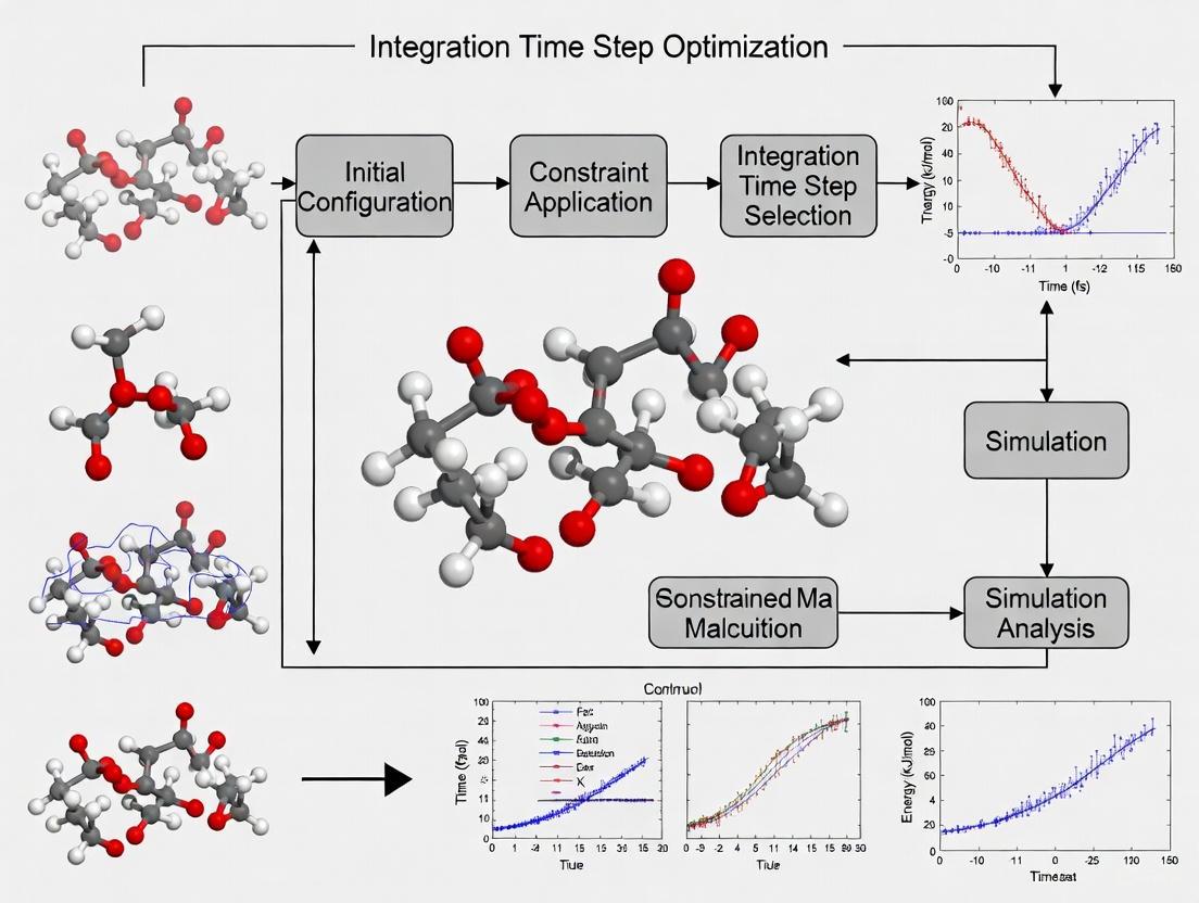
The workflow for this diagnostic process is summarized below.

Problem 2: Choosing the Right Integration and Constraint Method

The choice of integrator and constraint algorithm is crucial for achieving a stable simulation with an efficient time step.

Solution: Select algorithms based on your system's composition and the desired time step. The following table outlines the standard options available in popular software like GROMACS.

Table 2: Integration and constraint methods for enabling larger time steps [4] [2].

Method	GROMACS mdp Parameter	Typical Max Time Step	Explanation & Best For
Leap-Frog	integrator = md	1-2 fs	Default, efficient. Good for standard biomolecular simulations.
Velocity Verlet	integrator = md-vv	1-2 fs	More accurate velocities. Recommended for Nose-Hoover thermostats.
Bond Constraints (H-bonds)	constraints = h-bondsconstraint-algorithm = LINCS	2 fs	Freezes C-H/O-H/etc. bond lengths. The most common performance boost.
HMR + Constraints	constraints = h-bondsmass-repartition-factor = 3	4 fs	Mass repartitioning allows heavier H-atoms, slowing vibrations.
All-Bond Constraints	constraints = all-bonds	~4 fs	Freezes all bond lengths. Use with caution as it can restrict chemistry.

Configuration Guide:

For a typical protein-ligand system in water, aiming for a 4 fs time step using HMR, a GROMACS .mdp file should include:

The Scientist's Toolkit: Research Reagent Solutions

Table 3: Essential software and methodological "reagents" for time-step optimization experiments.

Item	Function / Role in Research	Example / Source
Velocity Verlet Integrator	A time-reversible, energy-conserving algorithm for numerically solving equations of motion. The gold standard for production MD [2].	integrator = md-vv in GROMACS [4].
LINCS Algorithm	A fast, parallelizable algorithm for constraining bond lengths. Allows a 2 fs time step by freezing bonds to hydrogen [2].	constraint-algorithm = LINCS in GROMACS [2].
Hydrogen Mass Repartitioning (HMR)	A numerical technique that scales atomic masses to slow the fastest vibrations, enabling a 4 fs time step [3].	mass-repartition-factor = 3 in GROMACS [4].
NVE (Microcanonical) Ensemble	The ensemble for testing energy conservation. The lack of a thermostat allows direct measurement of energy drift caused by the integrator [1].	pcoupl = no in GROMACS.
Multi-Time-Step (RESPA)	An integration scheme that evaluates different force components at different frequencies. Can be combined with NNPs for major speedups [6].	Implemented in Tinker-HP & FeNNol [6].
Structure-Preserving ML Integrator	An emerging machine-learning method that learns a symplectic (energy-conserving) map for long-time-step propagation [5].	Action-derived integrator [5].

Frequently Asked Questions (FAQs)

Q1: What is the fundamental theory linking Nyquist's Theorem to MD time step selection?

The Nyquist-Shannon sampling theorem establishes that to accurately represent a continuous signal without distortion (aliasing), the sampling frequency must be at least twice the highest frequency present in the signal [8] [9]. In Molecular Dynamics, this principle is directly applied to the selection of the integration time step: the time step must be small enough to sample the fastest vibrational motions in the system. The "2 fs rule" is a practical embodiment of this theorem for systems with constraints on hydrogen atoms, ensuring that the period of the fastest remaining vibration is sampled at least twice per cycle [1].

Q2: My simulation energy is unstable, even with a 2 fs time step. What should I check?

First, verify that your time step is appropriate for your specific system. A constant energy (NVE) simulation is the best test; a noticeable drift in the total energy indicates the time step may be too large or the integrator is not behaving time-reversibly [1]. Furthermore, ensure you are using a symplectic integrator (like Velocity Verlet or leap-frog), which preserves the geometric properties of Hamiltonian flow and ensures long-time near-conservation of energy [5]. For publishable results, the long-term drift in the conserved quantity should ideally be less than 1 meV/atom/ps [1].

Q3: Are there methods to safely use a time step larger than 2 fs?

Yes, several techniques can enable a larger time step by effectively reducing the system's highest frequency (Nyquist frequency):

• Constraint Algorithms: Algorithms like SHAKE or LINCS freeze the fastest bonds, particularly those involving hydrogen, removing their high frequencies from the dynamics and allowing a larger time step [1] [4].
• Hydrogen Mass Repartitioning (HMR): This technique scales the masses of the lightest atoms (like hydrogen) and adjusts the mass of the bound heavy atom to maintain total mass. With constraints, a repartitioning factor of 3 can often enable a 4 fs time step [4].
• Multiple Time-Stepping (MTS): This advanced method evaluates computationally expensive long-range forces less frequently than cheap, short-range forces, improving efficiency without sacrificing accuracy for the fast motions [4].

Q4: How does the choice of integrator influence time step selection?

The integration algorithm is crucial. Symplectic and time-reversible integrators (e.g., Velocity Verlet) have a conserved "shadow Hamiltonian" that ensures excellent long-term energy conservation, making them robust even at their stability limit. Non-symplectic integrators lack this property and typically require a much smaller time step to achieve stability [5]. The GROMACS manual recommends the md (leap-frog) integrator as being accurate enough for most production simulations [4].

Troubleshooting Guides

Problem: Unphysical Energy Increase or Simulation "Blow-Up"

This occurs when the time step is too large to accurately integrate the forces, particularly those from the highest frequency vibrations.

Diagnosis and Resolution:

• Immediate Action: Reduce the time step by 50% (e.g., from 2 fs to 1 fs) and test again.
• Verify with NVE: Run a short simulation in the NVE (constant energy) ensemble and monitor the total energy. Significant drift indicates an unstable time step [1].
• Check System Composition: Systems with very light atoms (e.g., hydrogen) have inherently higher frequency vibrations. For accurate hydrogen dynamics, time steps as low as 0.25 fs may be necessary [1].
• Inspect Constraints: If you are using constraint algorithms, ensure they are applied correctly (e.g., to all hydrogen-heavy atom bonds) and that the algorithm (e.g., SHAKE, LINCS) is not reporting failures.

Problem: SHAKE or LINCS Warning Errors

These errors indicate that the constraint solver failed to converge to a solution that satisfies the bond constraints within the allowed iterations.

Diagnosis and Resolution:

• Primary Cause: An excessively large time step is the most common cause.
• Reduce Time Step: Lower the time step until the warnings disappear.
• Increase Iterations: You can try increasing the maximum number of iterations for the constraint solver in your MD engine's parameters.
• Check Topology: Inspect your molecular topology for any incorrectly defined bonds or angles.

Problem: Poor Energy Conservation in NVE Simulation

A slight energy drift is expected in any numerical simulation, but a large drift signifies a problem.

Diagnosis and Resolution:

• Quantify the Drift: Calculate the energy drift over time. A reasonable rule of thumb is that the drift should be less than 1 meV/atom/ps for publishable results [1].
• Use a Symplectic Integrator: Ensure you are using a symplectic integrator like md or md-vv in GROMACS [4].
• Tighten Convergence Criteria: For ab initio MD, the numerical noise from poorly converged wavefunctions can cause energy drift. Tighten the electronic structure convergence criteria.
• Check for External Noise: Ensure that no other processes are introducing non-Hamiltonian forces (e.g., a poorly configured thermostat or barostat).

Experimental Protocols for Time Step Validation

Protocol 1: Empirical Validation via Energy Conservation

This is the most direct method to test if a time step is appropriate for your system and settings.

Objective: To determine the maximum time step that provides acceptable energy conservation. Materials: A well-equilibrated starting structure and topology for your system.

Method:

• Setup: Prepare multiple simulation input files, identical in every aspect except for the integration time step (dt). Test a range (e.g., 0.5, 1.0, 2.0, 2.5, 3.0, 4.0 fs).
• Run: Execute each simulation in the NVE (microcanonical) ensemble for a fixed number of steps (e.g., 10,000-50,000 steps).
• Monitor: Record the total energy throughout the simulation.
• Analyze: Plot the total energy over time for each time step.
  1. Calculate the linear drift of the total energy.
  2. A stable, non-drifting energy indicates a good time step.
  3. Identify the largest time step where the energy drift is below your required threshold (e.g., < 1 meV/atom/ps).

Protocol 2: Validation via Time-Reversibility

A key property of a good integrator is time-reversibility. This protocol tests it.

Objective: To verify the numerical reversibility of the integration scheme with the chosen time step. Materials: A well-equilibrated starting structure.

Method:

• Forward Run: Run an NVE simulation for a short period (e.g., 100-200 fs), saving the final coordinates and velocities.
• Reverse Run: Use the final state from the forward run (inverting all velocities) as the starting point for a new simulation. Run for the same simulated time.
• Compare: The final state of the reverse run should be identical to the initial state of the forward run (with velocities reversed). Any significant discrepancy indicates that the time step is too large for the integrator to behave reversibly, a sign of poor stability [1].

The following table consolidates critical numerical values and recommendations for time step selection.

Table 1: Time Step Selection Guidelines for Different Simulation Types

System / Condition	Recommended Time Step	Key Rationale	Key Reference / Test
Fully flexible (no constraints)	≤ 0.5 fs	Must sample C-H stretch (~11 fs period) at >2 points.	[1]
Bonds to H constrained (Standard)	2 fs	Removes highest frequencies; a robust community standard.	[1] [4]
With HMR & constraints	4 fs	Increased hydrogen mass lowers the highest vibrational frequency.	[4]
All-atom, general use	1 - 2 fs	Balance between accuracy and computational cost.	[1] [4]
Acceptable NVE Energy Drift	< 1 meV/atom/ps	Threshold for publishable quality results.	[1]

The Scientist's Toolkit: Essential Materials and Software

Table 2: Key Research Reagents and Software Solutions

Item / Software	Function in Time Step Optimization
Constraint Algorithms (SHAKE, LINCS)	"Freeze" the fastest bond vibrations (e.g., C-H), allowing a larger time step by effectively raising the Nyquist frequency.	[1] [4]
Symplectic Integrator (Velocity Verlet, Leap-Frog)	A class of numerical solvers that preserve the geometric structure of Hamiltonian mechanics, ensuring excellent long-term energy conservation.	[4] [5]
Hydrogen Mass Repartitioning (HMR)	A technique that scales atomic masses to slow down the highest frequency motions, enabling a larger integration time step.	[4]
Multiple Time-Stepping (MTS)	An efficiency method where computationally expensive long-range forces are calculated less frequently than cheap, short-range forces.	[4]
NVE (Microcanonical) Ensemble	The primary simulation ensemble used for testing and validating the stability and energy conservation of a chosen time step.	[1]

Workflow and Relationship Visualizations

The following diagram illustrates the logical workflow for selecting and validating an integration time step in an MD simulation.

Time Step Selection and Validation Workflow

Frequently Asked Questions

Q1: What is the fundamental purpose of using a constraint algorithm in molecular dynamics?

Constraint algorithms are methods used to satisfy Newtonian motion for rigid bodies consisting of mass points. In molecular dynamics simulations, they are applied to maintain specific degrees of freedom, most commonly bond lengths and angles, at fixed values. This is achieved by introducing constraint forces, often solved via Lagrange multipliers, which act to keep atomic distances constant without affecting the system's dynamics and energetics. This allows for computational efficiency by neglecting fast vibrations, enabling the use of larger integration time steps [10].

Q2: My simulation with SHAKE fails to converge, reporting that the "deviation is too large." What are the primary causes and solutions?

The SHAKE algorithm is iterative and will report an error if it cannot reset coordinates because the deviation is too large or if a maximum number of iterations is surpassed [11]. Primary causes and solutions are:

• Cause: An excessively large integration time step, leading to overly large atomic displacements in the unconstrained update.
  • Solution: Reduce the simulation time step. For bonds with hydrogen atoms, a time step of 1-2 fs is common when constraints are applied [2].
• Cause: Incorrect or inconsistent parameters in the molecular topology (e.g., incorrect constraint distances).
  • Solution: Carefully check your system's topology file to ensure all constraint parameters are correctly defined.
• Cause: System instability, perhaps due to steric clashes or incorrect initial configuration.
  • Solution: Conduct a thorough energy minimization before starting the dynamics and ensure your starting structure is physically realistic.

Q3: When should I use SETTLE instead of SHAKE or LINCS?

The SETTLE algorithm should be used for the specific case of rigid water molecules [11]. It is an analytical solution, meaning it is non-iterative and finds the correct constrained coordinates in a single, fast calculation. Since water molecules often constitute over 80% of a simulation system, using SETTLE for them provides significant performance gains and reduces rounding errors compared to using an iterative solver like SHAKE [11] [2].

Q4: Can LINCS be used to constrain both bonds and angles in any molecule?

No, LINCS should not be used with coupled angle constraints [11]. While it is excellent for bond constraints and isolated angle constraints, its mathematical formulation involves inverting a matrix whose eigenvalues can become larger than one in molecules with high connectivity, such as those created when constraining angles with additional distance constraints. This can lead to instability and convergence issues. For constraining both bonds and angles, SHAKE is a more suitable algorithm [2].

Q5: How do I choose between the Velocity Verlet and Leap-Frog integrators when using constraints?

The Velocity Verlet and Leap-Frog integrators are mathematically equivalent and produce identical trajectories [2]. The primary difference is practical:

• Velocity Verlet calculates positions, velocities, and forces at the same point in time.
• Leap-Frog calculates velocities staggered by half a time step relative to positions and forces. The key consideration is for simulation restarts. Changing the integrator mid-simulation will introduce a discontinuity because the saved velocities in the restart files are defined at different times [2]. You should choose one integrator and maintain it for the entire simulation.

Troubleshooting Guides

Issue: Energy Drift in Constrained Simulation

Problem Description The total energy of the system shows a consistent upward or downward drift over time, indicating a lack of energy conservation.

Diagnosis Steps

• Check Constraint Tolerance: A tolerance that is too loose can lead to small violations of constraints, causing energy drift. Monitor the reported constraint deviation in your simulation log file.
• Verify Time Step: Even with constraints, an overly large time step for the remaining degrees of freedom can cause instability.
• Identify Algorithm-Specific Issues:
  • For SHAKE: Ensure the number of iterations (SHAKEMAXITER or equivalent) is sufficient to achieve convergence for all constraints [12].
  • For LINCS: In single precision, simulations with normal constraints can show a quadratic energy drift for systems larger than 100-200 nm. SETTLE, in contrast, has a linear dependence, making it more accurate for large systems in single precision [11].
• Inspect for Hardware/Algorithm Mismatch: When using GPU acceleration, ensure all parts of the computation (including constraints) are executed on the GPU to minimize costly CPU-GPU communication, which can introduce errors [13].

Resolution Actions

• Tighten the constraint tolerance (e.g., SHAKETOL in VASP [12]) and increase the maximum number of iterations.
• Reduce the integration time step.
• Consider using the lincs-order parameter in GROMACS to increase the expansion order for the matrix inversion, improving accuracy [11].

Issue: Performance Degradation with LINCS on a GPU

Problem Description The simulation runs slower than expected when using the LINCS constraint algorithm on GPU-accelerated hardware.

Diagnosis Steps

• Profile the Simulation: Use profiling tools provided with your MD software (e.g., gmx mdrun -verbose) to identify if the constraint calculation is a bottleneck.
• Check for Parallelization Settings: Verify that the parallel version of LINCS (P-LINCS) is enabled for simulations running on multiple domains.
• Review System Connectivity: As per the LINCS formulation, the inversion of the constraint coupling matrix consumes significant CPU time. Molecules with high connectivity (like rings) make this matrix less sparse, increasing computation time [11].

Resolution Actions

• Ensure you are using a recent version of your MD software with optimized GPU kernels for constraints.
• For large systems, confirm P-LINCS is active. In GROMACS, this is automatic when running in parallel [11].
• For small to medium-sized systems, the performance may be limited by the overhead of CPU-GPU communication. A hybrid approach where the CPU handles some tasks may be more efficient [14].

Comparative Data on Constraint Algorithms

The table below summarizes the core characteristics of the primary constraint algorithms.

Table 1: Key Characteristics of SHAKE, LINCS, and SETTLE Algorithms

Feature	SHAKE	LINCS	SETTLE
Core Methodology	Iterative Lagrange multiplier solver [10]	Non-iterative, matrix-based projection [11]	Analytical, non-iterative solution [11]
Typical Relative Tolerance	User-defined (e.g., SHAKETOL) [12]	Fixed (deviation < 0.0001 per constraint) [11]	Exact by design [11]
Supported Constraints	Bonds and angles [2]	Bonds and isolated angles [11]	Only rigid water geometries [11]
Parallel Efficiency	Low, difficult to parallelize [2]	High, with P-LINCS for parallel runs [11]	High for water molecules [11]
Performance & Stability	Stable, slower (iterative), good for complex constraints [2]	Faster than SHAKE, stable for bonds, unstable for coupled angles [11] [2]	Very fast and accurate for rigid water [11]

Experimental Protocols

Protocol 1: Implementing Bond Constraints using SHAKE in a VASP MD Simulation

This protocol details the steps to perform a constrained molecular dynamics simulation using the SHAKE algorithm in VASP [12].

• Define Geometric Constraints: Create an ICONST file. To constrain a bond between atoms 1 and 2 to a distance of 1.0 Å, include the line: R 1 2 1.0. Set the STATUS parameter for this coordinate to 0.
• Set MD Parameters: In the INCAR file, configure the following parameters:
  • IBRION = 0 (MD run)
  • TEBEG (Starting temperature)
  • POTIM (Integration time step)
  • NSW (Number of MD steps)
• Select Thermostat: Choose and configure a thermostat by setting:
  • MDALGO = 1 (Andersen thermostat) and ANDERSEN_PROB, OR
  • MDALGO = 2 (Nose-Hoover thermostat) and SMASS
• Configure SHAKE: Set the convergence parameters for the SHAKE algorithm:
  • SHAKETOL: The relative tolerance for satisfying constraints.
  • SHAKEMAXITER: The maximum number of iterations for the SHAKE procedure.
• Execute the Simulation: Run VASP with the standard command (vasp_std). Monitor the OUTCAR file for messages regarding constraint convergence.

Protocol 2: Configuring Constraints for Increased Time Step in GROMACS

This protocol allows for doubling the simulation time step from 1 fs to 2 fs by constraining bonds involving hydrogen atoms [2].

• Prepare the System Topology: Ensure your topology file (e.g., .top) correctly defines all molecular bonds.
• Configure the MDP Parameters: In your GROMACS run parameter file (.mdp), set the following key lines:
  • integrator = md (or md-vv for Velocity Verlet)
  • dt = 0.002 ; Time step of 2 fs
  • constraints = h-bonds ; Constrain all bonds involving hydrogen atoms
  • constraint-algorithm = LINCS ; Use the LINCS algorithm (default)
• Set LINCS Parameters (Optional): For higher accuracy, especially in energy minimization, you can adjust:
  • lincs-order = 4 ; Order of the matrix expansion
  • lincs-iter = 1 ; Number of iterations (1 is standard for MD)
• Run the Simulation: Process the topology with gmx grompp and execute with gmx mdrun.

Workflow Visualization

The following diagram illustrates the logical decision process for selecting an appropriate constraint algorithm in a molecular dynamics simulation.

Algorithm Selection Workflow

The Scientist's Toolkit: Essential Research Reagents & Materials

Table 2: Key Software and Hardware Solutions for Constrained MD Simulations

Item Name	Function / Relevance
GROMACS	A high-performance MD software package that implements SHAKE, LINCS, and SETTLE algorithms. It is highly optimized for both CPU and GPU execution [11] [2].
VASP	A plane-wave DFT code that implements constrained MD using the SHAKE algorithm for ab initio simulations [12].
OpenMM	A MD toolkit designed for high performance on GPUs. It handles constraints and all force calculations directly on the GPU, minimizing communication overhead [14].
LAMMPS	A classical, general-purpose MD code with GPU support via OpenCL or CUDA. It uses a hybrid approach where the GPU calculates non-bonded forces while the CPU handles constraints and bonded forces [14].
NVIDIA/AMD GPUs	Graphics Processing Units that provide massive parallelism, significantly accelerating the calculation of forces and constraint solvers in MD simulations [13] [14].
Cerebras WSE	A wafer-scale engine that offers unprecedented simulation rates for large-scale MD, enabling millisecond-scale simulations by overcoming traditional hardware constraints [15].

Frequently Asked Questions

FAQ 1: Why is a short time step (e.g., 1-2 fs) mandatory in molecular dynamics simulations? The time step is fundamentally limited by the highest frequency vibration in the system, typically involving hydrogen atoms (e.g., C-H bonds vibrating at ~3000 cm⁻¹, with a period of about 11 femtoseconds) [1]. According to the Nyquist theorem, to accurately capture a motion, you must sample it at least twice per period [1]. Therefore, a time step of 2 fs or less is required to numerically integrate these fastest motions without the simulation becoming unstable and "blowing up" [1].

FAQ 2: What are the immediate, observable consequences of an excessively large time step? Using a time step that is too large leads to a rapid and unphysical drift in the system's conserved quantity (e.g., total energy in NVE simulations) [1]. This indicates that the integrator is no longer time-reversible and is failing to accurately solve the equations of motion. In severe cases, this results in a catastrophic simulation failure where the energy "blows up" [1].

FAQ 3: Can't we just use constraints or mass repartitioning to gain a larger time step? While techniques like SHAKE (for bonds) and Hydrogen Mass Repartitioning (HMR) allow for larger time steps (e.g., 4 fs) by removing or slowing the highest frequency motions, they are not a free pass [16] [17]. HMR, for instance, can alter the dynamics of the system. Research has shown it can retard processes like protein-ligand recognition by affecting ligand diffusion and intermediate stability, potentially negating the computational performance gains for studying kinetic processes [17] [18]. These methods require careful validation for your specific research objective.

FAQ 4: My simulation uses the NVT ensemble. What is the "conserved quantity" I should monitor? In ensembles other than NVE, the total energy is not constant. For NVT simulations using a method like Nosé-Hoover, the conserved quantity includes extra terms from the thermostat [1]. Your MD software manual will specify the exact conserved quantity for the chosen integrator and ensemble. A drift in this quantity indicates inaccuracies in your time step or integration method.

FAQ 5: What does the "flying ice-cube" effect refer to? This is a phenomenon sometimes observed in dynamics simulations using certain thermostats (e.g., Nosé-Hoover), where thermal energy is progressively bled from the internal conformational degrees of freedom into the overall translational and rotational (global) degrees of freedom [16]. This results in an unphysical, "freezing" of the molecule's internal motion while the entire molecule drifts or rotates with increasing speed, resembling a flying ice cube.

---

Troubleshooting Guides

Problem 1: Energy Drift in NVE Simulations

Observed Symptom: The total energy of the system shows a consistent upward or downward drift over time, instead of fluctuating around a stable average.

Diagnostic Methodology: This diagnostic experiment is the most direct way to assess the stability of your integrator and the suitability of your time step [1].

• 1. Configure the Simulation: Set up a short simulation in the NVE (microcanonical) ensemble. This isolates the integrator's performance from the effects of a thermostat or barostat.
• 2. Run and Monitor: Run the simulation and carefully monitor the total energy.
• 3. Analyze the Drift: Calculate the long-term drift in the total energy. A reasonable rule of thumb is that the drift should be less than 1 meV/atom/ps for publishable results, though up to 10 meV/atom/ps may be acceptable for qualitative work [1].

Solution Actions:

• Primary Action: Reduce the time step. If you observe a significant drift, reduce your time step by 25-50% (e.g., from 2 fs to 1.5 fs) and repeat the NVE test.
• Verify Rigidity: Ensure that constraints on bonds involving hydrogen (e.g., via SHAKE, LINCS, or SETTLE for water) are correctly applied [17].
• Check Symplectic Nature: Confirm you are using a symplectic (time-reversible) integrator like Velocity Verlet or Leap-Frog, which are designed for long-term energy conservation [1].

The diagnostic workflow for this problem is summarized below:

Problem 2: Flying Ice-Cube Effect

Observed Symptom: The internal structure of your protein or molecule appears to become rigid and "frozen" over time, while the entire molecule exhibits unnaturally large translational or rotational motion.

Diagnostic Methodology: Monitor the kinetic energy associated with different degrees of freedom separately over the course of an NVT simulation.

• 1. Decompose Kinetic Energy: Use analysis tools to track the kinetic energy of the system's center-of-mass translation, rotation, and internal vibrations separately.
• 2. Identify Imbalance: The "flying ice-cube" effect is confirmed if you see a continuous increase in the global (center-of-mass and rotational) kinetic energy with a corresponding decrease in the internal kinetic energy [16].

Solution Actions:

• Apply Momentum Removal: Most MD software includes an option to periodically remove the center-of-mass momentum (and angular momentum) during the simulation. In GROMACS, this is controlled by the comm-mode and nstcomm parameters [19]. Apply this every 10-100 steps.
• Alternative Thermostat: Consider switching to a stochastic thermostat (e.g., Langevin dynamics) or a different deterministic thermostat that does not exhibit this effect as strongly.

Problem 3: Constraint Failure (e.g., SHAKE/LINCS Warnings)

Observed Symptom: The simulation crashes with warnings about the failure of the constraint algorithm (e.g., "SHAKE failure," "LINCS warnings") indicating that bond lengths could not be maintained.

Diagnostic Methodology: This is often a direct consequence of a time step that is too large for the remaining degrees of freedom after constraints are applied [17].

• 1. Check Time Step Value: For all-atom simulations with bonds to hydrogen constrained, the maximum stable time step is typically 2 fs. If you are using a value larger than this, it is the primary suspect.
• 2. Inspect System: Look for parts of the system with particularly stiff degrees of freedom that may not be fully handled by the constraint algorithm.

Solution Actions:

• Reduce Time Step: Immediately reduce the time step to 2 fs or lower.
• Consider Advanced Methods: For a performance boost, instead of arbitrarily increasing the time step, investigate methods like Hydrogen Mass Repartitioning (HMR) which scales the mass of hydrogen atoms to allow for a 4 fs time step while keeping the total molecular mass constant [17] [19]. Always validate that this method does not impact the dynamics you wish to study [17].

---

Quantitative Guidelines for Time Step Selection

The table below summarizes key metrics and reference values for choosing and validating your integration time step.

Parameter	Typical Value / Rule	Purpose & Rationale
Time Step (Δt)	0.5 - 2.0 fs	Default range for all-atom, constrained MD. Balances stability and computational cost [1].
Nyquist Criterion	Δt ≤ (Period of Fastest Vibration) / 2	The absolute maximum time step; often a smaller fraction (e.g., 0.01-0.033 of the period) is used for accuracy [1].
HMR Time Step	4 fs	Allows a larger time step by repartitioning mass to slow high-frequency vibrations [17] [19].
Acceptable Energy Drift (NVE)	< 1 meV/atom/ps	Target for accurate, publishable simulations [1].
MTS Factor (if applicable)	2 - 4	Interval for evaluating slow forces (e.g., long-range electrostatics) in multiple-time-stepping schemes [19].

---

The Scientist's Toolkit: Essential Research Reagents & Solutions

This table lists key computational "reagents" and methods essential for conducting robust constrained MD simulations.

Item / Method	Function in Research
SHAKE / LINCS / SETTLE	Algorithms that impose holonomic constraints on bond lengths and angles, allowing for a larger time step by removing the highest frequency vibrations [16] [17].
Velocity Verlet Integrator	A symplectic (time-reversible) integrator that ensures long-term stability and energy conservation, making it the gold standard for MD [1].
Hydrogen Mass Repartitioning (HMR)	A mass-scaling technique that allows for a ~2x larger time step by repartitioning mass from heavy atoms to bonded hydrogens, conserving total molecular mass [17] [19].
Nosé-Hoover Thermostat	A deterministic algorithm for maintaining constant temperature (NVT ensemble). Can sometimes exhibit the "flying ice-cube" effect, requiring corrective measures [16].
Langevin Dynamics	A stochastic thermostat that adds friction and noise, effectively controlling temperature and helping to prevent the "flying ice-cube" effect [19].

---

Relationship Between Time Step and System Dynamics

The following diagram illustrates the core logic governing the choice of time step and the advanced methods used to modify it, based on the Nyquist theorem and system properties.

Frequently Asked Questions (FAQs)

1. What is the fundamental trade-off between computational speed and physical accuracy in MD simulations? The trade-off originates from the need to use discrete time steps to numerically integrate the equations of motion. A larger time step (e.g., 2 femtoseconds) increases simulation speed but risks instability and physical inaccuracies, as it may not properly capture high-frequency molecular vibrations like bond stretches. A smaller time step (e.g., 0.5 femtoseconds) improves accuracy but drastically increases computational cost, as more steps are required to simulate the same physical time [20] [21].

2. How do constraint algorithms like LINCS and SHAKE help manage this trade-off? Constraint algorithms allow for larger integration time steps without sacrificing the stability of the simulation. They do this by mathematically fixing the lengths of the fastest vibrating bonds (e.g., C-H bonds), which would otherwise require a very small time step to resolve. LINCS is generally faster and more stable than SHAKE, but SHAKE may be more suitable for complex constraint networks involving angles [11].

3. What is the Multiple Time-Stepping (MTS) method, and how does it improve efficiency? The reversible Reference System Propagator Algorithm (r-RESPA) is an MTS method that calculates different types of forces at different frequencies. Computationally expensive forces, such as long-range or complex three-body interactions, are calculated less frequently (e.g., every 4 steps), while fast, short-range forces are calculated at every step. This can significantly reduce computational cost while preserving accuracy [20].

4. My simulation is unstable or "blows up." Could the time step be the issue? Yes, an excessively large time step is a common cause of instability. The first step is to reduce the time step, often to 1 femtosecond or less, to see if stability is restored. Secondly, ensure that a constraint algorithm is being applied correctly to all relevant bonds. Finally, verify that the selected thermostat and barostat coupling constants are appropriate for your chosen time step [11] [21].

5. How does the choice of hardware influence the speed-accuracy balance? Advances in hardware, such as Graphics Processing Units (GPUs) and specialized architectures like the Cerebras Wafer Scale Engine, can dramatically increase simulation speed, allowing you to simulate more atoms or longer timescales without compromising on time step size or physical models. This can shift the trade-off, making previously intractable simulations feasible [15].

6. What are the key metrics to monitor when optimizing a simulation? To ensure a good balance, monitor the conservation of total energy in your system (NVE ensemble), the temperature and pressure stability (NVT, NPT ensembles), and the relative constraint deviation (should be less than 0.0001). It is also good practice to compare simulated structural properties, like radial distribution functions, against known experimental or theoretical data [11] [21].

---

Quantitative Data for Common Simulation Parameters

The following table summarizes key parameters and their typical values, providing a starting point for configuring your simulations.

Table 1: Common Parameters for Constrained MD Simulations

Parameter	Recommended Range	Description & Impact
Integration Time Step (TimeStep)	1 - 2 fs	The core parameter controlling simulation speed and stability. Larger values speed up calculations but risk inaccuracies [21].
Constraint Tolerance (SHAKE)	0.0001	The relative tolerance for satisfying constraints. A stricter tolerance improves accuracy at a higher computational cost [11].
LINCS Order	4 - 12	The order of the matrix expansion in LINCS. A higher order improves the accuracy of constraint satisfaction [11].
MTS Factor (for r-RESPA)	2 - 4	The ratio of the long time step to the short time step. A higher factor reduces cost but may miss some slower force components [20].
Thermostat Coupling Constant (Tau)	0.1 - 1.0 ps	The time constant for temperature coupling. A smaller value tightly controls temperature but may affect dynamics [21].

---

Experimental Protocols

Protocol 1: Implementing Multiple Time-Stepping with r-RESPA

This protocol outlines how to set up an r-RESPA simulation to reduce the computational cost of expensive force calculations, such as three-body interactions.

• Force Splitting: Separate the total force acting on particles into distinct categories based on their computational cost and frequency. Typically, this is a "fast" force (e.g., short-range bonded and non-bonded interactions) and a "slow" force (e.g., long-range electrostatics or three-body potentials) [20].
• Time Step Definition: Define two time steps:
  • Short Time Step (dt_fast): Used to integrate the "fast" forces. This is your base time step, typically 1 fs.
  • Long Time Step (dt_slow): Used to integrate the "slow" forces. This is a multiple of the short time step, e.g., dt_slow = 4 * dt_fast [20].
• Integration Loop: In the simulation code, structure the time integration loop as follows:
  • At every short time step, calculate and integrate the "fast" forces.
  • Only at every long time step (e.g., every 4th step), calculate and integrate the "slow" forces.
• Validation: Run a short simulation with r-RESPA and compare system properties (e.g., potential energy, temperature, pressure) against a reference simulation using a single, small time step to ensure accuracy has not been compromised.

The workflow for this protocol is summarized in the following diagram:

Protocol 2: Applying Bond Constraints with the LINCS Algorithm

This protocol details the steps for using the LINCS algorithm to constrain bond lengths, allowing for a larger integration time step.

• Identify Constrained Bonds: Select which bonds to constrain. Typically, all bonds involving hydrogen atoms are constrained because of their high vibration frequency [11].
• Algorithm Configuration: In your MD software, select the LINCS algorithm. Set the lincs_order parameter (e.g., 6) which determines the accuracy of the constraint application. Set the lincs_iter parameter, defining the number of iterations to correct for rotational lengthening [11].
• Unconstrained Coordinate Update: Perform a normal, unconstrained update of particle coordinates based on the current velocities and forces, using the desired larger time step (e.g., 2 fs).
• LINCS Projection (Step 1): Apply the first LINCS projection to the new coordinates. This step sets the projection of the new bonds onto the old bond directions to zero, but does not yet set the correct bond lengths [11].
• LINCS Correction (Step 2): Apply a correction for the lengthening of bonds due to rotational motion. This step is often iterative, but in production MD, usually only one iteration is applied per time step [11].
• Verification: Monitor the Relative Constraint Deviation in the simulation log file. This value should remain very small (e.g., < 0.0001) for all constrained bonds throughout the simulation [11].

Table 2: Troubleshooting Common MD Simulation Issues

Problem	Possible Cause	Solution
Energy Drift	Time step too large; Constraints not satisfied.	Reduce the time step; Check constraint tolerance and algorithm.
LINCS Warning	A bond is rotating too much in one step.	Reduce the time step; Increase the LINCS order (lincs_order).
Pressure/Temperature Instability	Incorrect thermostat/barostat settings.	Adjust the coupling constants (Tau); Ensure mass and time scales are compatible.
Poor Performance	Calculating expensive forces too often.	Implement the r-RESPA method to calculate slow forces less frequently [20].

---

The Scientist's Toolkit: Essential Research Reagents & Solutions

Table 3: Key Software and Algorithms for Constrained MD

Item	Function in Research
LINCS Algorithm	A constraint algorithm used to reset bond lengths to their correct values after an unconstrained update, allowing for larger time steps. It is generally faster and more stable than SHAKE [11].
SHAKE Algorithm	An iterative algorithm that solves for Lagrange multipliers to satisfy distance constraints. It is a foundational method for enabling stable simulations with larger time steps [11].
r-RESPA (MTS)	A multiple time-stepping algorithm that improves computational efficiency by evaluating computationally inexpensive forces more frequently than expensive ones [20].
Velocity Verlet Integrator	The core numerical integration algorithm used in many MD packages to update particle positions and velocities at each time step [21].
Thermostat (e.g., Nose-Hoover)	A method to control the simulation temperature, mimicking a thermal bath. Essential for simulating NVT (canonical) ensembles [21].

Practical Protocols: Implementing Constraints and Selecting Time Steps for Biomolecular Systems

Frequently Asked Questions (FAQs)

1. Which integrator should I use as a default for new constrained dynamics simulations? For most new simulations, the Velocity Verlet integrator is recommended. It calculates positions and velocities synchronously at the same time point, making it more straightforward to initiate and analyze simulations. Its formulation is algebraically equivalent to the leap-frog algorithm, producing identical trajectories, but it provides synchronous velocity and position data which is often more convenient for analysis and calculating observables like kinetic energy [22] [2].

2. I am getting discontinuous kinetic energy when I restart my simulation. Could the integrator be the cause? Yes. This is a known issue when switching between leap-frog and Velocity Verlet integrators, or when using leap-frog restart files. The leap-frog algorithm stores velocities shifted by half a time-step compared to positions. When you restart a simulation with a different integrator, this phase difference introduces an instantaneous change in the computed kinetic energy [2]. To ensure seamless restarts, maintain the same integrator used to generate the initial simulation data.

3. Are Velocity Verlet and leap-frog equally accurate and stable for simulations with bond constraints? Yes, both methods are mathematically equivalent and generate identical trajectories [2]. They are both time-reversible and energy-conserving (symplectic), which makes them superior to simpler methods like Euler integration for molecular dynamics [22] [2]. The choice between them does not affect the numerical stability or accuracy of the constrained dynamics.

4. How does the choice of constraint algorithm (like SHAKE or LINCS) interact with the integrator? The constraint algorithm operates alongside the integrator. While the integrator (Velocity Verlet or leap-frog) updates the atomic positions and velocities, the constraint algorithm (e.g., SHAKE, LINCS, or SETTLE) corrects these positions to satisfy bond-length constraints. The performance gain from a faster constraint algorithm like LINCS, which can be 3-4 times faster and more accurate than SHAKE in parallel simulations, is independent of the integrator choice [23].

5. In the GROMACS manual, the leap-frog is listed as md and Velocity Verlet as md-vv. Which one is more efficient? In practice, both have comparable computational cost per time-step [22] [24]. GROMACS documentation notes that the md-vv-avek (Velocity Verlet) variant can be more accurate for kinetic energy calculations, as it computes the kinetic energy as the average of the two half-step kinetic energies [2]. For most simulations, the performance difference is negligible, and the choice should be based on convenience for data handling and analysis.

Troubleshooting Guides

Problem: Unphysical Energy Drift in Constrained Simulation

Symptoms A steady increase or decrease in total energy over time in an NVE (microcanonical) simulation.

Possible Causes and Solutions

Cause	Diagnostic Steps	Solution
Time step is too large	Check log files for warnings; monitor bond length variations.	Reduce time step to 1-2 fs for unconstrained H-bonds, or to 4 fs when using H-mass repartitioning [2].
Insufficient pair-list buffer	Check energy drift report in GROMACS log; it is likely small but non-zero.	Allow GROMACS to auto-determine the Verlet buffer size; it adjusts the pair-list cut-off to account for atomic diffusion [24].
Constraint algorithm failure	Check for convergence warnings in log files from SHAKE or LINCS.	For polymers, consider using modern algorithms like ILVES-PC, which uses Newton's method for more accurate and rapid convergence of constraints [23].

Problem: Inaccurate Temperature Calculation

Symptoms The computed temperature from kinetic energy consistently deviates from the target temperature.

Possible Causes and Solutions

Cause	Diagnostic Steps	Solution
Leap-frog velocity phase	Confirm if kinetic energy is calculated from v(t) or v(t+Δt/2).	Use the md-vv-avek integrator in GROMACS for a more accurate kinetic energy calculation [2].
Flying ice cube" effect	Check if the system's center-of-mass velocity is non-zero and increasing.	Enable center-of-mass motion removal at every time step to prevent spurious kinetic energy buildup [24].

Integrator Comparison and Selection Guide

The following table summarizes the core characteristics of the Velocity Verlet and leap-frog integrators.

Table 1: Key Differences Between Velocity Verlet and Leap-Frog Integrators

Feature	Velocity Verlet	Leap-Frog
Formulation	Synchronous: r(t) & v(t) are known and updated together [2].	Staggered: r(t) and v(t±Δt/2) are known at a given time [2].
Initialization	Straightforward; requires initial positions and velocities [2].	Requires initial positions and the previous half-step velocity, which can be estimated [24].
Trajectory Output	Positions and velocities are synchronous in output files [2].	Velocities in output files are shifted by half a time-step relative to positions [2].
Kinetic Energy Calculation	Natural and accurate; velocities are known at the same time as positions. Can be even more accurate with md-vv-avek [2].	Requires approximation, as v(t) is not directly available (must be estimated from v(t±Δt/2)) [2].
Mathematical Equivalence	Yes, produces identical trajectories to leap-frog [2].	Yes, produces identical trajectories to Velocity Verlet [2].
Restart Compatibility	High; restart files are self-consistent.	Low; changing from leap-frog to Verlet upon restart causes kinetic energy discontinuity [2].

Experimental Protocols for Integrator Assessment

Protocol 1: Benchmarking Integrator Performance and Energy Conservation

This protocol assesses the practical performance and energy conservation of the chosen integrator in your specific system.

Research Reagent Solutions

Item	Function in the Protocol
Molecular Dynamics Software (e.g., GROMACS, NAMD)	Provides the computational environment and implemented integration algorithms [2] [21].
System Topology and Force Field	Defines the potential energy V and forces F for your molecular system [24].
Constraint Algorithm (e.g., LINCS, SHAKE)	Allows the use of a longer time step by constraining bond vibrations [2] [23].
Stable Protein or Polymer System	A well-equilibrated test system for benchmarking.

Methodology

• System Preparation: Use a fully equilibrated molecular system (e.g., a solvated protein or polymer in a box).
• Simulation Setup: Run multiple short simulations in NVE ensemble using:
  • Integrator: md (leap-frog) and md-vv (Velocity Verlet)
  • Constraint algorithm: LINCS (for proteins) or SETTLE (for water)
  • Time steps: 1 fs, 2 fs, and 4 fs (if using H-mass repartitioning)
• Data Collection: Monitor the total energy, temperature, and pressure over time. Record the simulation performance (ns/day).
• Analysis: Calculate the energy drift (kJ/mol/ps) and check for equipartition among degrees of freedom. Compare the performance and stability between the two integrators.

Protocol 2: Evaluating the Impact of Constraint Algorithms

This protocol tests how the choice of constraint algorithm interacts with the integrator to affect simulation accuracy and speed.

Methodology

• Baseline Simulation: Set up a simulation with a standard time step (e.g., 2 fs) using the Velocity Verlet integrator and the SHAKE algorithm.
• Algorithm Comparison: Run the same simulation with different constraint algorithms (e.g., SHAKE, LINCS, P-LINCS). For polymer systems, if available, test specialized algorithms like ILVES-PC [23].
• Accuracy Metric: Compute the RMSD of constrained bond lengths from their ideal values throughout the simulation. A lower RMSD indicates higher accuracy.
• Performance Metric: Compare the total simulation time and time spent on constraint satisfaction for each algorithm-integrator pair.

Workflow Visualization

The diagram below illustrates the logical workflow for selecting and troubleshooting an integrator in constrained MD simulations.

A technical guide for molecular dynamics researchers

What are constraint algorithms and why are they used in MD simulations?

Constraint algorithms are mathematical methods used in Molecular Dynamics to fix the lengths of specific bonds (and sometimes angles) in the simulation. Instead of allowing these bonds to vibrate, which requires a very small time step to integrate accurately, they are held rigid. This allows for a larger integration time step (e.g., 2 fs instead of 0.5 fs), significantly reducing the computational cost of the simulation without sacrificing the stability of the molecular geometry [11].

In GROMACS, the two primary constraint algorithms are LINCS (the default) and SHAKE [11]. The SETTLE algorithm is used specifically for rigid water molecules [11]. The choice of which bonds to constrain is a critical strategic decision that balances computational speed against physical accuracy.

What is the practical difference between 'all-bonds', 'h-bonds', and 'h-angles'?

The constraints directive in your GROMACS .mdp file controls which bonds in the molecular system are converted into constraints. This choice directly impacts the maximum stable integration time step you can use. The following table summarizes the common constraint levels.

Constraint Level	Bonds Constrained	Typical Use Case	Max Stable dt (fs)
all-bonds	All chemical bonds	Standard all-atom simulations	1-2
h-bonds	Bonds involving hydrogen	Most common for all-atom simulations	2
h-angles	Bonds involving hydrogen + H--X--H angles	Allows for larger time steps with mass repartitioning	3-4

• all-bonds: This setting constrains the lengths of every single chemical bond in the system. While this provides the most rigid geometry, the fastest vibrational frequencies in the system (like those in heavy-atom bonds) still dictate a relatively small time step, typically 1-2 fs.
• h-bonds: This is the most commonly used option for all-atom simulations. It constrains only bonds that involve a hydrogen atom. Since hydrogen is the lightest atom, its bonds have the highest frequency vibrations. By constraining these, the limiting frequency is removed, allowing for a time step of 2 fs, which is the standard for most simulations.
• h-angles: This more advanced option goes a step further by constraining not only bonds involving hydrogen but also angles where the hydrogen is the central atom (e.g., H--X--H angles). This level of constraint, especially when combined with mass repartitioning, can enable even larger time steps of 3-4 fs [25]. Mass repartitioning works by scaling down the masses of the lightest atoms (typically hydrogens) and subtracting that mass from the atom they are bound to, which slows down the highest frequency motions and improves stability [25].

How do I select and configure a constraint algorithm in GROMACS?

The constraint algorithm is selected in the .mdp file. LINCS is generally recommended for its speed and stability, especially with bond constraints and for Brownian dynamics [11].

.mdp File Parameters:

Algorithm Selection Guide:

• LINCS: The default and recommended algorithm. It is non-iterative and faster than SHAKE. It works well with bond constraints and isolated angle constraints but should not be used with coupled angle constraints as this can lead to large eigenvalues and instability [11].
• SHAKE: An iterative algorithm that will continue until all constraints are satisfied within a given relative tolerance. It is more general but slower [11].
• SETTLE: An analytical algorithm used specifically for rigid water models (like SPC, TIP3P, TIP4P). It is selected automatically in the molecule's topology definition via the [ settles ] directive and is highly accurate and efficient [11] [26].

I'm getting a "domain decomposition" error after adding restraints. How can I fix it?

This fatal error occurs when the Domain Decomposition (DD) algorithm, used for parallel computing, cannot split the simulation box into cells that are large enough to handle the constraint and/or bonded interactions.

Troubleshooting Steps:

• Increase the box size: A common cause is having a small simulation box with long-distance bonded restraints (e.g., type 6 restraints). Adding more solvent padding increases the box size, giving the DD algorithm more space to work with. However, this also increases the total atom count and computational cost [27].
• Adjust DD parameters: Use the -rdd or -dds command-line options with mdrun. The -rdd option can be used to increase the maximum distance for multi-body interactions. Alternatively, using -dds with a value less than 1.0 (e.g., 0.8) can force mdrun to choose a different, potentially more compatible, decomposition.
• Reduce the number of MPI ranks: The error message often specifies a number of ranks that is incompatible. Running with fewer cores can solve the problem immediately, as it results in larger domain decomposition cells. A good rule of thumb is to have at least ~100 atoms per core [27].
• Use a workaround for long restraints: If the error is triggered by long-distance bonded restraints meant to maintain tertiary structure, consider using the pull code as an alternative. By defining two pull groups and using an "umbrella" potential with the rate set to zero, you can effectively create a harmonic restraint at a fixed distance without introducing a formal bonded term that complicates domain decomposition [27].

Example pull code configuration:

My simulation crashes with a LINCS warning. What does it mean?

LINCS warnings indicate that the constraint algorithm is struggling to reset the bond lengths correctly, often due to large forces causing atoms to move excessively between steps.

Common Errors and Solutions:

• "LINCS WARNING: ... max drift ...": This indicates that one or more bonds have rotated too much in a single time step, making it difficult for LINCS to correctly project the constraints.

  • Solution: Reduce your time step (dt). A 2 fs time step is standard for constraints = h-bonds. If you are using a larger step (e.g., 3-4 fs with h-angles), try reducing it to 2 fs to see if the problem resolves.
  • Check the system setup: Ensure your system has been properly energy-minimized. A crash can occur if the initial structure has severe steric clashes or distorted geometries.
  • Check for other issues: Make sure your temperature and pressure coupling are not too aggressive and that your system is properly equilibrated.

• "There is no domain decomposition for N ranks...": As discussed in the previous FAQ, this is a parallelization issue.

  • Solution: Follow the troubleshooting steps outlined for domain decomposition errors, such as reducing the number of cores or increasing the box size [27].

How can I use constraints to enable a larger time step for my thesis research?

Optimizing the time step is a key goal for increasing throughput in MD research. The combination of constraints = h-angles and hydrogen mass repartitioning is a validated methodology for this purpose.

Experimental Protocol: Enabling a 4 fs Time Step

• Modify the Topology with Mass Repartitioning:

  • Use a script or tool to scale the mass of hydrogen atoms (and other light atoms) in your topology. A common approach is to scale them to 3 amu. The mass subtracted from the hydrogens is added to the heavy atom they are bound to, keeping the total molecular mass unchanged [25].
  • Ensure your topology is consistent and that no atom ends up with a mass lower than the repartitioned hydrogen mass.

• Configure the .mdp File:

  • Set constraints = h-angles to constrain both bonds involving hydrogen and the H-X-H angles.
  • Set constraint-algorithm = lincs.
  • Increase the dt parameter to 0.004 (4 fs). For example:

• Validate Thoroughly:

  • Energy Conservation: Run a microcanonical (NVE) simulation and monitor the total energy drift. A well-behaved system should show minimal drift.
  • Structural Integrity: Compare structural properties like Root Mean Square Deviation (RMSD) and Radius of Gyration (Rg) from a 4 fs simulation against a standard 2 fs simulation to ensure key biomolecular properties are conserved.
  • Do not ad hoc change the dt value without proper justification and validation, as it can lead to non-physical results and energy drift [28].

Resource	Function	Relevance to Constrained MD
GROMACS .mdp File [25]	Main parameter file controlling simulation settings.	Defines constraints, constraint-algorithm, dt, and lincs-order.
Molecular Topology (.top) [26]	Defines molecules, atom types, bonds, and constraints.	Contains [ constraints ] and [ settles ] directives for fixed distances and rigid water.
LINCS Algorithm [11]	Default constraint algorithm in GROMACS.	Provides fast, non-iterative resetting of bond lengths after an unconstrained update.
SHAKE Algorithm [11]	Traditional iterative constraint algorithm.	A robust, general-purpose alternative to LINCS.
SETTLE Algorithm [11] [26]	Analytical constraint algorithm for rigid water.	Ensures efficient and accurate handling of water molecules, critical for system stability.
Mass Repartitioning [25]	Technique for scaling atomic masses.	Enables larger integration time steps when used with constraints = h-angles.
Position Restraint File (.itp) [29]	Applies harmonic restraints to atom positions.	Used for equilibration; must be included in the topology immediately after its corresponding [ moleculetype ].

Pro Tip: Always Match Your Force Field and Constraints

The choice of constraint level is often influenced by the force field you are using. Always consult the literature and documentation for your specific force field (e.g., CHARMM, AMBER, OPLS) to determine the recommended constraint settings and maximum time steps. Using a time step or constraint level that is not validated for your force field is a common source of simulation instability and non-physical results [28].

Core Principles of Time Step Selection

What is the fundamental principle behind choosing a time step in Molecular Dynamics?

The choice of time step (Δt) in molecular dynamics is governed by the Nyquist-Shannon sampling theorem, which states that to accurately capture a vibrational motion, the time step must be at least half the period of the fastest oscillation in the system [1]. In practical MD terms, this means your time step should be small enough to resolve the fastest atomic vibrations, which typically involve hydrogen atoms due to their low mass.

The highest frequency in a biological system is often the C-H bond stretch, at approximately 3000 cm⁻¹. This converts to a period of about 11 femtoseconds (fs). According to Nyquist's theorem, the maximum time step to capture this motion is 5-6 fs [1]. However, in practice, one uses a much smaller time step (typically 0.1 to 0.2 of the shortest period) to ensure numerical stability and accuracy of the integration algorithm [1].

What are the consequences of an incorrect time step?

• Too Large (>4 fs without precautions): Leads to instabilities, constraint failures (e.g., LINCS warnings), energy drift, and ultimately, simulation crashes. It can also cause unphysical temperature gradients and inaccurate dynamics [30].
• Too Small (<1 fs): Unnecessarily increases computational cost without providing significant gains in accuracy, drastically reducing the total simulation time achievable with available resources.

Standard Time Step Configurations

Table 1: Guidelines for Time Step Selection Based on System Type and Constraints

System Type	Recommended Time Step	Constraint Setting	Key Considerations and Rationale
All-Atom, fully flexible	1 fs	constraints = none	Required to integrate all bond vibrations, including fast C-H stretches. Computationally expensive and rarely used for production.
All-Atom, with constraints	2 fs	constraints = h-bonds	Standard for most simulations. Constraining bonds to hydrogen atoms via algorithms like LINCS or SHAKE allows a doubling of the time step [31].
All-Atom, with Hydrogen Mass Repartitioning (HMR)	4 fs	constraints = h-bonds mass-repartition-factor = 3	Increasing hydrogen mass to ~3 amu and decreasing bonded heavy-atom mass slows the fastest vibrations. Permits a larger time step with minimal impact on conformational sampling [32] [31].
Coarse-Grained (e.g., Martini)	20-30 fs	Varies by model	Beads represent multiple atoms, eliminating high-frequency vibrations. Allows for much larger time steps and longer simulation times [30].

Implementing a 4 fs Time Step with Hydrogen Mass Repartitioning

What is Hydrogen Mass Repartitioning (HMR)?

HMR is a technique that allows for a larger integration time step by increasing the mass of hydrogen atoms (typically to ~3 amu) and decreasing the mass of the parent heavy atom by an equivalent amount, thus keeping the total molecular mass unchanged [31]. This reduces the frequency of vibrations involving hydrogen, which are the primary factor limiting the time step.

Step-by-Step Protocol for HMR in GROMACS:

• Modify the Masses: In your molecular topology file, redistribute the mass for applicable groups. A common and stable repartitioning factor is 3 [32].

• Set the Time Step and Constraints: Use a 4 fs time step while maintaining constraints on all bonds involving hydrogen.

• Adjust LINCS Parameters (if needed): For improved stability, especially with highly coupled molecules like cholesterol, you may need to increase the order of the LINCS algorithm or adjust the warning angle.

  If instability persists, consider reducing the time step to 3 fs (dt = 0.003) as a more stable alternative that still offers a 50% speedup over 2 fs [32].

• Do NOT apply HMR to water. Applying HMR to water molecules can alter the viscosity and dynamics of the solvent. HMR should be applied only to the solute (e.g., protein, lipids, ligands) [31].

Troubleshooting Common Time Step Issues

Problem: LINCS Warnings and Simulation Crashes

• Symptoms: "LINCS WARNING" messages in the log file, constraints blowing up, and simulation termination.
• Possible Causes and Solutions:
  • Time step is too large: Reduce the time step. For HMR, try 3 fs (dt = 0.003) instead of 4 fs [32].
  • Insufficient LINCS iterations: Increase lincs-order from the default of 4 to 6 or 8, especially for molecules with highly coupled constraints (e.g., cholesterol, pentane) [30].
  • Topology issues with HMR: The error "Light atoms are bound to at least one atom that has a too low mass for repartitioning" indicates that a heavy atom does not have enough mass to transfer to its hydrogens. You may need to use a lower mass-repartition-factor [32].

Problem: Energy Drift in NVE Simulations

• Symptoms: In a constant energy (NVE) simulation, the total energy is not conserved but shows a steady upward or downward drift.
• Solution: This indicates that the time step is too large for the integrator to accurately conserve energy. Reduce the time step until the long-term drift in the conserved quantity is acceptable (e.g., less than 1 meV/atom/ps for publishable results) [1].

Problem: Unphysical Temperature Gradients

• Symptoms: Different regions of your system (e.g., a protein vs. solvent) exhibit significantly different temperatures.
• Solution: This can be caused by insufficient convergence of bond-length constraints in highly coupled molecules. Optimize the constraint topology or increase lincs-order [30]. Also, ensure that temperature-coupling groups are large enough to avoid large temperature fluctuations.

Experimental Validation of Time Step Stability

How do I validate that my chosen time step is appropriate for my system?

After setting up a new time step protocol, run a short validation simulation and compare key properties against a simulation using the standard 2 fs time step.

Table 2: Key Properties to Monitor for Time Step Validation

Property	Method of Calculation	Acceptance Criterion
Structural Properties
Area Per Lipid (APL)	Box area in x-y plane / number of lipids per leaflet	< 1-2% deviation from 2 fs reference [31]
Root-Mean-Square Deviation (RMSD)	Standard backbone heavy atom deviation from starting structure	Similar profile and magnitude to 2 fs reference
Deuterium Order Parameters (ScD)	Calculated from C-H bond vectors relative to membrane normal	Closely matches 2 fs reference and experimental data [31]
Energetic Properties
Total Energy Drift (NVE)	Slope of the total energy over time	< 1 meV/atom/ps for high-quality results [1]
Dynamic Properties
Diffusion Coefficient	Mean-squared displacement of lipids or protein over time	May be slightly slower with HMR, but overall system behavior should be consistent [31]
Hydrogen-Bond Lifetimes	Analysis of hydrogen bond persistence	Minimal difference from 2 fs reference [31]

Table 3: Key Software and Algorithms for Time Step Management

Tool / Algorithm	Function	Application Note
LINCS (Linear Constraint Solver)	Algorithm to satisfy holonomic constraints (e.g., fixed bond lengths) [25].	The default constraint algorithm in GROMACS. Critical for enabling 2+ fs time steps.
SHAKE	Alternative algorithm for constraining bond lengths [25].	Often used in other MD packages like AMBER and CHARMM.
SETTLE	Algorithm specifically for constraining rigid water models like SPC, TIP3P [25].	More efficient than LINCS or SHAKE for water molecules.
Hydrogen Mass Repartitioning (HMR)	A mass-redefinition technique to allow larger time steps [31].	Implemented in major MD packages (GROMACS, NAMD, AMBER). Do not use on water.
Virtual Site Technique (VST)	An alternative to HMR where hydrogens are converted to massless interaction sites [31].	Can allow 4-5 fs time steps but may require force-field re-parameterization.

Workflow Diagram: Time Step Selection and Validation

The following diagram provides a logical roadmap for selecting, implementing, and validating a time step for your MD system.

What is Hydrogen Mass Repartitioning (HMR)?

Hydrogen Mass Repartitioning (HMR) is a simulation technique that enables all-atom molecular dynamics (MD) to employ a larger, 4-fs time step. It works by redistributing mass from a heavy atom to the hydrogen atom(s) bonded to it, thereby slowing down the fastest vibrational motions in the system (which involve hydrogen atoms) and increasing the stability of the simulation at the longer time step. The total mass of the molecule is conserved. The most popular scheme increases each hydrogen atom's mass by a factor of 3 and subtracts the total increased mass from the parent heavy atom [33].

Why is HMR needed for a 4-fs time step?

In conventional all-atom MD, the time step is limited to 1 or 2 fs because of the high-frequency vibrations of bonds to hydrogen atoms, which are the lightest atoms. Using a time step larger than this limit without any adjustments can lead to simulation instability and energy drift [1] [33]. While algorithms like SHAKE allow for a 2-fs time step by constraining bond lengths, they often fail at time steps beyond 2 fs. HMR provides a path to safely use a 4-fs time step, significantly speeding up the conformational sampling of MD simulations [31] [33].

Implementation and Protocols

How do I implement HMR in my simulation?

Implementation is typically done through your simulation software and force field. Many major MD packages, including NAMD, GROMACS, AMBER, GENESIS, LAMMPS, Desmond, and OpenMM, support HMR [33]. Input generation tools like CHARMM-GUI also provide direct support for HMR, automatically creating the necessary topology files where hydrogen masses are set to ~3.024 amu and the connected heavy atom mass is reduced accordingly [33].

The general workflow for setting up an HMR simulation is outlined below:

What are the key parameters for a production HMR simulation?

Once your system topology has been modified for HMR, the production MD parameters need to be adjusted. The most critical change is the integration time step. The table below summarizes the key parameter changes for a typical HMR simulation in GROMACS using the CHARMM36 force field [33] [34].

Parameter	Standard Value (2 fs)	HMR Value (4 fs)	Notes
dt	0.002	0.004	The integration time step (in ps).
define	-	-DHEAVY_H	Often required for CHARMM force fields to handle water topology [34].
constraints	h-bonds	h-bonds	All bonds involving hydrogen are typically constrained.
rcoulomb / rvdw	1.2 nm	1.2 nm	Using a 12-Å cutoff is recommended; a 9-Å cutoff can cause significant deviations [31].

Should HMR be applied to water molecules?

Generally, no. Although applying HMR to water molecules is technically possible, it has been observed to increase the viscosity of water, which can consequently slow down transition rates in the system being studied [31]. The standard practice is to apply HMR to the solute (e.g., proteins, lipids, DNA) but not to the solvent water molecules. The water molecules continue to be handled with a standard mass (1.008 amu for hydrogen) and their bonds constrained with algorithms like SETTLE [34].

Can I use HMR for membrane systems?

Yes, HMR has been extensively tested and validated for various membrane systems, including pure lipid bilayers and membrane-protein complexes. Studies comparing simulations of membranes with a standard 2-fs time step and a 4-fs time step with HMR found almost no difference in key structural properties, such as area-per-lipid, electron density profiles, and order parameters [31].

Troubleshooting Common Errors

My simulation with HMR crashes immediately with an error about "non-finite potential energy." What should I do?

This is a common error that often points to an issue with the system setup or equilibration rather than HMR itself [34]. Follow this troubleshooting checklist:

• Verify Equilibration: Ensure your system is well-equilibrated before starting production. A "badly- or non-equilibrated initial configuration" is a primary cause of this error [34].
• Check Parameters: Compare your .mdp (parameter) file with one from a known stable simulation. Inconsistent temperature or pressure coupling constants (tau_t, tau_p) between equilibration and production runs can cause failures [34].
• Review Topology: If you are using a mix of molecules, confirm that HMR has been correctly and consistently applied to all solute molecules. In GROMACS, for some force fields like AMBER, the -DHEAVY_H flag may not work, and masses may need to be explicitly modified in the topology [34].
• Test Stability: First, ensure your simulation runs stably with standard hydrogen masses and a 2-fs time step. If it does not, the problem lies elsewhere in your system setup [34].

I am using GROMACS. The simulation runs with a 3-fs time step but crashes with a 4-fs time step. Why?

This suggests you are at the stability limit for your specific system. While 4 fs is achievable for many systems, some may require more conservative parameters. You can try:

• Slightly reducing the time step to 3.5 or 3.0 fs.
• Ensuring all force constants in your topology (e.g., for position restraints) are appropriate for the longer time step [34].
• Checking for known issues with your specific version of GROMACS; some older versions had bugs related to HMR implementation that were fixed in later releases (e.g., 2024) [34].

Validation and Best Practices

How do I know if my HMR simulation is producing correct results?

It is crucial to validate that HMR does not alter the physical properties you are interested in. You should compare the results of a short HMR simulation against a standard simulation. The table below summarizes key properties that have been validated in literature for HMR simulations [31].

Category	Property	Consistency with 2-fs simulations?
Structural	Area per lipid (APL)	Yes
	Electron density profile	Yes
	Deuterium order parameters	Yes
	Membrane thickness	Yes
Kinetic	Lipid diffusion constant	No, differences observed
	Dihedral transition rates	Yes
	Hydrogen-bond lifetimes	Yes
Protein-related	Peptide partitioning	Yes
	Porin conductance	Yes

What is the most important check for time step integrity?

For a constant energy (NVE) simulation, a key test is to monitor the drift in the total energy. A well-behaved integrator should show minimal long-term energy drift [1]. A reasonable rule of thumb is that the drift should be less than 1 meV/atom/ps for results intended for publication [1].

The Scientist's Toolkit

Research Reagent Solutions for HMR Simulations

The table below lists essential components and tools for conducting HMR-based MD simulations.

Item	Function in HMR Simulation
CHARMM36 Force Field	A widely used force field for biomolecules; parameterized for a 12-Å cutoff and validated for use with HMR [31] [33].
CHARMM-GUI	A web-based platform that automatically generates input files for HMR simulations, simplifying system setup for various MD programs [33].
TIP3P Water Model	A standard 3-site water model. HMR is typically not applied to water; its bonds are constrained with SETTLE [31] [34].
SHAKE/LINCS	Algorithms used to constrain bond lengths, which is essential for maintaining stability with a 4-fs time step [31] [35].
OpenMM / GROMACS	Examples of MD simulation software packages that support HMR, allowing for the necessary parameter and topology modifications [33] [34].
Langevin Thermostat	A thermostat that can help dampen the increased energy drift that may be introduced by a longer time step [31] [33].

Multiple Time Stepping (MTS) is an advanced algorithm in Molecular Dynamics (MD) simulations designed to enhance computational efficiency. It operates on the principle that different force components in a system evolve at different time scales. Short-range forces (e.g., bonded interactions, short-range van der Waals) change rapidly and require frequent evaluation, while long-range forces (e.g., long-range electrostatic interactions) evolve slowly and can be updated less frequently [36] [37] [38]. By assigning a shorter time step (∆t) for fast forces and a longer time step (∆T = n∆t) for slow forces, MTS significantly reduces the number of computationally expensive long-range force calculations without sacrificing simulation accuracy [38].

This guide provides troubleshooting and best practices for implementing MTS, specifically within the context of optimizing integration time steps for constrained MD simulations in drug development research.

Troubleshooting FAQs and Guides

FAQ 1: My simulation becomes unstable or exhibits energy drift when using MTS. What could be the cause?

Energy drift is a common artifact in non-structure-preserving integrators [5]. The table below outlines potential causes and solutions.

Table: Troubleshooting Energy Drift and Instability

Potential Cause	Explanation	Solution
Incorrect Time Step Ratio	An overly large ratio between the long (∆T) and short (∆t) time steps can violate the stability of the RESPA (r-RESPA) algorithm [38].	Gradually reduce the ratio (e.g., from 10:1 to 6:1) and monitor energy conservation.
Lack of Symplectic Structure	Standard MTS algorithms can break the symplectic (area-preserving) property of the exact Hamiltonian flow, leading to poor long-term energy conservation [5].	Consider structure-preserving integrators or a symplectic MTS variant if available in your MD software.
Long-Range Force Cutoff Artifacts	Truncating electrostatic interactions with a simple cutoff can cause force discontinuities and instability [36] [37].	Use a smooth switching function or, preferably, employ Particle Mesh Ewald (PME) for long-range electrostatics [36] [37].

FAQ 2: How can I optimize MTS parameters to achieve the best performance for my specific system?

Optimizing MTS requires balancing computational speed with numerical accuracy. The following protocol provides a systematic approach for parameterization.

Experimental Protocol: MTS Parameter Optimization

• Establish a Baseline: Begin with a standard single time-step simulation (∆t = 1-2 fs) to obtain reference data for energy conservation, temperature stability, and observable properties.
• Define the Short-Range Time Step (∆t): Set ∆t based on the highest frequency vibration in your system (e.g., bond stretches involving hydrogen). A value of 1-2 fs is typically safe [36].
• Select the Long-Range Time Step (∆T): Start with a conservative ratio (e.g., ∆T:∆t = 4:1). Calculate long-range forces every 4 steps of the short-range forces.
• Validate and Iterate:
  • Run the MTS simulation and compare the total energy drift and key structural properties (e.g., RMSD) against your baseline.
  • If the simulation is stable and accurate, gradually increase the ratio (e.g., to 6:1 or 8:1).
  • The optimal ratio is the largest one before you observe significant deviation from the baseline energy conservation or physical properties.
• Handling Three-Body Interactions: For systems requiring three-body potentials (e.g., Stillinger-Weber), note that these are computationally intensive (cubic complexity). The r-RESPA method can be applied to evaluate these interactions on the slowest time scale, alongside long-range electrostatics, to maximize performance gains [38].

FAQ 3: Which long-range electrostatic method is most suitable for MTS simulations?

The Particle Mesh Ewald (PME) method is highly recommended for MTS. It provides a physically consistent way to handle long-range electrostatics without the artifacts associated with simple cutoffs [36] [37]. Its high accuracy makes it suitable for the less frequent updates inherent in the MTS scheme. In contrast, the Direct Coulomb Summation (DCS) method is computationally prohibitive for all but the smallest systems [36].

Table: Comparison of Electrostatic Force Calculation Methods

Method	Computational Complexity	Key Feature	Suitability for MTS
Direct Coulomb Summation (DCS)	O(N²)	Calculates all pairwise interactions exactly; highly accurate but slow [36].	Low. Too computationally expensive to provide a performance benefit.
Particle Mesh Ewald (PME)	O(N log N)	Splits forces into short- and long-range parts; long-range part calculated efficiently in reciprocal space using FFTs [36] [37].	High. The natural separation of terms aligns perfectly with the MTS philosophy.
Fast Multipole Method (FMM)	O(N)	Calculates interactions by grouping particles into a hierarchy of clusters [36].	Medium to High. Very efficient for very large systems, but implementation can be complex.

MTS Workflow and Force Decomposition

The following diagram illustrates the logical workflow and force decomposition in a standard MTS algorithm, showing how different force components are integrated at different frequencies.

The Scientist's Toolkit: Research Reagent Solutions

Table: Essential Components for an MTS MD Simulation

Item / Algorithm	Function / Role	Technical Notes
r-RESPA Integrator	The core MTS algorithm that recursively splits the Hamiltonian to integrate forces on different time scales [38].	Check for implementation in your MD software (e.g., LAMMPS, NAMD, GROMACS).
Particle Mesh Ewald (PME)	Handles long-range electrostatic interactions accurately and efficiently [36] [37].	Requires setting FFT grid spacing and interpolation order.
Switching Function	Smoothly truncates short-range non-bonded forces (van der Waals) to zero over a defined interval, avoiding discontinuities [37].	Typically applied between a "switch" distance and a "cutoff" distance.
Structure-Preserving Map	A machine-learned integrator that preserves geometric properties (symplecticity, time-reversibility) to ensure long-term stability with large time steps [5].	An emerging solution to energy drift problems in long-time-step simulations.

Beyond the Basics: Diagnosing Instability and Maximizing Performance

Troubleshooting Guide: Energy Drift and SHAKE Failures

What are the primary symptoms of simulation instability?

The two most common symptoms of instability in constrained Molecular Dynamics (MD) simulations are significant energy drift and SHAKE failures. Energy drift manifests as a steady, non-physical change in the total energy of your system in an NVE (constant Number of particles, Volume, and Energy) simulation. SHAKE failures occur when the constraint algorithm cannot satisfy the specified geometric constraints (like fixed bond lengths) within the allowed number of iterations, causing the simulation to terminate.

How can I diagnose the root cause of energy drift?

Energy drift indicates that your simulation is not properly conserving energy, which is a fundamental requirement for accurate MD. To diagnose the cause, follow this logical troubleshooting path. The diagram below outlines a step-by-step diagnostic workflow.

The most common culprits for energy drift are an excessively large time step or an insufficient pair list buffer.

• Time Step Too Large: If your time step is larger than approximately 1/2 to 1/10 of the period of the fastest remaining vibration in your system, you will introduce integration errors that lead to energy drift [1]. For systems with constrained bonds to hydrogen, a 2 fs time step is common. If hydrogen mass repartitioning is used, time steps up to 4 fs may be stable [4].
• Pair List Buffer Too Small: The pair list contains particles that are within a cut-off distance plus a buffer. This list is updated periodically. If the buffer is too small, particles can move from outside the interaction cut-off to inside it between list updates, causing missed interactions and energy drift [39]. GROMACS can automatically determine this buffer size based on a tolerated energy drift, which is typically set to 0.005 kJ/mol/ns per particle [39].

How do I resolve SHAKE convergence failures?

SHAKE is an algorithm that imposes holonomic constraints (like fixed bond lengths) during molecular simulations by solving for the necessary constraint forces using Lagrange multipliers and an iterative procedure [40]. A SHAKE failure means this algorithm did not converge to a solution that satisfies all constraints within the set number of iterations.

Follow this protocol to resolve SHAKE failures:

• Check Initial Geometry: A poor initial structure with extremely long bonds or atomic clashes can prevent SHAKE from converging. Use energy minimization before dynamics to relax the structure.
• Reduce the Time Step: The SHAKE algorithm's stability is tied to the time step. A large time step can lead to large atomic displacements that are too drastic for the iterative correction to fix. Reduce your time step by 25-50% and try again [1].
• Increase SHAKE Iterations: The default number of iterations might be insufficient for complex systems or during unstable phases. Increase the maximum iteration count in your MD parameters (e.g., in GROMACS .mdp file) [4].
• Tighten Convergence Tolerance: If permitted by your MD software, you can tighten the tolerance (the allowed error in the constraint) to force a more precise solution, though this may also require more iterations.
• Verify Topology Constraints: Ensure your topology correctly defines all constrained bonds and that the constraint parameters are consistent with your force field.

What are the optimal parameter ranges for stable, constrained simulations?

The table below summarizes key parameters and their recommended values for maintaining stability in constrained MD simulations.

Parameter	Recommended Value	Function & Impact on Stability
Time Step [4] [1]	1 - 4 fs	Determines the step size for numerical integration. Too large → instability and energy drift; too small → inefficient sampling.
SHAKE/RATTLE [40] [4]	Enabled for bonds to H	Algorithm to constrain bond lengths. Allows for a larger time step by removing fastest vibrations. Critical for stability.
SHAKE Iteration Limit [4]	> 100 (system-dependent)	Maximum number of iterations for constraint convergence. Too low → SHAKE failures.
SHAKE Tolerance [40]	Tight (e.g., 10^-4 - 10^-5 nm)	Allowed error in constrained bonds. Looser tolerance can cause drift; tighter requires more iterations.
Pair List Update Frequency [39]	10-20 steps	How often the non-bonded pair list is regenerated. Higher frequency increases computational cost.
Verlet Buffer Tolerance [39]	~0.005 kJ/mol/ns/particle	Tolerance for automatic buffer size determination. Smaller values increase the buffer size and reduce energy drift.

What experimental protocol should I follow to validate my time step?

Before starting a production simulation, use this protocol to empirically validate that your chosen time step is stable.

• Run an NVE Simulation: Perform a short simulation (e.g., 10-50 ps) in the NVE (microcanonical) ensemble, starting from a well-equilibrated structure.
• Monitor the Conserved Quantity: Plot the total energy (potential + kinetic) over time.
• Analyze for Drift: A perfectly conserved energy will fluctuate around a stable mean. A clear upward or downward trend indicates drift.
• Quantify the Drift: Calculate the energy drift rate. A common rule of thumb is that the long-term drift should be less than 1 meV/atom/ps for publishable results, though up to 10 meV/atom/ps may be acceptable for qualitative work [1].
• Iterate: If significant drift is detected, reduce the time step and repeat the test.

Research Reagent Solutions: Essential Components for Stable MD

The table below lists key "research reagents" – the computational tools and parameters – essential for conducting stable, constrained MD simulations.

Tool / Parameter	Category	Primary Function
SHAKE / RATTLE / LINCS [40] [4]	Constraint Algorithm	Solves equations of motion for systems with holonomic constraints, enabling larger time steps.
Velocity Verlet Integrator [4] [39]	Integration Algorithm	A symplectic (energy-conserving) integrator used to update particle positions and velocities over time.
Verlet Neighbor Search [39]	List Algorithm	Efficiently generates lists of interacting particle pairs, crucial for force calculation performance and accuracy.
Leap-Frog Integrator [39]	Integration Algorithm	An alternative symplectic integrator; computationally efficient and widely used.
Nose-Hoover Thermostat [4]	Thermostat	Maintains constant temperature during NVT simulations by extending the dynamical system.
Berendsen Thermostat/Barostat [4]	Thermostat/Barostat	Weakly couples the system to a temperature and/or pressure bath, providing robust control for equilibration.

Troubleshooting Guides and FAQs

Frequently Asked Questions

Q1: My ligand-protein binding kinetics appear artificially accelerated in my simulations. Could my integration time step be too large? Yes, this is a recognized pitfall. Overly large time steps can distort the energy landscape by failing to accurately capture high-frequency motions essential for correct binding pathways. This results in an unrealistic reduction of energy barriers, making the binding process seem faster than it is. For all-atom simulations with HMR, a time step of 4 fs is generally the upper safe limit. Exceeding this can compromise the integrity of the simulated kinetics [41].

Q2: How does Hydrogen Mass Repartitioning (HMR) allow for longer time steps, and what is the kinetic trade-off? HMR permits longer time steps by redistributing mass from hydrogen atoms to the heavier atoms they are bonded to. This reduces the highest frequencies in the system (which are dominated by hydrogen atom vibrations), thereby increasing the permissible time step without immediately causing simulation instability. However, this mass alteration inherently changes the dynamics and vibrational density of states, which can slow down conformational sampling and retard specific kinetic processes, such as ligand recognition [41].

Q3: I am observing poor energy conservation in my simulation. Is this related to the time step? Poor energy conservation is a classic sign of an excessively large time step. When the time step is too long, the numerical integration algorithm cannot accurately track the true trajectory of the particles, leading to a non-physical gain or loss of total energy. To resolve this, reduce your time step (e.g., from 4 fs to 2 fs) and consider increasing the neighbor list update frequency and cutoff (e.g., to 1.4 nm) to improve energy conservation [41].

Q4: Why would increasing the number of steps in a kinetic proofreading model not improve ligand discrimination? This depends critically on the timing constraints. In a fixed discrimination time setup, where the system must make a decision within a set period, adding more proofreading steps can actually worsen discrimination. This is because the distributions of signaling molecules for correct and incorrect ligands tend to overlap more as the number of steps increases. In contrast, under a fixed activity setup, where the system takes more time to reach a fixed signaling threshold, adding proofreading steps can uniformly improve discrimination by making the incorrect ligand's signal distribution drift toward zero. The core issue is the interplay between time constraints and accuracy [42].

Q5: What are the recommended parameters for temperature and pressure coupling when using larger time steps? For temperature control, the Berendsen thermostat with a coupling constant (τ) on the order of 1 ps is considered acceptable. Tighter control can be achieved by reducing τ to 0.1 ps. For pressure control, the Berendsen barostat with a coupling constant in the range of 1-5 ps and a typical compressibility of 10⁻⁴ to 10⁻³ bar⁻¹ is recommended. Note that to properly estimate the compressibility in a coarse-grained simulation, the Parrinello-Rahman method should be used [41].

Troubleshooting Common Issues

Problem: Simulation Instability (Crashes)

• Possible Cause 1: Time step is too large for the chosen model and/or force field.
• Solution: Progressively reduce the time step. For all-atom simulations with HMR, do not exceed 4 fs. For coarse-grained models like Martini, a 20-30 fs time step is standard [41].
• Possible Cause 2: Inadequate energy minimization before beginning the production MD run.
• Solution: Ensure energy minimization converges properly. A typical protocol involves 10,000 steps of minimization, followed by stepwise equilibration in NVT and NPT ensembles [43].

Problem: Inaccurate Ligand Recognition Kinetics

• Possible Cause: The use of HMR or a large time step is distorting the system's dynamic properties.
• Solution:
  • Validate your results using a standard 2 fs time step without HMR as a control.
  • If using HMR, be aware that it may slow down conformational changes. Report this as a known limitation.
  • Consider the biological context. If your system relies on kinetic proofreading, ensure your simulation's effective time window aligns with the biologically relevant discrimination time [42].

Problem: Unphysical Drift in System Temperature or Pressure

• Possible Cause: The coupling constants for thermostats and barostats are too short relative to the time step.
• Solution: Avoid setting coupling constants (τ) too close to the integration time step. A τ of 1 ps is generally safe for a 20-30 fs time step. Excessively tight coupling (e.g., τ = 0.1 ps) can lead to artifacts [41].

The tables below consolidate key quantitative findings and recommendations from the literature regarding time step selection and its consequences.

Table 1: Recommended Time Step Ranges for Different Simulation Types

Simulation Type	Recommended Time Step	Key Considerations and Observed Kinetic Effects
All-Atom (Standard)	2 fs	The gold standard for maintaining accurate dynamics and energy conservation. Essential for benchmarking kinetics [43].
All-Atom (with HMR)	3 - 4 fs	Allows a 2x increase but can retard specific kinetic processes like ligand recognition. Avoid for kinetics-focused studies [41].
Coarse-Grained (e.g., Martini)	20 - 40 fs	Effective sampling time is accelerated (3-8x), but this is system-dependent. Structural properties are robust; interpret kinetic speed-ups with caution [41].

Table 2: Impact of Fixed vs. Variable Discrimination Time in Multi-Step Processes

Scenario	Effect on Cognate Ligand	Effect on Non-Cognate Ligand	Overall Discrimination Performance
Fixed Discrimination Time [42]	Fixed evaluation period.	Signal distribution overlaps more with cognate as steps (N) increase.	Decreases with more proofreading steps (N).
Fixed Signaling Activity [42]	Time extends to maintain a fixed output level.	Signal distribution shifts towards zero as N increases.	Increases with more proofreading steps (N).

Experimental Protocols

Protocol 1: Validating Time Step and HMR for Ligand Binding Kinetics

This protocol provides a methodology to test the impact of simulation parameters on observed ligand recognition kinetics.

1. System Setup:

• Construct a simulation system containing the protein target and a known ligand.
• Use a force field like AMBER99SB for proteins and GAFF/GAFF2 for the ligand [43].
• Solvate the system with an explicit solvent model such as TIP3P and add ions to a physiological concentration (e.g., 0.15 mol/L NaCl) [43].

2. Simulation Workflow:

• Energy Minimization: Run 10,000 steps of steepest descent minimization to remove steric clashes [43].
• Equilibration:
  • NVT Ensemble: Equilibrate for 200 ps to stabilize the system temperature (e.g., 300 K) [43].
  • NPT Ensemble: Equilibrate for 500 ps to stabilize the system pressure (e.g., 1 bar) [43].
• Production Runs: Run multiple, independent production simulations (minimum 50 ns) for each parameter set below [43]:
  • Control: 2 fs time step, without HMR.
  • Test 1: 4 fs time step, with HMR.
  • Test 2: 4 fs time step, without HMR (if stable).

3. Data Analysis:

• Ligand Residence Time: Calculate the time the ligand remains bound in the primary binding pocket. Compare across parameter sets.
• Binding Pathway Sampling: Use clustering analysis on the ligand positions to see if large time steps/HMR alter the sampled pathways.
• Energy Conservation: Monitor the total energy drift over time. Significant drift indicates an unstable integration scheme [41].

Protocol 2: Assessing Kinetic Proofreading in a Fixed-Time Setup

This in silico protocol, based on theoretical models, evaluates discrimination performance under time constraints.

1. Model Definition:

• Define a multi-step proofreading scheme with N steps (N=1, 2, 3...).
• Set different off-rates (k_off) for cognate (low k_off) and non-cognate (high k_off) ligands.
• Use a stochastic simulation algorithm (e.g., Gillespie) to model the reaction kinetics [42].

2. Simulation and Analysis:

• Fixed-Time Discrimination: Run simulations for a pre-defined, short discrimination time T. Count the number of output signaling molecules produced for both ligand types. Calculate the probability of false activation (wrong ligand triggering a response) [42].
• Fixed-Activity Discrimination: Run simulations until the cognate ligand produces a fixed number of signaling molecules (S). Record the time taken and the corresponding output from the non-cognate ligand. Again, calculate the error rate [42].
• Vary N: Repeat the above for an increasing number of proofreading steps N and plot the error rate against N for both timing scenarios.

Visualization of Concepts and Workflows

Signaling Pathway and Time Constraints

Simulation Parameter Optimization Workflow

The Scientist's Toolkit: Research Reagent Solutions

Table 3: Essential Software and Force Fields for MD Simulation Studies

Tool Name	Type	Primary Function	Relevance to Time Step/Kinetics
GROMACS [41] [43]	MD Engine	High-performance molecular dynamics simulator.	Supports HMR and is highly optimized for a wide range of time steps. The default engine in many cloud platforms [43].
AMBER99SB [43]	Force Field	Parameters for simulating proteins and nucleic acids.	A standard, well-tested force field; a good choice for benchmarking kinetics without introduced artifacts.
GAFF/GAFF2 [43]	Force Field	General Amber Force Field for small organic molecules.	Provides parameters for drug-like ligands, allowing consistent simulation with protein force fields.
CHARMM27/36	Force Field	All-atom force field for proteins, nucleic acids, and lipids.	Another major family of force fields; its dynamics can be compared with AMBER to validate findings.
Martini [41]	Force Field	Coarse-grained force field for biomolecular simulations.	Allows much larger time steps (20-40 fs) but requires careful interpretation of resulting kinetics due to inherent speed-up [41].
TIP3P [43]	Water Model	A common 3-site water model.	The default in many setups. Its properties are well-characterized for different time steps and integration schemes.

Frequently Asked Questions (FAQs)

1. What is constraint tolerance in molecular dynamics simulations, and why is it important? Constraint tolerance refers to the permissible error in maintaining fixed distances (constraints) between atoms during MD simulations. It's crucial because it directly affects the simulation's numerical stability, physical accuracy, and computational cost. Tight tolerances improve energy conservation but significantly increase computation time, while looser tolerances can lead to unphysical artifacts like temperature gradients and incorrect sampling [30].

2. How does the LINCS algorithm relate to constraint tolerance? The Linear Constraint Solver (LINCS) is an iterative algorithm that enforces bond-length constraints after an unconstrained integration step. Its accuracy is controlled by parameters like lincs_order and lincs_iter. Higher values improve constraint convergence but increase computational cost. The algorithm's convergence depends on the eigenvalue spectrum of the constraint coupling matrix, with highly coupled constraints (like cholesterol rings) requiring more iterations [30].

3. What are the symptoms of insufficient constraint tolerance in my simulations? Common symptoms include:

• Artificial temperature gradients across the system
• Poor energy conservation
• Incorrect diffusion coefficients
• Unphysical contact fractions in phase-separating systems
• Erratic temperature oscillations despite thermostat application [30]

4. When should I use tighter versus looser constraint tolerances? Use tighter tolerances for production runs where accurate physical properties are essential, especially with highly constrained molecules like cholesterol. Looser tolerances may be acceptable during equilibration phases or for systems with simple constraint networks. Always validate that your tolerance settings don't introduce artifacts in properties of interest [30].

5. How can I diagnose constraint convergence problems? You can use specialized Python scripts (such as those using MDAnalysis) to compute the maximum eigenvalue (λmax) of the constraint coupling matrix from a single molecular configuration. This eigenvalue predicts LINCS convergence behavior and helps determine appropriate lincs_order settings before running full simulations [30].

Troubleshooting Guides

Problem: Artificial Temperature Gradients

Symptoms: Non-physical temperature differences between different regions of your system, particularly noticeable in phase-separating lipid membranes [30].

Solution:

• Increase LINCS order: Raise the lincs_order parameter (e.g., from 4 to 8 or higher)
• Optimize constraint topology: Implement equimomental virtual sites to improve constraint convergence
• Validate with diagnostics: Use constraint convergence scripts to identify problematic molecules
• Adjust time step: Consider reducing the integration time step if constraint issues persist

Problem: Poor Energy Conservation

Symptoms: Drifting or unstable total energy in NVE simulations, despite appropriate time step settings.

Solution:

• Verify constraint tolerance settings: Ensure LINCS parameters are appropriate for your molecular system
• Check for highly constrained molecules: Identify molecules with coupled constraint triangles (e.g., cholesterol)
• Monitor individual constraint satisfaction: Use simulation tools to track maximum constraint deviation
• Consider numerical integrator options: Test different integration schemes (velocity Verlet vs. leap-frog)

Experimental Protocol for Diagnosis:

Problem: Slow Performance with Many Constraints

Symptoms: Simulation performance degrades significantly when systems contain many constrained bonds, particularly with small time steps.

Solution:

• Optimize constraint topology: Implement equimomental virtual sites to reduce constraint coupling
• Balance precision and performance: Adjust LINCS parameters to minimum required values
• Use multiple time stepping: Evaluate slow forces less frequently when possible
• Profile performance: Identify computational bottlenecks using profiling tools

LINCS Parameter Optimization Table

Table 1: LINCS Parameter Guidelines for Different Molecular Systems

Molecular System	Typical λmax Range	Recommended lincs_order	lincs_iter	Expected Cost Increase	Notes
Simple lipids	0.2-0.3	4	1-2	Baseline	Standard parameters usually sufficient
Cholesterol (Martini 2)	0.6-0.8	8-12	2-4	30-50%	Highly coupled constraints require careful tuning
Proteins (backbone constraints)	0.3-0.5	4-6	1-2	10-20%	Focus on angle constraints in secondary structure
Solvent (SETTLE)	N/A	N/A	N/A	N/A	Use specialized SETTLE algorithm for water
Small organic molecules	0.4-0.7	4-8	1-3	15-30%	Depends on ring systems and constraint networks

The Scientist's Toolkit

Table 2: Essential Research Reagents and Computational Tools

Tool/Reagent	Function	Application Notes
GROMACS	MD simulation engine	Provides LINCS implementation with lincs_order and lincs_iter parameters [30]
MDAnalysis (Python)	Trajectory analysis	Enables constraint convergence diagnostics and λmax calculation [30]
Equimomental virtual sites	Constraint topology optimization	Reduces constraint coupling while preserving dynamics [30]
LINCS constraint algorithm	Bond length constraint satisfaction	Iterative solver with tuneable precision parameters [30]
Martini force field	Coarse-grained modeling	Enables longer time steps but requires careful constraint management [30]
Thermostat algorithms (Nose-Hoover, Berendsen)	Temperature control	Nose-Hoover generally preferred for production simulations [44]

Advanced Optimization Methodologies

Constraint Topology Optimization Using Equimomental Systems

Theoretical Basis: Newton's equations of motion for rigid bodies depend only on the total mass, center of mass, and inertia tensor. Equimomental systems maintain these properties while optimizing constraint networks [30].

Experimental Protocol:

• Identify problematic molecules: Calculate λmax for all molecules in your system
• Generate equimomental representation: Use 4D rotation transformations to create optimized mass distributions
• Preserve force field parameters: Maintain original interaction parameters while modifying constraint topology
• Validate dynamics: Confirm that optimized system reproduces original dynamic properties

Time Step Optimization Protocol

Balancing Numerical Stability and Computational Efficiency:

• Start with conservative parameters: 1-2 fs for atomistic systems with hydrogen atoms [44]
• Monitor energy conservation: In NVE simulations, total energy should fluctuate around a stable value
• Validate physical properties: Ensure diffusion coefficients, radial distribution functions remain accurate
• Progressively increase time step: Only increase time step when all validation metrics pass

Table 3: Time Step Guidelines for Different Simulation Types

Simulation Type	Safe Starting Time Step	Maximum Practical Time Step	Critical Constraints
All-atom with hydrogen	1 fs	2 fs	All bond vibrations
Coarse-grained (Martini)	20 fs	30-40 fs	Bond lengths, angles
All-atom, heavy atoms only	2 fs	4 fs	Angle constraints
Virtual site optimized	2-3 fs	4-5 fs	Selected distance constraints

• Profile before optimizing: Use constraint diagnostics to identify problem areas before adjusting parameters
• Balance precision and cost: Tighter tolerances (higher lincs_order) improve accuracy but increase computational cost exponentially [45] [46]
• Validate physical properties: Always check that optimization doesn't introduce unphysical artifacts
• Consider multiple time stepping: For appropriate systems, evaluate slow forces less frequently to improve performance [4]
• Document parameter choices: Maintain detailed records of tolerance settings and their justification for reproducible research

By implementing these troubleshooting guides and optimization strategies, researchers can effectively balance numerical precision with computational cost in constrained molecular dynamics simulations, enabling longer time scales and more efficient sampling while maintaining physical accuracy.

Frequently Asked Questions

1. Why do my constant pH MD simulations show poor convergence in protonation states, even on microsecond time scales? This is often a direct result of insufficient sampling of side-chain dihedral angles. The torsional barriers in standard force fields like CHARMM36m can be too high, preventing adequate rotation of side chains within the simulation time. Since the protonation state free energy is highly sensitive to the chemical environment shaped by these dihedrals, poor dihedral sampling leads to unconverged and inaccurate pKa estimates [47].

2. How can I identify if high torsional barriers are affecting my simulation? Monitor the time evolution of key dihedral angles in your titratable residues (e.g., χ1 and χ2 for aspartic acid, glutamic acid, and histidine). If the dihedrals are trapped in a single, narrow energy minimum and fail to transition between known rotameric states over a microsecond-scale simulation, it is a strong indicator that the energy barriers are too high for proper sampling [47].

3. What is a "bespoke torsion parameter," and how can it help? A bespoke torsion parameter is a force field term specifically optimized for a particular dihedral angle in a specific molecule, rather than being transferred from a general library. This is achieved by fitting the torsion parameters to match a quantum mechanical (QM) potential energy surface for that specific rotation. Using bespoke parameters can significantly improve the accuracy of the conformational landscape and, consequently, properties like binding free energies [48] [49].

4. I am using a standard force field. What is the quickest way to improve torsional sampling for constant pH MD? The most straightforward method is to selectively reduce the torsional barrier heights in the existing force field. For example, in the CHARMM36m force field, slightly reducing the barrier heights for side-chain dihedrals has been shown to improve convergence without adversely affecting the overall conformational sampling of the protein [47].

5. Which is more accurate for generating reference torsion scans: QM or machine learning potentials? Traditional QM methods like density functional theory (DFT) are considered the gold standard. However, machine-learned potentials like ANI-2X offer a highly accurate approximation at a fraction of the computational cost, making them excellent for high-throughput parametrization. Semi-empirical methods (e.g., xTB) offer a middle ground, being faster than ANI-2X but generally less accurate [49].

---

Troubleshooting Guide

Problem: Poor Sampling of Side-Chain Dihedral Angles

Issue Explained In constant pH MD, the accuracy of the simulated pKa depends on the correct sampling of all relevant degrees of freedom. The dihedral angles of titratable side chains are particularly crucial because their orientation dictates the local electrostatic environment. Standard force fields are parametrized for general use and can have torsional barriers that are challenging to cross on practical simulation time scales, leading to non-ergodic sampling and systematic errors in pKa prediction [47].

Solution: Systematic Force Field Refinement You can address this by either modifying the existing force field or creating a custom one. The following table compares the two core approaches.

Method	Description	Best For	Key Tools / Parameters
Barrier Reduction [47]	Empirically reducing the height of specific torsional energy barriers in a standard force field.	Rapid improvement of sampling within an existing simulation setup.	- CHARMM36m-cph (a modified version of CHARMM36m).- Target Barriers: Side-chain dihedrals of titratable residues (Asp, Glu, His, etc.).
Bespoke Parametrization [48] [49]	Deriving new torsion parameters specifically for your molecule of interest by fitting to QM reference data.	Achieving maximum accuracy for specific ligands or residues in focused studies.	- Fragmentation (e.g., using openff-fragmenter).- Torsion Scan: ANI-2X, xTB, or DFT.- Parameter Optimization: ForceBalance.

Step-by-Step Protocol: Generating Bespoke Torsion Parameters

The workflow below, implemented in tools like OpenFF BespokeFit and Flare, automates the creation of custom torsion parameters [48] [49].

1. Fragmentation

• Goal: Isolate the torsion of interest within a smaller molecular fragment to reduce the computational cost of the quantum calculations.
• Protocol: The parent molecule is systematically broken down into smaller fragments around the central rotatable bond. Tools like OpenFF Fragmenter can perform this based on changes in Wiberg Bond Order (WBO) to ensure the fragment's electronic structure is a good surrogate for the parent molecule [49].

2. Torsion Scan

• Goal: Generate a high-quality reference potential energy surface for the rotation of the dihedral.
• Protocol: The dihedral angle of the fragment is rotated in steps (e.g., every 15° or 10°), and the energy of each conformer is calculated. This can be done using:
  • Machine Learning Potentials: ANI-2x is fast and provides DFT-level accuracy [49].
  • Semi-Empirical Methods: xTB is faster than ANI-2x but less accurate [49].
  • Quantum Mechanics (QM): DFT (e.g., ωB97X/6-31G(d)) is the most accurate but computationally expensive [49].

3. Parameter Optimization

• Goal: Adjust the torsion parameters in the force field so that the molecular mechanics (MM) energy profile closely matches the QM reference profile.
• Protocol: Use a parameter fitting tool like ForceBalance to minimize the difference between the MM and QM/ML torsion profiles. The software iteratively adjusts the force constants and phase terms in the torsion potential until the optimal fit is achieved [48] [49].

Solution: Modifying an Existing Force Field for Constant pH MD

For a quicker fix, you can directly modify a standard force field as described in the research [47].

• Identify Problematic Dihedrals: Focus on the side-chain dihedrals of titratable amino acids (Asp, Glu, His, Lys, etc.).
• Reduce Barrier Heights: Systematically lower the force constant (k) in the torsional potential term V = k[1 + cos(nφ - δ)] for these specific dihedrals. The goal is to lower the barrier enough to allow transitions on a microsecond scale without distorting the preferred rotameric states.
• Validate: Run benchmarks to ensure the modified force field (e.g., CHARMM36m-cph) maintains realistic conformational sampling of the protein backbone and side chains while showing improved dihedral and protonation state convergence.

---

The Scientist's Toolkit

Research Reagent Solutions

Item	Function in the Workflow
OpenFF BespokeFit [48]	An automated, scalable Python package for generating bespoke torsion parameters for SMIRNOFF-style force fields.
OpenFF QCSubmit [48]	A tool for curating, submitting, and retrieving large quantum chemical (QM) reference datasets from QCArchive.
Flare V6 [49]	A commercial software with a robust workflow for automated custom force field generation, incorporating fragmentation, torsion scans with ANI-2X, and parameter optimization.
ForceBalance [49]	A systematic parametrization tool that optimizes force field parameters to reproduce QM and experimental target data.
ANI-2X [49]	A machine-learned potential that provides a fast and accurate approximation of DFT-level quantum calculations for generating torsion energy profiles.
xTB [49]	A semi-empirical quantum chemistry method used for rapid calculation of torsion energies and geometry optimizations.
CHARMM36m-cph [47]	A modified version of the CHARMM36m force field where torsional barriers have been selectively reduced to improve sampling for constant pH MD simulations.

---

Evaluating Success: Metrics and Analysis

After implementing bespoke parameters or force field modifications, it is crucial to validate the results. The table below outlines key metrics for evaluation.

Validation Metric	How to Measure	Expected Outcome
Torsion Profile Accuracy [48] [49]	Root-Mean-Square Error (RMSE) between the MM and QM potential energy surfaces.	Significant reduction in RMSE (e.g., from ~1.1 kcal/mol to ~0.4 kcal/mol).
Dihedral Sampling [47]	Monitor the time series and distribution of key dihedral angles during an MD simulation.	Increased frequency of transitions between rotameric states.
pKa Prediction Accuracy [47]	Compare calculated pKa values of titratable residues to experimental values.	Improved agreement with experiment, reduced mean unsigned error (MUE).
Binding Free Energy Accuracy [49]	Calculate relative binding free energies for a congeneric series of ligands and correlate with experimental data.	Improved correlation (R²) and reduced MUE (e.g., MUE reduction from 0.83 to 0.31 kcal/mol).

This technical support center guide provides troubleshooting and methodology for optimizing integration time steps in constrained Molecular Dynamics (MD) simulations, with a focus on systems containing proteins, ligands, and membranes.

Frequently Asked Questions (FAQs)

FAQ 1: What is the fundamental rule for choosing an integration time step in MD? The time step must be smaller than the period of the fastest vibration in your system. A common application of this Nyquist theorem dictates that the time step should be at least a factor of 2 smaller than this period [1]. For instance, a C-H bond vibration (period ~11 fs) necessitates a time step of about 5 fs or less [1]. In practice, a factor of 0.01 to 0.033 of the shortest period is often recommended for accurate integration [1].

FAQ 2: Why do my simulations use a 2 fs time step, and when can I increase it? A 2 fs time step is a standard, conservative choice that remains stable for a wide range of biomolecular systems when constraints are applied to bonds involving hydrogen [1]. You can consider increasing the time step if you employ mass repartitioning, which scales the masses of the lightest atoms (often hydrogens) to allow a larger mMin mass. For instance, with constraints=h-bonds, a repartitioning factor of 3 can enable a 4 fs time step [25].

FAQ 3: My simulation energy is drifting. Could the time step be the problem? Yes. A clear sign of an excessively large time step is a drift in the conserved quantity (e.g., total energy in NVE simulations), indicating the integrator is not behaving time-reversibly [1]. For publishable results, the long-term drift should be less than 1 meV/atom/picosecond [1].

FAQ 4: How does the presence of a membrane affect parameter selection? The membrane adds a complex dielectric environment. When simulating membrane protein-ligand binding, it is critical to use an implicit membrane model or an explicit membrane patch with appropriate parameters [50]. The membrane interior has a low dielectric constant (typically around ε=2), which must be correctly specified in the electrostatic calculations (e.g., when solving the Poisson-Boltzmann equation) to get accurate binding affinities [50].

FAQ 5: How do I handle parameters for a novel ligand? Ligands require special parameterization. For non-standard molecules, the Amber/ANTECHAMBER program can be used to generate force field parameters [50]. The atomic charges, often derived using methods like AM1-BCC, are particularly important. Always validate your ligand parameters against experimental or higher-level computational data before production runs.

FAQ 6: What specific parameters should I check for a membrane protein-ligand system? For these complex systems, pay close attention to:

• integrator: md-vv (velocity Verlet) is often preferred for its accuracy and symplectic properties [25] [1].
• dt: Start with 2 fs and only increase after rigorous testing [1].
• constraints: Use constraints=h-bonds to allow a 2 fs time step [25].
• rcoulomb & rvdw: Use appropriate cutoffs for the non-bonded interactions, typically 1.0-1.2 nm.
• Implicit Membrane Settings: If using an implicit membrane, define the membrane thickness, location, and dielectric constant correctly [50].

Troubleshooting Guides

Issue 1: Simulation Blows Up or Becomes Unstable

Problem: The simulation crashes with errors related to the LINCS or SHAKE constraint algorithms, or particle positions become infinite.

Solutions:

• Reduce the Time Step: Immediately reduce your dt by 50% (e.g., from 2 fs to 1 fs) and test for stability [1].
• Check Ligand Parameters: Incorrectly parameterized ligands, especially with bad van der Waals radii or improper dihedrals, are a common cause of instability. Re-check the ligand's force field assignments [50].
• Check System Density: If building a membrane system from scratch, ensure the lipid and water densities are reasonable before running a production simulation. An over-compressed system can cause explosions.
• Verify Constraints: Ensure that all bonds involving hydrogen are being properly constrained.

Issue 2: Poor Energy Conservation in NVE Ensemble

Problem: The total energy in a constant-energy (NVE) simulation shows a significant drift.

Solutions:

• Validate Time Step Size: This is the most likely cause. Run short NVE tests with progressively smaller time steps until the drift falls within an acceptable range (e.g., < 1 meV/atom/ps) [1].
• Use a Symplectic Integrator: Ensure you are using a time-reversible, symplectic integrator like velocity Verlet (md-vv). Non-symplectic integrators cause energy drift even with small time steps [25] [1].
• Tighten Energy and Force Tolerances: For ab initio MD, numerical noise in the force calculations can cause drift. Tightening the convergence criteria for the electronic structure steps can improve energy conservation [1].

Issue 3: Inaccurate Membrane Protein-Ligand Binding Affinities

Problem: The computed binding free energies do not correlate with experimental measurements.

Solutions:

• Implement an Implicit Membrane: For methods like MM/PBSA, ensure you are using a valid implicit membrane model to account for the low-dielectric environment, rather than a simple water solvent model [50].
• Check Non-Polar Solvation Treatment: The parameterization of the non-polar solvation energy term is critical for binding affinity accuracy. Explore different parameter sets to see which best fits your experimental data [50].
• Confirm Ligand Protonation States: The ligand's protonation and tautomeric states can drastically change binding. Ensure these are correct for the simulated pH.
• Extend Sampling: Binding affinities require adequate sampling of the bound and unbound states. Ensure your simulation time is long enough to capture relevant conformational changes.

Quantitative Data and Parameters

Table 1: Recommended Time Steps for Different System Types

System Type	Common Time Step (fs)	Key Constraints / Methods	Key Reference
Standard Protein in Water	2	constraints = h-bonds	[1]
Protein with Small Molecule Ligand	2	constraints = h-bonds; Ligand parameterized with ANTECHAMBER	[50] [1]
Membrane Protein (Explicit Lipid)	2	constraints = h-bonds; Accurate lipid force field (e.g., CHARMM36, Slipids)	[50]
Advanced: Large System (HMR)	3 - 4	constraints = h-bonds; Hydrogen Mass Repartitioning (HMR)	[25]
Advanced: Stable System (g-BAOAB)	Up to 8	Geodesic Integrator (g-BAOAB) for Langevin dynamics	[1]

Table 2: Key MDP Parameters for System-Specific Optimization

Parameter	Standard Value	Membrane System Adjustment	Notes
integrator	md (leap-frog)	md-vv (velocity Verlet)	md-vv offers better energy conservation [25].
dt	0.002 (2 fs)	0.002 (2 fs)	Increase only after validation with HMR [25].
constraints	h-bonds	h-bonds	Essential for standard 2 fs time step [25].
rcoulomb	1.0 - 1.2 (nm)	1.0 - 1.2 (nm)	Use PME for long-range electrostatics.
rvdw	1.0 - 1.2 (nm)	1.0 - 1.2 (nm)	Must be <= rcoulomb.
nstlist	20	20	Frequency to update neighbor list.
tau_t	1.0 (ps)	1.0 (ps)	Coupling constant for temperature.
ref_t	310 (K)	310 (K)	Reference temperature.
Implicit Membrane	-	DielEncr = 2.0	Dielectric constant of the membrane slab [50].

Experimental Protocols

Protocol 1: Validating Time Step for a New System

This protocol ensures your chosen time step is stable and accurate.

• System Preparation: Build your full system (protein, ligand, membrane, solvent, ions).
• Energy Minimization: Perform a steepest descent minimization until the maximum force is below 1000 kJ/mol/nm.
• Equilibration: Run a short NVT and NPT equilibration (e.g., 100 ps each) using a conservative 1 or 2 fs time step.
• NVE Production Test: Launch a short (e.g., 20-50 ps) simulation in the NVE (constant energy) ensemble using your candidate time step (e.g., 2, 3, or 4 fs).
• Analyze Energy Drift: Plot the total energy over time.
  • Pass: The energy fluctuates but shows no sustained upward or downward drift. The drift is less than 1 meV/atom/ps [1].
  • Fail: A clear drift in the total energy is observed. You must reduce the time step and retest.

Protocol 2: Setting Up a Membrane Protein-Ligand Binding Simulation

This protocol outlines key steps for simulating a membrane protein with a ligand.

• Obtain Structure: Get the PDB file of the membrane protein, often from crystallography or homology modeling [50].
• Parameterize Ligand:
  • Extract the ligand's 3D structure.
  • Use a tool like ANTECHAMBER to generate force field parameters and partial charges [50].
  • Create topology files for the ligand.
• Build Membrane System:
  • Use a web server like CHARMM-GUI to insert the protein-ligand complex into a membrane of choice (e.g., POPC) [51].
  • Solvate the system in water and add ions to neutralize and achieve the desired salt concentration.
• Configure Simulation Parameters:
  • Use the parameters from Table 2 as a starting point for your .mdp file.
  • If performing free energy calculations, configure the lambda-dynamics or free-energy parameters carefully.
• Run and Monitor:
  • Perform energy minimization.
  • Equilibrate with position restraints on the protein and ligand heavy atoms, gradually releasing them.
  • Run the production simulation, monitoring stability and properties like root-mean-square deviation (RMSD).

The Scientist's Toolkit

Table 3: Essential Research Reagent Solutions

Item	Function in System-Specific Optimization
CHARMM-GUI	A web-based platform that simplifies the complex process of building membrane protein simulation systems, including adding ligands and generating input files [51].
ANTECHAMBER	A tool in the Amber suite used to parameterize small molecule ligands, generating necessary force field parameters and partial charges for simulation [50].
Hydrogen Mass Repartitioning (HMR)	A technique that allows a larger integration time step by redistributing mass from heavy atoms to bonded hydrogens, effectively slowing the system's fastest vibrations [25].
SHAKE/LINCS Algorithms	Constraint algorithms that fix the lengths of bonds involving hydrogen, removing high-frequency vibrations and permitting a larger time step (typically 2 fs) [25] [1].
Implicit Membrane Model	A continuum model that represents the membrane as a slab with a low dielectric constant, crucial for accurate calculation of electrostatic interactions in membrane systems [50].
Velocity Verlet Integrator	A symplectic (energy-conserving) integration algorithm (md-vv) that is more accurate than the standard leap-frog for some advanced coupling schemes [25].

Workflow and Signaling Pathways

Workflow for Time Step Optimization

Diagram 1: A systematic workflow for validating the integration time step in a new molecular system.

System Setup for Membrane Protein-Ligand Complex

Diagram 2: Key steps for setting up a simulation of a membrane protein in complex with a ligand.

For further assistance, please consult the cited references and the documentation for your specific simulation software (e.g., GROMACS, AMBER, NAMD).

Ensuring Reliability: Benchmarking and Validating Your Constrained Simulation

In the context of optimizing integration time steps in constrained Molecular Dynamics (MD) research, monitoring conserved quantities is a fundamental practice. For NVE (microcanonical) simulations, where the system is isolated and the total energy should be conserved, the phenomenon of energy drift—a gradual change in total energy over time—serves as a critical indicator of simulation stability and accuracy. This guide provides researchers and scientists with the methodologies to quantify, troubleshoot, and minimize this drift, ensuring the physical rigor of your simulations.

FAQs on Energy Drift in NVE Simulations

What is energy drift and why is it a concern in NVE simulations? Energy drift is the unphysical change in the total energy of a system over time in an NVE simulation. Since the NVE ensemble models an isolated system, the total energy should be conserved. A significant drift indicates inaccuracies in the numerical integration or force calculations, potentially invalidating the simulation's results and reflecting poor sampling of the correct ensemble [44].

What are the primary causes of energy drift? The main causes are an integration time step that is too large and inadequate treatment of fast-moving degrees of freedom. A large time step fails to accurately resolve the highest frequency vibrations in the system (e.g., bonds involving hydrogen atoms). Furthermore, systems with constraints (e.g., on bond lengths) require special numerical techniques, and inaccuracies here can also contribute to energy drift [44].

How is energy drift quantified? Energy drift is typically quantified by calculating the relative change in total energy over the simulation. A common metric is the slope of a linear fit to the total energy time series, often reported in units of energy per nanosecond (e.g., kJ/(mol·ns)) [44]. Monitoring the root-mean-square deviation (RMSD) of structural parameters can also help correlate energy stability with structural stability [52].

What is an acceptable level of energy drift? There is no universally defined threshold, but a well-behaved simulation should exhibit minimal, near-linear drift over time rather than a continuous, divergent increase. The drift should be small compared to the fluctuations in potential and kinetic energy. As a benchmark, a stable NVE simulation used for analysis should show negligible drift, confirming the numerical stability of the chosen time step [44].

Troubleshooting Guide: Energy Drift

Symptom: Significant linear increase in total energy over time.

Possible Cause	Diagnostic Steps	Recommended Solutions
Time step too large	Run short tests with progressively smaller time steps (e.g., 2 fs, 1 fs, 0.5 fs) and observe the drift.	Reduce the time step. For most systems, 1 fs is a safe starting point [44].
	Monitor conservation of total energy in an NVE simulation.	For systems with light atoms (e.g., hydrogen) or high temperatures, a smaller time step is required [44].
Inaccurate force calculations	Verify the settings for non-bonded cutoffs and long-range electrostatics (e.g., PME).	Ensure force field parameters and calculation methods (like PME) are applied correctly [4].
System not properly equilibrated	Check if properties like temperature and pressure have stabilized before switching to NVE.	Always perform thorough NVT and/or NPT equilibration before starting a production NVE run [44].

Symptom: Erratic or sudden jumps in total energy.

Possible Cause	Diagnostic Steps	Recommended Solutions
Numerical instabilities	Check for overlapping atoms, high initial forces, or system collapse.	Perform energy minimization prior to dynamics [52].
Issues with constraints	Verify the constraint algorithm (e.g., LINCS, SHAKE) is functioning correctly and has converged.	Increase the number of iterations for constraint algorithms or correct the topology [4].
Hardware/software errors	Reproduce the issue on a different machine or with a different compiler.	Report the bug to the software developers if it is reproducible.

Experimental Protocol: Time Step Optimization

This protocol provides a systematic method to establish a suitable time step for stable NVE simulations, a crucial part of thesis research on optimizing integration parameters.

1. Initial System Preparation

• Begin with a fully equilibrated system. This typically involves a series of steps including energy minimization to remove bad contacts, heating to the target temperature, and equilibration in the NVT and NPT ensembles to achieve the correct density [52].
• Ensure the system is stable and properties are fluctuating around a steady average before proceeding.

2. Time Step Testing Series

• Create a series of identical simulation input files, varying only the dt (time step) parameter.
• A recommended range to test is from 0.5 fs to 2.5 fs in increments of 0.5 fs.
• For each time step, run a relatively short NVE simulation (e.g., 10-50 ps). The simulation should be long enough to observe a trend in energy drift.

3. Data Collection and Quantification

• From the output of each simulation, extract the time series for the total energy.
• Perform a linear regression on the total energy data versus time.
• Record the slope of this regression line, which is the energy drift rate, in units of kJ/(mol·ps) or kJ/(mol·ns). Compile the results into a table for comparison.

4. Analysis and Selection

• Plot the energy drift rate against the time step size.
• Select the largest time step for which the energy drift is deemed acceptable (i.e., minimal and linear). This optimizes computational efficiency while maintaining accuracy.

The table below summarizes quantitative data from a representative time step test on a typical protein-water system.

Table 1: Energy Drift as a Function of Integration Time Step

Time Step (fs)	Energy Drift Rate (kJ/(mol·ns))	Observation & Recommendation
0.5	0.05	Excellent conservation. Computationally expensive.
1.0	0.15	Recommended default. Good balance of stability and speed [44].
1.5	0.45	Acceptable for some rapid equilibration purposes.
2.0	1.80	Significant drift. Not recommended for production NVE.
2.5	5.50	Severe drift. Simulation is unstable.

Workflow: Diagnosing Energy Drift

The following diagram illustrates a logical workflow for diagnosing and correcting energy drift in NVE simulations.

The Scientist's Toolkit: Essential Research Reagents & Materials

Table 2: Key Software and Parameters for MD Simulations

Item	Function in Simulation	Example / Note
MD Engine	Software that performs the numerical integration of equations of motion.	GROMACS [4], AMBER [52], QuantumATK [44].
Force Field	A set of empirical parameters that describes the potential energy surface of the system.	ff14SB (for proteins) [52], COMPASS (for materials) [53].
Integrator	The algorithm that propagates positions and velocities in time.	Velocity Verlet [44], Leap-frog (integrator=md) [4].
Constraint Algorithm	Allows for a larger time step by fixing the fastest vibrations (e.g., bonds with H).	SHAKE [21], LINCS [4].
Solvent Model	Represents the water environment in the simulation.	TIP3P (explicit solvent) [52].
System Builder	Tool to prepare the initial simulation box, add solvent, and ions.	tleap (in AMBER) [52], pdb2gmx (in GROMACS).
Visualization Software	Used to visually inspect trajectories and check for structural stability.	VMD [52].
Analysis Tools	Built-in or community scripts to compute properties like energy, RMSD, and diffusion.	gmx energy (GROMACS), CPPTRAJ (AMBER).

Frequently Asked Questions

• FAQ 1: What is the most critical rule of thumb for choosing an integration time step? The time step should be at least a factor of 2 smaller than the period of the fastest vibration in your system, a principle known as the Nyquist sampling theorem. For instance, a C-H bond vibration (period of ~11 fs) necessitates a time step of 5 fs or less. Using a time step that is too large will fail to accurately capture these motions and can lead to instability. [1]

• FAQ 2: How can I practically check if my chosen time step is appropriate? Run a constant energy (NVE) simulation and monitor the total energy over time. A well-chosen time step with a proper integrator will show only minor fluctuations. A significant, systematic drift in the total energy indicates the time step is too large and the integration is not time-reversible. For publishable results, the long-term drift should ideally be less than 1 meV/atom/ps. [1]

• FAQ 3: My simulation is stable, but how do I know the dynamics and kinetics are physically correct? Stability does not guarantee accuracy. You must benchmark your simulation against experimental observables. Key metrics include comparing calculated NMR chemical shifts or scalar couplings to experimental NMR data, matching small-angle X-ray scattering (SAXS) profiles, calculating root-mean-square fluctuations (RMSF) against crystallographic B-factors, and ensuring that conformational transitions or unfolding behaviors occur at rates consistent with experiment. [54] [55]

• FAQ 4: Can I mix force fields to simulate different components of my system? This is a common pitfall. Force fields are balanced sets of parameters. Mixing incompatible force fields (e.g., from CHARMM and AMBER families) that use different functional forms, combination rules, or charge derivation methods can lead to unphysical interactions. You should use a single, consistent force field or employ parameter sets explicitly designed to be compatible. [56]

• FAQ 5: Is a single, long simulation run sufficient for benchmarking kinetics? Often, no. A single trajectory might get trapped in a local energy minimum and not represent the true conformational landscape. Running multiple independent simulations (replicates) with different initial velocities provides better statistical sampling and increases confidence that the observed dynamics are representative and not an artifact of the starting conditions. [56]

---

Troubleshooting Guides

Problem 1: Energy Drift in NVE Simulations

• Symptoms: The total energy in a constant-energy (NVE) simulation shows a consistent upward or downward trend over time, instead of fluctuating around a stable average.
• Root Causes:
  • Time step is too large: The most common cause. A large step size fails to accurately integrate high-frequency motions. [1] [57]
  • Non-symplectic integrator: The integration algorithm does not preserve the geometric properties of the Hamiltonian equations of motion. [1]
  • Inadequate convergence of forces (in ab initio MD): Numerical noise in forces from a poorly converged electronic structure calculation. [1]
• Solutions:
  • Reduce the Time Step: Systematically decrease your dt parameter (e.g., from 2 fs to 1 fs) and re-run the NVE test. [21] [1]
  • Use a Symplectic Integrator: Ensure you are using a time-reversible, symplectic algorithm like velocity Verlet (integrator = md-vv in GROMACS). [4]
  • Apply Constraints: Use algorithms like SHAKE or LINCS to constrain bond vibrations involving hydrogen atoms, allowing for a larger time step (e.g., 2 fs) without sacrificing stability. [1] [56]
  • Check Force Accuracy: For ab initio MD, tighten the convergence criteria for the electronic structure calculation to reduce noise in the forces. [1]

Problem 2: Poor Agreement with Experimental Spectra

• Symptoms: Back-calculated NMR properties (chemical shifts, J-couplings) or SAXS profiles from your simulation ensemble do not match the experimental data.
• Root Causes:
  • Insufficient sampling: The simulation is too short to explore all relevant conformations.
  • Inaccurate force field: The force field has inherent biases or inaccuracies for your specific molecule or interaction.
  • Incorrect system setup: Wrong protonation states, missing ions, or other preparation errors. [56]
• Solutions:
  • Extend Sampling: Run longer simulations or multiple independent replicates. Use enhanced sampling techniques for slow processes. [56] [55]
  • Validate and Refine the Force Field: Benchmark multiple modern force fields (e.g., AMBER ff19SB, CHARMM36m) to see which best reproduces your data. Consider using reweighting or refinement methods to bias the simulation toward the experimental ensemble. [54] [55]
  • Double-Check System Preparation: Use tools like pdbfixer or H++ to ensure correct protonation states and missing atoms. [56]

Problem 3: Unrealistically Slow or Fast Kinetics

• Symptoms: Observed transition rates between conformational states (e.g., folding, ligand unbinding) are orders of magnitude faster or slower than known experimental measurements.
• Root Causes:
  • Force field inaccuracies: The energy landscape is biased, making barriers too high or too low.
  • Inadequate sampling (for slow kinetics): The simulation is simply too short to observe a rare event.
• Solutions:
  • Employ Enhanced Sampling: Use methods like metadynamics, umbrella sampling, or replica exchange to actively drive and quantify transitions over high energy barriers. [55]
  • Benchmark with Multiple Force Fields: Compare the kinetics obtained with different, recently developed force fields. As shown in benchmarking studies, different packages and force fields can sample conformational states and unfolding pathways differently. [54]
  • Report Residence Times: If absolute rates are inaccessible, report the residence times of key states or structural motifs as a quantitative metric for comparison. [58]

Problem 4: Simulation Instability ("Blow-Up")

• Symptoms: The simulation crashes catastrophically, often with atoms flying apart due to extremely high forces.
• Root Causes:
  • Excessively large time step: Atoms move too far per step, causing "hard" collisions and infinite forces. [56]
  • Poor energy minimization: Steric clashes or high-energy contacts were not properly relaxed before the dynamics run. [56]
  • Incorrect topology: Missing atoms, wrong bond parameters, or bad contacts in the starting structure.
• Solutions:
  • Shorten the Time Step: Immediately reduce dt. A good starting point for constrained all-atom simulations is 2 fs. [1] [56]
  • Thorough Minimization: Ensure energy minimization has converged properly before beginning dynamics. Use a combination of steepest descent and conjugate gradient methods until the maximum force is below a tight tolerance. [54] [59]
  • Validate Topology and Coordinates: Carefully inspect your starting structure for clashes, missing atoms, and correct parameter assignment. [56]

---

Experimental Benchmarking Data and Protocols

The table below summarizes key experimental observables and how they are used to validate MD simulations.

Experimental Observable	What It Measures	Comparison to Simulation	Sensitivity to Time Step/Integrator
NMR Chemical Shifts & J-Couplings [55]	Local electronic environment and dihedral angles.	Calculate shifts from snapshots using predictors (e.g., SHIFTX2). Compare averages and distributions.	Low sensitivity if stable. Affects sampling efficiency.
SAXS/WAXS Profile [54] [55]	Global shape and size (radius of gyration).	Calculate the theoretical scattering profile I(q) from the simulation ensemble and fit to experimental data.	Low sensitivity if stable. A too-large dt can distort global structure.
Crystallographic B-factors	Mean-squared atomic displacements.	Root-mean-square fluctuation (RMSF) of atoms around their average position.	High. An inaccurate dt will corrupt the fundamental dynamics.
Hydrogen/Deuterium Exchange [55]	Solvent accessibility and dynamics of H-bond networks.	Measure the solvent accessibility of backbone amides and the lifetime of H-bonds.	High. Directly depends on the accuracy of simulated kinetics.
Single-Molecule FRET [55]	Inter-dye distances and dynamics.	Calculate the distance between dye attachment points and simulate FRET efficiency.	High. Inaccurate dt distorts distance distributions and transitions.

Protocol 1: Validating Against NMR Chemical Shifts [54] [55]

• Run Simulation: Perform a well-equilibrated MD simulation of your system.
• Extract Snapshots: Sample snapshots evenly from the trajectory, ensuring they represent the ensemble.
• Back-calculate Shifts: Use a tool like SHIFTX2 or SPARTA+ to compute chemical shifts for each snapshot.
• Compute Ensemble Average: Calculate the average chemical shift for each nucleus.
• Quantify Agreement: Plot computed vs. experimental shifts and calculate correlation coefficients (R) and root-mean-square error (RMSE).

Protocol 2: Validating Against SAXS Data [55]

• Simulate and Sample: Generate a conformational ensemble from your MD simulation.
• Compute Scattering: Use a program like CRYSOL to calculate the theoretical SAXS intensity I(q) for each snapshot in the ensemble.
• Average Intensities: Compute the ensemble-average scattering profile.
• Fit to Experiment: Compare the averaged computed profile to the experimental one by calculating a χ² value. Low χ² indicates good agreement.

---

The Scientist's Toolkit: Research Reagent Solutions

Reagent / Tool	Function in Validation
SHIFTX2	Predicts NMR chemical shifts from MD snapshots, enabling quantitative comparison to experimental spectra. [55]
CRYSOL / FOXS	Calculates theoretical SAXS or SANS profiles from atomic coordinates to validate the global structure and ensemble against solution scattering data. [55]
PLUMED	A versatile plugin for enhanced sampling and analysis, allowing for the calculation of collective variables and reweighting of ensembles to match experimental data. [21]
VMD / PyMOL	Visualization software essential for visually inspecting trajectories, identifying structural anomalies, and preparing figures.
MDForceField	A tool for checking and generating force field parameters for non-standard molecules (e.g., drug-like ligands) to ensure compatibility with the chosen biomolecular force field.

---

Workflow for Time Step Optimization and Validation

The following diagram illustrates a logical workflow for selecting and validating an integration time step within an MD study, ensuring the resulting dynamics are physically meaningful.

Workflow for MD Time Step Validation

In molecular dynamics (MD) simulations, constraint algorithms are essential for maintaining the fixed lengths of specific chemical bonds, allowing for larger integration time steps. By effectively removing the fastest vibrational degrees of freedom, these algorithms enable simulations to reach longer biological timescales. Among the available methods, LINCS (LINear Constraint Solver) and SHAKE are two of the most widely used algorithms, each with distinct characteristics affecting simulation speed, stability, and parallel efficiency. This guide provides a comparative analysis and troubleshooting resource for researchers making this critical choice in their simulation setup, particularly in the context of drug development.

Core Algorithm Comparison: LINCS vs. SHAKE

The table below summarizes the fundamental differences between the LINCS and SHAKE algorithms.

Feature	LINCS	SHAKE
Core Algorithm	Non-iterative, matrix-based method using a power series expansion [11] [60].	Iterative method that sequentially resets constraints until a tolerance is met [11] [40].
Typical Speed	3-4 times faster than SHAKE [2]. Faster, especially for bond constraints only [61].	Slower, but can be efficient for small systems or with specific constraints [61].
Stability	Highly stable and useful for Brownian dynamics [11] [60].	Simple and stable [2], but may fail if displacements are too large [11] [2].
Parallelizability	Easy to parallelize; P-LINCS allows constraining all bonds in large molecules [2].	Inherently serial algorithm; difficult to implement efficiently on parallel architectures [40] [61].
Constraint Applicability	Primarily for bond constraints and isolated angle constraints (e.g., proton angle in OH) [11] [60]. Not suitable for coupled angle constraints [11].	Can be used with both bond and angle constraints [40] [2].
Key Parameters	Order of expansion (lincs_order) [11] [30].	Relative tolerance for convergence [11] [60].

Frequently Asked Questions (FAQs)

Q1: My LINCS simulation is crashing or showing constraint warnings. What should I check?

This is often related to the topology of your constrained molecules and the LINCS parameters.

• Highly Coupled Constraints: LINCS can converge slowly or fail for molecules with highly coupled constraints, such as triangles of bonds (e.g., in cholesterol models or angle constraints implemented via bonds). The convergence depends on the largest eigenvalue (λmax) of the coupling matrix [30].
• Solution: Increase the lincs_order parameter. For coupled triangles, GROMACS internally doubles the order, but you may need to set a higher base value [30]. A rule of thumb is that the error is proportional to λmax^lincs_order. If λmax is ~0.7, you may need lincs_order = 8 or higher for stability [30].
• Alternative: For systems with many coupled angle constraints, consider switching to the SHAKE algorithm [11] [2].

Q2: SHAKE is taking too long for my large system. How can I improve performance?

SHAKE's iterative and serial nature is its main performance bottleneck [40].

• Root Cause: The algorithm processes constraints one after another, updating atom positions after each constraint. This limits its ability to fully utilize modern multi-core processors [61].
• Solution: For large systems, the most effective strategy is to switch to LINCS (or P-LINCS), which is designed for parallel efficiency [2]. If you must use SHAKE, ensure you are only applying it to the solute while using the faster SETTLE algorithm for water molecules [11] [2].

Q3: When should I use SHAKE over LINCS?

Stick with SHAKE in these specific scenarios:

• When your system requires constraining bond angles in addition to bond lengths [40] [2].
• For small molecules where SHAKE's serial nature is not a performance issue [61].
• If you encounter persistent stability issues with LINCS in complex, highly coupled molecular topologies.

Q4: What is the maximum stable time step I can use with these constraint algorithms?

The maximum time step is determined by the fastest unconstrained motion in your system.

• No constraints: ~1 fs, limited by C-H bond vibrations (period ~10 fs) [1] [2].
• Bonds with H constrained (LINCS/SHAKE): ~2 fs [61] [2].
• All bonds and H-angles constrained: Can be increased to ~4 fs [61]. Always monitor energy drift in an NVE simulation to validate your time step choice [1].

The Scientist's Toolkit: Essential Research Reagents

The table below lists key computational "reagents" and their roles in constrained MD simulations.

Tool / Reagent	Function in Constrained MD
LINCS Algorithm	The default constraint solver in GROMACS for most bonded systems; favored for its speed and parallel scaling [11] [2].
SHAKE Algorithm	A robust, traditional algorithm suitable for bonds and angles; a fallback for problematic topologies [11] [40].
SETTLE Algorithm	A specialized, fast, and stable analytical algorithm for constraining rigid water molecules (e.g., SPC, TIP3P) [11] [2].
P-LINCS	The parallel version of LINCS, enabling efficient constraint calculation across multiple processors for large systems [11] [2].
Constraint Topology	The definition of which specific bonds (and potentially angles) in the molecular system are held rigid [30].
Virtual Sites	Massless interaction sites used in conjunction with constraint algorithms to optimize molecular topologies for better convergence [30].

Experimental Protocol: Diagnosing LINCS Convergence Issues

This protocol helps diagnose and resolve LINCS stability problems, inspired by methodologies used to fix artifacts in complex molecules like cholesterol [30].

1. Objective: To determine if the constraint topology of a molecule is causing instability and to identify required LINCS parameters.

2. Materials & Software:

• A molecular configuration file (e.g., .gro, .pdb) of the problematic molecule.
• Its corresponding topology file.
• A Python script with MDAnalysis or a similar library to compute the largest eigenvalue (λmax) of the LINCS coupling matrix [30].
• A functioning MD engine (e.g., GROMACS).

3. Methodology:

• Step 1: Compute λmax. Use the provided Python script on a single, energy-minimized configuration of the molecule. The script constructs the LINCS A_n matrix and computes its largest eigenvalue [30].
• Step 2: Assess Convergence. The error of the LINCS expansion is proportional to λmax^lincs_order. If λmax is greater than approximately 0.8, convergence will be slow and may require a high lincs_order (e.g., 8 or more) [30].
• Step 3: Run Test Simulations. Perform short MD simulations in an NVE (microcanonical) ensemble, gradually increasing the lincs_order parameter until the total energy is conserved without drift and no constraint warnings are reported [1] [30].
• Step 4: (Advanced) Optimize Topology. If high lincs_order is too costly, use the concept of "equimomental systems" to redesign the molecule's constraint topology. This involves redistributing mass via virtual sites to reduce coupling between constraints (λmax) without altering the total mass, center of mass, or moment of inertia [30].

4. Expected Outcome: A stable simulation setup with correctly configured LINCS parameters, or an optimized molecular topology that allows for standard parameters and faster performance.

Workflow Visualization: Choosing Between LINCS and SHAKE

The diagram below outlines a logical decision process for selecting the appropriate constraint algorithm.

Performance and Stability Troubleshooting Guide

This table consolidates common issues and their solutions for quick reference.

Problem	Most Likely Cause	Immediate Solution	Advanced/Long-term Solution
LINCS warningsor crashes [30]	High coupling (λmax) in constraint network.	Increase lincs_order (e.g., to 8).	Optimize the molecule's constraint topology using virtual sites [30].
SHAKE is too slowfor large systems [40] [61]	Inherently serial algorithm.	Switch to LINCS/P-LINCS. Use SETTLE for water.	Use a parallel-friendly algorithm like CCMA [61] or P-LINCS [11].
Energy driftin NVE simulation [1]	Time step too large or constraints not converged.	Reduce time step. Check constraint accuracy (increase tolerance/order).	Validate time step against the Nyquist criterion for the fastest unconstrained motion [1].
Cannot constrainangles	Using LINCS with coupled angles [11].	Switch to SHAKE.	Implement angles as 1-3 distance constraints and use LINCS with care [40].

Welcome to the Technical Support Center for researchers working on optimizing integration time steps in constrained Molecular Dynamics (MD) simulations. This guide provides targeted troubleshooting and methodological support for two critical aspects of simulation fidelity: detecting artifacts in diffusion MRI (dMRI) data and accurately estimating ligand residence times. These areas are paramount for ensuring the physical realism and predictive power of computational studies in structural biology and drug development.

Frequently Asked Questions (FAQs)

Diffusion MRI Artifact Detection

Q1: What are the common artifacts in dMRI data and why is their detection crucial?

Artifacts in dMRI data are common and can severely compromise the viability of post-processing results, such as tissue microstructure mapping and tractography [62] [63]. Prevalent artifacts include:

• Motion artifacts: Such as signal drop-out and ghosting, caused by patient movement during scanning [62] [63].
• Field inhomogeneity artifacts: Including chemical shift and susceptibility artifacts, resulting from interfaces between different tissues or the presence of metal implants [62] [63].
• Acquisition-related artifacts: Such as interslice instability and multi-band interleaving artifacts [62] [63]. Accurate quality control (QC) to detect these artifacts is an essential first step before any dMRI analysis [62] [63].

Q2: How can I automate the arduous process of manual dMRI quality control?

Manual QC is a time-intensive and subjective process. Automated deep learning pipelines, such as 3D-QCNet, have been developed to address this challenge [62] [63] [64].

• Method: 3D-QCNet utilizes a 3D-Densenet architecture to classify entire dMRI volumes as "artifact" or "normal" [62] [63].
• Advantage: This approach generalizes well across diverse datasets from different scanners, acquisition protocols, and patient populations, achieving an average artifact detection accuracy of 92% on heterogeneous test sets [62] [63]. It streamlines annotation, as it requires labels per volume rather than per individual 2D slice [62].

Residence Time Estimation

Q3: What is residence time and why is it a critical parameter in drug discovery?

The residence time (RT) of a ligand-receptor complex is the duration for which the complex remains intact. It is defined as the inverse of the dissociation rate constant (RT = 1/k~off~) [65].

• Significance: While traditional parameters like IC~50~ or K~D~ measure binding affinity, residence time directly influences a drug's in vivo efficacy and duration of action (pharmacodynamics) [65]. A longer residence time can often lead to a more sustained therapeutic effect, potentially allowing for lower dosing frequencies [65].

Q4: What computational methods can estimate relative residence times from MD simulations?

τ-Random Acceleration Molecular Dynamics (τRAMD) is an efficient method for estimating relative residence times [66].

• Principle: It applies an additional random force in a specific direction to accelerate the dissociation of the ligand from its binding pocket, allowing for the statistical estimation of relative dissociation rates across multiple short simulations [66].
• Utility: This method is particularly useful for ranking ligands based on their relative residence times without the need for computationally prohibitive, long timescale simulations to observe spontaneous dissociation [66].

Troubleshooting Guides

Issue 1: Poor Generalization of dMRI Artifact Detection

Problem: Your automated QC model performs well on its training data but fails on new datasets from different scanners or patient populations.

Solution:

• Utilize a generalized model: Employ a model like 3D-QCNet, which is explicitly trained and validated on a heterogeneous mix of 7 clinical datasets. This ensures robustness across different acquisition protocols (e.g., varying gradient directions, b-values, single-/multi-shell) and subject demographics (age, sex, pathology) [62] [63].
• Verify dataset diversity: Ensure that the model you use has been tested on a wide range of pathologies, including brain tumors, traumatic brain injury (TBI), and neurodevelopmental disorders, as demonstrated in 3D-QCNet's training on TBI, developmental, and autism spectrum disorder datasets [62].

Issue 2: Inaccurate Estimation of Residence Time

Problem: Your MD simulations are not providing consistent or physically meaningful residence time estimates.

Solution:

• Ensure proper system equilibration: For τRAMD simulations, it is critical to run multiple conventional MD equilibration trajectories first. These provide diverse and well-equilibrated starting points for the subsequent RAMD dissociation runs, leading to more reliable sampling [66].
• Check ligand protonation states: An incorrect protonation state for your ligand is a common source of error. Always use a reliable tool (e.g., PyMol, Chimera) to protonate the ligand and, if necessary, compute pKa values to assign the correct protonation state at the simulation pH [66].
• Run sufficient replicas: Do not rely on a single or a few RAMD trajectories. The method requires generating hundreds of short RAMD simulations from different starting points to achieve statistical significance in the relative residence time estimates [66].

Experimental Protocols

Protocol 1: Automated Artifact Detection in dMRI Using 3D-QCNet

This protocol outlines the steps for using a deep learning pipeline for dMRI quality control [62] [63].

1. Data Preparation and Annotation:

• Source diverse data: Gather dMRI volumes from multiple datasets with variations in scanners, protocols, and subject pathologies.
• Expert annotation: Have an expert radiologist or trained individual label each 3D volume (not individual slices) as "artifact" or "normal." Common artifacts to label include motion-induced signal drop-out, ghosting, and susceptibility artifacts.
• Data balancing: Randomly subsample the majority class (typically "normal" volumes) in the training set to reduce bias and balance the classes.

2. Model Training and Validation:

• Architecture: Implement a 3D-DenseNet architecture, which is effective for processing volumetric data [62] [63].
• Training: Train the model on the annotated volumes from your training dataset.
• Validation: Validate the model on a held-out set from the same data distribution. 3D-QCNet achieved ~89% accuracy on its validation set [63].

3. Performance Testing and Deployment:

• Generalizability test: Crucially, test the final model on completely unseen test datasets. 3D-QCNet was tested on 4 independent datasets, achieving an average accuracy of 95% and an artifact recall of 92% [63].
• Integration: Integrate the trained model into an existing dMRI preprocessing pipeline for fully automated, on-the-fly artifact detection.

Protocol 2: Estimating Relative Residence Time Using τRAMD in GROMACS

This protocol details the setup for τRAMD simulations to rank ligands by their relative residence times [66].

1. System Preparation:

• Structure preparation: Start with a high-resolution crystal structure of the protein-ligand complex. Separate the protein and ligand into different PDB files.
• Ligand parameterization: Protonate the ligand using a tool like PyMol. Generate ligand topology and parameters using antechamber and parmchk2 from the AmberTools package.
• Solvation and ionization: Use tleap (Amber) to combine the protein, ligand, and any key crystallographic waters, solvate the system in a water box (e.g., TIP3P), and add ions to neutralize the system's charge and achieve a physiological salt concentration (e.g., 0.15 M).

2. System Equilibration:

• Energy minimization: Perform multi-step energy minimization, first with strong restraints on protein and ligand heavy atoms, and then without any restraints.
• Heating and equilibration: Gradually heat the system to the target temperature (e.g., 300 K) under restrained conditions, followed by a series of short equilibration runs with progressively weaker restraints.

3. τRAMD Simulation Execution:

• Generate starting structures: Extract multiple snapshots (e.g., 10-20) from the well-equilibrated portion of the conventional MD trajectories to use as starting points for RAMD.
• Run RAMD simulations: For each starting snapshot, run multiple (e.g., 50-100) short RAMD simulations. In these simulations, a random force of a defined magnitude is applied to the ligand to accelerate its dissociation.
• Analysis: Use the provided tauRAMD.py script or similar to analyze the trajectories. The relative residence time is estimated from the distribution of the dissociation times observed in the RAMD simulations [66].

Performance Data and Metrics

Dataset	Type / Pathology	Scanner	Key Acquisition Parameters	Model Performance
1 (Train/Val)	Traumatic Brain Injury (TBI)	Siemens TimTrio	30 directions, b=1000	Validation Accuracy: ~89%
2 (Train/Val)	Developmental	Siemens Verio	64 directions, b=1000	Validation Accuracy: ~89%
3 (Train/Val)	Autism Spectrum	Siemens Verio	30 directions, b=1000	Validation Accuracy: ~89%
4 (Test)	Not Specified	Siemens PrismaFit	64 directions, b=1000, Multiband=3	Test Accuracy: 95%, Avg. Recall: 92%
5 (Test)	Not Specified	Siemens TimTrio	30 directions, b=1000	Test Accuracy: 95%, Avg. Recall: 92%
6 (Test)	Not Specified	Siemens Skyra	64 directions, b=1300	Test Accuracy: 95%, Avg. Recall: 92%
7 (Test)	Not Specified	Siemens PrismaFit	109 directions, multi-shell (b=300,800,2000), Multiband=2	Test Accuracy: 95%, Avg. Recall: 92%

Table 2: Key Reagents and Software Solutions for Featured Experiments

Research Reagent / Tool	Category	Function in the Experiment
3D-Densenet Model [62] [63]	Deep Learning Architecture	Classifies 3D dMRI volumes to detect artifacts automatically.
τRAMD (GROMACS-RAMD) [66]	Enhanced MD Simulation Method	Accelerates ligand dissociation to estimate relative residence times.
AmberTools (antechamber, parmchk2, tleap) [66]	Molecular Dynamics Suite	Prepares and parameterizes the protein-ligand system for simulation.
Lock-and-key / Induced-fit / Conformational Selection Models [65]	Theoretical Frameworks	Provide the mechanistic basis for understanding ligand binding kinetics and residence time.

Workflow and Pathway Diagrams

Diagram 1: Automated dMRI Artifact Detection Workflow

Diagram 2: τRAMD Residence Time Estimation Pathway

Frequently Asked Questions (FAQs)

1. Why do my constant pH MD simulations show poor convergence in pKa estimates even after microsecond time scales? Poor convergence often stems from insufficient sampling of dihedral angles in amino acid side chains. The energy barriers separating torsion potential minima in force fields like CHARMM36m can be too high, preventing adequate side-chain rotation on typical simulation time scales. Since the protonation state of a titratable group depends on its chemical environment, which is determined by side-chain conformation, unconverged dihedral distributions directly lead to unreliable pKa estimates [47].

2. How can I identify insufficient dihedral sampling in my trajectories? Insufficient sampling can be identified by performing a clustering analysis of backbone and side-chain dihedral angles. A direct conformational clustering approach applied to dihedral torsion angles can resolve conformational substates and help visualize transition frequencies between them. If the simulation shows low transition frequencies between distinct dihedral substates, this indicates kinetic bottlenecks and insufficient sampling [67].

3. What practical modifications can improve convergence without drastically increasing computational cost? Instead of extending simulation time scales, a proven strategy is to selectively reduce the torsional barriers in the force field. Modified force field parameters (e.g., CHARMM36m-cph) with lowered dihedral barriers enable better side-chain rotation sampling while maintaining accurate overall conformational sampling. This approach leads to converged distributions of both protonation states and dihedral angles [47].

4. Besides dihedral sampling, what other factors critically affect protonation state accuracy? The accuracy of correction potentials (VMM(λj)) is equally critical. These potentials are obtained by fitting to calculated deprotonation free energy profiles. Using higher-order polynomial fits for these corrections, rather than the commonly used first-order fits based on linear response theory, is essential for accurate and consistent protonation dynamics [47].

5. How does the choice of electrostatic treatment impact constant pH simulation quality? Particle Mesh Ewald (PME) is generally considered the most accurate method for treating electrostatics in periodic systems. However, Ewald summation requires charge neutrality. For constant pH MD with fluctuating protonation states, this necessitates charge compensation via buffer particles coupled to titratable sites to prevent artifacts [47].

Troubleshooting Guides

Problem: Inadequate Sampling of Dihedral Angles

Diagnosis Symptoms

• Side-chain dihedral angles remain trapped in a single minimum
• Low transition frequencies between rotameric states
• Discrepancy between calculated and experimental pKa values

Solution Steps

• Analyze Dihedral Distributions: Perform clustering of dihedral torsion angles from your trajectory to identify poorly sampled angles [67].
• Apply Force Field Modification: Implement a modified force field with selectively reduced torsional barriers [47].
• Validate Conformational Sampling: Compare the modified force field's conformational sampling against normal MD simulations to ensure overall protein configurational space is unaffected [47].

Verification Method

• Calculate the root-mean-square-deviation (RMSD) of dihedral angle distributions between simulation replicates
• Monitor transition rates between dihedral substates using Sammon mapping visualization [67]
• Target: Dihedral distributions should converge between independent simulations

Problem: Inaccurate Correction Potentials

Diagnosis Symptoms

• Erroneous protonation dynamics despite sufficient conformational sampling
• Systematic deviations in pKa values across multiple residues

Solution Steps

• Recalculate Free Energy Profiles: Compute deprotonation free energy profiles for titratable residues with enhanced sampling if needed [47].
• Apply Higher-Order Fitting: Use higher-order polynomial fits (beyond first-order) to derive analytical correction potentials VMM(λj) [47].
• Validate with Model Compounds: Test correction potentials on blocked amino acid tripeptides before applying to full protein systems [47].

Verification Method

• Compare calculated pKa values of reference compounds to experimental values
• Check protonation state populations remain stable in well-sampled regions

Experimental Protocols

Protocol 1: Dihedral Sampling Convergence Test

Purpose: To quantitatively assess whether dihedral angles are sufficiently sampled during constant pH MD simulations.

Procedure:

• Extract Dihedral Timeseries: From production trajectory, extract dihedral angles for all titratable side chains and backbone.
• Clustering Analysis: Apply dihedral clustering algorithm to identify distinct conformational substates [67].
• Transition Analysis: Calculate transition frequencies between identified clusters.
• Convergence Metric: Compute the normalized entropy of cluster populations as convergence metric [67].

Interpretation:

• Adequate sampling: High transition rates between clusters and stable normalized entropy
• Inadequate sampling: Limited transitions and drifting cluster entropy

Protocol 2: Protonation State Convergence Validation

Purpose: To verify that protonation state sampling has reached equilibrium.

Procedure:

• Calculate Cumulative Averages: Compute cumulative average pKa values for each titratable site throughout the trajectory.
• Block Analysis: Divide trajectory into consecutive blocks and calculate pKa values for each block.
• Statistical Analysis: Compute standard deviation between blocks and standard error of the mean.

Acceptance Criteria:

• pKa estimates between consecutive blocks should differ by <0.5 pKa units
• Standard error of the mean should be <0.3 pKa units for reliable estimates

Table 1: Diagnostic Criteria for Sampling Convergence

Parameter	Insufficient Sampling	Adequate Sampling	Evaluation Method
Dihedral Transitions	<5 transitions/100ns	>10 transitions/100ns	Dihedral clustering [67]
pKa Block Error	>0.5 pKa units	<0.3 pKa units	Block analysis [47]
Protonation State Drift	Systematic drift	Stable fluctuations	Cumulative average [47]
Side-Chain RMSD	<0.5 Å between replicates	>1.0 Å between replicates	Conformational clustering

Table 2: Force Field Modification Parameters for Improved Sampling

Residue Type	Original Barrier Height (kJ/mol)	Modified Barrier Height	Effect on pKa Accuracy
Aspartic Acid	High (>25)	Reduced by 30-40%	Improves by 0.5-1.0 pKa unit [47]
Glutamic Acid	High (>25)	Reduced by 30-40%	Improves by 0.5-1.0 pKa unit [47]
Histidine	High (>25)	Reduced by 30-40%	Improves tautomer state prediction [68]
Lysine	High (>25)	Reduced by 30-40%	Improves by 0.5-1.5 pKa units [47]

Workflow Visualization

Convergence Testing Workflow

Convergence Assessment Protocol

The Scientist's Toolkit

Table 3: Essential Research Reagents and Computational Tools

Tool/Reagent	Function/Purpose	Implementation Notes
CHARMM36m-cph	Modified force field with reduced dihedral barriers	Enables better side-chain sampling without compromising backbone dynamics [47]
λ-dynamics	Continuous constant pH MD framework	Allows simultaneous sampling of conformation and protonation states [69]
Dihedral Clustering	Analysis of conformational sampling	Identifies poorly sampled dihedral states and transition bottlenecks [67]
GBSW Implicit Solvent	Solvation model for initial parametrization	Efficient for calculating initial deprotonation free energy profiles [68]
PME Electrostatics	Accurate treatment of long-range interactions	Essential for realistic electrostatic environments in periodic systems [47]
Buffer Particles	Charge compensation system	Maintains charge neutrality with fluctuating protonation states [47]

Conclusion

Optimizing integration time steps through constraint algorithms is not merely a technical exercise but a critical step in ensuring the reliability and efficiency of MD simulations in biomedical research. A carefully chosen time step, validated against energy conservation metrics and experimental data, forms the foundation for physically meaningful results. As the field advances, emerging techniques like machine-learning-derived symplectic integrators and refined force fields promise to further push the boundaries of simulation timescales while preserving physical accuracy. For drug discovery professionals, mastering these optimization strategies is key to unlocking more predictive simulations of complex biological processes, from protein folding to drug-target residence times, ultimately accelerating the path to clinical breakthroughs.

References

• 1. How should one choose the time step in a molecular ... [https://mattermodeling.stackexchange.com/questions/498/how-should-one-choose-the-time-step-in-a-molecular-dynamics-integration]
• 2. Advancing Simulation in Time - GitHub Pages [https://computecanada.github.io/molmodsim-md-theory-lesson-novice/03-Solving_Equations_of_Motion/index.html]
• 3. Long-time-step molecular dynamics can retard simulation ... [https://www.sciencedirect.com/science/article/pii/S0006349523000681]
• 4. Molecular dynamics parameters (.mdp options) [https://manual.gromacs.org/2025.0-beta/user-guide/mdp-options.html]
• 5. Learning the action for long-time-step simulations of ... [https://arxiv.org/html/2508.01068v1]
• 6. Accelerating Molecular Dynamics Simulations with ... [https://arxiv.org/html/2510.06562v1]
• 7. High-speed and low-power molecular dynamics ... [https://www.nature.com/articles/s41524-024-01422-3]
• 8. Nyquist–Shannon sampling theorem [https://en.wikipedia.org/wiki/Nyquist%E2%80%93Shannon_sampling_theorem]
• 9. Nyquist Sampling Theorem [https://www.geeksforgeeks.org/electronics-engineering/nyquist-sampling-theorem/]
• 10. Constraint (computational chemistry) [https://en.wikipedia.org/wiki/Constraint_(computational_chemistry)]
• 11. Constraint algorithms - GROMACS 2025.4 documentation [https://manual.gromacs.org/documentation/current/reference-manual/algorithms/constraint-algorithms.html]
• 12. Constrained molecular dynamics - VASP Wiki [https://vasp.at/wiki/Constrained_molecular_dynamics]
• 13. Accelerating Molecular Dynamic Simulation on Graphics ... [https://pmc.ncbi.nlm.nih.gov/articles/PMC2724265/]
• 14. GPU Accelerated Molecular Dynamics: A Powerful Tool for ... [https://dromicslabs.com/gpu-accelerated-molecular-dynamics-a-powerful-tool-for-computational-science/]
• 15. Overcoming the time constraints of molecular dynamics ... [https://pubmed.ncbi.nlm.nih.gov/39968820/]
• 16. Advanced Techniques for Constrained Internal Coordinate ... [https://pmc.ncbi.nlm.nih.gov/articles/PMC3835462/]
• 17. Long-time-step molecular dynamics can retard simulation of ... [https://pmc.ncbi.nlm.nih.gov/articles/PMC10027446/]
• 18. Long-time-step molecular dynamics can retard simulation ... [https://pubmed.ncbi.nlm.nih.gov/36726313/]
• 19. Molecular dynamics parameters (.mdp options) [https://manual.gromacs.org/2025.1/user-guide/mdp-options.html]
• 20. The Multiple Time-Stepping Method for 3-Body Interactions ... [https://arxiv.org/html/2507.11172v1]
• 21. Molecular dynamics — AMS 2025.1 documentation - SCM [https://www.scm.com/doc/AMS/Tasks/Molecular_Dynamics.html]
• 22. Comparison of velocity Verlet and leapfrog algorithms [https://scicomp.stackexchange.com/questions/24232/comparison-of-velocity-verlet-and-leapfrog-algorithms]
• 23. Accurate and efficient constrained molecular dynamics of ... [https://www.sciencedirect.com/science/article/pii/S0010465523000875]
• 24. Molecular Dynamics - GROMACS 2025.4 documentation [https://manual.gromacs.org/documentation/current/reference-manual/algorithms/molecular-dynamics.html]
• 25. Molecular dynamics parameters (.mdp options) [https://manual.gromacs.org/current/user-guide/mdp-options.html]
• 26. Constraint algorithms [https://manual.gromacs.org/nightly/reference-manual/topologies/constraint-algorithm-section.html]
• 27. Domain decomposition error while applying bonded ... [https://mattermodeling.stackexchange.com/questions/9098/domain-decomposition-error-while-applying-bonded-restraints-gromacs]
• 28. Different time steps in running simulations - GROMACS forums [https://gromacs.bioexcel.eu/t/different-time-steps-in-running-simulations/8159]
• 29. Common errors when using GROMACS [https://manual.gromacs.org/current/user-guide/run-time-errors.html]
• 30. Optimal Bond Constraint Topology for Molecular Dynamics ... [https://pmc.ncbi.nlm.nih.gov/articles/PMC10018735/]
• 31. Accelerating membrane simulations with Hydrogen Mass ... [https://pmc.ncbi.nlm.nih.gov/articles/PMC7271963/]
• 32. How does hydrogen mass repartitioning with an increased ... [https://gromacs.bioexcel.eu/t/how-does-hydrogen-mass-repartitioning-with-an-increased-time-step-of-4-fs-affect-other-mdp-options/9173]
• 33. CHARMM-GUI Supports Hydrogen Mass Repartitioning ... [https://pmc.ncbi.nlm.nih.gov/articles/PMC7902386/]
• 34. Hydrogen Mass Repartitioning - GROMACS forums [https://gromacs.bioexcel.eu/t/hydrogen-mass-repartitioning/1171]
• 35. Molecular Dynamics Simulations — xtb doc 2023 documentation [https://xtb-docs.readthedocs.io/en/latest/md.html]
• 36. Review of Electrostatic Force Calculation Methods and ... [https://pmc.ncbi.nlm.nih.gov/articles/PMC9494432/]
• 37. Molecular Simulation/Treatment of Long Range Forces [https://en.wikibooks.org/wiki/Molecular_Simulation/Treatment_of_Long_Range_Forces]
• 38. The Multiple Time-Stepping Method for 3-Body Interactions ... [https://arxiv.org/abs/2507.11172]
• 39. Molecular Dynamics [https://manual.gromacs.org/2021-rc1/reference-manual/algorithms/molecular-dynamics.html]
• 40. SHAKE parallelization - PMC [https://pmc.ncbi.nlm.nih.gov/articles/PMC3285512/]
• 41. Martini粗粒化力场使用手册：2 常见问题 - |Jerkwin [https://jerkwin.github.io/2016/08/31/Martini%E5%B8%B8%E8%A7%81%E9%97%AE%E9%A2%98/]
• 42. With the leisure of time, kinetic proofreading can still ... [https://pmc.ncbi.nlm.nih.gov/articles/PMC11317575/]
• 43. 靶点优化- 小分子药物设计 - 华为云 [https://support.huaweicloud.com/usermanual-ai4sservice/ai4sservice_02_0016.html]
• 44. Molecular Dynamics - QuantumATK [https://docs.quantumatk.com/manual/technicalnotes/molecular_dynamics/molecular_dynamics.html]
• 45. The Hidden Cost of Tight Tolerance: Why 'Tighter' Isn't ... [https://www.modusadvanced.com/resources/blog/the-hidden-cost-of-tight-tolerance-why-tighter-isnt-always-better]
• 46. Tolerance Cost Curve In Precision Parts Manufacturing [https://frigate.ai/cnc-machining/the-tolerance-cost-curve-how-precision-parts-manufacturing-economics-can-save-costs/]
• 47. Best Practices in Constant pH MD Simulations: Accuracy and ... [https://pmc.ncbi.nlm.nih.gov/articles/PMC9558372/]
• 48. Open Force Field BespokeFit: Automating Bespoke Torsion ... [https://pmc.ncbi.nlm.nih.gov/articles/PMC9709916/]
• 49. Custom force fields for Molecular Dynamics - Cresset Group [https://cresset-group.com/science/science-resources/custom-force-fields-for-molecular-dynamics/]
• 50. Modeling Membrane Protein–Ligand Binding Interactions [https://pmc.ncbi.nlm.nih.gov/articles/PMC5460638/]
• 51. Membrane Protein ligand simulation - GROMACS forums [https://gromacs.bioexcel.eu/t/membrane-protein-ligand-simulation/10677]
• 52. | Stony-Brook - iGEM 2025 [https://2025.igem.wiki/stony-brook/molec-dynam]
• 53. The influence of temperature and pressure on the self ... [https://pubmed.ncbi.nlm.nih.gov/39821372/]
• 54. Validating Molecular Dynamics Simulations Against ... [https://pmc.ncbi.nlm.nih.gov/articles/PMC6420231/]
• 55. Integrating experimental data with molecular simulations to ... [https://www.sciencedirect.com/science/article/abs/pii/S0959440X22001828]
• 56. 10 Common Molecular Dynamics Mistakes New ... [https://insilicosci.com/10-common-molecular-dynamics-mistakes-new-researcher-should-avoid/]
• 57. Integration Time Step - an overview [https://www.sciencedirect.com/topics/engineering/integration-time-step]
• 58. Benchmarking Classical Molecular Dynamics Simulations ... [https://chemrxiv.org/engage/chemrxiv/article-details/67f445e1fa469535b92cad31]
• 59. Avoiding Common Mistakes When Setting Up a Production ... [https://blog.samson-connect.net/avoiding-common-mistakes-when-setting-up-a-production-md-simulation]
• 60. Constraint algorithms — GROMACS 2019-rc1 documentation [https://manual.gromacs.org/documentation/2019-rc1/reference-manual/algorithms/constraint-algorithms.html]
• 61. CCMA: A Robust, Parallelizable Constraint Method for ... [https://pmc.ncbi.nlm.nih.gov/articles/PMC2885791/]
• 62. 3D-QCNet – A pipeline for automated artifact detection in ... [https://pmc.ncbi.nlm.nih.gov/articles/PMC10494975/]
• 63. 3D-QCNet – A pipeline for automated artifact detection in ... [https://www.sciencedirect.com/science/article/abs/pii/S0895611122001215]
• 64. Diffusion MRI with Machine Learning [https://arxiv.org/html/2402.00019v5]
• 65. Residence time in drug discovery: current insights and ... [https://pmc.ncbi.nlm.nih.gov/articles/PMC12241192/]
• 66. Estimation of relative residence times of protein-ligand ... [https://kbbox.h-its.org/toolbox/tutorials/estimation-of-relative-residence-times-of-protein-ligand-complexes-using-random-acceleration-molecular-dynamics-ramd-implementation-in-gromacs/]
• 67. Efficient evaluation of sampling quality of molecular dynamics... [https://pubmed.ncbi.nlm.nih.gov/18680215/]
• 68. Constant pH Molecular Dynamics with Proton Tautomerism [https://www.sciencedirect.com/science/article/pii/S0006349505726667]
• 69. Constant pH Molecular Dynamics Simulations [https://pmc.ncbi.nlm.nih.gov/articles/PMC9933785/]