Optimizing GB/SA Implicit Solvent Models: A Guide for Enhanced Biomolecular Simulation and Drug Discovery
Implicit solvent models, particularly the Generalized Born with Surface Area (GB/SA) approach, are indispensable for achieving computational efficiency in biomolecular simulations.
Optimizing GB/SA Implicit Solvent Models: A Guide for Enhanced Biomolecular Simulation and Drug Discovery
Abstract
Implicit solvent models, particularly the Generalized Born with Surface Area (GB/SA) approach, are indispensable for achieving computational efficiency in biomolecular simulations. However, their accuracy is highly dependent on careful parameter optimization. This article provides a comprehensive guide for researchers and drug development professionals on the theory, application, and optimization of GB/SA models. We explore the foundational principles of solvation free energy, detail methodological advances from classical parameter tuning to machine learning corrections, and address common pitfalls like over-compaction. Through comparative analysis and validation techniques, we outline best practices for applying these models to protein-ligand binding, intrinsically disordered proteins, and other biophysical systems, enabling more reliable and predictive simulations in biomedical research.
The Fundamentals of Implicit Solvation and GB/SA Theory
Core Concepts: Understanding Implicit Solvation
Implicit solvation is a computational method that represents solvent as a continuous medium rather than individual explicit molecules, significantly accelerating molecular simulations while approximating solvation effects. [1] This approach is invaluable in biomolecular simulations where explicit solvent treatment would be computationally prohibitive.
What is the fundamental principle behind implicit solvent models? Implicit solvent models replace the explicit simulation of solvent molecules with a potential of mean force (PMF). This PMF approximates the averaged thermodynamic effect of the solvent on the solute, effectively integrating out solvent degrees of freedom. The solvation free energy is typically decomposed into polar and non-polar contributions. [2] [1]
What are the main types of implicit solvent models? The two primary categories are:
- Continuum Electrostatics Models: These include Poisson-Boltzmann (PB) and Generalized Born (GB) methods, which handle the electrostatic component of solvation. [2] [3]
- Surface Area-Based Models: These use solvent-accessible surface area (SASA) terms to account for non-polar contributions. [2] [1]
What advantages do implicit models offer over explicit solvent? Key benefits include: absence of solvent equilibration requirements; enhanced conformational sampling due to reduced viscosity; elimination of periodic boundary condition artifacts; simplified free energy estimation; and significantly reduced computational cost. [3]
Troubleshooting Guide: Common Computational Issues
Why does my simulation show unrealistic salt bridge stabilization? This common issue in GB models arises from insufficient electrostatic screening. The simplified description of dielectric response in GB models can overstabilize charge-charge interactions compared to explicit solvent. Solutions include: using updated GB parameterizations specifically tuned for biomolecules; implementing hybrid explicit-implicit protocols for critical binding sites; or applying correction terms for charged group interactions. [1] [3]
What causes inaccurate hydration free energy predictions? Systematic errors in hydration free energies often stem from imperfect parameterization of non-polar contributions or Born radii calculations. The table below summarizes optimization strategies:
Table: Troubleshooting Hydration Free Energy Errors
| Observed Error | Potential Cause | Solution |
|---|---|---|
| Overestimation for polar molecules | Poor Born radii calculation | Switch to volume-integration GB methods |
| Underestimation for non-polar molecules | Inadequate non-polar term | Implement atom-specific surface tension coefficients [4] |
| Consistent bias across molecule types | Intrinsic GB model limitation | Apply machine-learning correction [5] |
| Asymmetric errors for cations/anions | Missing water asymmetry effects | Use asymmetric parameterization [4] |
How can I resolve conformational sampling artifacts? Implicit solvents can alter energy landscapes, potentially overstabilizing certain secondary structures like alpha-helices. [1] If simulations show unrealistic conformational preferences: verify non-polar parameterization; consider GB models specifically parameterized for proteins; implement replica exchange methods to enhance sampling; or validate against explicit solvent simulations for benchmark systems. [6] [3]
Why is my binding free energy calculation inaccurate? Absolute binding free energy calculations require careful attention to the meaning of the "zero" of energy, which is not naturally defined in standard force-matching trained models. [5] Ensure your model includes appropriate derivatives of alchemical variables (electrostatic and steric coupling factors) to enable meaningful free energy comparisons across chemical species. [5]
Parameter Optimization Framework
Essential GB/SA Parameters and Their Effects
Table: Critical GB/SA Parameters for Optimization
| Parameter | Physical Meaning | Optimization Strategy | Impact on Accuracy |
|---|---|---|---|
| Born Radii Calculation Method | Atom's effective exposure to solvent | Compare to Poisson-Boltzmann reference [3] | High - affects all electrostatic terms |
| Surface Tension Coefficients (γ) | Energy cost per SASA unit | Fit to experimental hydration data [4] | Medium-High - affects non-polar solvation |
| Intrinsic Atomic Radii | Van der Waals dimensions | Adjust to match explicit solvent forces [2] | High - determines burial effects |
| Dielectric Constants (εin/εout) | Solute/solvent polarizability | Benchmark against experimental data [3] | Medium - controls electrostatic screening |
| Salt Concentration | Ionic strength of solution | Match experimental conditions [1] | Low-Medium - affects Debye screening |
Experimental Protocol: GB/SA Parameterization
Objective: Develop optimized GB/SA parameters for small molecule hydration free energy prediction.
Methodology:
- Reference Data Collection: Compile experimental hydration free energies for diverse small molecules representing various functional groups. [4]
- Training Set Construction: Select ~300,000 small molecules with representative chemical diversity, similar to approaches used in machine-learning implicit solvent development. [5]
- Force-Matching Optimization: Minimize discrepancy between implicit solvent forces and reference explicit solvent forces using the loss function: [5]
- Validation: Test parameterized model against hold-out set of molecules not included in training.
- Iterative Refinement: Adjust parameters to correct systematic errors, particularly for charged groups where asymmetric water behavior is important. [4]
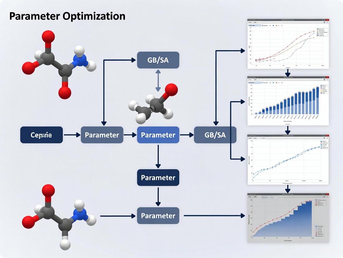
GB/SA Parameter Optimization Workflow
Advanced Applications and Methodologies
Machine Learning-Enhanced Implicit Solvation
Recent advances integrate graph neural networks (GNNs) with traditional implicit solvent approaches. The λ-Solvation Neural Network (LSNN) demonstrates how machine learning can overcome limitations of force-matching alone, which traditionally determined potential energies only up to an arbitrary constant. [5] These hybrid models achieve accuracy comparable to explicit-solvent alchemical simulations while maintaining computational efficiency of implicit models. [5]
Protocol: Machine Learning Implicit Solvent Implementation
- Network Architecture: Implement graph neural network that operates on molecular structures
- Multi-Term Loss Function: Train using combined force-matching and alchemical derivative terms
- Data Generation: Leverage large-scale explicit solvent simulations (~300,000 molecules) for training
- Model Validation: Test free energy predictions against experimental and explicit solvent reference data
Hybrid Explicit-Implicit Solvation
For systems where specific solvent interactions are critical, hybrid approaches provide a balanced solution:
Hybrid Solvation Model Structure
Research Reagent Solutions
Table: Essential Computational Tools for GB/SA Research
| Tool/Parameter | Function | Implementation Example |
|---|---|---|
| GB Model Kernels | Calculate electrostatic solvation | Still GB [7], GBSW [6] |
| SASA Calculators | Compute non-polar contributions | POPS [2], Fast SASA algorithms |
| Reference Data Sets | Parameterization and validation | Experimental hydration free energies [4] |
| Force-Matching Scripts | Optimize parameters | Custom loss function minimization [5] |
| Validation Suites | Benchmark performance | Test sets with diverse molecules [4] |
| ALPB/GBSA Solvers | Numerical implementation | xtb [7], AMBER, CHARMM |
| Lebedev Grids | SASA numerical integration | Multiple resolution levels [7] |
Frequently Asked Questions
Can implicit solvent models reproduce explicit solvent conformational ensembles? For some systems like the PHF6 peptide, implicit solvents (GB, GBSW, EEF1) can generate potential energy minima and free energy profiles in good agreement with explicit solvent simulations. [6] However, limitations exist, particularly for systems dependent on specific water-mediated interactions, where implicit models may alter conformational preferences. [1]
How do I choose between PB, GB, and SASA models? Selection criteria include:
- Poisson-Boltzmann: High accuracy electrostatic calculations when computational cost is secondary
- Generalized Born: Molecular dynamics simulations requiring balance of speed and accuracy
- SASA-based models: Rapid screening applications or coarse-grained simulations
What are the key limitations of current GB/SA models? Major challenges include: handling of nucleic acids and membranes; describing specific hydrogen-bonding interactions; accounting for solvent viscosity effects; and balancing polar/non-polar terms to avoid systematic biases. [2] [1] Machine learning approaches show promise in addressing these limitations. [5]
How important are atomic radii parameterizations? Born radii calculations are critically important as they directly impact the electrostatic component of solvation energy. Small changes (0.1Å) can significantly alter predicted solvation energies. Volume-integration methods generally outperform pairwise approximations for Born radii calculation. [3]
Can GB/SA models handle non-aqueous solvents? Yes, parameterizations exist for organic solvents like octanol, chloroform, and DMSO. The xtb package, for instance, provides parameters for numerous solvents including acetone, acetonitrile, DMSO, and ethanol. [7] However, accuracy may vary, and specific parameterization for target solvents is recommended.
Frequently Asked Questions
FAQ 1: My calculated solvation free energies for small, polar molecules are consistently too positive. What could be the cause? This issue often originates from an underestimation of the polar component (ΔGelec). First, verify the Generalized Born (GB) model parameters and the internal dielectric constant assigned to the solute. An incorrect or suboptimal set of numerical parameters within the GB model can lead to poor estimation of effective Born radii, which in turn miscalculates the screening of electrostatic interactions [8]. Second, ensure the partial atomic charges of your solute are accurate, as they directly influence the electrostatic potential; using methods like AM1-BCC has been shown to yield good agreement with experimental data [8].
FAQ 2: How can I improve the poor correlation between calculated and experimental solvation free energies for a diverse set of molecules? A poor overall correlation frequently points to problems with the nonpolar component (ΔGnp). The nonpolar term is often computed as a solvent-accessible surface area (SASA) term scaled by a surface tension coefficient. Using a single, global surface tension parameter for all atom types is a common source of error. Implementing atom type-dependent surface tension coefficients can significantly improve accuracy, as this better captures the physics of dispersive and cavitation interactions [4]. Furthermore, for more sophisticated analyses, consider models that further separate the nonpolar energy into repulsive and attractive contributions [9].
FAQ 3: My geometry optimization in an implicit solvent fails to converge. What steps can I take?
Non-convergence can be related to numerical noise in the solvation energy calculation. Try increasing the integration grid size used for calculating the surface area term. For example, in the xtb program, switching from a normal grid (230 points) to a tight grid (974 points) or higher can reduce noise and aid convergence [7]. Additionally, confirm that the cavity surface definition (e.g., Solvent-Excluding Surface vs. Solvent-Accessible Surface) is appropriate for your system and is being generated correctly by the software [10] [11].
FAQ 4: Why do my solvation free energy calculations for dimer complexes show large errors compared to explicit solvent benchmarks? While implicit models can perform well for monomer solvation free energies, dimers present a more challenging case. The model may struggle to accurately reproduce the relative nonpolar free energy landscapes near the global minimum of the complex [9]. This highlights a limitation of some standard implicit solvent models for capturing all the nuances of association processes. For such systems, it is advisable to validate your implicit model results against explicit solvent calculations or experimental data for similar complexes before drawing firm conclusions.
Troubleshooting Guides
Issue: Inaccurate Polar Solvation Energy (ΔGelec)
Problem Identification: The electrostatic component of the solvation free energy is inaccurate, leading to deviations from reference data (experimental or high-level explicit solvent calculations).
Resolution Protocol:
- Diagnosis: Perform a calculation on a set of small molecules with known solvation free energies. If the error correlates with molecular polarity, the issue likely lies with the ΔGelec term.
- Parameter Check:
- Model Upgrade: If available, try a different, more modern implicit solvent model. For example, the PME-GIST method, which incorporates long-range electrostatic and Lennard-Jones interactions more consistently with modern molecular dynamics engines, has shown exceptional agreement with thermodynamic integration (TI) (R² = 0.99) [12] [13].
- Advanced Consideration: For quantum chemistry calculations, explore the use of the Gaussian Charge Scheme in continuum models like C-PCM, which can offer improved numerical stability over point charges [10] [11].
Issue: Inaccurate Nonpolar Solvation Energy (ΔGnp)
Problem Identification: The nonpolar component is not accurately capturing cavitation and dispersion interactions, often evident as systematic errors for hydrophobic molecules.
Resolution Protocol:
- Term Decomposition: Investigate if your model can separate the nonpolar term into repulsive (cavitation) and attractive (dispersion) components. Correlating the repulsive free energy with molecular surfaces or volumes has been shown to achieve correlation coefficients higher than 0.99 with explicit solvent [9].
- Refine SASA Parameters: If using a SASA-based model, optimize the surface tension coefficient (γ). Better yet, implement atom-specific surface tension coefficients. Research has demonstrated that this approach can bring implicit solvent model accuracy to a level comparable with explicit TIP3P water models [4].
- Explore Advanced Models: Consider using more sophisticated nonpolar models. Differential Geometry (DG) based solvation models avoid ad hoc surface definitions and geometric singularities, dynamically coupling polar and non-polar interactions. After parameter optimization, these models have achieved an overall RMSE of 0.5 kcal/mol for a wide range of molecules [14].
Experimental Protocols & Data
Table 1: Performance of Solvation Free Energy Calculation Methods
Table comparing the accuracy and key features of different computational approaches for predicting solvation free energies.
| Method / Model Name | Key Features | Target Systems | Reported Accuracy (vs. Experiment) | Reference |
|---|---|---|---|---|
| GBSA (OBC2) | Generalized Born + SASA; common in MD packages | Small neutral molecules | AUE* = 1.1-1.4 kcal/mol, R² = 0.66-0.81 | [8] |
| PME-GIST | Grid-based; maps thermodynamics; uses PME | Small hydrophobic/hydrophilic molecules | MUE = 1.4 kcal/mol, R² = 0.88 | [12] [13] |
| DG-based Solvation | Differential geometry; smooth solute-solvent interface | Polar & non-polar molecules | RMSE* = 0.5 kcal/mol | [14] |
| GBSA (Atomistic γ) | GB + SASA with atom-type specific surface tensions | Small organic molecules | Comparable to explicit TIP3P | [4] |
| ALPB (in xTB) | Analytical linearized Poisson-Boltzmann; for semiempirical methods | Organic molecules in various solvents | N/A (Integrated in xTB Hamiltonian) | [7] |
*Average Unsigned Error; Mean Unsigned Error; *Root Mean Square Error
Protocol 1: Validating Solvation Free Energy Components Using End-State Analysis
This protocol outlines how to use the PME-GIST method to decompose and validate solvation free energy components [12].
- System Preparation:
- Obtain the 3D structure of the solute molecule.
- Parametrize the solute using a force field (e.g., GAFF2) and assign partial charges (e.g., with AM1-BCC).
- Solvate the solute in a rectangular TIP3P water box, ensuring a minimum distance of 15 Å between the solute and box edges.
- Molecular Dynamics Simulation:
- Minimize the system and equilibrate under NPT conditions (250 ps, 300 K, 1 bar).
- Run a production MD simulation (e.g., 100 ns) with all solute atoms harmonically restrained. Use a tool like Amber's
PMEMDwith Particle Mesh Ewald (PME) for electrostatics. - Save simulation frames regularly (e.g., every 2 ps) for analysis.
- GIST Analysis:
- Use the
CPPTRAJsoftware with the PME-GIST implementation. - Define a cubic grid centered on the solute with high resolution (e.g., 0.125 ų per voxel) that covers the entire system.
- Run the GIST analysis on the saved trajectory. The output will map the energy and entropy contributions of the solvent onto the grid.
- Use the
- Data Interpretation:
- The sum over all grid voxels provides the total solvation energy and the first-order entropy.
- Compare the PME-GIST calculated solvation energy to a TI benchmark. High correlation (R² = 0.99) validates the energy component [12].
- For entropy, note that GIST typically truncates the N-body expansion. A simple linear scaling correction can be applied to account for higher-order terms, which significantly improves the free energy correlation with TI (R² = 0.99) [12].
Protocol 2: Parameter Optimization for Differential Geometry Solvation Models
This protocol describes the steps for achieving an optimal parametrization in DG-based solvation models, which is crucial for their accuracy [14].
- Free Energy Functional Setup:
- The total free energy functional is defined, integrating terms for surface tension (γ|∇S|), pressure (pS), van der Waals interactions ((1-S)U), and electrostatic contributions from both solute and solvent domains.
- Coupled PDE Solution:
- Solve the coupled system of nonlinear geometric partial differential equations derived from the variation of the free energy functional: the Generalized Laplace-Beltrami (GLB) equation and the Generalized Poisson-Boltzmann (GPB) equation.
- Stabilization and Optimization:
- Apply Physical Constraints: Prescribe conditions to ensure the physical solution of the GLB equation, which promotes the well-posedness of the GPB equation.
- Use Perturbation Theory: Implement parameter learning algorithms based on perturbation and convex optimization theories to stabilize the iterative numerical solution of the coupled PDEs.
- Parameter Optimization: The achieved stability allows for the systematic optimization of model parameters (like surface tension and pressure) against a database of experimental solvation free energies for a diverse set of molecules.
Diagram 1: DG model optimization workflow.
The Scientist's Toolkit
Table 2: Essential Research Reagents & Software Solutions
A table of key software tools and models used in the development and application of implicit solvent models.
| Item Name | Type / Category | Primary Function | Key Application in Research |
|---|---|---|---|
| AMBER | Molecular Dynamics Suite | Performs MD, TI, and FEP simulations. | Generates reference data (via TI) and trajectories for GIST analysis [12]. |
| CHARMM | Molecular Dynamics Suite | Simulates biomolecular systems with various force fields. | Platform for testing and applying different GB models and parameters [8]. |
| ORCA | Quantum Chemistry Package | Ab initio quantum chemistry calculations. | Implements implicit solvent models (C-PCM, SMD) for electronic structure calculations in solution [10] [11]. |
| xtb | Semiempirical Quantum Chemistry | Fast quantum mechanical calculations. | Provides the ALPB and GBSA implicit solvation models for the GFN family of Hamiltonians [7]. |
| CPPTRAJ | Analysis Toolbox | Analyzes molecular dynamics trajectories. | The primary software environment for running GIST and PME-GIST analyses [12] [13]. |
| GBSA Model | Implicit Solvent Model | Approximates ΔGelec with GB and ΔGnp with SASA. | A widely used benchmark and base framework for parameter optimization studies [8] [4]. |
| DG-Based Model | Implicit Solvent Model | Uses differential geometry for a smooth solute-solvent boundary. | Provides a robust framework for accurate solvation free energy prediction without ad hoc parameters [14]. |
Troubleshooting Guides
Guide 1: Inaccurate Protein-Ligand Binding Affinity Predictions
Problem: Calculated binding free energies for protein-drug complexes show large deviations from reference Poisson-Boltzmann (PB) results or experimental data.
| Diagnostic Question | Likely Root Cause | Recommended Solution |
|---|---|---|
| Which GB model are you using? | Older GB models (e.g., GB-HCT, GB-OBC) may perform poorly for charged ligands [15]. | Switch to a more modern, surface-based GB model like GBNSR6 (GB-NSR6), which shows closest overall agreement with PB for binding free energies [15] [16]. |
| What is the net charge of the ligand? | High charge density can lead to an overestimation of the desolvation penalty [17]. | Systematically adjust the intrinsic radii (( \rho )) for key atoms involved in binding. Increasing ( \rho ) can enhance Coulomb bond stability [17]. |
| Are you using a coarse grid? | Grid artifacts can introduce errors of ~0.6 kcal/mol in binding free energy calculations [16]. | For grid-based GB models, ensure a grid spacing of 0.5 Å or finer to minimize numerical errors [16]. |
Guide 2: Unstable Coulombic (Ionic) Bonds in MD Simulations
Problem: Salt bridges or hydrogen bonds in simulated proteins or protein complexes break unexpectedly.
| Diagnostic Question | Likely Root Cause | Recommended Solution |
|---|---|---|
| What are your current intrinsic radii (( \rho )) settings? | Standard Bondi radii may overestimate the desolvation penalty, destabilizing charged interactions [17]. | Increase the intrinsic radii (( \rho )) for hydrogen and oxygen atoms involved in the bonds. This increases the low-dielectric region, enhancing attractive interaction energy [17]. |
| What is the value of your spatial integration cutoff (( r_{max} ))? | A large ( r_{max} ) can overestimate the desolvation penalty, making bond formation less favorable [17]. | Use a relatively small ( r_{max} ) in combination with larger intrinsic radii for a more accurate balance [17]. |
Guide 3: Poor Performance on RNA-Peptide or Membrane Protein Systems
Problem: The GB model fails to reproduce electrostatic behavior for RNA, peptides, or membrane-embedded systems.
| Diagnostic Question | Likely Root Cause | Recommended Solution |
|---|---|---|
| Is your system an RNA-peptide complex? | These are among the most challenging cases for most standard GB models [15]. | Validate your results against a reference PB calculation for your specific system. The GBNSR6 model is one of the few that performs robustly across diverse complexes [15]. |
| Are you simulating a membrane protein? | Standard GB models are parameterized for bulk water, not heterogeneous membrane environments [18]. | Use a specialized implicit membrane GB model that treats the membrane as an infinite planar low-dielectric slab [18]. |
Frequently Asked Questions (FAQs)
Q1: What is the fundamental difference between the Poisson-Boltzmann (PB) and Generalized Born (GB) methods?
Both are implicit solvent models that treat the solvent as a continuum. The PB equation is a more rigorous (but computationally expensive) approach that is often used as a reference for accuracy [15] [19]. The GB model is a highly efficient approximation to PB, making it suitable for molecular dynamics simulations and high-throughput calculations [15] [19] [16].
Q2: I need to choose a GB model for my project. Which one should I use?
Your choice should balance accuracy and computational cost. Based on a systematic evaluation of 60 biomolecular complexes [15]:
- For the highest overall accuracy in binding free energy calculations, use a surface-based "R6" model like GBNSR6.
- For small neutral complexes, most common GB models (GB-HCT, GB-OBC, etc.) perform adequately.
- Be aware that performance varies significantly across complex types, with protein-drug and RNA-peptide complexes being particularly challenging for many models.
Q3: What is the "intrinsic radius" in a GB model, and why is it important?
The intrinsic radius (( \rho )) is a key parameter that defines the dielectric boundary for an atom—essentially, where the solute ends and the solvent begins [17]. It is critically important because:
- It is not just a fixed atomic radius (like the Bondi radius); it is a parameter that can be optimized.
- Adjusting ( \rho ) directly affects the stability of Coulombic bonds (like salt bridges and hydrogen bonds). Increasing ( \rho ) enhances bond stability by improving the interaction energy term [17].
Q4: My machine learning-based implicit solvent model predicts forces well but gives poor absolute free energies. Why?
This is a known limitation of models trained solely on force-matching. Force-matching determines energies only up to an arbitrary constant, making the predictions unsuitable for absolute free energy comparisons [5]. A solution is to extend the training to include derivatives of the solvation energy with respect to alchemical coupling parameters (( \lambda )), which ties the model to a defined energy scale [5].
Q5: Can the standard Born equation accurately describe all ions in solution?
The classical Born equation has limitations. Recent research shows that the "Born radius" naturally emerges from accounting for dielectric saturation effects—the fact that the dielectric constant of the solvent is not uniform near a highly charged ion but becomes reduced [20]. Newer modifications, like the S-Born model, which include these effects and temperature-dependent corrections, show improved performance for solvation properties [20].
Experimental Protocols & Data
Protocol 1: Calculating Electrostatic Binding Free Energy with a GB Model
This protocol outlines the standard thermodynamic cycle for calculating the electrostatic component of binding free energy (( \Delta \Delta G_{el} )) [15] [16].
Protocol 2: Optimizing Intrinsic Radii for Coulomb Bond Stability
This methodology is used to systematically adjust the intrinsic radius (( \rho )) parameter to stabilize specific ionic or hydrogen bonds in a structure [17].
Quantitative Model Performance Data
Table 1: Accuracy of GB Models in Reproducing PB Electrostatic Binding Free Energies (Across 60 diverse biomolecular complexes [15])
| GB Model | Correlation with PB (R²) | RMSD (kcal/mol) | Performance Notes |
|---|---|---|---|
| GBNSR6 (GB-NSR6) | 0.9949 | 8.75 | Closest overall agreement with PB |
| GB-HCT | 0.9444 | 16.02 | Lower accuracy for charged systems |
| GB-OBC | 0.9616 | 13.86 | Moderate performance |
| GB-neck2 | 0.9308 | 17.26 | Challenged by RNA-peptide & protein-drug complexes |
| Performance Range | 0.3772 - 0.9986 | Varies Widely | Highlights need for careful model selection |
Table 2: Parameter Adjustment Guide for Coulomb Bond Stability [17]
| Parameter | Default Value (Approx.) | Effect of Increasing | Underlying Physical Mechanism | Recommended Use |
|---|---|---|---|---|
| Intrinsic Radius (( \rho )) | Bondi radius (e.g., H: 1.1-1.2 Å) | Enhances stability | Increases low-dielectric region, boosting favorable interaction energy | To stabilize specific salt bridges or hydrogen bonds |
| Spatial Integral Cutoff (( r_{max} )) | Model-dependent | Can decrease stability | Overestimates desolvation penalty upon binding | Use a relatively small value in combination with larger ( \rho ) |
The Scientist's Toolkit
Table 3: Essential Research Reagents & Computational Tools
| Item | Function in GB/SA Research | Key Considerations |
|---|---|---|
| GB Model Software | Provides the engine for calculating electrostatic solvation energies. | Major MD packages (AMBER, CHARMM, NAMD) implement multiple GB flavors [15]. |
| Poisson-Boltzmann Solver | Serves as a reference for assessing GB model accuracy [15] [16]. | Use highly accurate solvers like MIBPB [16] or APBS [21]. |
| Molecular Structure Files (PQR) | Input files containing atomic coordinates, charges, and radii. | Radii parameters in this file are critical for defining the dielectric boundary [21]. |
| Intrinsic Radius (( \rho )) | A tunable parameter to optimize electrostatic interactions. | Systematic adjustment is key for stabilizing Coulomb bonds in specific contexts [17]. |
| Machine Learning Correctors | New tools to improve the accuracy of traditional GB/PB models. | Models like LSNN are trained to match energy derivatives for accurate free energies [5]. |
Frequently Asked Questions (FAQs)
Q1: What is the fundamental physical meaning of the SASA term in an implicit solvent model? The Solvent-Accessible Surface Area (SASA) model approximates the nonpolar component of the solvation free energy (ΔGnp). This nonpolar term primarily represents the thermodynamic cost of forming a cavity in the solvent to accommodate the solute molecule (ΔGcav) and the van der Waals dispersion interactions between the solute and solvent (ΔGvdW) [19] [2]. In practice, the model assumes these contributions are proportional to the surface area of each atom exposed to the solvent [22].
Q2: My GB/SA simulation is slow. What is the primary computational bottleneck and how can I address it? The calculation of the precise SASA for each atom at every simulation step is often the bottleneck, as it is not pair-wise decomposable and depends on the entire molecular geometry [23]. To improve performance, you can:
- Use an analytical approximation: Switch from a numerical "rolling ball" algorithm (e.g., Shrake-Rupley) to a faster analytical Linear Combination of Pairwise Overlaps (LCPO) method, though this may introduce a small error (1-3 Ų) [24].
- Coarsen the SASA grid: If using a numerical method, reduce the grid level (e.g., from
verytighttonormal), which decreases the number of points used to probe the surface, thereby speeding up the calculation at the cost of increased numerical noise [7].
Q3: My geometry optimization fails to converge with the SASA model enabled. What could be wrong? This is frequently caused by excessive numerical noise in the SASA energy gradient [7]. To resolve this:
- Tighten the SASA grid: Use a finer grid (e.g.,
tightorverytight) to reduce discretization noise and provide smoother gradients for the optimizer [7]. - Inspect atomic SASA values: Check for sudden, large changes in the SASA of individual atoms during the optimization, which can indicate problematic clashes or unrealistic conformations [7].
Q4: How do I parameterize the SASA model for a new molecule or force field? Parameterization involves determining atom-specific solvation parameters (σ_i). Common strategies include [2] [22]:
- Force Matching: Using large-scale explicit solvent simulations as a reference to fit the σ_i parameters so that the implicit solvent forces match the explicit ones.
- Trial and Error for Stability: Adjusting parameters to minimize the root mean square deviation from a known native state in molecular dynamics simulations [22].
- Free Energy of Transfer: Deriving parameters from experimental data on the free energy of transfer of small molecules between different solvents [2].
Troubleshooting Guide
| Problem Symptom | Likely Cause | Recommended Solution |
|---|---|---|
| Unstable simulation; protein unfolds. | Incorrect balance between polar and nonpolar terms or inaccurate SASA parameters [22]. | Re-parameterize the SASA surface tensions (σ_i) for your specific force field and validate against a known stable structure [22]. |
| Unphysical accumulation of hydrophobic residues on the molecule's surface. | The hydrophobic solvation parameter (σ_hydrophobic) is too weak, providing insufficient penalty for exposure. | Increase the value of the hydrophobic surface tension parameter (σ_hydrophobic) to strengthen the driving force for burial [22]. |
| Calculation crashes due to "undefined atom type". | The simulation software lacks SASA parameters for specific atoms in your molecule [22]. | Manually assign meaningful SASA parameters (radius, solvation parameter) for the unsupported atom types in the input script [22]. |
| Inaccurate binding free energies for protein-ligand complexes. | The SASA model fails to capture specific interactions like water bridging or entropic effects [19]. | Consider a hybrid approach: use a more detailed model like Poisson-Boltzmann (PB) for final energy evaluation or apply a machine-learning-based correction [19]. |
▼ Table of SASA Approximation Algorithms and Performance
The choice of SASA calculation algorithm involves a direct trade-off between computational speed and accuracy. The following table summarizes different methods used in biophysical simulations [24] [23].
| Algorithm Type | Key Principle | Computational Speed | Typical Error (vs. Numerical) | Best Use Case |
|---|---|---|---|---|
| Shrake-Rupley (Numerical) | Rolls a spherical probe (1.4 Å) over a mesh of points on the van der Waals surface [24]. | Slow | Reference Standard | Final analysis; high-accuracy single-point calculations. |
| LCPO (Analytical) | Linear Combination of Pairwise Overlaps; provides an analytical approximation [24]. | Fast | 1 - 3 Ų [24] | Production molecular dynamics simulations. |
| Neighbor Vector | Accounts for spatial orientation of neighboring atoms to estimate burial [23]. | Medium | Lower than density-based | Protein structure prediction where orientation matters. |
| Neighborhood Density | Counts atoms/centroids within a spherical cutoff (e.g., 10-14 Å) [23]. | Very Fast | Varies, can be significant | Early-stage high-throughput screening in de novo folding. |
▼ Research Reagent Solutions
| Essential Material / Software | Function in SASA Modeling |
|---|---|
| CHARMM | A versatile program for atomic-level simulation that implements the SASA model for implicit solvation, enabling folding studies of peptides and miniproteins [22]. |
| xtb | A semi-empirical quantum chemistry program that includes the GBSA/ALPB implicit solvation models, allowing for rapid geometry optimization and energy calculations in solution [7]. |
| AMBER | A molecular dynamics software package that employs the LCPO method for efficient analytical calculation of SASA during simulations [24]. |
| POPS & POPSCOMP | Fast computational methods for SASA analysis of proteins, nucleic acids, and their complexes, useful for parameterization and analysis [2]. |
Modified Parameter Files (e.g., param19_eef1.inp) |
Specialized parameter files that neutralize formal charges on ionic side chains and termini, which are required for the proper functioning of certain SASA models within force fields [22]. |
Workflow for SASA Model Parameterization and Application
The following diagram outlines a general workflow for developing and applying a SASA model in biomolecular research, integrating steps from parameterization to troubleshooting.
SASA Calculation and Evaluation Logic
This diagram illustrates the logical decision process for selecting a SASA approximation method based on the researcher's goal, highlighting the trade-off between speed and accuracy.
Frequently Asked Questions (FAQs)
Q1: What are the foundational theories behind modern implicit solvent models like GB/SA? The conceptual foundation of implicit solvent models lies in early dielectric theories of solvation. The seminal work of Lars Onsager and Peter Debye in the early 20th century established the treatment of solvents as dielectric continua, enabling the estimation of solvation energies based on bulk properties like dielectric constant and molecular polarizability [19]. Onsager's specific contribution was a model to refine the Lorentz local field approximation in a system of dipoles [19]. These early continuum models laid the groundwork for the development of the Poisson-Boltzmann equation and, later, the more efficient Generalized Born (GB) approximation [19].
Q2: My binding free energy calculations are sensitive to the choice of GB model. How do I select the right one?
The accuracy of Generalized Born (GB) models can vary significantly depending on the type of biomolecular complex being studied [15]. It is crucial to select a GB model that has been validated for systems similar to yours. For instance, a study comparing eight common GB flavors found that their performance varied across different complex types [15]. The GB-neck2 model, for example, showed the closest overall agreement with the reference Poisson-Boltzmann method in one benchmark [15]. The table below summarizes the relative performance of different GB models across various complex types. Using a model inappropriate for your system (e.g., using a model calibrated for proteins on an RNA complex) is a common source of error.
Q3: Why are my MM/GBSA results inconsistent when I use the 3-average (3A) approach instead of the 1-average (1A) approach? The 1-average (1A-MM/GBSA) approach, which uses only a simulation of the complex, often provides more precise results (smaller standard error) compared to the 3-average (3A-MM/GBSA) approach, which requires separate simulations for the complex, receptor, and ligand [25]. The 3A approach can lead to very large uncertainties because the conformational ensembles for the unbound receptor and ligand are sampled independently, which can introduce noise [25]. However, the 1A approach ignores changes in the structure of the ligand and receptor upon binding. The best practice is to test both methods for your specific system if computationally feasible, but be aware that the 3A approach typically has a much higher computational cost and may yield larger uncertainties [25].
Q4: What are the primary limitations of the MM/GBSA method that I should account for in my analysis? MM/GBSA contains several notable approximations [25]:
- Conformational Entropy: The entropy contribution, often estimated by normal-mode analysis, is computationally expensive and is sometimes omitted, leading to incomplete free energy estimates.
- Solvent Representation: The continuum solvent model cannot capture specific, atomistic solvent effects such as water bridges or specific hydrogen bonds in the binding site.
- Internal Enthalpy: The method typically uses the gas-phase molecular mechanics energy, which does not include the polarizable environment in its internal energy terms.
- Standard State: Early formulations omitted corrections for the translational and rotational enthalpy, and care must be taken to use a 1 M standard state for the translational entropy to match experimental conditions [25].
Q5: How can I incorporate multiple objectives, like binding affinity and drug-likeness, into my generative molecular design process? Traditional target-aware generative models often focus on a single objective, such as binding affinity. To simultaneously optimize multiple properties, you can employ multi-objective optimization algorithms. One such method is Pareto MCTS, which searches for molecules on the "Pareto Front"—the set of molecules where no single property can be improved without worsening another [26]. This approach allows for the balancing of competing objectives, such as docking score, quantitative estimate of drug-likeness (QED), and synthetic accessibility (SA) score, during the molecule generation process itself [26].
Troubleshooting Guides
Issue 1: Inaccurate Electrostatic Binding Free Energy Calculations
Problem Calculated electrostatic binding free energies (ΔΔG_el) deviate significantly from reference data or Poisson-Boltzmann (PB) results, or show poor correlation across a series of ligands [15].
Solution
- Benchmark your GB Model: Do not assume all GB models perform equally. Consult benchmark studies to identify the best-performing GB model for your specific class of biomolecular complex (e.g., protein-protein, protein-drug, RNA-peptide) [15].
- Validate with PB: If possible, use a PB solver as a reference to calibrate your GB results for a subset of your systems. A large discrepancy indicates the GB model may be a poor fit [15].
- Check System Preparation:
- Atomic Radii: Ensure you are using the recommended set of atomic radii for your chosen GB model, as this parameter is highly sensitive [19].
- Dielectric Constant: Verify the internal and external dielectric constants. The standard values are 1 for the solute and 80 for the solvent, but these can be adjusted for specific contexts.
- Net Charge: Be aware that the accuracy of GB models can be influenced by the net charge of the system [15].
Issue 2: Poor Performance in Virtual Screening and Ligand Ranking
Problem MM/GBSA fails to correctly rank the potency of a series of ligands or cannot distinguish binders from non-binders.
Solution
- Re-evaluate the Decomposition: Use energy decomposition to check if the failure is systematic for a particular type of interaction (e.g., electrostatic, van der Waals). This can provide clues for further optimization.
- Inspect Conformational Sampling: Ensure your input MD simulation or conformational ensemble is adequately sampled. Insufficient sampling of bound-state geometries is a common cause of failure. Consider whether the simulation length is sufficient for the ligand and binding site.
- Consider the 2A Approach: If the 1A approach gives poor results, but the full 3A is too costly, try a 2A approach. This involves sampling the complex and the free ligand, which can help account for the ligand's reorganization energy upon binding [25].
- Test a Multi-Model Approach: Do not rely on a single implicit solvent model. If the computational budget allows, run your screening protocol with 2-3 different well-validated GB models and compare the consensus rankings.
Issue 3: Handling Challenging Systems like RNA and Highly Charged Complexes
Problem GB models show particularly large errors for RNA-peptide complexes or systems with high net charge [15].
Solution
- Acknowledge the Limitation: Recognize that some system types are inherently more challenging for GB approximations. RNA-peptide and protein-drug complexes have been noted as particularly difficult for many standard GB models [15].
- Use a Specialized Model: Select a GB model that has been specifically developed or shown to perform well for nucleic acids or highly charged systems, such as the
GB-neck2model [15]. - Fall Back to PB/SA: For these challenging cases, the more computationally demanding PB/SA method may be necessary for reliable results.
Experimental Protocols & Data
Table 1: Key Historical Milestones in Implicit Solvation
| Year/Period | Scientist/Model | Key Contribution | Impact on Modern GB/SA |
|---|---|---|---|
| Early 20th Century | Lars Onsager & Peter Debye | Pioneered dielectric theory of solvation; Onsager introduced a model for a system of dipoles [19]. | Laid the theoretical foundation for treating the solvent as a continuous dielectric medium. |
| 1931 | Lars Onsager | Formulated the Onsager reciprocal relations, fundamental to the thermodynamics of irreversible processes [27] [28]. | Provided the rigorous thermodynamic basis for non-equilibrium processes underlying solvation dynamics. |
| 1990s | Kollman et al. | Developed the MM/PBSA and MM/GBSA end-point free energy methods [25]. | Established the primary computational framework for using GB/SA models in binding affinity calculations. |
| 2000s - Present | Various Groups | Development of numerous GB "flavors" (e.g., GB-HCT, GB-OBC, GB-neck2, GBNSR6) [15]. | Offered a range of accuracy/speed trade-offs, allowing application to larger systems and longer timescales. |
| 2010s - Present | Machine Learning & Multi-Objective Optimization | Integration of ML correctors and Pareto front optimization for multi-property molecule design [19] [26]. | Pushes the frontier towards higher accuracy and the simultaneous optimization of affinity, drug-likeness, and other key properties. |
Table 2: Performance of GB Models Across Biomolecular Complex Types (Relative to PB Reference)
This table summarizes findings from a systematic assessment of eight GB models. The performance is measured by the correlation (R²) and root-mean-square deviation (RMSD) of electrostatic binding free energies compared to a Poisson-Boltzmann reference [15].
| GB Model | Small Neutral Complexes | Protein-Protein Complexes | Protein-Drug Complexes | RNA-Peptide Complexes |
|---|---|---|---|---|
| GB-HCT | Moderate Accuracy | Lower Accuracy | Challenging | Most Challenging |
| GB-OBC | Moderate Accuracy | Moderate Accuracy | Challenging | Challenging |
| GB-neck2 | High Accuracy | High Accuracy | Less Challenging | Less Challenging |
| GBNSR6 | High Accuracy | High Accuracy | Challenging | Challenging |
| General Trend | Least challenging for most models. | Performance varies widely. | High net charge and complexity make this class difficult. | Most challenging for all but one model (GB-neck2). |
Workflow 1: Standard MM/GBSA Protocol for Ligand Binding Affinity
Detailed Methodology:
- System Setup: Prepare the protein-ligand complex, the free protein, and the free ligand. Ensure proper protonation states and assign force field parameters.
- Sampling: Perform molecular dynamics (MD) simulations for each state (complex, receptor, ligand) in explicit solvent to generate conformational ensembles. Alternatively, for the 1A approach, run only the complex simulation [25].
- Post-Processing: For each saved snapshot from the trajectory, remove all explicit water molecules and ions.
- Energy Calculation: For each snapshot, calculate the following components [25]:
- Gas-Phase MM Energy: The internal (bond, angle, dihedral), electrostatic, and van der Waals energy of the molecule.
- Polar Solvation Energy (Gpol): Using a GB model to solve the electrostatics.
- Non-Polar Solvation Energy (Gnp): Typically calculated as a linear function of the Solvent Accessible Surface Area (SASA), γ*SASA + b.
- Entropy Estimation: Calculate the conformational entropy change upon binding, often using quasi-harmonic or normal-mode analysis. Note: This step is computationally expensive and is sometimes omitted.
- Free Energy Calculation: Combine the terms for each state and compute the binding free energy using the formula: ΔGbind = Gcomplex - (Greceptor + Gligand), where G = EMM + Gsolv - TS.
- Averaging: Average the calculated ΔG_bind over all snapshots to obtain the final estimate and its standard error.
Workflow 2: Multi-Objective Optimization for Molecular Design
Detailed Methodology:
- Initialization: Begin with a pre-trained, target-aware generative model (e.g., a variational autoencoder or autoregressive model) and a set of target properties (e.g., docking score, QED, SA score) [26].
- Generation: Use the model to generate an initial population of molecules.
- Evaluation: Calculate all target properties for each generated molecule.
- Pareto Analysis: Identify the "Pareto-optimal" molecules—those for which no other molecule is better in all properties simultaneously. This set forms the "Pareto Front" [26].
- Iterative Optimization: Use a search algorithm (e.g., Monte Carlo Tree Search with a scheme like ParetoPUCT) to guide the generative model towards regions of chemical space that improve upon the current Pareto Front. This balances exploration of new structures with the exploitation of known promising areas [26].
- Convergence: Repeat steps 2-5 until a stopping criterion is met (e.g., number of iterations or no improvement in the Pareto Front).
- Output: The final output is a set of molecules on the Pareto Front, providing a range of optimal trade-offs between the multiple desired properties.
The Scientist's Toolkit: Key Research Reagents & Materials
| Item / Software | Function / Role in Research |
|---|---|
| Molecular Dynamics Engines (AMBER, CHARMM, GROMACS) | Software packages used to run MD simulations that generate the conformational ensembles for MM/GBSA calculations. They contain implementations of various GB models [15]. |
| GB Model "Flavors" (GB-OBC, GB-neck2, GBNSR6) | Different algorithmic implementations of the Generalized Born approximation. They represent the core "reagent" for calculating the polar solvation energy and have different accuracy/speed characteristics [15]. |
| Poisson-Boltzmann Solver (e.g., APBS, DelPhi) | Software used to numerically solve the PB equation. It is often used as a more accurate reference method to benchmark the results from faster GB models [19] [15]. |
| SASA Calculator | A tool to compute the Solvent Accessible Surface Area. This value is used to estimate the non-polar component of the solvation free energy (G_np) [25]. |
| Normal-Mode Analysis Tool | A program to calculate vibrational frequencies from a molecular structure, which can be used to estimate the conformational entropy contribution (-TS) to the binding free energy [25]. |
| Docking Score Function (e.g., smina) | A tool to quickly predict the binding affinity and pose of a ligand in a protein binding site. Used as one of the objectives in multi-objective optimization workflows [26]. |
| Property Prediction Tools (for QED, LogP, SA Score) | Software or libraries that calculate key drug-like properties, enabling the multi-objective optimization of generated molecules beyond just binding affinity [26]. |
Frequently Asked Questions (FAQs)
Q1: What is the fundamental difference between the van der Waals (vdW) and Molecular Surface (MS) definitions of the dielectric boundary? The key difference lies in the treatment of the interstitial space between atoms.
- Van der Waals (vdW) Surface: Formed by the union of hard spheres representing individual atoms using their van der Waals radii. This surface treats any tiny crevasse between atoms as filled with high-dielectric solvent [29] [30].
- Molecular Surface (MS) / Solvent-Excluded Surface (SES): Defined by rolling a spherical probe (representing a solvent molecule) over the vdW surface. The MS comprises the contact surface (where the probe touches the vdW surface) and the re-entrant surface (the inward-facing parts of the probe when it contacts multiple atoms) [30]. This surface treats the entire molecular interior as a low-dielectric region, excluding spaces too small for the solvent probe to enter [29].
Q2: I am simulating small organic molecules. Which dielectric boundary is recommended for the most accurate electrostatic solvation energy (ΔGel)? For small molecules, a dielectric boundary based on the van der Waals surface with optimally shifted atomic radii can yield accuracy comparable to, or even surpassing, the molecular surface definition. Research indicates that using the vdW surface with BONDI atomic radii uniformly increased by approximately 0.2 Å can produce highly accurate ΔGel estimates [29]. At this optimal setting, pairwise charge-charge interactions computed with the vdW boundary are virtually identical to those from the MS boundary.
Q3: When simulating proteins or peptides, is the vdW surface with shifted radii still the best choice? No. For structures larger than small molecules, the optimal dielectric boundary definition changes. The Molecular Surface (MS) is generally considered more physically realistic and provides superior accuracy for peptides and proteins [29]. While an optimal vdW surface (e.g., using a specific probe radius) might achieve a similar total ΔGel, the pairwise electrostatic interactions between individual atoms can show significant deviations (up to 5 kcal/mol for some pairs) compared to the MS result, which can critically impact conformational sampling and stability [29].
Q4: What is the Solvent Accessible Surface (SAS), and how does it relate to the vdW and MS definitions? The Solvent Accessible Surface (SAS) is defined by the path of the center of the spherical solvent probe as it is rolled around the solute molecule [31] [30]. Geometrically, the SAS is equivalent to the vdW surface where all atomic radii have been increased by the radius of the solvent probe [29]. It represents the outer limit of the region occupied by the solute and its surrounding first solvation shell.
Q5: Why is the choice of dielectric boundary so critical in implicit solvation calculations? The electrostatic solvation energy is highly sensitive to the position of the dielectric boundary. For a single atom, a shift of just 0.1 Å in the boundary can alter its solvation energy by as much as 10 kcal/mol, an energy comparable to the stability of a typical protein [29]. An inaccurate boundary can lead to misrepresentation of solvent screening, over- or under-stabilization of charged and polar groups (like over-stabilizing salt bridges), and ultimately, incorrect predictions of molecular structure, dynamics, and binding affinities [1] [29].
Troubleshooting Guides
Problem 1: Inaccurate Solvation Free Energies in Small Molecules
- Symptoms: Calculated solvation free energies for small, drug-like molecules consistently deviate from experimental or explicit solvent reference data.
- Investigation & Solution:
- Verify Boundary Definition: Check which surface definition your simulation package is using by default.
- Systematic Calibration: Perform a scan of the dielectric boundary parameter. If using a vdW-based definition, try simulating with atomic radii scaled by a series of small increments (e.g., from 0.0 Å to 0.4 Å). If using an MS definition, vary the solvent probe radius (ρw) around the typical value of 1.4 Å [29].
- Validate with Benchmark Set: Calculate ΔGel for a small set of molecules with known reference values. The table below summarizes optimal parameters found for small molecules [29].
Table 1: Optimal Dielectric Boundary Parameters for Small Molecules
| Surface Type | Atomic Radii Set | Probe Radius (ρw) | Optimal Adjustment | Expected Accuracy |
|---|---|---|---|---|
| Van der Waals | BONDI | Not Applicable | +0.2 Å | High; comparable to optimal MS |
| Molecular Surface | BONDI | ~1.2 Å (Varies) | Not Applicable | High |
| Solvent Accessible | BONDI | ~0.2 Å | Not Applicable | Comparable to optimal MS |
Problem 2: Poor Protein Folding or Unrealistic Salt Bridge Interactions
- Symptoms: Simulations of proteins or peptides result in non-native conformations, often characterized by an over-population of alpha-helices and an over-stabilization of salt bridges that do not persist in explicit solvent simulations [1].
- Investigation & Solution:
- Switch to Molecular Surface: This is the primary recommended action. The MS boundary provides a more physically realistic model of the protein-solvent interface, leading to better electrostatic screening and more accurate conformational ensembles [1] [29].
- Adjust Solute Dielectric Constant: If switching the boundary is computationally prohibitive, you can attempt to mimic the enhanced screening of the MS boundary within a vdW framework by increasing the solute's internal dielectric constant (εin). For small proteins, doubling εin from 1 to 2 can partially replicate the average reduction in pairwise interactions [29]. Note: This is a compromise and does not fix large individual deviations.
- Review Force Field Parameters: Ensure that your force field and implicit solvent model parameters (e.g., atomic radii) are consistent and designed to work together.
Experimental Protocols
Protocol: Benchmarking Dielectric Boundary Definitions for a Novel System
Objective: To empirically determine the most accurate dielectric boundary definition (vdW vs. MS) and its optimal parameterization for a given class of molecules (e.g., a new macrocyclic peptide) within a GB/SA model.
Workflow Overview:
The following diagram outlines the iterative protocol for benchmarking and selecting the optimal dielectric boundary.
Materials & Computational Setup:
Table 2: Research Reagent Solutions for Dielectric Boundary Benchmarking
| Item / Reagent | Function / Role in Protocol |
|---|---|
| Molecular Dynamics/Simulation Software (e.g., CHARMM, AMBER, GROMACS) | The computational engine for performing energy calculations and molecular dynamics simulations using the implicit solvent model. |
| Generalized Born (GB) Model | The specific implicit solvent model used to calculate the electrostatic component of solvation free energy (ΔGel) [3]. |
| Surface Area (SA) Term | The non-polar contribution to solvation free energy, often calculated as a linear function of the Solvent Accessible Surface Area (SASA) [1]. |
| Atomic Radii Set (e.g., BONDI, PARSE) | A consistent set of atomic van der Waals radii used as the baseline for defining the dielectric boundary [29]. |
| Benchmark Molecular Set | A curated set of molecules with reliable experimental or explicit solvent-derived solvation free energies for validation. |
| Solvent Probe Sphere | A geometric construct with a defined radius (typically 1.4 Å for water) used to generate the Molecular and Solvent Accessible Surfaces [30]. |
Methodology:
System Preparation:
- Obtain or generate 3D structures for your benchmark set. Ensure they are energetically minimized.
- Define the force field and atomic partial charges.
Parameter Scan Setup:
- For the vdW surface: Prepare a series of calculations where the base atomic radii set is scaled by an additive offset. A recommended range is from 0.0 Å to 0.4 Å in increments of 0.05 Å or 0.1 Å.
- For the Molecular Surface: Prepare a series of calculations where the solvent probe radius (ρw) is varied. A recommended range is from 1.0 Å to 1.8 Å [29].
Execution:
- For each parameter set in the scan, run a single-point energy calculation or a short minimization to compute the solvation free energy (ΔGsolv) for every molecule in the benchmark set.
Analysis:
- For each parameter set, calculate the average error and root-mean-square deviation (RMSD) between the computed ΔGsolv and the reference data.
- Plot the accuracy metrics (e.g., RMSD) against the varied parameter (radii offset or probe radius). The parameter set that minimizes the error is the optimal for your system and model.
- As a secondary check, examine the deviation of key pairwise electrostatic interactions (e.g., in a protein salt bridge) for the different boundaries, if such data is available [29].
Implementing and Applying GB/SA Models in Biomolecular Simulations
Troubleshooting Guides
Guide 1: Resolving Generalized Born Energy Discrepancies Between AMBER and OpenMM
Problem: Significant differences in the Generalized Born (GB) solvation energy term are observed when calculating the energy of the same molecular system using the same force field in AMBER and OpenMM, even after updating numerous GB parameters.
Investigation and Solutions:
- Confirm Parameter Transfer: Manually verify that all modified GB parameters have been correctly transferred and are active in the simulation. This includes parameters for GB atom radius, GB screening, GB neck scale, GB offset, and GB probe radius. Out of 27 GBNeck2 parameters, ensure all are updated, not just a subset [32].
- Check Underlying Models: Recognize that even with the same
igbsetting (e.g.,igb=5for the OBC model), the specific GBSA-OBC parameters implemented in OpenMM's internal force fields may differ from those found in the native AMBER application. Using AMBER-generatedparm7files with OpenMM's IGB2/5 might therefore lead to inconsistencies [33]. - Validate with Simple Systems: Test the parameter set on a small, well-characterized molecule (like a single amino acid) where reference GB energies are available, to isolate the issue.
- Recommended Action: When using the GBNeck2 model or its derivatives, the most reliable approach is to use the simulation software for which the force field was primarily developed and parameterized. If cross-software validation is essential, use the software-specific XML files provided by the force field developers instead of converted parameter files [33] [32].
Guide 2: Enabling GBNSR6 in MMPBSA.py for AMBER Simulations
Problem: When running MMPBSA.py with igb=6 (intended for the GBNSR6 model) in the input file, the output log states that Generalized Born ESURF is being calculated using 'LCPO' surface areas, instead of the expected GBNSR6 method [34].
Investigation and Solutions:
- Root Cause: The
igb=6setting controls the Generalized Born model itself, but the method for calculating the solvent-accessible surface area (SASA) used for the nonpolar solvation term (ESURF) is controlled by a separate setting, which defaults to LCPO. - Solution: To explicitly use the GBNSR6 model for the nonpolar term, add the
SASA=6keyword to the&gbnamelist in yourMMPBSA.pyinput file [34]. - Sample Corrected Input:
- Verification: After adding
SASA=6, the output should confirm that GBNSR6 is being used for the surface area calculation.
Guide 3: Applying MMPBSA/GBSA to Membrane Proteins with the CHARMM Force Field
Problem: Standard MMPBSA/GBSA calculations yield poor results for membrane protein-ligand systems due to the absence of the membrane environment in the implicit solvent model.
Investigation and Solutions:
- Use a Membrane-Aware GB Model: Employ the GBSW implicit membrane model available in CHARMM. This model approximates the membrane as an infinite planar low-dielectric slab, which closely reproduces electrostatic solvation energy profiles across the membrane [35] [36].
- Key GBSW Parameters for Membranes:
TMEMB: Set the thickness of the membrane slab (in Å).MSW: Set the half of the membrane switching length (in Å). The default is often sufficient.SGAMMA: Specify a nonpolar surface tension coefficient (e.g., 0.01 to 0.04 kcal/(mol×Ų)) [35].
- Automate Membrane Placement: In Amber, use the newly enhanced
MMPBSA.pywhich includes automated functions for calculating membrane placement parameters (thickness and location), eliminating the need for manual trajectory parsing [36]. - Multi-Trajectory Approach: For systems with large ligand-induced conformational changes, use a multi-trajectory MMPBSA approach. Assign distinct pre- and post-ligand binding conformations as receptors and complexes, combined with ensemble simulations, to improve accuracy and sampling [36].
Frequently Asked Questions (FAQs)
FAQ 1: Can I use CHARMM force field parameters directly in AMBER's MMPBSA.py for GB calculations?
Yes, but with specific considerations. You must first convert your CHARMM topology and parameter files (*.rtf, *.prm, *.psf) to AMBER format (*.top, *.crd) using a tool like chamber from AmberTools. For GB calculations (igb=2 or igb=5), it is recommended to use radiopt=0 since the optimized radii in PB/GB are primarily parameterized for AMBER atom types. The igb=5 model is generally preferred for its accuracy. No other significant changes from the default MMPBSA parameters are usually required for MM/GBSA calculations with converted CHARMM files [37].
FAQ 2: What is the best practice for optimizing new molecules for the CHARMM additive or Drude polarizable force field?
Use the FFParam-v2.0 toolkit. It is a comprehensive Python package designed for this purpose. Its key features for parameter optimization include [38]:
- Electrostatic & Bonded Terms: Uses QM target data.
- Lennard-Jones Parameters: Can be optimized using potential energy scans with noble gases or by matching condensed-phase experimental data like heats of vaporization and free energies of solvation.
- Multi-Molecule Fitting: A new algorithm allows for simultaneous parameter optimization across multiple molecules.
- Validation: Includes tools to compare QM and MM normal modes and their potential energy distribution.
- Accessibility: Offers both a graphical user interface (GUI) and a command-line interface (CLI) for integration into automated workflows.
FAQ 3: My Poisson-Boltzmann (PB) calculation in MMPBSA.py fails or gives positive values with the CHARMM force field. What should I do?
This is a known issue when using radiopt=1 with non-AMBER force fields. The solution is to use radiopt=0, which uses the intrinsic Born radii from the force field parameter file instead of trying to optimize them for the PB calculation. Additionally, setting inp=1 (which uses the cubic sphere method) instead of the default inp=2 often leads to more numerically stable and physically reasonable results with the CHARMM force field [37].
FAQ 4: How do I convert AMBER or CHARMM force field parameters for use in OpenMM?
The primary tool for this conversion is ParmEd. It can read AMBER (parm7) and CHARMM (psf) topology files along with their associated parameters and convert them into OpenMM's ffxml format. This process allows you to leverage force fields from AMBER and CHARMM within the OpenMM simulation ecosystem [39].
Table 1: Key GB Model Parameters Across AMBER and CHARMM
| Force Field / Software | GB Model | Key Identifier / Command | Essential Parameters | Primary Application Context |
|---|---|---|---|---|
| CHARMM (GBSW) [35] | GBSW (Implicit Membrane) | GBSW command in CHARMM |
SW 0.3, AA0 -0.1801, AA1 1.8174, TMEMB <thickness>, SGAMMA 0.03 |
Membrane proteins in lipid bilayer environments. |
| AMBER (GBNSR6) [34] | GBNSR6 | igb=66, SASA=6 in MMPBSA.py |
surften=0.005, surfoff=0 |
Accurate nonpolar solvation for soluble proteins. |
| AMBER (GBNeck2) [32] | GBNeck2 | Specific force field (e.g., GB99dms) | Modified GB radii, GB neck scale, offset, and probe radius. | Improved accuracy for protein folding and dynamics. |
| AMBER (OBC Models) [33] [37] | OBC (GBStill, igb=2, igb=5) |
igb=2 or igb=5 in sander/MMPBSA.py |
saltcon, epsin, epsout |
General-purpose implicit solvent simulations. |
Table 2: Troubleshooting Common GB/SA Integration Issues
| Observed Problem | Potential Root Cause | Recommended Solution | Validation Method |
|---|---|---|---|
| Large GB energy difference between AMBER and OpenMM [33] [32] | Software-specific GB parameter implementations; Incomplete parameter transfer. | Use software-specific force field files; Meticulously check all modified parameters. | Compare solvation free energy of a small molecule to reference data. |
GBNSR6 not activating in MMPBSA.py [34] |
Missing SASA=6 keyword in input. |
Add SASA=6 to the &gb namelist. |
Check output log for "GBNSR6" confirmation. |
| Unphysical positive PB results with CHARMM FF [37] | Use of radiopt=1 with non-AMBER atom types. |
Switch to radiopt=0 and consider inp=1. |
Monitor output energies for negative, stable values. |
| Poor binding affinity prediction for membrane proteins [36] | Lack of membrane environment in standard GB. | Use a membrane-aware GB model (e.g., GBSW) and a multi-trajectory approach. | Compare calculated vs. experimental ΔG. |
Workflow Visualization
GB-SA Parameter Optimization Workflow
MMPBSA.py for Membrane Proteins
The Scientist's Toolkit: Research Reagent Solutions
Table 3: Essential Software Tools for GB/SA Force Field Integration
| Tool Name | Function | Relevant Force Fields | Key Feature |
|---|---|---|---|
| FFParam-v2.0 [38] | Parameter optimization & validation | CHARMM (additive, Drude) | Uses QM and condensed-phase target data; CLI/GUI. |
| ParmEd [39] | Force field conversion | AMBER, CHARMM → OpenMM | Bridges parameters between AMBER, CHARMM, and OpenMM. |
| MMPBSA.py [34] [36] | End-state free energy calculation | AMBER, CHARMM (via conversion) | Supports multiple GB models & implicit membranes. |
| GBSW Module [35] | Implicit membrane GB simulations | CHARMM | Models membrane as a low-dielectric slab. |
| GB99dms [32] | Modified force field for implicit solvent | a99SBdisp + GBNeck2 | Optimized for use with GBNeck2 in OpenMM/AMBER. |
| LSNN Model [5] | ML-based implicit solvent potential | Transferable | Graph Neural Network for solvation free energy. |
The MM/GBSA Method for Predicting Protein-Ligand Binding Affinities
Frequently Asked Questions (FAQs)
Q1: What is the fundamental difference between MM/GBSA and strict alchemical perturbation methods? MM/GBSA is an "end-point" method that calculates binding free energies using only simulations of the initial (unbound) and final (bound) states, making it intermediate in both accuracy and computational effort between empirical scoring and more rigorous alchemical perturbation methods. The latter require extensive sampling of both the physical states and numerous unphysical intermediate states, making them computationally intensive and less frequently used in early-stage drug design [25].
Q2: When should I use the one-average (1A) versus the three-average (3A) approach in MM/GBSA? The one-average (1A) approach, which uses only a simulation of the receptor-ligand complex and creates the unbound states by computationally separating the molecules, is more common. It requires fewer simulations, improves computational precision, and often yields more accurate results due to beneficial error cancellation. The three-average (3A) approach, which employs three separate simulations for the complex, free receptor, and free ligand, accounts for conformational changes upon binding but typically results in a much larger standard error (four to five times larger in some studies), sometimes rendering the results practically useless [25].
Q3: My MM/GBSA job fails with a fatal error related to the prmtop file. How can I troubleshoot this?
This error, such as CalcError: cpptraj failed with prmtop protein.prmtop!, indicates a problem with the topology file for the receptor [40]. You should:
- Verify Topology File Integrity: Carefully check the structure of your receptor topology file (
protein.prmtop). Ensure it contains only the receptor and any necessary ions, as specified in the error report. - Examine Temporary Files: The MMPBSA.py script typically retains all temporary files for error investigation after a fatal failure. Begin by examining the output files of the first failed calculation for more specific error messages [40].
Q4: Can MM/GBSA reliably predict binding poses, or is it primarily for affinity ranking? Its reliability for pose prediction is system-dependent. For RNA-ligand complexes, MM/GBSA has shown limitations in accurately identifying near-native binding poses, with success rates potentially lower than those of specialized docking programs [41]. In contrast, for protein-ligand systems, it has been used successfully to improve the results of virtual screening and docking by re-scoring poses [25] [42]. Its strength is generally considered to be in affinity ranking rather than de novo pose prediction.
Q5: How does the choice of force field and atomic charges impact MM/GBSA results? The performance is highly sensitive to the choice of atomic charges. For instance, a study on carbonic anhydrase inhibitors demonstrated that using ESP (Electrostatic Potential) atomic charges derived from B3LYP-D3(BJ)/6-31G(d,p) calculations yielded a superior correlation with experimental binding affinities (R² = 0.77) compared to other charge schemes like Mulliken or NPA [43]. This highlights the importance of parameter validation for your specific system.
Troubleshooting Common MM/GBSA Issues
Poor Correlation with Experimental Data
Problem: The calculated binding free energies do not correlate well with experimentally measured affinities.
Solution: This often stems from suboptimal parameterization. Focus on optimizing the following key parameters, which are central to thesis research on GB/SA implicit solvent models:
- Interior Dielectric Constant (εin): The default value of 1-4 is often too low for proteins. Systematically test higher values (e.g., 4, 8, 12, 16). Evidence shows that for RNA-ligand complexes, εin values of 12, 16, or 20 can yield the best correlation [41].
- GB Model and SASA Parameters: Different Generalized Born (GB) models (e.g., GBn2, GBneck2) and their associated non-polar surface area (SASA) terms can perform differently. Testing shows that a non-polar term with atom-type dependent surface tension coefficients can significantly improve accuracy [4].
- Atomic Charge Methods: As highlighted in the FAQs, the method for deriving atomic charges is critical. Explore charges derived from electrostatic potential (ESP) fits at various quantum-mechanical levels for the ligand [43].
Table 1: Parameter Optimization Strategies for Improved Correlation
| Parameter | Common Default | Optimization Strategy | Observed Improvement (Example) |
|---|---|---|---|
| Interior Dielectric (ε_in) | 1-4 | Test higher values (4, 8, 12, 16, 20) | Best correlation for RNA-ligand systems with ε_in = 12-20 [41] |
| GB Solvation Model | Varies by software | Test different models (e.g., GBn2, GBneck2) | Improved hydration free energy estimates with optimized GB terms [4] |
| Atomic Charges | Force field defaults | Use quantum-mechanically derived ESP charges | R² = 0.77 for CA inhibitors with B3LYP-D3(BJ) ESP charges [43] |
| Sampling Approach | Single trajectory (1A) | Compare with three trajectories (3A) if feasible | 1A often gives better precision; 3A accounts for reorganization but has high noise [25] |
Instability During Calculations
Problem: Simulations crash or produce unrealistic structures, often due to inadequate sampling or force field incompatibilities.
Solution:
- Increase Sampling: Ensure molecular dynamics (MD) simulations preceding the MM/GBSA calculation are sufficiently long to achieve equilibrium. While some studies get reasonable results from single minimized structures, this can be highly dependent on the starting structure, and MD sampling is often critical [25].
- Consistent Solvent Models: Be aware of inconsistencies. Simulations are often run with explicit solvent, but MM/GBSA energies are calculated with an implicit solvent model after stripping water. This uses two different energy functions. Running the entire simulation with an implicit solvent could avoid this but may cause its own issues, like ligand dissociation or poor protein stability [25].
- System Preparation: For systems with metal ions or unusual cofactors, use specialized force field parameters. For example, the AD4Zn force field was developed to better handle zinc interactions in metalloenzymes [43].
High Computational Variance
Problem: The calculated binding energies have a large standard error, making predictions unreliable.
Solution:
- Use the 1A Approach: As noted in the FAQs, the 1A-MM/GBSA approach significantly reduces standard error compared to the 3A approach (e.g., 4-5 times lower in some cases) [25].
- Extend Sampling: Use more MD frames from the simulation for the MM/GBSA calculation to improve the ensemble average.
- Filter Trajectories: Remove unrealistic conformational snapshots from the analysis if they are identified as outliers [25].
Experimental Protocols & Workflows
Standard MM/GBSA Binding Affinity Protocol
This protocol outlines the steps for a typical MM/GBSA calculation to estimate protein-ligand binding free energy, starting from a solved complex structure.
Table 2: Research Reagent Solutions for MM/GBSA
| Reagent / Software | Function in Experiment | Key Consideration |
|---|---|---|
| Molecular Dynamics Engine | Generates conformational ensemble of the complex. | Ensure compatibility with chosen force field and GB model. |
| Force Field | Defines potential energy terms for the solute. | Select based on target system (e.g., proteins, RNA). |
| Implicit Solvent Model | Calculates polar & non-polar solvation free energies. | Performance varies by system; requires testing. |
| Quantum Chemistry Code | Calculates electrostatic potential-derived atomic charges. | Needed for ligand charge parameterization. |
| MM/GBSA Script | Performs the end-point free energy calculation. | Examples include MMPBSA.py (AMBER) or Uni-GBSA [44]. |
Step-by-Step Methodology:
System Preparation:
- Obtain the 3D structure of the protein-ligand complex (e.g., from PDB ID 1LUG).
- Prepare the topology files for the complex, the receptor alone, and the ligand alone. This includes adding missing hydrogen atoms and assigning force field parameters [43].
- Parameterization: For the ligand, derive electrostatic potential (ESP) charges using a quantum-mechanical method (e.g., B3LYP-D3(BJ)/6-31G(d,p)) for improved electrostatic description [43].
Molecular Dynamics Simulation:
- Solvate the complex in an explicit water box (e.g., TIP3P) and add ions to neutralize the system.
- Energy-minimize the system, heat it to the target temperature (e.g., 310 K), and equilibrate.
- Run a production MD simulation (e.g., for a duration of 5-100 ns, depending on the system) to sample conformations. A common and efficient approach is to use a single simulation of the complex [41].
MM/GBSA Calculation:
- Extract a sufficient number of snapshots (e.g., 100-1000 frames) from the stable portion of the MD trajectory.
- For each snapshot, remove all explicit water molecules and ions.
- Calculate the binding free energy using the MM/GBSA formalism with an optimized implicit solvent model (e.g., GBn2 with a high interior dielectric constant εin) [41]. The binding free energy (ΔGbind) is computed as:
ΔG_bind = G_complex - (G_receptor + G_ligand)where the free energy (G) for each species is:G = E_MM + G_solv - TSE_MMis the molecular mechanics gas-phase energy,G_solvis the solvation free energy (from GB and SASA terms), and-TSis the entropic contribution [25].
MMGBSA Workflow: Standard protocol for binding affinity prediction.
Protocol for Parameter Optimization
This protocol is designed for thesis research focused on improving the performance of GB/SA models by systematically testing key parameters.
Step-by-Step Methodology:
Define a Validation Set: Assemble a set of protein-ligand complexes with high-quality structures and experimentally measured binding affinities (e.g., 29 RNA-ligand complexes or 32 carbonic anhydrase inhibitors) [41] [43].
Establish a Baseline: Run standard MM/GBSA calculations (as in Protocol 3.1) using default parameters to establish baseline performance.
Systematic Parameter Variation:
- Dielectric Constant: Perform multiple MM/GBSA calculations on the validation set, varying only the interior dielectric constant (ε_in) across a logical range (e.g., 2, 4, 8, 12, 16).
- GB/SASA Models: Test different combinations of GB models and non-polar surface area (SASA) algorithms available in your software.
- Charge Schemes: For the ligands, calculate and test atomic charges from different methods (e.g., Mulliken, ESP, NPA) and at different quantum-mechanical levels (e.g., HF, B3LYP, M06-2X) [43].
Performance Evaluation: For each parameter set, calculate the correlation (e.g., Pearson's R² or Spearman's ρ) between the predicted ΔG_bind values and the experimental data. The parameter set yielding the strongest correlation is considered optimal for that system class.
Parameter Optimization Workflow: Systematic approach for optimizing GB/SA model parameters.
Troubleshooting Guides
Guide 1: Low Conformational Diversity Scores in IDP Analysis
Problem: Your calculated instantaneous shape ratio (Rs) and radius of gyration (Rg) analysis reveals low conformational diversity (low fC score) for an IDP that bioinformatic tools predict to be highly disordered.
Explanation: The fC score quantifies the fraction of reference Gaussian Walk conformations sampled by your protein; low scores indicate restricted conformational diversity [45]. This discrepancy can arise from several factors:
- Insufficient Sampling: Short simulation times may not capture the full conformational landscape [45] [46].
- Force Field Inaccuracies: Some force fields may over-stabilize certain secondary structures or compact states [46].
- Proteolytic Degradation: During experimental sample preparation, IDPs are extremely sensitive to proteases, potentially resulting in a truncated protein that cannot sample its full range of conformations [47].
Solution:
- For Simulations: Extend sampling times using enhanced sampling techniques (e.g., Hamiltonian replica-exchange MD) [45]. Cross-validate results using multiple modern force fields (e.g., a99SB-disp, CHARMM36m, CHARMM22*) [46] and integrate experimental data via maximum entropy reweighting to obtain a force-field independent ensemble [46].
- For Experiments: Optimize purification protocols. Use protease-deficient E. coli strains, add protease inhibitor cocktails, and work at low temperatures to minimize degradation. Verify protein integrity via mass spectrometry after purification [47].
Guide 2: Poor Agreement Between Simulation and Experimental NMR Data
Problem: Your MD simulation of an IDP, run with a GB/SA implicit solvent model, generates a conformational ensemble that is inconsistent with experimental NMR chemical shifts and NOEs.
Explanation: This common issue often originates from inaccuracies in the solvation model or force field. GB/SA models can sometimes over-stabilize salt bridges or exhibit insufficient electrostatic screening, leading to overly compact or extended ensembles [1] [3]. Furthermore, standard force fields were historically parameterized for structured proteins and may not accurately capture IDP energetics [46].
Solution:
- Refine Solvation Parameters: Ensure you are using a GB model and atomic radii set specifically developed for and validated against IDP ensembles [3] [4].
- Integrate and Reweight: Employ a maximum entropy reweighting procedure. This method minimally adjusts your simulation-derived ensemble to achieve optimal agreement with a comprehensive set of experimental data (NMR, SAXS), effectively correcting for force field and solvation model biases [46].
- Validate with Multiple Data Types: Use both NMR and small-angle X-ray scattering (SAXS) data for validation, as SAXS provides complementary information about global chain dimensions [46].
Guide 3: Low Protein Yield for Isotope-Labeled IDPs
Problem: Expression of your isotope-labeled (15N, 13C) IDP in minimal M9 media results in low yield, insufficient for NMR experiments.
Explanation: Bacterial growth and protein expression are inherently less efficient in minimal media compared to rich media [47].
Solution: Implement a high-density cell growth and induction protocol [47].
- Grow the expression culture (e.g., E. coli BL21(DE3)) in rich media (LB or 2xYT) to high cell density.
- Pellet the cells via centrifugation and resuspend them in labeled minimal media.
- Allow the cells to consume residual unlabeled metabolites for approximately one hour before inducing protein expression with IPTG.
- For particularly challenging proteins, consider supplementing M9 media with a small percentage (5-10%) of labeled, rich media to boost growth and expression levels [47].
Frequently Asked Questions (FAQs)
FAQ 1: What are the key metrics for quantifying the conformational landscape of an IDP from a simulation trajectory?
The following dimensionless metrics, plottable against one another, provide a simple map of the conformational landscape [45]:
- Instantaneous Shape Ratio (Rs): Calculated as Rs = Ree² / Rg², where Ree is the end-to-end distance and Rg is the radius of gyration. This distinguishes extended (high Rs) from compact (low Rs) conformations [45].
- Fraction of Gaussian Walk Coverage (fC score): A quantitative measure of conformational diversity. It represents the fraction of conformations in a reference Gaussian Walk polymer model that are sampled by your protein. Disordered proteins typically have high fC scores [45].
FAQ 2: When should I use an implicit solvent model like GB/SA versus explicit solvent for IDP simulations?
The choice involves a trade-off between computational efficiency and physical detail [1] [3].
- Use GB/SA for: Rapid conformational sampling, initial scaffold screening, or when computational resources are limited. The lack of viscous drag from explicit water allows faster exploration of conformational space [3].
- Use Explicit Solvent for: Production simulations where highest accuracy is required, studying specific water-mediated interactions, or when simulating biomolecules in non-aqueous environments [48] [3].
FAQ 3: My GB/SA simulation is not converging. What are the primary parameters to check?
- Nonpolar Solvation Term: Verify the surface area (SA) coefficients and the method for calculating the solvent-accessible surface area [1] [4].
- GB Radii: The accuracy of the Generalized Born model critically depends on the set of atomic radii used to compute effective Born radii. Ensure these are appropriate for your system [3].
- Dielectric Constants: Confirm the values used for the internal (solute) and external (solvent) dielectric constants are suitable for your specific problem [1] [3].
FAQ 4: How can I experimentally validate the conformational ensemble of an IDP?
An integrative approach is highly recommended [46]:
- Nuclear Magnetic Resonance (NMR): The primary technique. Start with a 15N-HSQC experiment. For IDPs, CON experiments can be superior. NMR data can provide residue-specific information on secondary structure propensity and dynamics [47] [46].
- Small-Angle X-Ray Scattering (SAXS): Provides low-resolution information about the global size and shape (Rg) of the protein in solution, which is excellent for validating overall chain dimensions [46].
- Integrative Modeling: Use maximum entropy reweighting to combine your MD simulations with the experimental data from NMR and SAXS to derive a consensus, accurate ensemble [46].
Quantitative Data Reference
Table 1: Characteristic Ranges for Conformational Metrics in Polymer Models and IDPs
This table summarizes key quantitative metrics for interpreting conformational landscapes, derived from simple polymer models and applied to IDPs [45].
| Polymer / Protein Type | Typical Rg (for 100-mer) | Typical Rs (Shape Ratio) | fC Score (Diversity) |
|---|---|---|---|
| Random Walk (RW) | Varies | ~2 (Compact) | Low |
| Self-Avoiding Walk (SAW) | Varies | ~10 (Extended) | Medium |
| Gaussian Walk (GW) | Reference Size | ~6 (Gaussian coil) | 1.0 (Reference) |
| Structured Protein | Compact | Low (<6, Compact) | Very Low |
| Intrinsically Disordered Protein (IDP) | Varies | Broad distribution (2-10+) | High (>0.8 typical) |
Table 2: Comparison of Key Force Fields for IDP Simulations
This table outlines several state-of-the-art force fields and water models used in MD simulations of IDPs [46].
| Force Field & Water Model | Key Features | Best Use Cases |
|---|---|---|
| a99SB-disp (with a99SB-disp water) | Specifically optimized for disordered proteins; uses the disp water model. | High-accuracy production runs of IDPs. |
| CHARMM36m (with TIP3P water) | Updated CHARMM force field corrected for folded and disordered proteins. | General purpose for both structured and disordered domains. |
| CHARMM22* (with TIP3P water) | A previous version with corrections for improved dynamics. | Benchmarking and comparison with newer force fields. |
Experimental & Computational Workflows
Diagram 1: Workflow for Determining an Accurate IDP Conformational Ensemble
This diagram outlines the integrative approach to obtaining a force-field independent, atomic-resolution ensemble for an IDP [46].
Diagram 2: GB/SA Implicit Solvation Model Components
This diagram breaks down the physical components of the Generalized Born with Surface Area (GB/SA) implicit solvation model, which is critical for understanding parameter optimization [49] [3].
The Scientist's Toolkit
Table 3: Research Reagent Solutions for IDP Studies
This table lists essential materials, reagents, and software used in the experimental and computational studies of IDPs.
| Item | Function / Application | Specific Examples / Notes |
|---|---|---|
| Expression Host | Recombinant production of the IDP. | E. coli BL21(DE3) strains; Rosetta strains for proteins with rare codons [47]. |
| Isotope-Labeled Media | Production of isotopically labeled proteins for NMR. | M9 minimal media with 15NH4Cl and/or 13C-glucose; supplemented with labeled rich media for low-yield proteins [47]. |
| MD Simulation Software | Running all-atom molecular dynamics simulations. | Software packages implementing modern force fields and GB/SA implicit solvent models [48]. |
| Force Fields | Physical model defining interatomic interactions in MD simulations. | a99SB-disp, CHARMM36m, CHARMM22* [46]. |
| NMR Spectrometer | Determining residual structure, dynamics, and ligand binding. | High-field spectrometers for acquiring 15N-HSQC and CON experiments [47] [46]. |
| GB/SA Solvation Model | Implicit solvation for efficient MD sampling and free energy calculations. | Models with parameters optimized for small molecule hydration free energies or biomolecular simulations [3] [4]. |
Frequently Asked Questions (FAQs)
Q1: What are the core components of the solvation free energy in a GB/SA model, and how do they influence parameter optimization? The solvation free energy (ΔGsolv) in GB/SA models is primarily decomposed into an electrostatic component (ΔGele) and a nonpolar component (ΔGnp) [19]. The electrostatic term is typically handled by the Generalized Born (GB) equation, which approximates the solution of the Poisson-Boltzmann equation [2] [19]. The nonpolar term is often modeled as being proportional to the Solvent-Accessible Surface Area (SASA) [2] [50]. Some modern parameterizations further decompose ΔGnp into a cavity formation term (ΔGcav) and a solute-solvent dispersion term (ΔGvdW) [19] [50]. Accurate parameter optimization requires a balanced treatment of these components, as an over-reliance on a simple SASA-based nonpolar term can lead to an incorrect description of hydrophobic effects and over-stabilization of compact states [50].
Q2: My GB/SA simulations of a small molecule consistently yield inaccurate hydration free energies. What is a common source of error and how can it be addressed? A common source of error is the inadequate treatment of the asymmetric behavior of water molecules around oppositely charged solute atoms [4]. Standard GB models may not fully capture this effect, leading to systematic deviations. A robust strategy is to re-parameterize the nonpolar term using atom type-dependent surface tension coefficients alongside an optimized GB term [4]. This approach, which can be calibrated against experimental hydration free energy data or explicit solvent (e.g., TIP3P) benchmarks, has been shown to achieve accuracy comparable to explicit solvent models for small molecules [4].
Q3: During protein folding simulations with a GB/SA force field, I observe unrealistic collapse. What parameter adjustments should I investigate? Unrealistic collapse often indicates an imbalance in the nonpolar solvation model. Simple SASA models with a conformation-independent surface tension coefficient can over-stabilize pairwise nonpolar interactions and fail to capture the cooperative nature of hydrophobic collapse [50]. You should investigate parameter sets that explicitly account for the length-scale dependence of hydrophobic solvation [50]. Furthermore, ensure you are using a protein force field that has been specifically optimized for compatibility with your chosen GB/SA implicit solvent model, as the intrinsic atomic radii and torsion potentials significantly impact conformational equilibrium [50].
Q4: How can I use experimental data to guide the parameterization of my GB/SA model? Experimental data is crucial for achieving "physical accuracy" rather than just "numerical accuracy" against Poisson-Boltzmann solutions [50]. Key experimental benchmarks for parameter optimization include:
- Hydration Free Energies: For small molecules, experimental hydration free energies provide a direct benchmark for solvation energy terms [4].
- Native Protein Structures: The ability of a force field to stabilize the experimentally determined native structures of proteins and peptides is a critical test [50].
- Thermodynamic Stabilities: Comparing calculated and experimental stabilities for helical and beta-sheet peptides helps balance solvation and intramolecular interactions [50].
Troubleshooting Guides
Issue 1: Inaccurate Electrostatic Solvation Free Energy
Problem: Computed electrostatic solvation energies for a set of small molecules or protein conformers deviate significantly from reference Poisson-Boltzmann (PB) calculations or experimental data.
Solution: Follow this workflow to diagnose and resolve the issue.
Diagnostic Steps:
- Validate Effective Born Radii: The accuracy of a GB model hinges on the correct calculation of effective Born radii for each atom. Ensure your method accurately reproduces the self-electrostatic solvation energy obtained from a reference PB calculation for a diverse set of molecular structures [50].
- Check Dielectric Constants: Confirm that the solute (εp) and solvent (εw) dielectric constants are appropriately set for your system (e.g., εp=1-4 for protein interior, εw=80 for water). For non-aqueous or membrane environments, consider using a GB model explicitly designed for variable dielectric environments [50].
Resolution Protocols:
- Protocol 1: Force Matching Parametrization. For a fundamentally improved model, parameterize the GB model by matching the mean forces obtained from large-scale explicit solvent molecular dynamics simulations [2]. This involves minimizing the difference between the forces predicted by the implicit solvent model and the reference explicit solvent forces across a conformational ensemble.
- Protocol 2: Intrinsic Radii Optimization. Systematically optimize the intrinsic atomic radii used in the Born radii calculation. This is typically done by minimizing the difference between GB and PB solvation energies for a training set of representative molecular fragments or small proteins [50].
- Protocol 3: Model Extension. For simulations involving membranes or mixed solvents, implement an empirically extended GB model that includes explicit dependence of the effective Born radii on the dielectric environment [50].
Issue 2: Poor Performance in Protein Folding or Native State Stability
Problem: Simulations fail to fold a peptide to its native structure, or the native state is unstable and unfolds spontaneously. The system may also exhibit an unrealistic compact collapse.
Solution: This issue typically requires optimization of the entire GB/SA force field, not just the solvation model.
Diagnostic Steps:
- Diagnose the Nonpolar Component: A primary suspect is the oversimplified nonpolar model. A simple SASA model with a constant surface tension coefficient fails to capture the length-scale dependence of hydrophobic interactions, leading to anti-cooperative association and incorrect stabilization of non-native contacts [50].
- Evaluate Force Field Compatibility: The underlying molecular mechanics force field (e.g., bond, angle, torsion potentials) must be re-optimized for use with the specific GB/SA model. Force fields parameterized for explicit solvent may not be transferable [50].
Resolution Protocols:
- Protocol 1: Decompose Nonpolar Solvation. Replace the simple SASA model with a more physical description that decomposes ΔGnp into a repulsive cavity term (ΔGcav) and an attractive solute-solvent dispersion term (ΔGvdW). This allows for proper screening of solute-solute dispersion interactions by the solvent [50].
- Protocol 2: Force Field Rebalancing. Use extensive folding/unfolding simulations of model peptides (e.g., helical peptides, beta-hairpins, mini-proteins like Trp-cage) to re-optimize the protein force field's torsion potentials. The goal is to achieve a balance between solvation forces and intramolecular interactions that correctly predicts secondary structure preferences and native state stability [50] [51]. Successful optimization has been shown to fold proteins like Trp-cage to near-native structures (e.g., ~1.0 Å backbone RMSD) [50].
Quantitative Data and Performance Metrics
Table 1: Comparison of Implicit Solvent Model Components and Typical Applications.
| Model Component | Key Theoretical Foundation | Computational Cost | Typ Application Context | Common Limitations |
|---|---|---|---|---|
| Generalized Born (GB) | Approximates Poisson-Boltzmann electrostatics using effective Born radii [2] [19] | Low to Moderate | MD simulations, protein folding, conformational sampling [50] | Accuracy depends on parameterization; can struggle with highly charged systems [4] |
| Poisson-Boltzmann (PB) | Solves PB equation numerically for electrostatic potential [2] [19] | High | Single-point energy calculations, rigorous benchmarking [19] | Computationally expensive for dynamics; forces can be noisy [50] |
| SASA (Nonpolar) | Solvation energy proportional to solvent-accessible surface area [2] | Very Low | General-purpose nonpolar solvation in GB/SA [50] | Lacks length-scale dependence; over-stabilizes compact states [50] |
| SASA/VOL & Decomposed Models | Combines SASA with volume terms or separates cavity/dispersion [2] [50] | Low | Advanced applications requiring accurate hydrophobic driving forces [50] | Parameterization is more complex [50] |
Table 2: Benchmarking GB/SA Performance Against Experimental and Explicit Solvent References.
| System / Benchmark | Standard GB/SA Performance | Optimized GB/SA Performance | Key Optimization Strategy |
|---|---|---|---|
| Small Molecule Hydration Free Energies | Significant errors vs. experiment for some molecule classes [4] | Comparable to explicit TIP3P water model accuracy [4] | Atom type-dependent surface tension coefficients; accounting for water asymmetry [4] |
| Peptide Secondary Structure Stability | Imbalance between helix and beta-sheet preferences [50] | Correct prediction of stability for helical and beta peptides [50] | Force field optimization (torsion potentials) against explicit solvent or experimental data [50] |
| Protein Native Structure Folding | Fails to fold or results in high RMSD from native [50] | Folding to ~1.0 Å backbone RMSD for mini-proteins [50] | Combined optimization of GB, nonpolar, and protein force field parameters [50] |
The Scientist's Toolkit: Research Reagent Solutions
Table 3: Essential Computational Tools and Parameter Sets for GB/SA Research.
| Item Name | Function / Description | Application Context |
|---|---|---|
| GBSW/SA (CHARMM) | An optimized GB/SA implicit solvent model and force field combination. | Protein folding simulations; conformational sampling of peptides and proteins [50]. |
| GB/SA (Amber) | A carefully optimized GB/SA model within the Amber molecular dynamics package. | Biomolecular simulations aiming for balance in secondary structure preferences [2]. |
| FACTS (Fast Analytical Continuum Treatment of Solvation) | An analytical GB model utilizing solute volume and symmetry for improved Born radii. | Efficient molecular dynamics simulations where accurate electrostatics are critical. |
| Continuum vdW Solvent Model | A model that decomposes nonpolar solvation into cavity and dispersion terms. | Applications where a simple SASA model fails, such as studying hydrophobic association [51] [4]. |
| Optimized Atom-Type Radii Set | A parameter set of intrinsic atomic radii calibrated to reproduce PB solvation energies. | Improving the numerical accuracy of any GB model for electrostatic solvation [50]. |
Troubleshooting Guides & FAQs
Frequently Asked Questions
Q1: My GB/SA solvation free energy calculations show significant errors compared to experimental data. What are the primary sources of error in implicit solvent models?
The accuracy of GB/SA models depends on several factors. The main sources of error often stem from the simplified treatment of the nonpolar component, which is frequently modeled using a simple solvent-accessible surface area (SASA) term [5] [52]. This simplification can lead to significant inaccuracies, as it may not adequately capture more complex solvation effects [5]. Additionally, the parameterization of atomic radii and surface tension coefficients significantly influences results [52] [4]. Optimization of these parameters, particularly using atom type-dependent surface tension coefficients for the nonpolar term, has been shown to improve accuracy, making it comparable to explicit TIP3P water models for small molecules [4].
Q2: When performing alchemical free energy perturbations, how long should I simulate each lambda window to achieve converged results?
Recent research indicates that simulation time depends on the specific system and the magnitude of the perturbation. For many protein-ligand systems, sub-nanosecond simulations per lambda window can be sufficient for accurate prediction of binding free energies (ΔG) [53]. However, some challenging systems may require longer equilibration times, approximately 2 ns or more [53]. A key indicator of problematic calculations is perturbations with large absolute free energy changes (|ΔΔG| > 2.0 kcal/mol), which often exhibit higher errors and may require extended sampling or alternative approaches [53].
Q3: Can machine learning improve implicit solvent models for free energy calculations?
Yes, traditional machine learning (ML) models trained solely on force-matching can predict forces but determine potential energies only up to an arbitrary constant, limiting their utility for absolute free energy comparisons [5]. Novel ML approaches, such as the λ-Solvation Neural Network (LSNN), extend beyond force-matching by incorporating derivatives with respect to alchemical variables (λelec and λsteric) [5]. This allows the model to learn a scalar potential that better approximates the true Potential of Mean Force (PMF), enabling accurate solvation free energy predictions with accuracy comparable to explicit-solvent simulations but with greater computational efficiency [5].
Q4: What are the practical limitations of alchemical free energy calculations in drug discovery?
Alchemical methods are highly flexible but have specific limitations. They are primarily used for calculating transfer free energies, such as binding affinities or partition coefficients [54]. Calculations involving large structural changes (|ΔΔG| > 2.0 kcal/mol) tend to be less reliable [53]. Additionally, these methods require care in setup and analysis to ensure robust and reproducible results, including appropriate corrections for comparison with experimental data [54]. They are generally less suitable for processes like covalent inhibition or systems with multiple binding sites without specialized protocols [54].
Quantitative Data on Solvation Methods
The table below summarizes key characteristics of different solvation approaches, highlighting the trade-offs between computational efficiency and physical accuracy.
Table 1: Comparison of Solvation Methods in Free Energy Calculations
| Method Type | Computational Cost | Key Strengths | Key Limitations | Typical Applications |
|---|---|---|---|---|
| Explicit Solvent | Very High | High accuracy, captures specific solvent structure [5] [52] | Slow, requires extensive sampling [5] [52] | Gold standard validation; detailed mechanistic studies [5] [52] |
| Classical Implicit (GB/SA) | Low | Fast; efficient for conformational sampling [52] [4] | Simplified nonpolar term (SASA); lower accuracy for specific interactions [5] [52] | Rapid screening; large design sweeps; long-timescale simulations [52] |
| ML-Augmented Implicit (e.g., LSNN) | Medium | Near-explicit accuracy; efficient free energy calculations [5] | Training data dependency; model complexity [5] | Accurate solvation free energies; binding affinity predictions [5] |
Experimental Protocols
Detailed Protocol: Optimizing Thermodynamic Integration (TI) for Protein-Ligand Binding
This protocol is adapted from recent best practices for alchemical free energy calculations [54] [53].
1. System Preparation:
- Force Field Selection: Choose an appropriate force field for the protein, ligand, ions, and co-factors. Inconsistent force field parameters are a common source of error.
- Solvation: Place the prepared protein-ligand complex in a simulation box. For this TI workflow, an implicit solvent model (e.g., GB/SA) is used to solvate the system, significantly reducing computational cost compared to explicit solvent.
2. Alchemical Pathway Setup:
- Define Lambda Schedule: Create a series of non-physical, intermediate "alchemical" states that bridge the physical end states (e.g., ligand bound vs. unbound). A typical schedule uses 10-20 lambda (λ) values, where λ=0 represents the initial state and λ=1 the final state.
- Soft-Core Potentials: Implement soft-core potentials for Lennard-Jones and electrostatic interactions to avoid singularities when particles are created or annihilated [54].
3. Simulation and Data Collection:
- Equilibration: Equilibrate the system at each lambda window. For many systems, a short equilibration (~1 ns) is sufficient, but some may require ~2 ns or longer [53].
- Production Run: Run production simulations at each lambda window. Recent studies suggest sub-nanosecond simulations can be adequate for many perturbations [53].
- Energy Output: Collect the potential energy derivatives with respect to lambda (dU/dλ) from each window for analysis.
4. Analysis and Free Energy Estimation:
- Use Robust Estimators: Analyze the collected dU/dλ data using thermodynamic integration (TI) or the multistate Bennett acceptance ratio (MBAR) to compute the final free energy difference (ΔG) [54].
- Error Analysis: Always report statistical uncertainties, typically calculated using bootstrapping or block analysis [54] [53].
- Cycle Closure: Check the consistency of related free energy calculations (e.g., a cycle of multiple perturbations) to identify problematic transformations [53]. Perturbations with |ΔΔG| > 2.0 kcal/mol should be treated with caution [53].
Workflow Diagram
The following diagram illustrates the logical workflow for an alchemical free energy calculation using an implicit solvent model, from system setup to result validation.
The Scientist's Toolkit: Research Reagent Solutions
This table lists essential computational tools and their functions for conducting research in GB/SA parameter optimization and alchemical free energy calculations.
Table 2: Essential Computational Tools for Free Energy Research
| Tool / Resource | Type | Primary Function | Relevance to GB/SA & FEP |
|---|---|---|---|
| AMBER20 [53] | Molecular Dynamics Suite | Simulation engine for running dynamics and free energy calculations. | Used in optimized TI workflows for protein-ligand binding affinity estimation. |
| alchemlyb [53] | Python Library | Free energy analysis toolkit providing robust estimators (TI, MBAR). | Facilitates accurate analysis of alchemical simulation data from multiple lambda windows. |
| KNIME & DataWarrior [55] | Cheminformatics Platform | Data analysis and visualization for compound sets and structure-activity relationships. | Used to search and analyze data from databases like ChEMBL for compounds similar to input molecules. |
| YASARA [55] | Visualization Tool | Visualizes protein-ligand interactions from crystal structure files (PDB). | Critical for analyzing binding modes and interactions before setting up free energy calculations. |
| LSNN Model [5] | Machine Learning Model | Graph Neural Network-based implicit solvent model for free energy calculations. | Represents a next-generation approach that goes beyond traditional GB/SA models for accurate ΔG prediction. |
Within the framework of parameter optimization for Generalized Born/Solvent Accessible Surface Area (GB/SA) implicit solvent models, integrating these solvation approaches with quantum-chemical methods is a crucial step for enhancing the accuracy and efficiency of biomolecular simulations. This technical support center addresses the specific challenges researchers, scientists, and drug development professionals encounter when combining GB/SA, particularly with semi-empirical quantum mechanics (e.g., GFN-xTB methods) and ab initio techniques. The following guides and FAQs provide targeted troubleshooting and detailed protocols to facilitate your research.
Troubleshooting Guides and FAQs
FAQ 1: What is the fundamental difference between running a GB/SA calculation in a semi-empirical framework like xtb versus anab initiopackage?
The core difference lies in how the electronic structure of the solute is calculated, which directly influences the solvation model's parameterization and the types of properties you can reliably predict.
- Semi-Empirical Methods (e.g., xtb): These methods use approximate quantum mechanical equations and parameterize integrals based on experimental data to achieve high computational speed. In the xtb program, the GB/SA model is tightly integrated with its Hamiltonian (GFN1-xTB, GFN2-xTB, or GFN-FF) [7]. The parameters for the Generalized Born (GB) and Surface Area (SA) terms are specifically optimized for each level of theory and for each solvent [7]. This makes it exceptionally efficient for geometry optimizations and molecular dynamics of large systems, but the results are dependent on the specific parameterization of the semi-empirical method.
- Ab Initio Methods: These methods, such as Hartree-Fock (HF) or coupled-cluster (CC), attempt to solve the electronic Schrödinger equation from first principles without empirical parameters [56]. When combined with a GB/SA model (a practice often incorporated into molecular mechanics frameworks as MM/GBSA), the electronic structure is typically more accurate, but the computational cost is vastly higher [25] [56]. The performance of MM/GBSA in predicting ligand-binding affinities, for example, can be highly system-dependent and may contain crude approximations, such as the neglect of conformational entropy [25].
Recommendation: Use semi-empirical GB/SA for high-throughput screening or optimization of large molecular systems. Reserve ab initio-based approaches for final, high-accuracy validation on smaller systems where computational cost is less prohibitive.
FAQ 2: My geometry optimization with an implicit solvent fails to converge. What are the primary stability levers I can adjust?
Non-convergence in geometry optimization can often be traced to numerical noise in the energy or gradient calculations, which is exacerbated by the implicit solvent model.
- Increase the Integration Grid for SASA Calculation: The numerical accuracy of the Solvent Accessible Surface Area (SASA) term can be a significant source of noise. In xtb, you can tighten the grid used for this calculation [7].
- Command: Use the detailed input file to set a tighter grid (e.g.,
gbsagrid=tightorgbsagrid=verytight). This increases the number of grid points and reduces numerical noise, potentially allowing the optimization to converge [7].
- Command: Use the detailed input file to set a tighter grid (e.g.,
- Tighten the General Convergence Criteria: Looser convergence thresholds can sometimes prevent the optimizer from finding a true minimum.
- Command: Use the
--accflag to increase the overall accuracy of the calculation. For example,xtb coord.xyz --opt --alpb water --acc 0.2will use tighter integral cutoffs and convergence thresholds for the self-consistent charge (SCC) procedure compared to the default (--acc 1.0) [57].
- Command: Use the
- Verify the Underlying Method: Ensure that the chosen GFN method (GFN0-xTB, GFN1-xTB, GFN2-xTB, or GFN-FF) is appropriate for your system. The GFN-FF force field, for instance, is highly optimized for fast geometry optimizations and may be more robust for initial scans [7] [57].
FAQ 3: How do I consistently calculate solvation free energies for comparison with experimental data, and what are the common pitfalls?
Calculating solvation free energies requires careful attention to the thermodynamic cycle and reference states.
Select the Correct Reference State: The calculated solvation free energy is highly sensitive to the definition of the standard state for the gas and solution phases. The xtb program offers three options [7]:
gsolv(Default): 1 liter of ideal gas and 1 liter of liquid solution. This is comparable to most other solvation models like SMD or COSMO-RS.bar1mol: 1 bar of ideal gas and 1 mol/L liquid solution. This is the recommended option for normal production runs.reference: 1 bar of ideal gas and 1 mol/L liquid solution at infinite dilution, which includes a solvent-specific correction. Use this for explicit comparisons with reference-state-corrected methods like COSMO-RS.- Command:
xtb coord.xyz --alpb water --sp reference
Pitfall: Ignoring Asymmetric Solvation: A common source of error in GB/SA models is the inadequate description of the asymmetric behavior of water around oppositely charged atoms. Advanced parameterization strategies explicitly account for this effect to improve agreement with experimental hydration free energies [4]. When selecting a GB/SA model, check if its parameterization has addressed this issue.
Pitfall: Inadequate Sampling: Even with an implicit solvent, calculating accurate free energies for flexible molecules may require conformational sampling, not just a single-point calculation on a minimized structure. Consider performing molecular dynamics or conformational searching within the implicit solvent before evaluating the solvation free energy.
Experimental Protocols for Parameter Optimization
This section outlines a general methodology for evaluating and optimizing GB/SA model parameters, a core activity within the stated thesis context.
Protocol 1: Benchmarking GB/SA Model Performance for Hydration Free Energies
Objective: To validate and compare the accuracy of a GB/SA model against a dataset of experimental hydration free energies for small molecules.
Materials and Software:
- Software: A computational chemistry package with GB/SA capabilities (e.g., xtb for semi-empirical, or another for ab initio).
- Dataset: A curated set of small, drug-like molecules with reliable experimental hydration free energy data.
- Computational Resources: High-performance computing cluster.
Workflow:
- Structure Preparation: Generate initial 3D structures for all molecules in the dataset.
- Geometry Optimization: Optimize the geometry of each molecule in the gas phase using an appropriate quantum-chemical method (e.g.,
xtb molecule.xyz --opt --gfn 2). - Solvation Single-Point Energy: Using the gas-phase optimized geometry, perform a single-point calculation in the implicit solvent for which parameters are being tested (e.g.,
xtb molecule.xyz --alpb water --sp). - Solution-Phase Optimization: Optimize the geometry again, this time within the implicit solvent model (e.g.,
xtb molecule.xyz --opt --alpb water). - Final Solvation Energy: Perform a final single-point calculation on the solution-phase optimized structure in the implicit solvent.
- Data Extraction: From the output, extract the solvation free energy (
Gsolv). In xtb, this is clearly listed in the "SUMMARY" section [7] [57]. - Analysis: Calculate the mean absolute error (MAE) and root-mean-square error (RMSE) between the computed and experimental values. A well-parameterized model, as demonstrated in recent research, can achieve accuracy comparable to explicit solvent models like TIP3P [4].
Protocol 2: Optimization of Atomic Input Radii in a GB/SA Force Field
Objective: To iteratively refine atomic input radii in a GB/SA model to reproduce experimental conformational equilibria of model peptides.
Materials and Software:
- Software: A molecular dynamics package with a tunable GB/SA model (e.g., GBMV2 or GBSW).
- System: A set of model peptides with well-characterized secondary structures (e.g., helical and β-hairpin peptides).
- Enhanced Sampling Tool: A method like Multi-Scale Enhanced Sampling (MSES) or temperature replica exchange MD (T-REMD) to achieve converged conformational ensembles.
Workflow:
- Initial Simulation: Run an enhanced sampling simulation of the model peptides using the initial set of atomic radii.
- Analysis of Bias: Analyze the resulting conformational ensemble. A common artifact is the over-stabilization of collapsed or compact structures due to insufficient cancellation of errors [58].
- Parameter Adjustment: Systematically adjust the atomic input radii (and potentially the surface tension coefficient, γ) to balance the solvation forces. The goal is to achieve a cancellation of errors that leads to ensembles consistent with experimental data [58].
- Recalibration of Torsion Profiles: If necessary, adjust the protein backbone torsion profiles (e.g., via CMAP cross terms in force fields like CHARMM) to compensate for remaining biases introduced by the new solvation parameters [58].
- Iteration: Repeat steps 1-4 recursively until the simulated conformational equilibria of the model peptides recapitulate the known structural stabilities for both helical and β-hairpin motifs, and show no over-compaction bias [58].
Research Reagent Solutions
The table below details key computational "reagents" and their functions in GB/SA research.
| Research Reagent | Function in GB/SA Research |
|---|---|
| GFN-xTB Hamiltonians | A family of semi-empirical quantum mechanical methods (GFN0, GFN1, GFN2) that provide the electronic structure of the solute, with which the GB/SA model interacts to compute solvation energies [7] [57]. |
| ALPB/GBSA Model Parameters | Solvent-specific parameter files containing values for the dielectric constant, probe radius, surface tension coefficients, and atom-specific descreening parameters. These define the solvent's properties within the continuum model [7] [59]. |
| Atomic Input Radii Set | The fundamental parameters that define the solute-solvent dielectric boundary for each atom type. Optimization of these radii is critical for achieving a balanced force field and correcting artifacts like over-compaction [58]. |
| Enhanced Sampling Algorithms | Methods like Multi-Scale Enhanced Sampling (MSES) or Replica Exchange MD, which are essential for generating converged conformational ensembles needed to reliably parameterize and test GB/SA models against experimental data [58]. |
| Reference State Corrections | Thermodynamic corrections (gsolv, bar1mol, reference) that align the computational solvation free energy with the standard state used in experimental measurements, ensuring a valid comparison [7]. |
Workflow and Relationship Visualizations
The following diagrams illustrate the logical workflows for key processes described in this guide.
Challenges, Pitfalls, and Strategies for GB/SA Parameter Optimization
Troubleshooting Guides
G1: Diagnosing and Correcting Over-Compaction in Protein Ensembles
Q1: My implicit solvent simulations are producing protein structures that are overly compact. What is the cause, and how can I fix this?
A1: Over-compaction is a known artifact in some Generalized Born (GB) implicit solvent models, often stemming from an imbalance between solute-solvent and solute-solute interactions. The root cause is frequently an underestimation of the unfavorable solvation penalty for forming overly compact structures, which can be due to an imperfect description of the solute-solvent dielectric boundary or underlying force field parameters [58].
Diagnosis:
- Compare the radius of gyration (Rg) or hydrodynamic radius of your simulated ensemble against experimental data (e.g., from SAXS or FRET).
- Analyze the simulated conformational ensemble for an under-representation of extended states.
Solutions:
- Re-parameterize Key Physical Inputs: A primary solution is the recursive optimization of key parameters. This includes:
- Atomic Input Radii: Adjusting the atomic radii used to define the solute-solvent boundary can more accurately capture solvation effects [58].
- Backbone Torsion Energetics (CMAP): Correcting the backbone torsion profiles via cross-terms can help balance secondary structure propensities and counterbalance the over-compaction tendency [58].
- Employ an Optimized Solute-Solvent Boundary: Models using a smooth van der Waals surface can create small, unphysical high-dielectric pockets in the protein interior, artificially stabilizing collapsed states. Using a Lee-Richards molecular surface (MS), as in the GBMV2 model, provides a more appropriate dielectric boundary by eliminating these pockets [58].
- Utilize Enhanced Sampling Techniques: Achieving a well-converged conformational ensemble for parameter optimization can be challenging. Leveraging advanced sampling methods like Multi-Scale Enhanced Sampling (MSES) can drive reversible folding transitions and facilitate the generation of balanced structural ensembles [58].
G2: Identifying and Managing Over-Stabilization in Docking Screens
Q2: During large-library virtual screening, the top-ranked docking hits appear to be non-binders with artificially favorable scores. What is happening?
A2: This is a classic case of "scoring function cheating" or over-stabilization bias. As virtual libraries grow into the billions of molecules, the top of the ranked list can become populated with rare molecules that exploit specific weaknesses or parameterization holes in your primary scoring function, leading to false positives [60].
Diagnosis:
- The docking scores of these top hits are often significant outliers from the rest of the distribution.
- The molecules may possess unusual physical features not typical for true ligands of the target.
Solutions:
- Implement Cross-Filtering with Orthogonal Methods: Rescore the top-ranked molecules (e.g., the top 300,000-500,000) using a different, independent implicit solvent model or scoring approach [60].
- Methodology: Calculate the solvation energy or binding score using a second model (e.g., FACTS or GBMV) and compare it to the result from your primary docking score (e.g., DOCK3.8).
- Identification: Molecules that are statistical outliers (e.g., outside a 3σ threshold) in the joint distribution of the two scoring methods are highly likely to be artifacts [60].
- Use Absolute Binding Free Energy Calculations: For a smaller subset of top hits, more computationally intensive methods like Absolute Binding Free Energy Perturbation (AB-FEP) can be used to validate the docking predictions and identify cheaters [60].
Table 1: Quantitative Summary of Cross-Filtering Efficacy in Retrospective Studies
| Target Receptor | Class | Non-Binders Flagged | Potent Ligands Incorrectly Flagged | Rescoring Method |
|---|---|---|---|---|
| AmpC β-lactamase | Hydrolase | 22% | 4.0% (weakest binders) | FACTS vs. DOCK3.8 [60] |
| Dopamine D4 Receptor | GPCR | 28% | 3 ligands (not most potent) | FACTS vs. DOCK3.8 [60] |
| Sigma-2 Receptor | Membrane Protein | 22% | 3.7% (not most potent) | FACTS vs. DOCK3.8 [60] |
| Cannabinoid CB1 Receptor | GPCR | 13.51% | 0% | FACTS vs. DOCK3.8 [60] |
Frequently Asked Questions (FAQs)
Q1: What are the fundamental physical origins of over-compaction in implicit solvent models?
A1: The artifact arises from an imperfect cancellation of errors. Key factors include:
- Imbalanced Solvation: An inaccurate description of the solvation free energy penalty for forming compact states, often linked to how the dielectric boundary is defined [58].
- Interior Dielectric Pockets: The use of smooth vdW surfaces can create unphysical, water-inaccessible high-dielectric pockets inside collapsed protein structures, which artificially stabilizes them [58].
- Underlying Force Field: The protein force field itself may have a tendency to over-stabilize compact conformations, which is then exacerbated or not sufficiently counteracted by the implicit solvent model [58].
Q2: My simulations require maximum computational efficiency. Is there a trade-off between the type of cavity surface and simulation stability?
A2: Yes, this is a critical consideration. Van der Waals (vdW) surfaces are simple to compute and numerically stable, allowing for larger MD time steps. However, they can lead to the over-compaction artifacts described above. In contrast, Molecular Surfaces (MS) like the Lee-Richards surface provide a more physically realistic boundary but are more computationally expensive and can produce sharper desolvation energy peaks. This can sometimes lead to less stable forces, requiring smaller MD time steps (1-1.5 fs) [58].
Q3: Are machine learning models susceptible to these artifacts?
A3: ML-based implicit solvent models are a promising advancement but face their own challenges. Models trained solely on "force-matching" can predict forces accurately but determine potential energies only up to an arbitrary constant. This makes them unsuitable for predicting absolute solvation free energies, which are critical for avoiding over-stabilization and for free energy calculations used in drug discovery. Newer methods are being developed to overcome this by training on additional energy derivatives [5].
Q4: What experimental protocols are used to optimize and validate against these artifacts?
A4: A robust optimization protocol involves a recursive cycle of simulation and validation:
- System Selection: Use a set of model peptides with diverse secondary structures (e.g., helical peptides, β-hairpins) and Intrinsically Disordered Proteins (IDPs) [58].
- Parameter Adjustment: Recursively optimize key parameters, primarily atomic input radii and backbone torsion corrections (CMAP) [58].
- Enhanced Sampling: Use advanced sampling techniques (e.g., MSES, Hamiltonian Replica Exchange) to achieve converged conformational ensembles for these model systems [58].
- Validation: The final optimized force field should recapitulate the experimental structures and stabilities of the model peptides and generate ensembles for IDPs that agree with experimental data (e.g., from NMR or SAXS), showing no signs of over-compaction [58].
Experimental Workflow and Relationships
The following diagram illustrates the recursive workflow for optimizing an implicit solvent force field to address over-compaction and over-stabilization biases.
Optimization Workflow for GB/SA Force Fields
The Scientist's Toolkit: Key Research Reagents & Materials
Table 2: Essential Computational Tools for Addressing GB/SA Artifacts
| Tool / Reagent | Function / Description | Role in Addressing Artifacts |
|---|---|---|
| GBMV2 Implicit Solvent Model | A Generalized Born model that uses a molecular volume (MS)-like definition for the solute-solvent boundary [58]. | Provides a more physical dielectric boundary, reducing unphysical stabilization of compact states and improving agreement with explicit solvent PMFs [58]. |
| Multi-Scale Enhanced Sampling (MSES) | An enhanced sampling method that couples all-atom and coarse-grained models to accelerate conformational transitions [58]. | Enables the generation of converged conformational ensembles for model peptides, which is crucial for parameter optimization and validation [58]. |
| Cross-Filtering Protocol | A workflow to rescore top docking hits with an orthogonal implicit solvent model (e.g., FACTS, GBMV) [60]. | Identifies "cheater" molecules that cause over-stabilization bias in large-library docking screens, drastically improving the hit rate [60]. |
| CHARMM36 Force Field with CMAP | A widely used all-atom protein force field with grid-based torsion correction terms [58]. | Serves as the base force field; its CMAP torsion terms can be re-optimized to balance secondary structure and counter over-compaction [58]. |
| Model Peptide Set | A collection of small peptides with well-characterized structures (e.g., helices, β-hairpins, IDPs) [58]. | Acts as a benchmark for force field optimization, ensuring the final parameter set works well for diverse structural motifs [58]. |
In Generalized Born (GB) and other implicit solvent models, input atomic radii are fundamental physical parameters that define the boundary between the solute molecule and the continuous solvent medium [19]. The choice of radii set directly determines the size and shape of the molecular cavity, profoundly influencing the accuracy of calculated electrostatic solvation free energies (ΔGel) and, consequently, predictions of biomolecular binding affinities crucial for drug development [15] [19]. This guide addresses key challenges researchers face when selecting and optimizing these parameters.
Frequently Asked Questions (FAQs)
Q1: Why does my binding free energy calculation show high sensitivity to the choice of atomic radii?
Binding free energies (ΔΔG) represent small differences between large numbers (the solvation free energies of bound and unbound states) [15]. Even minor inaccuracies in atomic radii can lead to significant errors in these calculated differences because they alter the delicate balance between the solvation contributions of the isolated and complexed molecules [15] [61]. This makes ΔΔG predictions much more sensitive to radii than individual solvation free energy calculations.
Q2: Which atomic radii set should I use for my protein-ligand binding study?
The optimal choice can depend on your specific system and the GB model. The table below summarizes the performance of different GB models, which are coupled to specific radii sets, across various biomolecular complexes [15]:
Table 1: Performance of GB Models with Different Radii Sets Across Complex Types
| GB Model / Implied Radii Set | Overall Performance (vs. PB) | Protein-Drug Complexes | Protein-Protein Complexes | RNA-Peptide Complexes | Small Neutral Complexes |
|---|---|---|---|---|---|
| GB-HCT / mbondi | Variable (R²: 0.3772 - 0.9986) | Challenging (Large deviations) | Moderate challenge | Challenging (Large deviations) | Least challenging |
| GB-OBC / mbondi2 | Variable (R²: 0.3772 - 0.9986) | Challenging (Large deviations) | Moderate challenge | Challenging (Large deviations) | Least challenging |
| GB-neck2 | Variable (R²: 0.3772 - 0.9986) | Challenging (Large deviations) | Moderate challenge | Challenging (Large deviations) | Least challenging |
| GBNSR6 | Closest overall agreement with PB [15] | Challenging (Large deviations) | Moderate challenge | Challenging (Large deviations) | Least challenging |
| GB-Neck3 / MIRO | Improved balance of secondary structures; better reproduction of explicit water solvation free energies [62] | (Performance across complex types not yet fully benchmarked) | (Performance across complex types not yet fully benchmarked) | (Performance across complex types not yet fully benchmarked) | (Performance across complex types not yet fully benchmarked) |
Q3: My calculations involve charged molecules or ions. How can I improve accuracy?
Standard fixed-radius models often struggle with charged species. Consider using a model with charge-dependent radii [63]. These models dynamically adjust an atom's effective radius based on its Mulliken charge, providing a more physically realistic representation for atoms in different molecular environments, such as those in transition states or ions [63].
Q4: Are there newer, more self-consistent approaches to defining atomic radii?
Yes. Recent research focuses on training radii sets and GB model parameters against reference data from explicit solvent simulations, moving beyond traditional parametrization against experimental solvation free energies. For example, the MIRO radii set was developed using explicit water solvation free energies as training references, leading to improved performance and more balanced conformational sampling in protein simulations [62].
Troubleshooting Guides
Issue: Inaccurate Ranking of Ligand Binding Affinities
Problem: Your MM-GBSA calculations fail to correctly rank the binding affinities of a series of similar inhibitors, despite accurate geometries.
Solution:
- Verify Parameter Consistency: Ensure that the same radii set (e.g.,
mbondi2) is used consistently for all calculations—for the protein, ligands, and complex [61]. Inconsistencies can introduce systematic errors. - Implement Multiple Independent Sampling: Instead of relying on one long molecular dynamics (MD) simulation per ligand, use multiple shorter, independent simulations. This approach has been shown to make binding affinity predictions less sensitive to specific parameter choices and improve agreement with experimental values [61].
- Consider Targeted Optimization: If high accuracy for a specific protein-ligand system is critical, you can optimize specific GB radii parameters (e.g., the radius of a key oxygen atom) to fit experimental binding data. The workflow for this is described in the Experimental Protocol section below [64].
Issue: Structural Artifacts in Protein Folding Simulations
Problem: GB simulations using your current radii set over-stabilize α-helices or under-stabilize β-sheets, leading to poor structural predictions.
Solution:
- Evaluate Newer Radii Sets: Transition to a newer, more self-consistent model. For instance, the GB-Neck3 model used with the MIRO radii set was specifically developed to correct the over-stabilization of α-helices observed in earlier models like GB-Neck2, resulting in a better balance of secondary structures [62].
- Benchmark Secondary Structure Propensity: Before running production folding simulations, perform short benchmarks on model peptides with known secondary structure preferences to validate the performance of your chosen radii/GB model combination.
Experimental Protocols
Protocol 1: Benchmarking GB Models and Radii Sets for Binding Affinity Prediction
This protocol outlines how to evaluate the accuracy of different GB/radii combinations for your specific system against a reference method [15].
Research Reagent Solutions:
- Software with PB/GB Solvers: AMBER, CHARMM, or other MD packages with implemented PB and multiple GB models [15].
- Biomolecular Structures: A diverse set of complexes (e.g., protein-drug, protein-protein) from the PDB [15].
- Force Field Parameters: Standard force fields (e.g., AMBER FF12SB, GAFF for ligands) and topology files for all molecules [61].
Methodology:
- System Preparation: Protonate your test complexes and generate force field parameters for any non-standard residues or ligands [61].
- Reference (PB) Calculation: For multiple snapshots from MD trajectories, calculate the electrostatic binding free energy (ΔΔGel) using a numerical Poisson-Boltzmann (PB) solver as your accuracy benchmark [15].
- GB Model Testing: Calculate ΔΔGel for the same snapshots using the various GB models (e.g., GB-HCT, GB-OBC, GBNSR6) available in your software. Each model is typically associated with a specific radii set (e.g.,
mbondi,mbondi2) [15]. - Analysis: Correlate the GB-derived ΔΔGel values with the PB reference. The model/radii combination with the highest correlation (R²) and lowest root-mean-square deviation (RMSD) for your system type is the most reliable choice [15].
The following diagram illustrates the logical workflow for this benchmarking protocol:
Protocol 2: Optimizing a GB Radius Parameter for Host-Guest Binding
This protocol describes a workflow for force field parameter optimization, specifically for tuning a GB radius to fit host-guest binding affinity data [64].
Research Reagent Solutions:
- Automated Workflow Tools: OpenFF Evaluator and pAPRika for automated absolute binding free energy (ABFE) setup and analysis [64].
- Optimization Engine: ForceBalance for parameter optimization [64].
- Experimental Data Source: Taproom database for host-guest experimental binding data [64].
- Force Field: A base force field (e.g., OpenFF Sage) with a modifiable GBSA parameter file [64].
Methodology:
- Define Training Set: Select a host-guest complex (e.g., β-cyclodextrin with a specific guest) from Taproom for which experimental binding data is available [64].
- Tag Target Parameter: Identify the SMIRKS pattern for the atom whose radius you wish to optimize (e.g.,
"[#8:1]"for a specific oxygen type) and add a cosmetic attribute (parameterize="radius") to it in the GBSA parameter file [64]. - Configure Calculations: Set the simulation lengths for the attach-pull-release (APR) windows and longer end-state simulations for gradient estimation within the OpenFF Evaluator [64].
- Run Optimization: Launch the server and ForceBalance. The optimizer will iteratively adjust the tagged radius to minimize the difference between calculated and experimental binding free energies [64].
- Validate the Parameter: Assess the transferability of the optimized parameter by testing it on other host-guest complexes not included in the training set [64].
The workflow for this parameter optimization is as follows:
The Scientist's Toolkit: Essential Research Reagents
Table 2: Key Software and Data Resources for Radii Optimization
| Item Name | Type | Primary Function | Relevance to Radii Optimization |
|---|---|---|---|
| AMBER, CHARMM | Software Package | Molecular Dynamics Simulation | Provide implementations of multiple GB models (GB-HCT, GB-OBC, GBNSR6, GB-neck) pre-paired with specific radii sets (mbondi, mbondi2) for benchmarking [15]. |
| OpenFF Evaluator | Workflow Automation | Automated Property Calculation | Automates the setup and running of binding free energy calculations, which is essential for high-throughput parameter optimization against experimental data [64]. |
| ForceBalance | Optimization Tool | Force Field Parameter Optimization | Performs iterative optimization of force field parameters (like GB radii) by minimizing the difference between computed and experimental observables [64]. |
| Taproom Database | Experimental Data Repository | Host-Guest Binding Affinity Data | Provides curated experimental binding data for host-guest systems, serving as a critical benchmark for training and validating optimized parameters [64]. |
| MIRO Radii Set | Parameter Set | Atomic Intrinsic Radii | A modern radii set trained against explicit solvent data, designed for use with the GBNSR6 model to improve solvation free energy accuracy and secondary structure balance [62]. |
Refining the Surface Tension Coefficient (γ) for the SASA Term
A technical support guide for optimizing nonpolar solvation free energy calculations in implicit solvent models.
This guide provides solutions for researchers refining the surface tension coefficient (γ) in Solvent Accessible Surface Area (SASA)-based nonpolar implicit solvent models. Proper parameterization is critical for achieving thermodynamic accuracy in simulations of protein folding, ligand binding, and biomolecular stability.
SASA Method Comparison and Selection
The choice of SASA calculation method directly impacts the optimal value of γ and the accuracy of your results. The table below compares key algorithmic approaches.
| Method | Algorithm Type | Key Characteristics | Reported Accuracy | Considerations for γ |
|---|---|---|---|---|
| dSASA [65] [66] [67] | Exact Analytical | Differentiable; GPU-accelerated; uses Delaunay tetrahedrization and inclusion-exclusion principle. | >98% vs. numerical ICOSA method for proteins/RNAs [65] [66] | High accuracy allows γ to be fine-tuned for specific force fields without algorithmic noise. |
| LCPO [65] [68] | Approximate Analytical | Linear Combinations of Pairwise Overlaps; first stable algorithm with derivatives in AMBER. | Used as a reference for pwSASA development [68] | Mature method; established γ values exist but CPU-only implementation can bottleneck simulations [65]. |
| pwSASA [65] [68] | Approximate Analytical | Fast, pairwise approximation; designed for full GPU implementation. | Correlation of 0.6-0.9 with numerical SASA for proteins [65] | Speed vs. accuracy trade-off; parameters trained only on proteins; not for nucleic acids/ligands [65]. |
| SASA_HASEL [69] | Probabilistic | Fast, based on atomic neighbor distances and probabilistic parameters. | Slightly less accurate than LCPO [69] | Used in CHARMM; relies on parameterized atom types and connectivity [22]. |
| ICOSA [65] [66] | Numerical | "Gold standard"; rolls a probe on the van der Waals surface. | Reference value for other methods [65] [66] | Lacks analytical derivatives, making it unsuitable for Molecular Dynamics (MD) [65]. |
Research Reagent Solutions
Essential software tools and their primary functions for SASA-based implicit solvent simulations are listed below.
| Tool Name | Primary Function | Relevant Utility |
|---|---|---|
| AMBER [65] [66] [68] | Molecular Dynamics Software Package | Includes implementations of dSASA, LCPO, and pwSASA for GB/SA simulations. |
| CHARMM [22] | Molecular Dynamics Software Package | Features the SASA implicit solvation model and GBMV2/SA for surface area calculations. |
| PLUMED [69] | Enhanced Sampling & Free Energy Calculations | SASA module enables use of SASA as a collective variable or for implicit solvent simulations. |
| xtb [7] | Semi-empirical Quantum Chemistry | Implements GBSA and ALPB implicit solvent models with SASA terms for small molecules. |
Frequently Asked Questions
How do I select an appropriate initial γ value for a new system?
The surface tension coefficient (γ) is not universal; its optimal value depends on the SASA algorithm, force field, and system composition.
- Understand the Defaults: Many implementations use a single γ value for all atom types. The nonpolar solvation free energy is calculated as ΔGnp = γ * SASA [65] [66] [70]. Default values are often calibrated for specific protein force fields (e.g., CHARMM19/EEF1 in CHARMM's SASA model [22]) and may not transfer well to other systems like nucleic acids or protein-ligand complexes.
- Match the Algorithm: The choice of SASA algorithm is critical. An exact method like dSASA provides a more reliable foundation for refining γ, whereas a faster approximation like pwSASA may require a different, empirically-determined γ value to compensate for its inherent inaccuracies [65] [68]. Do not transfer γ values between different SASA algorithms.
- Calibrate for System Type: If working with heterogeneous systems containing non-standard residues, ligands, or nucleic acids, you must recalibrate γ. The pwSASA method, for example, was parameterized exclusively on standard amino acids and is not recommended for other molecules [65].
My GB/SA simulation is unstable after changing the γ value. What should I check?
Simulation instability can arise from several sources when modifying the nonpolar term.
- Diagnostic Workflow: Follow the logical troubleshooting steps below to identify the root cause.
- Verify Derivative Quality: The stability of MD simulations depends on continuous and accurate forces. Ensure your chosen SASA method provides reliable analytical derivatives. Numerical methods like ICOSA and some grid-based approximations lack these derivatives and cannot be used for dynamics [65] [67]. The dSASA method was specifically designed to provide exact analytical derivatives for stable dynamics [65] [66].
- Check Force Field Balance: The SASA-based nonpolar term is only one component of the solvation free energy (ΔGnp). The total effective energy is a sum of the vacuum intra-solute energy, the polar solvation term (ΔGpol), and ΔGnp [70] [69]. A large shift in γ can disrupt the careful balance achieved by the force field developers. Instability may indicate that your new γ value is too large, causing the nonpolar term to dominate and "crush" the structure, or that it conflicts with the implicit parameters of the polar GB model.
What is a reliable experimental protocol to benchmark and refine γ?
Calibration should be based on reproducing experimental observables.
- Core Parameterization Workflow: The following diagram outlines the key steps for an iterative calibration of γ using experimental data.
- Select Benchmark Data: Use a well-characterized system with high-quality experimental data. Suitable benchmarks include:
- Experimental Melting Temperatures (Tm): As demonstrated in protein folding studies, inclusion of a SASA term can significantly improve the agreement between simulated and experimental Tm values [68].
- Protein-Folding Free Energies (ΔGfolding): The stability of native protein structures is a sensitive probe for solvation model accuracy [68].
- Ligand-Binding Affinities: If optimizing for drug discovery applications, use binding free energy data from assays like MM/PBSA or MM/GBSA [70].
- Run Comparative Simulations: Perform a set of simulations (e.g., replica exchange or long-scale MD) across a range of γ values. Monitor how the chosen experimental observable (e.g., population of native state) changes with γ.
- Iterate and Validate: Choose the γ value that best reproduces the benchmark data. Crucially, validate this optimized parameter on a separate set of systems not used in the calibration to ensure it is transferable and not over-fitted.
Foundational Concepts
What is the primary goal of co-optimizing solvation parameters and CMAP corrections? The primary goal is to create a computationally efficient and accurate implicit solvent model that reliably reproduces the structural and dynamic properties of biomolecules observed in explicit solvent simulations. This is achieved by simultaneously refining the parameters that describe the solvent environment (solvation parameters) and the corrections applied to the protein backbone torsional potentials (CMAP). This joint optimization ensures that the energy function correctly balances solute-solvent interactions with the intrinsic conformational preferences of the protein, which is crucial for studying processes like protein folding and the behavior of intrinsically disordered proteins [71].
Why is this co-optimization particularly important for simulating disordered or unfolded states? Traditional implicit solvent models often cause unfolded or intrinsically disordered peptides to appear overly structured and compact [71]. Co-optimization addresses this by tuning the solvation model and backbone torsions together to prevent this artificial collapse, thereby providing a more realistic depiction of the expanded conformational ensemble that characterizes these states [71].
How is the success of this parameterization measured? Success is typically quantified by how well the implicit solvent model's simulation results "overlap" with reference data from explicit solvent simulations. This can be measured by minimizing an entropy-related objective function, such as the relative entropy, which gauges the difference between the equilibrium distributions generated by the implicit and explicit models [71]. Additional validation involves checking against experimental data, such as NMR properties for disordered proteins [71].
Troubleshooting FAQs
FAQ 1: My simulations of a small protein show an unrealistic conformational re-orientation or large RMSD. What might be wrong?
- Potential Cause: A mismatch between the implicit solvent model and the protein force field. Research has demonstrated that the same implicit solvent model (e.g., EEF1.1) can produce drastically different outcomes—from stable native-like structures to large re-orientations—depending on which force field (e.g., CHARMM19 vs. CHARMM22) it is paired with [72].
- Solution:
- Verify Force Field Compatibility: Ensure you are using a solvent model and force field that were parameterized together. Do not mix components from different parameterization sets without rigorous validation.
- Consult Literature: Look for benchmark studies on proteins similar to yours. The study on the PB1 domain suggests that GBSW with the CHARMM22/CMAP force field provided stable dynamics, while EEF1.1 with CHARMM19 did not [72].
- System Comparison: If possible, run a short simulation with an explicit solvent model as a reference to identify which model is producing the artifact.
FAQ 2: After implementing a new solvation model, my intrinsically disordered peptide appears too compact and structured. How can I fix this?
- Potential Cause: This is a known limitation of many implicit solvent models, which often lack a balanced description of the solvation free energy for unfolded states, leading to overly favorable hydrophobic collapse [71].
- Solution:
- Explore Advanced Models: Seek out solvation models specifically optimized for disordered states. For instance, the EEF1-SB model was variationally optimized to capture the structure and dimensions of disordered peptides better than its predecessors [71].
- Check Electrostatic Screening: The treatment of electrostatic interactions in some fast models (e.g., via a simple distance-dependent dielectric) can be too crude. Investigate whether a model with a more refined electrostatic component, such as a Generalized-Born (GB) method, is necessary for your system [71].
- Parameter Optimization: Consider if the model parameters were optimized using a diverse training set that included unfolded or weakly structured peptides, as this is critical for good performance on disordered systems [71].
FAQ 3: My geometry optimization with an implicit solvent model fails to converge. What steps can I take?
- Potential Cause: Numerical noise in the calculation of the solvation free energy, particularly from the solvent-accessible surface area (SASA) term, can prevent convergence [7].
- Solution:
- Increase SASA Grid Density: Use a finer integration grid for the SASA calculation. Most software offers different grid levels (e.g.,
normal,tight,verytight). Switching to atightorverytightgrid can reduce numerical noise and aid convergence [7]. - Validate Solvent Parameters: Ensure you are using the correct solvent name and that the model is parameterized for the Hamiltonian (e.g., GFN2-xTB) you are using in your calculation [7].
- Increase SASA Grid Density: Use a finer integration grid for the SASA calculation. Most software offers different grid levels (e.g.,
Experimental Protocol: Variational Optimization of an Implicit Solvation Force Field
This protocol outlines a methodology for optimizing implicit solvent and CMAP parameters against explicit solvent reference data [71].
1. Define the Objective Function and Training Data
- Objective Function: Use the relative entropy (Srel) as a measure of the "overlap" between the equilibrium ensembles sampled by the implicit solvent model and a reference explicit solvent simulation [71].
- Training Data: Perform explicit solvent MD simulations of carefully chosen model systems to act as reference data. Example training systems include:
- An α-helical peptide (e.g., Ac-(AAQAA)3-NH2).
- A β-hairpin peptide (e.g., the GB1 β-hairpin) [71].
2. Select Parameters for Optimization Identify a minimal set of parameters that have a significant impact on the conformational ensemble. The protocol from the literature successfully optimized two key parameters [71]:
- A charge screening parameter (λ) within the solvation term.
- A backbone torsion (CMAP) correction term.
3. Execute the Variational Optimization Workflow The following diagram illustrates the iterative optimization cycle.
4. Validate the Optimized Force Field Test the performance of the newly parameterized model (e.g., EEF1-SB) on systems not included in the training set [71]. This includes:
- Checking the stability of folded proteins.
- Assessing the folding of small peptides and fast-folding proteins.
- Comparing simulation results with NMR data for intrinsically disordered proteins.
The Scientist's Toolkit: Research Reagent Solutions
Table 1: Key computational tools and their functions in solvation parameter optimization.
| Tool/Reagent | Function in Experiment | Key Rationale |
|---|---|---|
| Explicit Solvent MD | Generates the reference conformational ensemble for target peptides. | Provides the "gold standard" against which the implicit model's accuracy is measured [71]. |
| Relative Entropy Minimization | Serves as the objective function for parameter optimization. | Quantitatively measures the fidelity of the implicit model's ensemble compared to the explicit reference [71]. |
| Generalized Born (GB) Models | Provides a physically grounded approximation for electrostatic solvation. | Offers a balance between computational cost and accuracy for the polar solvation component [52] [72]. |
| CMAP Correction | Corrects the backbone torsional potential energy. | Fine-tunes the intrinsic preferences for protein secondary structure, which is coupled to solvation effects [71]. |
| Gaussian Solvent-Exclusion Model | Computes the non-polar solvation free energy. | A computationally efficient method for estimating cavity formation and van der Waals contributions [71]. |
Key Quantitative Comparisons
Table 2: A comparison of implicit solvent model performance characteristics.
| Model / Feature | Electrostatic Treatment | Non-Polar Treatment | Computational Speed (Relative) | Best Application Context |
|---|---|---|---|---|
| GBSW | Generalized Born (GB) | Solvent-Accessible Surface Area (SASA) | ~4-5x slower than vacuum [72] | Good balance for folded proteins; comparable to explicit solvent for some properties [72]. |
| EEF1.1 | Distance-dependent dielectric | Gaussian solvent-exclusion | ~10x faster than GB methods [71] | Very fast screening; can be optimized for disordered states (e.g., EEF1-SB) [71]. |
| ALPB/GBSA | Analytical Linearized PB / GB | SASA with configurable grids [7] | Varies with grid settings [7] | Quantum chemistry calculations (e.g., with GFN-xTB methods); requires careful grid setup for convergence [7]. |
Leveraging Enhanced Sampling Techniques for Robust Parameterization
Frequently Asked Questions (FAQs)
FAQ 1: My GB/SA simulations of nucleic acids are unstable. The structures diverge from experimental data. What enhanced sampling techniques can help?
Answer: This is a common challenge, as nucleic acids have highly charged backbones and are difficult to model accurately with implicit solvent [73]. The GB-neck2 model, an improvement over earlier GB models, has been developed to significantly improve structural stability for DNA and RNA duplexes, quadruplexes, and protein-nucleic acid complexes [73]. For enhanced sampling, Replica-Exchange Molecular Dynamics (REMD) is highly suitable. It allows the system to overcome high energy barriers that trap it in non-native conformations. REMD enhances conformational sampling by running multiple parallel simulations at different temperatures and periodically exchanging configurations between them, which promotes better exploration of the energy landscape [74] [75].
FAQ 2: When using metadynamics for parameterization, my free energy estimates converge slowly. How can I improve this?
Answer: Slow convergence in metadynamics can often be traced to the choice of Collective Variables (CVs). The efficiency of metadynamics is highly dependent on a low-dimensional set of CVs that accurately describe the slow modes of the system's dynamics [75]. Furthermore, consider switching to Well-Tempered Metadynamics (WTMetaD). In WTMetaD, the height of the Gaussian bias potentials deposited decreases over time, focusing the sampling and leading to a more robust asymptotic convergence of the free energy estimate compared to standard metadynamics [75].
FAQ 3: I need to optimize multiple hyperparameters for my solvation model. Grid search is too slow. What are efficient alternatives?
Answer: Exhaustive methods like Grid Search become computationally prohibitive as the number of hyperparameters grows [76] [77]. Bayesian Optimization is a powerful global optimization method that builds a probabilistic model (a "surrogate") of the objective function (e.g., validation loss) to intelligently select the most promising hyperparameters to evaluate next. This approach typically finds better results in fewer evaluations compared to Grid or Random Search [76] [77]. For large-scale searches, Hyperband and Population Based Training (PBT) are also excellent, modern alternatives that can provide significant speedups [76] [77].
FAQ 4: How can I validate that my newly parameterized GB/SA model produces physically correct behavior?
Answer: A robust validation protocol should include multiple checks:
- Energy Agreement: Compare solvation free energies calculated with your model against reference data from more accurate, but computationally expensive, Poisson-Boltzmann (PB) calculations [73] [78].
- Structural Stability: Run extended MD simulations of standard biomolecules (e.g., well-characterized proteins or DNA duplexes) and monitor key structural metrics like root-mean-square deviation (RMSD), radius of gyration, and secondary structure preservation against experimental structures [73] [78].
- Reproduction of Conformational Ensembles: Use enhanced sampling techniques to compute conformational equilibria (e.g., helix-coil transitions) and verify that the populations match those obtained from explicit solvent simulations or experimental data [78].
Troubleshooting Guides
Issue 1: Poor Sampling of Rare Events in Protein Folding Simulations
- Problem: Conventional MD simulations get trapped in local energy minima, failing to observe full folding/unfolding events within practical simulation times.
- Solution: Implement a generalized ensemble method.
- Protocol: Replica-Exchange Molecular Dynamics (REMD)
- System Setup: Prepare the solvated protein system and generate multiple non-interacting replicas.
- Temperature Ladder: Choose a set of temperatures spanning from the target temperature (e.g., 300 K) to a high temperature (e.g., 500 K). The number of replicas required scales with the square root of the system's degrees of freedom [74].
- Parallel MD: Run a short MD simulation for each replica simultaneously at its assigned temperature.
- Exchange Attempt: Periodically attempt to swap the configurations of adjacent replicas (e.g., replica at 300 K and 320 K). The swap is accepted with a probability given by the Metropolis criterion: ( min(1, \exp[(\betai - \betaj)(Ui - Uj)]) ), where ( \beta = 1/k_B T ) and ( U ) is the potential energy [74] [75].
- Analysis: Use the weighted histogram analysis method (WHAM) to reconstruct the free energy profile at the target temperature from the data collected across all replicas [75].
Issue 2: Inaccurate Free Energy Surface for Ion Permeation
- Problem: The calculated free energy barrier for an ion moving through a channel does not match experimental conductance measurements.
- Solution: Apply an adaptive biasing potential method.
- Protocol: Well-Tempered Metadynamics (WTMetaD)
- Select CVs: Identify one or two key collective variables that describe the process, such as the position of the ion along the channel axis (Z-distance) [75].
- Simulation Setup: Initialize the system and the metadynamics parameters: initial Gaussian height (( W_0 )), width (( \sigma )), deposition stride (( \tau )), and bias factor (( \gamma )).
- Run WTMetaD: During the simulation, add a repulsive Gaussian bias potential ( V(s,t) ) to the system's Hamiltonian at regular intervals. In WTMetaD, the height of these Gaussians decays over time as ( W = W0 \cdot \exp\left(-\frac{V(s,t)}{kB \Delta T}\right) ), where ( \Delta T = T(\gamma - 1) ) [75].
- Convergence Check: Monitor the calculated free energy for fluctuations. The simulation is converged when the free energy profile no longer changes significantly with time.
- Result: The negative of the bias potential converges to the underlying free energy surface, scaled by a factor: ( F(s) = -\frac{\gamma}{\gamma - 1} V(s, t \to \infty) ) [75].
Issue 3: Parameterization Fails to Reproduce Explicit Solvent Reference Data
- Problem: Parameters derived for an implicit solvent model do not reproduce forces or conformational ensembles from explicit solvent simulations.
- Solution: Employ force-matching parameterization.
- Protocol: Force-Matching via Least-Squares Optimization
- Generate Reference Data: Run a short, explicit solvent simulation of the target system (e.g., a protein or nucleic acid in water). Save snapshots of atomic coordinates and the corresponding forces [78].
- Define Objective Function: The goal is to minimize the difference between forces from the explicit solvent (( \vec{F}{explicit} )) and forces from the implicit solvent model (( \vec{F}{implicit}(\theta) )), where ( \theta ) represents the parameters to be optimized. The objective function is: ( \chi^2(\theta) = \sum{i=1}^{N} \left| \vec{F}{implicit, i}(\theta) - \vec{F}_{explicit, i} \right|^2 ) [78].
- Optimization Loop:
- Use a hyperparameter optimization algorithm like Bayesian Optimization to select a new set of parameters ( \theta{new} ) [76] [78].
- Evaluate ( \vec{F}{implicit}(\theta{new}) ) for the saved snapshots.
- Calculate ( \chi^2(\theta{new}) ).
- Repeat until ( \chi^2 ) is minimized and the force difference falls below a desired threshold.
Quantitative Data & Method Comparison
Table 1: Comparison of Enhanced Sampling Methods for Parameterization
| Method | Computational Cost | Best Use Case | Key Strengths | Major Limitations |
|---|---|---|---|---|
| Replica-Exchange (REMD) [74] [75] | High (scales with # replicas) | Biomolecular folding, conformational transitions | Parallelizable, known weights, robust barrier crossing | Number of replicas scales with system size |
| Metadynamics [74] [75] | Medium (depends on CVs) | Calculating free energy surfaces, ligand binding | Systematically explores and flattens free energy landscape | Efficiency depends critically on choice of Collective Variables (CVs) |
| Bayesian Optimization [76] [77] | Low (fewer objective evaluations) | Hyperparameter optimization for any model (e.g., GB/SA) | Uses prior knowledge to guide search; efficient in high-dimensional spaces | Building the surrogate model adds overhead; risk of overfitting to validation set |
Table 2: Essential Research Reagent Solutions for GB/SA Parameterization
| Research Reagent | Function in Parameterization | Example Use Case |
|---|---|---|
| GB-neck2 Model [73] | An improved Generalized Born model providing accurate solvation energies for proteins and nucleic acids. | Maintaining stable DNA/RNA structures and protein-nucleic acid complexes in implicit solvent simulations [73]. |
| Poisson-Boltzmann (PB) Solver | Provides high-accuracy reference data for electrostatic solvation energies during parameter fitting [73] [1]. | Benchmarking and refining the electrostatic component of a new GB/SA parameter set [73]. |
| Explicit Solvent Trajectories [78] | Serves as the "gold standard" reference for force-matching and ensemble validation. | Parametrizing an implicit solvent model to reproduce the conformational sampling seen in explicit water [78]. |
| Collective Variable (CV) Library | A set of pre-defined order parameters (e.g., distances, angles, RMSD) for guiding enhanced sampling. | Setting up metadynamics or umbrella sampling simulations to study a specific conformational change [75]. |
Workflow Visualization
Diagram Title: Enhanced Sampling Parameterization Workflow
Diagram Title: Enhanced Sampling Methods Taxonomy
Frequently Asked Questions
Q1: What is the primary advantage of using a neural network as a surrogate for a GB/SA model?
- A1: The primary advantage is a massive reduction in computational cost. Solving the Generalized Born equation repeatedly for large biomolecules or during long molecular dynamics simulations is computationally expensive. A neural network surrogate, once trained, can provide solvation free energy predictions in milliseconds, acting as a "PB-accurate surrogat[e]" that enables rapid hypothesis testing and large design sweeps [52].
Q2: My NN-corrected GB/SA model works well on my test set but fails on new, unseen molecular structures. What could be wrong?
- A2: This is a classic case of model overfitting and a lack of uncertainty quantification. Your model has likely learned the specific patterns in your training data but fails to generalize. Implement methods like readout ensembling or quantile regression to gauge the model's confidence on new predictions [79]. High uncertainty is a flag that the input structure is out-of-domain, alerting you not to trust the prediction and to acquire more training data for that region of chemical space.
Q3: Can I use a single neural network to correct multiple different GB/SA models?
- A3: It is not recommended. Different GB/SA models (e.g., with different intrinsic parameterizations or nonpolar terms) have unique error distributions. Training a single corrector for a specific GB/SA model ensures it learns a consistent bias. For multi-fidelity workflows, consider a Multi-fidelity Neural Network (MFNN) architecture that explicitly uses low-fidelity (e.g., a fast, less accurate GB model) and high-fidelity (e.g., a slow, more accurate PB model) data to build a more efficient surrogate [80].
Q4: How can I incorporate solvation effects into a Neural Network Potential (NNP) trained on gas-phase data?
- A4: A practical solution is a hybrid approach. You can use an implicit solvent model, like the Analytical Linearized Poisson–Boltzmann (ALPB), as a post-hoc correction to the NNP's gas-phase energy. This separates the physics of the potential energy surface (handled by the NNP) from the solvation effects (handled by ALPB), allowing you to model chemistry in solution without retraining the entire NNP [81].
Q5: What are the key features for training a neural network to predict solvation free energies?
- A5: Features should capture both electrostatic and non-polar interactions. Key molecular dynamics-derived properties include the Solvent Accessible Surface Area (SASA), Coulombic and Lennard-Jones (LJ) interaction energies with the solvent, and the Estimated Solvation Free Energy (DGSolv) [82]. These provide a physical basis for the model to learn from.
Troubleshooting Guides
Problem: High Prediction Error in NN Surrogate Model
This occurs when your neural network model fails to accurately approximate the target GB/SA or higher-fidelity model.
| Possible Cause | Diagnostic Steps | Recommended Solution |
|---|---|---|
| Insufficient Training Data | Check learning curves; see high gap between training and validation error. | Curate a more diverse training set. Use active learning to sample informative data points [52]. |
| Poor Feature Selection | Perform feature importance analysis (e.g., with Random Forest). | Incorporate physically meaningful descriptors like SASA, partial charges, and interaction energies [82]. |
| Lack of Uncertainty Quantification | You cannot identify when the model is likely to be wrong. | Integrate readout ensembling (for model uncertainty) or quantile regression (for data noise) to flag unreliable predictions [79]. |
Experimental Protocol: Implementing Readout Ensembling for Uncertainty This protocol creates an ensemble of models to estimate prediction uncertainty, which is crucial for identifying error [79].
- Foundation Model: Start with a pre-trained neural network model (e.g., a foundation NNP or a base GB surrogate).
- Create Ensemble: Generate an ensemble (e.g., 5-10 models). For each model, use the same foundation model but with independently initialized final readout layers.
- Stochastic Training: Finetune only the readout layers of each model on different, randomly sampled subsets of your high-fidelity training data (e.g., 90,000 structures, split 80,000/10,000 for train/validation).
- Prediction & Uncertainty Calculation: For a new input, collect predictions from all ensemble members. The standard deviation of these predictions provides a measure of model (epistemic) uncertainty [79].
Problem: Inefficient Workflow for High-Fidelity UQ
Performing Uncertainty Quantification with a high-fidelity model like Poisson-Boltzmann is computationally prohibitive.
| Possible Cause | Diagnostic Steps | Recommended Solution |
|---|---|---|
| Direct HFM Sampling | UQ analysis takes weeks; surrogate model construction is slow. | Use a Multi-fidelity Neural Network Surrogate Model (MFNNSM). It leverages cheaper low-fidelity model (LFM) samples to generate accurate high-fidelity model (HFM) predictions [80]. |
| Ignoring Uncertainty Similarity | Training MFNN from scratch for every new condition. | Reuse LFM samples across different simulation conditions if a high uncertainty similarity coefficient exists between them [80]. |
Experimental Protocol: Multi-fidelity Surrogate for UQ Acceleration This protocol uses a cheaper, low-fidelity GB model to accelerate the construction of a surrogate for a high-fidelity PB model [80].
- Sample Generation: Generate a large set of input samples (e.g., molecular conformations, kinetic parameters). Run these through the Low-Fidelity Model (LFM), your fast GB model, to get LFM outputs.
- Selective High-Fidelity Calculation: Select a small subset of the inputs. Run these through the expensive High-Fidelity Model (HFM), your target PB model, to get HFM outputs.
- MFNN Training: Train a Multi-fidelity Neural Network. The network takes the input parameters and the LFM output as its inputs, and learns to predict the HFM output.
- Surrogate Deployment: Use the trained MFNN to predict the HFM (PB) output for all remaining samples in your dataset. This surrogate can then be used for efficient UQ analysis, achieving acceleration factors reported up to 6-10 [80].
The Scientist's Toolkit: Research Reagent Solutions
| Item | Function in Research | Example Use Case |
|---|---|---|
| Message-Passing Neural Network (MPNN) | Learns molecular representations by passing "messages" between atoms in a molecular graph, capturing complex local environments [83]. | Base architecture for building a neural network potential or a solvation property predictor. |
| Multi-fidelity Neural Network (MFNN) | Learns the correlation between low- and high-fidelity data to construct accurate surrogates with reduced computational cost [80]. | Accelerating UQ by using a fast GB model to predict a slow PB model's output. |
| Readout Ensembling | A finetuning method where only the final layers of an ensemble of models are updated, providing a computationally cheap measure of model uncertainty [79]. | Identifying out-of-domain molecular structures during inference with a surrogate model. |
| Quantile Regression | A technique that provides prediction intervals by modeling conditional quantiles of the output distribution, capturing aleatoric (data) uncertainty [79]. | Estimating the range of possible solvation free energies for a molecule, reflecting noise in the training data. |
| ALPB Implicit Solvent Model | An efficient implicit solvation model that can be coupled with semiempirical quantum chemistry (e.g., GFN2-xTB) to provide solvation corrections [81]. | Adding a post-hoc solvation energy correction to gas-phase Neural Network Potentials. |
| Solvent Accessible Surface Area (SASA) | A key descriptor for the non-polar component of solvation free energy [52]. | Used as a fundamental input feature for training neural networks to predict solvation properties [82]. |
The following table summarizes performance metrics for relevant machine learning methodologies, providing benchmarks for your own model development.
| Method | Key Performance Metric | Result / Acceleration Factor | Context / Model |
|---|---|---|---|
| Multi-fidelity NN Surrogate (MFNNSM) [80] | Acceleration Factor (vs. HF-only) | 6x | Using reduced model to generate detailed model samples under same conditions. |
| Multi-fidelity NN Surrogate (MFNNSM) [80] | Acceleration Factor (vs. HF-only) | 10x | Reusing reduced model samples across different simulation conditions. |
| Readout Ensembling [79] | Mean Absolute Error (MAE) | 0.721 meV/e⁻ | Energy prediction on materials test set. |
| Quantile Regression [79] | Mean Absolute Error (MAE) | 0.890 meV/e⁻ | Energy prediction on materials test set. |
| Gradient Boosting (MD Properties) [82] | Predictive R² (Test Set) | 0.87 | Predicting aqueous drug solubility from MD-derived properties. |
| Gradient Boosting (MD Properties) [82] | RMSE (Test Set) | 0.537 | Predicting logS of drugs from MD-derived properties. |
Benchmarking, Validating, and Comparing GB/SA Performance
For researchers engaged in the parameterization of Generalized Born/Surface Area (GB/SA) implicit solvent models, establishing robust validation benchmarks is a critical step. These models approximate the effects of solvent through a potential of mean force, offering computational efficiency that is orders of magnitude greater than explicit solvent simulations [84]. However, this efficiency comes with inherent approximations that can lead to inaccurate results if the model parameters are not properly optimized and validated [58]. This technical support center provides targeted troubleshooting guides and FAQs to help you, the computational scientist, navigate the key challenges in validating your GB/SA model against two fundamental classes of benchmarks: small molecule hydration free energies (HFEs) and peptide conformational equilibria.
Core Validation Benchmarks and Protocols
Benchmark Set 1: Small Molecule Hydration Free Energies
Hydration free energy (HFE) is a fundamental thermodynamic property that provides a rigorous test of force field and implicit solvent model accuracy [85]. Accurate HFE prediction is crucial because errors directly impact the reliability of subsequent binding affinity calculations in drug discovery [52].
Table 1: Experimental and Target Accuracy for HFE Benchmarks
| Molecule Class | Example Compounds | Typical Experimental HFE Range (kcal/mol) | Target Accuracy for Validated Models (kcal/mol) |
|---|---|---|---|
| Aliphatic Hydrocarbons | Ethane, cyclohexane | +1 to +3 [85] | ≤ 0.8 |
| Aromatic Hydrocarbons | Biphenyl, dibenzyl dioxin | -4 to -6 [85] | ≤ 1.0 |
| Chlorinated Compounds | Chloroethane, chlorobenzene derivatives | -1 to -4 [85] | ≤ 1.0 |
| Drug-like Fragments | Diverse functional groups | -10 to +2 [86] | ≤ 1.0 |
Standard Alchemical Free Energy Protocol for HFE Calculation
The alchemical free energy approach is the current gold standard for calculating HFEs with molecular dynamics simulations. The following protocol, adapted from established methodologies, ensures reliable results [85] [87]:
System Preparation:
- Small Molecule: Generate initial coordinates and assign partial charges (e.g., using AM1-BCC or higher-level MP2/cc-PVTZ SCRF RESP fits [85]). Assign force field parameters (e.g., GAFF).
- Solvated System: Solvate the molecule in a periodic box (e.g., dodecahedron) with TIP3P water, ensuring at least 1.2 nm from the solute to the box edge.
- Gas Phase System: Place the isolated molecule in a vacuum.
Alchemical Transformation Setup:
- Define a pathway using an alchemical parameter,
λ, that couples the solute to its environment. - Use a series of
λwindows (e.g., 20+ states) to gradually decouple the solute's Lennard-Jones and electrostatic interactions from its surroundings [85] [87]. - Implement a soft-core potential for Lennard-Jones interactions to avoid energy singularities as atoms are decoupled [87]. An example potential is:
U(λ, r) = 4ελⁿ [ (αᴸᴶ(1-λ)ᵐ + (r/σ)⁶)⁻² - (αᴸᴶ(1-λ)ᵐ + (r/σ)⁶)⁻¹ ]whereαᴸᴶ,m, andnare tunable softening parameters [87].
- Define a pathway using an alchemical parameter,
Simulation and Analysis:
- For each
λwindow, run energy minimization, equilibration, and a production simulation (e.g., 5 ns per state). - Use the Multistate Bennett Acceptance Ratio (MBAR) or Thermodynamic Integration (TI) to compute the free energy change from the simulation data [85].
- The HFE is calculated as:
ΔG_hyd = ΔG(vacuum) - ΔG(water), whereΔGis the free energy of decoupling.
- For each
The following workflow diagram summarizes this protocol:
Benchmark Set 2: Peptide Conformational Equilibria
Validating against peptide conformational ensembles tests a model's ability to capture the delicate balance of interactions that govern secondary structure preferences, which is vital for simulating proteins and intrinsically disordered regions [58].
Table 2: Key Peptide Systems for Conformational Validation
| Peptide System | Key Structural Features | Experimental Observables for Validation | Common Force Field Artifacts |
|---|---|---|---|
| Alanine Dipeptide (Ac-L-Ala-NHMe) | Minimalist model for backbone φ/ψ torsion angles [88] | Scalar J-couplings from NMR [88]; Populations of C7eq, αR, and C5 basins | Incorrect population ratios of major conformers |
| PHF6 Peptide (from Tau protein) | Forms extended β-structures; relevance to Alzheimer's disease [84] | Free energy profiles from explicit solvent MD; propensity for β-sheet formation [84] | Under-stabilization of extended conformations |
| GB1p-derived β-Hairpins | Small, fast-folding β-sheet motifs [58] | Native structure stability in folding simulations; population of folded vs. unfolded states | Over-compaction and overly stable folded states |
| Intrinsically Disordered Peptides (IDPs) | Lack stable tertiary structure; flexible ensembles [58] | Comparison with SAXS data; FRET measurements; NMR relaxation [52] | Severe over-compaction and loss of chain flexibility |
Protocol for Validating Conformational Ensembles
Enhanced Sampling Simulations:
- Perform extended molecular dynamics simulations (hundreds of ns to μs) using enhanced sampling techniques such as Temperature Replica Exchange MD (T-REMD) or Multi-Scale Enhanced Sampling (MSES) [58] to achieve adequate convergence of the conformational ensemble.
Comparison with Experimental Data:
- NMR J-Couplings: For a peptide like alanine dipeptide, synthesize isotopomers and measure a comprehensive set of scalar J-couplings via NMR [88]. Compare these experimental values to couplings back-calculated from your simulation ensemble using DFT-parameterized Karplus equations.
- MA'AT Analysis: Utilize the MA'AT statistical framework to compute angular probability distributions from redundant J-coupling data, providing an experimentally derived reference for the φ/ψ distributions in solution [88].
Analysis of Free Energy Profiles:
- Compute the potential of mean force (PMF) as a function of key dihedral angles (e.g., φ/ψ for alanine dipeptide) or radius of gyration (for IDPs).
- Compare the PMFs and the relative stability of conformational minima (e.g., C7eq, αR) against reference data from explicit solvent simulations or experiment [84].
The Scientist's Toolkit: Essential Research Reagents
Table 3: Key Computational Tools and Datasets for Validation
| Resource Name | Type | Primary Function in Validation | Key Reference or Source |
|---|---|---|---|
| FreeSolv Database | Experimental Dataset | A curated database of experimental and calculated hydration free energies for small molecules, used as a primary benchmark [86]. | https://arxiv.org/html/2405.18171v2 |
| GBMV2 Implicit Solvent Model | Software/Force Field | A Generalized Born model using molecular volume that closely reproduces a molecular surface; can be optimized for protein conformational equilibria [58]. | https://pmc.ncbi.nlm.nih.gov/articles/PMC5407932/ |
| Multi-scale Enhanced Sampling (MSES) | Sampling Method | Accelerates conformational sampling by coupling all-atom and coarse-grained models, crucial for optimizing force field parameters [58]. | [58] |
| MA'AT Analysis Framework | Analysis Tool | Extracts conformational distributions from redundant NMR J-couplings, providing an "experimental truth" for peptide backbone angles in solution [88]. | [88] |
| Alchemical Transfer Method (ATM) | Free Energy Method | An alternative free energy method that interpolates between physical end states, compatible with machine-learned potentials [87]. | [87] |
| LSNN (λ-Solvation Neural Network) | Machine Learning Model | A GNN-based implicit solvent model trained to match forces and derivatives of alchemical variables, enabling accurate free energy predictions [5]. | [5] |
Troubleshooting Guides and FAQs
FAQ 1: My GB/SA simulations consistently produce overly compact protein structures. What parameters should I focus on optimizing?
Problem: A common artifact in GB/SA simulations is the over-compaction of proteins and peptides, leading to unrealistically small radii of gyration, especially for intrinsically disordered systems [58].
Solution:
- Optimize Input Atomic Radii: The effective Born radii are highly sensitive to the input atomic radii used to define the solute-solvent dielectric boundary. Systematically adjusting these radii, particularly for the protein backbone atoms, can correct the balance between solute-solute and solute-solvent interactions [58].
- Re-parameterize Torsion Profiles: The over-compaction bias can often be mitigated by refining the backbone torsion energy profiles (e.g., the CMAP cross terms in the CHARMM force field) in the context of the implicit solvent model. This is a recursive process that should be guided by conformational benchmarks like helical and β-hairpin peptides [58].
- Check Non-Polar Term: The simple surface-area (SA) dependent non-polar term might be inadequate. Consider models that better decompose cavitation and dispersion contributions [58] [52].
FAQ 2: How can I improve the accuracy of hydration free energy predictions for a diverse set of drug-like molecules?
Problem: Standard force fields and GB/SA models may show systematic errors for certain functional groups (e.g., hypervalent sulfur, poly-hydroxylated compounds), leading to high RMS errors in HFE predictions [85].
Solution:
- Use High-Quality Partial Charges: Upgrade from semi-empirical charge methods (e.g., AM1-BCC) to charges derived from higher-level QM calculations, such as MP2/cc-PVTZ with a reaction field (SCRF RESP fits) [85].
- Test Alternative LJ Parameters: Consider using Lennard-Jones parameters from a different force field (e.g., OPLS) in combination with your charge model, as this can improve agreement with experiment for certain chemical series [85].
- Explore Machine Learning Corrections: Emerging machine learning potentials, such as the λ-Solvation Neural Network (LSNN), are designed to overcome the limitations of traditional GB/SA models by being trained on both forces and derivatives with respect to alchemical variables, leading to more accurate absolute free energy predictions [5].
FAQ 3: What is the most reliable way to validate the conformational ensemble of a peptide generated with my implicit solvent model?
Problem: It is difficult to know if a simulated conformational ensemble is physically realistic, especially when explicit solvent validation simulations are too costly.
Solution:
- Leverage Redundant NMR J-Couplings: For model peptides like alanine dipeptide, the most rigorous validation involves comparing simulation-derived conformational distributions against those extracted from experimental NMR scalar J-couplings using the MA'AT analysis method. This provides a direct, experimentally anchored picture of the solution-state backbone structure [88].
- Benchmark Against Explicit Solvent PMFs: For peptides where extensive explicit solvent simulation data is available (e.g., the PHF6 peptide), a key validation is to check if your implicit solvent model reproduces the set of potential energy minima and the overall free-energy profile obtained from the explicit solvent reference [84].
- Validate Against Multiple Peptide Topologies: Ensure your model performs well for a diverse validation set that includes both helical peptides (e.g., Ala₅) and β-hairpin peptides (e.g., GB1p variants), as this tests the model's transferability across different secondary structure elements [58].
The following diagram illustrates the iterative process of parameter optimization and validation, integrating the benchmarks and tools discussed:
The choice of solvent model is a critical decision in biomolecular simulations, balancing computational cost against the required physical accuracy. This technical support document provides a focused comparison between the Generalized Born with Surface Area (GB/SA) implicit solvent model and explicit solvent representations. Framed within the broader context of parameter optimization for GB/SA models, this guide addresses specific, practical issues researchers encounter, offering troubleshooting advice and methodological protocols to enhance the reliability of simulations in drug development and basic research.
Quantitative Accuracy Comparison of Solvent Models
The following tables summarize key performance metrics for various implicit solvent models compared to explicit solvent calculations, based on benchmark studies. This data is essential for selecting an appropriate model for your research objectives.
Table 1: Accuracy of Solvation Free Energy Calculations for Small Molecules
| Implicit Solvent Model | Correlation with Explicit Solvent (R) | Correlation with Experiment (R) | Key Strengths and Weaknesses |
|---|---|---|---|
| GB (GBNSR6) | 0.82 - 0.97 | 0.87 - 0.93 | Fast, good general accuracy for small molecules [89] |
| Poisson-Boltzmann (APBS) | 0.82 - 0.97 | 0.87 - 0.93 | Considered highly accurate, but computationally more intensive [89] |
| PCM | 0.82 - 0.97 | 0.87 - 0.93 | High numerical accuracy; slower than GB [89] |
| COSMO | 0.82 - 0.97 | 0.87 - 0.93 | Good performance in quantum-chemical contexts [89] |
Table 2: Performance on Biomolecular Systems (Proteins & Protein-Ligand Complexes)
| Calculation Type | Typical Discrepancy vs. Explicit Solvent | Correlation with Explicit Solvent (R) | Notes |
|---|---|---|---|
| Protein Solvation Energy | Up to 10 kcal/mol | 0.65 - 0.99 | Accuracy highly dependent on parameterization [89] |
| Binding Desolvation Penalty | Up to 10 kcal/mol | 0.76 - 0.96 | GBNSR6 and APBS are among the most accurate [89] |
Frequently Asked Questions (FAQs)
1. When should I choose an explicit solvent model over a GB/SA model? Choose an explicit solvent model when your study involves specific solvent-structured phenomena, such as detailed ion binding, water-mediated hydrogen bonding (water bridges), or processes where the hydrophobic effect is driven by explicit water entropy [90] [19]. Explicit solvents are also the gold standard for generating reference data for binding free energies and for validating findings that will be compared directly with experiment [89].
2. My replica exchange simulation with GB/SA and Particle Mesh Ewald (PME) crashes. What is the cause?
This is a known issue in older versions of simulation software (e.g., CHARMM c36b2). The replica exchange method in the REPDSTR module was historically incompatible with PME electrostatics [91]. Solution: Check your software documentation and update to the latest version, as this bug has been addressed in subsequent releases (e.g., a fix was provided for c38b1) [91]. As a temporary workaround, you can run the simulation without PME, though this is not recommended for production runs aiming for high electrostatic accuracy.
3. Can GB/SA models be used for constant pH molecular dynamics simulations? Yes. The computational efficiency of GB/SA models has been a key enabler for the development of constant pH MD methods. These methods allow for the simulation of pH-dependent processes, such as protonation state changes and peptide folding, which would be prohibitively expensive with explicit solvent [92].
4. How can Machine Learning improve implicit solvent models? Machine learning, particularly Graph Neural Networks (GNNs) like SchNet, is being used to develop a new generation of implicit solvent models. These models learn the solvation free energy directly from explicit solvent simulation data, capturing many-body effects that are difficult to model with traditional analytical expressions [93] [5]. They have been shown to provide solvation free energy estimations that are more accurate than state-of-the-art implicit solvent models like GB, better reproducing the configurational distributions of explicit solvent simulations [93].
Troubleshooting Guides
Issue: Unstable MD Simulation with GB/SA
Symptoms: Simulation crashes with "shake errors" or "energy tolerance change exceeded" messages, even though the same system is stable in plain MD or with explicit solvent [91].
Diagnosis and Resolution:
- Check Parameterization: Ensure consistency between your GB/SA model parameters (e.g., Born radii, surface tension coefficients) and the underlying molecular mechanics force field (e.g., AMBER, CHARMM). Using mismatched parameters is a common source of instability [89] [19].
- Validate Electrostatic Compatibility: If you are using advanced sampling techniques like replica exchange, confirm that your specific GB/SA implementation is compatible with the chosen electrostatic method, as noted in FAQ #2 [91].
- Review Non-Polar Term: The non-polar component in standard GB/SA is a simple Surface Area (SA) term. For some systems, this may be insufficient. Consider models with more sophisticated non-polar treatments or ML-based corrections [5] [89].
- Sanity Check with Explicit Solvent: Run a short, stable explicit solvent simulation of your system. If the explicit solvent simulation is also unstable, the problem likely lies with your initial structure or force field parameters, not the solvent model itself.
Issue: Poor Agreement with Experimental Binding Affinities
Symptoms: MM/GBSA calculations show significant errors (>> 1 kcal/mol) in predicting protein-ligand binding free energies compared to experimental data.
Diagnosis and Resolution:
- Identify the Error Source: The desolvation penalty is a major contributor to binding free energy error [89]. Decompose your results to check if the error stems from the polar (electrostatic) or non-polar solvation components.
- Benchmark Your Protocol: As shown in Table 2, different implicit solvent models and parameterizations can yield substantially different results for proteins and complexes [89]. Test multiple, well-parameterized models (e.g., GBNSR6, APBS) on a system with known experimental results to identify the best performer for your specific protein class.
- Consider the Solvent Model's Limitations: Standard GB/SA models struggle with charged species and explicit inner-sphere solvent-solute interactions like strong hydrogen bonding [90]. For such systems, a hybrid "semicontinuum" approach (adding a few explicit water molecules to the binding site and using GB/SA for the bulk solvent) may be necessary [94].
- Explore ML-Enhanced Models: For cutting-edge accuracy, investigate the use of machine learning-based implicit solvent models, which are trained to better approximate the Potential of Mean Force (PMF) from explicit solvent data and can outperform traditional GB/SA [93] [5].
Experimental Protocols for Model Validation
Protocol 1: Validating GB/SA Parameters against Explicit Solvent Reference
This protocol outlines a method to validate and optimize a GB/SA model by comparing its conformational sampling to explicit solvent results, a common practice in parameter optimization research.
Workflow Diagram: GB/SA Model Validation
Methodology:
- System Setup: Select a well-characterized small protein or peptide (e.g., Villin headpiece, Trp-cage) as a test system [93].
- Reference Data Generation: Perform an explicit solvent molecular dynamics (MD) simulation (e.g., using TIP3P water model) with a standard force field (e.g., AMBER, CHARMM). Ensure the simulation is sufficiently long to achieve convergence in the properties of interest [89].
- Conformational Sampling: Extract thousands of snapshots from the explicit solvent trajectory to create a diverse conformational ensemble [93].
- GB/SA Energy Calculation: For each snapshot in the ensemble, calculate the solvation free energy using the GB/SA model you are validating.
- Free Energy Analysis: Use the conformational ensembles and associated energies to compute one-dimensional Potential of Mean Force (PMF) profiles, for example as a function of the root-mean-square deviation (RMSD) from the native state. An efficient method is to reweight snapshots from a biased simulation (e.g., umbrella sampling) run in the GB/SA model itself [93].
- Validation: Compare the PMF profile from the GB/SA model against the profile derived from the explicit solvent simulation. A well-parameterized GB/SA model will reproduce the key features, such as the location and depth of the global minimum, of the explicit solvent PMF [93].
Protocol 2: Machine Learning-Augmented Solvation Model
This protocol describes a modern, ML-based approach to deriving a highly accurate implicit solvent model, addressing limitations of traditional GB/SA.
Workflow Diagram: ML-Based Implicit Solvation
Methodology:
- Data Generation: Run explicit solvent atomistic simulations on a diverse set of proteins to collect hundreds of thousands of atomistic configurations [93]. For each configuration, compute the reference solvation forces and, critically, the derivatives of the solvation energy with respect to alchemical coupling parameters (λelec, λsteric) for free energy calculations [5].
- Model Architecture: Employ a Graph Neural Network (GNN) such as SchNet to represent the solvation free energy. The model takes Cartesian coordinates and atom types as input, abstracting the molecule into a graph where edges represent interactions [93].
- Training: Train the GNN using a contrastive learning approach like "potential contrasting," which optimizes the overlap between the CG and atomistic configurational distributions [93]. The loss function should not only match forces but also match the derivatives with respect to alchemical variables to ensure accurate absolute free energies [5]: ℒ = w_F(⟨∂U_solv/∂r_i⟩ - ∂f/∂r_i)² + w_elec(⟨∂U_solv/∂λ_elec⟩ - ∂f/∂λ_elec)² + w_steric(⟨∂U_solv/∂λ_steric⟩ - ∂f/∂λ_steric)²
- Validation of Transferability: Test the trained model on proteins and complexes that were not included in the training set to assess its transferability and general applicability [93].
Table 3: Key Software and Computational Tools for Solvation Model Research
| Tool Name | Type/Category | Primary Function in Research |
|---|---|---|
| APBS | Software Package | Solves the Poisson-Boltzmann equation numerically; used as a gold standard for calculating electrostatic solvation energies [89]. |
| GBNSR6 | Software Package | Implements a Generalized Born model known for high accuracy in estimating hydration free energies of both small molecules and proteins [89]. |
| DISOLV & MCBHSOLV | Software Package | Implements multiple implicit models (PCM, COSMO, S-GB) on a smooth solvent boundary surface, useful for comparative studies and docking [89]. |
| SchNet | Machine Learning Architecture | A Graph Neural Network (GNN) used to represent many-body potentials like the solvation free energy, learning directly from atomic coordinates [93]. |
| Graph Neural Network (GNN) | Computational Method | A class of ML models that operates on graph representations of molecules, enabling the learning of complex, solvent-averaged potentials for MD [93] [5]. |
| Alchemical Coupling Parameters (λ) | Computational Parameter | Variables used in free energy perturbation methods to scale interactions; matching their derivatives is key for ML models to predict accurate absolute free energies [5]. |
Frequently Asked Questions
Q1: In practical terms, when should I choose a GB model over a PB model for binding free energy calculations? Choose a GB model when computational efficiency is a priority for high-throughput screening or sampling large conformational ensembles, and your system involves small neutral complexes or proteins where benchmarks show good agreement with PB. Opt for PB when you require the highest possible electrostatic accuracy for challenging systems like RNA-peptide complexes or protein-drug complexes, and when computational resources allow for more intensive calculations [15].
Q2: My MM/GBSA results for a protein-drug complex show poor correlation with experimental data. What could be wrong? This is a common challenge. The accuracy of GB models can vary significantly across different types of biomolecular complexes. Protein-drug and RNA-peptide complexes are particularly challenging for most GB models. We recommend:
- First, verify your results using a PB reference calculation on a subset of your structures [15].
- Consider trying the GBNSR6 (a surface-based "R6") GB model, which demonstrated the closest overall agreement with PB in benchmarks [15].
- Review parameter settings such as internal dielectric constants and nonpolar solvation methodologies, as these require optimization for specific systems [95].
Q3: How do I know if my GB model's inaccuracy stems from the electrostatic or nonpolar component? Decompose the solvation free energy into its polar (ΔGGB) and nonpolar (ΔGSA) components. Compare the polar component (ΔGGB) against a PB calculation for the same structures. If the polar component aligns well with PB but the total energy is inaccurate, the issue likely lies with the nonpolar term, which is often modeled with a simple solvent-accessible surface area (SASA) term and is a known source of error [5] [19].
Q4: Are there emerging methods that improve upon traditional GB/SA accuracy without sacrificing too much speed? Yes, machine learning (ML)-augmented implicit solvent models are a promising frontier. These models use neural networks trained on explicit solvent simulations to provide more accurate solvation potentials. Some ML approaches can achieve near-explicit solvent accuracy while maintaining computational efficiency comparable to implicit solvent models, potentially overcoming limitations of traditional GB/SA methods [5] [19] [96].
Troubleshooting Guides
Issue: Large Deviations from PB Reference in Electrostatic Binding Free Energies
Problem: When validating your GB model against a Poisson-Boltzmann (PB) reference, you observe significant deviations in electrostatic binding free energies (ΔΔGel).
Solution:
- Identify Sensitivity by Complex Type: Recognize that GB model performance is system-dependent. The following table summarizes typical performance variations, based on benchmarking across 60 diverse complexes [15]:
- Benchmark Your Specific GB Model: Run parallel calculations using PB and multiple GB flavors on a representative subset of your structures. The correlation (R²) and root-mean-square deviation (RMSD) from this benchmark will guide model selection for production runs [15].
- Switch to a Higher-Accuracy GB Flavor: If using an older GB model (e.g., GB-HCT), consider switching to a more modern implementation like GBNSR6, which has shown superior agreement with PB across diverse complexes [15].
Issue: Inaccurate Hydration Free Energies for Small Molecules
Problem: Your GB/SA model fails to accurately predict experimental hydration free energies for small molecule ligands.
Solution:
- Review Nonpolar Term Parameterization: The inaccuracy often originates from the nonpolar component. Standard models use a surface tension coefficient (γ) with the solvent-accessible surface area (SASA). Advanced parameterizations use atom type-dependent surface tension coefficients, which significantly improve accuracy [4].
- Account for Water Asymmetry: A key source of error is the asymmetric behavior of water around oppositely charged atoms. Choose a GB model whose parameterization explicitly accounts for this effect [4].
- Validate with a Small Test Set: Before large-scale virtual screening, compute hydration free energies for a small, diverse set of molecules with known experimental values to validate your chosen GB parameter set [4].
Issue: Parameter Sensitivity in Membrane Protein Systems
Problem: MM/GBSA results for membrane-bound proteins (e.g., GPCRs) are highly sensitive to parameters like the membrane dielectric constant.
Solution:
- Optimize the Membrane Dielectric Constant: The dielectric constant of the membrane slab in an implicit membrane GB model is a critical parameter. There is no universal value. You must benchmark a range of values (a common range is 1-10) against experimental binding data or PB calculations for your specific protein system [95].
- Use an Implicit Membrane GB Model: Ensure your GB model is specifically formulated for membrane proteins, which treats the membrane as an infinite planar low-dielectric slab, as this is not a feature of standard GB models designed for soluble proteins [18].
Experimental Protocols & Benchmarking Data
Protocol: Benchmarking GB Models Against a PB Reference
Objective: To systematically evaluate the accuracy of various GB models in reproducing PB electrostatic solvation energies for a set of biomolecular structures.
Materials:
- Structures: A diverse set of biomolecular complexes (e.g., protein-ligand, protein-protein, RNA-small molecule).
- Software: A molecular modeling package with multiple GB implementations and a robust PB solver (e.g., AMBER, CHARMM, or similar).
Workflow:
- Structure Preparation: Prepare your test complexes, ensuring correct protonation states and missing residue completion.
- Single Conformation Calculation: For an initial test, calculate the electrostatic solvation energy (ΔGel) for a single, energy-minimized structure using the PB solver and each available GB model.
- MD Snapshots Calculation: For binding free energy (ΔΔGel), extract multiple snapshots from a molecular dynamics trajectory. Calculate ΔΔGel for each snapshot using both PB and GB models.
- Data Analysis: For each GB model, plot its calculated ΔGel or ΔΔGel against the PB-derived values. Calculate the correlation coefficient (R²) and RMSD.
GB vs PB Benchmarking Workflow
Quantitative Performance of GB Models
The following table summarizes the performance of various GB models in reproducing PB electrostatic binding free energies (ΔΔGel) across a diverse set of 60 biomolecular complexes [15].
| GB Model | Overall RMSD vs. PB (kcal/mol) | Overall R² vs. PB | Notes on Performance |
|---|---|---|---|
| GBNSR6 | 8.75 | 0.995 | Closest overall agreement with PB; recommended for general use. |
| GBMV2 | 10.65 | 0.985 | Shows good performance across multiple complex types. |
| GB-OBC | 12.40 | 0.970 | Moderate performance; commonly used in MD simulations. |
| GBMV1 | 13.15 | 0.965 | Older model with lower accuracy. |
| GB-HCT | 15.90 | 0.930 | One of the largest deviations from PB reference. |
| Various Others | Up to 21.50 | As low as 0.377 | Performance varies extremely; benchmarking is essential. |
| Item Name | Function / Description | Relevance to GB/SA Research |
|---|---|---|
| GBNSR6 Model | A surface-based "R6" Generalized Born model. | This specific GB flavor has demonstrated superior accuracy in benchmarking studies and is recommended for production calculations where PB is too costly [15]. |
| Implicit Membrane GB | A GB model reformulated to account for the influence of a biological membrane. | Essential for studying membrane proteins. It models the membrane as a low-dielectric slab and is required for meaningful simulations of GPCRs and transporters [18]. |
| MMPBSA.py / gmx_MMPBSA | Automated tools for end-point binding free energy calculations. | These scripts streamline the process of calculating binding affinities using MM-PB/GBSA by processing hundreds or thousands of snapshots from MD trajectories [95]. |
| Atom Type-Dependent Surface Tension | A parameterization for the nonpolar SASA term using multiple surface tension coefficients (γ). | Critical for improving the accuracy of hydration free energy predictions for small molecules, moving beyond a single empirical constant [4]. |
| Machine Learning Implicit Solvent | Graph Neural Network (GNN) models trained to predict solvation forces and free energies. | Represents the cutting edge, offering the potential for explicit-solvent accuracy at implicit-solvent speed. Useful for exploring beyond the limits of traditional GB/SA [5] [96]. |
Advanced Optimization: Incorporating Machine Learning
The logical relationship between traditional and modern ML-based approaches for improving solvation free energy calculations is outlined below [5] [19] [96].
ML Enhancement of Implicit Solvent
Comparative Analysis of Different GB Models (GBMV2, GBSW, GB-neck2)
Generalized Born (GB) models are implicit solvent models that approximate the electrostatic effects of an aqueous environment, offering a computationally efficient alternative to explicit solvent simulations or more demanding Poisson-Boltzmann (PB) calculations [19]. They are widely used in molecular dynamics simulations, binding free energy calculations, and other applications in drug discovery and biophysics. This technical resource center provides troubleshooting and methodological guidance for researchers working with three prominent GB models: GBMV2, GBSW, and GB-neck2.
FAQ: GB Model Selection and Applications
What are the key differences between GBMV2, GBSW, and GB-neck2 models?
These models differ in their theoretical foundations, parameterization, and target applications:
- GBMV2: A "Molecular Volume" (MV) based model available in CHARMM that uses a molecular surface definition, providing high accuracy but at greater computational cost. It shows excellent agreement with PB reference calculations [15] [73].
- GBSW: An analytical approximation to GBMV that uses a van der Waals surface definition, offering a balance between speed and accuracy. It is also implemented in CHARMM [73].
- GB-neck2: An improved pairwise approximation model in AMBER that introduces corrections for interstitial "neck" regions between atoms and uses element-specific parameters. It was specifically refit to improve agreement with PB for proteins and nucleic acids [97] [73].
Which GB model is most accurate for protein-ligand binding free energy calculations?
Accuracy varies by system type. A systematic evaluation of eight GB models on 60 biomolecular complexes found that newer models like GB-neck2 generally show better agreement with Poisson-Boltzmann reference calculations [15] [98]. However, performance depends on the complex type:
- Protein-protein complexes: Most GB models, including GB-neck2, show good agreement with PB [15].
- Protein-drug and RNA-peptide complexes: These are more challenging for most GB models, with larger deviations from PB observed [15].
- Small neutral complexes: Present the least challenge for most GB models [15].
Can these GB models handle nucleic acids and protein-nucleic acid complexes?
GB-neck2 has been specifically extended and parameterized for nucleic acids, showing improved structural stability for DNA and RNA duplexes, quadruplexes, and protein-nucleic acid complexes compared to its predecessors [73]. GBMV2 also performs well for nucleic acids but may be computationally more demanding [73].
Troubleshooting Common GB Model Issues
Problem: Unstable protein or nucleic acid structures during GB simulations
- Potential Cause: Inaccurate solvation energy calculations leading to non-native conformational preferences.
- Solution:
- For proteins, ensure you are using GB-neck2 instead of older versions like GB-OBC or GB-HCT, as it reduces secondary structure bias and improves stability [97].
- For nucleic acids, use GB-neck2 or GBMV2, which are parameterized for these highly charged systems [73].
- Verify that the appropriate nonpolar solvation model is enabled, as omission can destabilize native structures [97].
Problem: Overly strong salt bridge or ion interactions
- Potential Cause: Most GB models (and even PB) tend to over-stabilize salt bridges compared to explicit solvent (TIP3P) [97].
- Solution:
- In GB-neck2, specific adjustments were made to Born radii of side-chain atoms in charged residues (e.g., Arg HN⁺, Glu Oε, Asp Oδ) to better match explicit solvent potential of mean force profiles [97].
- Consider using a tailored parameter set if salt bridge stability is critical to your research question.
Problem: Large deviations from Poisson-Boltzmann reference energies
- Potential Cause: Inaccurate calculation of effective Born radii, which is crucial for GB accuracy [97].
- Solution:
- For AMBER users, GB-neck2 and GBNSR6 show the closest overall agreement with PB for electrostatic binding free energies [15] [98].
- For CHARMM users, GBMV3 shows the highest correlation with PB for binding free energies (ΔΔGₑₗ), while GBMV2 is most accurate for solvation free energies (ΔGₑₗ) [98].
- Ensure you are using the recommended atomic radii sets (e.g., Bondi radii) as defined for your specific GB model [15].
Quantitative Performance Comparison
Table 1: Accuracy of GB Models in Reproducing Poisson-Boltzmann Electrostatic Binding Free Energies (ΔΔGₑₗ)
| GB Model | MD Package | Overall PB Correlation (R²) | Performance Notes |
|---|---|---|---|
| GBNSR6 | AMBER | 0.9949 (Best) | Closest overall agreement with PB; minimal parameters [15] [98] |
| GB-neck2 | AMBER | High | Good overall performance; improved for proteins & nucleic acids [15] [97] [73] |
| GBMV2 | CHARMM | High | Most accurate for ΔGₑₗ in CHARMM; suitable for nucleic acids [73] [98] |
| GBMV3 | CHARMM | High | Highest correlation for ΔΔGₑₗ in CHARMM [98] |
| GBSW | CHARMM | Moderate | Balance of speed and accuracy [73] |
| GB-OBC | AMBER | Moderate to Low | Older model; introduces helical bias [15] [97] |
| GB-HCT | AMBER | Lower | Older model; less accurate; overly stabilizes non-native states [15] [97] |
Table 2: Performance Across Biomolecular Complex Types
| Complex Type | Performance Challenge | Recommended Model(s) |
|---|---|---|
| Protein-Protein | Least challenging | All newer models (GB-neck2, GBNSR6, GBMVx) perform well [15] |
| Small Neutral Complexes | Low challenge | Most GB models are adequate [15] |
| Protein-Drug | More challenging | GBNSR6, GB-neck2 [15] |
| RNA-Peptide | Most challenging | GB-neck2 (specifically parameterized for nucleic acids) [15] [73] |
Experimental Protocols and Workflows
Protocol 1: Assessing GB Model Accuracy Against PB Reference
This methodology is adapted from large-scale comparison studies [15].
- Test Set Selection: Curate a diverse set of biomolecular structures (e.g., from the RCSB PDB). Include proteins, protein-ligand complexes, and nucleic acids to assess transferability.
- Structure Preparation: Prepare topology and coordinate files using standard procedures for your MD package. Assign partial charges using a consistent force field.
- Reference PB Calculation: Solve the Poisson-Boltzmann equation using a software like APBS. Use a fine grid spacing and molecular surface definition for accuracy.
- GB Calculations: Compute electrostatic solvation energies (ΔGₑₗ) and electrostatic binding free energies (ΔΔGₑₗ) with the GB models under investigation.
- Analysis: Calculate correlation coefficients (R²), root-mean-square deviations (RMSD), and average deviations between GB and PB results. Analyze performance across different molecular classes.
Protocol 2: Parameter Optimization for GB Models
This protocol outlines the process used to develop improved models like GB-neck2 [97].
- Training Set Assembly: Create a large and diverse set of structures (thousands of conformations) for the target biomolecules (e.g., peptides, proteins, nucleic acids).
- Define Objective Function: The function should include terms for:
- Absolute solvation free energy (ΔGₑₗ) agreement with PB.
- Accuracy of effective Born radii compared to "perfect" PB radii.
- Relative solvation energies of different conformations.
- Parameter Refitting: Systematically vary the empirical parameters in the GB model (e.g., scaling factors, offset, neck correction terms). Use optimization algorithms to minimize the objective function.
- Validation: Test the refined parameter set on a separate, independent test set of structures not used in training. Validate against experimental data if available (e.g., structure, thermal stability).
Table 3: Key Software and Parameter Resources for GB Model Research
| Resource | Function/Description | Relevance to GB Models |
|---|---|---|
| AMBER | Molecular dynamics software package | Primary suite for GB-neck2, GBNSR6, GB-OBC implementations [15] [97] |
| CHARMM | Molecular dynamics software package | Primary suite for GBMV2, GBMV3, GBSW implementations [15] [73] |
| APBS | Software for solving Poisson-Boltzmann equation | Generates benchmark reference data for GB model validation and parameterization [15] [97] |
| SMIRNOFF Format | A force field specification using direct chemical perception | Modern approach for assigning parameters; avoids limitations of atom typing; can be applied to future GB developments [99] [100] |
| RCSB PDB | Protein Data Bank repository | Source of experimental structures for building test sets and training data [15] |
| Bondi Radii Set | A set of standard atomic radii | Often used as a consistent baseline for comparing different GB models [15] |
This technical support center provides troubleshooting guidance for researchers validating their GB/SA implicit solvent models against key experimental data. The following FAQs address common challenges and best practices.
Frequently Asked Questions
FAQ 1: My GB/SA-simulated ensemble shows a poor fit to the experimental SAXS profile. What are the primary factors to check?
A poor fit to Small-Angle X-Ray Scattering (SAXS) data often indicates inaccuracies in the simulated conformational ensemble's size or shape.
- Troubleshooting Steps:
- Verify Radius of Gyration (Rg): Calculate the Rg from your simulation and compare it directly to the experimental value derived from the SAXS data. A significant discrepancy suggests the ensemble is either too compact or too expanded.
- Check Force Field and Solvent Model Compatibility: Ensure you are using a force field and GB parameter set that has been tested and validated for your specific class of biomolecule (e.g., intrinsically disordered proteins). Using legacy force fields parameterized only for folded proteins can cause over-compaction. [101]
- Assess Sampling Adequacy: A poor fit, especially in the mid-to-low-q region of the scattering curve, can result from insufficient conformational sampling. Consider whether your simulation length is adequate to explore the relevant conformational space.
- Validate Solvent Model Parameters: Review the parameter files for your GB model. Key values include the scaling factor for Born radii, the probe radius of the solvent, and the surface tension parameter. Using default parameters not optimized for your system can lead to systematic errors. [59]
FAQ 2: How do I resolve inconsistencies between FRET-derived distances and those from my GB/SA simulation?
FRET efficiency measurements report on distances between dye labels, but this is influenced by dynamics and dye properties.
- Troubleshooting Steps:
- Incorporate Dye Linkers in the Model: The simulated distance must be between the dye atoms, not just the protein attachment points. Explicitly model the dye linkers in your simulation, as their flexibility and size can significantly affect the calculated distance. [101]
- Analyze Distance Distributions: FRET efficiency is sensitive to the entire distance distribution, not just an average value. Compare the experimental efficiency to the value calculated from the full distance distribution sampled in your simulation, rather than a single static structure.
- Check for Quenching or Specific Interactions: Verify that the fluorescent dyes are not inadvertently interacting with the protein surface in a way that quenches fluorescence or restricts their motion, which would invalidate standard distance inferences.
FAQ 3: When my calculated binding free energies disagree with experimental affinity measurements, where should I focus my parameter optimization?
Predicting binding affinities is a multiscale challenge where both polar and nonpolar solvation terms are critical.
- Troubleshooting Steps:
- Decompose the Free Energy: Analyze the polar (electrostatic,
ΔGele) and nonpolar (ΔGnp) components of the solvation free energy separately. A large error in the polar component may suggest issues with the dielectric treatment or Born radii. [19] - Scrutinize the Nonpolar Contribution: The nonpolar term, often estimated using Solvent-Accessible Surface Area (SASA), is highly sensitive to the surface tension parameter. This parameter is a common target for optimization. [19]
- Check the Internal Dielectric Constant: The choice of internal dielectric constant for the protein can strongly influence electrostatic interactions, especially in buried binding sites. Values between 1 and 4 are typical, but testing a range may be necessary.
- Validate on a Known Set: Optimize your parameters against a small set of proteins with known experimental binding affinities before applying them to your system of interest.
- Decompose the Free Energy: Analyze the polar (electrostatic,
The table below summarizes key experimental techniques and how their data is used for validating and optimizing GB/SA models.
| Experimental Technique | Key Measurable Observable | Comparison with Simulation | Common GB/SA Parameter for Optimization |
|---|---|---|---|
| SAXS [101] | Scattering profile, I(q); Radius of Gyration (Rg) | Compute theoretical I(q) and Rg from the simulated ensemble; compare shapes. | Surface tension (in SASA term), Probe radius, Born radii scaling factors [19] [59] |
| FRET [101] | FRET efficiency (E); inferred distance between dyes | Calculate distance distribution between simulated dye positions; compute E for comparison. | Parameters affecting chain compaction and long-range interactions (e.g., salt bridge strength) |
| Binding Affinity Measurements (e.g., ITC, SPR) | Binding free energy (ΔG) | Calculate ΔG from simulation using MM/GBSA or related methods; compare to experiment. | Surface tension, Internal dielectric constant, Atomic radii [19] |
| NMR Chemical Shifts [101] | Residue-specific chemical shifts (Cα, Cβ) | Calculate shifts from simulated structures using empirical predictors (e.g., SHIFTX2). | Torsional force field parameters, side-chain rotamer preferences |
| NMR Relaxation [101] | Transverse relaxation rates (R₂), order parameters | Calculate backbone dynamics (e.g., NH bond vector reorientation) from simulation trajectories. | Parameters affecting local energy barriers and dihedral flexibility |
Detailed Experimental Protocols
Protocol 1: Validating Against SAXS Data
This protocol outlines the steps for comparing a GB/SA-simulated conformational ensemble to an experimental SAXS profile.
- Generate Conformational Ensemble: Run extended molecular dynamics simulations of your system using the GB/SA implicit solvent model.
- Extract Frames for Analysis: Save snapshots from the trajectory at regular intervals, ensuring they represent a statistically independent ensemble.
- Calculate Theoretical Scattering Curves: Use a computational tool like CRYSOL or FOXS to compute the theoretical SAXS profile for each saved snapshot in the ensemble.
- Average the Profiles: Average the theoretical scattering curves from all snapshots to generate a single averaged profile representing your simulation.
- Compare and Fit: Compare the averaged theoretical profile to the experimental SAXS data. Quantify the fit using a χ² value or similar metric. The primary initial comparison is the agreement of the curve shape and the derived Rg.
Protocol 2: Validating Against FRET Data
This protocol describes how to compute FRET efficiencies from a simulation for direct comparison with experiment.
- Model the Dyes: Attach molecular models of the FRET donor and acceptor dyes to the appropriate residues in your protein structure, including the flexible linker.
- Simulate the Labeled Protein: Run a GB/SA simulation of the protein with the attached dyes.
- Measure Distance Trajectory: From the simulation trajectory, extract the distance between the central atoms of the two dyes for every frame.
- Calculate FRET Efficiency: Use the distance trajectory,
r(t), and the Förster radius,R0, of the dye pair to calculate the instantaneous FRET efficiency. The efficiency for a single snapshot is given byE = 1 / (1 + (r/R0)^6). - Compute Average Efficiency: Average the instantaneous efficiency over the entire simulation trajectory to get the simulated average FRET efficiency, and compare this value to the experimental measurement.
| Item Name | Function / Application | Relevant Experimental Technique |
|---|---|---|
| IDP-Tested Force Field (e.g., Amber14SB/TIP4P-D) [101] | Provides accurate balance of protein-solvent interactions, preventing over-compaction of flexible systems. | SAXS, NMR |
GBSA Parameter Set (from e.g., gbsa-parameters repo) [59] |
Defines key values (dielectric constant, probe radius, surface tension) for the implicit solvent model. | All computational comparisons |
| CRYSOL / FOXS Software | Calculates theoretical SAXS profiles from atomic coordinate files (PDB). | SAXS |
| Flexible Dye Library (e.g., ATTO488, Cy3B molecular models) | Provides realistic molecular models for incorporating into simulations for accurate FRET distance calculation. | FRET |
| MM/GBSA Scripts | Automated workflows for calculating binding free energies from molecular dynamics trajectories. | Binding Affinity |
Workflow Diagrams
Uncertainty Quantification and the Importance of Active Learning in Model Refinement
Frequently Asked Questions (FAQs)
FAQ 1: Why does my Generalized Born (GB) model perform well on small molecules but fail on protein loops?
- Answer: This is a classic parameter transferability issue. Implicit solvation models like GB/SA are often parameterized using experimental data or Poisson-Boltzmann results for small molecules, and these parameters may not be optimal for the protein environment or the specific force field you are using [102]. For accurate loop prediction, it is necessary to re-optimize the GB parameters (e.g., P1-P5 and the surface area parameter, σ) specifically for your system of interest and in conjunction with your chosen force field [102].
FAQ 2: My active learning campaign is not improving my model's performance on out-of-distribution data. What might be wrong?
- Answer: This failure is often linked to poor Uncertainty Quantification (UQ). If the model's uncertainty estimates are uncalibrated, the active learning algorithm may select non-informative samples. Standard UQ methods like deep ensembles can fail to accurately capture the model's missing knowledge when generalizing to new data regions [103]. Consider investigating UQ calibration methods or alternative sampling strategies that focus on minimizing model bias, not just variance [104].
FAQ 3: What is the difference between the GB/SA parameters in TINKER and those in AMBER?
- Answer: The GB/SA-OBC parameters implemented in packages like OpenMM (which are based on TINKER parameters) are designed for use with Amber force fields but are different from the parameters found in the native AMBER application [33]. For consistency, it is considered best practice to use the parameters and XML files from the same software ecosystem (e.g., use OpenMM's files if running in OpenMM) rather than mixing parameter sets from different sources.
FAQ 4: How can I efficiently compute a free energy profile for a conformational change?
- Answer: Adaptive steered molecular dynamics (ASMD) provides an efficient strategy. This method uses the variance of the free energy difference along a pathway to optimally allocate sampling, outperforming traditional equal-time SMD [105]. It is particularly effective for sampling dihedral flipping or distance pulling in collective variables [105].
Troubleshooting Guides
Issue 1: Poor Loop Prediction Accuracy with GB/SA Models
Problem: Your GB/SA implicit solvent model yields high root-mean-square deviation (RMSD) values and large energy gaps when predicting protein loop structures.
Investigation and Solution Steps:
- Verify Parameter Provenance: Confirm which set of GB/SA parameters you are using. Cross-reference them with the original literature for your software (e.g., TINKER [106] or AMBER) and force field.
- Re-optimize for Your System: Follow a systematic optimization procedure as described in research literature [102].
- Training Set: Select a group of representative loops (e.g., 9 loops) as a training set.
- Objective Function: Optimize the six parameters of the GB/SA model (P1-P5 and σ) with respect to your target property, such as matching Poisson-Boltzmann solvation energies or improving the energy gap between native and decoy loop structures.
- Validation: Always validate the optimized parameter set on a separate test group of loops to ensure transferability [102].
- Consider Hybrid Approaches: Explore machine learning-augmented implicit solvent models. These use ML as a surrogate for more accurate Poisson-Boltzmann calculations or to provide residual corrections to the GB/SA baseline, significantly improving both speed and accuracy [52].
Issue 2: Active Learning Campaigns are Inefficient or Fail
Problem: The active learning loop is not reducing the amount of data required for model improvement, or is performing worse than random sampling.
Investigation and Solution Steps:
Diagnose UQ Quality: The core issue is likely unreliable uncertainty estimates [103].
- Action: Implement and compare different UQ methods. The table below summarizes key techniques.
Table: Common Uncertainty Quantification (UQ) Methods for Active Learning
Method Brief Description Key Consideration for Active Learning Deep Ensembles Train multiple models with different initializations; use prediction variance as uncertainty [103]. Can be computationally expensive; uncalibrated variances may not guide sampling effectively [103]. Monte Carlo Dropout Run multiple model predictions with dropout active at test time [107]. A computationally efficient approximation for neural networks. Conformal Prediction A model-agnostic framework to create prediction sets with valid coverage guarantees [107]. Provides rigorous statistical guarantees on coverage, useful for reliable failure detection. - Implement UQ Calibration: Apply calibration methods to ensure that the model's reported uncertainty (e.g., predicted variance) matches the actual observed error. Poorly calibrated UQ will misdirect the active learning sampling [103].
- Explore Bias-Driven Sampling: Instead of solely relying on variance minimization, consider methods like LFaB (Low fidelity as Bias) that use cheap, low-fidelity data to approximate and minimize the model's bias. This approach can drastically reduce training data consumption for tasks like potential energy surface prediction [104].
Experimental Protocols
Protocol 1: Parameter Optimization for a GB/SA Implicit Solvent Model
Objective: To derive a system-specific set of parameters for a GB/SA model to improve the prediction of protein loop structures [102].
Materials:
- Software: A molecular modeling package with GB/SA capability and a parameter optimization framework (e.g., TINKER [106]).
- Force Field: A chosen all-atom force field (e.g., AMBER).
- Training Set: A set of protein structures with well-defined loop regions (e.g., 9 loops) for parameter training.
- Test Set: A separate set of loop structures (e.g., 7 loops) for validation.
Methodology:
- System Preparation: For each loop in the training set, define a protein template. The template atoms are held fixed in their experimental coordinates, while the loop atoms are free to move [102].
- Initial Conformational Search: Perform an extensive conformational search for each loop using methods like Local Torsional Deformation (LTD) to generate a pool of low-energy conformations [102].
- Define Target Property: The objective is to optimize the GB/SA parameters so that the native (or native-like) loop structure is the global energy minimum. This is often measured by the "energy gap" between the native structure and decoys.
- Optimization Loop:
- Use an optimization algorithm (e.g., gradient-based or global search) to propose a new set of GB parameters (P1-P5, σ).
- For each parameter set, re-minimize the pool of loop conformations and calculate the energy gaps.
- Iterate until the parameters that minimize the average RMSD and maximize the energy gap for the training set are found.
- Validation: Apply the best-fit parameter set to the independent test set of loops to assess its transferability and avoid overfitting [102].
Protocol 2: Setting Up a Simple Active Learning Workflow for ML Potential Training
Objective: To on-the-fly generate training data and refine a Machine Learning Potential (MLP) during a Molecular Dynamics (MD) simulation [108].
Materials:
- Software: A modeling suite with active learning capabilities (e.g., AMS, QuantumATK [109]).
- Initial Structure: A reasonable starting configuration of your system.
- Reference Calculator: A reliable, though potentially expensive, method to compute energies and forces (e.g., DFT, force field).
- Machine Learning Model: An MLP, such as M3GNet, which can be fine-tuned from a universal potential [108].
Methodology: The workflow involves an automated cycle of simulation, detection, and retraining, as illustrated below.
Detailed Steps:
- Initialization: Set up the MD simulation with the initial structure and the MLP. Define active learning parameters: step sequence type (e.g., geometric), success criteria for energy/force errors, and reasonable simulation criteria (e.g., max temperature) [108].
- Molecular Dynamics: Run the MD simulation using the current MLP to predict forces.
- Check & Detect: At defined intervals, pause the simulation. Perform a single-point calculation with the high-fidelity reference calculator on the current MD structure. Compare the reference energy and forces with the MLP's predictions [108] [109].
- Decision:
- Retraining: When a sufficient number of candidates are collected or a retrain threshold is exceeded, the MLP is retrained on the expanded dataset (initial data + new candidates) [108] [109].
- Iteration: The refined MLP is used to restart the MD simulation from the rollback point, and the cycle repeats until the simulation completes or a maximum number of iterations is reached.
The Scientist's Toolkit
Table: Essential Research Reagents and Software Solutions
| Item | Function in Research |
|---|---|
| TINKER | A comprehensive molecular modeling package that implements multiple GB/SA models, force fields, and parameter optimization algorithms [102] [106]. |
| Active Learning Software (e.g., AMS, QuantumATK) | Provides workflows for on-the-fly training of machine learning potentials, integrating MD simulation, reference calculations, and model retraining [108] [109]. |
| Uncertainty Quantification Libraries (e.g., TensorFlow-Probability, PyMC) | Enable the implementation of Bayesian Neural Networks (BNNs) and other UQ methods to assess prediction reliability and guide active learning [107]. |
| Machine Learning Potentials (e.g., M3GNet) | Pre-trained, transferable ML models that can be fine-tuned for specific systems, serving as a starting point for active learning campaigns [108]. |
| Poisson-Boltzmann Solver (e.g., APBS) | Provides a rigorous, numerical benchmark for electrostatic solvation energies, which can be used as a target for parameterizing and validating faster GB models [102] [52] [106]. |
Conclusion
The optimization of GB/SA implicit solvent models is a dynamic and critical endeavor for advancing the predictive power of biomolecular simulations. A successful strategy involves a hybrid approach, combining rigorous continuum electrostatics with improved physical descriptions of nonpolar effects, and increasingly, machine learning correctors that offer enhanced accuracy and uncertainty quantification. The careful optimization of parameters such as atomic radii and surface tension coefficients is paramount to canceling errors and achieving balanced conformational ensembles. As these models continue to evolve, their successful application promises to accelerate discoveries in fundamental biophysics, rational drug design by improving the accuracy of binding affinity predictions, and the study of challenging systems like intrinsically disordered proteins. Future directions point towards tighter integration with quantum-mechanical methods, robust multi-scale frameworks, and the wider adoption of ML-augmented models trained not just on forces but also on free energy derivatives, paving the way for a new generation of computationally efficient and physically realistic simulations.
References
- 1. Implicit solvation [https://en.wikipedia.org/wiki/Implicit_solvation]
- 2. Design and application of implicit solvent models in ... [https://pmc.ncbi.nlm.nih.gov/articles/PMC4045398/]
- 3. Generalized Born Implicit Solvent Models for Biomolecules [https://pmc.ncbi.nlm.nih.gov/articles/PMC6645684/]
- 4. Generalized Born implicit solvent models for small ... [https://pubs.rsc.org/en/content/articlelanding/2017/cp/c6cp07347f]
- 5. Extending machine learning model for implicit solvation to ... [https://arxiv.org/html/2510.20103v1]
- 6. Conformational Sampling with Implicit Solvent Models [https://pmc.ncbi.nlm.nih.gov/articles/PMC1697846/]
- 7. Implicit Solvation — xtb doc 2023 documentation [https://xtb-docs.readthedocs.io/en/latest/gbsa.html]
- 8. Surveying implicit solvent models for estimating small ... [https://pmc.ncbi.nlm.nih.gov/articles/PMC3142295/]
- 9. Implicit nonpolar solvent models - PubMed - NIH [https://pubmed.ncbi.nlm.nih.gov/17918880/]
- 10. 7.50. Implicit Solvation Models - ORCA 6.0 Manual [https://www.faccts.de/docs/orca/6.0/manual/contents/detailed/solvationmodels.html]
- 11. 2.13. Implicit Solvation [https://orca-manual.mpi-muelheim.mpg.de/contents/essentialelements/solvationmodels.html]
- 12. Thermodynamic Decomposition of Solvation Free Energies ... [https://pmc.ncbi.nlm.nih.gov/articles/PMC8119377/]
- 13. Thermodynamic Decomposition of Solvation Free Energies ... [https://chemrxiv.org/engage/chemrxiv/article-details/60c752494c891948fdad40de]
- 14. Parameter optimization in differential geometry based ... [https://pmc.ncbi.nlm.nih.gov/articles/PMC4602332/]
- 15. Accuracy Comparison of Generalized Born Models in the ... [https://pmc.ncbi.nlm.nih.gov/articles/PMC12199658/]
- 16. Grid-based Surface Generalized Born Model for Calculation of ... [https://pmc.ncbi.nlm.nih.gov/articles/PMC12085165/]
- 17. The Intrinsic Radius as a Key Parameter in the Generalized ... [https://www.mdpi.com/1422-0067/24/5/4700]
- 18. An Implicit Membrane Generalized Born Theory for the ... [https://www.sciencedirect.com/science/article/pii/S0006349503747122]
- 19. Implicit Solvent Models and Their Applications in Biophysics [https://www.mdpi.com/2218-273X/15/9/1218]
- 20. Improving the Born equation: Origin of the Born radius and ... [https://www.sciencedirect.com/science/article/pii/S0378381223002352]
- 21. Continuum electrostatics of nano-sized molecules: the ... [https://biophys.uni-saarland.de/courses/comp-mol-bio/pract08/]
- 22. The SASA implicit solvation model [https://www.charmm-gui.org/charmmdoc/sasa.html]
- 23. Solvent accessible surface area approximations for rapid and ... [https://pmc.ncbi.nlm.nih.gov/articles/PMC2712621/]
- 24. Accessible surface area [https://en.wikipedia.org/wiki/Accessible_surface_area]
- 25. The MM/PBSA and MM/GBSA methods to estimate ligand- ... [https://pmc.ncbi.nlm.nih.gov/articles/PMC4487606/]
- 26. Enabling target-aware molecule generation to follow multi ... [https://www.nature.com/articles/s42003-024-06746-w]
- 27. Lars Onsager - MSU Chemistry [https://www.chemistry.msu.edu/faculty-research/portraits/onsager-lars.aspx]
- 28. Onsager, Lars - Encyclopedia Brunoniana [https://liber-brunoniana.github.io/Articles/Onsager,%20Lars.html]
- 29. Accuracy of continuum electrostatic calculations based on ... [https://pmc.ncbi.nlm.nih.gov/articles/PMC4520245/]
- 30. Van Der Waals Surface - an overview [https://www.sciencedirect.com/topics/pharmacology-toxicology-and-pharmaceutical-science/van-der-waals-surface]
- 31. Surface area: what is the difference? [https://chemistry.stackexchange.com/questions/71077/surface-area-what-is-the-difference]
- 32. [AMBER] Force field parameters modification [http://archive.ambermd.org/202501/0092.html]
- 33. clarification on implicit solvent parameters · Issue #3708 [https://github.com/openmm/openmm/issues/3708]
- 34. [AMBER] Difficulties? using GBNSR6 with MMPBSA.py [http://archive.ambermd.org/202507/0003.html]
- 35. gbsw (c50b1) | CHARMM [https://academiccharmm.org/documentation/version/c50b1/gbsw]
- 36. Article Extending MMPBSA for membrane proteins [https://www.sciencedirect.com/science/article/pii/S0006349525003182]
- 37. Re: [AMBER] Using MMPBSA.py with CHARMM force field [http://archive.ambermd.org/201508/0379.html]
- 38. FFParam-v2.0: A Comprehensive Tool for CHARMM Additive and... [https://pubmed.ncbi.nlm.nih.gov/38690986/]
- 39. ParmEd AMBER and CHARMM forcefield conversion #1281 [https://github.com/openmm/openmm/issues/1281]
- 40. [AMBER] MMGBSA error mitigation [http://archive.ambermd.org/202111/0136.html]
- 41. Assessing the performance of MM/PBSA and MM / GBSA . methods [https://pubs.rsc.org/en/content/articlelanding/2024/cp/d3cp04366e]
- 42. Flare MM/GBSA - Cresset Group [https://cresset-group.com/software/flare-mmgbsa/]
- 43. / MM prediction of relative binding affinities of carbonic anhydrase... GBSA [https://link.springer.com/article/10.1007/s10822-023-00499-0]
- 44. dptech-corp/Uni-GBSA: An automatic workflow to perform ... [https://github.com/dptech-corp/Uni-GBSA]
- 45. Map conformational landscapes of intrinsically disordered ... [https://pmc.ncbi.nlm.nih.gov/articles/PMC11140466/]
- 46. Determining accurate conformational ensembles of ... [https://www.nature.com/articles/s41467-025-64098-3]
- 47. Troubleshooting Guide to Expressing Intrinsically ... [https://www.frontiersin.org/journals/molecular-biosciences/articles/10.3389/fmolb.2018.00118/full]
- 48. Molecular dynamics simulation for all - PMC - PubMed Central [https://pmc.ncbi.nlm.nih.gov/articles/PMC6209097/]
- 49. Understanding the original GBSA paper: A guide for students [https://www.linkedin.com/pulse/understanding-original-gbsa-paper-guide-students-ash-jogalekar-eokwc]
- 50. Recent advances in implicit solvent based methods for ... [https://pmc.ncbi.nlm.nih.gov/articles/PMC2386893/]
- 51. High-resolution protein modeling through Cryo-EM and AI [https://pmc.ncbi.nlm.nih.gov/articles/PMC12590954/]
- 52. Implicit Solvent Models and Their Applications in Biophysics [https://pmc.ncbi.nlm.nih.gov/articles/PMC12468003/]
- 53. Practical guidelines for optimising free energy calculations ... [https://www.sciencedirect.com/science/article/pii/S0009261425005378]
- 54. Best Practices for Alchemical Free Energy Calculations [Article ... [https://pmc.ncbi.nlm.nih.gov/articles/PMC8388617/]
- 55. Computational chemistry guides & tools [https://www.mmv.org/research-development/computationalchemistry]
- 56. Ab initio quantum chemistry methods [https://en.wikipedia.org/wiki/Ab_initio_quantum_chemistry_methods]
- 57. Singlepoint Calculations — xtb doc 2023 documentation [https://xtb-docs.readthedocs.io/en/latest/sp.html]
- 58. Optimization of the GBMV2 Implicit Solvent Force Field for ... [https://pmc.ncbi.nlm.nih.gov/articles/PMC5407932/]
- 59. Parameter files for the GBSA implicit solvation model [https://github.com/grimme-lab/gbsa-parameters]
- 60. Identifying Artifacts from Large Library Docking - PMC [https://pmc.ncbi.nlm.nih.gov/articles/PMC11275789/]
- 61. Comparison of Radii Sets, Entropy, QM Methods, and ... [https://pmc.ncbi.nlm.nih.gov/articles/PMC4688044/]
- 62. An atomic radii set and Generalized Born implicit solvation ... [https://chemrxiv.org/engage/chemrxiv/article-details/666325fbe7ccf7753a3a337c]
- 63. An implicit solvent model for SCC-DFTB with Charge ... [https://pmc.ncbi.nlm.nih.gov/articles/PMC2918909/]
- 64. Training force field parameters to Host-Guest binding [https://openforcefield.org/community/news/science-updates/fitting_gbsa_parameters-openff-2022-08-29/]
- 65. Exact analytical algorithm for solvent accessible surface area ... [https://pmc.ncbi.nlm.nih.gov/articles/PMC10836080/]
- 66. Exact analytical algorithm for solvent accessible surface area ... [https://pmc.ncbi.nlm.nih.gov/articles/PMC11530138/]
- 67. Exact analytical algorithm for solvent accessible surface ... [https://arxiv.org/html/2401.10462v1]
- 68. A Fast Pairwise Approximation of Solvent Accessible Surface ... [https://pmc.ncbi.nlm.nih.gov/articles/PMC6600810/]
- 69. SASA module and the application of ... [https://www.plumed.org/doc-v2.9/user-doc/html/masterclass-22-13.html]
- 70. Implicit Solvent Models and Their Applications in Biophysics [https://www.preprints.org/manuscript/202507.2627]
- 71. Variational Optimization of an All-Atom Implicit Solvent Force ... [https://pmc.ncbi.nlm.nih.gov/articles/PMC3987920/]
- 72. Comparison of implicit solvent models and force fields in ... [https://www.sciencedirect.com/science/article/abs/pii/S0009261411011353]
- 73. Refinement of Generalized Born Implicit Solvation ... [https://pmc.ncbi.nlm.nih.gov/articles/PMC4805114/]
- 74. Enhanced Sampling Techniques in Molecular Dynamics ... [https://pmc.ncbi.nlm.nih.gov/articles/PMC4339458/]
- 75. Enhanced Sampling Techniques [https://www.emergentmind.com/topics/enhanced-sampling-technique]
- 76. Hyperparameter optimization [https://en.wikipedia.org/wiki/Hyperparameter_optimization]
- 77. Hyperparameters Optimization methods - ML [https://www.geeksforgeeks.org/machine-learning/hyperparameters-optimization-methods-ml/]
- 78. Design and application of implicit solvent models in ... [https://www.sciencedirect.com/science/article/abs/pii/S0959440X14000438]
- 79. Uncertainty quantification for neural network potential ... [https://www.nature.com/articles/s41524-025-01572-y]
- 80. Multi-fidelity neural network for uncertainty quantification of ... [https://www.sciencedirect.com/science/article/abs/pii/S0010218023004492]
- 81. Using Implicit Solvent With Neural Network Potentials | Rowan [https://www.rowansci.com/blog/using-implicit-solvent-with-nnps]
- 82. Machine learning analysis of molecular dynamics ... [https://www.nature.com/articles/s41598-025-11392-1]
- 83. Machine-Learned Potentials for Solvation Modeling [https://arxiv.org/html/2505.22402v3]
- 84. Conformational Sampling with Implicit Solvent Models [https://www.sciencedirect.com/science/article/pii/S0006349507708020]
- 85. Alchemical prediction of hydration free energies for SAMPL [https://pmc.ncbi.nlm.nih.gov/articles/PMC3583515/]
- 86. Hydration Free Energies for Small Molecules with Physics ... [https://chemrxiv.org/engage/chemrxiv/article-details/684ac0cd3ba0887c33ce0f4d]
- 87. Computing hydration free energies of small molecules with ... [https://arxiv.org/html/2405.18171v2]
- 88. Conformational Equilibrium [https://americanpeptidesociety.org/aps-news/conformational-equilibrium/]
- 89. Accuracy comparison of several common implicit solvent ... [https://pmc.ncbi.nlm.nih.gov/articles/PMC5313374/]
- 90. Machine Learning for Explicit Solvent Molecular Dynamics [https://corinwagen.github.io/public/blog/20230720_ml_aimd.html]
- 91. Explicit sim crashes with repdstr [https://forums-academiccharmm.org/viewtopic.php?t=8273]
- 92. Recent advances in implicit solvent-based methods for ... [https://www.sciencedirect.com/science/article/abs/pii/S0959440X08000079]
- 93. Transferable Implicit Solvation via Contrastive Learning of ... [https://pmc.ncbi.nlm.nih.gov/articles/PMC10755853/]
- 94. Explicit Solvation Models in Q-Chem - How To [https://talk.q-chem.com/t/explicit-solvation-models-in-q-chem/1689]
- 95. MM/PB(GB)SA benchmarks on soluble proteins and ... [https://www.frontiersin.org/journals/pharmacology/articles/10.3389/fphar.2022.1018351/full]
- 96. Poisson-Boltzmann-based machine learning model for ... [https://www.sciencedirect.com/science/article/pii/S0006349524001073]
- 97. Improved Generalized Born Solvent Model Parameters for ... [https://pmc.ncbi.nlm.nih.gov/articles/PMC4361090/]
- 98. Accuracy Comparison of Generalized Born Models in the ... [https://www.bohrium.com/paper-details/accuracy-comparison-of-generalized-born-models-in-the-calculation-of-electrostatic-binding-free-energies/813062926649786369-3358]
- 99. The SMIRks Native Open Force Field (SMIRNOFF ... [https://docs.openforcefield.org/projects/toolkit/en/0.2.0/smirnoff.html]
- 100. Escaping atom types in force fields using direct chemical ... [https://pmc.ncbi.nlm.nih.gov/articles/PMC6245550/]
- 101. Atomistic Molecular Dynamics Simulations of Intrinsically ... [https://pmc.ncbi.nlm.nih.gov/articles/PMC12360891/]
- 102. of the Optimization / GB Solvation SA for Predicting the... Model [https://pmc.ncbi.nlm.nih.gov/articles/PMC1945207/]
- 103. When Active Learning Fails, Uncalibrated Out of ... [https://arxiv.org/abs/2511.17760]
- 104. Low-fidelity informed Uncertainty Quantification for Active ... [https://arxiv.org/abs/2508.15577]
- 105. BAR-based optimum adaptive steered MD for ... [https://pubmed.ncbi.nlm.nih.gov/30762879/]
- 106. Tinker Molecular Modeling Package [https://dasher.wustl.edu/tinker/]
- 107. What is uncertainty quantification in machine learning? [https://www.ibm.com/think/topics/uncertainty-quantification]
- 108. Simple (MD) Active Learning — Tutorials 2025.1 documentation [https://www.scm.com/doc/Tutorials/WorkflowsAndAutomation/SimpleActiveLearning.html]
- 109. ActiveLearningSimulation - QuantumATK [https://docs.quantumatk.com/manual/Types/ActiveLearningSimulation/ActiveLearningSimulation.html]