Optimizing Force Fields for Accurate Free Energy Perturbation Calculations in Drug Discovery

Abstract

This article provides a comprehensive guide for researchers and drug development professionals on setting up and optimizing Free Energy Perturbation (FEP) calculations, a critical tool for predicting ligand binding affinities. It covers foundational principles, advanced methodological setups including absolute and relative binding free energy approaches, and strategies for troubleshooting common challenges like charge changes and hydration. The content also explores the integration of machine learning and next-generation force fields, validated through comparative benchmarks and industry applications, to achieve high-accuracy, cost-effective predictions in modern computational drug discovery.

Understanding FEP and the Central Role of Force Fields

Free Energy Perturbation (FEP) represents a cornerstone of computational chemistry, enabling the prediction of free energy differences crucial for understanding molecular interactions in drug discovery and materials science. From its origins in mid-20th century statistical mechanics, FEP has evolved into a sophisticated tool that leverages alchemical transformations to compute free energy differences between thermodynamic states. These methods have become indispensable in pharmaceutical research for predicting protein-ligand binding affinities, substantially reducing the need for expensive exploratory laboratory synthesis and testing [1]. This article traces the theoretical development from Zwanzig's foundational formula to contemporary computational protocols, providing detailed application notes and experimental frameworks for researchers employing these techniques with optimized force fields.

Theoretical Foundations and Historical Development

Fundamental Statistical Mechanical Principles

Alchemical free energy methods calculate free energy differences using nonphysical pathways that connect thermodynamic states of interest through a coupling parameter λ. The theoretical foundation rests on statistical mechanics, with two primary approaches emerging: Free Energy Perturbation (FEP) and Thermodynamic Integration (TI) [2].

Zwanzig's 1954 formulation provides the fundamental FEP equation:

ΔF = -kBT ln⟨exp[-(E₁ - E₀)/kBT]⟩₀

This relationship connects the free energy difference between an initial state (0) and final state (1) to an ensemble average of energy differences sampled from the reference state [3]. Alternatively, Thermodynamic Integration employs a continuous coupling parameter:

ΔA = ∫₀¹ ⟨∂U(λ)/∂λ⟩λ dλ

These formulations enable the calculation of free energy differences for processes that would be impractical to simulate directly, such as protein-ligand binding or solvation processes [4].

Historical Development and the Peierls Equation

The development of thermodynamic perturbation theory predates Zwanzig's work, with significant contributions from Peierls in the 1930s. The expansion of Zwanzig's equation to second order yields what some scholars term the Peierls equation:

ΔF = ⟨V⟩ - (1/(2kBT))(⟨V²⟩ - ⟨V²⟩)

This formulation estimates free energy differences using the ensemble average of the perturbing potential (V) and its fluctuation [3]. The first computational applications to molecular systems emerged in 1985, introducing key concepts such as "double-wide" sampling and single-topology FEP calculations that remain relevant in modern implementations [3].

Table: Historical Development of Key Alchemical Free Energy Concepts

Time Period	Key Development	Theoretical Advancement
1932-1933	Peierls' initial work	Thermodynamic perturbation theory foundation
1954	Zwanzig's formula	Fundamental FEP equation establishing exponential averaging
1985	First molecular applications	Introduction of single-topology transformations and double-wide sampling
2000s	Biomolecular implementation	Integration into major simulation packages with advanced sampling
2010s-Present	Method refinement	Force field optimization, enhanced sampling, and workflow automation

Computational Methodologies and Protocols

Alchemical Pathways and Transformation Techniques

Modern alchemical calculations employ sophisticated pathways to ensure smooth transitions between chemical states. The hybrid Hamiltonian U(q⃗;λ) interpolates between states A and B, with careful parametrization required to ensure sufficient overlap between end-state ensembles [2].

Soft-core potentials represent a critical technical advancement, preventing singularities when atoms are created or annihilated. For Lennard-Jones interactions, a standard soft-core form modifies the potential:

U_LJ(rij;λ) = 4εijλ(1/[α(1-λ) + (rij/σij)⁶]² - 1/[α(1-λ) + (rij/σij)⁶])

where α is a predefined soft-core parameter [2]. This formulation avoids numerical instabilities as λ approaches 0 or 1.

Lambda window scheduling has evolved from empirical guessing to automated optimization. Current best practices use short exploratory calculations to determine the optimal number and spacing of λ windows, balancing computational efficiency with sufficient sampling [1]. For charge-changing transformations, additional considerations include running longer simulations and implementing counterion neutralization strategies to maintain consistent formal charges across perturbation maps [1].

Enhanced Sampling and Advanced Algorithms

Contemporary FEP implementations incorporate enhanced sampling techniques to address inadequate configuration sampling, historically a major limitation. Key advancements include:

• Hamiltonian replica exchange (HREX): Exchanges configurations between adjacent λ windows to enhance phase space exploration [5]
• Solute tempering (REST): Reduces energy barriers by scaling interactions involving the transforming atoms [5]
• Nonequilibrium methods: Techniques like Free Energy Nonequilibrium Switching (FE-NES) can provide 5-10x higher throughput than traditional equilibrium methods [6]

These approaches significantly improve convergence, particularly for transformations involving substantial structural reorganization or conformational changes.

Quantitative Assessment and Benchmarking

Force Field and Method Performance

Rigorous benchmarking against experimental data provides critical validation of FEP methodologies. Recent large-scale assessments reveal the current state of accuracy achievable with different force fields and water models.

Table: Performance Comparison of Force Field and Water Model Combinations for Relative Binding Free Energy Calculations [5]

Parameter Set	Protein Force Field	Water Model	Charge Model	MUE (kcal/mol)	RMSE (kcal/mol)	R²
FEP+ (OPLS2.1)	OPLS2.1	SPC/E	CM1A-BCC	0.77	0.93	0.66
AMBER TI	AMBER ff14SB	SPC/E	RESP	1.01	1.3	0.44
Set 1	AMBER ff14SB	SPC/E	AM1-BCC	0.89	1.15	0.53
Set 2	AMBER ff14SB	TIP3P	AM1-BCC	0.82	1.06	0.57
Set 3	AMBER ff14SB	TIP4P-EW	AM1-BCC	0.85	1.11	0.56
Set 4	AMBER ff15ipq	SPC/E	AM1-BCC	0.85	1.07	0.58
Set 5	AMBER ff14SB	TIP3P	RESP	1.03	1.32	0.45
Set 6	AMBER ff15ipq	TIP4P-EW	AM1-BCC	0.95	1.23	0.49

These benchmarks demonstrate that carefully parameterized FEP calculations can achieve mean unsigned errors below 1.0 kcal/mol, with specific force field and water model combinations significantly impacting accuracy.

Experimental Reproducibility and Method Accuracy

Understanding the fundamental limits of FEP accuracy requires comparison with experimental reproducibility. A 2023 comprehensive assessment examined experimental reproducibility across multiple assay types and compared it with FEP performance [7].

The study found that the reproducibility of relative binding affinity measurements between different experimental assays shows root-mean-square differences ranging from 0.77 to 0.95 kcal/mol [7]. With careful preparation of protein and ligand structures, modern FEP workflows can achieve accuracy comparable to experimental reproducibility, making them valuable tools for drug discovery projects.

Research Reagent Solutions and Computational Tools

Successful implementation of FEP requires specialized computational tools and parameter sets. The table below summarizes essential "research reagents" for alchemical free energy calculations.

Table: Essential Computational Reagents for Free Energy Perturbation Studies

Reagent Category	Specific Options	Function and Application Notes
Protein Force Fields	AMBER ff14SB, AMBER ff15ipq, OPLS2.1, OPLS4	Describes protein energetics and conformational preferences; ff15ipq uses implicitly polarized charges for improved accuracy [5] [7]
Ligand Force Fields	GAFF2.1, OpenFF	Parameters for small molecules; ongoing development focuses on improved torsion and charge descriptions [1] [5]
Water Models	SPC/E, TIP3P, TIP4P-EW	Solvent representation; TIP4P-EW optimized for Ewald summation methods [5]
Partial Charge Methods	AM1-BCC, RESP	Charge assignment for ligands; AM1-BCC balances accuracy and computational efficiency [5]
Software Platforms	FEP+, OpenMM, FE-NES	Simulation engines and workflows; FE-NES uses nonequilibrium switching for higher throughput [5] [6]
Enhanced Sampling	REST, HREX, λ-dynamics	Accelerate configuration space exploration; particularly important for complex transformations [5] [2]

Application Notes for Challenging Systems

Membrane Proteins and Complex Targets

While early FEP applications focused on soluble proteins with a few hundred amino acids, current methodologies successfully address more challenging targets. Membrane proteins such as GPCRs require simulating tens of thousands of atoms in heterogeneous environments [1]. Practical approaches include:

• System truncation: Carefully reducing system size while maintaining key interaction regions
• Extended simulation times: Accounting for slower dynamics in membrane environments
• Specialized force fields: Implementing parameters for lipid membranes and membrane-protein interactions

These approaches have demonstrated good results for targets like the P2Y1 receptor embedded in lipid membranes [1].

Intrinsically Disordered Proteins

IDPs present unique challenges due to their conformational heterogeneity. Traditional alchemical methods show sensitivity to reference structure selection when applied to systems like the c-Myc oncoprotein [8]. Alternative approaches include:

• Markov State Models: Provide more reproducible binding energy estimates for flexible systems
• Extended sampling: Ensuring adequate coverage of conformational ensembles
• Specialized analysis: Accounting for transient, weak interactions characteristic of IDP-ligand binding

For the c-Myc/10058-F4 system, MSM approaches produced binding estimates consistent with weak mM affinities reported in the literature, while ABFE results showed stronger dependence on initial structure [8].

Absolute Binding Free Energy Calculations

Absolute Binding Free Energy calculations offer advantages over relative approaches, particularly for diverse compound sets not easily organized into congeneric series. Key considerations include:

• Ligand restraint corrections: Properly accounting for entropy losses from restraining potentials
• Extended simulation requirements: ABFE typically requires 5-10x more computational resources than RBFE for comparable system sizes [1]
• Offset errors: Addressing systematic deviations through careful calibration and validation

Despite higher computational demands, ABFE shows promise for virtual screening applications where exploring diverse chemical space is essential [1].

Emerging Methodologies and Future Directions

Active Learning and Automation

Recent workflows integrate FEP with faster, less accurate methods like 3D-QSAR in active learning approaches. This strategy uses FEP on representative compound subsets to train QSAR models that rapidly predict affinities for larger compound libraries [1]. Promising molecules identified by QSAR are added to the FEP set iteratively, optimizing the balance between computational expense and prediction accuracy.

Machine Learning and Quantum Enhancements

The field continues evolving with several promising directions:

• Machine learning interatomic potentials: Graph neural networks with alchemical degrees of freedom enable continuous control of composition and energetics [2]
• Quantum corrections: Hamiltonian interpolation at quantum mechanical levels provides electronic structure corrections [2]
• Automated parameter optimization: Systematic improvement of force field parameters through large-scale benchmarking [7]

These advancements promise to expand the domain of applicability for FEP methods while improving accuracy and computational efficiency.

Free Energy Perturbation has matured from its theoretical foundations in Zwanzig's formula to become an indispensable tool in computational chemistry and drug discovery. Modern implementations achieve accuracy comparable to experimental reproducibility when carefully applied with optimized force fields and appropriate protocols. Continued development of force fields, sampling algorithms, and specialized approaches for challenging targets will further expand the utility of these methods in predicting molecular interactions and accelerating scientific discovery.

In computational chemistry and drug design, force fields (FFs) serve as the fundamental models that describe the potential energy of a system as a function of its nuclear coordinates, forming the foundation for molecular dynamics (MD) simulations and free energy calculations [9]. These physical models enable the study of biomolecular processes, protein-ligand interactions, and material properties at atomistic resolution across temporal and spatial scales that would otherwise be inaccessible to quantum mechanical (QM) methods [10] [11]. The accuracy of these simulations, particularly in free energy perturbation (FEP) calculations used for predicting binding affinities in drug discovery, is inherently limited by the accuracy of the underlying force fields [11]. Despite significant advances, traditional classical force fields face inherent limitations in their functional forms and parametrization strategies that constrain their predictive accuracy. This application note examines these accuracy limitations, quantitatively assesses current force field performance, and details optimization protocols essential for reliable free energy calculation setup and execution within a research framework focused on optimized force fields.

Accuracy Limitations of Classical Force Field Formulations

Classical additive all-atom force fields calculate potential energy through a combination of bonded terms (bond stretching, angle bending, dihedral torsions) and non-bonded terms (electrostatics, van der Waals interactions) [11]. This simplified representation introduces several fundamental limitations that impact their accuracy in biomolecular simulations and free energy calculations.

Functional Form Deficiencies

The standard functional forms used in classical FFs fail to capture essential physical phenomena. A critical limitation lies in their treatment of 1-4 interactions—interactions between atoms separated by three bonds. Traditional force fields use a combination of bonded torsional terms and empirically scaled non-bonded interactions to model these interactions, which often leads to inaccurate forces and erroneous geometries [12]. This hybrid approach creates an interdependence between dihedral terms and non-bonded interactions that complicates parameterization and reduces transferability [12]. The standard Lennard-Jones potential and Coulomb's law used for non-bonded interactions do not account for charge penetration effects at short distances, necessitating arbitrary scaling factors that lack physical motivation [12].

Additionally, conventional fixed-charge force fields cannot adequately model polarization effects and charge transfer, which are crucial for accurately representing molecular interactions in heterogeneous environments such as protein-ligand binding interfaces [11] [13]. This limitation becomes particularly significant in simulations involving highly polarizable chemical groups or external electric fields [13]. The representation of electronic anisotropy is also oversimplified in standard atom-centered point charge models, which cannot capture directional preferences in non-bonded interactions [9].

Chemical Diversity and Transferability Challenges

Classical force fields rely on the concept of atom typing—assigning specific types to each atom based on chemical identity and local environment [11]. This approach presents significant challenges for modeling complex chemical systems:

• Post-Translational Modifications (PTMs): To date, 76 types of PTMs have been identified, encompassing over 200 distinct chemical modifications of amino acids [11]. Traditional force fields lack parameters for many of these non-standard residues.
• Small Molecule Ligands: The exponentially expanding chemical space in drug discovery exceeds the coverage of existing molecular representation frameworks in FFs [11].
• Complex Molecular Assemblies: Emerging therapeutic modalities such as molecular glues and PROTACs involve complex three-body systems that require higher accuracy and consistency from FF models [11].

The fixed library of atom types in traditional FFs cannot comprehensively cover this chemical diversity, creating parameter gaps that must be addressed through optimization and parametrization protocols.

Quantitative Assessment of Force Field Performance

To objectively evaluate the current state of force field accuracy, we analyzed cross-solvation free energy data across nine popular condensed-phase force fields. The performance metrics reveal significant variations in accuracy between different force field families and parametrization approaches.

Table 1: Performance Comparison of Nine Condensed-Phase Force Fields Against Experimental Cross-Solvation Free Energies [14]

Force Field Family	Force Field	Representation	Root-Mean-Square Error (kJ mol⁻¹)	Average Error (kJ mol⁻¹)	Correlation Coefficient
GROMOS	2016H66	United-atom	2.9	+0.5	0.88
OPLS	AA	All-atom	2.9	-0.8	0.88
OPLS	LBCC	All-atom	3.3	-1.5	0.87
AMBER	GAFF2	All-atom	3.4	-0.1	0.87
AMBER	GAFF	All-atom	3.6	+0.2	0.86
OpenFF	OpenFF	All-atom	3.6	+1.0	0.86
GROMOS	54A7	United-atom	4.0	+0.3	0.84
CHARMM	CGenFF	All-atom	4.0	+0.2	0.83
GROMOS	ATB	United-atom	4.8	-0.3	0.76

The data demonstrates that while the best-performing force fields achieve RMSEs of approximately 2.9 kJ mol⁻¹, errors remain substantial relative to the typical energy differences investigated in free energy calculations for drug design (often 1-3 kcal/mol or ~4-13 kJ/mol in binding affinity predictions) [14]. The performance differences between force fields are statistically significant but not pronounced, indicating a consistent level of inaccuracy across different functional forms and parametrization philosophies.

Table 2: Classification of Force Field Types, Characteristics, and Applications [10]

Force Field Type	Number of Parameters	Parameter Interpretability	Reactive Capabilities	Typical Applications
Classical FFs	10-100	High (clear physical meaning)	No	Protein folding, ligand binding, material properties
Reactive FFs	100-1000	Medium (complex relationships)	Yes (bond formation/breaking)	Reactive chemistry, catalysis, combustion
Machine Learning FFs	1,000-1,000,000+	Low (black-box models)	Yes (with appropriate training)	Complex PES, quantum accuracy targets

The limitations highlighted in these performance metrics directly impact the reliability of free energy calculations. Systematic errors in solvation free energies propagate to binding affinity predictions, while inadequate treatment of polarization and charge transfer effects can misrepresent protein-ligand interactions [11] [14].

Force Field Optimization Methodologies and Protocols

To address the accuracy limitations of classical force fields, researchers have developed sophisticated optimization methodologies that leverage both quantum mechanical data and experimental reference data.

QM-to-MM Parameter Mapping Strategies

Quantum-to-molecular mechanics (QM-to-MM) mapping approaches derive force field parameters directly from quantum mechanical calculations, significantly reducing the number of empirical parameters that require fitting to experimental data [9].

Diagram 1: QM-to-MM Force Field Parameterization Workflow

QUBEKit Automated Parameterization Protocol

The QUBEKit (QUantum mechanical BEspoke Kit) workflow implements a systematic approach for deriving bespoke force field parameters directly from quantum mechanical calculations [9]:

• Input Structure Preparation

  • Generate 3D molecular structure in compatible format (PDB, MOL2)
  • Ensure proper protonation states and stereochemistry
  • Conduct initial geometry optimization at molecular mechanics level

• Quantum Mechanical Calculations

  • Perform QM calculation using supported packages (Gaussian, PSI4, ORCA)
  • Recommended method: B3LYP/6-31G* for balanced accuracy/efficiency
  • Compute Hessian matrix for vibrational frequency analysis
  • Calculate electrostatic potential (ESP) on dense grid points
  • Execute dihedral torsion scans for flexible rotatable bonds

• Atoms-in-Molecule Electron Density Partitioning

  • Apply partitioning method (DDEC6, MBIS, or Hirshfeld)
  • Extract atomic volumes, moments, and decay constants
  • Compute charge transfer and polarization responses

• Parameter Mapping

  • Bond and Angle Parameters: Derive using modified Seminario method from Hessian matrix
  • Partial Charges: Calculate from density derived electrostatic and chemical (DDEC) partitioning
  • Lennard-Jones Parameters: Derive C6 coefficients using Tkatchenko-Scheffler method; repulsive parameters from atomic radii
  • Torsion Parameters: Fit to QM dihedral scans using automated optimization algorithms

• Validation and Refinement

  • Compare molecular geometries with QM reference
  • Validate vibrational frequencies against Hessian data
  • Assess condensed-phase properties (densities, solvation free energies)
  • Iteratively refine parameters using ForceBalance against experimental data

This protocol typically reduces the number of fitted parameters from >100 in traditional force fields to approximately 7 mapping parameters, while maintaining or improving accuracy for condensed-phase properties [9].

Advanced Treatment of 1-4 Interactions

The conventional approach to 1-4 interactions in force fields employs scaled non-bonded parameters, which introduces physical inaccuracies and complicates parameterization [12]. An improved protocol implements a fully bonded treatment:

• Eliminate 1-4 Non-Bonded Scaling

  • Remove all scaling factors for 1-4 Lennard-Jones and electrostatic interactions
  • Disable special pair lists for 1-4 interactions in simulation parameters

• Implement Coupled Interaction Terms

  • Introduce bond-torsion coupling terms: E = k(1 - cos(nθ))·(r - r0)
  • Implement angle-torsion coupling terms: E = k(1 - cos(nθ))·(φ - φ0)
  • Add bond-angle cross terms to capture structural relaxation effects

• Parameter Optimization

  • Generate QM reference data for torsion potential energy surfaces
  • Include off-minimum geometries in training data
  • Use automated parameterization tools (Q-Force toolkit) to derive coupling terms
  • Validate against high-level QM calculations (CCSD(T)) for reaction barriers

This approach decouples the parameterization of torsional and non-bonded terms, significantly improving force field accuracy while maintaining transferability [12].

Table 3: Research Reagent Solutions for Force Field Development and Optimization

Tool/Resource	Type	Primary Function	Application in FEP Setup
QUBEKit [9]	Software Toolkit	Automated derivation of bespoke force field parameters from QM calculations	Generating accurate ligand parameters for binding free energy calculations
ForceBalance [9]	Parameter Optimization	Systematic optimization of force field parameters against QM and experimental data	Refining torsional parameters and non-bonded interactions for specific chemical series
SMArt [15]	Perturbation Topology Builder	Automatic identification of maximum common substructure (MCS) for alchemical transformations	Defining optimal perturbation pathways for relative binding free energy calculations
GROMOS [16]	Force Field & Simulation Package	Biomolecular force field with parameters optimized against hydration free energies	Solvation free energy calculations and model validation
AMBER/CHARMM/OpenFF [14]	Force Field Families	Specialized parameter sets for proteins, nucleic acids, and small molecules	Production MD simulations and free energy calculations
PyRED [11]	RESP Charge Fitting	Automated derivation of electrostatic potential (ESP) charges	Charge parameterization for novel ligand chemistries
LigParGen [11]	Web Server	OPLS-AA parameter generation for organic molecules	Rapid parameterization for high-throughput screening

Force fields remain the foundational component of molecular simulations and free energy calculations, yet their accuracy limitations necessitate continuous optimization efforts. The quantitative assessment presented herein demonstrates that while modern force fields achieve reasonable accuracy for many applications, significant errors persist in the treatment of polarization, charge transfer, and specific chemical functionalities. The optimization protocols detailed in this application note—particularly QM-to-MM mapping strategies and advanced treatments of 1-4 interactions—provide actionable methodologies for researchers seeking to enhance the reliability of their free energy calculations. As force field development continues to evolve, incorporating machine learning approaches [17] [13] and polarizable models [11] promises to further bridge the accuracy gap between molecular mechanics and quantum mechanics, enabling more predictive computational drug design.

Accurate prediction of protein-ligand binding affinity is a cornerstone of computational drug discovery. Free energy perturbation (FEP) calculations have emerged as a powerful tool for this purpose, with two primary methodological approaches: Relative Binding Free Energy (RBFE) and Absolute Binding Free Energy (ABFE) calculations. The choice between these techniques significantly impacts research outcomes, requiring careful consideration of their respective strengths, limitations, and applicable scenarios. RBFE calculations compute the binding free energy difference between two similar ligands to a common receptor, while ABFE calculations determine the binding free energy of a single ligand directly. This application note provides a detailed comparison of these methodologies, supported by quantitative data, experimental protocols, and practical implementation guidelines to inform researchers in selecting the optimal approach for their specific projects.

Theoretical Background and Key Differences

Fundamental Thermodynamic Principles

Both RBFE and ABFE methods are grounded in statistical thermodynamics but employ different thermodynamic cycles. RBFE calculations leverage a cycle that compares two ligands by alchemically transforming one into another both in the binding site and in solution [18]. The difference between these transformation free energies equals the difference in binding free energies. This approach benefits from error cancellation, as similar elements in the two systems are not perturbed.

In contrast, ABFE calculations employ a cycle where the ligand is alchemically decoupled from its environment in both the bound and free states [1]. The absolute binding free energy is obtained from the difference between the decoupling free energies. ABFE directly calculates the standard binding free energy for a single ligand, requiring no reference compound.

Comparative Analysis: RBFE vs. ABFE

Table 1: Key Characteristics of RBFE and ABFE Calculations

Characteristic	Relative Binding Free Energy (RBFE)	Absolute Binding Free Energy (ABFE)
Computational Demand	~100 GPU hours for 10 ligands [1]	~1000 GPU hours for 10 ligands [1]
Typical Accuracy	~1.0 kcal/mol for validated systems [18]	Varies more widely; system-dependent
Chemical Scope	Limited to congeneric series (typically <10 atom changes) [1]	No inherent chemical similarity requirements
Pose Dependency	High sensitivity to correct ligand poses [19]	High sensitivity to correct ligand poses [20]
Primary Application	Lead optimization within congeneric series [18]	Hit identification, diverse compound screening [1] [20]
Pros	Better error cancellation, established protocols, higher efficiency	No need for reference compound, broader chemical scope
Cons	Limited chemical diversity, requires careful perturbation mapping	Higher computational cost, convergence challenges

Technical Protocols and Implementation

Protocol for RBFE Calculations

System Preparation and Validation

• Protein and Ligand Preparation: Begin with high-quality protein structures from crystallography, cryo-EM, or predicted models. For ligands, generate all probable protonation states, tautomers, and stereoisomers using tools like LigPrep [20]. The root-mean-square error (RMSE) threshold of <1.3 kcal/mol between predicted and experimental RBFE for validation series is recommended [18].
• Force Field Selection: Utilize modern force fields such as OpenFF for ligands combined with AMBER/CHARMM for proteins [1]. For challenging torsions, consider quantum mechanics (QM) calculations to refine parameters [1].
• Hydration Assessment: Employ techniques like 3D-RISM or GIST to identify hydration sites. Implement Grand Canonical Monte Carlo (GCMC) to ensure adequate hydration, particularly for buried binding pockets [1].

Perturbation Map Construction

Design a perturbation network connecting all ligands of interest through a series of small structural changes. Use automated lambda scheduling algorithms to determine optimal numbers of lambda windows, reducing wasteful GPU usage [1]. For core flipping or scaffold hopping scenarios, implement dual-topology approaches with λ-dynamics or nonequilibrium methods [19] [21].

Simulation and Analysis

Run molecular dynamics simulations at each lambda window using Hamiltonian replica exchange to enhance sampling. Calculate free energy differences using MBAR or TI. For pose ranking, implement multisite λ-dynamics (MSλD) with appropriate restraint schemes to compare alternative binding modes [19].

Protocol for ABFE Calculations

System Setup

• Ligand Preparation: Obtain ligand structures in SDF format and process with RDKit. Assign partial charges using methods like AM1-BCC via OpenFF tools [22].
• Chemical System Definition: Create separate ChemicalSystem objects for the solvated complex (ligand + protein + solvent) and the solvated protein alone (protein + solvent) using OpenFE [22].
• Restraint Setup: Implement distance restraints to prevent ligand drifting during decoupling stages. Use the Boresch restraint scheme or multiple-distance restraints for improved convergence [19].

Absolute Binding Free Energy Settings

Configure the decoupling process through appropriate lambda schedules:

Electrostatic interactions are typically turned off before van der Waals interactions. Run extended simulations for charge-changing perturbations to improve convergence [1].

Analysis and Validation

Compute the absolute binding free energy from the decoupling work in both complex and solvent states. Account for standard state corrections. Validate against experimental data for known binders before prospective application.

Workflow Visualization

Diagram 1: ABFE Calculation Workflow. This workflow outlines the key steps in absolute binding free energy calculations, from initial system preparation to final free energy analysis.

Diagram 2: RBFE Calculation Workflow. This workflow illustrates the process for relative binding free energy calculations, emphasizing the importance of congeneric series and careful perturbation mapping.

Research Reagent Solutions

Table 2: Essential Tools and Resources for Binding Free Energy Calculations

Tool/Resource	Type	Primary Function	Applicability
OpenFE [22]	Software Suite	Automated setup and running of ABFE/RBFE calculations	Both RBFE and ABFE
CHARMM [19]	Molecular Simulation	MD engine with multisite λ-dynamics for pose ranking	Primarily RBFE
Open Force Field [23]	Force Field	Accurate ligand parameters through community effort	Both RBFE and ABFE
Vermouth [23]	Library	Universal force field representation and conversion	Both RBFE and ABFE
GROMACS [23]	MD Engine	High-performance molecular dynamics simulations	Both RBFE and ABFE
PMX [18]	Toolbox	Free energy calculations and hybrid structure generation	Both RBFE and ABFE
LumiNet [24]	Deep Learning	ABFE prediction integrating physical laws and geometric knowledge	Primarily ABFE
FEP+ [18]	Commercial Suite	Relative binding free energy calculations with automated setup	Primarily RBFE

Application Scenarios and Decision Framework

Scenario-Based Recommendations

Lead Optimization

For lead optimization projects involving congeneric series with shared molecular scaffolds, RBFE is strongly recommended. Its superior computational efficiency (~10x faster than ABFE) and high accuracy (~1.0 kcal/mol) make it ideal for prioritizing synthetic efforts [1] [18]. Implement RBFE with careful perturbation mapping and validate with known compounds before prospective predictions.

Virtual Screening and Hit Identification

ABFE calculations show promising utility for refining virtual screening results after initial docking [20]. When screening diverse compounds without common scaffolds, ABFE can improve enrichment of true actives. However, the computational cost prohibits application to entire compound libraries; use ABFE selectively on top-docking candidates.

Scaffold Hopping and Core Modifications

For significant scaffold modifications that challenge traditional RBFE approaches, consider advanced methods like dual-topology RBFE with nonequilibrium transitions [21] or ABFE calculations with careful pose validation [24]. These scenarios require special attention to sampling and convergence.

Charged and Highly Flexible Ligands

Highly charged and flexible ligands like nucleotides present challenges for both methods. Recent work shows that with sufficient sampling and careful handling of electrostatic interactions, both RBFE and ABFE can achieve reasonable accuracy for nucleotides binding to proteins like kinases and GTPases [25]. However, significant inaccuracies occur when divalent ions are included with non-polarizable force fields.

Decision Framework

When selecting between RBFE and ABFE, consider the following questions:

• Chemical Similarity: Are the compounds chemically similar with a common core? (Yes → RBFE, No → ABFE)
• Project Stage: Is this lead optimization or early hit identification? (Lead optimization → RBFE, Hit ID → ABFE)
• Structural Knowledge: Are reliable binding poses available for all compounds? (Yes → Both, No → Requires pose prediction/validation)
• Computational Resources: What is the available computational budget? (Limited → RBFE, Extensive → ABFE)
• Accuracy Requirements: What level of accuracy is needed? (High precision for small differences → RBFE, Broader ranking → ABFE)

Emerging Trends and Future Outlook

The field of binding free energy calculations continues to evolve rapidly. Promising developments include:

• Machine Learning Integration: Hybrid approaches like LumiNet that combine physical models with deep learning show potential for accelerating ABFE calculations while maintaining accuracy [24].
• Active Learning Frameworks: Combining FEP with 3D-QSAR in active learning cycles allows efficient exploration of chemical space while leveraging the accuracy of free energy methods [1].
• Improved Force Fields: Ongoing development of force fields, particularly through initiatives like the Open Force Field Consortium, continues to enhance the accuracy of both RBFE and ABFE calculations [23].
• Advanced Sampling for Challenging Systems: New methods like nonequilibrium approaches and λ-dynamics are expanding the applicability of both RBFE and ABFE to more challenging systems including covalent inhibitors and membrane proteins [1] [21].

As these methodologies mature, the distinction between RBFE and ABFE may blur, with researchers increasingly applying both methods in complementary ways throughout the drug discovery process.

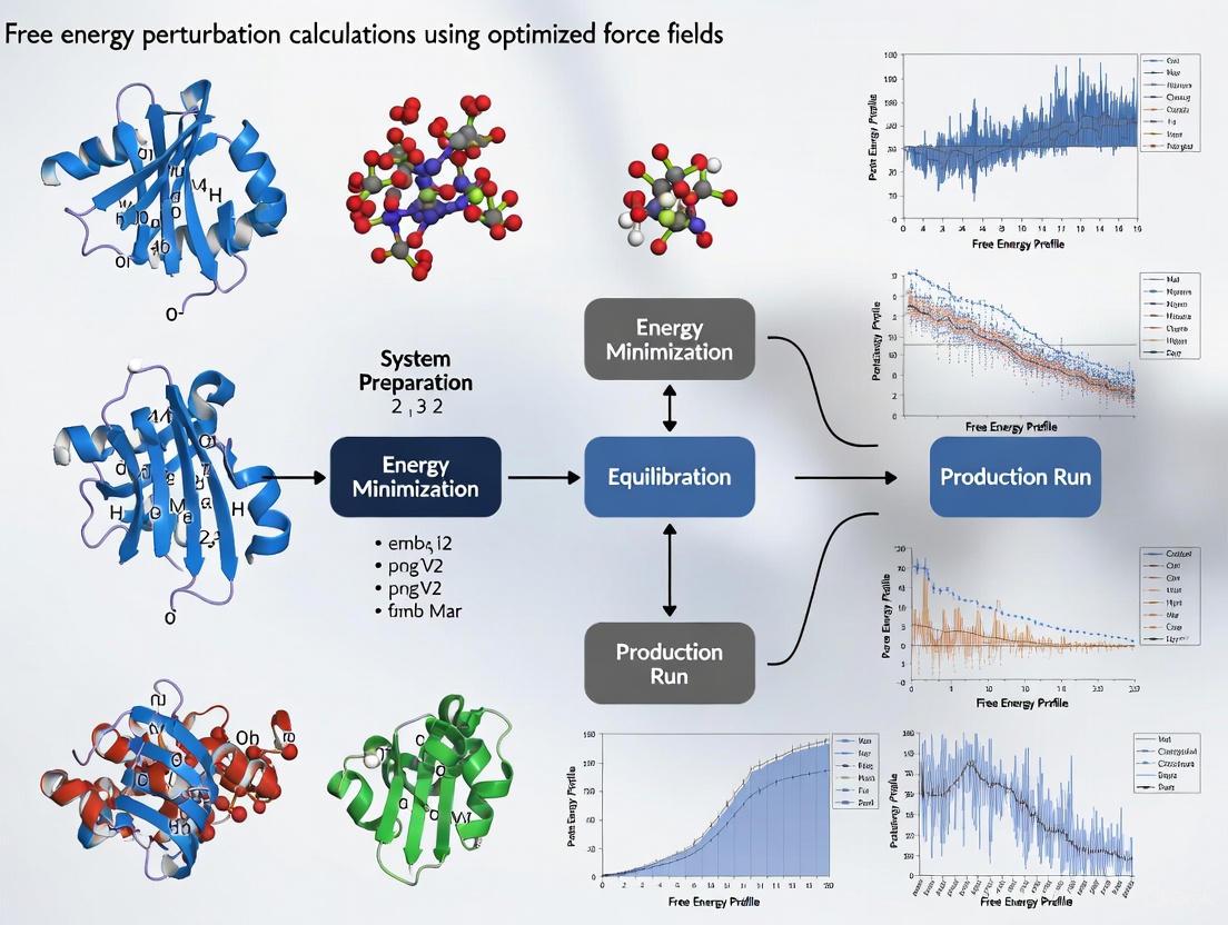
Free Energy Perturbation (FEP) has emerged as a pivotal tool in computational drug discovery, enabling researchers to predict binding affinities with accuracy sufficient to guide lead optimization [1]. The reliability of any FEP calculation is fundamentally dependent on a well-considered setup, with three components acting as critical pillars: the careful scheduling of lambda (λ) windows for the alchemical transformation, the selection of an appropriate Hamiltonian (the mathematical description of the system's energy), and the implementation of robust sampling protocols to adequately explore the system's conformational space [26] [27]. This application note details advanced methodologies and protocols for these key components, providing a framework for obtaining high-quality, predictive free energy results.

Core Components of an FEP Setup

Lambda Windows Scheduling and Pathway Selection

The alchemical transformation in FEP is achieved by dividing the pathway between the two end-states (e.g., ligand A and ligand B) into a series of intermediate λ windows, where λ typically ranges from 0 (initial state) to 1 (final state). The strategy for selecting the number and distribution of these windows, as well as the pathway of the transformation, is crucial for convergence and accuracy.

Table 1: Lambda Scheduling Strategies for Different Transformation Types

Transformation Type	Recommended Pathway	Key Lambda Parameters	Considerations
Small, Non-Polar Changes [28]	One-step (simultaneous VdW & electrostatics)	12-21 λ windows; uniform spacing often sufficient	Computationally most efficient; suitable for perturbations with high phase-space overlap.
Typical RBFE [29]	Two-step (electrostatics off, then VdW change)	21 λ windows; coul_lambdas: 1→0, then vdw_lambdas: 0→1	Prevents instabilities from atoms appearing/disappearing; standard for many perturbations.
Charge-Changing Perturbations [1] [29]	Three-step (elec off, VdW change, elec on)	~16 λ windows; independent coul_lambdas and vdw_lambdas for each leg	Manages charge interactions carefully; requires longer simulation times (~2x) for convergence [1].

A significant advancement in this area is the move away from user-guessed lambda counts towards automated lambda scheduling algorithms. These systems use short exploratory calculations to determine the optimal number of windows for each specific perturbation, thereby maximizing accuracy while conserving valuable GPU resources [1].

Hybrid Hamiltonians in FEP

The Hamiltonian, or the energy function describing the system, is central to the FEP calculation. The choice of force field and the potential integration of hybrid quantum mechanics/molecular mechanics (QM/MM) methods constitute the Hamiltonian's foundation.

Table 2: Comparison of Hamiltonian Descriptions for FEP

Hamiltonian Type	Description	Advantages	Challenges
Classical MM Force Fields [1] [28]	Uses molecular mechanics potentials (e.g., AMBER, CHARMM, OpenFF).	Fast, well-validated for standard residues, compatible with enhanced sampling.	Accuracy limited by force field parametrization; poor description of atypical ligands or electronic effects.
Polarizable Force Fields [30]	Includes many-body polarization effects (e.g., AMOEBA).	Superior treatment of electrostatics, crucial for RNA and highly charged systems.	Computationally more expensive; requires careful parameterization.
QM/MM Hybrid [31] [32]	QM treatment for ligand/key residues; MM for environment.	High accuracy for chemical reactions, halogen bonds, and charge transfer.	Significantly more computationally intensive; complex setup.

Modern implementations are making QM/MM FEP more accessible. Platforms like QUELO can automate the setup, allowing hundreds of atoms to be treated at the QM level during the simulation without manual intervention [31]. For systems where a full QM/MM treatment is prohibitive, a practical alternative is to use Quantum Mechanics (QM) calculations to refine specific force field parameters, such as torsion potentials, for ligands that are poorly described by the standard force field [1].

Enhanced Sampling Protocols

Adequate sampling of the conformational space is arguably the greatest challenge in FEP. Insufficient sampling leads to poor convergence and inaccurate free energy estimates. Enhanced sampling techniques are therefore essential.

Key Sampling Protocols:

• Replica Exchange with Solute Tempering (REST2): This widely adopted method enhances conformational sampling by simulating multiple replicas of the system at different "effective temperatures" applied only to the solute (e.g., the ligand and its immediate environment). This allows the system to overcome energy barriers that would otherwise trap it in a local minimum [26].
• Extended Pre-REST Sampling: Research has demonstrated that extending the equilibration or "pre-REST" sampling phase is critical, especially for flexible systems. The default pre-REST sampling (e.g., 0.24 ns/λ) is often insufficient. An improved protocol recommends:
  • 5 ns/λ pre-REST + 8 ns/λ REST: For systems with high-quality starting structures and no major conformational changes [26].
  • 2 × 10 ns/λ pre-REST: Two independent 10 ns/λ runs for systems undergoing significant structural rearrangements, helping to sample different energy minima [26].
• Lambda-Adaptive Biasing Force (λ-ABF): This state-of-the-art technique bypasses the need for discrete lambda windows altogether. It applies a continuous adaptive bias along the alchemical coordinate (λ), which drives the system to sample all intermediate states efficiently, often leading to faster convergence [30].
• Advanced Hydration Sampling: The treatment of water is critical. Techniques like Grand Canonical Monte Carlo (GCMC) can be integrated with MD to allow water molecules to be inserted and deleted from the binding site during the simulation, ensuring a proper hydration environment and reducing hysteresis [1].

Visualizing FEP Component Relationships and Workflow

The following diagrams illustrate the logical relationships between the core FEP components and a detailed experimental workflow.

Diagram 1: Interplay of core FEP components and their advanced implementations for tackling specific challenges.

Diagram 2: A detailed FEP setup and execution workflow, highlighting critical decision points and modern best practices.

The Scientist's Toolkit: Essential Research Reagents & Materials

Table 3: Key Software Tools and Force Fields for Advanced FEP

Tool / Resource	Type	Primary Function in FEP
AMBER [27]	MD Software Suite	Provides implementations of TI, FEP, and λ-dynamics, often used with the AMBER force fields.
Tinker-HP [30]	MD Software	GPU-accelerated package for performing simulations with polarizable force fields like AMOEBA.
Open Force Field (OpenFF) [1]	Force Field Initiative	Develops modern, accurate small molecule force fields (e.g., Parsley) for use in FEP simulations.
QUELO [31]	FEP Platform	Enables automated FEP setup and execution, including with AI-parametrized MM and QM/MM Hamiltonians.
GROMACS [29]	MD Software	Open-source package capable of running FEP calculations, offering high flexibility in lambda pathway setup.
ChemShell [32]	QM/MM Environment	Facilitates the setup and execution of complex QM/MM FEP calculations.
AMOEBA Force Field [30]	Polarizable Force Field	Provides a more physical description of electrostatics via induced atomic dipoles, critical for RNA and charged systems.

Detailed Experimental Protocol: An Improved FEP+ Sampling Protocol for Flexible Systems

This protocol is adapted from a study that systematically improved FEP accuracy for flexible ligand-binding domains [26].

Objective: To obtain precise ΔΔG predictions for a congeneric series of ligands binding to a protein target with a flexible binding site.

Required Inputs:

• A high-resolution protein structure (e.g., from X-ray crystallography).
• 3D structures of ligands in the series, with known experimental binding affinities for validation.
• Access to FEP-capable software (e.g., Schrödinger's FEP+, OpenFE, or similar).

Methodology:

• System Preparation:

  • Prepare the protein structure using standard tools (e.g., Protein Preparation Wizard). Add missing atoms, model missing loops, and optimize the hydrogen-bonding network.
  • Prepare ligand structures using LigPrep or similar, generating low-energy 3D conformations at the desired protonation state (pH 7.0 ± 2.0).
  • Critical Step: For each ligand, perform preliminary MD simulations (100-300 ns) of the ligand-protein complex. This identifies the correct binding mode, checks for system stability, and reveals flexible protein residues critical for binding.

• FEP Setup:

  • Align all ligands to a reference bound conformation based on the preliminary MD results and Maximum Common Substructure (MCS).
  • Define the perturbation map, connecting ligands with a maximum change of ~10 heavy atoms.
  • Define the pREST region: Based on the preliminary MD, include the entire ligand and important flexible protein residues from the binding site in the "hot" region for REST2 sampling [26].

• Simulation Execution:

  • Equilibration: Use the standard equilibration procedure provided by your software.
  • Sampling - Standard Flexibility Protocol:
    • Set the pre-REST sampling to 5 ns/λ.
    • Set the REST2 sampling to 8 ns/λ.
  • Sampling - High Flexibility Protocol (for significant backbone/loop motions):
    • Set the pre-REST sampling to 2 independent runs of 10 ns/λ.
    • Set the REST2 sampling to 8-10 ns/λ.

• Analysis:

  • Calculate the relative binding free energies (ΔΔG) using the Bennett Acceptance Ratio (BAR) or Multistate BAR (MBAR) method.
  • Check for hysteresis by comparing the forward and reverse transformations.
  • Validate the protocol by correlating calculated ΔΔG values with experimental data. The improved protocol should yield a higher correlation coefficient (R²) and a lower average absolute error (e.g., < 0.6 kcal/mol) compared to default settings [26].

The meticulous setup of an FEP calculation is a prerequisite for achieving predictive power in drug discovery projects. By moving beyond default parameters and adopting advanced strategies—such as automated lambda scheduling, polarizable or QM/MM Hamiltonians for challenging electronic environments, and rigorous sampling protocols like extended pre-REST and λ-ABF—researchers can reliably tackle increasingly complex biological targets, including protein-protein interactions and RNA riboswitches [1] [30]. The integration of these key components, as detailed in this application note, provides a robust foundation for advancing free energy calculations in structure-based drug design.

Advanced FEP Setups: From Standard Protocols to Cutting-Edge Integrations

Free Energy Perturbation (FEP) has emerged as a cornerstone technology in computational drug discovery, enabling researchers to predict protein-ligand binding affinities with accuracy approaching experimental methods [33]. The core principle of FEP involves computing the free energy difference between related compounds through alchemical transformations, providing invaluable insights for hit optimization and lead development [5] [1]. While the theoretical foundations of FEP are well-established, the practical implementation presents significant challenges, including the need for extensive computational resources, technical expertise in simulation setup, and careful parameter selection [5] [34]. Recent advances in workflow automation have begun to address these barriers, making rigorous free energy calculations more accessible to drug discovery teams.

The evolution of FEP methodologies has been marked by steady improvements in force field accuracy, enhanced sampling algorithms, and the development of more sophisticated workflow tools [1]. Modern FEP implementations can achieve predictive accuracies of approximately 1 kcal/mol, which is sufficient to guide medicinal chemistry decisions in lead optimization campaigns [33] [7]. This application note details protocols for implementing robust, automated FEP workflows using both commercial (Schrödinger's FEP+) and open-source (OpenMM) platforms, with emphasis on parameter optimization, validation strategies, and integration into drug discovery pipelines.

Quantitative Benchmarking of FEP Performance

The accuracy and reliability of FEP predictions are highly dependent on the choice of force fields, water models, and partial charge assignment methods. Based on comprehensive validation studies, the performance of different parameter combinations can be quantitatively compared to guide selection.

Table 1: Performance of Different Force Field Parameter Sets in FEP Calculations (AMBER/GAFF)

Parameter Set	Protein Forcefield	Water Model	Charge Model	MUE (kcal/mol)	RMSE (kcal/mol)	R²
1	AMBER ff14SB	SPC/E	AM1-BCC	0.89	1.15	0.53
2	AMBER ff14SB	TIP3P	AM1-BCC	0.82	1.06	0.57
3	AMBER ff14SB	TIP4P-EW	AM1-BCC	0.85	1.11	0.56
4	AMBER ff15ipq	SPC/E	AM1-BCC	0.85	1.07	0.58
5	AMBER ff14SB	TIP3P	RESP	1.03	1.32	0.45
FEP+ (OPLS2.1)	Custom OPLS2.1	SPC/E	CM1A-BCC	0.77	0.93	0.66

The benchmarking data reveals that parameter set 2 (AMBER ff14SB/TIP3P/AM1-BCC) achieves the best balance of low error and high correlation among the open-source combinations, with a mean unsigned error (MUE) of 0.82 kcal/mol and R² of 0.57 [5] [34]. The commercial FEP+ implementation with OPLS2.1 force field demonstrates superior overall performance (MUE = 0.77 kcal/mol, R² = 0.66), highlighting the impact of optimized force field parameters [5]. The RESP charge model consistently underperformed in these benchmarks, suggesting AM1-BCC provides more reliable partial charges for FEP applications.

Table 2: Comparison of FEP Platforms and Performance Characteristics

Platform	License	Force Fields	Key Features	Reported MUE (kcal/mol)	Primary Applications
FEP+	Commercial	OPLS4, OPLS5	GUI, REST2, Active Learning, FEP Protocol Builder	0.77-1.0 [5] [7]	Lead optimization, selectivity profiling, ADMET prediction
OpenMM/Alchaware	Open-source	AMBER, CHARMM, OpenFF	Customizable, Python API, extensive sampling methods	0.82-1.03 [5] [34]	Method development, custom simulations, academic research
OpenFE	Open-source	OpenFF, AMBER	Standardized workflows, interoperability	~1.0 (system dependent) [35]	Community-driven development, benchmarking

When considering experimental reproducibility as the fundamental limit of accuracy, recent studies have found that the reproducibility of relative binding affinity measurements between different experimental assays ranges from 0.77 to 0.95 kcal/mol [7]. This indicates that well-prepared FEP simulations can achieve accuracy comparable to experimental measurements, supporting their use in decision-making for drug discovery projects.

Automated Protocol Development with FEP Protocol Builder

The FEP Protocol Builder (FEP-PB) represents a significant advancement in automating the development of robust FEP protocols [36]. This active learning-based workflow addresses the challenge of systems that perform poorly with default FEP settings by iteratively searching the protocol parameter space to develop optimized FEP protocols with minimal human intervention.

Diagram 1: FEP Protocol Builder Active Learning Workflow. The automated process iteratively samples parameter space, runs FEP calculations, and updates machine learning models until convergence criteria are met.

The FEP-PB workflow begins with an initial protocol definition and target system input. The active learning loop then sequentially samples the parameter space, executes FEP calculations with error analysis, and updates the machine learning model to predict promising parameter combinations [36]. This cycle continues until predefined convergence criteria are met, outputting an optimized FEP protocol specifically tailored to the challenging system. This approach has been successfully demonstrated for previously problematic targets like MCL1 and p97, where default settings failed to produce predictive models [36].

Key parameters optimized by FEP-PB include:

• Sampling parameters: Simulation length, number of lambda windows, replica exchange settings
• Force field selection: Choice between OPLS4 and OPLS5 force fields [37]
• System-specific settings: Solvent and complex hot atom rules, REST region definitions
• Technical parameters: Integration timesteps, constraint algorithms, nonbonded treatment

The implementation of FEP-PB has demonstrated remarkable efficiency, reducing protocol development time from weeks or months of manual optimization to a fully automated process completing within days [36]. This acceleration makes FEP applicable to targets that were previously considered intractable, significantly expanding the domain of applicability of free energy calculations in drug discovery.

Open-Source FEP Implementation with OpenMM

For research environments requiring customization and flexibility, open-source tools like OpenMM provide a powerful platform for implementing automated FEP workflows. The OpenMM ecosystem offers extensive control over simulation parameters, force field implementations, and sampling algorithms.

Workflow Implementation

A robust open-source FEP workflow can be constructed using several interconnected components:

Diagram 2: Open-Source FEP Workflow with OpenMM. The process begins with structure preparation and proceeds through ligand posing, parameterization, simulation, and free energy analysis.

The OpenMM FEP workflow begins with careful preparation of protein-ligand complex structures. For congeneric series with common cores, the FEgrow tool can generate initial binding poses for novel analogs by enumerating and optimizing the bioactive conformations of grown functional groups [38]. FEgrow employs a hybrid machine learning/molecular mechanics (ML/MM) approach for conformer optimization and can score poses using the gnina convolutional neural network scoring function before proceeding to full free energy calculations [38].

Simulation Protocol

The production FEP simulation protocol in OpenMM should include the following key steps [5] [34]:

• System Setup:

  • Protein: AMBER ff14SB or ff15ipq force field
  • Ligands: GAFF2.11 with AM1-BCC partial charges
  • Solvent: TIP3P or SPC/E water models in an appropriate periodic box
  • Ions: Neutralization and physiological concentration (e.g., 150mM NaCl)

• Simulation Parameters:

  • Integration: 4fs timestep with hydrogen mass repartitioning
  • Temperature: 300K maintained with Langevin integrator
  • Pressure: 1 atm maintained with Monte Carlo barostat
  • Nonbonded interactions: Particle Mesh Ewald for electrostatics with 9Å cutoff

• FEP-Specific Settings:

  • Lambda windows: 12 equally-spaced windows for transformation
  • Enhanced sampling: Hamiltonian replica exchange with solute tempering (REST)
  • Simulation length: 5-20ns production per window depending on system complexity
  • Convergence monitoring: Overlap statistics and hysteresis analysis

• Free Energy Analysis:

  • Free energy estimator: Multistate Bennett Acceptance Ratio (MBAR)
  • Error analysis: Block averaging or bootstrap confidence intervals
  • Validation: Cycle closure analysis for perturbation networks

This protocol, when implemented with parameter set 2 (AMBER ff14SB/TIP3P/AM1-BCC), has demonstrated robust performance across eight benchmark test cases (BACE, CDK2, JNK1, MCL1, P38, PTP1B, Thrombin, and TYK2) with diverse chemical transformations [5] [34].

The Scientist's Toolkit: Essential Research Reagents and Solutions

Successful implementation of automated FEP workflows requires both software tools and methodological components. The following table details essential "research reagents" for establishing robust FEP protocols.

Table 3: Essential Research Reagents for Automated FEP Workflows

Tool/Component	Type	Function	Implementation Examples
Force Fields	Parameter set	Describes molecular interactions and energetics	OPLS4/OPLS5 (FEP+), AMBER ff14SB/ff15ipq (OpenMM), GAFF2.11 (ligands) [5] [37]
Water Models	Solvent parameter	Represents aqueous environment and solvation effects	SPC/E, TIP3P, TIP4P-EW [5] [34]
Partial Charge Methods	Electronic parameter	Calculates atomic partial charges for electrostatics	AM1-BCC, RESP, CM1A-BCC [5] [34]
Enhanced Sampling	Algorithm	Improves conformational sampling efficiency	REST2 (FEP+), Hamiltonian RE (OpenMM) [5]
Ligand Pose Generator	Software tool	Generates initial binding poses for novel analogs	FEgrow (open-source), Core-constrained docking [38]
Free Energy Estimator	Analysis algorithm	Calculates free energies from simulation data	MBAR, TI, Bennett Acceptance Ratio [5] [34]
Protocol Optimizer	Automation tool	Automates FEP parameter optimization	FEP Protocol Builder (FEP+), Active Learning [36]
Validation Benchmarks	Dataset	Validates protocol accuracy and performance	JACS set, internal project data [5] [35]

Advanced Applications and Future Directions

The application of automated FEP workflows has expanded significantly beyond traditional R-group optimization in lead optimization. Current advanced applications include:

Absolute Binding FEP (ABFE): Unlike relative FEP, which calculates binding energy differences between similar compounds, ABFE computes the absolute binding free energy of individual ligands without requiring a reference compound [1]. This approach is particularly valuable for virtual screening applications where diverse chemotypes need evaluation. While computationally more expensive (approximately 10× RBFE), ABFE offers greater flexibility in chemical space exploration and can utilize different protein structures optimized for specific ligands [1].

Membrane Protein Targets: Automated FEP workflows have been successfully extended to challenging membrane protein systems such as GPCRs and ion channels [1]. These implementations require careful handling of membrane bilayers, with potential system truncation strategies to maintain computational efficiency without sacrificing accuracy [1].

Active Learning for Large-Scale Screening: The integration of FEP with active learning frameworks enables efficient screening of massive compound libraries (up to millions of compounds) [33] [1]. In this approach, a machine learning model is trained on initial FEP data and used to prioritize compounds for subsequent FEP calculations, creating an iterative cycle of prediction and validation that maximizes the information gain per computational cost [33].

Covalent Inhibitors and Alternative Modalities: Recent methodology developments have addressed the challenges of modeling covalent inhibitors, where specialized parameters are needed to describe the bond formation between ligand and protein [1]. Similarly, FEP workflows are being adapted for bifunctional degraders (PROTACs) and other complex modalities that require multi-component binding simulations [37].

As FEP methodologies continue to evolve, we anticipate further automation, improved accuracy through better force fields and sampling, and expanded applicability to increasingly complex biological systems and therapeutic modalities.

Machine Learning Force Fields (MLFFs) represent a paradigm shift in computational atomistic simulations, offering a pathway to achieve quantum-mechanical accuracy at a fraction of the computational cost of traditional ab initio methods. The fundamental challenge in molecular modeling has historically been the trade-off between accuracy and computational efficiency. While Density Functional Theory (DFT) provides reasonable accuracy for many chemical systems, its computational expense fundamentally limits the time- and length-scales accessible for simulation. Conversely, classical force fields, though computationally efficient, often lack the accuracy and transferability required for predicting complex chemical properties due to their simplified functional forms. MLFFs bridge this critical gap by leveraging machine learning algorithms to infer complex potential energy surfaces (PES) from reference quantum mechanical calculations, enabling accurate molecular dynamics (MD) simulations of large systems over meaningful timescales.

The theoretical foundation of MLFFs rests on their ability to approximate the Born-Oppenheimer PES through flexible, data-driven models. Unlike traditional force fields that use fixed mathematical forms with empirically parameterized terms, MLFFs employ high-capacity function approximators—such as neural networks or kernel methods—that learn the relationship between atomic configurations and energies/forces from reference data. This approach allows MLFFs to capture many-body interactions, chemical reactivity, and complex bonding environments with unprecedented fidelity. Recent architectural innovations, such as message passing networks and equivariant models, have further enhanced their capabilities by efficiently handling diverse chemical elements and long-range interactions. The resulting force fields achieve accuracy close to their quantum mechanical reference methods while enabling molecular dynamics simulations that are several orders of magnitude faster than direct ab initio MD.

MLFFs for Free Energy Calculations

Free energy perturbation (FEP) calculations represent a cornerstone of computational drug discovery, particularly in predicting relative binding affinities for ligand optimization. Traditional FEP approaches relying on classical force fields face fundamental accuracy limitations due to their simplified functional forms which cannot quantitatively reproduce ab initio methods without significant parameter tuning. MLFFs offer a transformative solution to this challenge by retaining quantum mechanical accuracy while maintaining sufficient computational efficiency for the extensive sampling required in free energy calculations.

A groundbreaking demonstration of this capability comes from a recent workflow that combines a broadly trained MLFF, termed Organic_MPNICE, with enhanced sampling techniques for calculating hydration free energies (HFEs) of diverse organic molecules. This approach achieved sub-kcal/mol average errors relative to experimental values—surpassing the accuracy of state-of-the-art classical force fields and DFT-based implicit solvation models. The critical advancement lies in the integration of MLFFs with sufficient statistical and conformational sampling empowered by solute-tempering techniques, establishing a robust pathway to ab initio-quality free energy predictions for drug discovery applications. This methodological breakthrough demonstrates that MLFFs can successfully address the accuracy limitations that have long plagued classical force fields in FEP calculations, particularly for systems where electronic effects, polarization, and precise bonding interactions play crucial roles in determining binding affinities.

Table 1: Performance Comparison of Free Energy Calculation Methods

Method Type	Representative Example	Average HFE Error (kcal/mol)	Key Limitations
Classical Force Fields	State-of-the-art parametrized FF	>1.0	Simplified functional forms, limited transferability
DFT-based Implicit Solvation	Various implicit models	>1.0	Inaccurate treatment of explicit solvent effects
MLFF-based Approach	Organic_MPNICE with solute-tempering	<1.0	Higher computational cost than classical FF

Experimental Protocols and Application Notes

Automated Training Protocol for Catalytic Barrier Accuracy

The accuracy of MLFFs in predicting energy barriers is crucial for modeling chemical reactions, including those relevant to drug metabolism and enzymatic processes. A robust training protocol has been developed specifically for generating MLFFs capable of determining energy barriers within 0.05 eV of DFT reference values. This protocol employs active learning (AL) to automate the collection of training data, systematically improving the model's accuracy in relevant regions of the potential energy surface without prior knowledge of reaction path energetics.

The protocol consists of six sequential active learning blocks that progressively refine the MLFF. The initial blocks model the surface itself through molecular dynamics with uncertainty-based sampling, where configurations are selected for DFT calculation when the local energy uncertainty of any atom exceeds a predefined threshold (typically 50 meV). Subsequent blocks focus on geometry optimization and nudged elastic band (NEB) calculations to accurately capture adsorption energies and barriers. This structured approach ensures comprehensive sampling of the configuration space while minimizing the number of expensive DFT calculations required. The protocol's effectiveness has been validated on the hydrogenation of carbon dioxide to methanol over indium oxide, with the resulting MLFF not only reproducing established barriers but also discovering an alternative reaction path with a 40% reduction in activation energy—demonstrating how MLFFs can enhance our understanding of even extensively studied systems.

Hydration Free Energy Calculation Protocol

For drug discovery applications, calculating hydration free energies with quantum accuracy requires a specialized protocol leveraging MLFFs:

• System Preparation: Construct initial configurations for organic molecules solvated in explicit water boxes, ensuring sufficient solvent shell thickness to minimize periodic boundary artifacts.

• MLFF Selection and Validation: Employ a broadly trained MLFF such as Organic_MPNICE that incorporates long-range interactions and charge equilibration. Validate force field accuracy on known benchmark molecules before proceeding to unknown systems.

• Enhanced Sampling Configuration: Implement solute-tempering techniques to improve phase space sampling. Configure Hamiltonian replica exchange with specific focus on scaling interactions between the solute and surrounding solvent molecules.

• Equilibration Phase: Perform extensive equilibration using MLFF-MD simulations, monitoring key thermodynamic properties and convergence metrics to ensure system stability.

• Production Simulation: Conduct multi-nanosecond MLFF-MD simulations, saving trajectories at regular intervals for subsequent analysis. The computational efficiency of MLFFs enables longer sampling times than possible with direct ab initio MD.

• Free Energy Extraction: Calculate HFEs using thermodynamic integration or free energy perturbation methods applied to the MLFF-MD trajectories. Employ bootstrapping analysis to estimate statistical uncertainties.

This protocol has demonstrated sub-kcal/mol accuracy across a diverse set of 59 organic molecules, establishing a new benchmark for ab initio-quality hydration free energy predictions.

Active Learning Integration with Foundational Models

The development of accurate MLFFs benefits significantly from integration with active learning frameworks and foundational models. The aims-PAX (Parallel Active eXploration) platform exemplifies this approach, providing an automated, multi-trajectory active learning workflow that streamlines MLFF development. This framework combines flexible sampling with scalable training across CPU and GPU architectures, offering several key advantages:

Initial dataset generation can be dramatically accelerated using general-purpose MLFFs as geometry generators, which produce physically plausible system geometries that are subsequently recomputed using reference ab initio methods. This approach decorrelates geometries and improves computational efficiency by at least an order of magnitude compared to traditional ab initio MD sampling. The active learning loop then iteratively identifies configurations where the MLFF exhibits high uncertainty, selects these for DFT verification, and retrains the model on the expanded dataset. This process continues until the MLFF achieves target accuracy across all relevant regions of the configuration space, as measured by uncertainty metrics and validation against known benchmarks.

Table 2: Essential Research Reagent Solutions for MLFF Implementation

Resource Category	Specific Examples	Function in MLFF Workflow
MLFF Architectures	MACE, MPNICE, NequIP	Core model architectures for learning atomic potentials
Active Learning Platforms	aims-PAX, FLARE, ALF	Automated data selection and model improvement
Reference Electronic Structure Codes	FHI-aims, VASP, CASTEP	Generation of training data with quantum accuracy
General-Purpose Foundational Models	MACE-MP0, Organic_MPNICE	Starting points for transfer learning and system initialization
Enhanced Sampling Tools	PLUMED, ASE	Managing biased simulations for free energy calculations

Visualization of Workflows

MLFF Development via Active Learning

FEP Calculation with MLFFs

Performance Benchmarks and Applications

Quantitative Performance Assessment

The transformative potential of MLFFs is best demonstrated through quantitative benchmarks against established computational methods. In free energy calculations, the Organic_MPNICE model achieves remarkable accuracy, with average errors in hydration free energy predictions below 1 kcal/mol for diverse organic molecules—surpassing the accuracy of both state-of-the-art classical force fields and DFT-based implicit solvation models. This sub-kcal/mol accuracy is particularly significant as it approaches the threshold required for reliable prediction of binding affinities in drug discovery applications.

Beyond free energy calculations, MLFFs have demonstrated exceptional performance across multiple domains. In catalytic applications, specialized MLFFs achieve energy barrier predictions within 0.05 eV of DFT references while reducing the computational cost of routine in-silico catalytic tasks by orders of magnitude. For material property predictions, MLFFs enable high-throughput screening of 10⁷ to 10⁸ crystal structures, leading to the identification of promising Li-ion and Na-ion solid electrolytes. The computational speedup afforded by MLFFs not only reduces the cost of established simulation protocols but also enables previously intractable investigations, such as discovering alternative reaction pathways with significantly reduced activation energies and computing free energy barriers that account for finite-temperature effects.

Emerging Applications in Electrochemistry and Drug Discovery

MLFFs are finding increasingly diverse applications across electrochemical systems and drug discovery pipelines. In electrochemistry, MLFFs enable all-atom molecular dynamics simulations for accurate evaluation of ionic conductivity via the fluctuation-dissipation theorem and nonequilibrium MD under electric fields, applied to both solid and polymer electrolytes. For electrochemical reactions, MLFFs and Δ-ML models successfully predict redox potentials in homogeneous and interfacial systems through thermodynamic integration. These capabilities are particularly valuable for designing next-generation battery systems and electrocatalysts, where complex interfacial phenomena and reaction kinetics determine device performance.

In pharmaceutical applications, MLFFs facilitate the extraction of key thermodynamic and kinetic information—such as free energy landscapes and local transport coefficients—from atomic trajectories, enabling coarse-grained modeling of mass transport and reactions in complex biological environments. This multi-scale approach bridges the gap between quantum-accurate simulations and biologically relevant timescales, offering new insights into drug-receptor interactions, solvation effects, and metabolic transformation pathways. The integration of MLFFs with enhanced sampling methods further accelerates the exploration of conformational landscapes and binding modes, potentially reducing the empirical screening burden in early drug discovery.

Table 3: MLFF Performance Across Application Domains

Application Domain	Key Metric	MLFF Performance	Reference Method Performance
Hydration Free Energy	Mean Absolute Error (kcal/mol)	<1.0	>1.0 (Classical FF)
Catalytic Energy Barriers	Deviation from DFT (eV)	<0.05	N/A (DFT reference)
Ionic Conductivity	Accuracy vs. Experiment	Quantitative prediction	Limited by empirical parameterization
Reaction Pathway Discovery	Barrier Reduction	Up to 40%	Limited by manual sampling

Molecular dynamics (MD) simulations are indispensable for studying biological processes at atomic resolution, but their utility is often limited by the need for adequate sampling of conformational states. Enhanced sampling techniques, particularly Hamiltonian Replica Exchange Molecular Dynamics (H-REMD) and its variant Replica Exchange with Solute Tempering 2 (REST2), have emerged as powerful methods to overcome energy barriers and accelerate convergence in free energy calculations. This application note details the theoretical foundations, practical protocols, and key applications of these methods in the context of modern drug discovery, providing researchers with actionable methodologies for implementing these techniques in free energy perturbation calculations with optimized force fields.

Comprehensive sampling of biomolecular conformational space remains a significant challenge in computational chemistry and drug discovery due to the high energy barriers separating local minima, leading to kinetic trapping and quasi-ergodicity in simulations [39]. Generalized ensemble algorithms, particularly replica exchange methods, have been developed to facilitate more effective exploration of conformational landscapes by inducing random walks in parameter spaces.

The Replica Exchange Method (REM), originally introduced by Sugita and Okamoto, involves simulating multiple non-interacting copies (replicas) of a system at different temperatures, with periodic attempts to exchange configurations between adjacent temperatures [40]. This approach enables conformations to escape local energy minima through higher thermal fluctuations. However, the number of replicas required for efficient sampling in traditional Temperature REM (TREM) scales with the square root of the system's total degrees of freedom, making it computationally prohibitive for large solvated biomolecular systems [39].

Hamiltonian Replica Exchange Molecular Dynamics (H-REMD) addresses this limitation by maintaining all replicas at the same physical temperature but evolving them under different potential energy functions [41]. The differing Hamiltonians are typically created through alchemical transformations or selective scaling of energy terms, significantly reducing the number of replicas required compared to TREM. H-REMD has been successfully applied to diverse challenges including alchemical free energy calculations, protein folding, and characterization of intrinsically disordered proteins [42] [41].

Replica Exchange with Solute Tempering (REST) and its improved variant REST2 represent specialized implementations of H-REMD where enhanced sampling is focused specifically on the solute degrees of freedom [39]. In REST2, the potential energy function for replica m is defined as:

[ Em^{REST2}(X) = \frac{\betam}{\beta0}E{pp}(X) + \sqrt{\frac{\betam}{\beta0}}E{pw}(X) + E{ww}(X) ]

where (E{pp}), (E{pw}), and (E{ww}) represent protein-protein, protein-water, and water-water interaction energies, respectively; (\betam = 1/kBTm) and (\beta0 = 1/kBT_0) [39]. This scaling reduces energy barriers in the solute's intramolecular potential while maintaining the solvent at realistic conditions, dramatically improving sampling efficiency for biomolecular systems in explicit solvent.

Key Methodological Components

REST2 Energy Scaling and Parameterization

The REST2 method employs a specific scaling protocol that differentially affects various energy components of the system. The scaling factors applied to different interaction types are summarized in Table 1.

Table 1: REST2 Energy Scaling Parameters

Energy Component	Scaling Factor	Practical Implementation
Solute intramolecular ((E_{pp}))	(\betam/\beta0)	Scale dihedral force constants; bond and angle terms typically left unscaled
Solute-solvent ((E_{pw}))	(\sqrt{\betam/\beta0})	Scale solute atom charges and Lennard-Jones ε parameters
Solvent-solvent ((E_{ww}))	1 (unscaled)	No modification of water parameters

This selective scaling strategy effectively creates a "hot solute" in "cold solvent" environment, focusing computational resources on sampling the relevant biomolecular degrees of freedom while maintaining a realistic solvent environment [39]. The acceptance probability for replica exchange between replicas m and n in REST2 is determined by:

[ \Delta{mn}^{REST2} = (\betam - \betan)\left[(E{pp}(Xn) - E{pp}(Xm)) + \frac{\beta0}{\betam + \betan}(E{pw}(Xn) - E{pw}(Xm))\right] ]

The improved performance of REST2 over its predecessor (REST1) stems from two key modifications: (1) the scaling factor for protein-water interactions is changed from ((\beta0 + \betam)/2\betam) to (\sqrt{\betam/\beta0}), and (2) the approximate cancellation of (E{pp}) and the scaled (E_{pw}) in the acceptance probability, which enhances exchange rates between replicas [39].

Replica Exchange Process and Workflow

The replica exchange methodology follows a well-defined workflow that alternates between molecular dynamics propagation and configuration exchange attempts. The following diagram illustrates this process and the energy relationships in REST2:

Diagram 1: REST2 Workflow and Energy Scaling. The process involves parallel MD propagation with periodic exchange attempts between adjacent replicas, with energy terms scaled differently according to the REST2 protocol.

Application Protocols

Protocol 1: REST2 for Protein Folding and Conformational Sampling

Application: Enhanced sampling of protein conformational landscapes, particularly for systems with large-scale structural changes such as folding/unfolding transitions or intrinsically disordered proteins (IDPs).

System Preparation:

• Force Field Selection: Utilize recently optimized force fields such as Amber ff03ws with TIP4P/2005s or Amber ff99SB-disp with modified TIP4P-D for IDPs [42].
• Solvation: Employ explicit solvent models with appropriate ion concentrations to maintain physiological ionic strength.
• Replica Parameters: Determine optimal temperature distribution with 8-16 replicas covering effective solute temperatures from 300K to 500K, with exponential spacing.

Simulation Parameters:

• Integration: Use a timestep of 2 fs with constraints on bonds involving hydrogen atoms.
• Electrostatics: Employ Particle Mesh Ewald (PME) for long-range electrostatics with a real-space cutoff of 9-10 Å.
• Exchange Attempts: Attempt replica exchanges every 1-2 ps to maintain high acceptance rates (target 20-30%).
• Simulation Length: Conduct simulations of 500 ns per replica for systems up to 100 residues; extend to 1 μs per replica for larger systems [42].

Analysis:

• Monitor convergence through radius of gyration, secondary structure content, and native contacts.
• Calculate theoretical Small-Angle X-ray Scattering (SAXS) profiles and compare with experimental data where available [42].
• Assess sampling quality by comparing forward and backward transitions between conformational states.

Protocol 2: H-REMD for Alchemical Free Energy Calculations

Application: Calculation of relative binding free energies for drug discovery applications, particularly congeneric series of small molecules binding to protein targets.

System Preparation:

• Ligand Parameterization: Generate high-quality force field parameters for all ligands using appropriate tools (e.g., GAFF2 with AM1-BCC charges).
• Ligand Alignment: Ensure proper structural alignment of ligands in binding site to minimize unnecessary perturbations during alchemical transformations.
• λ Schedule: Define 16-24 λ windows with closer spacing near end states (λ = 0, 1) where nonlinearities in the free energy profile are expected.

Simulation Parameters:

• Sampling Method: Utilize the Replica Exchange Free Energy Perturbation (REFEP) approach, which combines H-REMD with FEP [41].
• Soft-Core Potentials: Implement soft-core potentials for Lennard-Jones and electrostatic interactions to avoid singularities.
• Enhanced Sampling: Apply dihedral angle biasing or other orthogonal sampling enhancements to improve side-chain rearrangements [41].
• Convergence Monitoring: Calculate free energy differences using both forward and backward transformations and monitor the hysteresis between them.

Analysis:

• Compute free energy differences using Multistate Bennett Acceptance Ratio (MBAR) or similar analysis techniques.
• Validate predictions against experimental binding affinities and assess statistical uncertainty through bootstrapping or block averaging.
• For prospective drug design, aim for accuracy comparable to experimental reproducibility (approximately 0.5-1.0 kcal/mol) [7].

Protocol 3: REST2 for Intrinsically Disordered Proteins

Application: Generation of unbiased structural ensembles of intrinsically disordered proteins (IDPs) for comparison with ensemble-averaged experimental data.

System Preparation:

• Initial Extended Structures: Start from fully extended conformations to avoid bias toward folded states.
• Enhanced Water Models: Use water models specifically optimized for IDP simulations (TIP4P-D or TIP4P/2005s) [42].
• Replica Setup: Implement 12-16 replicas with effective temperature range of 300-500K, focusing scaling on protein dihedral angles and nonbonded interactions.

Simulation Parameters:

• Simulation Length: Conduct 500 ns per replica for IDPs up to 100 residues; longer simulations for larger systems [42].
• Exchange Frequency: Attempt exchanges every 1-2 ps to maintain adequate mixing.
• Restart Capability: Implement checkpointing to enable extended sampling as needed.

Validation:

• Calculate theoretical SAXS/SANS profiles and compare with experimental data using χ² metrics [42].
• Compute NMR chemical shifts and compare with experimental values.
• Analyze polymer properties including persistence length and scaling exponents to characterize chain statistics.

Performance and Validation

Quantitative Performance Assessment

The performance of REST2 and H-REMD has been rigorously evaluated across multiple biological systems. Table 2 summarizes key performance metrics from published studies.

Table 2: Performance Metrics for REST2 and H-REMD Across Various Systems

System	Method	Performance Gain	Key Result	Reference
Trpcage and β-hairpin	REST2 vs TREM	3-5x reduction in replicas	Improved sampling of folded/unfolded states	[39]
Thioredoxin (pKa prediction)	H-REMD/FEP	Faster convergence vs TI and FEP	pKa accuracy within 0.4 units of experiment	[41]
Intrinsically Disordered Proteins	HREMD vs standard MD	Quantitative agreement with SAXS/SANS	Unbiased ensembles without reweighting	[42]
Protein-ligand binding	FEP+ with REST	Accuracy comparable to experimental reproducibility	~0.5-1.0 kcal/mol error	[7]

REST2 has demonstrated particular effectiveness for systems undergoing large conformational changes. In applications to trpcage and β-hairpin folding, REST2 showed significantly improved sampling efficiency compared to both TREM and the original REST formulation, with enhanced exchange between folded and extended conformations [39]. This improvement stems from both the modified scaling of the protein-water interaction term and the effective reduction of energy barriers in the scaled replicas.

For intrinsically disordered proteins, HREMD has proven essential for generating accurate structural ensembles. Recent studies have shown that while standard MD simulations can reproduce local experimental observables such as NMR chemical shifts, they often fail to capture global properties derived from small-angle scattering [42]. In contrast, HREMD-generated ensembles simultaneously agree with both local and global experimental measurements, providing unbiased representations of IDP structural distributions.

In drug discovery applications, free energy calculations enhanced by replica exchange methods have achieved accuracy comparable to experimental reproducibility. Comprehensive assessments have found that careful application of these methods can predict relative binding affinities with errors of approximately 0.5-1.0 kcal/mol, matching the reproducibility of typical experimental measurements [7].

Validation Against Experimental Data

Robust validation of enhanced sampling methods requires comparison with multiple experimental techniques:

Small-Angle Scattering: Calculate theoretical SAXS and SANS profiles from simulation trajectories and compare with experimental data using χ² metrics. HREMD consistently outperforms standard MD in reproducing scattering profiles for IDPs [42].

NMR Spectroscopy: Compute chemical shifts from simulation ensembles and compare with experimental values. Both standard MD and HREMD can reproduce chemical shifts, suggesting they are insufficient as sole validation metrics [42].

Binding Affinities: For drug discovery applications, validate computed relative binding free energies against experimentally measured affinities from isothermal titration calorimetry (ITC) or inhibition assays.

Research Toolkit

Essential Software and Force Fields

Table 3: Research Reagent Solutions for Enhanced Sampling Simulations

Tool Category	Specific Solutions	Function	Application Context
Force Fields	Amber ff03ws, Amber ff99SB-disp	Protein force fields optimized with IDP and water model adjustments	IDP simulations with explicit solvent [42]
Water Models	TIP4P-D, TIP4P/2005s	Water models specifically parameterized for disordered proteins	Accurate solvation of IDPs and folded proteins [42]
Enhanced Sampling Packages	REST2 implementations in GROMACS, AMBER	Specialized scaling of solute Hamiltonian components	Protein folding and conformational sampling [39]
Free Energy Tools	FEP+, alchemical analysis tools	Automated setup and analysis of free energy calculations	Drug discovery and binding affinity prediction [7]
Analysis Software	WHAM, MBAR, variational FEP	Free energy estimation from replica exchange simulations	Post-processing of enhanced sampling data [27]

Best Practices for Implementation

Replica Setup Optimization:

• Determine replica spacing to maintain exchange acceptance rates of 20-30%.
• For REST2, focus scaling primarily on dihedral terms and nonbonded interactions.
• Use tools such as temperature predictor utilities to optimize replica distributions.

Convergence Assessment:

• Monitor forward and backward transitions between conformational states.
• Calculate statistical uncertainties through block analysis or bootstrapping.
• Compare multiple independent simulations to assess reproducibility.

Force Field Selection:

• Choose force fields specifically optimized for the system of interest (e.g., IDP-optimized potentials for disordered proteins).
• Validate force field performance against available experimental data before large-scale production simulations.

Replica Exchange with Solute Tempering (REST2) and Hamiltonian Replica Exchange Molecular Dynamics represent powerful enhancements to standard molecular dynamics simulations, enabling comprehensive sampling of biomolecular conformational landscapes that would otherwise be computationally prohibitive. When properly implemented with optimized force fields and validated against experimental data, these methods provide robust platforms for addressing challenging problems in structural biology and drug discovery, from characterizing intrinsically disordered proteins to predicting ligand binding affinities with accuracy approaching experimental reproducibility. The protocols outlined in this application note provide researchers with practical guidance for implementing these advanced sampling techniques in their computational studies.

Nonequilibrium Switching (NES) represents a paradigm shift in the calculation of relative binding free energy (RBFE), a critical parameter for predicting the binding affinity of potential drug molecules in lead optimization. Traditional alchemical methods, such as Free Energy Perturbation (FEP) and Thermodynamic Integration (TI), rely on simulating a gradual transformation from one ligand to another through a series of intermediate states, each requiring extensive simulation to reach thermodynamic equilibrium. This process is computationally expensive, often taking hours on powerful hardware for each transformation. In contrast, NES utilizes many short, bidirectional, and independent switching simulations that drive the system far from equilibrium. Grounded in the statistical physics formalized by Jarzynski, the NES approach collectively uses the statistics from these rapid transitions to yield accurate free energy differences, achieving a 5-10X higher throughput than conventional equilibrium methods [43] [6].

The core application of NES is the prediction of Relative Binding Free Energy (RBFE), denoted as ΔΔG. This value quantifies the difference in binding affinity between two similar ligands, A and B, to a target protein (ΔΔG = ΔG_B - ΔG_A). Instead of computing the absolute binding affinities directly, a thermodynamic cycle is employed, requiring the calculation of two alchemical transformations: the mutation of ligand A to B in the protein's binding site (ΔG_Bound) and in solution (ΔG_Unbound). The relative binding affinity is then given by ΔΔG = ΔG_Bound - ΔG_Unbound [44].

Application Notes: Performance and Advantages

Quantitative Performance and Benchmarking

Industry benchmarks demonstrate that NES provides market-leading accuracy comparable to traditional FEP and TI methods, but with dramatically improved speed and cost-effectiveness. Scientists report that for a set of 40 ligands, calculations that would take 24-36 hours with FEP+ can be completed in just 2-3 hours using NES on cloud platforms like Orion [6]. This performance makes large-scale RBFE calculations feasible within the timelines of active drug discovery projects.

Table 1: Comparative Performance of NES vs. Traditional Equilibrium Methods

Feature	Traditional FEP/TI	Nonequilibrium Switching (NES)
Throughput	Lower (reference)	5-10X higher [43]
Typical Compute Time for 40 ligands	24-36 hours [6]	2-3 hours [6]
Simulation Paradigm	Series of dependent equilibrium states	Swarms of independent, fast transitions
Sampling Efficiency	Slower, requires equilibrium at each state	Efficiently navigates complex energy landscapes [43]
Scalability & Resilience	Moderate, due to sequential dependencies	Highly parallel and fault-tolerant [43]

Validation on public benchmark datasets, such as Schindler (2020) and Wang (2015), shows that NES delivers accuracy with no significant aggregate performance differences compared to equilibrium methods. This reliability, combined with its speed, makes NES a powerful tool for guiding lead optimization [6].

Key Advantages in Drug Discovery Workflows

• High Throughput and Fast Feedback: The short duration of NES switches (tens to hundreds of picoseconds) means partial results are available quickly. This enables adaptive workflows where computational resources can be reallocated to the most promising compounds in near real-time [43].
• Unparalleled Scalability and Resilience: Each switching simulation is independent, making the method "embarrassingly parallel." This architecture is ideal for modern cloud computing frameworks, where thousands of simulations can be run simultaneously. The failure of individual runs does not compromise the overall calculation, as the collective statistics from the remaining successful runs remain valid [43] [44].
• Handling of Complex Transformations: NES has been shown to support alchemical changes between ligands with different formal charges, a challenging scenario for some free energy methods [6]. Furthermore, its performance can be enhanced for flexible binding sites by integrating with methods like Induced-Fit Posing (IFP) [6].

Detailed Experimental Protocol

The following protocol is adapted from automated workflows, such as the Equilibration and Nonequilibrium Switching Floe available on the Orion platform [44].

System Preparation and Equilibration

• Protein and Ligand Preparation:

  • Protein Input: The target protein must be prepared to "MD-ready" standards. This includes adding all missing atoms (including hydrogens), assigning correct protonation and tautomeric states for side chains, capping chain termini, and resolving missing loops. The use of a tool like Spruce is strongly recommended. The input file can be provided separately or embedded within the ligand dataset as a Spruce design unit [44].
  • Ligand Input: Ligands must have reasonable 3D coordinates, all atoms, and correct chemistry, including bond orders and formal charges. Bad clashes with the protein should be relaxed prior to the simulation.
  • Edge Mapping: A ligand mapper dataset defining the pairs of ligands (edges) to be compared must be generated using an Edge Mapper tool. This map must be connected, meaning any two ligands are linked through a path of transformations [44].

• Equilibrium Simulations:

  • Bound Complex Simulation: Each protein-ligand complex is solvated in a water box, parametrized with a selected force field, and subjected to a multi-step equilibration process (e.g., restrained minimization, NVT MD, NPT MD). This is followed by a production MD run (e.g., a default of 6 ns) to generate an equilibrium ensemble [44].
  • Unbound Ligand Simulation: Each ligand is solvated in a water box, parametrized, and undergoes the same equilibration and production protocol as the bound complex to generate its equilibrium ensemble in solution [44].

Nonequilibrium Switching Simulation

For each edge (ligand pair A→B), the following steps are performed:

• Frame Selection: A set number of equilibrium snapshots (default: 80) are selected from both the bound and unbound trajectories [44].
• Chimeric Molecule Creation: A chimeric molecule that topologically merges ligands A and B is created, along with its combined force field parameters [44].
• Switching Simulations: The chimeric molecule is injected into each selected equilibrium frame, and four types of switching simulations are launched for each frame. Each switch consists of a short equilibration (e.g., 5 ps) followed by the nonequilibrium switching simulation (e.g., 50 ps) where the Hamiltonian is driven from one ligand state to the other.
  • Bound forward (A→B in binding site)
  • Bound reverse (B→A in binding site)
  • Unbound forward (A→B in solution)
  • Unbound reverse (B→A in solution)
  • With 80 frames, this results in 320 independent switching simulations per edge [44].

Data Analysis and Free Energy Calculation

• Work Calculation: For each switching simulation, the work performed during the transformation is calculated.
• Free Energy Estimation: The Bennett Acceptance Ratio (BAR) method is applied to the distributions of forward and reverse work values for both the bound and unbound transformations to yield accurate estimates of ΔG_Bound and ΔG_Unbound [44].
• Relative and Absolute Affinity Prediction: The relative binding free energy is computed as ΔΔG = ΔG_Bound - ΔG_Unbound. If the edge map is connected and experimental reference data is provided, a Maximum Likelihood Estimator can be used to predict absolute binding affinities for all ligands [44] [6].

Workflow and Signaling Visualization

The following diagram illustrates the logical workflow of a typical NES protocol for RBFE calculation.

The Scientist's Toolkit: Essential Research Reagents and Materials

Successful execution of NES calculations relies on several key software tools and parameters.

Table 2: Key Research Reagent Solutions for NES Calculations

Item	Function / Description	Examples / Notes
MD Software Engine	Executes the molecular dynamics simulations, including equilibration and switching steps.	GROMACS is commonly used as the backend engine in automated workflows [44].
Protein Preparation Tool	Ensures the protein structure is complete and physically realistic for simulation.	Spruce is recommended for generating "MD-ready" design units, handling capping, protonation, and loop modeling [44].
Force Field	Provides the set of mathematical functions and parameters describing atomic-level interactions.	AMBER (e.g., ff99SB), CHARMM; bespoke force fields are also supported in some implementations [45] [6].
Solvent Model	Represents the water molecules and ions in the simulated system.	TIP3P water model is frequently used in solvation [45] [44].
Edge Mapper	Defines the network of ligand pairs (edges) for which RBFE will be calculated.	Tools for generating OELOMAP, Star Maps, etc., ensuring a connected graph is critical for affinity prediction [6].
NES-Specific Parameters	Key settings controlling the speed and accuracy of the switching simulations.	Switching Time (e.g., 50 ps), Number of Frames (e.g., 80), Time Step (e.g., 1-2 fs) [44].

Context Within Free Energy Perturbation and Force Field Research

NES is a direct descendant and evolution of traditional FEP concepts. The foundational Zwanzig equation for FEP requires ensemble averages over equilibrium simulations, which can be slow to converge [46]. NES leverages Jarzynski's equality, which connects nonequilibrium work statistics to equilibrium free energy differences, to break this sampling bottleneck [44].

The accuracy of any alchemical free energy method, including NES, is fundamentally tied to the quality of the underlying molecular mechanics force field. Recent research has highlighted the importance of balanced force fields, particularly in achieving correct secondary structure propensities in proteins and accurate torsional potentials [45]. Force field development is an ongoing process, often involving optimizations based on comparisons with quantum mechanical calculations and experimental data on small molecules and peptides. Using optimized and validated force fields is therefore a critical prerequisite for obtaining reliable RBFE predictions with NES in drug discovery projects [45].

Free Energy Perturbation (FEP) has evolved from a computationally expensive theoretical method to a practical tool in structure-based drug discovery. While historically applied to soluble protein targets, methodological advances now enable reliable application to challenging target classes including G-protein coupled receptors (GPCRs) and covalent inhibitors. This application note details specialized protocols and best practices derived from recent research successes, providing researchers with frameworks for applying FEP to these complex systems. We demonstrate that with careful system preparation and tailored workflows, FEP achieves accuracy matching experimental reproducibility (approximately 1 kcal/mol) even for membrane-embedded targets and complex covalent inhibition mechanisms.

The application of FEP to membrane proteins and covalent inhibitors has been historically challenging due to several fundamental complexities. Membrane proteins like GPCRs require explicit modeling of lipid bilayers, present structural flexibility in intracellular loops, and demand careful handling of membrane-embedded residues [47]. Covalent inhibitors involve multi-step binding processes that combine initial non-covalent recognition with subsequent chemical bond formation, requiring specialized theoretical frameworks [48].

Recent advances have successfully addressed these challenges through improved force fields, enhanced sampling algorithms, and specialized simulation protocols. The validation of FEP for GPCR targets is particularly notable, with studies demonstrating strong correlation between calculated and experimental binding affinities (R² = 0.78 for adenosine A2A receptor) [49]. For covalent inhibitors, integrated approaches combining FEP with quantum mechanics/molecular mechanics (QM/MM) have enabled accurate prediction of binding affinities and selectivity profiles [48].

Table 1: Key Advances Enabling FEP Application to Challenging Targets

Challenge Area	Historical Limitation	Current Solution	Demonstrated Accuracy
Membrane Proteins	Lack of explicit membrane environment	Full lipid bilayer with explicit solvent [50]	MUE: 0.58-1.56 kcal/mol across GPCRs [50]
Covalent Inhibition	Inability to model bond formation	Multi-state FEP with QM/MM validation [48]	Successful selectivity prediction for calpain-1/2 inhibitors [48]
Chemical Diversity	Limited to small congeneric series	Absolute binding FEP and active learning [1]	~10-fold affinity improvements prospectively identified [1]

Application to GPCRs and Membrane Protein Targets

Retrospective Validation Studies

Systematic validation across multiple class A GPCRs has established the reliability of FEP for membrane protein targets. A comprehensive study evaluating 45 ligands across four different GPCRs (adenosine A2A, β1 adrenergic, CXCR4 chemokine, and δ opioid receptors) demonstrated strong predictive performance with weighted average MUE of 0.94 kcal/mol and Spearman ρ of 0.55 [50]. The performance varied by target, with A2A adenosine receptor showing particularly promising results (MUE = 0.58 kcal/mol, R = 0.55-0.78) [50].

For fragment optimization against A2A adenosine receptor, FEP calculations for 23 adenine derivatives resulted in exceptional agreement with experimental data (R² = 0.78), significantly outperforming empirical scoring functions [49]. The calculations successfully captured affinity changes resulting from substitutions exploring two distinct binding site subpockets, including challenging cases with up to 500-fold affinity changes and interdependent substituent effects [49].

Specialized Protocol for Membrane Protein FEP

Diagram: Membrane Protein FEP Workflow

1. System Preparation

• Source Selection: Use high-resolution crystal structures (e.g., PDB: 4EIY for A2AAR) in appropriate conformational states [49]
• Membrane Modeling: Embed the protein in an explicit lipid bilayer (e.g., POPC for GPCRs) using membrane placement protocols [47]
• Solvation: Hydrate with explicit water molecules using spherical or periodic boundary conditions [49] [47]
• Neutralization: Add counterions to maintain physiological salinity and neutralize system charge [47]

2. Simulation Parameters

• Force Field Selection: Utilize modern force fields (OPLS4, CHARMM27) with lipid parameters [47]
• Sampling Enhancement: Implement replica exchange with solute tempering (REST) to enhance conformational sampling [50]
• Simulation Length: Extend sampling times to account for membrane protein flexibility (typically 20-100 ns per transformation) [49]
• Lambda Scheduling: Use automated lambda window selection to optimize computational efficiency [1]

3. Analysis and Validation

• Convergence Monitoring: Ensure hysteresis < 0.5 kcal/mol between forward and reverse transformations [50]
• Experimental Correlation: Validate against known binding data before prospective application [49]
• Uncertainty Quantification: Report statistical uncertainties from multiple independent simulations [49]

Table 2: Performance of FEP+ Across GPCR Targets

GPCR Target	Number of Ligands	MUE (kcal/mol)	Correlation (R)	Key Findings
Adenosine A2A	9-16	0.58-0.68	0.55-0.78	Successful fragment optimization; subpocket exploration [49] [50]
δ Opioid	11	NR	0.85	Excellent correlation exceeding expected performance [50]
CXCR4	9	1.56	0.45	Most challenging target; larger errors [50]
β1 Adrenergic	NR	NR	0.39	Limited dynamic range affected correlation [50]

Application to Covalent Inhibitors

Theoretical Framework for Covalent Inhibition

Covalent inhibitors present unique challenges as their binding process involves multiple steps. The overall mechanism can be represented as:

Diagram: Two-State Covalent Binding Mechanism

The overall binding affinity depends on both the non-covalent (K1) and covalent (K2) steps according to the relationship:

[ 1/Kd = \frac{1 + K2}{K1 K2} = e^{-\Delta G{dc}/RT} + e^{-\Delta G{dm}/RT} ]

where ΔGdc and ΔGdm represent the binding free energies of the covalent and non-covalent (Michaelis) complexes, respectively [48].

Specialized Protocol for Covalent Inhibitor FEP

1. System Setup for Covalent Simulations

• Warhead Parameterization: Derive accurate parameters for covalent warheads using QM calculations (e.g., B3LYP/6-31+G) [51]
• Reactive Complex Preparation: Build the covalent complex based on crystal structure evidence (e.g., PDB: 6Y2G for SARS-CoV-2 Mpro) [51]
• State Selection: Determine whether to simulate covalent state, non-covalent state, or both based on relative energies [48]

2. Multi-State FEP Implementation

• Thermodynamic Cycle: Employ separate cycles for non-covalent and covalent states when both contribute significantly [48]
• Warhead Considerations: Maintain constant warhead structure when comparing analogs with similar reactivity [48]
• QM/MM Integration: Use QM/MM (e.g., EVB method) to validate reaction energetics for representative compounds [51] [48]

3. Selectivity Prediction

• Parallel Calculations: Perform FEP calculations against both primary and off-targets (e.g., calpain-1 and calpain-2) [48]
• Binding Mode Analysis: Examine simulations for differential stabilization in binding sites of related targets [48]
• Kinetic Implications: Consider how non-covalent binding affinity affects reaction barriers and residence time [48]

Case Study: Reversible Covalent Inhibitors for Calpain-1/2 FEP calculations correctly predicted selectivity trends for α-ketoamide analogs targeting calpain-1 and calpain-2, revealing that covalent and non-covalent states can exhibit different selectivity patterns [48]. This study established that covalent binding affinity alone generally predicts overall binding selectivity, except when the covalent binding is less than 5.5 kcal/mol stronger than non-covalent binding [48].

The Scientist's Toolkit: Essential Research Reagents and Solutions

Table 3: Key Research Reagent Solutions for Challenging Target FEP

Reagent / Resource	Function in FEP Workflow	Application Notes	Representative Examples
FEP+ Software	Comprehensive FEP implementation with enhanced sampling	Industry-standard workflow; supports membrane proteins & covalent modifiers [33]	Successful prospective applications for GPCRs [50]
Open Force Fields	Accurate ligand parametrization	OpenFF initiative improves small molecule description [1]	Torsion parameter optimization for challenging ligands [1]
GPCR Structures	Initial coordinates for membrane targets	High-resolution structures enable reliable modeling	A2AAR (4EIY) [49]; rhodopsin templates [47]
QM/MM Packages	Covalent bond parameterization & reaction modeling	Essential for covalent inhibitor validation	Gaussian [52]; MOLARIS-XG [51]
Lipid Force Fields	Membrane environment modeling	Specialized parameters for lipid bilayers	CHARMM27 [47]; lipid-specific parameters [53]

Practical Implementation Guide

Maximizing Accuracy in Prospective Studies

System Setup Considerations

• Protonation States: Carefully determine protonation states of binding site residues and ligands using constant pH MD or empirical pKa prediction [7]
• Water Placement: Identify and include key crystallographic water molecules, particularly those mediating protein-ligand interactions [1]
• Membrane Composition: Tailor lipid composition to match experimental conditions or native membrane environment [53]

Advanced Sampling Strategies

• Active Learning FEP: Combine FEP with machine learning to prioritize calculations across large chemical spaces [1] [33]
• Absolute Binding FEP: Implement absolute free energy methods for diverse compounds without common core [1]
• Extended Simulations: Increase simulation times for transformations involving charge changes or significant conformational rearrangements [1]

Troubleshooting Common Challenges

Membrane Protein Specific Issues

• Loop Flexibility: Intracellular loops may exhibit significant flexibility; consider constraints if crystal structure is unavailable [47]
• Lipid Interactions: Analyze preferential lipid solvation effects which can influence conformational equilibria [53]
• Embedded Water: Identify and include water molecules deep within membrane regions that mediate protein-ligand interactions [47]

Covalent Inhibitor Considerations

• Warhead Reactivity: Ensure consistent warhead reactivity across compared compounds or account for differences via QM/MM [48]
• Tautomeric States: Model appropriate tautomeric states for warheads and catalytic residues [51]
• Reaction Mechanism: Validate proposed reaction mechanism against QM/MM calculations [52]

FEP has successfully expanded beyond traditional soluble targets to address challenging systems including GPCRs and covalent inhibitors. Through specialized protocols that address membrane environments, multi-step binding processes, and complex reaction mechanisms, researchers can now achieve predictive accuracy matching experimental reproducibility. Key advances including improved force fields, enhanced sampling algorithms, and integrated QM/MM approaches have enabled this domain expansion. As these methodologies continue to mature and integrate with machine learning approaches, FEP promises to play an increasingly central role in accelerating drug discovery against the most challenging therapeutic targets.

Solving Common FEP Challenges and Maximizing Predictive Accuracy

Free Energy Perturbation (FEP) calculates free energy differences by gradually transforming a system from one state to another through a series of non-physical intermediate states. This transformation is parameterized by the lambda (λ) coordinate, which scales the Hamiltonian of the system. The selection and number of these lambda windows critically influences the balance between computational cost and predictive accuracy in FEP simulations [46]. Insufficient sampling at lambda windows can lead to poor convergence and inaccurate free energy estimates, while excessive windows waste valuable computational resources [1]. This application note examines current strategies for optimizing lambda window selection within the broader context of FEP calculation setup with optimized force fields, providing practical guidance for researchers seeking to implement these methods in drug discovery pipelines.

Theoretical Framework of Lambda Windows

The theoretical foundation for FEP was established by Zwanzig, who derived the fundamental equation for free energy differences:

ΔF(A→B) = -k˅B T ln⟨exp(-(E˅B - E˅A)/k˅B T)⟩˅A

where E˅A and E˅B represent the potential energies of states A and B, k˅B is Boltzmann's constant, T is temperature, and the angular brackets denote an average over configurations sampled from state A [46]. In practical implementation, the transformation from state A (λ=0) to state B (λ=1) is divided into a series of discrete windows at intermediate lambda values. At each window, the system is simulated, and energy differences are collected for free energy analysis using methods such as the Multistate Bennett Acceptance Ratio (MBAR) or Thermodynamic Integration (TI).

The challenge lies in determining the optimal number and spacing of these windows. Complex transformations involving significant structural changes, charge creation or annihilation, or overcoming large energy barriers typically require more densely spaced windows to adequately sample the conformational space and ensure overlap between adjacent states [1]. The choice of lambda schedule affects both the computational expense, which is directly proportional to the number of windows simulated, and the statistical precision of the resulting free energy estimate.

Current Strategies for Lambda Window Selection

Traditional Fixed Scheduling

In traditional fixed lambda scheduling, the number and spacing of windows are predetermined based on the nature of the transformation. This approach relies heavily on researcher experience and heuristic rules:

• Small non-polar transformations: May require as few as 8-12 windows
• Charge-changing perturbations: Often need 16-24 or more windows
• Complex structural changes: Typically require 12-20 windows with closer spacing in regions where the potential energy changes rapidly

The principal limitation of this approach is the requirement for expert knowledge to make initial guesses about window requirements, which often proves incorrect and necessitates recalculations, wasting both time and computational resources [1]. This method also fails to adapt to the specific characteristics of individual transformations, potentially leading to either undersampling or computational inefficiency.

Advanced Adaptive Methods

Adaptive Lambda Scheduling represents a significant advancement over fixed approaches. This algorithm uses short exploratory calculations to automatically determine the optimal number and spacing of lambda windows for each specific transformation [1] [54]. The system identifies regions along the lambda coordinate where the free energy changes rapidly and places additional windows in these areas while using fewer windows in regions of gradual change.

This method provides multiple benefits:

• Reduced guesswork: Eliminates researcher bias in window selection
• Computational efficiency: Minimizes unnecessary windows while ensuring sufficient sampling
• Improved accuracy: Prevents poor results from insufficient sampling in critical regions
• Automation: Enables more robust automated FEP workflows

Active Learning FEP represents an even more sophisticated approach that integrates FEP with machine learning methods. In this workflow, FEP simulations provide accurate binding predictions for a subset of compounds, while rapid 3D-QSAR methods generate predictions for larger compound sets. Promising compounds identified by QSAR are then added to the FEP set, and the process iterates until no further improvements are found [1]. This strategy optimizes the use of computational resources by focusing expensive FEP calculations on the most informative compounds.

Table 1: Comparison of Lambda Window Selection Strategies

Strategy	Methodology	Computational Efficiency	Accuracy	Expertise Required
Fixed Scheduling	Predefined window number and spacing based on transformation type	Low to moderate (often requires recalculations)	Variable; highly dependent on initial guess	High (extensive experience needed)
Adaptive Lambda Scheduling	Short exploratory calculations determine optimal windows automatically	High (minimizes unnecessary windows)	Consistently high; adapts to specific transformation	Low to moderate (automated process)
Active Learning FEP	Iterative process combining FEP with machine learning-guided compound selection	Very high (focuses resources on informative compounds)	High; improves with iteration	Moderate (understanding of integrated workflow)

Practical Implementation Protocols

Protocol for Adaptive Lambda Scheduling

Objective: Implement an automated lambda window selection protocol to optimize accuracy and computational efficiency for protein-ligand binding free energy calculations.

Materials and Software Requirements:

• Molecular dynamics software with FEP capabilities (e.g., GROMACS [46], Schrödinger FEP+ [33], Cresset Flare FEP [1] [55])
• Access to GPU computing resources
• Prepared protein-ligand complex structures
• Parameterized force fields (e.g., OPLS4 [33], OpenFF [1])

Procedure:

• System Preparation:
  • Prepare the protein structure with appropriate protonation states and missing residues
  • Parameterize ligands using the chosen force field
  • Solvate the system in an appropriate water model and add ions to neutralize

• Exploratory Calculation Setup:

  • Define the transformation from reference to target ligand
  • Initialize with a conservative lambda schedule (e.g., 16-24 windows)
  • Configure short simulation times (50-100 ps) for initial sampling

• Adaptive Scheduling Execution:

  • Run the adaptive scheduling algorithm to analyze energy variance along lambda
  • Identify regions with high free energy gradients or poor overlap between states
  • Allow the algorithm to determine the optimal number and spacing of windows
  • Typically reduces window count by 20-40% compared to conservative fixed schedules [1]

• Production FEP Simulation:

  • Execute the production FEP calculation using the optimized lambda schedule
  • Run sufficiently long simulations to ensure convergence (≥1 ns/window for complex transformations)
  • For charge-changing perturbations, extend simulation length by 1.5-2× to improve convergence [1]

• Validation and Analysis:

  • Calculate hysteresis between forward and backward transformations
  • Assess statistical error using block analysis or bootstrapping methods
  • Verify consistency with experimental data if available

Protocol for Handling Special Cases

Charge-Changing Perturbations:

• Introduce a counterion to maintain charge neutrality when formal charges differ between ligands [1]
• Increase simulation length by 1.5-2× compared to neutral transformations
• Consider using additional lambda windows specifically for charging/discharging steps

Complex Structural Transformations:

• Implement core-constrained docking to generate consistent binding poses for all ligands in the series
• Use enhanced sampling techniques in regions with significant torsional barriers
• Consider running simulations in both forward and reverse directions to assess hysteresis

Membrane Protein Systems:

• For large membrane proteins (e.g., GPCRs), consider system truncation to reduce atom count while maintaining binding site integrity [1]
• Ensure adequate sampling of lipid-protein interactions that may influence ligand binding

The Scientist's Toolkit

Table 2: Essential Research Reagents and Computational Tools for Lambda Optimization

Tool/Resource	Function	Application Notes
GPU Computing Cluster	Accelerates molecular dynamics simulations	Essential for practical FEP throughput; cloud-based options available [54]
Schrödinger FEP+	Commercial FEP implementation with automated protocols	Demonstrated accuracy approaching experimental limits for diverse targets [33]
Cresset Flare FEP	Commercial FEP platform with user-friendly interface	Integrates with Spark and Blaze for bioisostere replacement and virtual screening [1]
GROMACS	Open-source molecular dynamics package	Supports FEP with custom lambda schedules; requires command-line expertise [46]
Open Force Fields	Open-source force field initiative	Improved ligand parameterization; ongoing development for protein-ligand systems [1]
Adaptive Lambda Scheduling	Algorithm for optimal window placement	Reduces GPU time by minimizing unnecessary windows while maintaining accuracy [1]
3D-RISM/GIST	Hydration site analysis	Identifies critical water molecules that impact binding and FEP convergence [1]
Grand Canonical Monte Carlo (GCMC)	Water insertion/deletion method	Ensures proper hydration of binding sites; reduces hysteresis in FEP calculations [1]

Workflow Visualization

Diagram 1: Lambda Window Optimization Workflow - This workflow illustrates the iterative process of optimizing lambda window selection, from initial system preparation through exploratory calculations to final production FEP using an adaptively determined schedule.

Diagram 2: Lambda Scheduling Strategies Comparison - This diagram contrasts fixed lambda scheduling (evenly spaced windows) with adaptive scheduling (variable window density based on free energy gradients), highlighting how adaptive methods concentrate computational resources where they are most needed.

Optimizing lambda window selection represents a critical advancement in making FEP calculations more efficient and accessible for drug discovery applications. The move from fixed, experience-based scheduling to automated adaptive methods significantly reduces both computational costs and the expertise barrier for implementing FEP in lead optimization workflows. These improvements, combined with better force fields and enhanced sampling of water and protein dynamics, are expanding the applicability of FEP to more challenging targets, including membrane proteins and covalent inhibitors. As machine learning approaches continue to integrate with traditional physics-based methods, we anticipate further optimizations in lambda selection protocols that will make accurate free energy calculations increasingly routine in structure-based drug design.

The accurate calculation of free energy changes is a cornerstone of computational drug design, directly impacting the prediction of binding affinities. A significant challenge in this field is the handling of perturbations that involve a change in the formal charge of a ligand. Such charge-changing perturbations are notoriously prone to large artifacts in molecular simulations, primarily due to the way electrostatic interactions are handled in finite-sized, periodic systems [56]. These artifacts can severely compromise the reliability of free energy predictions. Consequently, developing robust methods to manage these changes is critical for applying free energy perturbation (FEP) to a wider range of pharmaceutically relevant molecules, many of which are charged. This note details the sources of these errors and provides validated protocols for overcoming them, enabling more confident application of FEP in lead optimization.

The core of the problem lies in finite-size effects. In molecular simulations with periodic boundary conditions, the treatment of long-range electrostatic interactions is approximate. When the system's net charge changes during an alchemical transformation—such as decoupling a charged ligand—it creates an artificial background charge density that distorts the calculated electrostatic energies [56]. This translates directly into errors in the computed free energies.

Two dominant classes of methods have been developed to correct for these artifacts:

• Post-simulation correction schemes: These involve analytical or numerical corrections applied after the molecular dynamics (MD) simulation has completed, based on analysis of the generated trajectories [56].
• Instantaneous correction schemes: These methods are designed to prevent the artifact from occurring during the simulation itself, typically by ensuring the net charge of the entire system remains constant throughout the alchemical perturbation [56].

The following table summarizes the key error sources and the principles behind the corrective methods.

Table 1: Key Artifacts and Correction Principles in Charge-Changing Perturbations

Artifact Source	Physical Principle	Impact on Free Energy
Finite-Size Electrostatics	In periodic systems, a changing net charge creates an unnatural background charge density, violating the assumption of a neutral unit cell [56].	Introduces significant system-size dependent errors in charging free energies.
Ligand Net Charge Change	The process of annihilating or creating a charged atom affects the system's total electrostatic potential [56].	Leads to large, unpredictable errors in both alchemical and pathway methods.

Established Techniques for Managing Charge Changes

Co-alchemical Ion Method (An Instantaneous Scheme)

This method involves the simultaneous, counter-alchemical perturbation of an ion elsewhere in the simulation box. As the ligand's charge is annihilated (or created), a counter-ion's charge is created (or annihilated) to balance it, resulting in a zero net change for the entire system [56] [1].

Protocol:

• System Setup: For a ligand with a formal charge, add a counter-ion (e.g., a Na+ ion for a negatively charged ligand, or a Cl- ion for a positively charged ligand) to the solvated simulation box.
• Perturbation Map Definition: In the FEP setup, create a coupled transformation. For example, when perturbing from a charged ligand A to a neutral ligand B:
  • The charges on ligand A are alchemically turned off.
  • Simultaneously, the charges on the counter-ion are alchemically turned on.
• Force Field Consideration: To avoid introducing additional errors, it is advisable to use ions with identical Lennard-Jones parameters for both the charged and uncharged states to maintain consistent van der Waals interactions [56].
• Simulation Length: Due to the slower convergence of electrostatic interactions, it is recommended to run longer simulations for charge-changing transformations compared to neutral ones [1].

Charge Neutralization via Counterions (For Relative Binding FEP)

In the context of Relative Binding Free Energy (RBFE) calculations, a pragmatic approach to avoid net charge changes is to neutralize all ligands in the perturbation map with counterions [1]. This ensures that the formal charge is consistent across the entire series, even if the ligands are formally charged.

Protocol:

• Ligand Preparation: For every ligand in the perturbation network that bears a formal charge, associate a suitable counter-ion (e.g., Na+, Cl-).
• Topology Construction: Include the counter-ion as part of the ligand's topology for the simulation. The counter-ion should be positioned appropriately relative to the ligand.
• Perturbation Setup: Perform the alchemical transformation between the neutralized ligand complexes. This transforms one ligand-counterion pair into another, maintaining a constant net charge for the entire system.

Comparative Analysis of Techniques

The choice of technique depends on the specific FEP approach (Absolute vs. Relative) and the desired balance between computational cost and accuracy.

Table 2: Comparison of Charge Management Techniques

Technique	Applicable FEP Method	Key Advantage	Key Limitation
Co-alchemical Ion	Absolute Binding Free Energy (ABFE), Model Systems	Instantaneously corrects net charge; can be combined with lattice-sum electrostatics [56].	Can be complex to set up; requires careful placement of the co-alchemical ion [56].
Ligand Neutralization	Relative Binding Free Energy (RBFE)	Simplifies the perturbation by ensuring charge consistency across a series; highly practical [1].	Not suitable for ABFE; the physical interpretation of the neutralized complex can be less straightforward.
Post-simulation Corrections	ABFE with Double-Decoupling	Can be applied post-hoc to standard simulations; based on rigorous analytical models [56].	Requires specialized knowledge to implement correctly; does not improve sampling convergence.

Experimental Workflow for Charge Perturbation

The diagram below outlines a generalized workflow for setting up and running a free energy calculation involving a charge change, incorporating the techniques discussed.

Table 3: Key Resources for Handling Charge Changes in FEP

Resource / Reagent	Function / Description	Relevance to Charge Changes
Optimized Force Fields (e.g., GAFF2, OpenFF)	Provides parameters for small molecule ligands, including bonded terms and van der Waals parameters [1] [57].	An accurate force field is the foundation; specific charge models (e.g., AM1-BCC) are used to generate partial atomic charges [57].
Advanced Charge Models (e.g., ABCG2)	A newly developed AM1-BCC parameter set for GAFF2 that significantly improves the accuracy of hydration and solvation free energy calculations [57].	Critical for obtaining correct initial ligand charges, which reduces systematic error in charge-changing perturbations.
Counter-Ions (Na+, Cl-)	Ions used to neutralize the charge of the ligand or the simulation system [56] [1].	The primary "reagent" for implementing both the co-alchemical ion and ligand neutralization techniques.
Software with FEP Capabilities (e.g., GROMOS, AMBER, OpenMM, Flare FEP)	MD software packages that implement alchemical free energy algorithms and long-range electrostatic methods [56] [1].	Necessary to perform the simulations, often including built-in support for methods like the co-alchemical ion approach.
Extended Simulation Time	Increased computational sampling allocated for specific transformations.	Charge changes require longer simulation times to achieve convergence due to slower electrostatic relaxation [1].

Accurate prediction of hydration thermodynamics is a cornerstone of reliable free energy perturbation (FEP) calculations in drug discovery. Inadequate sampling of water molecules, particularly in occluded binding sites, introduces significant errors in computed binding affinities. This Application Note details integrated methodologies employing Grand Canonical Nonequilibrium Candidate Monte Carlo (GCNCMC) and the three-dimensional Reference Interaction Site Model (3D-RISM) to resolve persistent hydration-site errors. We present validated protocols for implementing these techniques within optimized force field frameworks, demonstrating substantial improvements in sampling efficiency and predictive accuracy for protein-ligand binding affinities.

Water molecules mediate crucial interactions at protein-ligand interfaces, with their displacement or stabilization contributing significantly to binding thermodynamics. Over 85% of protein-ligand complexes feature water-mediated interactions, yet conventional molecular dynamics (MD) struggles to sample occluded waters due to high kinetic barriers exceeding microsecond timescales [58]. This sampling inadequacy propagates errors through FEP calculations, reducing predictive accuracy in lead optimization campaigns [1].

The reference potential method provides a strategic framework for combining accurate quantum mechanics (QM) potentials with efficient sampling, but its effectiveness depends on correcting distributions sampled with cheaper force fields [59]. This note addresses this critical junction by implementing advanced hydration sampling techniques to refine free energy corrections, enabling more rigorous calculations based on expensive QM potentials without prohibitive computational cost.

Theoretical Foundation and Method Selection

The Hydration Sampling Challenge

Traditional MD simulations maintain a constant number of particles (NVT or NPT ensembles), creating kinetic bottlenecks for water exchange in buried sites. Grand Canonical Monte Carlo (GCMC) simulations address this by maintaining constant chemical potential (μ), volume (V), and temperature (T), allowing particle number fluctuation [58]. However, instantaneous insertion/deletion attempts in congested systems suffer from vanishingly low acceptance rates (~1/10,000 in bulk water) [58].

GCNCMC: Enhanced Sampling through Nonequilibrium Switching

GCNCMC integrates Nonequilibrium Candidate Monte Carlo (NCMC) with GCMC to dramatically improve acceptance rates. Rather than instantaneous insertion/deletion, GCNCMC employs gradual alchemical coupling:

• Nonequilibrium switching progressively couples/decouples water interactions through an alchemical parameter λ
• Environment relaxation between perturbations allows resolution of steric clashes
• Detailed balance maintained through symmetric reverse protocols [58]

This approach increases acceptance probabilities by orders of magnitude while enabling sampling of novel water-mediated ligand conformations [58].

3D-RISM: Rapid Hydation Site Identification

3D-RISM theory provides an efficient integral equation approach for predicting hydration site distributions without explicit sampling. While computationally efficient, standard 3D-RISM tends to overestimate hydration free energies, particularly for hydrophobic hydration [60]. Hybrid approaches combining 3D-RISM with other theories yield improved accuracy while maintaining speed advantages over explicit solvent simulations [60].

Table 1: Comparison of Hydration Sampling Methods

Method	Sampling Ensemble	Computational Cost	Primary Application	Key Limitations
Conventional MD	NVT, NPT	Moderate	General sampling	Poor water exchange in buried sites
GCMC	μVT	Low (per sample)	Hydration site sampling	Low acceptance in dense systems
GCNCMC	μVT with nonequilibrium switching	Moderate	Challenging hydration sites	Protocol optimization required
3D-RISM	Statistical closure	Very low	Rapid hydration analysis	Accuracy limitations for hydrophobic effects

Experimental Protocols

GCNCMC Implementation for Protein Binding Sites

The following protocol implements GCNCMC for hydation site sampling in protein-ligand systems:

System Preparation:

• Parameterization: Employ optimized force fields (OpenFF 2.1.1+ for ligands, AMBER ff14SB for proteins) with explicit TIP3P water model [61] [58]
• Solvation: Apply solvent padding ≥1.2 nm using cubic or truncated octahedral boxes [61]
• Region Definition: Define GCNCMC region encompassing binding site and adjacent channels (typically 5-10 Å around ligand)

GCNCMC Parameters:

• Chemical potential: Set to bulk water value (βBₑqᵤᵢₗ = -6.09 kcal/mol for TIP3P) [58]
• NCMC protocol: 50-200 steps with 1 fs perturbation/relaxation cycles
• Move attempts: 100-500 GCNCMC moves between MD steps (1-2 ps)
• Alchemical pathway: Linear coupling of Lennard-Jones and electrostatic interactions

Validation Metrics:

• Acceptance rate: Target >0.5% for insertions/deletions in binding site
• Water density: Compare to experimental crystallographic waters
• Ligand RMSD: Monitor conformational changes induced by hydration shifts

3D-RISM Integration for Initial Hydration Analysis

For rapid assessment of hydration sites, implement 3D-RISM as a preprocessing step:

Calculation Setup:

• Protein preparation: Use PDB structure with protonation states appropriate for ligand binding
• Grid definition: Set 0.5 Å grid spacing encompassing entire binding site
• Closure approximation: Employ Kovalenko-Hirata (KH) or partial series (PSE) closure
• Solvent model: Use TIP3P water parameters with modified closure to address overestimation

Hybrid Refinement:

• Combine 3D-RISM with morphometric approach (MA) for cavity term [60]
• Use angle-dependent integral equation theory for improved orientational structure [60]
• Generate initial water placements for subsequent GCNCMC sampling

Table 2: 3D-RISM Parameters for Hydration Site Prediction

Parameter	Recommended Value	Purpose	Impact on Accuracy
Grid spacing	0.5 Å	Spatial resolution	Finer spacing improves site definition
Closure relation	KH or PSE	Thermodynamic consistency	KH more stable, PSE more accurate
Solvent model	TIP3P modified	Water interaction parameters	Must match simulation force field
Dielectric constant	78.5	Solvent polarization	Affects ionic solvation
Cation concentration	0.15 M	Physiological relevance	Critical for charged binding sites

FEP Setup with Hydration-Corrected Structures

Incorporate hydration-corrected structures into FEP calculations:

Structure Preparation:

• Extract snapshots from GCNCMC trajectories with representative hydration patterns
• Retain high-occupancy waters (>0.7 occupancy) in FEP starting structures
• Apply positional restraints (10-100 kcal/mol/Ų) to crystallographic waters with low exchange rates

Alchemical Protocol:

• Lambda scheduling: Use 14-24 λ windows with denser sampling near end states [61]
• Electrostatic decoupling: Before van der Waals terms [61]
• Enhanced sampling: Combine with solute tempering for improved conformational sampling [62]

Validation:

• Hysteresis assessment: Compare forward/reverse transformations (<0.5 kcal/mol target)
• Water persistence: Monitor residence times of key bridging waters
• Energy decomposition: Identify contributions from specific hydration sites

Results and Validation

Performance Metrics

Implementation of GCNCMC with optimized force fields demonstrates:

Sampling Efficiency:

• GCNCMC acceptance rates 5-20x higher than standard GCMC in buried sites [58]
• Convergence acceleration 3-8x for free energy corrections compared to standard FEP [59]
• Novel hydration states identified in 30% of test systems (TYK2, PTP1B) [63]

Accuracy Improvements:

• Hydration free energy errors reduced to <0.5 kcal/mol for diverse organic molecules [62]
• Binding affinity predictions show 1.5-2.0 kcal/mol improvement for water-mediated complexes
• Ligand pose prediction accuracy increases 15-25% for systems with key bridging waters

Table 3: Quantitative Improvements with Integrated Hydration Sampling

System Type	Standard FEP Error (kcal/mol)	GCNCMC-Corrected Error (kcal/mol)	Sampling Time Required
Buried hydrophobic site	2.5 ± 0.8	0.8 ± 0.3	48-72 GPU hours
Charged binding pocket	3.2 ± 1.2	1.2 ± 0.5	72-96 GPU hours
Metal-coordinated site	4.1 ± 1.5	1.5 ± 0.6	96-120 GPU hours
Membrane protein target	3.8 ± 1.3	1.4 ± 0.5	120-144 GPU hours

Case Study: TYK2 Inhibitor Optimization

Application to tyrosine kinase 2 (TYK2) inhibitors demonstrates protocol effectiveness:

Initial Observation:

• Standard FEP overpredicted binding by 2.8 kcal/mol for critical inhibitor series
• Crystal structures revealed occluded water network in hinge region

GCNCMC Intervention:

• 3D-RISM pre-screening identified 3 high-probability hydration sites
• GCNCMC sampling confirmed 2 stable waters with residence times >500 ps
• Water displacement penalty incorporated through multi-state FEP

Result:

• Error reduction to 0.6 kcal/mol after hydration correction
• Novel inhibitor design exploiting water-mediated interactions
• Experimental confirmation of predicted binding mode with water network

The Scientist's Toolkit

Table 4: Essential Research Reagent Solutions for Hydration-Corrected FEP

Tool/Resource	Function	Implementation Notes
OpenMM	MD engine with GCNCMC capability	Custom integration of NCMC moves required
OpenFE	FEP setup and automation	Native support for absolute solvation protocols [61]
OpenFF Toolkit	Force field parameterization	Optimized for drug-like molecules [1]
pyMBAR	Free energy estimator	Optimal analysis of multi-state simulations [64]
3D-RISM	Hydration site prediction	Standalone or Amber-integrated implementations
DPA-2	Machine learning force field	On-the-fly parameter optimization [63]
Organic_MPNICE	ML force field for hydration	Specialized for solvation free energies [62]
GCNCMC scripts	Enhanced sampling	Custom protocols for specific binding sites [58]

Integrating GCNCMC and 3D-RISM methodologies addresses fundamental challenges in hydration sampling for FEP calculations. The protocols presented herein provide researchers with robust tools for resolving hydration-site errors, particularly for buried binding pockets and water-mediated interactions. As force field optimization continues through machine learning approaches [63] [62], coupling these advances with enhanced sampling techniques will further improve predictive accuracy in drug discovery applications.

Implementation of these methods requires careful attention to system setup and validation metrics but yields substantial returns in reliability of computational predictions for lead optimization campaigns. The combined GCNCMC/3D-RISM approach represents a significant advancement in making QM-level accuracy feasible for routine FEP calculations in pharmaceutical research.

Molecular mechanics force fields (FFs) are fundamental to atomistic modeling in drug discovery, but their accuracy is often limited by the transferability of torsional parameters. These parameters must capture complex stereoelectronic and steric effects that are highly sensitive to the local chemical environment. Inaccuracies in torsional potentials can lead to erroneous conformational distributions, adversely affecting the reliability of molecular dynamics (MD) and free energy perturbation (FEP) calculations used in lead optimization. The incorporation of quantum mechanical (QM) calculations to refine these parameters offers a path to superior accuracy while maintaining the computational efficiency of molecular mechanics. This protocol details practical methods for employing QM calculations to correct force field inaccuracies, framed within the critical context of FEP setup for binding affinity predictions.

QM Refinement of Torsional Parameters: Core Principles

The underlying principle of QM refinement is to replace transferable torsional parameters, which may be poorly calibrated for novel chemistries, with bespoke parameters derived directly from high-fidelity QM calculations. The standard approach involves performing a torsion drive, where the dihedral angle of interest is constrained at regular intervals (e.g., every 15° or 30°) while the rest of the molecular fragment is allowed to relax. The resulting QM potential energy surface (PES) serves as the reference against which molecular mechanics (MM) torsional parameters (the force constant, k, periodicity, n, and phase, δ) are optimized. The objective is to minimize the difference between the MM and QM PES, ensuring the force field replicates the true conformational energetics of the molecule under study.

Table 1: Key Performance Metrics of QM-Refined Force Fields

Metric	Standard Force Field Performance	QM-Refined Force Field Performance	Source System
Torsional PES RMS Error	~1.1 kcal/mol	~0.4 kcal/mol	OpenFF BespokeFit on drug-like fragments [65]
Relative Binding Free Energy MUE	0.56 kcal/mol	0.42 kcal/mol	TYK2 Inhibitors with BespokeFit [65]
Liquid Density MUE	-	0.031 g cm⁻³	Best-performing QUBE protocol [9]
Heat of Vaporization MUE	-	0.69 kcal mol⁻³	Best-performing QUBE protocol [9]
Ligand Binding Free Energy Error	-2.4 kcal/mol (Std. FF)	-0.4 kcal/mol (Bespoke)	Lysozyme-indole/benzofuran complex [66]

Experimental Protocols for Parameter Refinement

Protocol 1: Fully Bespoke Force Field Derivation with QUBEKit

The QUBE (Quantum Mechanical Bespoke) force field approach aims to derive system-specific parameters, including non-bonded terms, directly from QM electron density, offering a comprehensive solution for novel molecular entities [66] [9].

Detailed Methodology:

• QM Calculation and Electron Density Partitioning: Begin with a geometry optimization of the target molecule or fragment using a robust QM method (e.g., B3LYP-D3(BJ)/DZVP). The resulting electron density is then partitioned into atomic basins using the Density Derived Electrostatic and Chemical (DDEC) method [66] [9].
• Derivation of Non-Bonded Parameters: Atomic partial charges are obtained by integrating the atomic electron density. Lennard-Jones dispersion coefficients (C6) are derived from the same electron density using the Tkatchenko-Scheffler method [66] [9].
• Derivation of Bonded Parameters: Harmonic bond and angle force constants are derived from the QM Hessian matrix using the modified Seminario method, which ensures the MM vibrational frequencies closely match the QM reference [66].
• Torsional Parameter Fitting: For each key rotatable bond, a QM torsion scan is performed. The MM torsion parameters are then optimized to minimize the root-mean-square error (RMSE) between the MM and QM potential energy profiles. This step can be integrated into the QUBEKit workflow [9].

Diagram 1: The QUBEKit workflow for deriving a fully bespoke force field from quantum mechanical data [66] [9].

Protocol 2: Automated Bespoke Torsions with OpenFF BespokeFit

For researchers focusing specifically on torsional improvements within the Open Force Field ecosystem, BespokeFit provides an automated and scalable pipeline [65].

Detailed Methodology:

• Fragmentation: The target molecule is fragmented using the OpenFF Fragmenter package. This employs a rule- or heuristic-based approach to generate smaller, representative fragments that conserve the electronic environment (Wiberg Bond Order) around the rotatable bond of interest, significantly speeding up subsequent QM calculations [65].
• SMIRKS Pattern Generation: For each unique torsion in the fragmented molecule, a specific SMIRKS pattern is generated. This pattern defines the chemical environment for the bespoke parameter, ensuring it is applied correctly and does not interfere with other parameters in the force field [65].
• Reference Data Generation: Torsion scans are performed on the generated fragments. BespokeFit leverages QCEngine to run these calculations using various QM, semi-empirical (e.g., GFN2-xTB), or machine learning-based methods, offering a balance between cost and accuracy [65].
• Parameter Optimization: The torsion parameters (k, n, δ) are optimized to reproduce the QM torsion PES. The resulting bespoke parameters are then assembled into a complete force field file (OFFXML) ready for use in MD simulations [65].

Protocol 3: Hybrid DFT//GFN2-xTB for Efficient Parameterization

This protocol, implemented in software like Flare, uses a hybrid QM approach to achieve high accuracy with reduced computational cost, ideal for rapid parameterization in drug discovery projects [67].

Detailed Methodology:

• WBO-Based Fragmentation: The molecule is fragmented around each rotatable bond, with fragmentation continuing until the Wiberg Bond Order of the bond is no longer conserved. This ensures the fragment's electronic environment mirrors that in the parent molecule [67].
• Semi-Empirical Torsion Scan: A torsional potential energy scan is performed on the fragment at 15° intervals using the semi-empirical GFN2-xTB method. This provides a computationally inexpensive initial PES [67].
• DFT Single-Point Refinement: To improve accuracy, single-point energy calculations are performed on each rotamer geometry from the GFN2-xTB scan using a higher-level Density Functional Theory method, such as B3LYP-D3(BJ)/DZVP. This hybrid DFT//GFN2-xTB workflow has been validated to reproduce full QM torsion scans within ~1.1 kcal/mol at a fraction of the computational time [67].
• Force Field Fitting: The refined torsion profile is used to fit the MM torsional parameters, which can then be incorporated into the force field for the full molecule.

Table 2: Comparison of QM Refinement Protocols

Protocol Attribute	QUBEKit (Fully Bespoke)	OpenFF BespokeFit (Torsion-Specific)	Hybrid DFT//xTB (Flare)
Primary Focus	All force field terms (non-bonded & bonded)	Torsional parameters	Torsional parameters
Charge Model	DDEC (from QM electron density)	Inherited from base OpenFF	Inherited from base force field
Lennard-Jones Model	Tkatchenko-Scheffler (from QM)	Inherited from base OpenFF	Inherited from base force field
Bond/Angle Source	QM Hessian (Modified Seminario)	Inherited from base OpenFF	Inherited from base force field
Fragmentation Strategy	Not typically used	Rule-based / Heuristic	Wiberg Bond Order (WBO)
Typical QM Level	DFT (e.g., B3LYP)	Configurable (DFT, xTB, ANI)	GFN2-xTB scan + DFT single-point
Best Use Case	Maximum accuracy for novel species	High-throughput torsion refinement	Optimal balance of speed/accuracy

Integration with Free Energy Perturbation (FEP) Calculations

The ultimate test of refined force fields in drug discovery is their performance in predicting protein-ligand binding affinities. Incorporating QM-refined parameters into FEP setup directly addresses a major source of error. Using bespoke parameters for ligands ensures that the conformational ensemble and interaction energies used in the alchemical transformation are more physically accurate.

Studies have demonstrated the tangible benefits of this approach. For instance, using system-specific QUBE nonbonded parameters and refined torsions for a lysozyme protein-ligand system yielded a relative binding free energy in excellent agreement with experiment (-0.4 kcal/mol vs. -0.6 kcal/mol), substantially improving upon standard force fields (-2.4 kcal/mol) [66]. Similarly, applying BespokeFit to a congeneric series of TYK2 inhibitors improved the correlation (R²) with experimental binding affinities from 0.72 to 0.93 and reduced the mean unsigned error (MUE) from 0.56 kcal/mol to 0.42 kcal/mol [65].

For the highest accuracy, QM treatments can be integrated directly into the FEP simulation itself. Advanced platforms like QUELO enable FEP calculations using a QM/MM Hamiltonian, where the ligand and key protein residues are treated with a QM method (e.g., DFTB3) while the rest of the system is handled with MM [68] [31]. This bypasses the need for a fixed force field entirely for the QM region, though at a significantly higher computational cost. Recent methods using normalizing flow neural networks have shown promise in dramatically accelerating the convergence of such QM/MM FEP calculations [68].

The Scientist's Toolkit

Table 3: Essential Software and Resources for QM Force Field Refinement

Tool Name	Type	Primary Function	Key Features
QUBEKit [66] [9]	Software Toolkit	Derive fully bespoke force fields	Implements modified Seminario method; DDEC6 charges; compatible with GAFF/OpenFF.
OpenFF BespokeFit [65]	Automated Workflow	Fit bespoke torsion parameters	Integrates with SMIRNOFF; automated fragmentation & parameter optimization.
OpenFF QCSubmit [65]	Curation Tool	Create and manage QM datasets	Simplifies generation and archiving of torsion scan data for BespokeFit.
Flare (Cresset) [67]	Commercial Software	Hybrid DFT//GFN2-xTB parameterization	User-friendly GUI; WBO-based fragmentation; validated protocol.
ForceBalance [9]	Optimization Software	Fit force field parameters to target data	Used to optimize QM-to-MM mapping parameters against experimental data.
QUELO [31]	Simulation Platform	Perform FEP with QM/MM or next-gen MM	AI-based parametrization; allows QM region in FEP simulations.
GFN2-xTB [67]	Semi-empirical QM Method	Rapid torsion energy scans	Good accuracy/cost balance; often used for initial scan in hybrid protocols.
Chargemol [9]	Analysis Software	Atoms-in-Molecule Analysis	Computes DDEC charges and atomic densities for QUBE non-bonded parameters.

Diagram 2: A decision workflow linking research objectives to the appropriate refinement protocol and software tools.

The relentless pursuit of new therapeutic compounds faces significant challenges, including low clinical success rates and the immense cost of bringing a drug to market [69] [70]. While virtual screening allows researchers to computationally sift through vast chemical libraries, traditional methods often struggle with both accuracy and computational expense when navigating the billions of compounds available in public databases like PubChem and ZINC [71]. Free Energy Perturbation (FEP) has emerged as a powerful, physics-based tool for predicting binding affinities with high accuracy, enabling the rational optimization of lead compounds and antibodies [46] [72]. However, the computational intensity of FEP limits its application to a small subset of candidates. This application note proposes a novel integration of FEP with Active Learning (AL), a machine learning paradigm, to create a highly efficient and accurate workflow for large-scale virtual screening. By framing this within ongoing research into optimized force fields, we demonstrate a protocol that strategically allocates high-fidelity FEP calculations to the most informative data points, thereby maximizing the efficiency of the drug discovery pipeline.

Technical Background

Free Energy Perturbation (FEP)

FEP is a statistical mechanics-based method for calculating the free energy difference between two states, a crucial metric for predicting binding affinities in drug discovery. Introduced by Zwanzig, the method relies on the fundamental equation:

[ \Delta F(A \to B) = -kB T \ln \left\langle \exp\left(-\frac{EB - EA}{kB T}\right) \right\rangle_A ]

where ( k_B ) is Boltzmann's constant, ( T ) is the temperature, and the angular brackets denote an average over a simulation run for the reference state A [46]. In practice, to ensure convergence, the transformation from state A (e.g., a protein-ligand complex with one ligand) to state B (the complex with a modified ligand) is divided into a series of smaller "windows" [46]. FEP calculations provide robust predictions for relative binding affinities and conformational stability, making them invaluable for tasks like antibody affinity maturation and lead optimization [46] [72]. The accuracy of these simulations is inherently tied to the quality of the molecular mechanics force fields used to describe atomic interactions, which include bonded terms (bonds, angles, dihedrals) and non-bonded terms (electrostatic and van der Waals) [73].

Active Learning (ML)

Active Learning is a subfield of machine learning that addresses the challenge of high data-labeling costs. In a typical supervised learning setting, all data must be labeled before training. In contrast, an AL algorithm iteratively selects the most "informative" or "uncertain" data points from a large pool of unlabeled data and queries an oracle (e.g., a human expert or a high-fidelity simulation) for labels [74] [75]. This approach can achieve high accuracy with far fewer labeled examples than passive learning. The most common scenario in machine learning is pool-based sampling, where the algorithm scores all unlabeled instances in a pool and selects the best ones for labeling [74] [76]. The core decision in AL is the query strategy, which can be based on:

• Uncertainty Sampling: Selecting points where the model's prediction confidence is lowest [74] [75].
• Query-by-Committee: Selecting points where multiple models disagree the most [74].
• Expected Model Change: Selecting points that would most alter the current model [74].

Integrated FEP/Active Learning Workflow

The proposed integration forms a cyclic, self-improving system that maximizes the informational value of each computationally expensive FEP calculation. The workflow is designed to efficiently navigate large chemical spaces, such as those found in PubChem, by intelligently selecting which compounds to evaluate with high-fidelity FEP.

The following diagram illustrates the iterative feedback loop between the machine learning model and the FEP simulations:

Workflow Logic and Components

• Initialization: The cycle begins with a small, initially labeled dataset. This can be a diverse set of compounds with pre-computed FEP binding affinities or other experimental data.
• Model Training & Prediction: A machine learning model (e.g., a graph neural network or random forest) is trained on the current labeled set. This model then predicts the binding affinity and, crucially, its own uncertainty for every compound in the large, unlabeled pool.
• Informed Selection via Active Learning: The AL query strategy is applied. Instead of running FEP on the entire pool, it is deployed only on the small subset of compounds the ML model is most uncertain about or that are most diverse. This is the core efficiency gain of the integrated workflow.
• High-Fidelity Validation & Expansion: FEP simulations, using optimized force fields, are run on the selected candidates. The resulting free energy values serve as high-quality "labels."
• Iterative Loop: The newly labeled data is added to the training set. The ML model is retrained on this expanded, richer dataset, improving its predictive power for the next cycle. The process repeats until a performance plateau or a computational budget is reached.

Detailed Protocols

Protocol 1: Setting Up Alchemical FEP Calculations

This protocol outlines the steps for performing a single, high-quality FEP calculation, which serves as the "oracle" within the active learning loop.

Objective: To compute the relative binding free energy (( \Delta \Delta G )) for a mutation in a ligand or protein between states A and B.

Methodology:

• System Preparation:

  • Obtain the 3D structure of the protein-ligand complex.
  • Parameterize the ligands using a force field suitable for organic molecules and drugs, such as the General AMBER Force Field (GAFF) [77].
  • Assign partial atomic charges using tools like AM1-BCC or RESP fits.
  • Solvate the system in an appropriate water model (e.g., TIP3P) in a periodic box with counterions to neutralize the system's charge.

• Simulation Setup:

  • Define the alchemical transformation from state A to state B. For a mutation, this involves specifying which atoms will be transformed (e.g., a -CH(_3) group to a -OH group).
  • Divide the transformation into a series of λ windows (e.g., 12-24 windows). Each window represents an intermediate state between A and B.
  • Employ Hamiltonian Replica Exchange (HRE) between adjacent λ windows to enhance sampling and convergence [72].

• Production Simulation & Analysis:

  • Run molecular dynamics simulations for each λ window. A minimum of 10-20 ns per window is often required for convergence, but this should be validated.
  • Use the Bennett Acceptance Ratio (BAR) method on the collected energy data to compute the free energy difference for the transformation in both the complex and the unbound (e.g., ligand in solvent) states [72].
  • Calculate the relative binding free energy as: ( \Delta \Delta G{\text{binding}} = \Delta G{\text{complex}} - \Delta G_{\text{unbound}} ) [72].
  • Faithfully estimate the statistical uncertainty (standard error) of the ( \Delta \Delta G ) prediction, which is critical for the active learning query step [72].

Protocol 2: Implementing the Active Learning Loop

This protocol describes the machine learning component that orchestrates the entire screening campaign.

Objective: To iteratively select the most valuable compounds for FEP calculation to build a predictive model with minimal computational cost.

Methodology:

• Initialization:

  • Pool Setup: Compile a large database of unlabeled compounds (e.g., millions from PubChem or ZINC) [71].
  • Seed Labeled Set: Start with a small, diverse set of 50-100 compounds with known ( \Delta \Delta G ) values from previous FEP calculations or literature.

• Model Training:

  • Convert the molecular structures of the labeled set into numerical features (e.g., molecular fingerprints, graph-based representations).
  • Train a supervised machine learning model. A ensemble method like Random Forest is a robust starting point, as it provides inherent uncertainty estimates.

• Query Strategy (Pool-Based Sampling):

  • Use the trained model to predict the binding affinity and associated uncertainty for all compounds in the unlabeled pool.
  • Uncertainty Sampling: Rank the unlabeled compounds by their prediction uncertainty (e.g., using the predictive variance for an ensemble, or the entropy of the prediction distribution). Select the top N (e.g., 10-20) most uncertain compounds for labeling [74] [75].

• Iteration and Termination:

  • Submit the selected compounds to Protocol 1 for FEP calculation.
  • Add the new (compound, ( \Delta \Delta G )) pairs to the labeled training set.
  • Retrain the ML model with the updated, enlarged training set.
  • Repeat steps 3-4 until the model's performance on a held-out test set plateaus or a pre-defined number of FEP cycles is completed.

The Scientist's Toolkit: Essential Research Reagents & Computational Solutions

The successful implementation of this integrated workflow relies on a suite of specialized software and data resources. The table below summarizes the key components.

Table 1: Essential Research Reagents & Computational Solutions for Integrated FEP/AL Screening

Item Name	Type	Function in Workflow	Key Features / Notes
AMBER [46] [72]	Molecular Dynamics Software	Executes the FEP simulations with Hamiltonian Replica Exchange.	Provides a validated implementation of FEP; allows for automated large-scale FEP calculations.
GAFF (General AMBER Force Field) [77]	Force Field	Describes intramolecular and intermolecular interactions for organic drug-like molecules.	Parameterized for a wide range of organic compounds; essential for accurate energy calculations.
PubChem [71]	Chemical Database	Serves as the source for the large, unlabeled pool of candidate compounds.	Contains billions of compound structures and associated bioactivity data for validation.
Schrödinger FEP+ [46]	Commercial FEP Platform	Provides a robust, GUI-driven environment for running FEP calculations.	Offers a highly optimized and user-friendly workflow for relative binding affinity predictions.
Python Scikit-learn	ML Library	Implements the Active Learning model and query strategies.	Offers standard ML models (e.g., Random Forests) and tools for building custom AL pipelines.
Uncertainty Sampling [74] [75]	Query Algorithm	The core logic for selecting which compounds to run through FEP next.	Reduces the overall variance of the ML model by focusing on its most uncertain predictions.

Expected Outcomes and Data Presentation

The primary output of this protocol is a highly accurate predictive model and a ranked list of top candidate compounds, generated with a fraction of the FEP computations required by a brute-force approach.

The following quantitative data exemplifies the potential efficiency gains:

Table 2: Comparative Analysis of Virtual Screening Approaches

Screening Metric	Traditional Virtual Screening (e.g., Docking)	Brute-Force FEP Screening	Integrated FEP/AL Protocol
Throughput	Very High (100,000s of compounds/day)	Very Low (10s of compounds/week)	High (focuses FEP on 100s of key compounds)
Prediction Accuracy	Low to Moderate	High	High (approaches FEP-level accuracy)
Computational Cost	Low	Prohibitively High	Moderate & Targeted
Optimal Use Case	Initial enrichment of very large libraries	Final validation and optimization of a small, pre-selected set	Navigating large, diverse chemical spaces with high accuracy demands

This integrated approach directly addresses the critical need for improved efficiency in drug discovery, where the high failure rate in clinical trials has been linked to insufficient characterization of candidates in the early stages [69] [70]. By providing a more rigorous and efficient method for prioritizing lead compounds, this protocol can help increase the likelihood of clinical success.

Benchmarking FEP Performance: Force Field Comparisons and Industry Validation

In the realm of computational drug discovery, the accuracy of free energy perturbation (FEP) calculations is paramount for reliably predicting ligand binding affinities. The Mean Unsigned Error (MUE) serves as a critical performance benchmark, quantifying the average absolute deviation between computationally predicted free energies and experimental reference data. MUE is calculated as the sum of the absolute errors divided by the sample size, providing a linear measure of average error magnitude that does not overweight large outliers [78]. For drug discovery applications, MUE is typically reported in kcal/mol, offering an intuitive interpretation of average prediction error directly relevant to binding affinity optimization. Within the broader thesis of FEP calculation setup with optimized force fields, MUE provides an essential validation metric for assessing the impact of force field refinements on predictive accuracy, enabling researchers to make data-driven decisions in lead optimization and hit-to-lead campaigns [79].

Quantitative Benchmarking of Force Field Performance

The optimization of force field parameters represents a crucial strategy for improving the accuracy of FEP calculations. Custom force fields generated through systematic parameterization demonstrate significant improvements in predictive performance compared to general transferable force fields, as quantified through MUE analysis against experimental binding free energies.

Table 1: MUE Comparison Between Standard and Custom Force Fields for TYK2 Inhibitors

Force Field Type	MUE (kcal/mol)	Correlation (R²) with Experimental Data	Number of Compounds
Standard GAFF2	0.83	0.40	Not Specified
Custom OpenFF	0.31	~1.00	Not Specified

This tabular data, derived from a study on TYK2 inhibitors, demonstrates how custom force field parameterization can reduce MUE by approximately 62%, dramatically improving the agreement between computational predictions and experimental measurements [80]. The substantial improvement in both MUE and correlation coefficient highlights the critical importance of force field optimization for achieving chemical accuracy in binding free energy predictions, a cornerstone of effective structure-based drug design.

Experimental Protocols for MUE Determination

Custom Force Field Generation Workflow

The development of customized force fields for specific molecular systems follows a systematic protocol designed to enhance torsional parameter accuracy while maintaining computational efficiency:

• Molecular Fragmentation: The target molecule is automatically fragmented around central rotatable bonds based on Wiberg Bond Order (WBO) analysis. Fragmentation continues iteratively until the WBO of the bond of interest stabilizes within a defined threshold, preserving the essential chemical environment while reducing computational complexity [80].

• Torsion Potential Scanning: Each fragmented molecular entity undergoes comprehensive torsion scans using machine-learned potential energy surfaces (ANI-2X) that approximate reference density functional theory (ωB97X/6-31G(d)) accuracy at a fraction of the computational cost. This generates smooth, quantum-mechanically informed torsion energy profiles [80].

• Parameter Optimization: The ANI-generated torsion potentials serve as reference data for optimizing torsion parameters using specialized software (ForceBalance), which systematically adjusts force field parameters to minimize the discrepancy between the custom force field and reference quantum mechanical data [80].

• Validation and Caching: The optimized custom force fields are validated against experimental data and cached for future use, enabling efficient application to congeneric series with common molecular cores [80].

Custom Force Field Generation Workflow

FEP Benchmarking Protocol

Establishing reliable MUE benchmarks requires a rigorous FEP experimental framework with clearly defined phases:

• System Preparation: Begin with a high-quality protein structure (crystal structure with resolution below 2.2 Å ideal) containing a relevant ligand. Prepare molecular systems using explicit solvation with careful attention to protonation states and missing residues [79].

• Benchmarking Phase: Utilize a set of compounds with known experimental binding affinities to validate the FEP setup. This critical phase assesses the stability of protein-ligand complexes and baseline prediction accuracy, identifying problematic regions requiring additional refinement [79].

• Production Phase: Once satisfactory accuracy is achieved in benchmarking (typically MUE < 1 kcal/mol), proceed to predict binding affinities for novel compounds. Deploy FEP calculations across multiple replicas with sufficient sampling time (typically 10-100 ns per window) to ensure convergence [79].

• MUE Calculation and Analysis: Compute binding free energies for all compounds and calculate MUE against experimental reference data. Perform statistical analysis to identify systematic errors and correlation trends that may guide further force field refinement [79] [80].

FEP Benchmarking and MUE Analysis Workflow

The Scientist's Toolkit: Essential Research Reagents and Solutions

Table 2: Essential Research Reagents and Computational Solutions for FEP Studies

Tool/Resource	Type	Primary Function	Application in MUE Analysis
Flare FEP [79]	Software Platform	Robust FEP setup, execution, and analysis	Provides end-to-end workflow for binding affinity prediction and MUE calculation
OpenFF/GAFF2 [80]	Force Fields	Transferable molecular mechanics parameters	Baseline force fields for comparison with customized parameters
ForceBalance [80]	Parameterization Tool	Systematic optimization of force field parameters	Minimizes discrepancy between computational and quantum mechanical reference data
ANI-2X [80]	Machine Learning Potential	Quantum mechanical torsion potential approximation	Generates accurate reference data for torsion parameterization at reduced computational cost
Custom Force Field Workflow [80]	Automated Protocol	Molecule-specific force field generation	Improves accuracy of conformational distributions and binding free energy predictions
Molecular Dynamics Engine	Computational Tool	Sampling of conformational space and binding events	Generates trajectory data for free energy analysis through MM-PBSA or alchemical methods

The establishment of performance benchmarks through rigorous MUE analysis against experimental data represents a critical component of robust FEP calculation setup with optimized force fields. The protocols and application notes presented herein demonstrate that systematic force field optimization, particularly through custom torsion parameterization, can reduce MUE values to approximately 0.3 kcal/mol – approaching the threshold of chemical accuracy essential for predictive drug discovery. The integration of automated fragmentation workflows, machine-learned quantum mechanical potentials, and systematic parameter optimization provides a reproducible framework for enhancing force field accuracy, ultimately enabling more reliable virtual screening and lead optimization campaigns. As force field parameterization methodologies continue to evolve, ongoing MUE benchmarking against experimental data will remain essential for validating methodological advances and establishing performance standards across diverse chemical spaces and target classes.

Molecular dynamics (MD) simulations are a cornerstone of modern computational biology and structure-based drug design, enabling the prediction of ligand binding affinities through methods like free energy perturbation (FEP). The accuracy of these predictions is fundamentally dependent on the underlying molecular force field. This application note provides a comparative analysis of four major families of force fields—AMBER, CHARMM, OPLS, and OpenFF—evaluating their performance in simulating protein-ligand systems. Framed within broader research on optimizing FEP calculations, this document details specific protocols and provides reagent solutions to guide researchers in selecting and applying these force fields effectively.

Force Field Philosophies and Characteristics

Table 1: Key Characteristics of Major Force Field Families

Force Field Family	Parameterization Philosophy	Representative Protein FF / Small Molecule FF	Water Model Compatibility	Key Strengths
AMBER	Fitted to quantum mechanical (QM) data and empirical experimental data.	ff14SB, ff19SB / GAFF (Generalized AMBER Force Field) [81]	TIP3P, TIP4P, SPC/E, OPC [82]	Well-balanced for folded proteins and complexes; active development.
CHARMM	QM-targeted with explicit solvent data fitting; emphasizes energy component transferability.	CHARMM36, CHARMM36m / CGenFF (CHARMM General Force Field) [81]	Modified TIP3P (e.g., CHARMM-modified) [82]	Accurate biomolecular properties; good for lipids and membranes.
OPLS	Parameterized primarily to reproduce experimental liquid properties.	OPLS-AA / OPLS-CG [81]	TIP3P, TIP4P [83]	Historically strong performance for condensed-phase properties.
OpenFF	Direct chemical perception; QM-data driven with extensive benchmarking.	OpenFF protein FFs / OpenFF Sage [81]	TIP3P, SPC/E [81]	High transferability, regular updates, and systematic optimization.

Quantitative Performance in Key Benchmarks

Table 2: Performance Comparison for Protein-Ligand Systems

Force Field	Binding Free Energy Accuracy (MAE)	Hydration Free Energy (HFE) Accuracy	Fold Protein Stability	IDP Ensemble Dimensions
AMBER/GAFF	~1.0 kcal/mol for established FFs [83]	Over-solubilizes carboxyl groups [81]	Good with ff99SBws; ff03ws can destabilize folds [82]	Accurate with refined FFs (e.g., ff99SBws) [82]
CHARMM/CGenFF	Comparable to AMBER/GAFF [83]	Under-solubilizes amine groups [81]	Good with CHARMM36m [82]	Accurate with CHARMM36m [82]
OPLS	Widely used; similar accuracy to AMBER/GAFF [83]	Not specified in search results	Good [82]	Can be overly collapsed without corrections [82]
OpenFF	Emerging data, designed for high accuracy [81]	Not specified in search results	Under evaluation	Under evaluation
Advanced/Polarizable (ARROW)	~0.5 kcal/mol for some systems (MCL1, Thrombin) [83]	Unprecedented accuracy for neutral compounds [83]	Not fully benchmarked	Not fully benchmarked

Detailed Experimental Protocols

Absolute Hydration Free Energy (HFE) Calculation Protocol

The HFE is a critical property for validating force fields and understanding solvation. The following protocol, adapted from studies analyzing CGenFF and GAFF, uses alchemical transformation in CHARMM [81].

Workflow Overview:

Step-by-Step Methodology:

• Ligand Preparation and Parameterization

  • Obtain the 3D structure of the small molecule ligand in a suitable file format (e.g., MOL2, PDB).
  • Assign force field parameters using the appropriate tool for the chosen force field:
    • GAFF (AMBER): Use antechamber to generate GAFF parameters and AM1-BCC partial charges [81].
    • CGenFF (CHARMM): Use the CGenFF program or ParamChem service to obtain parameters and charges consistent with the CHARMM force field [81].
    • OpenFF: Use the OpenFF toolkit to directly assign parameters based on the molecular graph [81].

• System Setup

  • Place a single parameterized ligand molecule in the center of a cubic simulation box.
  • Solvate the system with explicit water molecules (e.g., TIP3P model). The box size should ensure a minimum distance of 14 Å between any atom of the solute and the box edge [81].
  • Apply periodic boundary conditions.

• Alchemical Transformation Setup

  • This protocol uses the BLOCK module in CHARMM to annihilate the solute [81].
  • Define three blocks:
    • BLOCK 1: All water molecules.
    • BLOCK 2: A DUMMY particle (zero charge and Lennard-Jones parameters).
    • BLOCK 3: The solute ligand.
  • A hybrid Hamiltonian H(λ) = λH₀ + (1-λ)H₁ is used, where H₀ and H₁ are the Hamiltonians of the endpoint states [81].
  • The energy of BLOCK 2 is scaled by λ, and the energy of BLOCK 3 (the solute) is scaled by (1-λ). As λ progresses from 0 to 1, the solute's interactions with its environment and its internal non-bonded interactions are incrementively turned off.

• Molecular Dynamics Simulation

  • Energy minimization is performed first to remove bad contacts.
  • For each value of λ (typically 10-20 windows), run an MD simulation.
  • Simulation Settings:
    • Non-bonded interactions: Truncated at 12 Å (using a cutoff method like CTOFNB in CHARMM) [81].
    • Long-range electrostatics: Use a particle-mesh Ewald (PME) method if available.
    • Temperature and Pressure: Use thermostats (e.g., Langevin) and barostats to maintain constant temperature (298 K) and pressure (1 atm).

• Free Energy Analysis

  • Use the trajectory data from all λ-windows to compute the free energy change (ΔG_solvent) for annihilating the solute in water.
  • Perform a separate, simpler calculation for the vacuum transformation (ΔG_vac).
  • Calculate the absolute hydration free energy using the formula: ΔG_hydr = ΔG_vac - ΔG_solvent [81].
  • Analyze the data using free energy methods such as Multistate Bennett Acceptance Ratio (MBAR) [81] or the Bennett Acceptance Ratio (BAR) for improved accuracy.

Advanced Sampling for Protein-Ligand Binding

Adequate sampling is critical for accurate binding free energy predictions. Advanced methods like Hamiltonian Replica Exchange (HREX) coupled with a conformation reservoir improve sampling efficiency [83].

Workflow Overview:

Protocol Description:

• Generate Conformation Reservoir:

  • Run an MD simulation of the protein-ligand system using a "softened" Hamiltonian where potential energy barriers are reduced. This can be achieved by scaling down torsional and/or non-bonded potentials. A 10 ns simulation is often sufficient to generate an equilibrated ensemble in this softened state [83].
  • Take multiple snapshots from this trajectory as starting points for nonequilibrium (NEQ) MD runs.
  • For each snapshot, run a short, fast NEQ simulation where the Hamiltonian is rapidly switched from the softened state back to the physical (non-softened) state.
  • Calculate the work (W) done during each NEQ transition. The final conformation is accepted into the reservoir based on a Metropolis criterion: ξ < exp[β(ΔG_s→ns - W)], where ξ is a random number in [0,1], and ΔG_s→ns is the free energy difference between the states [83].

• Perform HREX Simulations:

  • Use the accepted conformations from the reservoir to seed multiple replicas in a Hamiltonian Replica Exchange (HREX) simulation.
  • This hybrid approach ensures that the HREX sampling starts from a diverse set of conformations, significantly enhancing the exploration of binding modes and protein-ligand conformational space.

The Scientist's Toolkit: Research Reagent Solutions

Table 3: Essential Software and Force Fields for Protein-Ligand Simulations

Reagent / Resource	Type	Function / Application	Key Features
AMBER/GAFF [81]	Force Field Suite	Simulate proteins and drug-like small molecules.	Good overall balance; extensive community use.
CHARMM/CGenFF [81]	Force Field Suite	Simulate biomolecules and drug-like small molecules.	Strong performance for proteins and membranes.
OpenFF Suite [81]	Force Field & Tools	Parameterize molecules via direct chemical perception.	High transferability, modern, open-source infrastructure.
ARROW/ARBALEST [83]	Polarizable FF & MD Engine	High-accuracy binding free energy calculations.	Multipolar electrostatics, QM-based parameters.
CHARMM (with OpenMM/BLaDE) [81]	MD Simulation Software	Perform simulations and free energy calculations.	Scriptable via pyCHARMM; supports GPU acceleration.
TIP3P [82] [81]	Water Model	Standard explicit water model for simulations.	Fast, widely compatible with major force fields.
TIP4P/OPC [82]	Water Model	Improved water models for balanced protein-water interactions.	Can improve IDP dimensions and reduce over-binding.

The choice of force field is a critical determinant of success in protein-ligand simulations. For general-purpose use, AMBER/GAFF and CHARMM/CGenFF provide robust and well-validated options, with the understanding that specific functional groups (e.g., amines, carboxyls) may have systematic error tendencies [81]. For challenging systems where fixed-charge models reach their accuracy limits, polarizable force fields like ARROW show great promise, achieving near-chemical accuracy for specific protein targets [83]. Finally, for exploring vast and novel chemical spaces, the OpenFF suite offers a modern, highly transferable parameterization approach [81]. Regardless of the force field selected, employing advanced sampling techniques, such as HREX with a conformation reservoir, is essential for achieving converged and reliable binding free energy estimates.

The accuracy of free energy perturbation (FEP) calculations in drug discovery is critically dependent on two fundamental parameter choices: the water model and the method for assigning partial atomic charges. These choices significantly influence the prediction of binding affinities, a cornerstone of computer-aided drug design. Within the context of optimized force field research, selecting appropriate models ensures that simulations accurately capture the delicate balance of energetic and solvation effects governing molecular recognition. This application note provides a systematic assessment of commonly used water models (TIP3P, SPC/E, TIP4P-Ew) and charge derivation methods (AM1-BCC, RESP), offering structured quantitative comparisons and detailed protocols to guide researchers in making informed parameter selections for FEP calculations.

Comparative Analysis of Water Models

Performance in Biomolecular Simulations

Water models directly impact the accuracy of protein-ligand binding predictions in FEP calculations. Recent studies have revealed significant differences in how these models describe biomolecular interactions:

• Protein Association Behavior: Simulations of ubiquitin dimerization show that TIP3P and SPC/E water models tend to produce straightforward protein aggregation with minimal dissociation events, often trapping proteins in non-physiological bound states. In contrast, TIP4P-Ew and particularly TIP4P/2005 demonstrate reversible binding with multiple association/dissociation events, better reflecting experimental observations [84].

• Binding Interface Accuracy: When simulating ubiquitin, TIP4P/2005 is the only model that significantly samples the experimentally observed binding interface (residues 4-12, 42-51, and 62-71). TIP3P and SPC/E produce predominantly non-native intermolecular contacts, while TIP4P-Ew shows some native contacts but also substantial non-native binding [84].

• Structural Properties: Evaluation of radial distribution functions (RDFs) against experimental diffraction data reveals that TIP4P-type models generally provide better fits across a wide temperature range compared to three-site models like TIP3P and SPC/E. The first nearest neighbor O-O distance alone is insufficient for assessing model quality; the full structural spectrum must be considered [85].

Table 1: Comparison of Water Model Properties and Performance

Water Model	Sites	Protein Binding Dynamics	Structural Accuracy	Computational Cost
TIP3P	3	Aggregation-prone, rare dissociation	Moderate RDF agreement	Low
SPC/E	3	Aggregation-prone, rare dissociation	Good density, improved over SPC	Low
TIP4P-Ew	4	Some dissociation events, but eventual trapping	Good RDF agreement, optimized for Ewald	Moderate
TIP4P/2005	4	Reversible binding, proper dissociation	Excellent RDF agreement across temperatures	Moderate

Impact on Binding Thermodynamics

The choice of water model significantly influences calculated binding thermodynamics in host-guest systems, which serve as tractable models for protein-ligand interactions:

• Free Energy and Enthalpy Compensation: Different force field combinations (water model + charge method) show variable performance for binding free energies (ΔG) versus binding enthalpies (ΔH). No single combination consistently outperforms others for both metrics simultaneously, highlighting the complexity of force field selection for thermodynamic calculations [86].

• Water Model Recommendations: For absolute binding free energy calculations using the attach-pull-release (APR) method on cyclodextrin-guest systems, TIP3P surprisingly produced the most accurate binding free energies despite expectations, though it gave the least accurate binding enthalpies. This underscores the importance of selecting water models based on the specific thermodynamic property of interest [86].

Assessment of Charge Derivation Methods

RESP versus AM1-BCC Performance

Partial atomic charge assignment is crucial for accurately modeling electrostatic interactions in FEP calculations. The two predominant methods, RESP and AM1-BCC, show subtle but important differences:

• Accuracy in Binding Affinity Prediction: For relative binding affinities of galectin-3 inhibitors, both RESP and AM1-BCC charges produced similar excellent results, with mean absolute deviations from experimental estimates of only 2-3 kJ/mol across seven relative affinities spanning 11 kJ/mol. Neither method consistently outperformed the other [87].

• Charge Value Differences: Direct comparison of RESP and AM1-BCC charges for isoprene reveals notable differences in atomic partial charges, particularly for atoms in double bonds. For example, one carbon in the double bond showed charges of -0.12 (AM1-BCC) versus 0.2 (RESP), highlighting potential method-specific artifacts that may influence molecular polarization [88].

• Compatibility with Force Fields: When parameterizing non-natural amino acids, all charge derivation methods (RESP with different basis sets and AM1-BCC) reproduced literature values with sufficient accuracy and can be used confidently for novel species. The choice depended more on practical considerations than accuracy differences [89].

Table 2: Comparison of Charge Derivation Methods

Method	Theoretical Basis	Computational Cost	Accuracy in FEP	Ease of Use
RESP	QM-derived (HF/6-31G*) electrostatic potential fitting	High	Excellent, MAD 2-3 kJ/mol	Moderate, requires multiple conformations
AM1-BCC	Semiempirical with bond charge corrections	Low	Excellent, MAD 2-3 kJ/mol	High, automated in antechamber
Multiconformer RESP	RESP averaged over multiple conformations	Very High	Most robust for flexible molecules	Low, requires conformational sampling

Practical Considerations for Charge Derivation

Several technical factors influence the quality and transferability of derived partial charges:

• Conformational Dependence: Charges derived via RESP fitting show significant dependence on molecular conformation. Using multiple conformations (e.g., αR and C5 for amino acids) provides more robust charge sets compared to single-conformation fitting [89].

• Backbone Charge Restraints: When parameterizing amino acids, restraining backbone atoms (N, H, C, O) to literature values ensures compatibility with existing force fields. This is automatically handled in RESP procedures but not in AM1-BCC, potentially leading to inconsistencies [89].

• Basis Set and Method Selection: RESP charges can be derived using either Hartree-Fock or density functional theory (e.g., B3LYP) with the 6-31G* basis set. Results are generally similar, though traditional force field development has favored Hartree-Fock for its fortuitous error cancellation [89].

Integrated Protocols for Parameter Selection

Workflow for Water Model and Charge Method Selection

The following diagram illustrates a systematic workflow for selecting appropriate parameters in FEP calculation setup:

Recommended Parameter Combinations

Based on comprehensive evaluations, the following parameter combinations are recommended for specific research scenarios:

• Protein-Ligand FEP with Limited Resources: TIP3P water model with AM1-BCC charges provides a reasonable balance of accuracy and computational efficiency for screening applications [87] [86].

• High-Accuracy Binding Free Energy Calculations: TIP4P-type water models (TIP4P-Ew or TIP4P/2005) with RESP charges offer superior performance for precise thermodynamic calculations, particularly when experimental data is available for validation [85] [84].

• Disordered Protein Systems: TIP4P/2005 water model is particularly recommended for simulating disordered proteins like ACTR, as it prevents spurious aggregation and maintains proper solvation of flexible chains [84].

Validation Protocol for Parameter Choices

Before proceeding to production FEP calculations, researchers should implement the following validation steps:

• Host-Guest Benchmarking: Test parameter selections on cyclodextrin-guest systems with known binding thermodynamics. Calculate both absolute binding free energies and enthalpies to assess force field performance across multiple thermodynamic properties [86].

• Structural Validation: For water models, compare simulated oxygen-oxygen radial distribution functions against experimental neutron and X-ray diffraction data across relevant temperature ranges [85].

• Binding Pose Assessment: When studying protein-ligand systems, verify that simulations sample experimentally observed binding interfaces rather than spurious non-native contacts [84].

• Uncertainty Quantification: Perform multiple independent simulations with different initial conditions (velocities, solvent boxes) to obtain statistically robust error estimates for calculated free energies [87].

Essential Research Reagents and Computational Tools

Table 3: Research Reagent Solutions for FEP Calculations

Category	Item	Specifications	Application Function
Water Models	TIP3P	3-site, fixed charge	General purpose, efficient hydration
	SPC/E	3-site, corrected polarization	Improved liquid properties over SPC
	TIP4P-Ew	4-site, Ewald-optimized	Accurate electrostatics with PME
	TIP4P/2005	4-site, comprehensively optimized	Superior structural and thermodynamic accuracy
Charge Methods	RESP	HF/6-31G* ESP fitting	Gold standard charge derivation
	AM1-BCC	Semiempirical with corrections	Rapid charge estimation
Software Tools	AmberTools	antechamber, resp	RESP and AM1-BCC charge generation
	NWChem	QM package	ESP calculations for RESP
	Red Server	Web-based service	Multi-conformer RESP fitting
Validation Systems	Cyclodextrin hosts	αCD, βCD with various guests	Binding thermodynamics benchmark
	Ubiquitin dimer	6.5 mM solution	Protein-protein interaction assessment

The selection of water models and charge derivation methods represents a critical step in FEP calculation setup that directly impacts the reliability of binding affinity predictions. TIP4P-type water models, particularly TIP4P/2005, demonstrate superior performance in modeling protein-protein and protein-ligand interactions with proper association/dissociation dynamics. For charge derivation, both RESP and AM1-BCC methods produce excellent results in FEP studies, with choice depending on computational resources and specific application requirements. By implementing the systematic selection workflows and validation protocols outlined in this application note, researchers can optimize force field parameters for more accurate and predictive free energy calculations in drug discovery applications.

Free Energy Perturbation (FEP) has emerged as a transformative computational technique in structure-based drug design, enabling researchers to predict protein-ligand binding affinities with accuracy approaching experimental methods. Among available technologies, Schrödinger's FEP+ has established itself as an industry gold standard, widely adopted by leading pharmaceutical and biotechnology companies for hit-to-lead optimization and lead optimization campaigns. This widespread adoption stems from extensive validation studies demonstrating that FEP+ can achieve predictive accuracy of approximately 1 kcal/mol, which is sufficient to guide medicinal chemistry decisions and prioritize compound synthesis [33]. The core value proposition of FEP methodologies lies in their rigorous physics-based approach, which explicitly calculates relative binding free energies between congeneric compounds through alchemical transformation pathways, providing a substantial advantage over faster but less accurate docking and scoring methods.

The integration of FEP into drug discovery pipelines represents a paradigm shift in computational chemistry, compressing design-make-test-analyze cycles and reducing experimental costs by focusing synthetic efforts on only the highest-quality candidates [90]. This review examines the comprehensive validation evidence supporting FEP+ as an industry standard, explores critical protocol parameters that govern accuracy, and provides detailed methodologies for implementation. As the field progresses toward more challenging target classes and novel chemical modalities, understanding the evidence base and optimal application of these powerful computational tools becomes increasingly essential for drug discovery professionals.

Validation Studies: Establishing FEP+ as an Industry Standard

Large-Scale Accuracy Assessment

The credibility of FEP+ as a predictive tool rests on extensive validation against experimental data across diverse protein targets and chemotypes. A landmark study examining the maximal and current accuracy of rigorous protein-ligand binding free energy calculations assembled what the authors described as "the largest publicly available dataset of proteins and congeneric series of small molecules" to assess the leading FEP workflow [7]. This comprehensive analysis revealed that when careful preparation of protein and ligand structures is undertaken, FEP can achieve accuracy comparable to experimental reproducibility. The study notably established a critical context for evaluating computational methods by first quantifying the reproducibility of experimental relative affinity measurements themselves, finding a wide variability that sets a fundamental limit on achievable predictive accuracy.

Table 1: Summary of FEP+ Performance Across Diverse Protein Targets

Target	Number of Ligands	Mean Unsigned Error (MUE)	Key Transformation Types	Reference
BACE1	199	0.77 kcal/mol	R-group modifications, charge changes	[7] [34]
TYK2	21	0.70 kcal/mol	Scaffold hopping, R-group modifications	[7] [26]
Thrombin	16	0.81 kcal/mol	R-group modifications, scaffold hopping	[7] [26]
MCL1	42	0.84 kcal/mol	R-group modifications, charge changes	[36] [34]
PTP1B	19	0.79 kcal/mol	R-group modifications, buried water displacement	[7] [34]
JNK1	24	0.68 kcal/mol	R-group modifications	[7] [26]
CDK2	33	0.72 kcal/mol	R-group modifications	[7] [34]
P38	28	0.75 kcal/mol	R-group modifications, charge changes	[7] [34]

Independent validation studies using open-source alternatives have provided context for evaluating FEP+ performance. Research assessing the effect of forcefield parameter sets on the accuracy of relative binding free energy calculations compared AMBER/GAFF forcefields with different water models, reporting MUEs of 0.77-1.01 kcal/mol across the same benchmark set [34]. This independent confirmation using different computational frameworks reinforces the robustness of well-implemented FEP methodologies while highlighting Schrödinger's optimized force fields and sampling protocols as key differentiators for the commercially supported FEP+ platform.

Expanding Domain of Applicability

Early FEP applications were largely restricted to congeneric series with modest R-group modifications, but methodological advances have substantially expanded the domain of applicability. Contemporary FEP+ supports diverse transformation types including scaffold hopping, macrocyclization, charge-changing perturbations, and buried water displacement [7]. This expanded capability has been demonstrated through successful prospective applications in live drug discovery programs targeting kinases, GPCRs, ion channels, and protein-protein interactions.

The clinical success of molecules optimized using FEP+ provides perhaps the most compelling validation of the methodology. The advancement of the Nimbus-originated TYK2 inhibitor, zasocitinib (TAK-279), into Phase III clinical trials exemplifies Schrödinger's physics-enabled design strategy reaching late-stage clinical testing [90]. This achievement demonstrates how FEP+ can deliver compounds with optimized potency, selectivity, and physicochemical properties that succeed in the clinic, ultimately establishing the real-world impact of the technology beyond retrospective validation.

Experimental Protocols and Methodologies

Standard FEP+ Protocol for Congeneric Series

The standard FEP+ workflow encompasses several critical stages, each requiring careful execution to ensure predictive accuracy. The following protocol outlines the key steps for implementing FEP+ in lead optimization campaigns:

Protein and Ligand Preparation

• Retrieve and prepare the protein structure using the Protein Preparation Wizard in Maestro, ensuring proper assignment of protonation states, optimization of hydrogen bonding networks, and treatment of missing loops or residues [26].
• For crystal structures with bound ligands, validate the binding pose and address any structural ambiguities through molecular dynamics simulations or induced fit docking.
• Prepare ligand structures using LigPrep, generating possible tautomers, stereoisomers, and protonation states at physiological pH (7.0±0.5) [26].
• Align congeneric series to a common core structure using maximum common substructure (MCS) or core-constrained docking to ensure meaningful perturbation pathways [34].

System Setup and Equilibration

• Define the perturbation map connecting ligands through reasonable structural transformations, typically prioritizing changes involving 10 or fewer heavy atoms.
• Solvate the protein-ligand system in an orthorhombic water box with buffer distance of at least 10 Å using explicit solvent models (typically TIP3P).
• Neutralize the system with appropriate counterions and add physiological salt concentration (0.15 M NaCl).
• Implement REST2 (Replica Exchange with Solute Tempering) sampling to enhance conformational sampling, typically applying the enhanced sampling region to the ligand and potentially critical protein sidechains [26].
• Conduct initial equilibration using default parameters (0.24 ns/λ) for well-behaved systems with minimal flexibility.

Production Simulations and Analysis

• Execute production simulations with 5-12 ns/λ for REST sampling, with longer times (8-12 ns/λ) recommended for systems with increased flexibility [26].
• Monitor convergence through statistical analysis of free energy differences and trajectory inspection.
• Calculate relative binding free energies using the Multistate Bennett Acceptance Ratio (MBAR) estimator.
• Validate predictions through cycle closure calculations and comparison with experimental data where available.

Advanced Protocol for Flexible Binding Sites

Systems exhibiting significant protein flexibility, loop motions, or multiple conformational states require modified protocols to achieve accurate predictions. Research on flexible ligand-binding domains has demonstrated that extending the pre-REST equilibration phase significantly improves accuracy for challenging targets [26]:

Enhanced Sampling Protocol

• For systems with regular flexible-loop motions: Extend pre-REST sampling from 0.24 ns/λ to 5 ns/λ to ensure proper equilibration [26].
• For systems undergoing considerable structural changes: Implement extended pre-REST sampling of 2 × 10 ns/λ (two independent 10-ns runs per lambda) to facilitate transitions between free energy minima [26].
• Increase REST production simulation time to 8 ns/λ for flexible systems to improve convergence [26].
• Apply REST to the entire ligand rather than solely the perturbed region, and include important flexible protein residues in the pREST region to enhance sampling of critical motions [26].
• Conduct preliminary molecular dynamics simulations (100-300 ns) to characterize conformational dynamics and identify the correct binding modes before initiating FEP+ calculations [26].

Table 2: FEP Protocol Builder (FEP-PB) Optimization Parameters

Parameter Category	Specific Parameters Optimized	Impact on Accuracy
Sampling Configuration	REST radius, pre-REST duration, production simulation length	Addresses insufficient sampling of protein/ligand conformational changes
Force Field Selection	Water model, partial charge method, protein force field version	Improves treatment of electrostatic interactions and solvation
System Setup	Solvation box size, ion placement, restraint schemes	Enhances system stability and physiological relevance
Alchemical Pathway	Lambda spacing, number of intermediates, soft-core potential parameters	Optimizes transformation pathways for challenging perturbations

Automated Protocol Optimization with FEP-PB

For target systems that do not perform well with default FEP+ settings, the FEP Protocol Builder (FEP-PB) provides an automated workflow for protocol optimization using active learning [36]. This approach systematically explores the parameter space to develop accurate FEP protocols for challenging systems:

• FEP-PB employs an iterative active learning workflow to search protocol parameter space, efficiently identifying optimal combinations without exhaustive sampling [36].
• The system has demonstrated success in rapidly generating accurate FEP protocols for previously challenging targets like MCL1 and p97, achieving performance superior to manual expert optimization [36].
• Through the active-learning workflow, FEP-PB provides insights into which parameters are most critical for a given system, informing future protocol development [36].

Table 3: Key Research Reagent Solutions for FEP+ Implementation

Tool/Resource	Function	Application Context
FEP+ (Schrödinger)	Primary FEP calculation platform	Gold-standard commercial implementation with optimized workflows
OPLS4 Force Field	Physics-based molecular mechanics model	Accurate parameterization of proteins and small molecules for simulations
Maestro	Unified graphical interface	Project setup, visualization, and analysis of FEP+ results
Protein Preparation Wizard	Structure preprocessing tool	Preparation of protein structures, assignment of protonation states
- LigPrep	Ligand structure preparation	Generation of 3D structures, tautomers, and protonation states
- Desmond	Molecular dynamics engine	High-performance MD simulations underlying FEP calculations
- FEP Protocol Builder	Automated protocol optimization	Development of customized FEP protocols for challenging targets
- LiveDesign	Collaborative project platform	Sharing FEP results across research teams and tracking predictions
- Active Learning Applications	Machine learning acceleration	Scaling FEP+ to large compound libraries with ML-guided prioritization
- GPU Computing Cluster	High-performance computing	Execution of computationally intensive FEP simulations (typically NVIDIA)

Workflow Visualization: FEP+ in Drug Discovery

The following diagram illustrates the integrated position of FEP+ within the structure-based drug discovery pipeline, highlighting key decision points and iterative cycles:

FEP+ in Drug Discovery Pipeline

The detailed FEP+ calculation process itself involves multiple stages of setup, simulation, and analysis, as shown in the following protocol-specific workflow:

FEP+ Calculation Protocol

The comprehensive validation of Schrödinger's FEP+ across diverse protein targets and chemical series has firmly established it as an industry gold standard for binding affinity prediction in drug discovery. With demonstrated accuracy approaching experimental reproducibility (∼1 kcal/mol) and proven impact on clinical candidate optimization, FEP+ represents a transformative technology that has moved from academic curiosity to essential tool in modern pharmaceutical research. The methodology continues to evolve through improvements in force fields, sampling algorithms, and workflow automation, progressively expanding its domain of applicability to more challenging target classes.

Future developments in FEP methodologies will likely focus on increasing robustness for membrane proteins, protein-protein interactions, and novel therapeutic modalities beyond small molecules. Integration with machine learning approaches through active learning workflows represents a promising direction for extending reach to ultra-large chemical libraries while maintaining physics-based rigor. As these computational technologies mature, their integration into automated design-make-test-analyze cycles will further accelerate the delivery of innovative medicines to patients, solidifying the role of free energy calculations as a cornerstone of computational drug discovery.

The accurate prediction of molecular properties and interactions is a cornerstone of computational chemistry and drug discovery. For decades, classical molecular mechanics (MM) force fields have been the dominant tool for modeling biomolecular systems, but their simplified functional forms fundamentally limit their accuracy. The emergence of machine learning force fields (MLFFs) promises to bridge the quantum mechanical (QM) accuracy gap while remaining computationally feasible for molecular dynamics simulations. This creates a critical need for systematic benchmarking to establish the practical advantages of ML/MM approaches over classical force fields, particularly for thermodynamic property prediction in drug discovery applications such as free energy perturbation (FEP) calculations. This article presents application notes and protocols for evaluating these methodologies, with a specific focus on hydration free energy (HFE) prediction for diverse organic molecules—a fundamental property with significant implications for solubility and binding affinity prediction.

Performance Benchmarking: ML/MM vs. Classical Force Fields

Hydration Free Energy Prediction Accuracy

Recent systematic benchmarking demonstrates that MLFFs can achieve remarkable accuracy in predicting hydration free energies (HFEs), outperforming established classical methods. The following table summarizes the performance of various approaches on a diverse set of organic molecules:

Table 1: Performance comparison of different computational methods for hydration free energy prediction

Method Type	Specific Method/Force Field	Average Error (kcal/mol)	Key Strengths	Key Limitations
ML/MM	Organic_MPNICE	<1.0 [62]	Approaches QM accuracy; robust across diverse organic molecules	Requires substantial conformational sampling
Classical FF	State-of-the-art classical FFs	>1.0 [62]	High computational efficiency; well-established protocols	Fundamentally limited accuracy due to simplified functional forms
QM/Reference	DFT-based implicit solvation	≥1.0 [62]	Physical rigor without parameterization	Limited accuracy for complex molecular systems
UMLFF	Various universal MLFFs	Variable performance [91]	Broad chemical applicability	Potential reality gap with experimental complexity

Reality Gap in Universal MLFFs

While Universal Machine Learning Force Fields (UMLFFs) theoretically offer expansive chemical space coverage, recent evaluations against experimental measurements reveal significant limitations. When tested against ~1,500 curated mineral structures spanning diverse chemical environments, even the best-performing UMLFFs exhibited density prediction errors exceeding practical application thresholds [91]. This performance disconnect highlights the critical importance of experimental validation, as impressive computational benchmark performance does not always translate to real-world predictive capability.

Experimental Protocols for ML/MM Free Energy Calculations

General Workflow for Hydration Free Energy Calculations

A robust, architecture-agnostic workflow has been developed for ML/MM-based solvation free energy calculations. This protocol combines a broadly trained MLFF with enhanced sampling techniques to achieve sub-kcal/mol accuracy [62]:

Table 2: Key components of the ML/MM hydration free energy calculation protocol

Protocol Component	Implementation Details	Purpose/Function
ML Force Field	Organic_MPNICE or equivalent broadly trained MLFF	Provide quantum-mechanical accuracy at reduced computational cost
Sampling Enhancement	Solute-tempering technique	Improve conformational sampling efficiency
Electrostatic Handling	Geometry-dependent atomic partial charges at MBIS level	Accurate modeling of electrostatic interactions [92]
Polarization Correction	Explicit polarization correction for ML subsystem	Address distortion effects from MM point charges [92]
Validation Metrics	Comparison to experimental HFE values	Establish predictive accuracy relative to ground truth

ML/MM Implementation in AMBER Software Suite

The integration of ANI neural networks into the AMBER software suite provides a sophisticated ML/MM framework specifically designed for neutral organic molecules. This implementation includes several technical advances [92]:

• ANI Potential with MBIS Charges: The framework leverages a new ANI potential that accurately predicts geometry-dependent atomic partial charges at the Minimal Basis Iterative Stockholder (MBIS) level, significantly enhancing electrostatic modeling within ML/MM systems.

• Polarization Corrections: A dedicated polarization correction addresses distortion effects on the ML subsystem from MM point charges, improving accuracy for electrostatic embedding.

• Validation Suite: The implementation includes simulations of solvation profiles, vibrational spectra, torsion free energy profiles of small molecules in aqueous environments, and protein-ligand interactions to ensure reliability across diverse application scenarios.

Automated FEP Protocol Optimization

For systems where default FEP settings yield suboptimal performance, the FEP Protocol Builder (FEP-PB) provides an automated workflow using active learning to iteratively search protocol parameter space [36]. This approach addresses three key challenges:

• Large Parameter Space: Systematically explores combinations of parameters that affect FEP performance.

• Compute Efficiency: Optimizes resource utilization through targeted exploration of parameter space.

• Overfitting Prevention: Maintains rigorous train-test set splits during protocol development.

This methodology has been successfully applied to pharmaceutically relevant systems including MCL1 and p97, where default FEP settings previously failed to produce predictive models [36].

Table 3: Key computational tools and resources for ML/MM free energy calculations

Tool/Resource	Type/Category	Primary Function	Application Context
Organic_MPNICE [62]	Machine Learning Force Field	Provides QM-level accuracy for organic molecules	Hydration free energy calculations; molecular property prediction
ANI Neural Networks [92]	Machine Learning Potential	Accurate potential energy surfaces for organic molecules	ML/MM simulations in Amber software suite
FEP Protocol Builder (FEP-PB) [36]	Automated Workflow Tool	Optimizes FEP protocols using active learning	Protocol development for challenging target systems
Amber with ML/MM [92]	Molecular Dynamics Software	Enables integrated ML/MM simulations	Biomolecular simulations with QM accuracy in specific regions
UniFFBench [91]	Benchmarking Framework	Evaluates force fields against experimental measurements	Validation of MLFF performance across diverse chemical spaces

Workflow Visualization

ML/MM Free Energy Calculation Workflow

This workflow diagram illustrates the integrated process for conducting ML/MM free energy calculations, highlighting decision points where automated tools like FEP Protocol Builder can enhance efficiency for challenging systems.

The integration of machine learning potentials with molecular mechanics methods represents a significant advancement in computational chemistry, offering a practical pathway to quantum-mechanical accuracy for biomolecular simulations. Current benchmarking demonstrates that ML/MM approaches can outperform classical force fields in predicting key physicochemical properties such as hydration free energies, with carefully implemented protocols achieving sub-kcal/mol accuracy. However, the observed "reality gap" in universal MLFF performance against experimental measurements underscores the continued importance of rigorous validation and system-specific protocol optimization. The methodologies and tools presented here provide researchers with a framework for implementing these advanced techniques in drug discovery pipelines, potentially accelerating the development of novel therapeutics through more reliable in silico predictions.

Conclusion

The rigorous setup of Free Energy Perturbation calculations, underpinned by optimized force fields and robust protocols, has transformed it into a indispensable, high-throughput assay in drug discovery. By mastering foundational principles, implementing advanced methodologies like ABFE and ML force fields, and proactively troubleshooting common pitfalls, researchers can achieve unprecedented accuracy in binding affinity predictions. The future points toward a tightly integrated workflow combining enhanced sampling, active learning, and quantum-mechanical accuracy, enabling the efficient exploration of vast chemical spaces and the tackling of previously intractable targets. This continued evolution promises to significantly accelerate the development of novel therapeutics, from hit identification to lead optimization.

References

• 1. FEP in 2025: We're Going to Need a Bigger Drug Discovery ... [https://cresset-group.com/science/science-resources/fep-in-2025/]
• 2. Alchemical Free-Energy Methods [https://www.emergentmind.com/topics/alchemical-free-energy-methods]
• 3. Perspective on Free-Energy Perturbation Calculations for Chemical Equilibria - PMC [https://pmc.ncbi.nlm.nih.gov/articles/PMC2779535/]
• 4. Best Practices for Alchemical Free Energy Calculations [Article ... [https://pmc.ncbi.nlm.nih.gov/articles/PMC8388617/]
• 5. Assessing the effect of forcefield parameter sets on the ... [https://pmc.ncbi.nlm.nih.gov/articles/PMC9549959/]
• 6. Lead Optimization - Relative Binding Free Energy ... [https://www.eyesopen.com/relative-binding-free-energy]
• 7. The maximal and current accuracy of rigorous protein ... [https://www.nature.com/articles/s42004-023-01019-9]
• 8. Comparison of Methodologies for Absolute Binding Free ... [https://pmc.ncbi.nlm.nih.gov/articles/PMC11562378/]
• 9. Exploration and validation of force field design protocols ... [https://pubs.rsc.org/en/content/articlehtml/2022/cp/d2cp02864f]
• 10. Modeling the potential energy surface by force fields for ... [https://pubs.rsc.org/en/content/articlehtml/2025/sc/d5sc02715b?page=search]
• 11. Review The continuous evolution of biomolecular force fields [https://www.sciencedirect.com/science/article/abs/pii/S0969212625001911]
• 12. Improved Treatment of 1-4 interactions in Force Fields for ... [https://arxiv.org/html/2504.14398v2]
• 13. Pushing charge equilibration-based machine learning ... [https://www.nature.com/articles/s41524-025-01791-3]
• 14. Evaluation of nine condensed-phase force fields ... [https://pubs.rsc.org/en/content/articlehtml/2021/cp/d1cp00215e]
• 15. Perturbation Free-Energy Toolkit: An Automated ... [https://pmc.ncbi.nlm.nih.gov/articles/PMC8479811/]
• 16. Force-field development [https://boku.ac.at/en/nwnr/mmsi/research/force-field-development]
• 17. The emergence of machine learning force fields in drug ... [https://pubmed.ncbi.nlm.nih.gov/38173298/]
• 18. Recent Advances in Alchemical Binding Free Energy ... [https://pmc.ncbi.nlm.nih.gov/articles/PMC10009785/]
• 19. Core Flipping in Lead Optimization: Rank Ordering Using λ ... [https://pmc.ncbi.nlm.nih.gov/articles/PMC12264938/]
• 20. Absolute binding free energy calculations improve ... [https://www.nature.com/articles/s41598-022-17480-w]
• 21. Relative Binding Free Energy between Chemically Distant ... [https://pmc.ncbi.nlm.nih.gov/articles/PMC9202353/]
• 22. Setting up and running absolute binding ... [https://docs.openfree.energy/en/latest/tutorials/abfe_tutorial.html]
• 23. GitHub - bayer-science-for-a-better-life/ abfe - benchmark [https://github.com/bayer-science-for-a-better-life/abfe-benchmark]
• 24. Robust protein–ligand interaction modeling through ... [https://pubs.rsc.org/en/content/articlehtml/2025/sc/d4sc07405j]
• 25. Absolute and Relative Binding Free Energy Calculations of Nucleotides... [https://pmc.ncbi.nlm.nih.gov/articles/PMC11859759/]
• 26. An Improved Free Energy Perturbation FEP+ Sampling ... [https://www.nature.com/articles/s41598-019-53133-1]
• 27. Modern Alchemical Free Energy Methods for Drug Discovery ... [https://pmc.ncbi.nlm.nih.gov/articles/PMC10683484/]
• 28. Free Energy Perturbation (FEP): Another technique in the drug ... [https://cresset-group.com/about/news/fep-drug-discovery-toolbox/]
• 29. How to set-up three-step transformation path in FEP ... [https://gromacs.bioexcel.eu/t/how-to-set-up-three-step-transformation-path-in-fep-calculation-in-gromacs-mdp-file/7352]
• 30. Targeting RNA with small molecules using state-of-the-art ... [https://www.nature.com/articles/s42003-025-08809-y]
• 31. Free Energy Perturbation (FEP) Using QUELO [https://qsimulate.com/documentation/fep/fep.html]
• 32. QM/MM Free Energy Perturbation Calculations [https://chemshell.org/static_files/tcl-chemshell/manual/hyb_fep_print.html]
• 33. FEP+ - Schrödinger [https://www.schrodinger.com/platform/products/fep/]
• 34. Assessing the effect of forcefield parameter sets on ... [https://www.frontiersin.org/journals/molecular-biosciences/articles/10.3389/fmolb.2022.972162/full]
• 35. The Free Energy of Everything: Benchmarking OpenFE [https://blog.omsf.io/the-free-energy-of-everything-benchmarking-openfe/]
• 36. FEP Protocol Builder: Optimization of Free Energy ... [https://pubmed.ncbi.nlm.nih.gov/37594480/]
• 37. Schrödinger Release Notes - Release 2025-4 [https://www.schrodinger.com/life-science/download/release-notes/]
• 38. An open-source molecular builder and free energy ... [https://www.nature.com/articles/s42004-022-00754-9]
• 39. Replica Exchange with Solute Scaling: A more efficient ... [https://pmc.ncbi.nlm.nih.gov/articles/PMC3172817/]
• 40. Replica Exchange with Solute Tempering for Protein ... [https://chemrxiv.org/engage/chemrxiv/article-details/66b53f9d5101a2ffa8a0042e]
• 41. Computing Alchemical Free Energy Differences with ... [https://pmc.ncbi.nlm.nih.gov/articles/PMC3223983/]
• 42. Full structural ensembles of intrinsically disordered ... [https://pmc.ncbi.nlm.nih.gov/articles/PMC7902620/]
• 43. Fast, scalable free energy prediction with nonequilibrium ... [https://www.drugtargetreview.com/article/190846/fast-scalable-free-energy-prediction-with-nonequilibrium-switching/]
• 44. Nonequilibrium Switching — Orion Workflows 2025.3.1 ... [https://docs.eyesopen.com/floe/modules/oemdaffinity/docs/source/tutorials/NES_tutorial.html]
• 45. Optimized molecular dynamics force fields applied to the helix ... [https://pmc.ncbi.nlm.nih.gov/articles/PMC3115786/]
• 46. Free-energy perturbation [https://en.wikipedia.org/wiki/Free-energy_perturbation]
• 47. Probing a Model of a GPCR/Ligand Complex in an Explicit ... [https://pmc.ncbi.nlm.nih.gov/articles/PMC1367274/]
• 48. Can Relative Binding Free Energy Predict Selectivity of ... [https://pmc.ncbi.nlm.nih.gov/articles/PMC5729052/]
• 49. Fragment optimization for GPCRs by molecular dynamics ... [https://www.nature.com/articles/s41598-017-04905-0]
• 50. Predicting Binding Affinities for GPCR Ligands Using Free ... [https://pmc.ncbi.nlm.nih.gov/articles/PMC6044636/]
• 51. Exploring the mechanism of covalent inhibition: Simulating ... [https://pmc.ncbi.nlm.nih.gov/articles/PMC7688048/]
• 52. Multiscale calculations reveal new insights into the reaction ... [https://www.sciencedirect.com/science/article/pii/S2001037024000813]
• 53. Molecular basis for the regulation of membrane proteins ... [https://www.nature.com/articles/s41589-025-02032-w]
• 54. Overcoming the complexity of free energy perturbation ... [https://www.drugtargetreview.com/article/147924/overcoming-the-complexity-of-free-energy-pertubation-calculations/]
• 55. Narrowing the gap between machine learning scoring ... [https://www.nature.com/articles/s42004-025-01428-y]
• 56. Charge-Changing Perturbations and Path Sampling via Classical Molecular Dynamic Simulations of Simple Guest–Host Systems - PMC [https://www.ncbi.nlm.nih.gov/pmc/articles/PMC7726903/]
• 57. A fast and high-quality charge model for the next generation ... [https://pmc.ncbi.nlm.nih.gov/articles/PMC7728379/]
• 58. Enhanced Grand Canonical Sampling of Occluded Water ... [https://pmc.ncbi.nlm.nih.gov/articles/PMC9933432/]
• 59. Free energies at QM accuracy from force fields via multimap ... [https://pmc.ncbi.nlm.nih.gov/articles/PMC10655219/]
• 60. Accurate and rapid calculation of hydration free energy and its ... [https://pmc.ncbi.nlm.nih.gov/articles/PMC7242554/]
• 61. Setting up and running absolute hydration ... [https://docs.openfree.energy/en/stable/tutorials/ahfe_tutorial.html]
• 62. Accurate Hydration Free Energy Calculations for Diverse ... [https://chemrxiv.org/engage/chemrxiv/article-details/68c48aa423be8e43d6a4015e]
• 63. [2406.09817] Efficient and Precise Force Field Optimization ... [https://arxiv.org/abs/2406.09817]
• 64. Improving the Efficiency of Free Energy Calculations in ... [https://pmc.ncbi.nlm.nih.gov/articles/PMC3811123/]
• 65. Open Force Field BespokeFit: Automating Bespoke Torsion ... [https://pmc.ncbi.nlm.nih.gov/articles/PMC9709916/]
• 66. Development and Validation of the Quantum Mechanical ... [https://pmc.ncbi.nlm.nih.gov/articles/PMC6740169/]
• 67. Customized force field parameters using a hybrid DFT//GFN2 ... [https://cresset-group.com/science/science-resources/customized-force-field-parameters/]
• 68. Free energies at QM accuracy from force fields via ... [https://pubmed.ncbi.nlm.nih.gov/37931103/]
• 69. Improving the Efficiency of the Drug Development by ... [https://pmc.ncbi.nlm.nih.gov/articles/PMC6295863/]
• 70. Improving Efficiency in Drug Discovery and Development [https://www.technologynetworks.com/drug-discovery/articles/improving-efficiency-in-drug-discovery-and-development-394976]
• 71. Exploiting PubChem and other public databases for virtual ... [https://pubmed.ncbi.nlm.nih.gov/40908921/]
• 72. Large-scale application of free energy perturbation ... [https://www.nature.com/articles/s41598-022-14443-z]
• 73. Force field (chemistry) [https://en.wikipedia.org/wiki/Force_field_(chemistry)]
• 74. Active learning (machine learning) [https://en.wikipedia.org/wiki/Active_learning_(machine_learning)]
• 75. ML | Active Learning [https://www.geeksforgeeks.org/machine-learning/ml-active-learning/]
• 76. Active learning machine learning: What it is and how it works [https://www.datarobot.com/blog/active-learning-machine-learning/]
• 77. Molecular Mechanics & Force Fields [https://avogadro.cc/docs/optimizing-geometry/molecular-mechanics/]
• 78. Mean absolute error [https://en.wikipedia.org/wiki/Mean_absolute_error]
• 79. Free Energy Perturbation - Cresset Group [https://cresset-group.com/science/free-energy-perturbation/]
• 80. Custom force fields for Molecular Dynamics - Cresset Group [https://cresset-group.com/science/science-resources/custom-force-fields-for-molecular-dynamics/]
• 81. Exploring the limits of the generalized CHARMM and ... [https://pmc.ncbi.nlm.nih.gov/articles/PMC11275216/]
• 82. Optimized protein-water interactions and torsional ... [https://www.nature.com/articles/s41467-025-65603-4]
• 83. Protein–Ligand Binding Free-Energy Calculations with ... - PMC [https://pmc.ncbi.nlm.nih.gov/articles/PMC9753910/]
• 84. Effect of the Water Model in Simulations of Protein– ... [https://pmc.ncbi.nlm.nih.gov/articles/PMC7825341/]
• 85. Comparison of water models for structure prediction [https://www.sciencedirect.com/science/article/pii/S0167732225011523]
• 86. Water Models, Partial Charges, and Host Force Field ... [https://pmc.ncbi.nlm.nih.gov/articles/PMC5606194/]
• 87. Assessing the stability of free-energy perturbation ... [https://pmc.ncbi.nlm.nih.gov/articles/PMC5889414/]
• 88. AMBER: RESP vs. AM1-BCC charges for isoprene [https://structbio.vanderbilt.edu/archives/amber-archive/2004/2480.php]
• 89. Comparison of Charge Derivation Methods Applied to Amino ... [https://pmc.ncbi.nlm.nih.gov/articles/PMC6641686/]
• 90. Leading AI-Driven Drug Discovery Platforms [https://www.sciencedirect.com/science/article/abs/pii/S0031699725075118]
• 91. Evaluating Universal Machine Learning Force Fields ... [https://arxiv.org/abs/2508.05762]
• 92. ANI Neural Networks Meet Electrostatics: A ML/MM ... [https://chemrxiv.org/engage/chemrxiv/article-details/66fb5c0bcec5d6c142bd7cec]