NVE vs NVT Ensembles: A Comprehensive Guide for Molecular Dynamics Simulations in Biomedical Research

Abstract

This article provides a detailed exploration of the NVE (microcanonical) and NVT (canonical) ensembles in molecular dynamics (MD) simulations, tailored for researchers, scientists, and drug development professionals. It covers the foundational principles of these ensembles, their methodological implementation and practical applications in fields like drug design and protein folding, essential troubleshooting and optimization strategies to ensure accurate sampling, and a comparative analysis of their performance and physical validity. By synthesizing these core intents, the article offers a definitive guide for selecting the appropriate ensemble to reliably model biological systems and interpret simulation data, ultimately enhancing the predictive power of computational studies in biomedical and clinical research.

Understanding the Core Principles: NVE and NVT Ensembles in Statistical Mechanics

In the realm of molecular dynamics (MD) simulations, statistical ensembles provide the fundamental framework for understanding how molecular systems behave under different thermodynamic conditions. These ensembles represent sets of possible system states that share specific macroscopic properties, serving as the cornerstone for connecting microscopic simulations with experimentally observable thermodynamics. Within this framework, the NVE (microcanonical) and NVT (canonical) ensembles represent two fundamentally different paradigms: the first models isolated systems that exchange neither energy nor matter with their surroundings, while the second models systems in thermal equilibrium with an external heat bath at a fixed temperature [1]. This distinction is not merely theoretical but has profound implications for simulating physical processes across scientific disciplines, from protein folding in drug discovery to materials design in nanotechnology [2] [3].

The choice between NVE and NVT ensembles determines the very nature of the scientific questions we can address through computational experimentation. As Filippo Bigi and Michele Ceriotti recently emphasized in their 2025 research, "accurate numerical integration requires small time steps, which limits the computational efficiency – especially in cases such as molecular dynamics that span wildly different time scales" [4]. This challenge becomes particularly acute when we consider that many biological processes of pharmaceutical interest, such as ligand-receptor binding and conformational changes in proteins, occur over timescales that push the boundaries of current computational capabilities. Understanding the fundamental differences between these ensembles is therefore essential not only for methodological correctness but also for computational efficiency and scientific validity in research applications.

Theoretical Foundation: Hamiltonian Mechanics and Ensemble Definitions

The Hamiltonian Framework

Both NVE and NVT ensembles operate within the overarching framework of classical Hamiltonian mechanics, which describes the time evolution of a physical system through a set of differential equations governing the positions (q) and momenta (p) of all particles [4]. For a closed system with a time-independent Hamiltonian, the equations of motion are expressed as:

[ \frac{d\boldsymbol{p}}{dt} = -\frac{\partial H}{\partial\boldsymbol{q}}, \quad \frac{d\boldsymbol{q}}{dt} = \frac{\partial H}{\partial\boldsymbol{p}} ]

where H represents the Hamiltonian function, which typically takes the form (H(\boldsymbol{p},\boldsymbol{q}) = \sum{i=1}^{F}\frac{p{i}^{2}}{2m_{i}} + V(\boldsymbol{q})) for systems with F degrees of freedom [4]. In this formulation, the first term represents the kinetic energy while V(q) captures the potential energy surface that defines atomic interactions. This Hamiltonian structure is preserved exactly in NVE simulations but is deliberately modified in NVT simulations to maintain constant temperature through the introduction of thermostatting mechanisms.

NVE Ensemble: The Isolated System

The NVE ensemble, also known as the microcanonical ensemble, models completely isolated systems where the Number of particles (N), Volume (V), and total Energy (E) remain constant throughout the simulation [1]. This corresponds to a first-principles implementation of Newton's equations of motion without any temperature or pressure control mechanisms. In this ensemble, the system cannot exchange energy or particles with its environment, making it the most direct computational representation of a mechanically closed system [5]. The conservation of total energy in NVE simulations makes them particularly valuable for studying the intrinsic dynamics of systems without external perturbations, provided the numerical integration scheme exhibits good energy conservation properties [6].

NVT Ensemble: The System in Thermal Equilibrium

The NVT ensemble, or canonical ensemble, maintains constant Number of particles (N), Volume (V), and Temperature (T) by coupling the system to a hypothetical heat bath that can exchange energy to maintain the target temperature [1]. This approach recognizes that in most experimental conditions, particularly in biological and materials science applications, systems are not isolated but rather exist in thermal contact with their surroundings [2]. The heat bath allows energy to flow into and out of the system, enabling the maintenance of a constant temperature despite energy-changing processes occurring within the system itself. This makes NVT simulations more appropriate for comparing with laboratory experiments, which are typically conducted at controlled temperature rather than controlled total energy [7].

Table 1: Fundamental Characteristics of NVE and NVT Ensembles

Characteristic	NVE Ensemble	NVT Ensemble
Defined Constants	Number of particles (N), Volume (V), Energy (E)	Number of particles (N), Volume (V), Temperature (T)
Experimental Correspondence	Isolated systems (e.g., gas-phase reactions) [7]	Systems in thermal contact with environment [7]
Energy Conservation	Total energy conserved	Energy fluctuates around average value
Temperature Behavior	Fluctuates during simulation	Maintained at target value
Theoretical Basis	Newton's equations of motion	Modified equations with thermostat coupling
Primary Applications	Studying intrinsic dynamics, energy conservation [1]	Comparing with experiment, biological systems [2]

Practical Implementation: Integration Algorithms and Thermostats

Numerical Integration in NVE Simulations

In practical implementation, NVE ensemble simulations typically employ numerical integration algorithms such as the velocity Verlet algorithm, which provides good energy conservation properties for appropriate time steps [5] [3]. The velocity Verlet algorithm updates particle positions and velocities through the following steps:

[ \boldsymbol{r}(t+\Delta t) = \boldsymbol{r}(t) + \boldsymbol{v}(t)\Delta t + \frac{1}{2}\boldsymbol{a}(t)\Delta t^{2} ] [ \boldsymbol{v}(t+\Delta t) = \boldsymbol{v}(t) + \frac{\boldsymbol{a}(t) + \boldsymbol{a}(t+\Delta t)}{2}\Delta t ]

where r, v, and a represent position, velocity, and acceleration vectors, respectively, and Δt is the integration time step [3]. The time step represents a critical parameter that must be small enough to resolve the highest frequency motions in the system—typically on the order of femtoseconds (10⁻¹⁵ seconds) for systems containing hydrogen atoms [6]. A key advantage of structure-preserving (symplectic) integrators for NVE simulations is that they conserve a geometric term corresponding to an area element in phase space, which ensures the existence of a modified Hamiltonian that closely approximates the true system energy over very long simulation times [4].

Temperature Control Mechanisms in NVT Simulations

For NVT simulations, the fundamental integration algorithm must be modified to include temperature control mechanisms, known as thermostats, which adjust particle velocities to maintain the target temperature. These thermostats fall into four primary categories, each with distinct advantages and limitations [8]:

• Extended system methods: The Nosé-Hoover thermostat and its extension, the Nosé-Hoover chain, integrate the heat bath directly into the equations of motion by introducing additional dynamical variables [6] [8]. These methods generally provide the most physically realistic dynamics and correctly sample the canonical ensemble without stochastic elements, making them suitable for studying kinetic and diffusion properties [8].

• Stochastic methods: The Andersen thermostat assigns new velocities to randomly selected particles from a Maxwell-Boltzmann distribution corresponding to the target temperature [5] [8]. While this approach correctly samples the canonical ensemble, it does not conserve momentum and can disrupt correlated motions, making it less suitable for studying dynamic properties like diffusion [8].

• Weak coupling methods: The Berendsen thermostat scales velocities by a factor that depends on the difference between instantaneous and target temperatures, providing robust and efficient temperature control but producing an energy distribution with lower variance than a true canonical ensemble [5] [8]. While useful for system equilibration, it should be avoided for production simulations requiring rigorous ensemble averages [8].

• Langevin dynamics: This method adds a frictional force and a random force to the equations of motion, mimicking interaction with a viscous solvent [5] [8]. The friction and random forces combine to yield the correct canonical ensemble, but the approach significantly modifies natural dynamics and is primarily recommended for sampling rather than studying dynamical properties [6].

Table 2: Comparison of Thermostat Methods for NVT Simulations

Thermostat Method	Ensemble Accuracy	Momentum Conservation	Effect on Dynamics	Primary Use Cases
Nosé-Hoover Chain	Exact canonical ensemble [8]	Conserved [8]	Minimal interference [8]	Production simulations, dynamics studies [6]
Bussi Stochastic Velocity Rescaling	Correct canonical ensemble [8]	Conserved [8]	Moderate interference	General purpose NVT simulations [8]
Andersen Thermostat	Correct canonical ensemble [8]	Not conserved [8]	Disrupts correlated motions [8]	Sampling, not recommended for dynamics [8]
Berendsen Thermostat	Incorrect energy distribution [8]	Conserved [8]	Moderate interference	Equilibration and relaxation [8]
Langevin Thermostat	Correct canonical ensemble [8]	Not conserved [8]	Significant modification [8]	Implicit solvent, sampling [6]

Physical Behavior and Equivalence: Comparative Analysis

Energy and Temperature Profiles

The most fundamental difference between NVE and NVT ensembles manifests in their treatment of energy and temperature. In NVE simulations, the total energy remains constant (within numerical precision of the integration algorithm), while the instantaneous temperature, which is proportional to the average kinetic energy, fluctuates as energy transfers between potential and kinetic forms [1]. In NVT simulations, the opposite occurs: the temperature is maintained at the target value through thermostat intervention, while the total energy fluctuates as the system exchanges energy with the heat bath [1]. These differences directly impact which thermodynamic properties can be naturally calculated from each ensemble—NVE provides direct access to internal energy, while NVT enables calculation of the Helmholtz free energy [7].

Structural and Dynamic Properties

Research comparing NVE and NVT simulations has revealed both similarities and differences in structural and dynamic properties. A 1998 study of polyether systems found that "in terms of energy, temperature and most of the structural features the results were very similar" between NVE and NVT ensembles [9]. However, the same study identified "major differences in dynamic properties, ie in the mean square displacement and in the OO distances" [9]. These findings suggest that while equilibrium structural properties may be largely ensemble-independent, transport properties and dynamic behavior can be significantly affected by the choice of ensemble and thermostatting method. This has important implications for studies of diffusion, viscosity, and other kinetic properties where the artificial interference from thermostats may introduce artifacts unless carefully controlled.

Thermodynamic Limit and Ensemble Equivalence

In the theoretical limit of an infinite number of particles, the NVE and NVT ensembles become equivalent for many properties, a principle known as ensemble equivalence [7]. However, in practical MD simulations with finite system sizes (typically thousands to millions of atoms), differences can persist due to the limited scale of the systems modeled. As noted in the Stack Exchange discussion on ensemble choice, "In practice, however, one chooses the ensemble based on the free energy you are interested in sampling, or the experiment you are interested in comparing to" [7]. This practical consideration often outweighs theoretical equivalence, particularly for systems that are far from the thermodynamic limit or when comparing directly with experimental measurements conducted under specific thermodynamic conditions.

Research Applications and Protocol Design

Domain-Specific Ensemble Selection

The choice between NVE and NVT ensembles depends critically on the scientific domain and specific research questions being addressed:

• Drug Discovery and Biomolecular Simulations: NVT simulations are typically preferred for studying protein-ligand binding, protein folding, and other biological processes because they maintain constant temperature similar to physiological conditions [2] [3]. For example, in drug design, MD simulations help predict how potential drug candidates interact with target proteins, processes that occur in thermal equilibrium with cellular environments [2].

• Materials Science and Nanotechnology: Both ensembles find applications depending on the specific phenomenon under investigation. NVE may be used for studying isolated nanostructures or defect dynamics, while NVT is preferred for modeling materials at specific temperature conditions [2]. The NPT ensemble (constant pressure rather than constant volume) is often particularly valuable in materials science for predicting realistic densities and structural parameters [7].

• Reaction Dynamics and Spectroscopy: NVE simulations are essential for modeling gas-phase reactions and for calculating spectroscopic properties from correlation functions, where thermostats would artificially disrupt the natural dynamics [7]. As one researcher notes, "if you want to simulate the infrared spectrum of a liquid, then you will probably equilibrate the system in the NVT ensemble at your desired temperature and then carry out an NVE simulation beginning from that equilibrated state" [7].

Experimental Protocol: A Typical Workflow

A robust MD simulation study typically employs both ensembles at different stages of the investigation:

• System Preparation: Begin with energy minimization to remove atomic clashes and unrealistic high-energy configurations.

• Equilibration Phase: Use NVT simulation to bring the system to the target temperature, typically employing a robust thermostat like Berendsen for rapid equilibration [8]. For condensed matter systems, this may be followed by NPT equilibration to achieve correct density.

• Production Simulation: Switch to NVE for measuring dynamic properties without thermostat interference, or continue with NVT using a Nosé-Hoover chain thermostat for accurate ensemble sampling [6] [8].

• Analysis: Calculate ensemble averages and fluctuations based on the trajectory, being mindful of which properties are most reliably obtained from each ensemble.

The Scientist's Toolkit: Essential Research Reagents

Table 3: Essential Computational Tools for Ensemble Simulations

Tool Category	Specific Examples	Function and Purpose
Integration Algorithms	Velocity Verlet [3], Leap-Frog [3]	Numerically solve equations of motion with good energy conservation
Thermostats	Nosé-Hoover Chain [6] [8], Berendsen [5] [8], Langevin [5] [8]	Maintain constant temperature in NVT simulations
Force Fields	CHARMM [2], AMBER [2], PCFF [9]	Define potential energy functions for atomic interactions
Analysis Methods	RMSD [3], Radial Distribution Function [9], Mean Square Displacement [9]	Quantify structural and dynamic properties from trajectories
Enhanced Sampling	Metadynamics [2], Replica Exchange [2]	Accelerate sampling of rare events and complex landscapes

Future Directions and Advanced Methodologies

The field of molecular dynamics continues to evolve with emerging methodologies that blur the traditional boundaries between NVE and NVT paradigms. Machine learning approaches are now being used to develop "data-driven structure-preserving (symplectic and time-reversible) maps to generate long-time-step classical dynamics," effectively learning the mechanical action of the system to enable larger time steps while preserving geometric structure [4]. These approaches aim to overcome the fundamental time-scale limitations of traditional MD while maintaining the physical fidelity of NVE simulations.

Another significant development is the integration of quantum mechanical methods with classical MD simulations through QM/MM (quantum mechanics/molecular mechanics) approaches [3]. These hybrid methods enable accurate modeling of bond formation and breaking, electronic excitations, and other quantum effects in specific regions of interest while treating the remainder of the system with classical mechanics [3]. The choice of ensemble in these advanced simulations remains critical, as the quantum region often requires special consideration for energy conservation and temperature control.

As computational power increases and algorithms become more sophisticated, the distinction between NVE and NVT ensembles may become more nuanced, with adaptive methods that switch between ensembles or employ hybrid approaches becoming more prevalent. However, the fundamental physical principles distinguishing isolated from heat-bath coupled systems will continue to provide essential guidance for simulating molecular systems across the chemical, biological, and materials sciences.

The distinction between NVE and NVT ensembles represents more than just a technical choice of simulation parameters—it reflects fundamental differences in how we conceptualize and model physical systems. NVE simulations capture the intrinsic dynamics of isolated systems, conserving energy and allowing natural temperature fluctuations, while NVT simulations model systems in thermal equilibrium with their environment, maintaining constant temperature through controlled energy exchange. This distinction has profound implications for what properties can be reliably extracted from simulations and how directly results can be compared with experimental observations.

As molecular dynamics simulations continue to expand their reach across scientific disciplines, from drug discovery to materials design, understanding these ensemble differences becomes increasingly critical for designing physically meaningful computational experiments. The ongoing development of advanced integration algorithms, thermostatting methods, and machine-learning approaches promises to further enhance both the efficiency and physical accuracy of both NVE and NVT simulations, ensuring their continued role as indispensable tools in the computational scientist's toolkit.

Within molecular dynamics (MD) simulations, the choice of a statistical ensemble defines the thermodynamic conditions of a system, directly influencing the simulation's connection to real-world experiments. This technical guide delves into the core theoretical foundations of two fundamental ensembles: the NVE (Microcanonical) and NVT (Canonical) ensembles. The central thesis framing this discussion is the critical distinction between the conservation laws governing isolated systems and the controlled fluctuations inherent in systems coupled to a thermal bath. The NVE ensemble, characterized by constant particle number (N), volume (V), and energy (E), is described by pristine Hamiltonian mechanics, conserving the total energy as the system evolves on a fixed Potential Energy Surface (PES) [10]. In contrast, the NVT ensemble, maintaining constant temperature (T) instead of energy, requires a departure from standard Hamiltonian mechanics. It introduces modified equations of motion via thermostats to mimic the system's interaction with an external environment, thereby enabling the system to transition between different PESs [10]. This fundamental difference underpins their respective applications, from the study of fundamental dynamical properties in NVE to the simulation of realistic, isothermal conditions in NVT.

Hamiltonian Mechanics and the NVE Ensemble

Theoretical Foundation

The NVE, or microcanonical ensemble, represents a physically isolated system that cannot exchange energy or matter with its surroundings [11]. Its dynamics are governed by Hamilton's equations of motion, which are derived from the system's Hamiltonian, ( \mathcal{H} ), representing the total energy [12].

For a system with coordinates ( qi ) and conjugate momenta ( pi ), the equations of motion are: [ \dot{q}i = \frac{\partial \mathcal{H}}{\partial pi}, \qquad \dot{p}i = -\frac{\partial \mathcal{H}}{\partial qi} ] where the Hamiltonian is typically ( \mathcal{H} = K + U ), the sum of kinetic and potential energy [13] [12]. A key property is the conservation of total energy, ( d\mathcal{H}/dt = 0 ), which confines the system to a constant-energy hypersurface in phase space [10].

Practical Implementation and Protocol

In a molecular dynamics simulation, the Hamiltonian for the NVE ensemble is expressed as: [ \mathcal{H} = \sum{i=1}^N \frac{\mathbf{p}i^2}{2mi} + U(\mathbf{r}i) ] This leads to the specific equations of motion integrated during a simulation [13]: [ \mathbf{\dot{r}}i = \frac{\mathbf{p}i}{mi}, \qquad \mathbf{\dot{p}}i = -\frac{\partial U(\mathbf{r}i)}{\partial \mathbf{r}i} = \mathbf{F}_i ]

The standard protocol for integrating these equations employs time-reversible algorithms like the velocity Verlet integrator, which is derived from a Trotter-Suzuki decomposition of the classical propagator [13]. A critical consideration is that while total energy is conserved in principle, numerical errors can lead to energy drift, making NVE less suitable for equilibration where a specific temperature is desired [1].

Table 1: Key Characteristics of the NVE Ensemble

Feature	Description
Conserved Quantities	Number of particles (N), Volume (V), Total Energy (E) [11]
System Type	Isolated [11]
Equations of Motion	Hamiltonian (Conservative) [10]
Primary Applications	Fundamental dynamical studies, investigating energy conservation, probing PES [10] [1]
Energy Relationship	( E = KE + PE = \text{constant} ); KE and PE can fluctuate inversely [10]

Modified Equations for the NVT Ensemble

Theoretical Foundation

The NVT, or canonical ensemble, models a system at constant temperature, implying it is in contact with an infinite heat bath or thermostat [11]. This exchange of energy with the environment means the total energy ( E ) is not constant, requiring a departure from standard Hamiltonian mechanics [10]. The core principle is that temperature in MD is linked to the kinetic energy of the system. Therefore, to maintain a constant temperature, the thermostat must actively remove or add energy, typically by scaling particle velocities or introducing stochastic or frictional forces [10] [11].

Thermostat Methodologies and Protocols

Several thermostatting methods have been developed to generate NVT conditions, each with distinct mechanisms and equations of motion.

Berendsen Thermostat

This method uses weak coupling to a heat bath. It scales the velocities periodically to adjust the system's temperature towards the desired value with a controlled relaxation time [10] [14]. While not explicitly detailed in the search results, it is generally known for its efficient equilibration but does not produce a rigorously correct canonical ensemble.

Nose-Hoover Chain Thermostat

This is an extended system method that introduces additional dynamical variables (e.g., ( s, \etak, p{\eta_k} )) to represent the heat bath [13] [14]. The modified Hamiltonian and equations of motion create a non-Hamiltonian system that generates a correct canonical distribution.

The equations of motion for a system coupled to a Nose-Hoover chain of thermostats are [13]: [ \mathbf{\dot{r}}i = \frac{\mathbf{p}i}{mi} ] [ \mathbf{\dot{p}}i = -\frac{\partial U(\mathbf{r})}{\partial \mathbf{r}i} - \frac{p{\eta1}}{Q1}\mathbf{p}i ] [ \dot{\eta}k = \frac{p{\etak}}{Qk} ] [ \dot{p}{\eta1} = \left(\sum{i=1}^N\frac{\mathbf{p}i^2}{mi} - nf kB T\right) - \frac{p{\eta2}}{Q2}p{\eta1} ] [ \dot{p}{\etaM} = \left(\frac{p^2{\eta{M-1}}}{Q{M-1}} - kB T\right) ] Here, ( Qk ) are fictitious thermostat "masses", and ( n_f ) is the number of degrees of freedom [13]. This method is more robust and ergodic than the single Nose-Hoover thermostat [13].

Table 2: Comparison of Common Thermostats for NVT Simulations

Thermostat Type	Coupling Strength	Mechanism	Key Features
Berendsen [10] [14]	Weak	Velocity rescaling with relaxation time	Fast equilibration, but does not produce exact ensemble
Andersen [10]	Stochastic	Assigns random velocities from Maxwell-Boltzmann distribution	Good for equilibrium, disrupts dynamics
Nose-Hoover Chain [13] [14]	Extended System	Adds fictitious thermostat particles with their own equations of motion	Produces a correct canonical ensemble, suitable for production runs

Comparative Workflow and Research Toolkit

Simulation Workflow Visualization

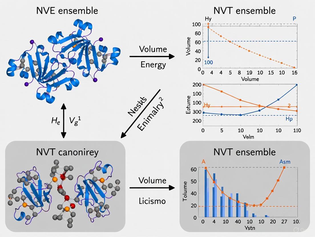
The following diagram illustrates the typical workflow and logical relationship between the NVE and NVT ensembles in a molecular dynamics simulation protocol, highlighting their distinct energy and temperature behaviors.

The Scientist's Toolkit: Essential Reagents and Methods

Table 3: Research Reagent Solutions for MD Ensemble Simulations

Item / Method	Function / Purpose
Velocity Verlet Algorithm [13]	A time-reversible integrator for numerically solving Hamilton's/EOMs; foundational for NVE and forms the basis for extended system NVT.
Nose-Hoover Chain Thermostat [13] [14]	An extended system method that adds fictitious thermodynamic variables to the Hamiltonian to correctly maintain constant temperature (NVT).
Liouvillian Formalism [13]	The theoretical framework for decomposing time evolution into position and momentum operators, enabling the derivation of stable integration algorithms.
Berendsen Thermostat [14]	A weak-coupling method that scales velocities to rapidly relax a system to a target temperature; often used for initial equilibration.
Thermostat Mass (Q) [14]	A parameter (e.g., ( Q = N{free} k T \taut^2 )) controlling the oscillation period of the thermostat; determines coupling strength and simulation stability.

The theoretical underpinnings of the NVE and NVT ensembles reveal a fundamental trade-off between physical isolation and experimental mimicry. The NVE ensemble, with its elegant Hamiltonian mechanics, is ideal for studying fundamental energy-conserving dynamics and probing a specific potential energy surface [10]. However, its inherent temperature fluctuations make it unsuitable for simulating most laboratory conditions. In contrast, the NVT ensemble's modified, non-Hamiltonian equations of motion, while more complex, are essential for modeling isothermal processes. The action of the thermostat is crucial, as it actively manages energy flow to maintain a constant temperature, de-correlating velocities and allowing the system to explore different regions of the PES that would be inaccessible in NVE [10]. This makes NVT indispensable for conformational searching and for computing properties at a specified temperature.

The choice between these ensembles is not merely academic but has direct implications for simulation outcomes. For instance, using NVE to equilibrate a system like a protein can lead to unstable temperature spikes that may cause unfolding, a problem mitigated by an NVT protocol [11]. Furthermore, while NVE can be used for production runs to analyze constant-energy surfaces, the NVT ensemble is often the default for data collection when periodic boundary conditions are used without significant pressure coupling, as it minimizes trajectory perturbation while maintaining a realistic thermodynamic state [1]. Ultimately, a comprehensive MD study often leverages both ensembles sequentially—using NVT for equilibration to a target temperature and then switching to NVE for production—highlighting that their distinct theoretical foundations are complementary tools in the computational scientist's arsenal.

In molecular dynamics (MD) simulations, statistical ensembles provide the foundational framework that defines the thermodynamic conditions of a system. These artificial constructs determine which quantities are held constant and which are allowed to fluctuate, directly influencing the simulation's behavior and the properties one can calculate [11] [1]. The choice between different ensembles is not merely a technical detail but a fundamental decision that aligns the computational experiment with either specific theoretical questions or realistic experimental conditions [7]. Among the most fundamental distinctions in MD is that between the microcanonical (NVE) and canonical (NVT) ensembles, which differ primarily in their treatment of energy and temperature.

The NVE ensemble conserves the total energy of an isolated system, making it the most straightforward implementation of Newton's equations of motion. In contrast, the NVT ensemble maintains a constant temperature by coupling the system to a thermal reservoir, effectively allowing energy to fluctuate [11] [10]. This core difference—energy conservation versus temperature maintenance—profoundly impacts the system's dynamics, the accessible thermodynamic properties, and the appropriate applications for each method. Within the broader context of ensemble difference research, understanding these distinctions is crucial for researchers, particularly in drug development where accurate simulation conditions can predict binding affinities, protein stability, and molecular interactions under physiological conditions [15] [16].

This technical guide provides an in-depth examination of the NVE and NVT ensembles, focusing on their theoretical foundations, practical implementations, and implications for computational research. We present structured comparisons, detailed experimental protocols, and visualization tools to equip scientists with the knowledge needed to select and implement the appropriate ensemble for their specific research objectives.

Theoretical Foundations: NVE and NVT Ensembles

The Microcanonical (NVE) Ensemble

The NVE ensemble describes completely isolated systems that cannot exchange energy or matter with their surroundings. In this ensemble, the Number of particles (N), Volume (V), and total Energy (E) remain constant throughout the simulation [11] [1]. Mathematically, systems in the NVE ensemble follow Hamilton's equations of motion, which conserve the Hamiltonian H(P,r) such that dH/dt = 0 [10]. This conservation law restricts the system to explore only those microstates associated with the total energy E, creating a constant potential energy surface throughout the simulation [10].

In practical terms, the NVE ensemble represents the most fundamental MD approach because it directly implements Newton's second law without additional constraints. However, this simplicity comes with significant behavioral consequences: as the system explores regions of different potential energy (PE) on the potential energy surface, the kinetic energy (KE) must change compensatorily to maintain constant total energy (E = KE + PE) [10]. These changes in kinetic energy directly translate to fluctuations in instantaneous temperature, since temperature in MD is calculated from atomic velocities [1]. Consequently, while total energy remains perfectly conserved (barring numerical errors), temperature becomes a fluctuating property that cannot be controlled, making NVE unsuitable for simulating isothermal conditions [10].

The Canonical (NVT) Ensemble

The NVT ensemble maintains constant Number of particles (N), Volume (V), and Temperature (T), representing a system that can exchange energy with a thermal reservoir at a fixed temperature [11] [1]. This ensemble differs fundamentally from NVE in that it follows non-Hamiltonian equations of motion where dH/dt ≠ 0, allowing the total energy to fluctuate while the temperature remains constant [10]. This approach mimics common experimental conditions where temperature is carefully controlled while energy exchange with the environment occurs naturally.

The constant temperature in NVT simulations is achieved through algorithmic thermostats that adjust atomic velocities to maintain the desired temperature. When a "rogue atom" acquires excessive kinetic energy, increasing local temperature, the thermostat removes this excess energy, effectively "pacifying" the atom to maintain the system at the target temperature [10]. Conversely, if the system's temperature drops below the target, the thermostat adds energy. This mechanism decouples the kinetic energy from potential energy changes, allowing the system to move through valleys and peaks on the potential energy surface without requiring compensatory temperature fluctuations [10]. This capability enables the system to potentially access different potential energy surfaces, particularly at elevated temperatures where increased kinetic energy can help overcome energy barriers [10].

Table 1: Fundamental Characteristics of NVE and NVT Ensembles

Feature	NVE Ensemble	NVT Ensemble
Conserved Quantities	Number of particles (N), Volume (V), Energy (E)	Number of particles (N), Volume (V), Temperature (T)
Energy Behavior	Constant total energy	Fluctuating energy
Temperature Behavior	Fluctuating temperature	Constant temperature
Equations of Motion	Hamiltonian (dH/dt = 0)	Non-Hamiltonian (dH/dt ≠ 0)
System Type	Isolated system	System connected to heat bath
Potential Energy Surface	Constant	Can transition between surfaces

Comparative Analysis: Thermodynamic and Dynamic Properties

Thermodynamic Properties and Sampling

While the NVE and NVT ensembles represent different thermodynamic conditions, they yield consistent results for many structural and energetic properties under appropriate conditions. Research comparing NVE and NVT simulations of amorphous polyether systems like tetraglyme has demonstrated that energy, temperature, and most structural features remain very similar between the two approaches [9]. This consistency arises because both ensembles sample from essentially the same configurational space when properly equilibrated, particularly for large systems where ensemble equivalence is expected in the thermodynamic limit [7].

However, important distinctions emerge in certain thermodynamic derivatives and fluctuation properties. The NVT ensemble typically provides more efficient sampling for systems with complex energy landscapes, as the temperature control mechanism helps prevent trapping in local minima. In NVE simulations, if a system becomes trapped in an energy valley, it lacks a mechanism to acquire the necessary kinetic energy to escape, potentially leading to inadequate sampling of phase space [10]. This sampling limitation can violate ergodicity principles where time averages should equal ensemble averages, ultimately affecting the accuracy of computed thermodynamic properties [10].

Dynamic Properties and Structural Differences

Despite similarities in structural properties, significant differences emerge in dynamic behaviors between NVE and NVT ensembles. Studies on tetraglyme have revealed "major differences in dynamic properties, i.e., in the mean square displacement and in the OO distances" [9]. These discrepancies arise fundamentally from how each ensemble handles energy transfer. In the NVT ensemble, the thermostat maintains constant temperature by continuously adding or removing energy from the system, which directly affects atomic velocities and consequently alters diffusion rates and other time-dependent properties [9] [10].

The constant velocity rescaling in NVT simulations effectively decorrelates atomic velocities, which while beneficial for temperature control, artificially perturbs the natural dynamics of the system [10]. This perturbation makes NVT less suitable for studying authentic dynamical processes or calculating properties derived from velocity correlation functions, such as infrared spectra [7]. For these applications, many researchers equilibrate the system in NVT and then switch to NVE for production dynamics to preserve genuine dynamic behavior while maintaining the desired temperature state [7].

Table 2: Comparison of Properties and Applications in NVE and NVT Ensembles

Property/Application	NVE Ensemble	NVT Ensemble
Structural Properties	Similar to NVT [9]	Similar to NVE [9]
Dynamic Properties	Natural dynamics	Perturbed dynamics [9] [10]
Energy Barriers	Cannot overcome barriers higher than initial energy [7]	Can overcome barriers via thermal energy [7]
Sampling Efficiency	Can get trapped in local minima [10]	Better for crossing barriers [10]
Recommended Applications	Gas-phase reactions, authentic dynamics, spectroscopy [7]	Biological systems, fixed-temperature studies [15] [7]
Free Energy Connection	Internal energy [7]	Helmholtz free energy [7]

Implementation and Methodological Considerations

Thermostat Implementation in NVT Simulations

Implementing the NVT ensemble requires selecting and configuring an appropriate thermostat algorithm to maintain constant temperature. Several thermostat types are available, each with distinct characteristics and applications:

• Berendsen Thermostat: A weak-coupling method that scales velocities periodically to adjust temperature toward the target value. It provides good convergence but uniformly changes velocity distributions across the entire system, which can produce unnatural dynamical behavior [17].
• Nosé-Hoover Thermostat: An extended system approach that incorporates the heat bath as an integral part of the system with additional degrees of freedom. This method原则上 reproduces the correct NVT ensemble and is widely applicable, though it may exhibit ergodicity issues in simple systems like harmonic oscillators [10] [17].
• Langevin Thermostat: A stochastic method that applies random forces to individual atoms based on Maxwell-Boltzmann distributions. It provides proper sampling for mixed-phase systems but is unsuitable for precise trajectory analysis due to its inherent randomness [17].
• Andersen Thermostat: Another stochastic approach that periodically reassigns velocities to random atoms from Maxwell-Boltzmann distributions. Effective for temperature control but similarly alters natural dynamics [10].

The choice among these thermostats depends on the specific research goals. For studies prioritizing correct dynamical behavior, minimal-interference thermostats like Nosé-Hoover are preferable, while for rapid equilibration, stochastic methods may be more effective.

Practical Simulation Workflows

A standard MD protocol typically employs both NVT and NVE ensembles at different stages to leverage their respective advantages [11]. The following diagram illustrates a typical workflow:

This workflow begins with energy minimization of the initial structure, followed by NVT equilibration to bring the system to the target temperature [11]. For condensed-phase systems, an additional NPT equilibration step often follows to achieve the correct density. Finally, production simulation occurs in either NVE or NVT ensemble depending on the target properties: NVE for authentic dynamic behavior or NVT for structural analysis at constant temperature.

Table 3: Essential Software and Force Fields for Ensemble Simulations

Tool Category	Specific Examples	Function in Ensemble Simulations
MD Software	GROMACS, LAMMPS, VASP, AMBER, BIOVIA Materials Studio	Provide integration algorithms, thermostat implementations, and analysis tools for different ensembles [9] [1] [18]
Force Fields	PCFF, CHARMM, AMBER, OPLS	Define potential energy functions governing atomic interactions; accuracy critical for both NVE and NVT [9] [15]
Thermostat Algorithms	Nosé-Hoover, Berendsen, Langevin, Andersen	Maintain constant temperature in NVT simulations through various velocity control mechanisms [10] [17]
Analysis Tools	VMD, MDAnalysis, in-built trajectory analyzers	Calculate thermodynamic and dynamic properties from simulation trajectories

Advanced Applications and Research Implications

Case Study: Pharmaceutical Research and Drug Development

The selection between NVE and NVT ensembles has practical significance in pharmaceutical research, particularly in structure-based drug design. In a recent study investigating neuromuscular blocking agents, researchers employed molecular dynamics simulations to examine binding stability between hit compounds and nicotinic acetylcholine receptors [16]. The choice of ensemble directly influenced the assessment of ligand-receptor complex stability and binding free energies calculated through MM/GBSA methods.

For such applications, NVT simulations are typically preferred because they maintain physiological temperature conditions (310 K for human body simulations), enabling more realistic modeling of biomolecular behavior [15] [16]. The constant temperature condition helps simulate the true thermodynamic environment in which drug-receptor interactions occur, providing more accurate predictions of binding affinities and residence times crucial for drug development.

Specialized Research Applications

Different research domains benefit from specific ensemble choices based on their particular requirements:

• Materials Science: NVT simulations are valuable for studying ion diffusion in solids, adsorption processes on slab surfaces, and reactions on clusters where volume changes are negligible [17]. The constant volume condition simplifies analysis of diffusion pathways and surface interactions.
• Spectroscopy Studies: NVE simulations are essential for calculating spectroscopic properties from velocity correlation functions, as thermostat interference in NVT would alter the natural dynamics underlying these properties [7].
• Phase Transitions: NPT ensembles (constant pressure and temperature) are typically preferred for studying phase transitions, though NVT can reveal how fixed volume constraints affect transition pathways [10].

The following diagram illustrates the decision process for selecting between NVE and NVT ensembles based on research objectives:

The distinction between NVE and NVT ensembles represents a fundamental aspect of molecular simulation methodology with far-reaching implications for computational research. The core difference—energy conservation in NVE versus temperature maintenance in NVT—manifests in significantly different dynamic behaviors while preserving similarities in many structural properties. This understanding is crucial for researchers across disciplines, particularly drug development professionals whose work relies on accurate molecular simulations.

The choice between ensembles should be guided by the specific research objectives, with NVE preferred for studying authentic dynamics and gas-phase systems, and NVT more appropriate for simulating biological conditions at constant temperature. As molecular simulation methodologies continue advancing, with developments in machine learning, quantum mechanics integration, and enhanced sampling techniques, both ensembles will remain essential tools in the computational scientist's arsenal. By understanding their fundamental differences and appropriate applications, researchers can make informed decisions that enhance the reliability and relevance of their computational findings to experimental observations.

This technical guide explores the fundamental role of statistical ensembles in defining a system's accessible microstates and behavior within phase space. Framed within a broader thesis contrasting the Microcanonical (NVE) and Canonical (NVT) ensembles, this work delineates their theoretical foundations, practical implementations in Molecular Dynamics (MD), and implications for system properties. We provide a comprehensive comparison of the NVE and NVT ensembles, detailing their governing principles, representative algorithms, and consequences for energy distribution and sampling. The analysis is supported by quantitative data tables, detailed experimental protocols, and visualizations of the underlying workflows, offering researchers a rigorous framework for selecting an appropriate ensemble for computational experiments, particularly in fields like drug development.

In statistical mechanics, a thermodynamic ensemble is a conceptual collection of all possible microstates of a system that satisfy a set of macroscopic constraints, such as constant energy or temperature [19]. These ensembles provide the foundational link between the microscopic laws of mechanics and macroscopic thermodynamic observables. The phase space for a classical system is a multidimensional space in which each point represents a complete state of the system, defined by all the positions (q) and momenta (p) of its N constituent particles. A microstate corresponds to a single point in this 6N-dimensional space, whereas a macrostate is described by a probability distribution over these points—the ensemble itself [19].

The system's evolution traces a trajectory through this phase space, and the ensemble defines a measure—the probability density—for regions of this space. The choice of ensemble, therefore, directly determines which microstates are accessible and with what probability, fundamentally shaping the system's observed behavior and properties [10]. This guide focuses on the two ensembles most critical for the initial analysis of isolated and closed systems: the Microcanonical (NVE) and Canonical (NVT) ensembles.

Theoretical Foundations: NVE vs. NVT

The Microcanonical (NVE) Ensemble

The NVE ensemble describes an isolated system that cannot exchange energy or particles with its surroundings. It is defined by a fixed number of particles (N), a fixed volume (V), and a fixed total energy (E) [19]. The fundamental postulate of statistical mechanics states that for such a system, all accessible microstates are equally probable. This is the only ensemble that directly mirrors the dynamics governed by Hamilton's equations of motion:

where H is the Hamiltonian of the system, and p and q are the momentum and position vectors, respectively [4]. For a common system, the Hamiltonian takes the form ( H(\boldsymbol{p},\boldsymbol{q}) = \sum{i=1}^{F} \frac{p{i}^{2}}{2m_{i}} + V(\boldsymbol{q}) ), representing the sum of kinetic and potential energies [4].

The primary thermodynamic potential for the NVE ensemble is entropy (S). Several definitions exist, with the Boltzmann entropy, ( SB = k{\text{B}} \log W ), being prominent. Here, ( k_{\text{B}} ) is Boltzmann's constant and W is the number of microstates within a small energy range around E [19]. In NVE, temperature is not a control parameter but a derived quantity, calculated from the derivative of entropy with respect to energy.

The Canonical (NVT) Ensemble

The NVT ensemble describes a closed system that can exchange energy, but not particles, with a much larger heat bath at a constant temperature (T) [10]. The system has a fixed number of particles (N), a fixed volume (V), and a fixed temperature (T). Because energy can fluctuate, the total energy (E) of the system is not constant.

The probability of the system being in a microstate with energy ( Ei ) is given by the Boltzmann distribution: [ Pi = \frac{e^{-Ei / kB T}}{\sumi e^{-Ei / k_B T}} ] This distribution implies that microstates with lower energy have a higher probability of being occupied [20]. The system's energy is allowed to fluctuate as it moves between these microstates. This ensemble does not, strictly speaking, follow Hamiltonian equations of motion unless extended to include the thermostat as part of the system. The connection to a heat bath makes the NVT ensemble the natural choice for simulating most experimental conditions, where temperature is a controlled variable [11].

Comparative Analysis: A Theoretical Viewpoint

The core of the thesis differentiating NVE and NVT lies in their treatment of energy and temperature. The NVE ensemble is fundamental, with its constant energy directly arising from the laws of classical mechanics for an isolated system. Its strength is its exact conservation of energy and symplectic structure, which leads to excellent long-time stability and accurate dynamics for short simulations [4]. However, it does not represent the constant temperature conditions of most real-world experiments.

Conversely, the NVT ensemble sacrifices strict energy conservation to maintain a constant temperature, which is a more common experimental control parameter. This makes it more practical for most applications, but the introduction of a thermostat can perturb the true dynamical trajectories of the particles [20]. The NVT ensemble can be seen as a system connected to an infinite external reservoir that supplies or removes energy to maintain a fixed T, leading to energy fluctuations that are negligible for large systems but can be significant for small ones.

Table 1: Theoretical Comparison of NVE and NVT Ensembles

Feature	Microcanonical (NVE) Ensemble	Canonical (NVT) Ensemble
Defined Macroscopic Variables	Constant N, V, E	Constant N, V, T
System Type	Isolated	Closed, in contact with a heat bath
Energy	Constant	Fluctuates around an average value
Temperature	Derived, fluctuates	Constant, imposed by the bath
Fundamental Potential	Entropy (S)	Helmholtz Free Energy (F)
Probability of a Microstate	Uniform for all accessible states	Boltzmann distribution
Governed by	Hamilton's equations of motion	Non-Hamiltonian equations (with thermostat)

Practical Implementation in Molecular Dynamics

NVE Molecular Dynamics

In MD, an NVE simulation is performed by integrating Newton's equations of motion without any temperature or pressure control algorithms [1]. Common integration algorithms like Verlet or Leapfrog are used. Because of numerical errors, the total energy might exhibit a slight drift, but in a well-converged simulation, this drift is minimal. The temperature in an NVE simulation is not controlled but can be calculated from the average kinetic energy of the particles: [ \langle T \rangle = \frac{2 \langle E{kin} \rangle}{kB N{dof}} ] where ( N{dof} ) is the number of degrees of freedom. This calculated temperature will fluctuate over time [10].

NVE MD is highly valued for producing accurate, unperturbed dynamical trajectories. It is often recommended for the production phase of a simulation if the goal is to study genuine dynamics, such as for calculating transport properties or for use with the fluctuation-dissipation theorem [20]. However, it is not ideal for equilibration, as it provides no mechanism to drive the system to a desired temperature [1].

NVT Molecular Dynamics

Implementing the NVT ensemble requires a thermostat to maintain a constant temperature by adjusting the system's kinetic energy. This is equivalent to simulating the energy exchange with a heat bath [10]. Several thermostat algorithms exist, each with different strengths and weaknesses:

• Berendsen Thermostat: A weak-coupling method that scales velocities periodically to push the temperature towards the desired value. It is efficient for equilibration but does not generate a correct canonical distribution [10].
• Nosé-Hoover Thermostat: An extended-system method that introduces an additional degree of freedom representing the heat bath. It generates a correct canonical ensemble and is widely used for production simulations [21].
• Stochastic Thermostats (e.g., Andersen): This method randomly assigns new velocities to particles from a Maxwell-Boltzmann distribution corresponding to the target temperature. It produces a correct canonical ensemble but can disrupt dynamics more significantly than deterministic methods [10].

In an NVT simulation, the potential energy can change as the system moves on the Potential Energy Surface (PES), but the kinetic energy does not have to compensate to keep the total energy constant. Instead, the thermostat adds or removes energy to maintain a constant temperature, allowing the total energy to fluctuate [10].

Table 2: Practical Comparison of NVE and NVT in Molecular Dynamics

Aspect	NVE MD	NVT MD
Integration Method	Newton's / Hamilton's equations	Non-Hamiltonian equations with thermostat
Temperature Control	None	Achieved via a thermostat algorithm
Energy Conservation	Excellent (barring numerical drift)	Not conserved; energy fluctuates
Primary Use Case	Production runs for accurate dynamics; studies of energy-conserving systems	Equilibration; simulating realistic experimental conditions
Effect on Dynamics	Produces genuine dynamical trajectories	Thermostat can perturb true dynamics
Sampling	Can be inefficient if stuck in a region of phase space	Easier barrier crossing due to energy exchange

Why NVT is Prevalent in Molecular Dynamics Literature

Despite the dynamical artifacts introduced by thermostats, the NVT ensemble is extremely common in MD, particularly for production runs in biomolecular simulations like drug development [20]. There are several practical reasons for this:

• Experimental Correspondence: Most real-world experiments, especially in biochemistry, are performed at constant temperature (e.g., physiological temperature), not constant energy. NVT simulations directly mimic these conditions [11].
• Numerical Stability and Equilibration: Maintaining a constant energy numerically is challenging due to the accumulation of integration errors. Thermostats help correct for this drift, providing a more stable simulation over long timescales [20].
• Enhanced Sampling: A constant temperature allows the system to more easily cross energy barriers. In NVE, if the system is initialized with a certain energy, it may be trapped in a specific region of phase space. The energy exchange in NVT facilitates better ergodic sampling, ensuring the system explores all relevant microstates [10].

A standard MD protocol often involves using the NPT ensemble (constant pressure and temperature) for equilibration to find the correct system density, followed by a switch to NVT for production runs to keep the simulation box size fixed, which simplifies the calculation of many properties [11] [20].

The Scientist's Toolkit: Essential Reagents and Algorithms

Table 3: Key Computational "Reagents" for Ensemble Simulations

Item	Type	Primary Function	Considerations
Verlet / Leapfrog Integrator	Algorithm	Integrates Newton's equations of motion for NVE dynamics.	Time-reversible and symplectic; excellent for energy conservation.
Nosé-Hoover Thermostat	Algorithm	Maintains constant temperature in NVT simulations.	Generates a correct canonical ensemble; can exhibit non-ergodicity in small systems.
Berendsen Thermostat	Algorithm	Weakly couples system to a heat bath for temperature control.	Efficient for equilibration; does not produce a rigorous canonical ensemble.
Andersen Thermostat	Algorithm	Maintains temperature by stochastic collision events.	Produces a correct canonical ensemble; can disrupt dynamic correlations.
Force Field (e.g., CHARMM, AMBER)	Parameter Set	Defines the potential energy function (PES) for the system.	Accuracy is paramount; choice depends on the system (proteins, lipids, materials).
Periodic Boundary Conditions	Simulation Setup	Mimics a macroscopic system by replicating the simulation box.	Eliminates surface effects; requires careful handling of long-range interactions.

Experimental Protocols and Workflows

Protocol for a Comparative NVE vs. NVT Study

This protocol outlines the steps to compare the thermodynamic and dynamic properties of a system simulated in both the NVE and NVT ensembles, as referenced in studies of amorphous polymers [9].

• System Preparation: Construct an initial configuration of the system (e.g., 16 tetraglyme molecules in an amorphous cell). Use a validated force field (e.g., PCFF for polymers).
• Energy Minimization: Perform a conjugate gradient minimization to remove high-energy clashes and strains in the initial structure.
• Equilibration in NVT:
  • Heat the system to the target temperature (e.g., 600 K).
  • Cool the system down to the desired simulation temperature (e.g., 300 K) over a sufficient timeframe.
  • Apply a thermostat (e.g., Nosé-Hoover) and run for a defined period to allow the system to equilibrate at the target temperature. Monitor potential energy and temperature for stability.
• Production Run - Branch A (NVT):
  • Using the equilibrated coordinates and velocities from Step 3, continue the simulation in the NVT ensemble for the desired production length (e.g., nanoseconds).
  • Trajectory data (positions, velocities, energies) are written to file at regular intervals for analysis.
• Production Run - Branch B (NVE):
  • Using the identical equilibrated coordinates and velocities from Step 3, start a new simulation in the NVE ensemble.
  • Run for the same duration as the NVT production run, saving trajectory data.
• Analysis:
  • Thermodynamic Properties: Calculate and compare the average and fluctuation of potential energy, kinetic energy, and total energy for both ensembles.
  • Structural Properties: Compute radial distribution functions (e.g., O-O RDF) to assess if the structural features are similar [9].
  • Dynamic Properties: Calculate the mean squared displacement (MSD) to compare diffusion coefficients. Note that significant differences are often observed here, with NVT potentially showing altered dynamics due to the thermostat [9].

The workflow for this comparative protocol is visualized below.

A Typical MD Protocol for Drug Development

In drug development, simulating a protein-ligand complex under physiological conditions is paramount. The following workflow is standard practice [11]:

• NVT Equilibration: The minimized system is heated to the target temperature (e.g., 310 K) using a thermostat. This step brings the system to the correct temperature before enabling pressure coupling.
• NPT Equilibration: The system is then equilibrated in the NPT ensemble to achieve the correct density (e.g., 1 bar). A barostat is used to adjust the volume. This ensures the system is at the correct temperature and pressure.
• NVT Production: For the production run, the simulation is often switched back to the NVT ensemble, using the box dimensions stabilized in the NPT phase. This fixes the volume, simplifying subsequent analysis of properties like binding affinities and root-mean-square deviation (RMSD) [20]. The trajectory from this stage is used for all scientific analysis.

The logical flow of this standard protocol is shown below.

The choice between the NVE and NVT ensembles is not merely a technicality but a fundamental decision that shapes the accessible region of phase space and the resulting system behavior. The NVE ensemble, with its constant energy and symplectic structure, is the gold standard for obtaining true dynamical trajectories and is rooted in the first principles of mechanics. In contrast, the NVT ensemble, through its connection to a heat bath and constant temperature, provides a more practical and relevant framework for simulating most experimental conditions, albeit at the cost of introducing non-Hamiltonian forces.

The broader thesis of NVE vs. NVT research highlights a core trade-off in computational physics: the fidelity to fundamental dynamical laws versus the practicality of simulating realistic thermodynamic environments. For researchers in drug development, where simulating biological systems at physiological conditions is essential, the NVT ensemble, often preceded by NPT equilibration, remains the indispensable workhorse. Understanding the core principles outlined in this guide enables scientists to make informed decisions about ensemble selection, correctly interpret simulation data, and ultimately derive more meaningful biological insights from their computational experiments.

Within molecular dynamics (MD) simulations, the choice of thermodynamic ensemble is a critical determinant of the physical relevance of the results. This technical guide examines the core differences between the microcanonical (NVE) and canonical (NVT) ensembles, framing them within the context of their correspondence to real-world experimental conditions. While the NVE ensemble describes isolated systems with constant energy, the NVT ensemble, through its use of thermostats, mimics the constant temperature conditions prevalent in laboratory experiments. This in-depth analysis provides researchers and drug development professionals with a structured comparison of these ensembles, detailed methodologies for their implementation, and guidance on selecting the appropriate ensemble for biomolecular simulation.

In molecular dynamics, a thermodynamic ensemble is an artificial construct that defines the collection of all possible system states under a specific set of macroscopic constraints [10]. These ensembles provide the foundational framework for connecting the microscopic details of atomistic simulations to macroscopic observables. The core differentiator between ensembles lies in which state variables—number of particles (N), volume (V), energy (E), temperature (T), or pressure (P)—are held constant, and which are allowed to fluctuate [1].

The NVE, or microcanonical ensemble, represents the most fundamental approach, directly arising from the numerical integration of Newton's equations of motion. In contrast, the NVT, or canonical ensemble, introduces a heat bath to maintain constant temperature, a condition that more closely aligns with most experimental setups in chemistry and biology [20]. The physical significance of selecting one ensemble over another lies in this direct connection to the environmental conditions a researcher seeks to emulate. For drug development professionals, this choice dictates whether simulation outcomes can be meaningfully compared to experimental data obtained from in vitro assays or physiological conditions, where temperature is rigorously controlled.

Theoretical Foundations of NVE and NVT Ensembles

The Microcanonical (NVE) Ensemble

The NVE ensemble is characterized by a constant number of atoms (N), a fixed volume (V), and a conserved total energy (E) [10] [18]. It represents a perfectly isolated system that cannot exchange energy or matter with its surroundings. In MD, this ensemble is generated by integrating Newton's equations of motion without any temperature or pressure control mechanisms [1].

The conservation of total energy, ( E = KE + PE ), is a defining feature. As atoms move on the Potential Energy Surface (PES), their potential energy (PE) fluctuates; to keep ( E ) constant, the kinetic energy (KE) must fluctuate in compensation [10]. Since temperature in MD is a statistical quantity derived from the average kinetic energy, these KE fluctuations cause the instantaneous temperature of the system to vary. The NVE ensemble is, therefore, not suitable for simulating isothermal conditions [10]. Its primary physical significance lies in modeling truly isolated systems or for probing fundamental dynamical properties where energy conservation is paramount [7].

The Canonical (NVT) Ensemble

The NVT ensemble maintains a constant number of atoms (N), a fixed volume (V), and a constant temperature (T) [10] [17]. It models a system in thermal contact with a heat bath, allowing energy exchange to maintain a fixed temperature [11]. This decouples the kinetic and potential energies; when a system moves to a region of higher potential energy on the PES, the thermostat provides the necessary energy, preventing a drop in kinetic energy and thus temperature [10].

This is achieved through various thermostat algorithms, which can be broadly categorized as follows [10] [17]:

• Strong Coupling (e.g., Velocity Rescaling): Directly scales atomic velocities relative to the desired temperature. It is effective but can introduce brutal, non-physical perturbations.
• Weak Coupling (e.g., Berendsen): Gently scales velocities periodically, offering better convergence but potentially producing unnatural velocity distributions.
• Stochastic Methods (e.g., Langevin): Applies random forces sampled from a statistical distribution (e.g., Maxwell-Boltzmann) to individual atoms. This is robust for mixed phases but unsuitable for precise trajectory analysis due to its statistical nature.
• Extended Systems (e.g., Nosé-Hoover): Treats the heat bath as an integral part of the system by introducing additional degrees of freedom. It is a rigorous method that, in principle, reproduces the correct NVT ensemble.

The NVT ensemble's physical significance is its direct mimicry of a vast number of real-world experimental conditions where temperature is a controlled variable, such as a reaction flask in a water bath or a biological assay in an incubator [20].

A Comparative Analysis: Physical Significance and Applicability

The core difference between NVE and NVT lies in their connection to the physical world. NVE simulates an idealization—a system perfectly insulated from its environment. In contrast, NVT simulates a common experimental reality—a system held at a constant temperature [20]. This fundamental distinction guides their application.

Table 1: Comparative Analysis of NVE and NVT Ensembles

Feature	NVE (Microcanonical) Ensemble	NVT (Canonical) Ensemble
Constant Parameters	Number of particles (N), Volume (V), Energy (E)	Number of particles (N), Volume (V), Temperature (T)
Fluctuating Quantities	Temperature (T), Pressure (P)	Energy (E), Pressure (P)
System Analogy	Isolated system	System in a heat bath
Physical Significance	Models idealized, energy-conserving systems; fundamental for studying dynamics	Mimics common lab conditions with controlled temperature
Primary MD Applications	Studying fundamental dynamics, probing PES, calculating properties via fluctuation-dissipation theorems [10]	Simulating most solution-phase chemistry, biomolecular processes, and systems where volume is fixed [17] [20]
Impact on Phase Space	System is confined to a single PES defined by the initial energy ( E ) [10]	System can access different PESs via energy exchange with the thermostat, enhancing conformational sampling [10]
Equations of Motion	Hamiltonian (conservative)	Non-Hamiltonian (dissipative)

For researchers, a key practical consideration is that the NVE ensemble is not recommended for system equilibration because, without energy flow, it cannot drive the system to a desired temperature starting from an arbitrary state [1]. Its strength lies in the production phase after equilibration, particularly for calculating dynamic properties where the artificial decorrelation of velocities by a thermostat would distort the results [7]. For instance, calculating an infrared spectrum from time correlation functions is best done in the NVE ensemble [7].

The NVT ensemble is the default choice for most production runs where constant temperature is the target, especially when the system volume is known and should remain fixed, such as in a rigid container or when studying a crystal lattice [17] [1]. It is also critical for computing properties related to the Helmholtz free energy [7].

Practical Implementation and Protocols

Essential Research Reagents and Computational Tools

The practical application of these ensembles relies on a suite of software and algorithmic "reagents."

Table 2: Key Research Reagent Solutions for Ensemble Simulations

Tool / Algorithm	Type	Primary Function	Considerations for Drug Development
Amber (pmemd) [22]	MD Software	GPU-accelerated engine for biomolecular simulation.	Industry standard for simulating proteins, nucleic acids, and protein-ligand complexes.
LAMMPS [10]	MD Software	A highly versatile and scalable MD simulator.	Suitable for a wide range of materials, including polymers and metals.
VASP [18]	MD/DFT Software	For ab initio MD simulations using quantum mechanics.	Used for simulating reactive processes and systems where electronic effects are critical.
Nosé-Hoover Thermostat [10] [17]	Algorithm (Extended System)	Rigorous temperature control by extending the system.	Reproduces correct NVT ensemble but may fail for small or specific systems.
Berendsen Thermostat [10] [17]	Algorithm (Weak Coupling)	Gently couples system to a heat bath for rapid convergence.	Good for equilibration but produces an artificial velocity distribution.
Langevin Thermostat [17]	Algorithm (Stochastic)	Controls temperature via random and friction forces on atoms.	Excellent for solvated systems but introduces stochastic noise into trajectories.
Andersen Thermostat [10] [18]	Algorithm (Stochastic)	Assigns random velocities from a Maxwell-Boltzmann distribution.	Effectively decorrelates velocities but can be overly disruptive to dynamics.

Detailed Experimental Protocol: System Equilibration and Production

A standard MD protocol for a biomolecular system, such as a protein-ligand complex, involves a multi-stage process to ensure proper equilibration before production data is collected [11]. The following protocol outlines a typical workflow.

Objective: To equilibrate a solvated protein-ligand system and run a production simulation under controlled, experimentally relevant conditions.

Software: Amber [22] or GROMACS.

System Preparation: A protein-ligand complex is solvated in a periodic box of water molecules (e.g., TIP3P) with counterions to neutralize the system's charge.

Step 1: Energy Minimization

• Purpose: Remove bad steric clashes and high-energy distortions from the initial structure.
• Method: Steepest descent or conjugate gradient algorithm (e.g., IBRION=1 or 2 in VASP [18]).
• Ensemble: Not applicable (energy minimization is not a dynamics step).

Step 2: NVT Equilibration

• Purpose: Gradually heat the system to the target temperature (e.g., 310 K for physiological conditions) and allow the solvent and ions to relax.
• Method: Run MD with a thermostat (e.g., Berendsen or Langevin) active. The volume and box shape are held fixed.
• Justification: "This ensemble should be chosen when one wants to ignore volume and temperature changes" during this initial thermalization phase [17]. It is the "appropriate choice when conformational searches of molecules are carried out in vacuum" or when pressure is not a significant factor [1].
• Duration: Typically 50-500 ps. Monitor until the system temperature stabilizes around the target value.

Step 3: NPT Equilibration

• Purpose: Adjust the system density and allow the simulation box size to relax to achieve the correct average pressure (e.g., 1 bar).
• Method: Run MD with both a thermostat and a barostat active. The box volume is allowed to fluctuate.
• Duration: Typically 100-1000 ps. Monitor until the system density and pressure stabilize.

Step 4: Production Run

• Purpose: Generate a long, stable trajectory for data collection and analysis of structural, dynamic, and thermodynamic properties.
• Method: The choice of ensemble (NVT or NVE) depends on the specific scientific question.
  • NVT Production Run: This is the most common choice for drug development applications. It maintains a constant temperature, mimicking laboratory conditions. The box size is fixed at the average volume obtained from the NPT equilibration. A thermostat like Nosé-Hoover or Langevin is used [17] [20].
  • NVE Production Run: Used if the goal is to study authentic dynamical behavior without the perturbation of a thermostat, for instance, when calculating transport properties or spectroscopic observables from correlation functions [7] [1]. The system is started from the equilibrated state from Step 3.

The selection of an ensemble is not merely a technicality but a fundamental choice that anchors a simulation in a specific physical reality. The NVE ensemble, conserving total energy, provides a window into the intrinsic dynamics of an isolated system, making it invaluable for studying fundamental physical properties where thermostat-induced artifacts must be avoided. The NVT ensemble, by maintaining a constant temperature, serves as a direct computational analogue for the vast majority of experimental conditions encountered in chemistry and biology.

For researchers and drug development professionals, this distinction is paramount. Simulating a protein-ligand binding event under NVT conditions directly relates to experimental measurements taken in a temperature-controlled assay. The structured workflow of equilibration under NVT and NPT, followed by a production run in either NVT or NVE, provides a robust methodological framework. The choice of production ensemble ultimately depends on whether the scientific question prioritizes correspondence to a real-world, constant-temperature experiment (NVT) or the need for pristine, unperturbed dynamical information (NVE). Understanding this physical significance is essential for designing meaningful simulations and interpreting their results in a biologically and pharmacologically relevant context.

Implementation and Use Cases: Setting Up NVE and NVT Simulations for Biomedical Systems

Molecular Dynamics (MD) simulation serves as a cornerstone computational technique across chemistry, materials science, and drug discovery, providing atomic-level insights into molecular behavior. The choice of thermodynamic ensemble—the set of statistical mechanical conditions under which a simulation is performed—profoundly influences the fidelity, stability, and biological relevance of the results. This technical guide delineates rigorous guidelines for selecting between the microcanonical (NVE) and canonical (NVT) ensembles, focusing on applications in gas-phase, liquid-phase, and biomolecular systems. Framed within the broader thesis of NVE versus NVT research, we demonstrate that the NVE ensemble, conserving energy and volume, is paramount for simulating isolated systems and studying inherent dynamics. In contrast, the NVT ensemble, maintaining constant temperature, is indispensable for modeling most experimental conditions, from biological processes to material properties at finite temperatures. The guide synthesizes current research, provides structured quantitative comparisons, details experimental protocols, and offers visualization tools to empower researchers in making informed decisions that bridge the gap between computational models and physical reality.

Molecular Dynamics (MD) simulates the time evolution of a system of atoms by numerically integrating Newton's equations of motion. The equations of classical mechanics form the foundation, where for a Hamiltonian H that is typically time-independent for a closed system, the evolution of positions (q) and momenta (p) is given by Hamilton's equations [4]: dp/dt = −∂H/∂q, dq/dt = ∂H/∂p

The thermodynamic ensemble defines the macroscopic state of the system—which thermodynamic quantities are held constant—and thereby controls the microscopic propagation of these atomic trajectories. The two primary ensembles considered here are:

• NVE Ensemble (Microcanonical): Isolated systems with constant Number of particles, Volume, and total Energy.
• NVT Ensemble (Canonical): Closed systems at thermal equilibrium with a heat bath, constant Number of particles, Volume, and Temperature.

The central thesis of ongoing research interrogates the practical and philosophical differences between these ensembles. While the NVE ensemble captures the natural, unperturbed dynamics of a system, the NVT ensemble, through its thermostat, mimics the constant temperature of most laboratory experiments and physiological conditions. The choice is not merely technical; it influences fundamental properties such as energy conservation, the character of fluctuations, and the representation of dynamic processes. This guide provides a structured framework for this critical choice, grounded in both statistical mechanics and practical application.

Theoretical Foundations: NVE and NVT Ensembles

The Microcanonical (NVE) Ensemble

The NVE ensemble represents a perfectly isolated system that cannot exchange energy or matter with its surroundings. In MD, this is implemented by using integrators that conserve the total energy, such as the Velocity Verlet algorithm [23]. A crucial parameter to monitor in NVE is the conservation of total energy; the curve should remain constant with only small, acceptable oscillations [23]. The NVE ensemble is considered the most straightforward from a simulation methodology standpoint, as it does not introduce external perturbations from thermostats or barostats [9].

The Canonical (NVT) Ensemble

The NVT ensemble models a system in contact with a thermal reservoir at a constant temperature. This is achieved by incorporating a thermostat, which adjusts the atomic velocities to maintain the target temperature. Common thermostats include:

• Nosé-Hoover Thermostat: A robust, universally used method that, in principle, reproduces the correct NVT ensemble [17]. It introduces an extended Lagrangian to mimic the heat bath.
• Berendsen Thermostat: A simple method with good convergence that scales velocities uniformly. However, it can produce unnatural phenomena as it does not generate a rigorous canonical distribution [17].
• Langevin Thermostat: Controls temperature by applying a random force and a friction term to individual atoms. This is suitable for mixed phases but is not reproducible due to its statistical nature and thus not ideal for precise trajectory analysis [17].

In NVT, the system's equilibrium temperature becomes independent of the initial velocities and couples to the reservoir temperature, allowing energy to be exchanged with the virtual heat bath [23].

Comparative Analysis: Statistical and Practical Considerations

The core difference between the ensembles lies in their treatment of energy and temperature. NVE preserves the total energy, allowing the instantaneous temperature, calculated from the kinetic energy, to fluctuate. In NVT, the temperature is fixed, and the total energy fluctuates. For large systems, relative fluctuations of thermodynamic parameters scale inversely with the square root of the system size. For instance, relative temperature fluctuations are given by [24]: ΔT² = kₙT²/(Ncᵥ)

Where kₙ is the Boltzmann constant, N is the number of particles, and cᵥ is the specific heat at constant volume per particle. For typical system sizes (N ~ 10⁴-10⁵), this results in relative fluctuations of less than 1% [24]. Research on amorphous polymer systems has shown that while NVE and NVT yield similar results for energy, temperature, and most structural features, major differences can be observed in dynamic properties, such as mean square displacement [9].

Table 1: Fundamental Characteristics of NVE and NVT Ensembles

Feature	NVE (Microcanonical) Ensemble	NVT (Canonical) Ensemble
Conserved Quantities	Number of particles (N), Volume (V), total Energy (E)	Number of particles (N), Volume (V), Temperature (T)
System Analogue	Isolated system	System in a heat bath
Energy Behavior	Total energy is constant	Total energy fluctuates
Temperature Behavior	Instantaneous temperature fluctuates	Temperature is constant (set by thermostat)
Primary Use Cases	Gas-phase simulations, studying inherent dynamics, energy conservation tests [11] [23]	Biomolecular simulations, liquids, modeling lab conditions [11] [17]
Key Algorithms/Integrators	Velocity Verlet	Nosé-Hoover, Berendsen, Langevin thermostats [17]

Guidelines for Ensemble Selection by System Type

Gas-Phase and Isolated Systems

For gas-phase simulations, such as studying molecular collisions, isolated clusters, or reactions in vacuum, the NVE ensemble is often the most appropriate choice. Its conservation of total energy directly mirrors the physical reality of an isolated molecular system. The NVE ensemble is also typically used for molecular reactions [25]. Furthermore, the NVE ensemble serves as an excellent testbed for evaluating the stability of a simulation setup and the suitability of the chosen time step, as any significant energy drift indicates numerical inaccuracies or instability.

Liquid-Phase and Condensed Matter Systems

Liquid-phase systems are inherently in thermal contact with their environment. Therefore, the NVT ensemble is the standard choice for simulating liquids under realistic conditions. It allows the system to maintain a constant temperature, which is crucial for obtaining correct thermodynamic and dynamic properties. For example, in simulations of water at various states (saturated liquid-vapor mixture, near-critical, and supercritical regions), the NVT ensemble is effectively employed to control the temperature during the equilibration process [26]. The choice of thermostat, however, is critical. The Langevin thermostat, which applies random forces to individual atoms, can be advantageous for complex liquid mixtures as it ensures proper thermalization of all components [17].

Biomolecular Systems (Proteins, DNA, Membranes)

Biomolecular processes occur at constant temperature (e.g., 310 K for the human body), making the NVT ensemble the unequivocal default for production simulations. It is used for simulating biological systems at physiological conditions [25]. A standard equilibration protocol for biomolecular systems often involves a multi-step process [11]:

• Energy Minimization: Relaxation of the initial structure to remove high-energy clashes.
• NVT Equilibration: Heating the system to the target temperature (e.g., 300 K or 310 K) while restraining heavy atom positions, followed by a period without restraints to allow the solvent and ions to equilibrate. This step brings the system to the desired temperature [11] [23].
• NPT Equilibration: Allowing the system density to adjust by applying constant pressure.
• Production Run: The final, long simulation in the NPT ensemble (constant physiological pressure and temperature) from which data for analysis is collected [11].

While NPT is the standard for production, the initial temperature coupling in this pipeline is achieved through NVT simulation. For certain studies focusing on the intrinsic dynamics of a protein in a fixed crystal lattice or a specific volume, NVT may be used throughout.

Table 2: Recommended Ensembles and Thermostats for Different System Types

System Type	Recommended Ensemble	Typical Thermostat Choices	Key Considerations
Gas-Phase / Isolated Clusters	NVE	Not Applicable	Best for energy conservation and studying unperturbed dynamics [25].
Liquids (Simple)	NVT	Nosé-Hoover, Berendsen	Nosé-Hoover for correct sampling; Berendsen for rapid equilibration [17].
Complex Liquids / Mixtures	NVT	Langevin	Effective for mixed phases as it controls temperature per atom [17].
Proteins / DNA (Equilibration)	NVT	Nosé-Hoover, Berendsen	Critical for heating and stabilizing temperature before pressure coupling [11].
Biomolecular Membranes	NPT (after NVT)	Nosé-Hoover	Requires constant pressure to allow area per lipid to equilibrate.

Practical Protocols and the Researcher's Toolkit

Workflow for System Equilibration

A robust MD protocol involves multiple stages to gradually bring the system to equilibrium. The following workflow, implementable in packages like GROMACS or QuantumATK, is considered a standard course of action [11] [23]:

Implementation Example: NVT Simulation with ASE

The following Python code snippet, using the Atomic Simulation Environment (ASE), demonstrates how to set up an NVT MD simulation for an aluminum crystal, employing the Berendsen thermostat [17]:

The Scientist's Toolkit: Essential Research Reagents

Table 3: Key Software and Algorithmic "Reagents" for Ensemble Control

Tool / Reagent	Type	Primary Function	Typical Application
Velocity Verlet	Integrator	Numerically integrates Newton's equations of motion with good energy conservation.	Core integrator for NVE simulations; basis for many thermostated integrators [23].
Nosé-Hoover Thermostat	Thermostat	Generates a correct canonical (NVT) ensemble using an extended Lagrangian.	Default choice for NVT production runs in biomolecular and materials simulations [17] [23].
Berendsen Thermostat	Thermostat	Weakly couples the system to a bath by scaling velocities. Provides rapid convergence.	Useful for initial equilibration and heating stages due to its strong damping [17] [11].
Langevin Thermostat	Thermostat	Controls temperature via random and frictional forces on individual atoms.	Ideal for systems with complex dynamics, like polymers, or when using stochastic dynamics [17].
LAMMPS	MD Engine	A highly versatile and performant open-source MD simulator.	Supports all common ensembles and thermostats; widely used in academia and industry.
GROMACS	MD Engine	A high-performance package optimized for biomolecular systems.	Implements the standard NVT/NPT equilibration protocol for proteins, lipids, etc. [11].

Advanced Topics and Future Directions

Machine Learning and Structure-Preserving Integrators

A significant frontier in MD is the use of machine learning (ML) to learn accurate and efficient interatomic potentials. A key challenge with ML-driven MD has been the failure of non-structure-preserving models to conserve energy and maintain physical fidelity over long timescales [4]. Recent research proposes learning data-driven, structure-preserving (symplectic and time-reversible) maps, which is equivalent to learning the mechanical action of the system. This approach eliminates pathological behavior like energy drift and loss of equipartition, demonstrating that incorporating the geometric structure of Hamiltonian mechanics is crucial for stable, long-time-step simulations, even within an ML framework [4].

Understanding and Leveraging Fluctuations

In finite-size systems simulated by MD, thermodynamic fluctuations are inevitable. Their magnitude is inversely proportional to the square root of the system size. For instance, relative pressure fluctuations in an ideal gas are given by (ΔP/P)² = γ/N, where γ is the adiabatic exponent [24]. Understanding this is critical when interpreting results, especially near phase transitions where anomalies like van der Waals loops on a P-V curve can be at the same level as the intrinsic noise. Researchers must ensure that observed phenomena are statistically significant relative to these inherent fluctuations [24].

Decision Framework for Ensemble Selection

The following diagram synthesizes the guidelines presented in this paper into a logical decision framework to aid researchers in selecting the appropriate ensemble:

The choice between the NVE and NVT ensembles is a fundamental decision that directly impacts the physical validity and interpretability of an MD simulation. This guide has established that the NVE ensemble, conserving total energy, is the tool of choice for simulating isolated systems and for probing the intrinsic, unthermostated dynamics of a molecular system. The NVT ensemble, enforcing constant temperature, is essential for simulating the vast majority of experimental and biological conditions, where temperature is a controlled variable. The broader thesis of NVE-versus-NVT research underscores that there is no universal "best" ensemble; the optimal choice is inherently dictated by the research question and the physical system being modeled. By adhering to the guidelines, protocols, and decision framework provided, researchers can navigate this critical choice with confidence, ensuring their computational models are both theoretically sound and directly relevant to the real-world phenomena they seek to understand.

Within the broader research on the differences between NVE and NVT ensembles, the process of system equilibration stands as a critical bridge between initial configuration and production simulation. The choice between the microcanonical (NVE) and canonical (NVT) ensembles profoundly impacts both the equilibration pathway and the quality of sampling achieved. While these ensembles are theoretically equivalent in the thermodynamic limit for large systems, practical molecular dynamics simulations with finite particles and timescales exhibit significant differences in their approach to equilibrium [7]. This technical guide examines strategies for rapid and robust sampling during equilibration, contextualized within the NVE versus NVT paradigm, to provide researchers with methodologies for achieving reliable ensemble averages that properly represent the thermodynamic state of interest.

The fundamental distinction between these ensembles lies in their conserved quantities: NVE simulations conserve total energy, making them suitable for isolated systems but challenging for temperature control, while NVT simulations maintain constant temperature through thermal coupling to an external bath, better mimicking common experimental conditions [27] [1]. As noted in foundational literature, "Constant-energy simulations are not recommended for equilibration because, without the energy flow facilitated by the temperature control methods, the desired temperature cannot be achieved" [1]. This makes NVT typically preferred for equilibration, though some practitioners use NVE for production runs after proper equilibration to avoid perturbations from thermostats [1].

Theoretical Foundation: Ensemble Equivalence and Practical Considerations

Thermodynamic Basis for Ensemble Selection

The theoretical justification for ensemble selection rests on the principle of ensemble equivalence in the thermodynamic limit, though practical simulations operate with finite systems where differences emerge. The NVE ensemble, conserving the system's total energy, follows directly from Newton's equations of motion without external controls [1]. In contrast, the NVT ensemble maintains constant temperature through coupling to a thermal reservoir, enabling better control over thermodynamic state conditions relevant to experimental setups [17] [27]. Research on polyether systems has demonstrated that while NVE and NVT yield similar results for energy, temperature, and most structural features, "major differences were observed in dynamic properties, i.e., in the mean square displacement" [9].

Practical Implications for Sampling

The practical implications of ensemble choice significantly impact sampling quality and efficiency. NVT simulations typically reach equilibrium faster because temperature control provides a mechanism for energy exchange that helps overcome barriers in the energy landscape [7] [1]. For instance, in a system where a barrier height approaches the total energy available in NVE simulation, the rate of crossing would be zero, whereas in NVT, thermal fluctuations provide the necessary energy for barrier crossing [7]. This makes NVT particularly valuable for systems with complex energy landscapes, such as polymers or biomolecules, where complete sampling is challenging [9].

Table: Key Differences Between NVE and NVT Ensembles for Equilibration

Characteristic	NVE Ensemble	NVT Ensemble
Conserved Quantities	Number of particles (N), Volume (V), Energy (E)	Number of particles (N), Volume (V), Temperature (T)
Temperature Control	Fluctuates naturally	Maintained constant via thermostat
Equilibration Speed	Slower, no mechanism for energy exchange with bath	Faster, thermal coupling facilitates approach to equilibrium
Suitability for Initial Equilibration	Not recommended [1]	Preferred method [1]
Effect on Dynamic Properties	Preserves natural dynamics	May alter dynamics depending on thermostat choice [9]
Implementation Complexity	Simple (direct integration)	Requires thermostat algorithm

Equilibration Methodologies and Protocols

Staged Equilibration Approach

A robust equilibration strategy typically employs a staged approach that may transition between ensembles at different phases. A common protocol involves:

• Energy Minimization: Initial steepest descent or conjugate gradient minimization to remove bad contacts and high-energy configurations [28].
• Solvent Equilibration: For solvated systems, initial equilibration of solvent molecules around solute with position restraints on solute atoms.
• NVT Equilibration: System heating to target temperature using appropriate thermostats [1].
• NPT Equilibration (if needed): Density adjustment through pressure coupling, particularly for biomolecular systems where correct density is essential [29].
• Production: Either NVE or NVT based on research objectives, with NVE sometimes preferred for unperturbed dynamics after equilibration [1].

This multi-stage approach recognizes that different thermodynamic variables reach equilibrium on different timescales, with structural variables typically equilibrating slower than kinetic temperature [9].

Advanced Techniques for Challenging Systems

For systems with complex energy landscapes or slow dynamics, such as amorphous polymers or biomacromolecules, specialized equilibration techniques may be necessary:

The CRASH Method: Research on polyether systems demonstrated that interrupting an NVE simulation and reassigning velocity distributions to particles enabled faster equilibration of amorphous systems [9]. This approach produced a sharp transition in average potential energy, rapidly advancing the system toward equilibrium.

Hybrid Temperature Control: Combining different thermostats at different stages can optimize equilibration. For instance, using aggressive thermostats like Berendsen for initial heating due to its good convergence properties, then switching to more physically rigorous thermostats like Nosé-Hoover for production phases [17].

Targeted Sampling: For specific properties or regions of interest, techniques like metadynamics or replica exchange can enhance sampling of conformational space, though these extend beyond standard equilibration protocols [28].

Implementation Protocols and Technical Considerations

Thermostat Selection and Configuration

The choice of thermostat significantly impacts equilibration quality and sampling fidelity. Different thermostats offer distinct trade-offs between sampling efficiency and perturbation of natural dynamics:

Table: Comparison of Common Thermostats for NVT Equilibration

Thermostat	Mechanism	Advantages	Limitations	Recommended Use
Berendsen [17]	Scales velocities uniformly	Fast convergence, simple implementation	Produces unphysical velocity distributions	Initial equilibration stages
Nosé-Hoover [17] [30]	Extended Lagrangian with dynamical variables	Reproduces correct NVT ensemble in most cases	May exhibit non-ergodicity in simple systems [17]	Production equilibration and sampling
Langevin [17]	Applies random and frictional forces	Good for mixed-phase systems, robust	Alters dynamics, stochastic (non-reproducible)	Complex systems, enhanced sampling
NHC (Nosé-Hoover Chains) [30]	Multiple coupled thermostats	Improved ergodicity over standard Nosé-Hoover	Increased complexity	Systems with stiff degrees of freedom

Practical Implementation Example

For a typical biomolecular system, the following NVT equilibration protocol could be implemented using modern simulation packages:

This protocol emphasizes the critical steps: proper velocity initialization, momentum correction, and appropriate thermostat coupling parameters. The thermostat coupling parameter (taut) should be chosen carefully – too strong coupling (small taut) may overly perturb dynamics, while too weak coupling (large taut) may poorly control temperature [17].

Visualization of Equilibration Workflows

NVT Equilibration Protocol

NVT Equilibration Workflow

Ensemble Transition Strategy

Ensemble Transition Strategy

Table: Essential Components for Molecular Dynamics Equilibration

Component	Function	Implementation Examples
Thermostats	Control system temperature during NVT simulations	Berendsen, Nosé-Hoover, Langevin, Nosé-Hoover Chains [17] [30]
Barostats	Control system pressure (for NPT simulations)	Berendsen, Parrinello-Rahman (not covered in detail here)
Force Fields	Define interatomic interactions and potential energy	PCFF for polymers [9], AMBER/CHARMM for biomolecules [28]
Integrators	Numerically solve equations of motion	Verlet, Leapfrog [1] [28]
Constraint Algorithms	Freeze specific degrees of freedom (e.g., bonds with hydrogen)	SHAKE, RATTLE, LINCS [28]
Analysis Tools	Monitor equilibration progress and convergence	Energy, temperature, pressure, RMSD tracking

Effective equilibration strategies are fundamental to obtaining meaningful results from molecular dynamics simulations, with the choice between NVE and NVT ensembles representing a critical decision point in protocol design. While NVT ensembles generally offer superior equilibration performance due to their ability to exchange energy with a thermal reservoir, understanding the strengths and limitations of both approaches enables researchers to design appropriate simulation strategies. The staged equilibration approach, combining careful system preparation, appropriate thermostat selection, and rigorous convergence monitoring, provides a pathway to robust sampling across diverse molecular systems. As molecular simulations continue to evolve with advanced machine learning approaches [30] [31] and increasingly complex applications, these foundational equilibration principles remain essential for generating thermodynamically valid ensemble averages that properly represent the system under investigation.

In molecular dynamics (MD), the choice of thermodynamic ensemble is foundational, defining the state variables that remain constant during a simulation and determining the physical relevance of the results. The microcanonical (NVE) ensemble, which conserves the number of particles (N), volume (V), and energy (E), represents an isolated system. It is generated by integrating Newton's equations of motion without external controls and is characterized by conserved total energy, though potential and kinetic energy can fluctuate against each other [1] [11]. While NVE is vital for studying genuine dynamical properties without the perturbation of a thermostat, its practical use is limited because most experiments are conducted at constant temperature, not constant energy [7] [11].

The canonical (NVT) ensemble, which maintains a constant number of particles (N), volume (V), and temperature (T), addresses this limitation. It mimics a system coupled to an external heat bath, allowing energy exchange to maintain the temperature [1] [11]. This ensemble is crucial for mimicking most experimental conditions and for performing conformational searches [1]. The connection between NVE and NVT is theoretically established in the thermodynamic limit for an infinite system size [7]. However, for the finite-sized systems typical in MD simulations, the choice of the algorithm, or thermostat, used to maintain constant temperature in NVT simulations is non-trivial and significantly influences the quality of the sampling, the accuracy of dynamical properties, and the correctness of the generated ensemble [7] [8].

This guide provides an in-depth technical comparison of four prevalent thermostats—Nose-Hoover, Berendsen, Langevin, and Bussi-Donadio-Parrinello—focusing on their implementation, their impact on sampling within the NVT ensemble, and their suitability for different research goals in drug development and materials science.

Thermostat Fundamentals and Classification

Thermostats allow energy to enter and leave the simulated system to maintain the target temperature by adjusting particle velocities [8]. The methods fall into four broad categories [8] [10]:

• Extended System Methods: These incorporate the heat bath as an integral part of the system by adding additional degrees of freedom to the equations of motion. The primary example is the Nose-Hoover thermostat [32] [8].
• Stochastic Methods: These methods employ random forces to mimic interactions with a heat bath. The Langevin and Andersen thermostats are prominent examples [32] [8].
• Weak Coupling Methods: This approach scales velocities by a factor that gently steers the system temperature toward the target value. The Berendsen thermostat is the archetypal weak coupling method [33] [8].
• Strong Coupling Methods: These methods, such as simple velocity rescaling, enforce the target temperature strictly at each step, but they are not recommended for production dynamics as they do not generate a correct canonical ensemble [8].

Table 1: Core Characteristics of the Four Thermostats

Thermostat	Algorithm Type	Key Controlling Parameter(s)	Ensemble Sampled	Momentum Conservation
Nose-Hoover	Extended System	Thermostat "mass" / timescale (τ) [32] [6]	Canonical (NVT) [8] [6]	Yes [8]
Berendsen	Weak Coupling	Temperature relaxation time (τₜ) [33] [8]	Not well-defined (over-damped) [33] [6]	Yes
Langevin	Stochastic	Friction / damping coefficient (γ) [32] [6]	Canonical (NVT) [8]	No [8]
Bussi-Donadio-Parrinello	Stochastic	Coupling period / time constant [8] [6]	Canonical (NVT) [8] [6]	Yes (in typical implementation)

The following diagram illustrates the logical workflow for selecting an appropriate thermostat based on the research objective, which is a critical decision in setting up an NVT simulation.

In-Depth Thermostat Analysis

Nose-Hoover Thermostat

The Nose-Hoover thermostat is an extended system method that integrates the heat bath into the dynamics by introducing an additional degree of freedom, often conceptualized as a fictional "heat bath mass" [32] [8]. This approach modifies the equations of motion to produce a time-reversible, deterministic dynamics that rigorously generates a canonical ensemble [8] [6].

A key strength of Nose-Hoover is that it conserves momentum and does not inherently disrupt correlated motions, leading to a more natural system dynamics compared to stochastic methods [8]. This makes it an excellent choice for calculating transport properties and studying kinetics [32]. However, a potential drawback is that a single Nose-Hoover thermostat can exhibit non-ergodic behavior for simple systems like the harmonic oscillator. This is commonly addressed by using a Nose-Hoover chain, where multiple thermostats are coupled in a chain, each with its own mass parameter, to ensure proper ergodicity [32] [6]. The coupling strength is controlled by a "thermostat timescale" parameter; a larger value means weaker coupling and less interference with the natural dynamics, which is crucial for accurate measurement of dynamical properties [6].

Berendsen Thermostat

The Berendsen thermostat employs a weak coupling algorithm. It scales the velocities of all particles at each time step by a factor λ that is proportional to the difference between the instantaneous and target temperatures [33] [8]. This method provides exponential relaxation of the temperature toward the desired value, with the rate controlled by the coupling parameter τₜ (the temperature relaxation time) [33].

The primary advantage of the Berendsen thermostat is its robustness and rapid equilibration. It efficiently drives the system to the target temperature and is very effective for the initial heating or cooling stages of a simulation [8]. However, its critical weakness is that it does not produce a correct canonical ensemble [33] [6]. By suppressing the natural temperature fluctuations, it generates an energy distribution with a lower variance than that of a true NVT ensemble [8]. Consequently, its use should be restricted to equilibration phases only, and it is not recommended for production simulations where accurate ensemble averages are required [6].

Langevin Thermostat

The Langevin thermostat is a stochastic method that mimics the viscous interaction of particles with a solvent. It modifies Newton's equations of motion by adding two forces: a frictional force (proportional to the velocity via a damping coefficient, γ) and a random force [32] [8] [6]. The balance between these two forces is calibrated to ensure correct sampling of the canonical ensemble [8].

A key feature of the Langevin thermostat is that it couples individually to each particle. This provides a very tight and robust temperature control, which can be advantageous for stabilizing unstable systems or for sampling ensembles [6]. However, this same property means it does not conserve momentum and significantly suppresses the natural, correlated dynamics of the system [8]. This suppression makes it a poor choice for calculating dynamical properties like diffusion coefficients or for studying processes where collective motions are important [32] [6]. It is primarily used for structure generation or in situations where a robust thermal coupling is paramount, and dynamical accuracy is secondary [6].

Bussi-Donadio-Parrinello Thermostat

The Bussi-Donadio-Parrinello thermostat, also known as the stochastic velocity rescaling thermostat, can be viewed as a stochastic variant of the Berendsen method that has been corrected to sample the canonical ensemble correctly [8] [6]. It operates by rescaling the velocities of all particles by a random factor, which is chosen to ensure the kinetic energy distribution matches that of the canonical ensemble [8].

This thermostat combines the robust temperature control of the Berendsen method with the theoretical correctness of the Nose-Hoover and Langevin thermostats [6]. A significant advantage is that, in its typical implementation, it conserves momentum, which helps preserve the natural dynamics of the system better than the Langevin thermostat [8]. It is considered a modern and generally reliable choice for NVT production simulations, particularly when the stability of the Nose-Hoover thermostat is a concern.

Table 2: Detailed Comparison for Application in Research and Development

Aspect	Nose-Hoover	Berendsen	Langevin	Bussi-Donadio-Parrinello
Recommended Use Case	Production runs studying dynamics & kinetics [32] [8]	Initial equilibration only [6]	Structure generation; systems requiring robust control [6]	General production runs; robust canonical sampling [8] [6]
Impact on Dynamics	Minimal when weakly coupled; preserves correlated motion [8]	Over-damped, unphysical dynamics [33]	Significant suppression; impairs correlated motion [32] [6]	Moderate impact, better than Langevin [8]
Parameter Guidance	Timescale (τ): Use larger values (e.g., ~100 fs) for dynamical properties [6]	Relaxation time (τₜ): ~0.1 ps is typical; small τₜ causes strong damping [33]	Friction (γ): Low values for less interference [6]	Coupling period: Similar to Berendsen's τₜ [8]
Pros	Correct ensemble; natural dynamics; momentum conservation [8]	Fast, robust convergence to target T [33] [8]	Very robust temperature control; correct ensemble [6]	Correct ensemble; robust control; momentum conservation [8] [6]
Cons	Can exhibit oscillations; requires chains for ergodicity [32] [6]	Incorrect ensemble; suppressed fluctuations [33] [8]	Destroys dynamics; does not conserve momentum [32] [8]	Less natural dynamics than Nose-Hoover [8]

Practical Implementation and Protocols

The Scientist's Toolkit: Essential Research Reagents

The following table lists key software and conceptual "reagents" essential for implementing thermostat protocols in MD research.

Table 3: Essential Research Reagents for MD Thermostat Implementation

Item Name	Function / Relevance
Molecular Dynamics Engine	Software (e.g., GROMACS, NAMD, LAMMPS, QuantumATK) that performs numerical integration of equations of motion and implements thermostat algorithms [8] [6].
Thermostat Coupling Parameter	An empirical parameter (e.g., τ, γ) that controls the strength of coupling to the heat bath and must be carefully selected to balance control with natural dynamics [33] [6].
Initial Configuration	The starting atomic coordinates and velocities for the simulation, often drawn from a Maxwell-Boltzmann distribution at the target temperature [6].
Equilibrated System	A system that has reached a stationary state at the desired temperature (and pressure) after initial relaxation; essential for valid production data collection [6].

Detailed Methodology for a Standard NVT Simulation Protocol

A typical MD procedure involves multiple stages using different ensembles and thermostats to properly prepare the system [11].

• System Preparation: Construct the initial atomic configuration (e.g., a protein in a water box) and minimize its potential energy to remove high-energy clashes.
• Initial Equilibration (NVT):
  • Objective: Gently heat the system from a low initial temperature (e.g., 0 K) to the target temperature (e.g., 300 K) and allow the particle velocities to relax.
  • Thermostat Choice: The Berendsen thermostat is often suitable here due to its robust and exponential relaxation properties [8] [6].
  • Parameterization: A temperature relaxation time (τₜ) on the order of 0.1 ps is a typical starting point [33]. The simulation should run for a duration long enough for the temperature to stabilize (e.g., tens to hundreds of picoseconds).
• Production Simulation (NVT):
  • Objective: Generate a trajectory for data collection and analysis of structural and dynamical properties.
  • Thermostat Choice:
    • For studying dynamics and kinetics (e.g., diffusion, conformational changes), the Nose-Hoover chain thermostat is the preferred choice due to its minimal interference with natural dynamics [32] [8]. Use a coupling timescale parameter of 100 fs or more to ensure weak coupling [6].
    • If robust and simple canonical sampling is the primary goal and exact dynamics are less critical, the Bussi-Donadio-Parrinello thermostat is an excellent and reliable alternative [8] [6].
  • Validation: Always monitor the temperature and energy fluctuations to ensure stability. For Nose-Hoover, check for oscillations and consider increasing the chain length if necessary [6].

The choice of thermostat in an NVT simulation is a critical decision that directly impacts the physical correctness and interpretability of the results, especially when framed against the benchmark of NVE dynamics. The Nose-Hoover thermostat, particularly with chains, stands out for production simulations where the accurate reproduction of dynamical properties is essential. The Berendsen thermostat remains a useful tool for rapid equilibration but must be avoided in production runs. The Langevin thermostat offers robust control for ensemble sampling at the cost of native dynamics, while the Bussi-Donadio-Parrinello thermostat provides a modern and robust stochastic alternative for correct canonical sampling. By aligning the thermostat's characteristics with the research objectives, as guided by the framework provided, scientists can ensure their simulations yield meaningful and reliable insights.

Molecular dynamics (MD) simulation has become an indispensable tool in modern drug discovery, providing atomic-level insights into the behavior of therapeutic targets and their interactions with small molecules. The fundamental choice of thermodynamic ensemble directly impacts the biological relevance and accuracy of these simulations. While the microcanonical (NVE) ensemble conserves total energy and serves as the foundation of MD, it presents significant limitations for modeling biological systems that naturally exist in isothermal environments. In contrast, the canonical (NVT) ensemble maintains constant temperature through coupling to a thermal bath, making it uniquely suited for simulating ligand-protein binding under physiologically relevant conditions [7] [11] [1].

Theoretical considerations suggest that in the thermodynamic limit of infinite system size, different ensembles should yield equivalent results. However, in practical MD simulations with finite system sizes, the choice between NVE and NVT ensembles significantly impacts both the sampling of conformational states and the calculated thermodynamic properties [7]. For drug discovery applications, where accurate quantification of binding affinities and mechanisms is paramount, the NVT ensemble provides crucial advantages by mimicking the constant temperature conditions of experimental biological systems and facilitating more efficient exploration of the energy landscape relevant to ligand binding [11] [34].

Theoretical Foundation: NVE vs. NVT Ensembles in Biological Simulations

Fundamental Ensemble Characteristics

The microcanonical (NVE) ensemble represents a completely isolated system with constant number of particles (N), constant volume (V), and constant energy (E). In MD simulations, this is achieved by directly integrating Newton's equations of motion without temperature or pressure control [1]. While mathematically elegant, this approach suffers from practical limitations in biological simulations. Energy conservation is compromised by numerical integration errors, leading to temperature drift throughout simulations [1]. More critically, the inability to exchange energy with a environment makes NVE simulations poorly suited for modeling biological systems that naturally maintain constant temperature [11].

The canonical (NVT) ensemble maintains constant temperature through coupling to a thermal reservoir, typically implemented via thermostating algorithms that scale atomic velocities to maintain the desired temperature [11]. This approach directly mirrors experimental conditions where biological systems are studied at constant temperature, making NVT simulations more appropriate for calculating experimentally relevant thermodynamic properties [7]. The NVT ensemble samples the Helmholtz free energy rather than the internal energy sampled by NVE, providing a more relevant thermodynamic potential for understanding binding processes at constant temperature [7].

Practical Implications for Ligand-Protein Binding Studies

The choice between NVE and NVT ensembles has direct consequences for simulating ligand-protein interactions:

• Barrier crossing: In NVE simulations with total energy just below the activation barrier for a conformational change, the transition rate is essentially zero. In NVT simulations at the same average energy, thermal fluctuations enable barrier crossing, leading to more realistic sampling of rare events [7].
• Temperature control: NVT simulations prevent unrealistic temperature spikes that can occur during energy minimization in NVE simulations, particularly important for maintaining protein structural integrity [11].
• Experimental correspondence: Most laboratory experiments, including those measuring protein-ligand binding, are conducted at constant temperature, making NVT simulations more directly comparable to experimental results [7] [34].

Table 1: Comparison of NVE and NVT Ensembles for Ligand-Protein Binding Simulations

Characteristic	NVE Ensemble	NVT Ensemble
Conserved Quantities	Number of particles (N), Volume (V), Energy (E)	Number of particles (N), Volume (V), Temperature (T)
Thermodynamic Potential	Internal Energy	Helmholtz Free Energy
Temperature Behavior	Fluctuates, prone to drift	Maintained constant via thermostating
Experimental Correspondence	Isolated systems	Most biological experiments
Barrier Crossing	Limited by initial energy	Enabled by thermal fluctuations
Implementation Complexity	Simple Newtonian dynamics	Requires thermostat algorithms

Implementing NVT Simulations for Ligand-Protein Systems

Thermostat Selection and Configuration

Proper implementation of NVT simulations requires careful selection and parameterization of thermostats. Common thermostat algorithms include:

• Nosé-Hoover thermostat: Provides rigorous sampling of the canonical ensemble through extended Lagrangian dynamics. Recommended parameters include a relaxation time of 0.5-2.0 ps for biomolecular systems [35] [1].
• Langevin thermostat: Utilizes random forces and friction to maintain temperature, particularly effective for systems with diverse timescales. Suitable for simulating complex biomolecular systems where efficient thermalization is required [35].

The choice of thermostat parameters significantly impacts both sampling efficiency and dynamical properties. Overly strong coupling (short relaxation times) can suppress natural temperature fluctuations, while weak coupling may insufficiently control temperature [35]. For protein-ligand binding studies, it is often advisable to apply thermostats only to degrees of freedom perpendicular to relevant reaction coordinates to minimize interference with the binding process.

Standard Simulation Protocol for Ligand-Protein Binding

A typical MD protocol for studying ligand-protein interactions employs multiple stages with different ensembles:

• Energy minimization: Removes steric clashes and prepares the system for dynamics, typically performed without ensemble constraints.
• NVT equilibration: Brings the system to the target temperature while maintaining fixed volume, allowing proper thermalization before pressure coupling [11].
• NPT equilibration: Adjusts density to the target pressure, completing system equilibration.
• Production simulation: Generates trajectory data for analysis, which may use NVT, NPT, or NVE ensembles depending on the specific scientific questions [11] [1].

This multi-stage approach ensures proper equilibration of both temperature and density before production simulations, critical for obtaining physically meaningful results [11].

Diagram 1: Standard MD workflow for ligand-protein binding studies

Case Study: ANS-BSA Binding under Martian Conditions

Experimental Design and Methodology

A compelling demonstration of NVT ensemble application comes from studies investigating the binding of 8-anilinonaphthalene-1-sulfonic acid (ANS) to bovine serum albumin (BSA) under extreme environmental conditions relevant to Martian subsurface environments [34]. This research examined how protein-ligand interactions are affected by low temperatures, high pressures, and Mars-relevant salts including perchlorates.

The experimental methodology employed:

• Sample preparation: BSA and ANS solutions prepared in 10 mM Tris-HCl buffer (pH 7.4) with Mars-relevant salts (MgCl₂, Mg(ClO₄)₂, MgSO₄) at 250 mM concentration [34].
• Fluorescence spectroscopy: Binding isotherms measured by exciting ANS at 350 nm and monitoring emission between 400-550 nm, with BSA concentration varied between 0-40 μM while maintaining constant ANS concentration [34].
• High-pressure measurements: Conducted using specialized high-pressure cells capable of reaching 2000 bar, with water as pressurizing fluid [34].
• Circular dichroism: Far-UV spectra (190-260 nm) collected to monitor protein secondary structural changes under different conditions [34].

Key Findings on Temperature and Pressure Effects

This investigation revealed several critical insights regarding protein-ligand binding under non-ambient conditions:

• Temperature dependence: Binding affinity generally increased with decreasing temperature, demonstrating the complex thermodynamics of protein-ligand interactions [34].
• Pressure effects: Application of high pressure (up to 2000 bar) enhanced ANS-BSA binding, indicating a negative change in binding volume [34].
• Salt-specific effects: While chloride and sulfate salts only modestly affected binding, perchlorate ions significantly altered binding stoichiometry and strength [34].
• Biological implications: The findings suggest that protein-ligand interactions could theoretically occur under the extreme conditions of the Martian subsurface, informing astrobiological considerations [34].

Table 2: Binding Parameters for ANS-BSA Complex Under Various Conditions

Condition	Temperature (°C)	Pressure (bar)	Binding Constant K_b (M⁻¹)	Stoichiometry
Neat Buffer	25	1	~10⁶	3:1
250 mM MgCl₂	25	1	Slightly reduced	3:1
250 mM Mg(ClO₄)₂	25	1	Significantly altered	Changed
Neat Buffer	5	1	Increased vs. 25°C	3:1
Neat Buffer	25	2000	Increased vs. 1 bar	3:1

Advanced Applications: DynamicBind for Dynamic Docking

Limitations of Traditional Docking

Conventional molecular docking approaches typically treat proteins as rigid entities due to computational constraints, severely limiting their ability to model the substantial conformational changes that often accompany ligand binding [36]. This limitation is particularly problematic when using AlphaFold-predicted structures as docking templates, as these often represent apo (unbound) conformations that may differ significantly from the holo (ligand-bound) states [36].

DynamicBind Methodology and Advantages

DynamicBind addresses these limitations through an innovative deep learning approach that combines equivariant geometric diffusion networks with morph-like transformations [36]. Key features include:

• Iterative refinement: The model performs 20 iterations of progressive structural refinement, with initially large then progressively smaller conformational adjustments [36].
• Simultaneous optimization: After initial ligand positioning, both ligand coordinates and protein side-chain conformations are optimized simultaneously [36].
• Funneled energy landscape: Unlike the rugged energy landscapes of all-atom force fields that create barriers between metastable states, DynamicBind learns a smoothed landscape that facilitates biologically relevant transitions [36].

This approach has demonstrated remarkable capability in predicting large-scale conformational changes such as the DFG-in to DFG-out transition in kinases—a challenging rearrangement that occurs on timescales largely inaccessible to conventional MD simulations [36].

Diagram 2: DynamicBind dynamic docking workflow

Practical Implementation Guide

Successful implementation of NVT-based ligand-protein binding studies requires familiarity with specialized software tools and analysis methods:

Table 3: Essential Tools for Ligand-Protein Binding Simulations

Tool Category	Specific Software	Primary Function
Molecular Dynamics	GROMACS, NAMD, LAMMPS	Performing NVT simulations with thermostats
Structure Preparation	PDB2PQR, RDKit	Adding missing hydrogens, assigning charges
Visualization	VMD, NGLView	Trajectory analysis and binding site visualization
Docking	DynamicBind, AutoDock	Flexible docking accommodating protein motion
Analysis	ProLIF, MDAnalysis	Calculating interaction fingerprints and metrics

Visualization and Analysis of Binding Sites

Effective analysis of NVT simulation results requires specialized approaches for visualizing and quantifying binding interactions:

• Binding site visualization: Tools like NGLView enable interactive exploration of binding pockets with customizable representations (surface, hydrophobicity, etc.) [37].
• Interaction fingerprints: ProLIF (Protein-Ligand Interaction Fingerprints) generates comprehensive 2D interaction maps documenting hydrogen bonds, hydrophobic interactions, and other contact types [37].
• Trajectory analysis: MDAnalysis provides powerful tools for processing simulation trajectories, calculating root-mean-square deviations, and characterizing binding events [37].

For researchers using GROMACS, a typical visualization command sequence for analyzing protein-ligand binding might include:

With corresponding VMD selection syntax to highlight the binding site:

This approach enables focused analysis of the binding site and direct ligand-protein interactions throughout the simulation trajectory [38].

The NVT ensemble provides an essential framework for simulating ligand-protein binding under biologically relevant conditions of constant temperature. Through proper implementation of thermostating algorithms and multi-stage equilibration protocols, researchers can obtain quantitatively accurate binding affinities and mechanisms that directly inform drug discovery efforts. The continuing development of advanced methods like DynamicBind, which leverage deep learning to overcome sampling limitations, promises to further enhance our ability to model complex binding processes involving substantial protein conformational changes. As these methodologies mature, they will increasingly enable computational researchers to address challenging drug targets with complex binding landscapes, accelerating the discovery of novel therapeutic agents.

Studying Protein Folding and Misfolding with NVT Simulations

Molecular dynamics (MD) simulations provide powerful tools for studying protein folding and misfolding, processes central to understanding biological function and neurodegenerative diseases. The choice of thermodynamic ensemble is critical for simulating these biologically relevant conditions. This technical guide explores the application of the canonical (NVT) ensemble, comparing it with the microcanonical (NVE) ensemble, and provides detailed methodologies for investigating protein energy landscapes. We demonstrate how NVT simulations enable researchers to maintain constant temperature conditions mimicking physiological environments, facilitating accurate characterization of folding pathways and aggregation mechanisms that underlie pathological conditions.

Proteins are dynamic biomolecules that fold into specific three-dimensional structures to perform their biological functions, with misfolding events often leading to aggregation associated with neurodegenerative diseases such as Alzheimer's and Parkinson's [39]. Molecular dynamics simulations have emerged as essential tools for studying these processes at atomic resolution, with the selection of appropriate thermodynamic ensembles being fundamental to generating physiologically relevant data.

The NVE ensemble, also known as the microcanonical ensemble, conserves the Number of particles (N), Volume (V), and total Energy (E), representing a completely isolated system [6]. While this approach provides the most direct numerical solution to Newton's equations of motion, it does not maintain constant temperature, making it less suitable for simulating biological conditions where temperature plays a crucial regulatory role in protein stability and dynamics.

In contrast, the NVT ensemble (canonical ensemble) maintains constant Number of particles, Volume, and Temperature, allowing the system to exchange energy with a virtual heat bath [6]. This approach directly mimics laboratory conditions where protein folding experiments are conducted at controlled temperatures, making NVT simulations particularly valuable for studying temperature-dependent folding pathways, stability, and misfolding phenomena that occur under physiological conditions.

Table 1: Comparison of MD Ensembles for Protein Folding Studies

Ensemble	Conserved Quantities	Physical Analog	Advantages for Protein Studies	Limitations
NVE (Microcanonical)	N, V, E	Isolated system	Direct solution of Newton's equations; Total energy conservation	Does not mimic experimental conditions; Temperature fluctuations
NVT (Canonical)	N, V, T	System in heat bath	Constant temperature mimics lab conditions; Controls thermal energy	Artificial coupling to heat bath; May suppress natural dynamics
NPT (Isothermal-Isobaric)	N, P, T	System in heat/pressure bath	Constant pressure and temperature; Allows volume fluctuations	More complex implementation; Additional computational cost

Theoretical Foundations of NVT Simulations

Mathematical Framework

MD simulations are fundamentally based on numerically solving Newton's equations of motion for a system of atoms. According to Newton's second law, the motion of each atom is described by:

[m\frac{d^2r(t)}{dt^2} = F = - \nabla{U(r)}]

where (m) is atomic mass, (r) is position, (F) is force, and (U(r)) is the potential energy [40]. These second-order ordinary differential equations are typically transformed into a system of two first-order equations and solved using numerical integration schemes such as the velocity Verlet algorithm [6].

Thermostat Algorithms for Temperature Control

NVT simulations employ various algorithms to maintain constant temperature by coupling the system to a virtual heat bath. The choice of thermostat significantly affects both sampling efficiency and disturbance of natural dynamics:

• Nosé-Hoover Thermostat: This extended system method introduces a fictitious degree of freedom representing the heat bath, generally considered the most reliable for proper canonical sampling [6]. A chain of multiple thermostats (typically 3) can be used to achieve more stable temperature control when persistent oscillations occur.

• Berendsen Thermostat: This algorithm provides robust temperature control by efficiently suppressing temperature oscillations but does not exactly reproduce a canonical ensemble [6]. It's primarily recommended for equilibration phases rather than production simulations.

• Langevin Thermostat: This method adds friction and stochastic collision forces to Newton's equations, individually coupling each particle to the heat bath [6]. While providing tight temperature control, it more significantly suppresses natural dynamics and is best suited for structural sampling rather than dynamical property calculation.

• Bussi-Donadio-Parrinello Thermostat: As a stochastic variant of the Berendsen method, this thermostat correctly samples the canonical ensemble while maintaining the stability advantages of the Berendsen approach [6].

Table 2: Thermostat Comparison for NVT Protein Simulations

Thermostat Type	Mechanism	Ensemble Accuracy	Impact on Dynamics	Recommended Use
Nosé-Hoover	Extended system with fictitious mass	High (canonical)	Minimal with proper parameters	Production simulations
Berendsen	Velocity rescaling toward target	Moderate (not strictly canonical)	Suppresses fluctuations	Equilibration only
Langevin	Friction + stochastic forces	High (canonical)	Significant suppression	Sampling, not dynamics
Bussi-Donadio-Parrinello	Stochastic velocity rescaling	High (canonical)	Moderate	General purpose

Practical Implementation of NVT Simulations for Protein Folding

Simulation Setup and Parameters

Proper configuration of NVT simulations requires careful attention to several critical parameters that determine both numerical stability and biological relevance:

• Time Step Selection: The integration time step must be small enough to resolve the highest frequency vibrations in the system. For proteins containing light atoms (especially hydrogen), a time step of 1 fs is generally recommended as a safe starting point [6]. Larger values may be assessed by monitoring total energy conservation in test NVE simulations.

• Thermostat Coupling Strength: The thermostat timescale parameter determines how quickly the system temperature approaches the target. Smaller values create tighter coupling to the heat bath but cause more pronounced interference with natural particle dynamics [6]. For accurate measurement of dynamical properties such as diffusion coefficients, weaker coupling (larger timescale values) is recommended.

• System Preparation: Initial structures should be placed in orthogonal simulation cells whenever possible, particularly when cell size may change during simulation [6]. System size should be sufficient to minimize finite-size effects, with cell vectors longer than twice the potential interaction range.

• Initialization: Initial velocities should be drawn from a Maxwell-Boltzmann distribution corresponding to the desired simulation temperature [6]. Removing center-of-mass motion prevents overall drift of the system during simulation.

Workflow for Protein Folding Studies

The following diagram illustrates a generalized workflow for conducting protein folding and misfolding studies using NVT simulations:

Advanced Research Applications

Case Study: Prion Protein Misfolding

Single-molecule studies of prion protein (PrP) dimers have revealed complex misfolding pathways involving at least three intermediates, in contrast to the two-state behavior observed in monomers [39]. These misfolding events lead to stable β-sheet-rich aggregates characteristic of pathological states in spongiform encephalopathies. NVT simulations have been instrumental in characterizing the energy landscapes underlying these transitions, revealing that misfolded conformations are generally not thermodynamically stable as monomers but become stabilized within aggregate structures.

Enhanced Sampling Approaches

Direct MD simulations of protein folding face significant timescale challenges, as folding typically occurs over millisecond-to-second ranges, while even specialized supercomputers like ANTON2 achieve only ~59.4 μs per day for medium-sized proteins [41]. Several enhanced sampling methods have been developed to address these limitations:

• Essential Dynamics Sampling (EDS): This approach biases simulations along collective coordinates defined by essential dynamics analysis, enabling folding studies of proteins like cytochrome c using only a subset of degrees of freedom [42].

• Discrete Path Sampling: Methods like double-ended graph-driven sampling (GDS) generate folding trajectories in contact-map space, effectively circumventing timescale limitations by viewing folding as discrete transitions between connected minima [41].

• Machine Learning Approaches: Recent deep generative models such as aSAM (atomistic structural autoencoder model) trained on MD simulation data can generate structural ensembles at dramatically reduced computational cost while capturing temperature-dependent behavior [43].

Temperature Dependence Studies

Temperature-conditioned generative models (aSAMt) demonstrate how NVT simulations at multiple temperatures can capture thermal unfolding behavior and transition states [43]. Training on datasets like mdCATH, which contains simulations from 320-450 K, enables models to generalize to temperatures outside the training range and recapitulate experimental observations of thermal denaturation.

Essential Research Tools and Reagents

Table 3: Research Reagent Solutions for Protein Folding Simulations

Tool/Resource	Type	Function	Application Notes
GROMACS	MD Software Package	Performs MD simulations with various thermostats	Open-source; High performance; Compatible with multiple force fields [42]
OpenMM	MD Library	Python API for GPU-accelerated MD	Flexible workflow design; High computational efficiency [40]
mdapy	Analysis Library	Python tools for trajectory analysis	Cross-platform; Parallelized for CPU/GPU; Handles multiple file formats [44]
AMBER/CHARMM	Force Fields	Parameterizes atomic interactions	Carefully validated for protein systems; Includes water models
AlphaFold2	Structure Prediction	Generates initial/terminal structures	Provides reliable starting points for folding simulations [45]
MMseqs2-GPU	Sequence Alignment	Accelerates MSA generation for template-based modeling	190x faster than CPU-based methods [45]

Discussion: NVE vs NVT for Protein Folding Research

Thermodynamic Equivalence and Practical Differences

In the thermodynamic limit of infinite system size, NVE and NVT ensembles are theoretically equivalent away from phase transitions [7]. However, for practical simulations with finite particle numbers, the choice of ensemble significantly impacts results and their interpretation. NVT simulations explicitly control temperature, making them directly comparable to laboratory experiments conducted under constant temperature conditions, while NVE simulations conserve total energy, which may fluctuate in experimental systems.

Impact on Dynamical Properties

The choice of thermostat in NVT simulations directly affects calculated dynamical properties. For accurate measurement of properties such as diffusion coefficients or vibrational spectra, weak thermostat coupling or subsequent NVE simulation from equilibrated configurations is recommended [6] [7]. The Langevin thermostat, while providing excellent temperature control, significantly modifies natural dynamics through its friction and stochastic force terms, making it unsuitable for studying unperturbed protein dynamics [6].

Computational Considerations

NVT simulations introduce additional computational overhead through thermostat operations, though this is generally minimal compared to force calculations. For large systems, the differences become negligible. Proper implementation requires careful parameter tuning, particularly for the thermostat timescale, which balances temperature control against perturbation of natural dynamics [6].

NVT simulations provide essential tools for studying protein folding and misfolding under biologically relevant conditions of constant temperature. While NVE ensembles preserve fundamental energy conservation, NVT approaches more closely mimic experimental conditions and enable direct investigation of temperature-dependent phenomena. The continuing development of enhanced sampling methods, machine learning approaches, and specialized hardware promises to further extend the capabilities of MD simulations for probing complex folding landscapes and aggregation mechanisms underlying human disease.

The Microcanonical (NVE) ensemble, which conserves the Number of particles (N), Volume (V), and total Energy (E), provides the fundamental framework for simulating realistic, energy-conserving dynamics in isolated systems. Within molecular dynamics (MD), the NVE ensemble is indispensable for investigating time-dependent phenomena and dynamical properties, as it naturally reproduces the conservative mechanics of real systems without the influence of artificial thermostats. This stands in contrast to the Isothermal-Isochoric (NVT) ensemble, which maintains constant temperature through coupling to a thermal reservoir, thereby perturbing the true momenta of particles and altering dynamical evolution. The integrity of NVE dynamics makes it the ensemble of choice for calculating properties such as transport coefficients and vibrational spectra, which are derived from the system's natural, unthermostated time evolution. This technical guide details the theoretical foundations, computational methodologies, and practical protocols for employing NVE MD to accurately compute diffusion coefficients and vibrational spectra, contextualized within the broader framework of ensemble research.

Theoretical Foundations: NVE vs. NVT for Dynamical Properties

The Microcanonical (NVE) Ensemble

In the NVE ensemble, the system is completely isolated from its environment, leading to conservation of total energy. The equations of motion are generated from the system's native Hamiltonian, ( \mathcal{H}(\mathbf{p}, \mathbf{q}) = K(\mathbf{p}) + U(\mathbf{q}) ), where ( K ) is the kinetic energy and ( U ) is the potential energy. This results in unadulterated particle trajectories, making NVE the benchmark for studying realistic dynamics and time-dependent fluctuations. The natural temperature of the system fluctuates around a value determined by the initial conditions.

The Canonical (NVT) Ensemble

The NVT ensemble maintains a constant temperature (T) by coupling the system to a thermal bath (e.g., a Nosé–Hoover thermostat or CSVR thermostat). While excellent for sampling equilibrium distributions and calculating thermodynamic properties (e.g., free energies, radial distribution functions), the introduction of artificial friction or stochastic forces modifies particle momenta. This perturbation can artificially dampen or alter dynamical processes, making NVT less reliable for predicting exact dynamical properties such as transport coefficients and the fine details of vibrational lineshapes [46].

Table 1: Comparison of NVE and NVT Ensembles for Key Simulation Aspects

Aspect	NVE (Microcanonical)	NVT (Canonical)
Conserved Quantities	Number of particles (N), Volume (V), total Energy (E)	Number of particles (N), Volume (V), Temperature (T)
Theoretical Foundation	Native Hamiltonian mechanics	Coupling to an external heat bath
Primary Application	Calculation of dynamical properties	Sampling equilibrium configurations and thermodynamic properties
Effect on Dynamics	Produces true, unperturbed dynamics	Can artificially dampen dynamics and alter time correlations
Temperature Behavior	Fluctuates naturally	Constrained to a set value

Calculating Diffusion Coefficients with NVE Dynamics

Theoretical Framework: The Einstein Relation

Within the NVE ensemble, the self-diffusion coefficient (D) is most accurately calculated using the Einstein relation, which relates D to the slope of the mean-squared displacement (MSD) of particles over time: [ D = \frac{1}{6N} \lim{t \to \infty} \frac{d}{dt} \left \langle \sum{i=1}^{N} |\mathbf{r}i(t) - \mathbf{r}i(0)|^2 \right \rangle ] where ( \mathbf{r}_i(t) ) is the position of particle i at time t, N is the total number of particles, and the angle brackets denote an ensemble average. This method is preferred in NVE because it relies on the analysis of unthermostated particle trajectories [47].

Computational Protocol

• System Preparation and Equilibration: Begin with an energy-minimized structure. Conduct initial equilibration in the NVT ensemble to stabilize the system at the desired temperature.
• NVE Production Run: Switch to the NVE ensemble and run a sufficiently long production simulation. The total energy must be monitored to confirm conservation, validating the stability of the integration.
• Trajectory Analysis: From the NVE trajectory, calculate the MSD for the atomic species of interest.
• Diffusion Coefficient Extraction: Plot the MSD against time and perform a linear fit to the long-time, linear portion of the curve. Apply the Einstein relation to compute D.

Application Example: Water in Nanoconfinement

Ab initio MD (AIMD) in the NVE ensemble has been used to study the diffusion of water molecules confined within carbon nanotubes (CNTs). This research revealed that the chirality and diameter of the CNT significantly impact diffusivity. For instance, water in a (6,6) CNT exhibits slower translational diffusion compared to bulk water, a dynamical behavior directly quantified through NVE-based MSD analysis [47].

Calculating Vibrational Spectra with NVE Dynamics

Theoretical Framework: Time-Correlation Functions

Vibrational spectra in the infrared (IR) region are accessed via the Fourier transform of the dipole moment autocorrelation function, a formalism that is most naturally executed within the NVE ensemble: [ I(\omega) = \frac{1}{2\pi} \int{-\infty}^{\infty} dt \, e^{-i\omega t} \langle \mathbf{M}(0) \cdot \mathbf{M}(t) \rangle ] where ( \mathbf{M}(t) ) is the total dipole moment of the system at time t. The vibrational density of states (VDOS) can likewise be computed from the Fourier transform of the velocity autocorrelation function (VACF) [48] [49]: [ \text{VDOS}(\omega) = \int{-\infty}^{\infty} dt \, e^{-i\omega t} \langle \mathbf{v}(0) \cdot \mathbf{v}(t) \rangle ]

Computational Protocol

• NVE Trajectory Generation: Following NVT equilibration, a production trajectory is generated in the NVE ensemble. The time step must be short enough to capture the highest-frequency vibrations of interest (often 0.5 fs or less).
• Property Calculation: For IR spectra, calculate the total dipole moment ( \mathbf{M} ) for every saved configuration along the trajectory. For VDOS, the atomic velocities are used directly.
• Correlation and Transformation: Compute the autocorrelation function of the dipole moment (for IR) or velocities (for VDOS). Finally, apply a Fourier transform to the correlated data to obtain the spectrum.

Application Example: CO on NaCl Surface

The vibrational signatures of CO adsorbed on a NaCl(100) surface were investigated using AIMD in the NVE ensemble. The computed VDOS and IR spectra successfully captured the redshift of the CO internal stretch mode with increasing coverage, in agreement with experiments. This analysis provided atom-level insight into the anharmonicity and intermolecular couplings governing the system's vibrational dynamics [48].

Advanced Methodologies and Recent Developments

Machine Learning Potentials and Differentiable MD

The development of machine learning potentials (MLPs) has enabled longer and more accurate NVE simulations. A cutting-edge advancement is differentiable molecular simulation, which allows for the refinement of potential energy surfaces (PES) by directly using experimental or target dynamical data, such as diffusion coefficients and vibrational spectra, as training objectives [49] [46].

• Refining PES with Spectroscopic Data: This "inverse" approach uses automatic differentiation to compute gradients of a spectral loss function with respect to PES parameters. The PES is then iteratively improved to match the experimental spectrum, a process that relies on stable NVE trajectories to compute the target vibrational properties [49].
• Reversible Simulation: To overcome the high computational cost and memory requirements of differentiating through long MD trajectories, reversible simulation techniques have been developed. This method allows for efficient gradient calculation with nearly constant memory cost, making it feasible to train force fields against dynamical properties [46].

Anharmonic Vibrational Assignments

Standard normal mode analysis is limited to the harmonic approximation. NVE-based molecular dynamics provides a direct route to capture anharmonic effects. By applying a fast Fourier transform (FFT) to the atomic position time series from an NVE trajectory, one can compute a power spectrum. Subsequent frequency-domain filtering and inverse FFT allows for the visualization of the atomic motion associated with any specific frequency band, enabling rigorous and unambiguous vibrational assignment, even for complex molecules like benzene [50].

The Scientist's Toolkit: Essential Computational Reagents

Table 2: Key Software and Methods for NVE-based Property Calculation

Research Reagent	Type	Primary Function in NVE Simulations
VASP [48]	Software Package	Performs ab initio MD (AIMD) using density functional theory (DFT), generating forces on-the-fly for NVE trajectories.
CP2K [47]	Software Package	A versatile program for atomistic simulations, capable of running AIMD and classical NVE simulations.
PhysNet [51]	Machine Learning Potential	A message-passing neural network that provides quantum-accurate energies and forces for fast, long-time NVE simulations.
Velocity Verlet	Integrator	A symplectic algorithm used to numerically integrate the equations of motion in NVE, conserving energy over long timescales.
Green-Kubo Formula [49]	Mathematical Relation	Provides an alternative (but equivalent) method to compute transport coefficients from integral of relevant current autocorrelation functions in NVE.
Ring-Polymer Instanton [51]	Computational Method	Used with PES from MLPs to calculate quantum tunneling splittings, which are validated against high-resolution vibrational spectra.

Workflow and Signaling Pathways

The following diagram illustrates the integrated computational workflow for calculating dynamical properties using the NVE ensemble, highlighting the points of divergence from the NVT approach.

Figure 1: Computational workflow for calculating dynamical properties in the NVE ensemble.

The NVE ensemble is the cornerstone for the accurate computation of dynamical properties from molecular dynamics simulations. Its capacity to model energy-conserving, unperturbed particle trajectories makes it uniquely suited for calculating properties like diffusion coefficients—derived from mean-squared displacement—and vibrational spectra—obtained from the Fourier transform of time-correlation functions. While the NVT ensemble remains vital for thermodynamic sampling and equilibration, the integrity of dynamical prediction rests on the foundation of NVE simulations. The ongoing integration of machine learning potentials and differentiable programming techniques is set to further enhance the accuracy and scope of NVE-based dynamical property calculation, solidifying its critical role in computational chemistry and materials science.

Solving Common Problems: Optimizing NVE and NVT Simulation Parameters for Accuracy and Efficiency

The selection of an integration time step is a foundational parameter in molecular dynamics (MD) simulations, profoundly influencing both the stability and the physical validity of the generated trajectory. This choice carries particular weight when simulating systems containing light atoms, such as hydrogen, which exhibit high-frequency vibrations. The optimal time step is intrinsically linked to the statistical ensemble being sampled, whether it be the microcanonical (NVE) or canonical (NVT) ensemble. In NVE simulations, an excessively large time step directly manifests as a drift in the total energy, violating the fundamental conservation law of the ensemble [52] [1]. In NVT simulations, an improper time step can compromise the thermostat's ability to correctly sample the canonical distribution [35]. This guide provides an in-depth technical framework for selecting and validating the time step, with a specific focus on managing the challenges posed by light atoms and high-frequency motions, thereby ensuring the reliability of simulations within both NVE and NVT research contexts.

Theoretical Foundation: The Nyquist Criterion and Stability Limits

The upper bound for the MD time step is governed by the need to accurately resolve the fastest motions in the system. The most important theoretical principle in this context is the Nyquist-Shannon sampling theorem, which states that a signal must be sampled at a frequency at least twice that of its highest intrinsic frequency to be accurately reconstructed [52]. Translated to MD, this implies that the time step must be smaller than half the period of the fastest vibrational mode in the system.

For systems containing light atoms, this presents a significant challenge. The high-frequency vibrations involving hydrogen atoms, such as C-H or O-H bond stretches, have periods on the order of 10 femtoseconds (fs) [52]. The Nyquist criterion would thus suggest a maximum time step of ~5 fs. However, in practice, this represents an absolute maximum, and real-world applications require a more conservative choice. A common rule of thumb is that the time step should be about 0.033 to 0.01 of the smallest vibrational period in the simulation for accurate integration [52]. For a typical C-H vibration (period ~11 fs), this translates to a time step of just 0.36 to 1.1 fs.

Table 1: Time Step Guidelines Based on Vibrational Period

Vibrational Mode	Approximate Period (fs)	Nyquist Limit (fs)	Recommended Practical Time Step (fs)
C-H / O-H Stretch	~11	5.5	0.4 - 1.0
Typical Metal System	N/A	N/A	~5.0 [53]
Rigid Water Model	N/A	N/A	2.0 - 4.0 [28]

Attempting to use a time step larger than these conservative limits leads to a well-known failure mode: the system's energy increases dramatically and it "blows up" [52] [53]. This instability arises because the numerical integrator cannot track the true trajectory of the atoms, leading to unphysical forces and a catastrophic gain in energy.

Practical Strategies for Managing High-Frequency Vibrations

Constraints and Rigid Bodies

A widely adopted strategy to mitigate the limitations imposed by fast bond vibrations is to "freeze" them using constraint algorithms. Methods such as SHAKE, LINCS, and RATTLE remove the highest frequency degrees of freedom from the system by holding bond lengths (and often angles) involving hydrogen atoms rigid [54] [28]. This effectively increases the period of the fastest remaining motion, allowing for a larger time step. The use of rigid water models, for instance, is a common practice that enables time steps of 2 fs, double what would be possible with a flexible model [28].

Hydrogen Mass Repartitioning (HMR)

A more advanced technique is Hydrogen Mass Repartitioning (HMR), which scales the masses of the lightest atoms (typically hydrogens) by a factor of 3-4, and subtracts the corresponding mass from the heavier atom to which they are bound [54]. This mass scaling reduces the frequency of the vibrations, as the vibrational frequency is inversely proportional to the square root of the reduced mass. When combined with constraints, HMR can enable stable integration with time steps as large as 4 fs for atomistic systems [54].

Table 2: Techniques for Managing High-Frequency Vibrations

Technique	Core Principle	Effect on Time Step	Key Considerations
Constraint Algorithms	Removes bond vibrations as degrees of freedom.	Allows ~2x increase (e.g., 1 fs → 2 fs).	Alters dynamics; required for rigid water models.
Mass Repartitioning	Increases mass of light atoms to slow vibrations.	Enables ~4 fs time steps when combined with constraints.	Preserves full dynamics while allowing larger dt.
Multiple Time Stepping	Evaluates slow forces less frequently than fast forces.	Improves computational efficiency for a given dt.	Requires careful force classification.

Validating the Time Step: Energy Conservation and Drift

Once a time step is chosen, its suitability must be rigorously validated. The most critical test, especially for NVE ensemble simulations, is the conservation of the total energy. In a perfect NVE simulation, the total energy should fluctuate around a constant value. A persistent drift in the total energy indicates that the time step is too large and the integration is unstable [52] [1] [53].

A quantitative rule of thumb is that the long-term drift in the conserved quantity (total energy for NVE) should be less than:

• 10 meV/atom/ps for qualitative results.
• 1 meV/atom/ps for publishable, high-quality results [52].

The following workflow diagram outlines the logical process for selecting and validating a time step.

Ensemble-Specific Considerations: NVE vs. NVT

The choice of ensemble directly impacts how time step errors manifest and are monitored.

• NVE (Microcanonical) Ensemble: This ensemble is generated by integrating Newton's equations of motion without thermostating, conserving total energy, particle number, and volume [18] [1]. It is the most sensitive benchmark for time step quality. The primary metric for validation is the drift in total energy, as described above. NVE simulations are often used for production runs after equilibration in NVT or NPT ensembles, particularly for calculating properties like vibrational spectra from correlation functions [7].

• NVT (Canonical) Ensemble: This ensemble maintains constant temperature (T), volume (V), and particle number (N) by coupling the system to a thermostat [1]. While a poor time step will still cause instability, the thermostat introduces additional fluctuations in both kinetic and total energy, which can mask a slight energy drift. Nevertheless, the underlying integration inaccuracies remain. It is therefore a best practice to validate the time step using a short NVE simulation whenever possible, even if the production run will use an NVT ensemble [52].

Table 3: Key Research Reagent Solutions for Time Step Management

Item / Resource	Function / Purpose	Example Implementations
Constraint Algorithms	Freeze bond vibrations to allow larger time steps.	SHAKE, LINCS, RATTLE (GROMACS, AMBER) [54] [28]
Mass Repartitioning (HMR)	Scale hydrogen masses to slow high-frequency motions.	mass-repartition-factor in GROMACS [54]
Symplectic Integrators	Numerically integrate equations of motion with good long-term energy conservation.	Velocity Verlet, Leap-Frog (integrator = md in GROMACS) [54] [53]
Thermostats	Regulate system temperature for NVT ensemble simulations.	Nosé-Hoover, Langevin, Bussi (sd integrator in GROMACS) [54] [53]
Energy Drift Analysis Script	Calculate and analyze the drift in total energy from a trajectory.	Custom analysis tools (e.g., using gmx energy in GROMACS)

Selecting an optimal time step is not a one-size-fits-all process but a critical, system-dependent decision. For simulations involving light atoms, the inherent high-frequency vibrations necessitate a conservative starting point of 1 fs or less. Techniques such as constraint algorithms and hydrogen mass repartitioning are indispensable for enhancing efficiency, enabling stable simulations with time steps of 2-4 fs. Ultimately, the gold standard for validation is running a short NVE simulation and verifying that the energy drift falls within acceptable limits for the desired research application. By adhering to these principles and rigorously validating the integration parameters, researchers can ensure the production of robust and reliable simulation data for both NVE and NVT ensemble-based research.

In molecular dynamics (MD) simulations, the path to obtaining meaningful thermodynamic and kinetic properties is paved with a critical, yet often challenging, step: ensuring the system has reached a stationary (equilibrated) state. The initial configuration of a simulation is frequently highly atypical of equilibrium conditions, leading to a transient phase that can significantly bias computed averages if not properly discarded [55]. This guide provides an in-depth technical framework for robustly identifying this equilibration point, contextualized within the nuanced differences between the microcanonical (NVE) and canonical (NVT) ensembles. For researchers and drug development professionals, mastering these protocols is not merely academic; it is a prerequisite for generating reliable, reproducible data in computational studies.

Molecular simulations, whether using Monte Carlo (MC) or Molecular Dynamics (MD) methods, aim to sample configurations from a desired equilibrium distribution π(x). The Markov chains generated by these processes often begin from highly atypical initial conditions—such as a fully extended biopolymer conformation, a solvent box with atypical density, or a crystal structure from diffraction data [55]. This practice induces a distinct initial transient in observables computed from the trajectory.

The process of discarding this initial non-equilibrated portion of the simulation, often termed "equilibration" or "burn-in," is a cornerstone of traditional simulation practice. While in theory, the time-average of an observable will eventually converge to its true expectation value in an infinitely long simulation, in practice, discarding the transient is essential to eliminate the bias in finite-length simulations and achieve converged results with practicable computational resources [55]. The choice of thermodynamic ensemble (NVE or NVT) fundamentally shapes the system's dynamics and the nature of its path to equilibrium, making ensemble-aware equilibration analysis a critical skill.

Theoretical Foundation: NVE vs. NVT Ensembles and Equilibration

Defining the Ensembles

The NVE Ensemble, or microcanonical ensemble, models an isolated system where the Number of particles (N), Volume (V), and total Energy (E) are conserved. It is generated by integrating Newton's equations of motion without any temperature or pressure control [1] [18]. Although energy conservation should hold in principle, numerical errors in integration can lead to slight energy drift [1]. While not recommended for equilibration itself due to the lack of energy flow with a thermal bath, the NVE ensemble is highly valuable for production runs to explore constant-energy surfaces or to avoid perturbations introduced by thermostats, which is crucial for certain properties like infrared spectra calculated from correlation functions [7] [1].

The NVT Ensemble, or canonical ensemble, represents a system in contact with a heat bath at a fixed temperature. Here, the Number of particles (N), Volume (V), and Temperature (T) are constant. This is the appropriate ensemble for simulating conditions where volume changes are negligible, such as conformational searches in vacuum or systems with periodic boundary conditions where pressure is not a primary factor [1] [17]. It is the default choice for many MD simulations as it mimics common experimental conditions.

Practical Implications for Equilibration and Sampling

The choice between NVE and NVT has profound implications for equilibration:

• Energy vs. Temperature Control: An NVE simulation conserves the total energy provided by the initial conditions. If the initial configuration and velocities are not representative of the desired temperature, the system will not correct itself. In contrast, an NVT simulation uses a thermostat to actively drive the system toward and maintain the target temperature, making it far more effective for equilibration [1] [7].
• Sampling Different Free Energies: The ensembles are related to different free energies. NVE samples the internal energy, NVT the Helmholtz free energy, and NPT the Gibbs free energy. Therefore, the choice of ensemble should be guided by the experiment you are comparing to or the free energy you are interested in sampling [7].
• Dynamical Properties: Thermostats in NVT simulations can interfere with the natural dynamics of the system. For precise measurement of dynamical properties like diffusion coefficients or vibration spectra, a production run in the NVE ensemble after equilibration in NVT is often recommended [7] [6].

Table 1: Core Differences Between NVE and NVT Ensembles

Feature	NVE (Microcanonical) Ensemble	NVT (Canonical) Ensemble)
Constant Quantities	Number (N), Volume (V), Energy (E)	Number (N), Volume (V), Temperature (T)
Thermodynamic Potential	Internal Energy	Helmholtz Free Energy
Temperature Control	No; temperature fluctuates	Yes, via a thermostat
Primary Use Case	Production runs for dynamical properties; constant-energy surfaces	Equilibration; simulations at constant temperature
Equilibration Efficacy	Poor for reaching a desired temperature	Excellent for thermalization

The Concept of a Stationary State

A stationary state in a Markov process can be viewed as an eigenvector of the transition operator with an eigenvalue of 1. In simpler terms, it is a state where the probability distribution of the system's configurations no longer changes with time [56]. For a simulation, this means that the statistical properties of the collected observables (e.g., average potential energy, density, radius of gyration) have become stable and are fluctuating around a steady value.

It is crucial to distinguish between a stationary state and a state that is merely metastable or trapped in a local energy minimum. A true equilibrium stationary state should be independent of the initial starting configuration, which is why monitoring multiple observables and using robust statistical tests are necessary.

A Workflow for Robust Equilibration Detection

The following workflow provides a systematic, automated procedure for determining the equilibration time ( t_0 ), maximizing the number of effectively uncorrelated samples used for computing production averages.

Quantitative Methodologies and Statistical Protocols

The Mathematical Basis: Bias-Variance Tradeoff

When discarding the first ( t0 ) samples from a trajectory of length ( T ), the estimator for the expectation of an observable ( A ) becomes: [ \hat{A}{[t0,T]} = \frac{1}{T - t0 + 1} \sum{t=t0}^{T} at ] The expected error in this estimator, ( \delta^2 \hat{A}{[t_0,T]} ), decomposes into two components [55]:

• Variance: ( \text{var}{x0}(\hat{A}{[t0,T]}) ), the error due to random variation from having a finite number of samples.
• Squared Bias: ( \text{bias}{x0}^2(\hat{A}{[t0,T]}) ), the error due to the initial transient.

As ( t0 ) increases, the bias decreases but the variance increases because fewer data points are included in the average. The optimal equilibration time ( t0 ) is the one that optimally balances this trade-off, minimizing the total expected error [55].

Automated Equilibration Detection by Maximizing Effective Sample Size

A robust, automated method involves choosing ( t0 ) to maximize the number of effectively uncorrelated samples in the production region ( [t0, T] ) [55]. This method does not assume a specific distribution for the observable.

The effective sample size is calculated as: [ n{\text{eff}} = \frac{T - t0 + 1}{g} ] where ( g ) is the statistical inefficiency. The statistical inefficiency quantifies the number of correlated time-series samples needed to produce one effectively independent sample. It is related to the integrated autocorrelation time of the observable [55].

Protocol:

• For a given observable timeseries ( {at} ) with ( t = 1, ..., T ), compute the statistical inefficiency ( g ) for a proposed equilibration point ( t0 ) using the mature methods described in the literature [55] [6].
• Iterate step 1 over a range of potential ( t_0 ) values (e.g., from 1 to ( T-1 )).
• Select the value of ( t0 ) that results in the largest ( n{\text{eff}} ). This point optimally balances the desire to remove biased initial data (requiring a larger ( t0 )) with the desire to retain as many uncorrelated samples as possible (requiring a smaller ( t0 )).

Practical Checks and Multi-Observable Validation

While the automated procedure is powerful, it should be supplemented with practical checks.

• Monitor Multiple Observables: A system is not equilibrated until all observables with slow relaxation times have stabilized. Key observables to monitor include:
  • Potential Energy
  • Temperature (in NVE)
  • Pressure (in NVT/NPT)
  • Density
  • Root-mean-square deviation (RMSD) from a reference structure (for biomolecules)
  • Radius of gyration (for polymers)
• Visual Inspection: As a first step, always plot observables against time. While subjective, this can quickly reveal major issues and the approximate region where fluctuations become stable.
• Block Averaging Analysis: Divide the production data (after choosing ( t_0 )) into consecutive blocks. As the block size increases, the variance of the block averages should decrease and eventually plateau, indicating the blocks are statistically independent.

Table 2: Key Observables for Equilibration Monitoring

Observable	Description	Sign of Equilibration
Total Energy (NVE)	Sum of kinetic and potential energy	Stable average with constant variance [1].
Temperature	Calculated from kinetic energy	Fluctuates around target value in NVT; stable average in NVE [1].
Density	Mass per unit volume	Stable average, crucial for NPT simulations [55].
RMSD	Conformational drift from a reference	Reaches a stable plateau, indicating structural relaxation.
Radius of Gyration	Measure of compactness (proteins, polymers)	Fluctuates around a steady value.

Implementation and Toolkits for the Practicing Scientist

Thermostats and Their Impact in NVT Simulations

In NVT simulations, the thermostat's implementation can influence the path to equilibrium and the quality of dynamics. The choice depends on the trade-off between accurate ensemble sampling and minimal perturbation of natural dynamics.

• Nosé-Hoover Thermostat: Universally used and, in principle, reproduces the correct NVT ensemble. It can be implemented with a chain of thermostats to improve stability. For production, it is generally a reliable choice [17] [6].
• Berendsen Thermostat: Provides good convergence and is robust for driving a system to a target temperature. However, it does not rigorously sample the canonical ensemble and suppresses temperature fluctuations unnaturally. It is often recommended for equilibration but not for production runs where exact sampling is required [17] [6].
• Langevin Thermostat: Controls temperature by applying a frictional force and a random noise to each atom. It provides very tight coupling and is good for sampling, but it significantly perturbs the natural dynamics of the system, making it less suitable for calculating dynamical properties [6].
• Bussi-Donadio-Parrinello Thermostat: A stochastic variant that corrects the flaws of the Berendsen thermostat, properly sampling the canonical ensemble while maintaining stability [6].

Table 3: Common Thermostats in NVT Simulations

Thermostat	Ensemble Sampling	Dynamical Perturbation	Primary Use Case
Nosé-Hoover	Correct (in principle) [17]	Moderate	General production [6]
Berendsen	Approximate [6]	Low	Fast equilibration [6]
Langevin	Correct	High	Sampling, not dynamics [6]
Bussi et al.	Correct [6]	Low	General production [6]

The Scientist's Toolkit: Essential Reagents and Software

Table 4: Key Research Reagent Solutions for MD Equilibration

Item / Software	Function / Purpose	Example / Note
Thermostat Algorithms	Regulate system temperature to sample NVT ensemble.	Nosé-Hoover (reliable), Berendsen (fast equilibration), Langevin (strong coupling) [17] [6].
Barostat Algorithms	Regulate system pressure (for NPT ensemble).	Parinello-Rahman, Berendsen, MTK [6].
Statistical Analysis Tools	Automate calculation of equilibration point and statistical inefficiency.	Python scripts implementing pymbar or custom autocorrelation analysis [55].
Visualization Software	Visual inspection of trajectories and time-series data.	VMD, PyMol, Matplotlib.
MD Engines	Core software to perform the simulations.	LAMMPS, GROMACS, AMBER, QuantumATK, VASP [18] [6] [35].

Example Protocol: Equilibrating a Liquid Argon System

This protocol is based on the motivating example from the search results [55].

• Initialization:
  • System: Liquid argon at a reduced density of ( \rho^* = 0.960 ).
  • Action: Prepare an initial dense liquid geometry and subject it to local energy minimization. This creates a highly atypical starting configuration.
• Equilibration Phase (NVT Ensemble):
  • Ensemble: NVT.
  • Thermostat: Use a Nosé-Hoover thermostat with a reasonable coupling constant (e.g., thermostat timescale of 100 time units).
  • Goal: Allow the system to relax from the initial high-density state towards its equilibrium density at the target temperature.
  • Duration: Run for a pre-defined number of steps (e.g., 5000 τ).
• Equilibration Detection:
  • Observable: Monitor the system density over time.
  • Analysis: Use an automated Python script to compute the statistical inefficiency ( g ) for a range of potential equilibration times ( t_0 ).
  • Decision: Identify the point ( t0 ) where ( n{\text{eff}} ) is maximized. The data suggests this occurs around ~100 τ for this specific system [55].
• Production Phase (NVE Ensemble):
  • Ensemble: Switch to NVE.
  • Rationale: To study the natural, thermostat-unperturbed dynamics of the system for computing properties like diffusion constants.
  • Initialization: Use the final coordinates and velocities from the NVT equilibration run (after time ( t_0 )) as the starting point for the NVE production run.

Achieving and identifying a stationary state is a non-negotiable step in the MD workflow, directly determining the validity of computed results. The conceptual and practical differences between the NVE and NVT ensembles necessitate a tailored approach. The NVT ensemble, with its controlled temperature, is typically the tool of choice for the equilibration phase itself. In contrast, the NVE ensemble often provides the purest dynamics for production analysis once equilibrium is reached.

The automated method of maximizing the effective sample size by optimizing the equilibration time ( t_0 ) provides a powerful, general, and objective standard for this critical task. By integrating this rigorous statistical approach with a clear understanding of ensemble thermodynamics and practical simulation tools, researchers can ensure their simulations are built on a solid foundation, leading to more reliable and impactful scientific insights, particularly in demanding fields like drug development.

Managing Energy Conservation in NVE and Temperature Stability in NVT

In molecular dynamics (MD) simulations, the choice of thermodynamic ensemble is fundamental, dictating the conditions under which the system evolves and the properties that can be reliably measured. This technical guide focuses on two principal ensembles: the microcanonical (NVE) ensemble, which conserves energy and is defined by a constant Number of particles, Volume, and Energy; and the canonical (NVT) ensemble, which maintains a constant Temperature through coupling to a heat bath [1] [11]. Within the broader context of research on statistical ensembles, understanding the distinction between NVE and NVT is critical, as it influences everything from the system's sampling of phase space to the practical calculation of experimental observables [7]. While in the thermodynamic limit (for an infinite system size) ensembles are equivalent and yield the same average properties, for the finite systems typically used in MD simulations, the choice of ensemble can lead to different results for both averages and fluctuations [7] [1]. This guide provides an in-depth analysis of the theoretical underpinnings, practical implementation, and application-specific selection of the NVE and NVT ensembles, with a particular emphasis on managing energy conservation and temperature stability.

Theoretical Foundations of NVE and NVT Ensembles

The Microcanonical (NVE) Ensemble

The NVE ensemble describes an isolated system that cannot exchange energy or matter with its surroundings. The dynamics are governed by Newton's second law of motion, which, when integrated using algorithms like Velocity Verlet, conserves the total energy of the system, comprising both kinetic ((K)) and potential ((V)) components: (E_{total} = K + V) [1] [10]. The Hamiltonian, (H(P, r)), representing the total energy, is a constant of motion ((dH/dt = 0)) [10]. Consequently, as atoms move on the Potential Energy Surface (PES), any decrease in potential energy, such as when moving to a lower-energy valley, is compensated by a corresponding increase in kinetic energy, and vice versa [10] [11]. This direct coupling means that significant structural changes within the system can lead to substantial fluctuations in temperature, which is calculated from the kinetic energy [53].

The Canonical (NVT) Ensemble

In contrast, the NVT ensemble represents a system in contact with a thermal reservoir at a fixed temperature. Here, the total energy is not conserved; instead, the system can exchange energy with the heat bath to maintain a constant temperature [10] [11]. This requires modifying the equations of motion from their pure Newtonian form, making them non-Hamiltonian ((dH/dt \neq 0)) [10]. The thermostat acts to pacify "rogue atoms" with excessively high velocities by removing energy from the system, or to add energy when the overall kinetic energy drops, thereby stabilizing the temperature [10]. This artificial coupling allows the system to traverse different PESs in a manner that mimics experimental conditions where temperature is a controlled variable [10].

Practical Implementation and Protocols

Implementing the NVE Ensemble

The NVE ensemble is implemented by directly integrating Newton's equations of motion. The Velocity Verlet algorithm is highly recommended for this purpose due to its excellent long-term stability and energy conservation properties [53].

A sample protocol for an NVE simulation is provided below:

• System Setup: Define the initial atomic coordinates and the simulation box with periodic boundary conditions. The box volume must remain fixed [1].
• Initialization: Assign initial velocities to the atoms, typically drawn from a Maxwell-Boltzmann distribution corresponding to the desired initial temperature [57] [6]. It is crucial to set the total momentum to zero to prevent the system from drifting [17] [57].
• Integration Loop: For each MD step:
  • Calculate the forces on all atoms based on the current positions, using a chosen interatomic potential or force field.
  • Integrate the equations of motion using the Velocity Verlet algorithm to update atomic positions and velocities [53].
• Analysis: The trajectory can be used to study dynamical properties or to explore the constant-energy surface of the system [1].

Implementing the NVT Ensemble

Implementing NVT requires introducing a thermostat. Several thermostat algorithms are available, each with distinct advantages and drawbacks, as summarized in Table 1.

Table 1: Comparison of Common Thermostat Algorithms for NVT Simulations

Thermostat Type	Mechanism	Ensemble Fidelity	Pros & Cons	Typical Use Case
Nosé-Hoover [17] [6]	Extended Lagrangian with dynamic scaling variable.	Correctly samples canonical ensemble [53].	Pro: Deterministic, well-studied [53]. Con: Can show oscillatory temperature fluctuations; slow to correct large temperature deviations [53].	Universal use; production simulations [17].
Langevin [17] [53] [6]	Adds friction and a stochastic random force to equations of motion.	Correctly samples canonical ensemble [53].	Pro: Simple, good for mixed phases [17]. Con: Stochastic (non-reproducible trajectories); suppresses natural dynamics [17] [6].	Equilibration; sampling ensembles; not for precise dynamics [17] [6].
Berendsen [17] [6]	Weakly couples system to heat bath by scaling velocities.	Does not reproduce correct ensemble fluctuations [53] [6].	Pro: Robust, fast convergence, good for equilibration [17] [6]. Con: Suppresses energy fluctuations, leading to an unnatural velocity distribution [17] [6].	Heating/cooling and equilibration stages only [17] [6].
Bussi (BDP) [53] [6]	Stochastic variant of velocity rescaling.	Correctly samples canonical ensemble [53] [6].	Pro: Simple and correct sampling [53]. Con: Stochastic.	General purpose, especially when correct fluctuations are needed.

A generalized protocol for an NVT simulation is as follows:

• System Setup: Identical to the NVE setup, with a fixed simulation box volume [1].
• Thermostat Selection and Initialization: Choose an appropriate thermostat from Table 1 and set its parameters (e.g., target temperature, coupling constant/taut). Initialize atomic velocities as in the NVE protocol [17].
• Integration Loop: For each MD step:
  • Calculate forces.
  • Integrate the modified equations of motion, which include the thermostat's mechanism (e.g., velocity scaling, random forces).
• Analysis: Observables are calculated after the system has reached equilibrium at the target temperature.

Comparative Analysis: Key Differences and Equivalence

The core difference between NVE and NVT lies in what is conserved: total energy in NVE versus temperature in NVT. This fundamental distinction leads to several practical consequences, as detailed in Table 2.

Table 2: Core Differences Between NVE and NVT Ensembles in MD Simulations

Feature	NVE (Microcanonical)	NVT (Canonical)
Conserved Quantities	Number of particles (N), Volume (V), total Energy (E) [1] [10]	Number of particles (N), Volume (V), Temperature (T) [1] [11]
Fluctuating Quantities	Temperature (T), Pressure (P) [10]	Total Energy (E), Pressure (P) [10]
Dynamical Equations	Hamiltonian (Newton's laws) [10]	Non-Hamiltonian (modified by thermostat) [10]
Sampled Free Energy	Internal Energy [7]	Helmholtz Free Energy [7]
Primary Challenge	Temperature instability due to energy conversion between potential and kinetic forms [10] [11]	Artifacts introduced by the thermostat, which can decorrelate velocities and perturb natural dynamics [17] [53]

Despite these differences, the equivalence of ensembles is a key statistical mechanical concept. It states that in the thermodynamic limit (for an infinite number of particles), the basic thermodynamic properties derived from different ensembles are the same [7] [1]. However, for the finite-sized systems used in practical MD simulations, the results from NVE and NVT can differ, especially for fluctuations and in systems far from phase transitions [7] [1].

Application Scenarios and Decision Guide

The choice between NVE and NVT is not arbitrary but should be guided by the research question and the experimental conditions one aims to replicate.

• When to use NVE:

  • Studying Dynamical Properties: NVE is essential for calculating properties dependent on true Hamiltonian dynamics, such as vibrational spectra or transport coefficients calculated via Green-Kubo relations, as thermostats can artificially decorrelate velocities [7] [53].
  • Exploring the PES: NVE is ideal for investigating a system's constant-energy surface or for developing interatomic potentials [10].
  • Simulating Isolated Systems: For modeling gas-phase reactions without a buffer gas or truly isolated systems [7].

• When to use NVT:

  • Mimicking Common Experimental Conditions: Most laboratory experiments, particularly in solution or at surfaces, are conducted at constant temperature, making NVT the natural choice [7] [11].
  • System Equilibration: NVT is highly effective for bringing a system to a desired temperature before a production run, even if the final run is in another ensemble like NPT [11].
  • Processes with High Energy Barriers: In NVE, if the system's total energy is below a reaction barrier, the transition cannot occur. In NVT, the thermostat can provide the necessary energy fluctuations to drive the system over the barrier, leading to a non-zero reaction rate [7].
  • Simulations with Fixed Volume: When the system volume must be held constant, such as in simulations of ion diffusion in solids or reactions on slab surfaces [17].

A common and robust practice is to use multiple ensembles in a single simulation workflow. For example, a protocol might involve an initial energy minimization, followed by equilibration in NVT to reach the target temperature, and then a switch to NVE for the production run to collect data for dynamical analysis [7] [11].

The Scientist's Toolkit: Essential Reagents and Algorithms

Table 3: Key "Research Reagent Solutions" for NVE and NVT Simulations

Item / Algorithm	Function	Key Consideration
Velocity Verlet Integrator [57] [53]	Integrates Newton's equations of motion for NVE simulations.	Preferred for its excellent long-term energy conservation. Time step is critical for stability [53].
Nosé-Hoover Thermostat [17] [53] [6]	Controls temperature via an extended Lagrangian.	Recommended for production NVT; use a thermostat chain to avoid oscillations [53] [6].
Langevin Thermostat [17] [53] [6]	Controls temperature via friction and stochastic forces.	Good for equilibration and sampling; not for accurate dynamics due to suppressed velocity correlations [17] [6].
Berendsen Thermostat [17] [6]	Weakly couples system to heat bath for robust temperature control.	Use for equilibration only, as it suppresses correct energy fluctuations [53] [6].
Time Step [53] [6]	Discrete interval for numerical integration.	~1 fs is a safe starting point. Lighter atoms (e.g., H) or high T require smaller time steps [53] [6].
Maxwell-Boltzmann Distribution [57] [6]	Generates initial atomic velocities corresponding to a target temperature.	Essential for initializing both NVE and NVT simulations.

Workflow and Logical Relationships

The following diagram illustrates a typical MD simulation workflow that incorporates both NVT and NVE ensembles, highlighting their respective roles in equilibration and production phases.

Diagram Title: Typical MD Workflow Integrating NVT and NVE

This workflow begins with energy minimization to relieve high initial stresses. The system is then brought to the target temperature using NVT equilibration, as constant-energy simulations are not recommended for this purpose [1] [11]. A decision point follows: if the simulation requires constant pressure (e.g., to find the correct density), an NPT equilibration is performed. For the production run, the choice depends on the target property: NVE is used for accurate dynamical data, while NVT is chosen for sampling at constant temperature or when pressure at the system boundary is a concern [7] [10]. Finally, the production trajectory is analyzed to compute the desired observables.

The selection between the NVE and NVT ensembles is a critical step in designing an MD simulation, with significant implications for the validity and interpretation of the results. The NVE ensemble, conserving total energy, is indispensable for studying true dynamical processes and isolated systems but suffers from inherent temperature instability. The NVT ensemble, through the use of thermostats, provides robust temperature stability, mirroring common experimental setups, but at the cost of perturbing the system's natural dynamics. There is no universal "best" ensemble; the optimal choice is dictated by the specific scientific question, the properties of interest, and the conditions one aims to model. A deep understanding of the principles governing energy conservation in NVE and temperature control in NVT, as outlined in this guide, empowers researchers to make informed decisions, implement appropriate protocols, and critically evaluate their simulation outcomes within the broader framework of statistical mechanics.

Molecular Dynamics (MD) simulation is a cornerstone computational technique for investigating the structural, dynamic, and thermodynamic properties of molecular systems, from simple liquids to complex biomolecules relevant to drug development [28]. The foundation of any MD simulation is the statistical mechanical ensemble it samples, which defines the thermodynamic conditions of the simulation. The two primary ensembles considered here are the microcanonical (NVE) ensemble, which conserves the number of particles (N), volume (V), and energy (E), and the canonical (NVT) ensemble, which maintains constant particle number, volume, and temperature (T) [1] [11].

The choice between NVE and NVT is fundamental. The NVE ensemble, generated by straightforward integration of Newton's equations of motion without temperature control, models an isolated system [1] [11]. While conceptually simple and necessary for studying energy conservation, NVE simulations are generally unsuitable for simulating realistic experimental conditions, where systems exchange energy with their environment [20] [11]. In contrast, the NVT ensemble mimics the common experimental condition of a system in contact with a thermal bath [1] [20]. Achieving the NVT ensemble requires the use of a thermostat—an algorithm that controls the system temperature by allowing energy to flow into and out of the simulation [8]. The central challenge addressed in this work is the selection and parameterization of these thermostats to balance the stability of the temperature control against the need to minimally perturb the system's natural dynamics, a concern of paramount importance for researchers aiming to obtain accurate physical and kinetic properties from their simulations.

Theoretical Foundation: NVE vs. NVT Ensembles

The Microcanonical (NVE) Ensemble

In the NVE ensemble, the system is completely isolated, with no exchange of energy or matter with its surroundings. The total energy is a constant of motion, maintained (in theory) by the numerical integration of Newton's equations [1]. In practice, numerical errors can lead to a slight drift in energy, but algorithms like Velocity Verlet provide excellent long-term stability [53]. A significant characteristic of NVE simulations is that the temperature is not controlled but is instead a property that fluctuates around an average value determined by the initial conditions of the simulation (initial structure and velocities) [18] [1]. While NVE is valuable for studying energy conservation and is considered to produce the most natural dynamics, its inability to maintain a specific temperature—a common experimental control variable—limits its direct applicability for simulating most laboratory conditions [20] [11].

The Canonical (NVT) Ensemble

The NVT ensemble represents a system that can exchange energy with a much larger heat bath at a fixed temperature, T. This is the ensemble of choice when constant temperature and volume are the desired conditions, such as when studying a solute in a fixed volume of solvent [17]. In the NVT ensemble, the total energy of the system is not conserved; instead, the kinetic energy fluctuates to maintain a constant average temperature [53]. The probability of finding the system in a microstate with energy (Ei) is given by the Boltzmann distribution, (pi = e^{-Ei/kB T} / Z), where (Z) is the partition function [20]. Generating this ensemble in MD requires introducing artificial forces or scaling operations, implemented via thermostats, which act as a computational proxy for the physical heat bath.

The Role of Thermostats and their Parameters

Thermostats enable NVT simulations by adjusting the atomic velocities to steer the system's kinetic energy (and thus its instantaneous temperature) toward the target value. The mechanism of this control varies by algorithm, but all involve one or more coupling parameters that determine the strength and character of the thermostat's interaction with the system. Examples include a time constant ((\tau_T)) that defines how aggressively the temperature is corrected, or a "mass" parameter for extended system thermostats [58] [8]. The careful tuning of these parameters is the essence of balancing stability and natural dynamics. A very strong coupling (short time constant) will keep the temperature extremely stable but can suppress legitimate temperature fluctuations and disrupt the system's natural dynamics, such as diffusion and conformational kinetics. A very weak coupling (long time constant) may preserve natural dynamics but can lead to poor temperature control and slow equilibration [58].

Table 1: Core Characteristics of NVE and NVT Ensembles

Feature	NVE (Microcanonical) Ensemble	NVT (Canonical) Ensemble
Fixed Quantities	Number of particles (N), Volume (V), Energy (E)	Number of particles (N), Volume (V), Temperature (T)
System Type	Isolated	Coupled to a heat bath
Temperature	Fluctuates; not controlled	Constant (on average); controlled by a thermostat
Total Energy	Conserved (in theory)	Fluctuates
Primary Use	Studying energy conservation; natural dynamics	Simulating common experimental conditions
Implementation	Direct integration of Newton's equations (e.g., Velocity Verlet)	Requires a thermostat algorithm

Classification and Analysis of Thermostat Algorithms

Thermostat algorithms can be broadly categorized into four groups: stochastic, weak-coupling, strong-coupling, and extended system methods. Each has distinct mechanisms, advantages, and drawbacks, which are critical to understand for making an informed choice.

Stochastic Methods

Stochastic thermostats introduce random forces to control temperature.

• Langevin Thermostat: This method adds a frictional force ((-mi \gammai vi)) and a random force ((Ri)) to the standard Newtonian equation of motion. The friction constant, (\gamma_i), is the key coupling parameter, determining the strength of the coupling to the bath. Higher (\gamma) values lead to stronger damping of velocities and more aggressive temperature control, which can suppress desired dynamical properties [58] [8].
• Andersen Thermostat: This algorithm randomly selects a subset of atoms at each time step (or with a given probability) and assigns them new velocities drawn from a Maxwell-Boltzmann distribution corresponding to the target temperature. The coupling strength is controlled by the collision frequency or the probability of reassignment. While it correctly samples the canonical ensemble, the randomizing nature of this thermostat can artificially decorrelate velocities and significantly alter kinetic properties, making it unsuitable for studying diffusion or other dynamical processes [58] [8].

Weak and Strong Coupling Methods

These methods operate by scaling the velocities of all particles in the system.

• Berendsen Thermostat: This is a weak-coupling method that rescales velocities by a factor (\lambda) to exponentially relax the system temperature toward the target value (T0) with a time constant (\tauT): (dT/dt = (T0 - T)/\tauT). It is highly effective and robust for equilibrating systems and reaching a target temperature quickly because of its first-order decay of temperature deviations. However, it suppresses the kinetic energy fluctuations of the true canonical ensemble, producing a distribution with too low a variance. For this reason, it is not recommended for production simulations where accurate fluctuations are required [58] [8].
• Bussi (V-Rescale) Thermostat: This is a stochastic extension of the Berendsen thermostat. It rescales velocities but includes a properly constructed random force that ensures the kinetic energy obeys the correct canonical distribution. It retains the robustness of the Berendsen thermostat for equilibration while also being suitable for production runs [8].
• Velocity Rescaling/Reassignment: These are strong-coupling methods that either rescale all velocities to the exact target temperature at each step or periodically reassign all velocities from a Maxwell-Boltzmann distribution. They are useful for the initial heating of a system but do not generate a correct thermodynamic ensemble and are not recommended for equilibrium dynamics [8].

Extended System Methods

These methods introduce additional degrees of freedom to the system Hamiltonian to represent the heat bath.

• Nosé-Hoover Thermostat: This deterministic method introduces a fictitious variable that acts as a friction coefficient on the particles' velocities. The key coupling parameter is the "mass" of this thermal reservoir (often denoted (Q) or specified via a period (\tau_T)). If the mass is too small, the thermostat responds too quickly, causing unphysical oscillatory temperature behavior. If it is too large, the thermostat responds too slowly, leading to poor temperature control. It correctly samples the canonical ensemble but can be non-ergodic for small or stiff systems [58] [53] [8].
• Nosé-Hoover Chains: To address the ergodicity issues of the standard Nosé-Hoover thermostat, this variant employs a chain of multiple thermostat variables coupled to each other. This is a more robust method and is generally preferred over the single thermostat for production simulations [8].

Table 2: Comparison of Common Thermostat Algorithms for NVT Simulation

Thermostat	Type	Key Coupling Parameter	Samples NVT Correctly?	Pros	Cons
Berendsen	Weak-coupling	Time constant ((\tau_T))	No	Robust, fast equilibration	Suppresses energy fluctuations
Langevin	Stochastic	Friction coefficient ((\gamma))	Yes	Simple, good for local T control	Perturbs dynamics, slows diffusion
Andersen	Stochastic	Collision probability/frequency	Yes	Correct sampling	Severely disrupts dynamics/momentum
Bussi (V-Rescale)	Stochastic	Time constant ((\tau_T))	Yes	Fast equilibration, correct fluctuations	Stochastic nature
Nosé-Hoover	Extended System	Thermostat mass / period ((\tau_T))	Yes	Deterministic, preserves correlations	Can exhibit oscillations, non-ergodic for small systems
Nosé-Hoover Chains	Extended System	Chain mass / period ((\tau_T))	Yes	Ergodicity improved over N-H	More complex to parameterize

Quantitative Performance of Thermostats

The impact of thermostat choice and coupling strength on physical properties has been quantitatively studied. For instance, research has shown that complex and dynamical properties like diffusivity and viscosity are more sensitive to thermostat choice than simple structural properties [58]. The Andersen and Langevin thermostats, due to their randomizing nature, can significantly perturb particle dynamics and yield inaccurate transport properties if the coupling is too strong. In contrast, the Nosé-Hoover and V-rescale thermostats, with moderate coupling strengths, generally provide a good balance, accurately reproducing both static and dynamic properties [58]. Furthermore, it has been noted that NPT (constant pressure) or non-equilibrium MD (NEMD) simulations may require stronger thermostat coupling than NVT equilibrium simulations to maintain the target temperature effectively [58].

Experimental Protocols and Implementation

Standard MD Simulation Workflow

A typical MD simulation protocol does not rely on a single ensemble but uses different ensembles in sequential stages to prepare the system for the production run [11]. A common workflow is:

• Energy Minimization: Not an MD step per se, but a crucial preliminary to remove high-energy clashes in the initial structure.
• NVT Equilibration: The system is first brought to the desired temperature using a thermostat. The Berendsen thermostat is often chosen for this stage due to its robust and fast convergence, despite not producing a correct ensemble [8].
• NPT Equilibration: With the temperature stabilized, a barostat is activated to adjust the system density to the target pressure. The Berendsen barostat is commonly used here for its stability.
• NVT Production Run: After the system volume and temperature are equilibrated, a switch is often made to an NVT ensemble for data collection, with the box dimensions fixed at the average size from NPT equilibration [20] [11]. This is done because having a fluctuating volume can be numerically annoying and is often unnecessary once the correct density has been found [20]. For the production run, a thermostat that correctly samples the canonical ensemble, such as Nosé-Hoover Chains or Bussi's stochastic rescaling, should be used.

The following diagram illustrates this standard workflow and the decision points for ensemble and thermostat/barostat selection.

Diagram 1: Standard MD Simulation Workflow with Phase-Specific Algorithm Choices

Protocol for Thermal Equilibration Assessment

A key experimental concern is determining when a system has reached thermal equilibrium. A novel procedure involves coupling only the solvent atoms (e.g., water) to the thermostat, rather than all atoms in the system [59]. The progress of thermal equilibration is then monitored by measuring the difference in temperature between the solvent and the solute (e.g., a protein). Thermal equilibrium in the kinetic sense is achieved when these two temperatures converge [59]. This method provides an unambiguous measure of equilibration time and has been shown to produce simulations with lower root-mean-square deviation (RMSD) from the initial structure and greater stability compared to traditional methods that couple the entire system to the heat bath [59].

Example: Implementing NVE and NVT in VASP and ASE

NVE with Andersen Thermostat in VASP: To perform an NVE simulation in VASP using the Andersen thermostat, the thermostat is effectively disabled by setting its coupling parameter to zero [18].

Code Example 1: NVE Setup in VASP [18]

NVT with Berendsen Thermostat in ASE: The following Python code snippet using the Atomic Simulation Environment (ASE) illustrates setting up an NVT simulation with the Berendsen thermostat for a simple system.

Code Example 2: NVT Simulation Setup in ASE [17] [53]

The Scientist's Toolkit: Essential Research Reagents and Materials

Table 3: Key Software and Algorithmic "Reagents" for MD Simulations

Item Name	Type	Primary Function	Key Considerations
Velocity Verlet Integrator	Integration Algorithm	Numerically solves Newton's equations of motion; conserves energy in NVE.	The time step (Δt) is critical. Too large causes instability; too small wastes resources. ~1-5 fs is typical. [53]
Berendsen Thermostat	Thermostat Algorithm	Rapidly equilibrates system temperature via weak coupling.	Suppresses kinetic energy fluctuations. Use for equilibration, not production. [58] [8]
Nosé-Hoover Chains	Thermostat Algorithm	Maintains constant temperature for production runs via extended Lagrangian.	Prefers a chain of thermostats. Coupling strength set via "mass" or time constant (τ_T). [8]
Bussi (V-Rescale) Thermostat	Thermostat Algorithm	Stochastic velocity rescaling for correct canonical sampling.	Good alternative to Nosé-Hoover; combines robustness of Berendsen with correct fluctuations. [8]
Parrinello-Rahman Barostat	Barostat Algorithm	Maintains constant pressure by allowing box vectors to change.	Correctly samples NPT ensemble. Can be combined with a thermostat for NPT simulations. [58]
SHAKE/LINCS Algorithms	Constraint Algorithm	Freezes the highest frequency vibrations (e.g., bonds with H atoms).	Allows for a larger integration time step (Δt), improving computational efficiency. [28]
Trajectory File (e.g., .trr, .dcd)	Data Output	Stores atomic coordinates, velocities, and/or forces over time.	Essential for subsequent analysis of structural and dynamic properties. [53]

The selection and parameterization of thermostat coupling parameters represent a critical compromise in molecular dynamics simulations. The choice between the NVE and NVT ensembles dictates the very nature of the thermodynamic conditions being modeled. While NVE provides pristine, unperturbed dynamics, the practical need to simulate real-world, constant-temperature conditions makes the NVT ensemble indispensable. Within the NVT framework, no single thermostat is universally superior; each offers a different trade-off between numerical stability, sampling correctness, and preservation of the system's natural dynamics. For equilibration, the Berendsen thermostat's robustness is valuable, but for production runs, thermostats like Nosé-Hoover Chains or Bussi's stochastic rescaling, with moderately chosen coupling time constants (e.g., τ_T on the order of 0.1-1 ps), are highly recommended to ensure accurate sampling of both thermodynamic and transport properties. As MD continues to be a vital tool in fields like drug development, a deep understanding of these fundamental control algorithms is essential for generating reliable and meaningful scientific results.

Addressing Sampling Challenges and Finite-Size Effects in Both Ensembles

Within molecular dynamics (MD) simulations, the choice of statistical ensemble is foundational, dictating the thermodynamic conditions and fundamental equations of motion that govern the system's evolution. The microcanonical (NVE) ensemble, which conserves the total energy, and the canonical (NVT) ensemble, which maintains a constant temperature, provide two distinct frameworks for sampling phase space [1]. While in the thermodynamic limit these ensembles are formally equivalent for many properties, practical simulations involve finite system sizes and limited sampling times, leading to significant deviations and unique challenges for each ensemble [7] [60]. This technical guide, framed within a broader thesis on NVE and NVT differences, elucidates the distinct sampling challenges and finite-size effects inherent to each approach. It provides researchers and drug development professionals with methodologies to diagnose, mitigate, and correct these artifacts, thereby enhancing the reliability of simulation data for interpreting experiments and guiding molecular design.

Theoretical Foundations of NVE and NVT Ensembles

The Microcanonical (NVE) Ensemble

The NVE ensemble simulates an isolated system with a constant number of particles (N), a fixed volume (V), and a constant total energy (E). Its dynamics are governed by Hamilton's equations of motion [4] [10]: [ \frac{d\boldsymbol{p}}{dt} = -\frac{\partial H}{\partial\boldsymbol{q}}, \quad \frac{d\boldsymbol{q}}{dt} = \frac{\partial H}{\partial\boldsymbol{p}} ] where (H(\boldsymbol{p},\boldsymbol{q})) is the Hamiltonian, typically expressed as (H(\boldsymbol{p},\boldsymbol{q}) = \sum{i=1}^{F}\frac{p{i}^{2}}{2m_{i}} + V(\boldsymbol{q})) for systems with F degrees of freedom [4]. This formulation ensures the total energy of the system is exactly conserved, a property known as symplecticity, which is crucial for the long-time stability of energy conservation in numerical integrations [4] [1].

The Canonical (NVT) Ensemble

In contrast, the NVT ensemble models a system in contact with a thermal bath, maintaining constant temperature (T) instead of constant total energy [10] [1]. This requires non-Hamiltonian equations of motion and an external mechanism, or thermostat, to regulate the kinetic energy distribution. Common thermostatting methods include [10]:

• Stochastic methods (e.g., Langevin): Apply a random force and friction to mimic collisions with imaginary bath particles.
• Extended systems (e.g., Nosé-Hoover): Introduce additional degrees of freedom that represent the heat bath, allowing for energy exchange. The primary function of a thermostat is to supply or remove energy from the system to maintain a constant temperature, which inherently decorrelates particle velocities and alters the system's natural dynamics [9] [10].

Equivalence and Divergence in Practice

Theoretically, NVE and NVT ensembles are equivalent in the thermodynamic limit (N→∞) for many structural and thermodynamic properties [7]. However, for the finite systems typical of MD simulations (often between (10^4) and (10^6) particles), this equivalence breaks down [60]. Different ensembles sample different regions of phase space and exhibit distinct fluctuations, leading to potential discrepancies in computed observables. As noted in one analysis, "In practice, however, one chooses the ensemble based on the free energy you are interested in sampling, or the experiment you are interested in comparing to" [7].

Table 1: Core Characteristics of NVE and NVT Ensembles

Feature	NVE Ensemble	NVT Ensemble
Defined Constants	Number of particles (N), Volume (V), Energy (E)	Number of particles (N), Volume (V), Temperature (T)
Equations of Motion	Hamiltonian (Newtonian)	Non-Hamiltonian
Energy Conservation	Yes (Total energy constant)	No (Energy fluctuates to keep T constant)
Primary Control Mechanism	None (Natural evolution)	Thermostat (e.g., Nosé-Hoover, Langevin)
Ideal For	Studying natural dynamics, energy conservation, properties at constant E	Mimicking experimental conditions at constant T, calculating Helmholtz free energy

Sampling Challenges in NVE and NVT

Ergodicity and Phase Space Exploration in NVE

A central challenge in the NVE ensemble is ensuring ergodic sampling—that the simulation adequately explores all possible microstates consistent with its constant energy. Inadequate sampling can trap the system in a limited region of phase space. For instance, if a system's total energy is just below the energy required to cross a significant potential energy barrier, the rate of that transition will be zero in NVE, whereas in NVT, thermal fluctuations can occasionally provide the necessary energy to overcome the barrier [7]. This makes NVT often more effective for sampling complex, barrier-crossing events in finite simulation times. Furthermore, the inherent energy conservation in NVE means that the system is confined to a single potential energy surface (PES), and without an external energy source, it cannot transition to a different PES that might be accessible at a higher energy [10].

Artifacts of Thermostating in NVT

The primary sampling challenge in NVT arises from the thermostat itself. While essential for temperature control, thermostats can introduce unphysical perturbations. For example, the Nosé-Hoover thermostat is known to be non-ergodic for simple systems like the harmonic oscillator [7]. More broadly, the act of scaling velocities or applying random forces disturbs the natural dynamics of the system, which is particularly problematic when calculating dynamic properties such as diffusion coefficients or viscosity [9] [10]. A study on polyethers highlighted this issue, finding "major differences were observed in dynamic properties, ie in the mean square displacement" between NVE and NVT simulations, attributing the differences in NVT to the energy transfer caused by the thermostat [9].

A Comparative Workflow for Ensemble Selection

The following workflow diagram outlines a decision-making process for choosing between NVE and NVT ensembles based on the research objective and potential sampling concerns.

Finite-Size Effects in NVE and NVT

Primary Finite-Size Artifacts

Finite-size effects (FSEs) are systematic deviations from the thermodynamic limit caused by the limited number of particles (typically (10^4) to (10^6)) and the use of Periodic Boundary Conditions (PBCs) in MD simulations [60]. These artifacts can profoundly impact computed properties, including diffusivities, nucleation rates, and structural properties. A significant category of FSEs, particularly relevant to transport processes in nanopores, are polarization-induced artifacts. When a charged particle like an ion moves through a channel, it polarizes other ions in the solution. In a finite system with PBCs, the traversing ion experiences spurious interactions with the periodic images of these polarized ions, leading to severely distorted translocation free energy profiles and errors in transport kinetics that can span several orders of magnitude [60]. These primary effects are pervasive and persist in all finite simulations.

Ensemble-Specific Manifestations and a Secondary Effect

While polarization artifacts affect both ensembles, their manifestation can be ensemble-dependent. More critically, a secondary finite-size effect has been identified that is heavily influenced by ensemble conditions, particularly in smaller systems [60]. This secondary effect involves a change in the spatial distribution of non-traversing ions within the simulation box. In an NVT simulation with a small reservoir, the presence of a traversing ion can induce a rearrangement of other ions that would not occur in a larger, more realistic system. This alters the very physics of the ion translocation process. Unlike primary effects, which can be analytically corrected for, secondary effects cannot be easily remedied and must be avoided by using sufficiently large system sizes [60].

Diagnosing and Mitigating Finite-Size Effects

The following table summarizes key finite-size effects and strategies to address them.

Table 2: Summary of Finite-Size Effects and Mitigation Strategies

Effect Type	Description	Impacted Properties	Recommended Mitigation
Primary Polarization	Spurious long-range interactions between a traversing ion and periodic images of other ions [60].	Translocation free energy, transport kinetics, selectivity.	Apply analytical corrections (e.g., ICDM model) [60].
Secondary Distribution	Altered spatial distribution of non-traversing ions in small systems [60].	Underlying mechanism of ion transport, ion-ion correlations.	Increase system size until property of interest converges [60].
General Property Scaling	Properties like diffusivity and nucleation rates show systematic dependence on system size [60].	Dynamic and kinetic properties, phase transition rates.	Perform simulations at multiple system sizes and extrapolate.

Methodologies for Robust Sampling and Correction

Advanced Integration and Structure-Preserving Maps

For NVE simulations, employing symplectic and time-reversible integrators is a best practice to ensure long-term stability and near-conservation of energy [4]. Recent machine learning (ML) approaches have focused on learning structure-preserving maps for long-time-step integrations. These methods parametrize a generating function (e.g., (S^3(\bar{\boldsymbol{p}},\bar{\boldsymbol{q}}))) to produce a symplectic and time-reversible transformation from ((\boldsymbol{p},\boldsymbol{q})) to ((\boldsymbol{p}',\boldsymbol{q}')). This is mathematically equivalent to learning the mechanical action of the system and eliminates pathological behaviors like energy drift and loss of equipartition seen in non-structure-preserving ML predictors [4].

Correcting Free Energy Profiles with the ICDM Model

For simulations of hindered ion transport affected by primary polarization artifacts, the Ideal Conductor/Dielectric Model (ICDM) provides a post-processing correction [60]. The model treats the electrolytic solution as an ideal conductor and the membrane as a dielectric, using the method of images to calculate the excess electric field, (E^{\text{ex}}z(z)), on the traversing ion. The correction to the free energy profile is then computed as: [ \Delta\mathcal{F}{\text{corr}}(z) = -\int{z0}^{z} qt E^{\text{ex}}{z} \left(\overline{z}\right) d\overline{z} ] where (q_t) is the charge of the traversing ion [60]. For complex free energy profiles with multiple comparable barriers, simply applying the ICDM correction and using an Arrhenius relation is insufficient. A more robust approach involves constructing a Markov State Model (MSM) from the corrected free energy landscape to accurately estimate translocation timescales in the thermodynamic limit [60].

A Protocol for Equilibration and Ensemble Switching

A reliable strategy for complex systems like amorphous polymers involves a hybrid equilibration approach [9]:

• Initial Equilibration in NVT: Begin with an NVT simulation to rapidly bring the system to the desired target temperature.
• Switch to NVE for Data Collection: After equilibration, switch to the NVE ensemble for production data collection. This minimizes the perturbation of thermostats on the system's dynamics, which is crucial for obtaining accurate dynamic properties [9] [1]. As one study notes, for calculating an infrared spectrum from correlation functions, one should "equilibrate the system in the NVT ensemble... and then carry out an NVE simulation beginning from that equilibrated state" [7].

The Scientist's Toolkit: Research Reagent Solutions

Table 3: Essential Computational Tools and Their Functions

Tool/Reagent	Function in Addressing Challenges	Key Consideration
Symplectic Integrator	Numerically integrates equations of motion while preserving geometric structure, ensuring long-term energy stability in NVE [4].	The implicit midpoint rule is a common choice linked to a specific generating function [4].
Nosé-Hoover Thermostat	Extended system thermostat for NVT that provides a well-defined canonical ensemble [35] [10].	Can be non-ergodic for simple systems; damping parameter must be chosen carefully [7] [35].
Langevin Thermostat	Stochastic thermostat for NVT that guarantees ergodicity through random and friction forces [35].	The random force perturbs natural dynamics, making it less suitable for measuring transport properties [35].
Ideal Conductor/Dielectric Model (ICDM)	Analytical model that corrects for primary polarization-induced finite-size effects in ion translocation [60].	Requires knowledge of system dielectric constants; ineffective against secondary distribution effects [60].
Markov State Model (MSM)	A kinetic model built from simulation data used to estimate accurate transition rates and timescales from corrected free energy profiles [60].	Essential for interpreting multi-barrier free energy landscapes after applying corrections like ICDM [60].

The choice between the NVE and NVT ensembles is not merely a technicality but a fundamental decision that shapes the sampling challenges and finite-size artifacts encountered in a molecular simulation. The NVE ensemble, while preserving natural dynamics, can suffer from inadequate ergodic sampling and is highly susceptible to finite-size effects that alter free energy landscapes. The NVT ensemble, though superior for barrier crossing and temperature control, introduces dynamical artifacts through thermostating and exhibits its own unique finite-size dependencies. A sophisticated approach, leveraging structure-preserving integrators, analytical corrections like the ICDM model, and careful equilibration protocols that potentially use both ensembles, is required to produce reliable, reproducible data. As molecular simulations continue to play a pivotal role in drug development and materials design, a deep understanding of these ensemble-specific pitfalls is indispensable for interpreting computational results and building a meaningful bridge between simulation and experiment.

Machine Learning and Advanced Integrators for Enhanced Sampling and Long Time Steps

Molecular Dynamics (MD) simulation is a cornerstone technique for studying the motion of atoms and molecules under predefined conditions, providing insight into dynamical processes at the nanoscale [6]. The choice of statistical ensemble—the set of possible system states that satisfy specific thermodynamic constraints—fundamentally shapes the behavior and properties extracted from simulations. The microcanonical (NVE) ensemble, which maintains constant particle Number, Volume, and Energy, represents completely isolated systems by directly solving Newton's equations of motion without temperature or pressure control [6] [1]. In contrast, the canonical (NVT) ensemble maintains constant Number, Volume, and Temperature, mimicking systems that can exchange energy with a surrounding heat bath [6].

While ensembles theoretically become equivalent in the thermodynamic limit (infinite system size), practical MD simulations with finite particles yield different results depending on the ensemble chosen [7]. This distinction is particularly relevant when comparing with experimental conditions, which typically occur at constant temperature and pressure rather than constant energy [7] [1]. The historical development of thermostats and barostats for NVT and other ensembles followed NVE capabilities because Newton's equations predate modern statistical mechanics, and implementing temperature control required modeling what should be many different trajectories using only one trajectory [7].

Within this context of ensemble differences, this technical guide explores how machine learning and advanced integrators are addressing two fundamental challenges in MD: achieving sufficient sampling of rare events, and enabling longer time steps without sacrificing accuracy or stability.

Ensemble Fundamentals: NVE vs. NVT

Theoretical Foundations and Practical Implications

The NVE ensemble, obtained by solving Newton's equations of motion without temperature or pressure control, conserves energy and represents isolated systems [6] [1]. While energy should be conserved in principle, numerical integration errors often cause slight energy drift in practice [1]. Constant-energy simulations are generally not recommended for equilibration because without energy flow facilitated by temperature control, achieving desired temperatures is difficult [1]. However, NVE becomes valuable during data collection when exploring constant-energy surfaces of conformational space without thermostat-induced perturbations [1].

The NVT ensemble maintains constant temperature through coupling to a virtual heat bath, making it appropriate for simulating experimental conditions where temperature is controlled [6] [1]. This is particularly relevant for conformational searches of molecules in vacuum without periodic boundary conditions, where volume, pressure, and density are not defined [1]. Even with periodic boundary conditions, NVT provides the advantage of less trajectory perturbation compared to constant-pressure ensembles when pressure is not significant [1].

Table 1: Comparison of Primary MD Ensembles

Ensemble	Conserved Quantities	Physical Interpretation	Common Applications
NVE (Microcanonical)	Number of particles (N), Volume (V), Energy (E)	Isolated system with no energy exchange	Study of energy conservation, fundamental dynamics without thermostat interference [6] [1]
NVT (Canonical)	Number of particles (N), Volume (V), Temperature (T)	System in thermal contact with heat bath at temperature T	Most biomolecular simulations, comparison with constant-temperature experiments [6] [1]
NPT (Isothermal-Isobaric)	Number of particles (N), Pressure (P), Temperature (T)	System in thermal and mechanical contact with surroundings	Simulations where correct pressure, volume, and densities are important [1]

Practical Consequences of Ensemble Choice

The choice between NVE and NVT ensembles has measurable consequences for simulation outcomes. For example, when calculating reaction rates for processes with barriers just below the total energy in NVE, the rate would be zero as the system can never cross the barrier [7]. In NVT with the same average energy, the rate would be non-zero due to thermal fluctuations that occasionally provide enough energy to overcome barriers [7].

In practice, thermostats in NVT simulations inevitably affect system dynamics. The strength of coupling between the system and heat bath determines how significantly natural dynamics are modified [6]. For precise measurement of dynamical properties like diffusion or vibrations, using weaker thermostat coupling or switching to NVE ensembles after equilibration is recommended to minimize artifacts [6].

Machine Learning for Enhanced Sampling

The Rare Event Sampling Challenge

Molecular dynamics simulations face significant limitations in studying processes involving rare events, where transitions between states occur on timescales much longer than what can be practically simulated [61]. Enhanced sampling methods have been developed to address these challenges, with recent years showing growing integration with machine learning techniques [61]. These approaches are particularly valuable for biomolecular processes, ligand binding, catalytic reactions, and phase transitions where overcoming energy barriers through conventional MD would be computationally prohibitive [61].

A promising application lies in constructing coarse-grained (CG) machine learning potentials. Traditional CG models are typically trained via force matching on configurations sampled from unbiased equilibrium Boltzmann distributions to ensure thermodynamic consistency [62]. This approach faces two key limitations: requiring sufficiently long atomistic trajectories to reach convergence, and poor sampling of transition regions even after equilibration [62]. Enhanced sampling methods can bias along CG degrees of freedom for data generation, with forces subsequently recomputed with respect to the unbiased potential, simultaneously shortening simulation time and enriching transition region sampling while preserving the correct potential of mean force [62].

Data-Driven Collective Variables

Machine learning has revolutionized the identification and construction of collective variables (CVs)—low-dimensional representations that capture essential features of high-dimensional systems [61]. Recent approaches use neural networks to automatically discover relevant CVs from simulation data, often employing autoencoder architectures that compress atomic coordinates into latent representations that capture essential dynamics [43].

For example, the atomistic structural autoencoder model (aSAM) implements a latent diffusion model trained on MD simulations to generate heavy atom protein ensembles [43]. The model includes an autoencoder component trained to represent heavy atom coordinates as SE(3)-invariant encodings, and a diffusion model that learns the probability distribution of such encodings [43]. This approach effectively samples both backbone and side-chain torsion angle distributions, capturing temperature-dependent ensemble properties when conditioned on temperature (aSAMt) [43].

Table 2: Machine Learning Approaches for Enhanced Sampling

Method	Key Innovation	Advantages	Validated Applications
aSAM/aSAMt [43]	Latent diffusion model for atomistic ensemble generation; temperature-conditioned variants	Models full heavy atoms; captures temperature-dependent behavior; computationally efficient generation	Protein conformational ensembles; temperature-dependent property prediction
Enhanced Sampling for CG MLPs [62]	Biased sampling along CG degrees of freedom with unbiased force recalculation	Enriches transition region sampling; reduces data generation time; preserves correct PMF	Müller-Brown potential; capped alanine peptide systems
AI-Enhanced Adaptive Time Stepping [63]	RNN-based timestep optimization guided by dynamical features	40% reduction in unnecessary calculations; error bounding within 3%	Platelet dynamics in shear blood flow

Advanced Integrators for Long Time Steps

The Time Step Challenge in Molecular Dynamics

Accurate numerical integration in MD requires small time steps, typically around 1 femtosecond for systems containing hydrogen atoms, to resolve the highest vibrational frequencies and ensure energy conservation [6]. This requirement limits computational efficiency, particularly for systems spanning wildly different time scales [64]. The conventional standard time stepping algorithms use the smallest single timestep size necessary to capture details at the finest scale, wasting substantial computing resources when high temporal resolutions are unnecessary for slower dynamics [63].

Multiple time stepping algorithms (MTS) such as the reference system propagator algorithm (RESPA) address this issue by splitting forces based on interaction ranges or particle masses, computing slow motions of heavy particles or long-range forces with larger time steps while maintaining smaller time steps for fast motions of light particles or short-range forces [63]. These approaches can achieve 4-20 times acceleration over standard methods but face limitations from resonance phenomena that constrain the maximum outer time step [63].

Machine Learning-Enhanced Integration

Machine learning algorithms now enable structure-preserving (symplectic and time-reversible) maps to generate long-time-step classical dynamics, equivalent to learning the mechanical action of the system of interest [64]. This approach eliminates pathological behaviors observed in non-structure-preserving ML predictors, such as lack of energy conservation and loss of equipartition between different degrees of freedom [64].

The AI-enhanced Adaptive Time Stepping algorithm (AI-ATS) represents a significant advancement, using neural networks to guide online determination of time steps through training and inference [63]. This framework employs recurrent neural network cells (Long Short-Term Memory and Gated Recurrent Units) to analyze time series of system dynamics and represent them by latent features, which then predict optimal time steps for subsequent integration [63]. In multiscale modeling of platelet dynamics in shear blood flow, AI-ATS achieved a 40% reduction in unnecessary calculations while bounding numerical errors within 3% compared to standard time stepping [63].

Integrated Workflows and Experimental Protocols

Combined Enhanced Sampling and ML Integration Protocol

Integrating enhanced sampling with machine learning potentials involves a sequential workflow that maximizes sampling efficiency while maintaining physical accuracy:

• System Preparation: Initialize the molecular system with appropriate boundary conditions and energy minimization.

• Enhanced Sampling Simulation: Run biased simulations along preliminary collective variables to improve sampling of transition regions and rare events [62]. For protein systems, temperature-based enhanced sampling can be employed using methods like aSAMt to generate ensembles conditioned on temperature [43].

• Data Collection and Feature Extraction: Collect configurations from enhanced sampling trajectories and extract relevant features using autoencoder architectures to obtain low-dimensional representations [43].

• Machine Learning Potential Training: Train neural network potentials on the enhanced sampling data using force matching, ensuring forces are recomputed with respect to the unbiased potential to maintain thermodynamic consistency [62].

• Production Simulation: Run extended simulations using the trained ML potentials with adaptive time stepping (AI-ATS) to achieve further acceleration [63].

• Validation and Analysis: Compare results with reference atomistic simulations and experimental data where available, assessing key properties like radial distribution functions, diffusion coefficients, and free energy profiles [43] [62].

Research Reagent Solutions

Table 3: Essential Computational Tools for ML-Enhanced MD

Tool/Category	Function	Key Features	Representative Examples
Enhanced Sampling Algorithms	Accelerate rare events and improve phase space coverage	Biased sampling along collective variables; temperature acceleration	Metadynamics, Parallel Tempering, aSAMt [43]
Collective Variable Learning	Automatically identify relevant low-dimensional descriptors	Neural network-based dimensionality reduction; latent space modeling	Autoencoders, Variational Autoencoders [61] [43]
Machine Learning Potentials	Learn accurate potential energy surfaces from reference data	Neural network force fields; message passing architectures	CG MLPs with force matching [62]
Adaptive Integrators	Enable longer time steps without loss of accuracy	Structure-preserving maps; neural network-guided time stepping	AI-ATS, learned action maps [64] [63]
Recurrent Neural Networks	Analyze temporal dynamics for time step optimization	Long Short-Term Memory (LSTM); Gated Recurrent Units (GRU)	AI-ATS framework components [63]

The integration of machine learning with molecular dynamics represents a paradigm shift in how we approach enhanced sampling and time step limitations. By learning directly from simulation data, ML methods can discover more efficient representations of system dynamics, optimize sampling strategies, and enable longer time steps while preserving physical properties like energy conservation and symplecticity.

Future developments will likely focus on more automated strategies for rare-event sampling, improved transferability across different systems and conditions, and tighter integration between enhanced sampling and advanced integrators [61]. As these methods mature, they will enable more accurate simulations of complex biomolecular processes over longer timescales, with significant implications for drug development and materials design.

The fundamental distinction between NVE and NVT ensembles remains relevant in this context, as ML-enhanced simulations must still operate within appropriate thermodynamic ensembles to match experimental conditions and ensure physical validity. Understanding these ensemble differences provides the essential foundation upon which advanced sampling and integration techniques are built.

Validation, Comparison, and Decision Framework: Choosing Between NVE and NVT for Your Research

Within the broader research on the differences between NVE and NVT ensembles, a direct comparison of physical observables is fundamental. The choice between the microcanonical (NVE) and canonical (NVT) ensemble is not merely a technicality; it fundamentally dictates the thermodynamic pathway of a molecular dynamics (MD) simulation and consequently influences the computed energy, temperature, and structural properties of a system [7] [10]. The NVE ensemble, which follows Hamilton's equations of motion, conserves the total energy and isolates the system from its surroundings [4] [10]. In contrast, the NVT ensemble couples the system to a thermal bath, maintaining a constant temperature and allowing energy to fluctuate, which more closely mimics many experimental conditions [6] [10]. This technical guide provides an in-depth comparison of these ensembles, framing the analysis within the context of advanced molecular simulation research for scientists and drug development professionals. We summarize quantitative data, detail experimental protocols, and provide essential tools to guide appropriate ensemble selection and data interpretation.

Theoretical Foundation of NVE and NVT Ensembles

The foundational principle of the NVE ensemble is the conservation of the total energy, E, of the system, which is equivalent to the Hamiltonian, H(P, r) [10]. The time evolution of the system is governed by Hamilton's equations of motion, which for a system with positions ( \boldsymbol{q} ) and momenta ( \boldsymbol{p} ) are: [ \frac{d\boldsymbol{p}}{dt} = -\frac{\partial H}{\partial \boldsymbol{q}}, \quad \frac{d\boldsymbol{q}}{dt} = \frac{\partial H}{\partial \boldsymbol{p}} ] This leads to the preservation of the system's total energy, ( dH/dt = 0 ), and ensures that the system evolves on a constant potential energy surface (PES) [4] [10]. While the potential and kinetic energy can fluctuate in a compensatory manner, their sum remains constant. This makes NVE the most natural ensemble for simulating isolated systems and for studying fundamental dynamical properties [6].

The NVT ensemble, however, maintains a constant number of atoms, volume, and temperature by allowing the total energy to exchange with a virtual heat bath or thermostat [10]. This coupling means the system is no longer described by pure Hamiltonian mechanics, and the dynamics can be altered by the thermostat's mechanism [6] [10]. Different thermostat algorithms achieve this temperature control with varying degrees of impact on the system's natural dynamics:

• Nosé-Hoover Thermostat: An extended system method that introduces additional degrees of freedom to represent the heat bath. It generally provides reliable canonical sampling and is considered a robust choice for production simulations [6] [65].
• Berendsen Thermostat: A weak-coupling method that scales velocities to rapidly relax the system towards the target temperature. While stable, it does not generate a correct canonical ensemble and is better suited for equilibration phases [6].
• Langevin Thermostat: Introduces stochastic and friction forces to control temperature. It provides very tight coupling but significantly suppresses natural dynamics, making it suitable for sampling but not for calculating dynamical properties like diffusion coefficients [6].
• Bussi-Donadio-Parrinello Thermostat: A stochastic variant that corrects the flaws of the Berendsen thermostat, properly sampling the canonical ensemble while maintaining stability [6].

The equivalence of ensembles is expected in the thermodynamic limit for large systems, but for the finite-sized systems typical in MD simulations, the choice of ensemble can lead to noticeably different results, especially for dynamic and certain structural properties [7] [9].

Quantitative Comparison of Physical Observables

The following tables summarize the expected behavior and reported differences of key physical observables when simulated under NVE and NVT ensembles.

Table 1: Comparison of Thermodynamic and Dynamic Observables in NVE and NVT Ensembles

Observable	NVE Ensemble Behavior	NVT Ensemble Behavior	Key Differences and Notes
Total Energy	Constant by definition (dE/dt=0) [10].	Fluctuates around an average value [10].	NVE is mandated for studies of energy conservation and symplectic properties [4].
Temperature	Fluctuates; calculated from instantaneous kinetic energy [10].	Constant on average, controlled by a thermostat [10].	In NVE, temperature drifts indicate integration errors; in NVT, thermostat type affects fluctuation distribution [6].
Potential Energy	Fluctuates inversely with kinetic energy to conserve total energy [10].	Fluctuates freely, allowing the system to explore PES more freely [10].	The system can access different PES regions more easily in NVT at high temperatures [10].
Pressure	Fluctuates to maintain constant volume [10].	Fluctuates to maintain constant volume [10].	Similar behavior for this observable, though the underlying dynamics differ.
Diffusion / Dynamics	Represents natural, unperturbed dynamics.	Altered by thermostat coupling; can be artificially suppressed [6] [9].	Essential to use NVE or weak-coupling thermostats for accurate transport properties [6].

Table 2: Reported Quantitative Differences from Literature (Example System: Tetraglyme) [9]

Observable	NVE Result	NVT Result	Experimental Context
Average Potential Energy	Converged to a stable value	Very similar to NVE value	Major differences were not observed in average energy.
Average Temperature	~300 K	~300 K	Both ensembles maintained the target temperature on average.
Mean Squared Displacement (MSD)	Higher values	Significantly lower values	The constant energy flow in/out of the NVT system (thermostat) distorted the natural dynamics.
OO Pair Distribution Function	First peak at ~2.8 Å	First peak shifted	Structural differences in atomic distances were observed due to perturbed dynamics.

Experimental Protocols for Ensemble Comparison

A robust methodology is required to directly compare the NVE and NVT ensembles. The following protocol, adaptable for various systems like the tetraglyme study [9] or short peptide simulations [66], ensures a fair and meaningful comparison.

System Preparation and Equilibration

• Initial Configuration: Generate an initial atomic structure. For amorphous systems like polymers or glasses, this may involve a "melt-and-quench" procedure using high-temperature MD followed by gradual cooling [67] [9].
• Force Field Selection: Choose an appropriate force field (e.g., PCFF for polymers [9], ReaxFF for reactive interfaces [67]). The results are highly dependent on the quality of the interatomic potentials.
• Common Equilibration: To ensure both ensembles start from an identical microstate, first equilibrate the system in the NVT ensemble at the desired target temperature (e.g., 300 K) using a robust thermostat like Nosé-Hoover until energy and temperature plateau. This is a widely used practice to prepare for production runs [6].
• Initialization for Production: Use the final coordinates and velocities from the NVT equilibration as the starting point for all subsequent production runs (both NVE and NVT). This guarantees both simulations begin from the same phase space point.

Production Simulation Parameters

• Integration Algorithm: Use a velocity Verlet integrator in all production runs for consistency [68].
• Time Step (( \Delta t )): Set a sufficiently small time step (e.g., 1 fs for systems containing hydrogen) to ensure energy conservation in NVE and numerical stability in NVT [6].
• System Size: Use identical simulation cell sizes and periodic boundary conditions for both ensembles.
• NVE Production: Launch the simulation from the equilibrated state with no thermostat. Monitor the total energy for conservation to validate the integration time step.
• NVT Production: Launch from the same state, applying the chosen thermostat (e.g., Nosé-Hoover) with a carefully selected coupling constant (e.g., Tau or SMASS). A longer coupling constant (weaker coupling) minimizes interference with the dynamics [6] [65].
• Simulation Length: Run simulations long enough to achieve statistical significance, ensuring that properties like the mean-squared displacement (MSD) are computed over a stationary trajectory segment.

Data Collection and Analysis

• Trajectory Output: Write trajectory snapshots (positions and velocities) at a consistent frequency across all runs, sufficient to resolve the properties of interest but without generating excessively large files [6].
• Observable Calculation:
  • Energy and Temperature: Compute time series of total, kinetic, and potential energy. Temperature is derived from kinetic energy.
  • Structural Properties: Calculate radial distribution functions (RDFs) or coordination numbers from trajectory averages [9].
  • Dynamic Properties: Compute mean-squared displacement (MSD) and velocity autocorrelation functions from the trajectories to extract diffusion coefficients [9].

Diagram 1: MD workflow for comparing NVE and NVT ensembles.

The Scientist's Toolkit: Essential Research Reagents and Solutions

The following table details key computational "reagents" and tools essential for conducting research on NVE and NVT ensembles.

Table 3: Key Research Reagent Solutions for Ensemble Studies

Item / Software	Function in Ensemble Research	Specific Example / Parameter
MD Simulation Engine	Core software for performing numerical integration of equations of motion.	QuantumATK [6], VASP [65], AMS [68], LAMMPS, GROMACS.
Thermostat Algorithms	Regulates temperature in NVT simulations; different types affect dynamics and sampling.	Nosé-Hoover (reliable) [6] [65], Berendsen (equilibration) [6], Langevin (sampling) [6], CSVR (canonical) [65].
Force Field	Defines the potential energy surface (PES) by specifying interatomic interactions.	Classical (e.g., PCFF [9], Mie potential [69]), Reactive (e.g., ReaxFF [67]), Machine-Learning potentials [4].
Trajectory Analysis Toolkit	Software for post-processing MD trajectories to compute observables.	In-house scripts, VMD, MDAnalysis, code-specific analyzers (e.g., in ms2 [69]).
Initial Velocity Generator	Assigns initial atomic velocities, often from a Maxwell-Boltzmann distribution.	Built-in feature in MD codes [6] [65]; critical for setting initial temperature.

The direct comparison of physical observables between the NVE and NVT ensembles reveals a critical trade-off between physical fidelity and experimental mimicry. The NVE ensemble, conserving energy and preserving natural dynamics, is indispensable for studying fundamental Hamiltonian mechanics, testing integrators, and calculating unperturbed dynamic properties [4] [10] [9]. Conversely, the NVT ensemble, by maintaining a constant temperature, is essential for simulating isothermal processes, enhancing conformational sampling, and directly comparing with most laboratory experiments [7] [6]. As demonstrated, the choice of ensemble can significantly impact computed dynamic properties and even subtle structural features [9]. Therefore, the selection is not arbitrary but must be guided by the specific scientific question, whether it pertains to the system's intrinsic dynamics or its behavior under specific thermodynamic constraints. For researchers in drug development, this implies that while NVT is typically appropriate for simulating biomolecules at physiological temperature, verifying critical results with NVE can ensure that key dynamic properties remain unartificially constrained.

Molecular Dynamics (MD) simulation is a foundational computational method for investigating the properties of many-body systems across physics, chemistry, biology, and engineering [70]. While the original method integrates Newton's equations of motion to generate the microcanonical (NVE) ensemble, most practical applications require constant-temperature conditions that mimic experimental environments, necessitating the use of thermostat algorithms to generate the canonical (NVT) ensemble [1]. This fundamental requirement, however, introduces a significant methodological challenge: thermostats inevitably distort the natural dynamics of the simulated system [71]. Understanding these distortions is particularly crucial for researchers studying dynamic processes such as diffusion and conformational changes, where accurate temporal evolution is essential for obtaining meaningful results comparable to experimental data.

The core distinction between NVE and NVT ensembles lies in their conservation laws and theoretical foundations. The NVE ensemble conserves the total energy of the isolated system, following Newton's equations of motion precisely. In contrast, the NVT ensemble maintains constant temperature by coupling the system to an external heat bath, which perturbs the natural dynamics to maintain the desired temperature [1]. This perturbation, while necessary for simulating realistic thermodynamic conditions, systematically alters dynamic properties including diffusion coefficients and time correlation functions [71]. As MD simulations increasingly reach microsecond to millisecond timescales and direct comparison with experimental dynamics becomes more routine, recognizing and correcting for thermostat-induced distortions has become a pressing concern in computational science [71] [28].

Thermostat Algorithms: Mechanisms and Theoretical Foundations

Classification of Thermostat Methods

Thermostat algorithms can be broadly categorized into deterministic and stochastic approaches, each with distinct theoretical foundations and practical implications for system dynamics. Deterministic methods, such as the Nosé-Hoover thermostat and its chain generalization, employ an extended Hamiltonian formalism to generate the canonical ensemble [70] [17]. These methods incorporate additional dynamical variables that represent the thermal reservoir, effectively modulating the system's kinetic energy to maintain the target temperature. In contrast, stochastic approaches like Langevin dynamics introduce random forces and friction to thermalize the system, with the associated Fokker-Planck equation admitting the canonical distribution as its stationary solution [70] [71]. The Bussi thermostat represents a hybrid approach, extending the Berendsen thermostat by incorporating stochastic elements to control the total kinetic energy while minimizing disturbance to the Hamiltonian dynamics [70].

Mathematical Formulations of Key Thermostats

The Langevin equation incorporates additional terms to Newton's equation of motion for each degree of freedom:

[ m\ddot{x} = F - \zeta m\dot{x} + R(t) ]

where ( F ) represents the interaction force, ( -\zeta m\dot{x} ) is the frictional force proportional to velocity, and ( R(t) ) is a stochastic force that thermalizes the system [71]. The friction coefficient ( \zeta ) critically determines the system's dynamical properties, with higher values leading to increased dynamic distortion. In the limit where ( \zeta \rightarrow 0 ), both added terms vanish, recovering the system-only equation of motion that leads to constant energy rather than constant temperature [71].

The Nosé-Hoover approach employs a different mathematical foundation, introducing an extended Lagrangian that includes additional dynamical variables representing the heat bath:

[ \mathcal{L} = \sumi \frac{1}{2} mi s^2 \dot{\mathbf{r}}i^2 - U(\mathbf{r}) + \frac{Q}{2} \dot{s}^2 - g kB T \ln s ]

where ( s ) is a time-scaling variable, ( Q ) is its effective mass, and ( g ) is the number of degrees of freedom [70]. This formalism generates the canonical distribution without explicit stochastic terms, though it can suffer from ergodicity issues in certain systems, leading to the development of Nosé-Hoover chains that incorporate multiple heat bath variables to improve sampling [70].

Table 1: Key Thermostat Algorithms and Their Characteristics

Thermostat Method	Type	Theoretical Basis	Key Parameters	Ensemble Accuracy
Nosé-Hoover (NHC1)	Deterministic	Extended Lagrangian	Mass of heat bath	Canonical (NVT)
Nosé-Hoover Chain (NHC2)	Deterministic	Extended Lagrangian	Chain size, masses	Canonical (NVT)
Bussi Thermostat	Stochastic	Kinetic energy rescaling	Relaxation time	Canonical (NVT)
Langevin (BAOAB)	Stochastic	Langevin equation	Friction coefficient	Canonical (NVT)
Langevin (GJF)	Stochastic	Discrete Langevin	Friction coefficient	Canonical (NVT)

Quantitative Impact on Diffusion and Correlation Functions

Effects on Diffusion Coefficients

Thermostats exert a profound influence on translational and rotational diffusion, with the magnitude of distortion dependent on both the algorithm type and its parameterization. Systematic comparisons using binary Lennard-Jones liquids as model glass-formers reveal that Langevin dynamics typically produces a systematic decrease in diffusion coefficients with increasing friction [70]. This friction dependence aligns with theoretical expectations from Kramers' theory, which predicts that barrier-crossing rates and diffusion constants become inversely proportional to friction in the high-friction regime [71].

In protein systems, the distortion effects are particularly pronounced for overall rotational diffusion. Comparative studies between NVE and NVT simulations with Langevin thermostats have demonstrated approximately 50% increases in the overall rotational correlation times of proteins such as the third immunoglobulin-binding domain of protein G (GB3), ubiquitin, and binase when using a Langevin thermostat with ζ = 1 ps⁻¹ [71]. Similarly, assessments of water diffusion and homopolymer chain decorrelation found that these dynamic processes were slowed down by several-fold when employing a Langevin thermostat at ζ = 10 ps⁻¹ compared to NVE dynamics [71].

The Bussi thermostat, designed to minimize disturbances on Hamiltonian dynamics, generally produces more natural diffusion profiles than standard Langevin approaches, though it still introduces measurable deviations from NVE dynamics, particularly at stronger coupling to the thermal bath [70] [71]. For the Nosé-Hoover methods, the chain variant (NHC2) typically provides more reliable temperature control with less dynamic distortion than the basic Nosé-Hoover approach (NHC1) [70].

Table 2: Quantitative Impact of Thermostats on Dynamic Properties

System Type	Thermostat	Friction (ps⁻¹)	Diffusion Reduction	Rotational Correlation Increase
Binary LJ Liquid	Langevin (BAOAB)	1.0	~20%	Not reported
Binary LJ Liquid	Langevin (BAOAB)	10.0	~60%	Not reported
GB3 Protein	Langevin	1.0	Not reported	~50%
Ubiquitin	Langevin	1.0	Not reported	~50%
Water SPC/E	Langevin	10.0	~70%	Not reported

Distortion of Time Correlation Functions

Time correlation functions provide essential information about the rates of molecular processes and are particularly sensitive to thermostat-induced distortions. For protein systems, the extent of distortion follows a consistent pattern: longer-timescale processes experience greater dilation than faster motions [71]. Specifically, ns-scale time constants for overall protein rotation are dilated significantly, while sub-ns time constants for internal motions are dilated more modestly [71]. Importantly, motional amplitudes (order parameters) remain largely unaffected, indicating that thermostats primarily impact dynamics rather than structural sampling [71].

The functional form of this distortion follows a predictable pattern, with the dilation factor exhibiting a linear relationship with the intrinsic time constant of the dynamic process. This relationship enables the development of correction schemes where dilated time constants (τ₍observed₎) can be contracted using a linear function of the form:

[ \tau{corrected} = \frac{\tau{observed}}{1 + b\tau_{observed}} ]

where b is a system- and thermostat-dependent parameter [71]. Application of this correction scheme to eight proteins of varying sizes demonstrated significantly improved agreement with NMR data for rotational diffusion and backbone amide and side-chain methyl relaxation, validating the approach for restoring natural dynamic profiles [71].

Methodological Protocols for Assessing Thermostat Effects

Benchmarking Thermostat Performance

Systematic evaluation of thermostat algorithms requires standardized protocols to ensure comparable results across different methods. The following workflow provides a robust framework for assessing thermostat impacts on dynamic properties:

• System Preparation: Begin with a well-defined model system, such as the Kob-Andersen binary Lennard-Jones mixture for generic materials or folded proteins in explicit solvent for biological systems [70] [71]. Ensure proper energy minimization and equilibration using restrained dynamics.

• Parallel Sampling: For each thermostat under investigation, perform multiple replicate simulations (typically 4+) with identical initial conditions and simulation parameters aside from the thermostat algorithm [71]. For Lennard-Jones systems, typical production runs may extend to 10⁶ steps, while protein systems may require 500-1000 ns per replica [70] [71].

• Dynamic Property Calculation: Compute key dynamic metrics including:

  • Mean-squared displacement (for diffusion coefficients)
  • Rotational correlation functions
  • Velocity autocorrelation functions
  • Potential energy autocorrelation functions [70]

• Statistical Analysis: Compare computed properties against reference NVE simulations or experimental data where available. Pay particular attention to the statistical uncertainty through block averaging or bootstrap methods.

Thermostat Benchmarking and Correction Workflow

Integration Schemes for Langevin Dynamics

For Langevin thermostats, the specific discretization scheme significantly influences both sampling accuracy and dynamic properties. The BAOAB splitting method, which decomposes the Liouville operator into 'B' (kick, updating momenta), 'A' (drift, updating positions), 'O' (Ornstein-Uhlenbeck process), and again 'B' (kick) operations, is widely regarded as particularly accurate for configurational sampling [70]. Alternative schemes like ABOBA and the Grønbech-Jensen-Farago (GJF) method offer different trade-offs between accuracy, stability, and dynamic preservation.

When implementing these integrators, several technical considerations are critical:

• Timestep Selection: The maximum stable timestep depends on the highest frequency motions in the system. For all-atom protein simulations with flexible bonds, 2 fs timesteps are typically employed with constraints applied to bonds involving hydrogen atoms [71].

• Friction Parameterization: For minimal dynamic distortion, lower friction coefficients (ζ = 1-2 ps⁻¹) are generally preferable, though very low values may compromise temperature control [71].

• Consistency Checks: Monitor potential energy distributions and velocity autocorrelations to detect integrator-induced artifacts, particularly with larger timesteps [70].

The Researcher's Toolkit: Essential Components for Thermostat Studies

Table 3: Essential Research Reagents and Computational Tools

Component	Function	Example Implementations
Model Systems	Standardized benchmarks for method validation	Kob-Andersen LJ mixture [70], Folded proteins (GB3, Ubiquitin) [71], TIP4P water [72]
Simulation Packages	MD engine with thermostat implementations	AMBER [71], GROMACS [72], LAMMPS [72]
Thermostat Algorithms	Temperature control methods	Nosé-Hoover chains, Bussi thermostat, BAOAB/GJF Langevin [70]
Analysis Tools	Quantifying dynamic properties	MDTraj, VMD, custom scripts for correlation functions [71]
Validation Data	Reference for assessing distortions	NMR relaxation [71], QENS diffusion [73]

Correction Strategies for Thermostat-Induced Distortions

Empirical Correction Scheme

For Langevin thermostats, a mathematically straightforward but effective correction scheme can remove dynamic distortions through time constant contraction. The approach involves determining a contraction factor that is a linear function of the observed time constant:

[ \tau{corrected} = \frac{\tau{observed}}{a + b\tau_{observed}} ]

where parameters a and b are determined by comparing against reference NVE simulations or experimental data [71]. This correction preserves motional amplitudes while restoring natural timescales, significantly improving agreement with experimental NMR relaxation data for both backbone amide and side-chain methyl groups [71].

The physical rationale for this linear relationship stems from the differential impact of friction on correlated motions involving different numbers of atoms. Larger-scale motions (with longer intrinsic time constants) typically involve correlated movement of more atoms and thus experience greater frictional damping from the thermostat [71].

Parameter Optimization Guidelines

Minimizing thermostat-induced distortions begins with judicious parameter selection:

• Friction Coefficients: For Langevin thermostats, use the lowest friction coefficient that provides adequate temperature control, typically ζ = 1-2 ps⁻¹ for biomolecular systems [71].

• Chain Lengths: For Nosé-Hoover methods, employ chain lengths of M ≥ 2 to ensure ergodic sampling, particularly for complex systems with slow degrees of freedom [70].

• Timestep Considerations: Balance larger timesteps for sampling efficiency against potential introduction of discretization errors, particularly for configurational sampling [70].

Dynamic Distortion Correction Methodology

Thermostat algorithms represent an essential but double-edged tool in molecular dynamics simulations. While necessary for maintaining constant temperature conditions corresponding to experimental environments, they systematically distort dynamic properties including diffusion coefficients and time correlation functions. The magnitude of these distortions depends critically on both the choice of thermostat algorithm and its specific parameterization, with Langevin methods exhibiting strong friction-dependent effects and deterministic approaches like Nosé-Hoover chains providing generally milder perturbations.

For researchers requiring accurate dynamic properties, several best practices emerge from systematic comparisons: (1) whenever possible, employ multiple thermostat algorithms to assess the robustness of results; (2) utilize low friction coefficients (ζ = 1-2 ps⁻¹) with Langevin thermostats to minimize dynamic distortion; (3) implement correction schemes, particularly for protein dynamics studied with Langevin thermostats; and (4) validate key dynamic properties against experimental data where available. As MD simulations continue to advance toward longer timescales and more direct comparison with experimental dynamics, developing thermostat algorithms that minimize dynamic distortion while maintaining effective temperature control remains an important frontier in methodological development.

In molecular dynamics (MD), the choice of statistical ensemble is not merely a technical detail but a foundational decision that dictates the sampling efficiency and the reliability of simulated properties. The core challenge in atomistic simulations is to ensure ergodicity—the principle that the time average of a property over a sufficiently long simulation equals its ensemble average. This principle is crucial for obtaining statistically meaningful results from finite-time simulations. The microcanonical (NVE) and canonical (NVT) ensembles represent two fundamentally different approaches to this problem, each with distinct implications for how phase space is explored [74].

This guide examines the theoretical and practical trade-offs between the NVE and NVT ensembles for probing phase space. We analyze their underlying dynamics, their respective strengths and weaknesses in achieving ergodic sampling, and provide a quantitative framework for selecting the appropriate ensemble based on specific research objectives, particularly within drug development and materials science.

Theoretical Foundations of NVE and NVT Ensembles

The Microcanonical (NVE) Ensemble

The NVE ensemble simulates an isolated system where the Number of atoms (N), Volume (V), and total Energy (E) are conserved. It is considered the purest form of MD because it derives directly from Hamilton's equations of motion [6] [74].

• Dynamics and Conservation Laws: In NVE, the system evolves according to dH/dt = 0, meaning the Hamiltonian (total energy) is perfectly conserved. The system's state is confined to a constant-energy hypersurface in phase space. The numerical integration of Newton's equations, often via algorithms like velocity Verlet, ensures the conservation of energy, momentum, and angular momentum [6] [74].
• Phase Space Exploration: The system's trajectory is determined solely by the initial conditions and the inherent dynamics on the Potential Energy Surface (PES). While this provides a faithful representation of the system's true dynamics, it can lead to inefficient sampling if the system becomes trapped in local energy minima or if high energy barriers separate different regions of phase space [74].

The Canonical (NVT) Ensemble

The NVT ensemble models a system in contact with a heat bath at a constant Temperature (T), maintaining constant Number of atoms (N) and Volume (V). This setup allows the total energy (E) to fluctuate [6] [74].

• Dynamics and Temperature Control: Unlike NVE, NVT follows non-Hamiltonian equations of motion to facilitate energy exchange with the virtual heat bath. This is achieved through thermostating algorithms, which modify the particle velocities or introduce stochastic forces to maintain the target temperature [6] [74].
• Phase Space Exploration: By permitting energy fluctuations, the NVT ensemble enables the system to overcome energy barriers more efficiently than in NVE. This can enhance sampling and help achieve ergodicity faster, especially in complex systems with rugged energy landscapes. However, the thermostat's influence can artificially perturb the natural dynamics of the system [6].

Table 1: Core Characteristics of NVE and NVT Ensembles

Feature	NVE (Microcanonical)	NVT (Canonical)
Conserved Quantities	Number of particles (N), Volume (V), total Energy (E)	Number of particles (N), Volume (V), Temperature (T)
System Type	Isolated	Coupled to a heat bath
Equations of Motion	Hamiltonian (dH/dt = 0)	Non-Hamiltonian
Energy Fluctuations	None	Yes
Primary Sampling Mechanism	Natural dynamics on a fixed PES	Thermostat-assisted barrier crossing
Theoretical Ensemble	Exact	Generated by thermostat algorithm

Comparative Analysis of Phase Space Sampling

Ergodicity and Sampling Efficiency

The ergodic hypothesis is central to MD, but its practical realization differs significantly between ensembles.

• NVE and Natural Dynamics: In NVE, sampling is dictated by the system's innate dynamics. For systems with simple, convex PESs, NVE can be highly ergodic. However, in complex systems with multiple metastable states—such as protein folding or ligand binding—the constant total energy can trap the system in a single basin or a limited set of basins, leading to non-ergodic sampling and poor convergence of observables [74].
• NVT and Enhanced Barrier Crossing: The energy fluctuations in NVT provide a kinetic energy "boost" that helps the system escape local minima. This is crucial for sampling processes like conformational changes in drug targets or phase transitions. The efficiency of this sampling is highly dependent on the thermostat choice and its coupling strength [6].

Thermodynamic and Dynamical Properties

The choice of ensemble has direct implications for the types of properties that can be reliably computed.

• NVE for Dynamical Properties: Because it preserves the true dynamics of the system without artificial interference from a thermostat, the NVE ensemble is the gold standard for calculating time-dependent properties. This includes transport coefficients like diffusion constants (via Green-Kubo relations) and vibrational spectra, where accurate dynamics are paramount [6] [49].
• NVT for Thermodynamic Properties at Controlled Conditions: The NVT ensemble is ideal for computing structural and thermodynamic properties at a specific temperature, such as radial distribution functions, average potential energy, or heat capacity. It directly mimics common experimental conditions (constant T), making it suitable for validating simulations against experimental data [6] [74].

Table 2: Quantitative Comparison of Ensemble Performance for Different Properties

Property / Metric	NVE Ensemble	NVT Ensemble
Energy Conservation	Excellent (in theory, exact)	Poor (energy fluctuates by design)
Diffusion Coefficient	Most accurate (natural dynamics)	Can be artificially suppressed by strong thermostat coupling [6]
Radial Distribution Function	Accurate, but may require longer sampling	Accurate and often faster convergence
Sampling of Rugged PES	Can be inefficient (trapping)	Generally more efficient
Vibrational Spectroscopy	High fidelity [49]	Potential distortion from thermostat
Typical Application	Study of isolated systems, fundamental dynamics	Mimicking lab conditions, drug binding studies

Practical Protocols and Research Toolkit

Guidelines for Ensemble Selection and Simulation Setup

Selecting the right ensemble requires aligning the simulation method with the research goal.

• Protocol for NVE Production Runs:

  • Initialization: Always equilibrate the system first in the NVT (and/or NPT) ensemble to bring it to the desired temperature. An NVE simulation started from arbitrary coordinates will have an undefined temperature.
  • Time Step: A safe starting point is 1 femtosecond (fs). The presence of light atoms (e.g., hydrogen) may require a smaller time step (e.g., 0.5 fs) to accurately resolve high-frequency vibrations and ensure energy conservation [6].
  • Monitoring: Check the conservation of total energy as a function of time. A significant energy drift indicates an unstable simulation or an excessively large time step.

• Protocol for NVT Production Runs:

  • Thermostat Selection: The Nosé-Hoover chain thermostat is generally recommended for production as it generates a correct canonical ensemble. The Berendsen thermostat is useful for rapid equilibration but does not yield a correct ensemble. The Langevin thermostat provides strong coupling but significantly perturbs dynamics and should be used for sampling, not dynamics [6].
  • Coupling Parameters: For Nosé-Hoover, the thermostat timescale parameter controls how quickly the system approaches the target temperature. A longer timescale (weaker coupling) minimizes interference with natural dynamics. A chain length of 3 is typically sufficient [6].
  • Equilibration Check: Monitor the temperature and potential energy to ensure they have reached a stable plateau before beginning production sampling.

The Scientist's Toolkit: Essential Research Reagents

Table 3: Key Software and Algorithms for Ensemble Simulations

Tool / Algorithm	Function	Key Consideration
Velocity Verlet Integrator	Numerically solves equations of motion for NVE.	The default, symplectic choice for stable long-term integration [6].
Nosé-Hoover Chain Thermostat	Generates a correct NVT ensemble.	Preferred for production; use a weak coupling to preserve dynamics [6] [30].
Langevin Thermostat	Controls temperature via stochastic and friction forces.	Ideal for rapid equilibration and enhanced sampling; destroys dynamical information [6].
Machine Learning Potentials (MLPs)	Provides a fast, accurate PES from ab initio data.	Accuracy is limited by the underlying quantum method; can be refined with experimental data [75] [49].
Differentiable MD (e.g., JAX-MD)	Allows optimization of potentials against experimental data.	Enables "top-down" refinement of MLPs using thermodynamic and dynamical data [49].

Workflow Visualization: Differentiable MD for Potential Refinement

A modern approach to enhancing accuracy involves refining machine-learning potentials using experimental data. The following workflow illustrates how dynamical properties can be incorporated into this process.

The question of which ensemble better probes phase space does not have a universal answer; it is inherently tied to the research objective. The NVE ensemble is superior for probing the true dynamical evolution of a system, making it indispensable for calculating transport properties and validating fundamental physical laws. However, its sampling efficiency can be severely limited in complex, glassy, or multi-basin systems. In contrast, the NVT ensemble generally offers superior sampling efficiency for calculating thermodynamic properties and structural observables at a controlled temperature, as it facilitates barrier crossing, though at the potential cost of distorting the system's natural dynamics.

For researchers in drug development, where understanding conformational landscapes and binding affinities at physiological temperature is key, NVT is often the pragmatic choice. However, for validating force fields or studying fundamental dynamical processes, NVE remains critical. The emerging paradigm of using differentiable MD to refine potentials with experimental data [49] promises to bridge the gap between these ensembles, potentially leading to models that are both dynamically accurate and efficient at sampling the relevant phase space. The optimal strategy may well be a hybrid one: using NVT for efficient equilibration and sampling, and NVE for the final validation of dynamical properties.

Equivalence of Ensembles in the Thermodynamic Limit and Practical Deviations

The concept of ensemble equivalence is a cornerstone of statistical mechanics, asserting that different statistical ensembles yield the same macroscopic thermodynamics in the thermodynamic limit. This principle is foundational for connecting microscopic descriptions to macroscopic observables in many-body systems. Within the context of molecular simulations, the microcanonical (NVE) and canonical (NVT) ensembles represent fundamentally different descriptions of physical systems—the former describing isolated systems with fixed energy, the latter describing systems in thermal equilibrium with a heat bath at fixed temperature.

Despite their theoretical equivalence for large systems, practical applications in molecular dynamics (MD) simulations reveal significant deviations between NVE and NVT ensembles for finite-sized systems, particularly when studying fluctuation properties and dynamic processes. This technical guide examines the mathematical foundations of ensemble equivalence, quantifies practical deviations through computational experiments, and provides methodological frameworks for researchers navigating these distinctions in drug development and molecular research.

Theoretical Foundations of Ensemble Equivalence

The Thermodynamic Limit Principle

The equivalence of ensembles is strictly valid only in the thermodynamic limit, where system size approaches infinity. For finite systems, the probability distributions in phase space differ substantially across ensembles. As noted in theoretical analyses, "equivalence of the ensembles is strictly speaking true only after taking thermodynamic limit. For finite systems each ensemble behaves in a different way" [76]. This distinction arises because finite systems lack the statistical convergence necessary for ensemble independence.

The mathematical basis for ensemble equivalence lies in the sharp peaking of probability distributions around average values in the thermodynamic limit. For extensive variables like energy (E), the relative fluctuations scale as (1/\sqrt{N}), where (N) represents the number of particles. Consequently, "probability distributions become effectively, in the thermodynamic limit, a delta function of its arguments" [77], ensuring that different ensembles yield identical values for thermodynamic potentials and their derivatives.

Generalized Canonical Formulations

Beyond traditional ensembles, statistical mechanics permits generalized canonical distributions that maintain thermodynamic equivalence. These distributions employ alternative factors to the standard Boltzmann factor (e^{-\beta E}), yet yield identical thermodynamic properties in the appropriate limit. As established by Jaynes' maximum entropy principle, any constraint function (\Phi(E)) can generate a valid ensemble through the probability distribution (pm = e^{-\beta\Phi(Em)}/Z), provided it produces the same thermodynamic potentials [77]. This theoretical flexibility enables customized ensembles for specific computational applications while maintaining physical consistency.

Quantitative Comparison of NVE and NVT Ensembles

Table 1: Fundamental Characteristics of NVE and NVT Ensembles

Property	NVE (Microcanonical) Ensemble	NVT (Canonical) Ensemble
Defined Constants	Number of particles (N), Volume (V), Energy (E)	Number of particles (N), Volume (V), Temperature (T)
Thermodynamic Potential	Entropy S(E,V,N)	Helmholtz Free Energy F(T,V,N)
Energy Behavior	Strictly conserved	Fluctuates around mean value
Temperature Behavior	Fluctuates around mean value	Strictly controlled by thermostat
Probability Distribution	Uniform on energy shell (H(X)=E)	Boltzmann: (\propto e^{-\beta H(X)})
Finite-Size Fluctuations	Energy fluctuations zero by definition	Energy fluctuations related to heat capacity via (\sigmaE^2 = kB T^2 C_V)
Molecular Dynamics Implementation	Direct numerical integration of Newton's equations	Coupling to thermal reservoir (e.g., Nosé-Hoover, Berendsen, Langevin thermostats)

Table 2: Practical Implications for Molecular Dynamics Simulations

Consideration	NVE Ensemble	NVT Ensemble
Computational Stability	Excellent energy conservation with symplectic integrators	Potential temperature drift or overshooting depending on thermostat
Physical Realism	Appropriate for isolated systems	Better mimics experimental conditions (constant T)
Sampling Efficiency	Natural dynamics preserved	Enhanced sampling through temperature control
Fluctuation Measurements	Cannot compute heat capacity from energy fluctuations	Can compute heat capacity from energy fluctuations
Implementation Complexity	Simple, no additional parameters	Requires thermostat choice and coupling parameters
Typical Applications	Gas-phase simulations, microcanonical rates	Biomolecular systems at physiological conditions

Fluctuation-Dissipation Relationships

While mean values converge between ensembles, fluctuation properties exhibit fundamental differences even in the thermodynamic limit for certain systems [76]. In the NVT ensemble, energy fluctuations connect to thermodynamic response functions through exact relationships such as the fluctuation-dissipation theorem:

[ \sigmaE^2 = \langle E^2 \rangle - \langle E \rangle^2 = kB T^2 C_V ]

where (C_V) represents the constant-volume heat capacity. In contrast, the NVE ensemble features strictly zero energy fluctuations by construction, with temperature fluctuations instead carrying thermodynamic information. This distinction proves particularly significant when computing transport coefficients or response functions from simulation data.

Practical Deviations in Molecular Dynamics Simulations

Finite-Size Effects in Biomolecular Systems

In practical molecular dynamics simulations, particularly for biomolecular systems, finite-size effects create significant deviations from ideal ensemble equivalence. The restricted spatial extent of simulation boxes (typically containing (10^3)-(10^5) atoms) and limited sampling timescales (nanoseconds to microseconds) prevent complete convergence to the thermodynamic limit. Research demonstrates that "for finite systems each ensemble behaves in a different way" [76], with observable consequences for computed properties.

For drug development applications, these deviations manifest in ligand-binding affinities, conformational equilibria, and solvation properties. Integrative approaches combining multiple ensembles with experimental data help mitigate these discrepancies [78]. Maximum entropy reweighting techniques, for instance, enable researchers to "introduce the minimal perturbation to a computational model required to match a set of experimental data" [78], effectively bridging finite simulation artifacts with experimental reality.

Thermostat Interference with Natural Dynamics

The implementation of NVT ensembles requires coupling to thermal reservoirs through mathematical thermostats, which inevitably perturb natural system dynamics. Different thermostat algorithms introduce distinct artifacts:

• Nosé-Hoover thermostats: Generate deterministic dynamics but can produce non-ergodic behavior in small systems [6]
• Langevin thermostats: Provide strong temperature control but suppress natural dynamics through friction terms [6]
• Berendsen thermostats: Offer numerical stability but produce incorrect fluctuation properties [6]

These implementations create practical deviations from NVE dynamics, particularly for transport properties and time-dependent phenomena. As noted in MD documentation, "when aiming at a precise measurement of dynamical properties, such as diffusion or vibrations, you should use a larger value of the thermal coupling constant or consider running the simulation in the NVE ensemble" [6].

Methodological Protocols for Ensemble Integration

Experimental Protocol: Ensemble Convergence Testing

Diagram 1: Ensemble Convergence Testing Workflow. This protocol evaluates whether NVE and NVT simulations produce equivalent results for a given system size and simulation duration.

Step 1: System Preparation

• Construct molecular system with explicit solvation
• Apply energy minimization using steepest descent algorithm
• Equilibrate briefly (10-100 ps) in NPT ensemble to establish appropriate density

Step 2: Parallel Production Simulations

• Conduct NVE simulation using velocity Verlet integrator with 1-2 fs timestep
• Conduct NVT simulation using Nosé-Hoover thermostat with relaxation time of 0.5-1.0 ps
• Maintain identical initial conditions and simulation durations (≥100 ns recommended)
• Ensure sufficient sampling by running multiple independent replicas

Step 3: Observable Comparison

• Compute thermodynamic means (potential energy, pressure, density)
• Calculate fluctuation properties (heat capacity, compressibility)
• Analyze dynamic properties (diffusion coefficients, velocity autocorrelations)
• Apply statistical tests to quantify differences (t-tests, confidence intervals)

Step 4: Convergence Assessment

• Establish criteria for practical equivalence (e.g., <5% difference in means)
• For significant discrepancies, increase system size or simulation time
• Document finite-size scaling behavior for critical applications

Maximum Entropy Reweighting Protocol

Diagram 2: Integrative Ensemble Refinement Workflow. This approach combines simulation data with experimental measurements to generate ensembles consistent with both computational and experimental constraints.

Step 1: Data Collection

• Generate initial conformational ensemble through extended MD simulation (≥1 μs)
• Acquire experimental data: NMR chemical shifts, J-couplings, SAXS profiles, spin relaxation data
• Curate data to ensure quality and eliminate inconsistencies

Step 2: Forward Model Application

• Calculate experimental observables from simulation trajectories using physical models
• For NMR: apply chemical shift predictors (SHIFTX2, SPARTA+)
• For SAXS: compute theoretical scattering profiles using CRYSOL or FoXS
• Estimate experimental errors and uncertainties

Step 3: Maximum Entropy Optimization

• Minimize the functional: ( L = -\sum wi \ln wi + \sum \lambdaj (\langle Oj \rangle{weighted} - Oj^{exp}) )
• Determine weights (w_i) that maximize entropy while satisfying experimental constraints
• Employ the Kish effective sample size to monitor weight degeneracy: ( K = (\sum w_i^2)^{-1} / N )

Step 4: Ensemble Validation

• Assess agreement with untrained experimental data
• Evaluate structural diversity through cluster analysis
• Verify physical plausibility through energy analysis

This protocol has demonstrated success in determining "accurate conformational ensembles of intrinsically disordered proteins at atomic resolution" [78], effectively reconciling force field limitations with experimental reality.

Research Reagent Solutions

Table 3: Essential Computational Tools for Ensemble Studies

Tool Category	Specific Examples	Function	Application Context
MD Simulation Packages	GROMACS, AMBER, NAMD, CHARMM, OpenMM	Numerical integration of equations of motion	Base-level trajectory generation for both NVE and NVT ensembles
Thermostat Algorithms	Nosé-Hoover, Langevin, Berendsen, Bussi-Donadio-Parrinello	Temperature regulation in NVT simulations	Controlling temperature while minimizing dynamic artifacts
Enhanced Sampling Methods	Replica Exchange MD (REMD), Metadynamics, Accelerated MD	Improved conformational sampling	Overcoming barriers between metastable states in complex energy landscapes
Force Fields	CHARMM36, AMBER ff19SB, a99SB-disp, OPLS-AA	Potential energy functions	Determining interatomic forces with varying accuracy for different biomolecules
Analysis Tools	MDTraj, MDAnalysis, VMD, PyEMMA	Trajectory analysis and visualization	Quantifying ensemble properties and differences
Reweighting Frameworks	Maximum Entropy Reweighting, Bayesian Inference	Integrating simulation and experiment	Generating experimentally consistent conformational ensembles

The equivalence of ensembles provides a powerful theoretical framework connecting different statistical descriptions of matter, yet practical applications in molecular research reveal significant deviations between NVE and NVT ensembles for system sizes relevant to drug development. These differences manifest most prominently in fluctuation properties and dynamic observables, necessitating careful ensemble selection and interpretation in computational studies.

For researchers pursuing drug development, integrative approaches combining multiple ensembles with experimental constraints offer the most robust path forward. Maximum entropy reweighting and related techniques enable the generation of conformational ensembles that reconcile theoretical rigor with experimental reality, ultimately enhancing the predictive power of molecular simulations in pharmaceutical applications. As molecular dynamics methodologies continue advancing through machine learning and enhanced sampling, the nuanced understanding of ensemble differences will remain essential for extracting meaningful biological insights from computational experiments.

The choice of thermodynamic ensemble is a foundational step in molecular dynamics (MD) simulations, directly determining the physical relevance and accuracy of the results for a given biological or materials system. Within the context of a broader thesis on the differences between NVE (microcanonical) and NVT (canonical) ensembles, this analysis provides a comparative examination of their application in two distinct, high-impact domains: protein-ligand binding for drug discovery and ion transport in polymer electrolytes for energy storage. The NVE ensemble, which models an isolated system with constant Number of particles, Volume, and Energy, is governed purely by Newton's equations of motion without temperature control [11] [1]. In contrast, the NVT ensemble maintains constant Number of particles, Volume, and Temperature by coupling the system to a thermal bath, or thermostat, thereby mimicking experimental conditions where temperature is a controlled variable [11] [7].

The equivalence of ensembles is theoretically expected for infinite systems, but in practical simulations with finite particles, the choice of ensemble can lead to markedly different results and interpretations [7]. This analysis delves into these critical differences through specific case studies, demonstrating how the selection of an ensemble is not merely a technicality but a decision that should be aligned with the scientific question, the system's environment, and the target experimental conditions for validation.

Theoretical Foundation: NVE vs. NVT Ensembles

Definition and Physical Significance

The core distinction between NVE and NVT ensembles lies in their treatment of energy and temperature, which dictates their respective applications.

• The NVE (Microcanonical) Ensemble: This ensemble simulates a system that is completely isolated from its environment, allowing no exchange of energy or matter. The total energy is a conserved quantity, and temperature is not a controlled parameter but a fluctuating property derived from the kinetic energy of the particles [11] [1]. While energy conservation is a strength, a sudden increase in kinetic energy (and thus temperature) due to a drop in potential energy can destabilize delicate systems like proteins [11].
• The NVT (Canonical) Ensemble: This ensemble models a system in thermal contact with an infinite heat reservoir at a fixed temperature. The system can exchange heat with this reservoir, allowing the temperature to be kept constant through algorithms that scale particle velocities [11] [1]. This is the ensemble of choice for simulating most laboratory conditions, where experiments are conducted at constant temperature [7].

The table below summarizes the key characteristics of the NVE and NVT ensembles.

Table 1: Comparative overview of NVE and NVT ensembles.

Feature	NVE (Microcanonical) Ensemble	NVT (Canonical) Ensemble
Constant Quantities	Number of particles (N), Volume (V), Energy (E)	Number of particles (N), Volume (V), Temperature (T)
Thermodynamic Potential	Internal Energy (E)	Helmholtz Free Energy (F = E - TS)
Temperature Control	No; temperature fluctuates as a property of the system	Yes; achieved via a thermostat (e.g., Nosé-Hoover, Berendsen)
Represents	An isolated system	A system in a thermal bath
Primary Use Cases	Gas-phase reactions without a buffer, studying energy conservation, subsequent spectral calculations from equilibrated states [7]	Liquid-phase systems, condensed matter, simulating standard laboratory conditions [11] [7]

Case Study 1: Protein-Ligand Binding Affinity

Protein-ligand binding is a fundamental process in drug discovery, where the binding affinity, quantified by the dissociation constant (Kd) or binding free energy (ΔG°), is a key predictor of a drug candidate's efficacy [79]. Accurately predicting this affinity computationally is a major goal. A critical challenge lies in understanding and quantifying the relationship between ligand-induced changes in protein dynamics and the resulting binding affinity [80]. MD simulations are a powerful tool for this, but the choice of ensemble can influence the observed dynamics and the resulting affinity predictions.

Comparative Simulation Protocol

A recent study on Bromodomain 4 (BRD4) and Protein Tyrosine Phosphatase 1B (PTP1B) provides a robust protocol for investigating this relationship [80].

• Simulation Setup: The study involved a total of 13.2 μs of all-atom MD simulations across 10 different ligand-bound (holo) systems and one ligand-unbound (apo) system. For each system, three independent production runs of 400 ns each were performed with different initial velocities to ensure statistical robustness [80].
• NVT Ensemble in Practice: While the specific ensemble used in this study is not explicitly stated in the provided excerpt, NVT is the default and most common choice for equilibration and production runs in such biomolecular simulations to mimic physiological or experimental temperature conditions [11] [1]. The stability of the simulations was confirmed through analyses like root-mean-square deviation (RMSD) [80].
• Data Analysis via Unsupervised Learning: Instead of traditional metrics, an unsupervised deep learning approach was used to analyze the MD trajectories. The method involved constructing a Local Dynamics Ensemble (LDE), which is an ensemble of short-term trajectories from the binding site residues. The differences in LDE distributions between systems were quantified using the Wasserstein distance, a metric approximated by deep neural networks. This distance matrix was then embedded into a low-dimensional space to extract a feature that correlates with binding affinity [80].

Key Findings and Ensemble Implications

The research successfully extracted a dynamic feature from the protein's behavior that strongly correlated with experimentally measured protein-ligand binding affinities [80]. This underscores that subtle, ligand-induced changes in protein dynamics are a key determinant of binding strength.

• Why NVT is Typically Preferred: For protein-ligand systems, which exist in a buffered, aqueous, and temperature-controlled biological environment, the NVT ensemble is almost always the appropriate choice. The thermostat ensures the system samples conformations relevant to the experimental temperature, preventing unrealistic energy buildup and enabling direct comparison with laboratory data measured at constant T [7].
• The Limitation of NVE: An NVE simulation of a protein-ligand system could be misleading. For instance, if the barrier for a conformational change crucial for binding is just below the total energy of an NVE simulation, the rate of crossing would be zero. However, in an NVT simulation at the same average energy, thermal fluctuations from the thermostat could provide the necessary energy to cross the barrier, leading to a non-zero rate that is more physically realistic for a system in contact with a environment [7].

Figure 1: Workflow for analyzing ligand-induced protein dynamics from MD trajectories.

Case Study 2: Ion Transport in Polymer Electrolytes

Polymer electrolytes are key components for developing safer, higher-energy-density solid-state batteries. A critical property governing their performance is ionic conductivity, which is often several orders of magnitude lower than in liquid electrolytes [81]. Ion transport in polymers like Polyethylene Oxide (PEO) is coupled to the segmental motion of the polymer chains—as the chains wiggle and rearrange, they create transient pathways for ions to hop [82]. This motion is highly dependent on temperature, making the choice of simulation ensemble crucial.

Comparative Simulation Protocol

High-throughput MD screening and generative AI are being used to discover novel polymer electrolytes [83] [81]. The standard protocol involves:

• Simulation Setup: A large database of polymer structures (e.g., 6024 polymers) is created, and full-atom MD simulations are run to compute ion transport properties like lithium diffusivity and conductivity [81].
• NPT for Equilibration, NVT for Production: A standard procedure involves an initial simulation in the NPT ensemble (constant Number of particles, Pressure, and Temperature) to equilibrate the density of the system at the desired temperature and pressure. This is often followed by a production run in the NVT ensemble to collect data at a fixed volume and temperature [11]. This two-step process ensures the system is at the correct density and temperature before properties are measured.
• Property Calculation: Key properties include the ionic conductivity (σ), calculated from the ion diffusivities (D) via the Nernst-Einstein equation, and the polymer's glass transition temperature (Tg), which heavily influences chain mobility [83].

Key Findings and Ensemble Implications

Benchmarking studies show that MD simulations can reasonably predict trends in ionic conductivity, but their accuracy is limited by the force fields and the ability to correctly model the polymer's Tg [83]. The temperature dependence of conductivity typically follows Vogel-Fulcher-Tamman (VFT) behavior, which is directly linked to the polymer's segmental relaxation [82].

• Why Temperature Control (NVT/NPT) is Essential: Since ion transport is fundamentally tied to thermal motions of the polymer chains, simulating at a constant, controlled temperature is non-negotiable. An NVE simulation would have an uncontrolled temperature, making it impossible to relate the simulation results to a specific experimental condition or to study the critical temperature dependence of conductivity [82] [83].
• Role of NVE: NVE simulations are virtually never used for production runs in polymer electrolyte studies because they do not represent realistic experimental conditions. The primary goal is to understand material behavior at a specific operating temperature, which requires a thermostat [7].

Figure 2: Property evaluation workflow for polymer electrolytes.

The following table details key computational tools, force fields, and analysis methods that form the essential "reagent solutions" for conducting the simulations described in the case studies.

Table 2: Key research reagents and computational solutions for molecular dynamics studies.

Category	Item/Software/Method	Function and Brief Explanation
Software	GROMACS, AMBER, LAMMPS	Molecular dynamics simulation engines that integrate equations of motion and implement thermodynamic ensembles.
Force Fields	CHARMM, AMBER, OPLS-AA, Class I Force Fields	Parameter sets defining potential energy functions for atoms; crucial for accurate modeling of biomolecules and polymers [83].
Analysis Methods	Unsupervised Deep Learning (e.g., for LDE)	Extracts meaningful features, like dynamics differences, directly from high-dimensional trajectory data without pre-defined labels [80].
Analysis Methods	Principal Component Analysis (PCA)	A dimensionality reduction technique used to extract dominant modes of motion from MD trajectories [80].
Validation Benchmarks	PLA15 Benchmark Set	A set of 15 protein-ligand complexes with reference interaction energies used to validate computational methods [84].
Polymer Models	Polyethylene Oxide (PEO)	A foundational polymer electrolyte; its solvating properties and chain flexibility make it a common benchmark system [82].
Thermostats	Nosé-Hoover, Berendsen	Algorithms that maintain constant temperature (for NVT) by scaling particle velocities.
Barostats	Parrinello-Rahman, Berendsen	Algorithms that maintain constant pressure (for NPT) by adjusting the simulation box volume.

Integrated Discussion: A Guideline for Ensemble Selection

The juxtaposition of the two case studies provides a clear, practical guideline for selecting between NVE and NVT ensembles. The decision tree below synthesizes the core principles and applications.

Figure 3: Decision tree for selecting between NVE and NVT ensembles.

Summary of Guidelines:

• Use the NVT Ensemble when: Simulating condensed phase systems (proteins in solution, polymer electrolytes), mimicking standard laboratory conditions, or when the property of interest (e.g., ionic conductivity, binding affinity) is highly temperature-dependent [11] [7]. This is the appropriate choice for the vast majority of drug discovery and materials science applications.
• Use the NVE Ensemble when: Simulating isolated systems (e.g., gas-phase reactions without a buffer), when energy conservation is the primary interest, or for specific calculations where thermostats would introduce artifacts, such as computing dynamical properties from velocity autocorrelation functions for infrared spectroscopy [7].

This comparative analysis demonstrates that the choice between NVE and NVT ensembles is not arbitrary but is dictated by the physical context of the system and the research objectives. For protein-ligand systems, the NVT ensemble is essential for modeling the temperature-controlled biological environment and for capturing the thermally driven dynamics that underpin binding affinity. For polymer electrolytes, the NVT (and preceding NPT) ensemble is critical for simulating the temperature-dependent segmental motion that governs ion transport. While the NVE ensemble preserves fundamental energy conservation, its application is limited to specific cases where isolation from a thermal environment is physically realistic. Therefore, a deep understanding of ensemble theory is a prerequisite for designing meaningful MD simulations and for ensuring that computational findings provide reliable insights for experimental validation and scientific advancement.

Within molecular dynamics (MD) simulations, the choice of thermodynamic ensemble fundamentally determines which physical properties remain constant and which fluctuate, thereby directly influencing the thermodynamic and dynamic properties extracted from the simulation. The microcanonical (NVE) and canonical (NVT) ensembles represent two fundamental approaches to system modeling, with the former conserving total energy and the latter maintaining constant temperature. While theoretically equivalent in the thermodynamic limit for large systems, practical simulations with finite particle numbers and timescales exhibit significant differences in behavior between these ensembles [7]. This technical guide provides a structured framework for researchers navigating this critical methodological decision, with particular emphasis on practical applications in materials science and drug development.

The historical development of MD simulations began with NVE as the natural consequence of solving Newton's equations of motion, which inherently conserve total energy. The development of thermostats for NVT simulations represented a significant advancement, enabling researchers to mimic experimental conditions more closely where temperature is typically controlled [10]. Understanding the philosophical and practical distinctions between these approaches is essential for appropriate method selection across diverse research scenarios, from protein-ligand binding studies to materials characterization.

Theoretical Foundations: NVE and NVT Ensembles

The Microcanonical Ensemble (NVE)

The NVE ensemble maintains a constant number of atoms (N), constant simulation volume (V), and constant total energy (E). This ensemble naturally emerges from solving Hamilton's equations of motion without external perturbation:

where H represents the Hamiltonian of the system, and 𝒑 and 𝒒 denote momentum and position vectors, respectively [4]. In this formulation, the total derivative dH/dt equals zero, confirming energy conservation [10]. The NVE ensemble corresponds to a completely isolated system that cannot exchange energy or matter with its surroundings, making it the most fundamental representation of closed mechanical systems following first principles.

In practical implementations, NVE simulations conserve the total energy exactly (within numerical precision), allowing potential and kinetic energy to fluctuate in a complementary manner. As a system explores regions of high potential energy on the potential energy surface (PES), kinetic energy necessarily decreases to maintain constant total energy, and vice versa [10]. This inherent energy conservation makes NVE particularly valuable for studying authentic dynamical evolution without artificial thermal perturbations.

The Canonical Ensemble (NVT)

The NVT ensemble maintains constant atom number (N), constant volume (V), and constant temperature (T). Unlike NVE, this ensemble allows total energy to fluctuate while temperature remains fixed through coupling to a thermal reservoir or thermostat [11]. This configuration represents a system immersed in an infinite heat bath that can exchange thermal energy with its surroundings, making it more representative of many laboratory conditions where temperature is controlled experimentally.

NVT simulations employ various algorithmic approaches to maintain constant temperature, each with distinct characteristics and applications:

• Nosé-Hoover thermostat: An extended system method that introduces additional degrees of freedom representing the heat bath, producing correct canonical sampling for most systems [17]
• Berendsen thermostat: A weak-coupling method that scales velocities periodically, providing good temperature convergence but generating slightly incorrect ensemble distributions [17]
• Langevin thermostat: A stochastic approach that applies random forces and friction to individual atoms, suitable for mixed-phase systems but not ideal for precise trajectory analysis due to its statistical nature [17]
• Andersen thermostat: Another stochastic method that periodically reassigns velocities according to the Maxwell-Boltzmann distribution [18]

The essential distinction from NVE lies in the non-Hamiltonian equations of motion employed in NVT, where dH/dt ≠ 0 due to the energy exchange with the thermal reservoir [10].

Comparative Analysis: Key Distinctions and Implications

Table 1: Fundamental Characteristics of NVE and NVT Ensembles

Characteristic	NVE Ensemble	NVT Ensemble
Conserved quantities	Number of atoms (N), Volume (V), Total Energy (E)	Number of atoms (N), Volume (V), Temperature (T)
Fluctuating quantities	Temperature, Pressure	Total Energy, Pressure
Equations of motion	Hamiltonian (dH/dt = 0)	Non-Hamiltonian (dH/dt ≠ 0)
Thermodynamic potential	Internal energy (U)	Helmholtz free energy (A = U - TS)
System representation	Isolated system	System in thermal contact with infinite heat bath
Temperature control	None (fluctuates naturally)	Thermostat maintains constant temperature
Energy conservation	Perfect (within numerical error)	Not conserved
Physical analogy	Adiabatic container	Isothermal container

Table 2: Sampling Characteristics and Dynamical Properties

Property	NVE Ensemble	NVT Ensemble
Phase space sampling	Fixed energy hypersurface	All energies at fixed temperature
Energy distribution	Natural microcanonical	Boltzmann distribution
Barrier crossing	Limited to natural dynamics at current energy	Enhanced by thermal fluctuations
Ergodicity concerns	Potential trapping in energy-specific states	Improved sampling across energy states
Velocity correlations	Preserved natural dynamics	Decorrelated by thermostat interventions
Equipartition	Natural	Enforced by thermostat
Numerical drift	Energy accumulation from integration errors	Temperature stabilization prevents drift

The theoretical equivalence between ensembles in the thermodynamic limit often breaks down in practical simulations with finite system sizes and limited sampling times [7]. This discrepancy necessitates careful ensemble selection based on specific research objectives rather than theoretical convenience.

Decision Framework: When to Use Each Ensemble

Prefer NVE Ensemble For:

• Studying authentic dynamics: When investigating natural dynamical processes without artificial thermal perturbations, such as energy flow between different molecular modes or true dynamical correlations [10]
• Computing dynamical properties: When applying fluctuation-dissipation theorems (e.g., Green-Kubo formalism) to compute transport properties where velocity correlations must remain undisturbed [7] [10]
• Gas-phase reactions: When simulating reactions in isolation without solvent or buffer gas effects [7]
• Developing interatomic potentials: When validating force fields against accurate dynamical behavior and energy conservation principles [10]
• Spectroscopic calculations: When computing infrared spectra from velocity autocorrelation functions in production runs after proper equilibration [7]
• Testing simulation stability: When verifying appropriate time step selection and potential function stability through energy conservation monitoring [29]

Prefer NVT Ensemble For:

• Mimicking experimental conditions: When simulating systems under constant temperature conditions comparable to laboratory environments [11]
• Biological systems: When studying proteins, nucleic acids, or other biomolecules at physiological temperature conditions [85]
• Phase transitions: When investigating temperature-induced phenomena such as melting or structural transitions [17]
• Equilibration procedures: When preparing systems for production runs by bringing them to target temperatures [11]
• Enhanced sampling: When employing temperature-based methods such as replica exchange MD that require precise temperature control [85]
• Stable conditions: When maintaining consistent temperature despite numerical artifacts or potential energy changes during simulation [10]

Specialized Scenarios and Considerations

For systems with directional flows, such as Couette flow simulations, specialized approaches may be necessary. As observed in one study, applying thermostats only to directions perpendicular to the flow direction can minimize interference with the natural dynamics while maintaining temperature control [35]. Additionally, in cases where precise free energy computations are required, NVT naturally provides access to the Helmholtz free energy, while NVE only gives internal energy [7].

Implementation Protocols and Methodologies

Practical NVE Implementation

Proper implementation of NVE ensemble requires careful attention to numerical details and initialization procedures:

Initialization and Equilibration Protocol:

• Begin with an energy minimization to remove high-energy conflicts
• Thermalize the system using an NVT simulation to reach the target temperature
• Switch to NVE ensemble for production dynamics
• Verify energy conservation by monitoring total energy fluctuations

LAMMPS Implementation Example:

This implements pure NVE dynamics without thermostating [35].

VASP Implementation Options:

• Andersen thermostat with ANDERSEN_PROB = 0.0 (MDALGO = 1)
• Nosé-Hoover thermostat with SMASS = -3 (MDALGO = 2) Both approaches effectively disable the thermostat while using the appropriate molecular dynamics algorithms [18].

Practical NVT Implementation

NVT implementation requires selection of an appropriate thermostat and parameters matched to the system characteristics:

Thermostat Selection Guidelines:

• Nosé-Hoover: Recommended for most production runs, provides correct canonical sampling
• Langevin: Suitable for heterogeneous systems or when stochastic elements are acceptable
• Berendsen: Useful for rapid equilibration but produces artifactual ensemble distributions

Critical Parameter Considerations:

• Damping constant: Should be matched to natural fluctuation timescales (typically 50-100 fs for atomic systems)
• Integration timestep: Must respect the highest frequency vibrations (typically 0.5-2.0 fs)
• Thermostat mass: For Nosé-Hoover, appropriate values ensure proper temperature control without excessive oscillation

LAMMPS Implementation Examples:

Note that excessively long damping parameters (e.g., 699483 time units) can render the thermostat ineffective [35].

ASE Implementation Example:

This implements Berendsen thermostatting for a molecular system [17].

Workflow for Combined Approaches

Many advanced simulations employ both ensembles at different stages:

The Scientist's Toolkit: Essential Implementation Components

Table 3: Research Reagent Solutions for Ensemble Simulations

Tool/Component	Function	Implementation Examples
Nosé-Hoover Thermostat	Extended system thermostat for correct canonical sampling	LAMMPS: fix nvt; VASP: MDALGO=2; ASE: NoseHoover class
Langevin Thermostat	Stochastic thermostat with friction and random forces	LAMMPS: fix langevin; Libra: "thermostat_type":"Langevin"
Berendsen Thermostat	Weak-coupling thermostat for rapid equilibration	ASE: NVTBerendsen; GROMACS: tcoupl=berendsen
Andersen Thermostat	Stochastic velocity reassignment method	VASP: MDALGO=1, ANDERSEN_PROB=0.0 for NVE
Velocity Verlet Integrator	Symplectic integration for NVE dynamics	Standard in LAMMPS, ASE, and most MD packages
Thermostat Mass Parameter	Controls thermostat response time	VASP: SMASS; Nosé-Hoover: Q parameter
Damping Constant	Determines coupling strength to heat bath	LAMMPS: damp parameter; Typical: 50-100 fs
Temperature Coupling	Algorithmic implementation of heat exchange	GROMACS: tcoupl; Various functional forms

Advanced Considerations and Emerging Approaches

Structure-Preserving Integrators and Machine Learning

Recent advancements in machine learning approaches for molecular dynamics have highlighted the importance of structure-preserving integrators. By learning symplectic maps that preserve the geometric structure of Hamiltonian flow, these methods enable longer time steps while maintaining physical fidelity [4]. Such approaches effectively learn the mechanical action of the system, generating structure-preserving maps that approximate long-time evolution while conserving energy and maintaining equipartition - addressing key limitations of non-structure-preserving predictors [4].

Hybrid Approaches and Specialized Applications

For complex systems with competing requirements, hybrid approaches may be necessary:

• Directional thermostating: Applying thermostats only to specific degrees of freedom (e.g., perpendicular to flow directions) to minimize interference with natural dynamics [35]
• Sequential ensemble sampling: Using different ensembles for equilibration and production phases to leverage the advantages of each [11]
• Multi-thermostat strategies: Employing different thermostating strategies for different system components in heterogeneous materials

Troubleshooting Common Issues

NVE Energy Drift:

• Symptom: Steady increase or decrease in total energy
• Solutions: Reduce timestep, improve force field continuity, check for numerical precision issues

NVT Temperature Instability:

• Symptom: Failure to maintain target temperature
• Solutions: Adjust damping parameter, check for system-size effects, verify thermostat implementation

Ergodicity Problems:

• Symptom: Incomplete phase space sampling
• Solutions: Consider replica exchange approaches, extend simulation time, implement enhanced sampling

The selection between NVE and NVT ensembles represents a fundamental methodological decision that significantly influences simulation outcomes and interpretation. By applying the structured decision framework presented in this guide, researchers can make informed choices based on their specific scientific objectives, system characteristics, and computational constraints. As molecular dynamics continues to evolve with machine learning approaches and advanced integrators, the underlying ensemble physics remains essential for producing thermodynamically meaningful and scientifically valid results across diverse applications from drug development to materials design.

Conclusion

The choice between NVE and NVT ensembles is not merely a technicality but a fundamental decision that shapes the physical interpretation of a molecular dynamics simulation. The NVE ensemble, conserving total energy, is indispensable for studying true dynamical properties and isolated systems. In contrast, the NVT ensemble, which maintains a constant temperature through a thermostat, is essential for mimicking most experimental conditions in drug discovery and biomolecular studies, such as physiological temperatures. Future directions point towards the increased integration of machine learning to create more efficient and structure-preserving integrators, and the development of advanced multi-ensemble frameworks for complex, coupled degrees of freedom. For biomedical research, this progression will enable more accurate predictions of in vivo molecular behavior, thereby accelerating rational drug design and the understanding of disease mechanisms at an atomic level.

References

• 1. Molecular Dynamics - Statistical Ensembles [https://www.uoxray.uoregon.edu/local/manuals/biosym/discovery/General/Dynamics/Ensembles.html]
• 2. Advancements and Applications of Molecular Dynamics ... [https://www.musechem.com/blog/advancements-and-applications-of-molecular-dynamics-simulations-in-scientific-research/?srsltid=AfmBOoqGPyZIvACxIuFRkPzgcwgcYq2n8ktSc9OTqSUKH4XtXc9_ZiJ0]
• 3. An Overview of Molecular Modeling for Drug Discovery ... [https://pmc.ncbi.nlm.nih.gov/articles/PMC6539951/]
• 4. Learning the action for long-time-step simulations of ... [https://arxiv.org/html/2508.01068v1]
• 5. Molecular Dynamics [http://abacus.deepmodeling.com/en/latest/advanced/md.html]
• 6. Molecular Dynamics - QuantumATK [https://docs.quantumatk.com/manual/technicalnotes/molecular_dynamics/molecular_dynamics.html]
• 7. Which ensemble to use for a molecular dynamics simulation? [https://mattermodeling.stackexchange.com/questions/4252/which-ensemble-to-use-for-a-molecular-dynamics-simulation]
• 8. Controlling Temperature - GitHub Pages [https://computecanada.github.io/molmodsim-md-theory-lesson-novice/07-thermostats/index.html]
• 9. Equilibration strategies in molecular dynamics simulation ... [https://www.sciencedirect.com/science/article/abs/pii/S0013468697100482]
• 10. Molecular Dynamics: NVE, NVT, and NPT. - Level Up Coding [https://levelup.gitconnected.com/molecular-dynamics-nve-nvt-and-npt-a0cbe4aa9f3e]
• 11. Molecular Dynamics: Ensembles - Compchems [https://www.compchems.com/molecular-dynamics-ensembles/]
• 12. Hamiltonian mechanics [https://en.wikipedia.org/wiki/Hamiltonian_mechanics]
• 13. Molecular Dynamics: Theory — CONQUEST 1.4 documentation [https://conquest.readthedocs.io/en/latest/theory-md.html]
• 14. — OldReaxFF Ensembles .1 documentation 2025 [https://www.scm.com/doc/OldReaxFF/Ensembles.html]
• 15. Advancements and Applications of Molecular Dynamics ... [https://www.musechem.com/blog/advancements-and-applications-of-molecular-dynamics-simulations-in-scientific-research/?srsltid=AfmBOopNC-yvCSYw7VQf3Cl06viRuKfFRw43R3s7ssMd73zXWsH52ZcI]
• 16. Ensemble-Based Virtual Screening Led to the Discovery of ... [https://pmc.ncbi.nlm.nih.gov/articles/PMC11085220/]
• 17. Canonical (NVT) ensemble — Atomistic Simulation Tutorial [https://docs.matlantis.com/atomistic-simulation-tutorial/en/6_2_md-nvt.html]
• 18. NVE ensemble - VASP Wiki [https://vasp.at/wiki/NVE_ensemble]
• 19. Microcanonical ensemble [https://en.wikipedia.org/wiki/Microcanonical_ensemble]
• 20. Why is the canonical ($NVT$) ensemble often used for ( ... [https://physics.stackexchange.com/questions/31997/why-is-the-canonical-nvt-ensemble-often-used-for-classical-molecular-dynam]
• 21. Advancements and Applications of Molecular Dynamics ... [https://www.musechem.com/blog/advancements-and-applications-of-molecular-dynamics-simulations-in-scientific-research/?srsltid=AfmBOooUlGjLwnMOlWNfvhuJ2TZSTcaGdXpVfj76wjmEgc6APCICZFDs]
• 22. Recent Developments in Amber Biomolecular Simulations [https://pmc.ncbi.nlm.nih.gov/articles/PMC12344759/]
• 23. How to Setup Basic Molecular Dynamics Simulations [https://docs.quantumatk.com/tutorials/md_basics/md_basics.html]
• 24. How precise molecular dynamic simulations are and what ... [https://arxiv.org/html/2312.13775v1]
• 25. Advancements and Applications of Molecular Dynamics ... [https://www.musechem.com/blog/advancements-and-applications-of-molecular-dynamics-simulations-in-scientific-research/?srsltid=AfmBOormnu8JmzO5avHsdTUwTyQz8xWpT-2OKbGGyvg8k4NOzMBQgLuz]
• 26. Simulation of phase states for water in nanoscale systems ... [https://www.sciencedirect.com/science/article/abs/pii/S0017931004002613]
• 27. Advancements and Applications of Molecular Dynamics ... [https://www.musechem.com/blog/advancements-and-applications-of-molecular-dynamics-simulations-in-scientific-research/?srsltid=AfmBOopOvU5_iJgDEzogUKH2UHcem0Vev5kZupGYVEXTrtNJ8eTg4rjG]
• 28. Best Practices for Foundations in Molecular Simulations ... [https://pmc.ncbi.nlm.nih.gov/articles/PMC6884151/]
• 29. [lammps-users] which ensemble should I use [https://matsci.org/t/lammps-users-which-ensemble-should-i-use/8696]
• 30. Unified Symplectic Spin–Lattice Dynamics with Machine- ... [https://arxiv.org/html/2506.12877v2]
• 31. Force-Free Molecular Dynamics Through Autoregressive ... [https://arxiv.org/html/2503.23794v1]
• 32. Langevin vs Nosé–Hoover thermostat [https://mattermodeling.stackexchange.com/questions/9374/langevin-vs-nos%C3%A9-hoover-thermostat]
• 33. Berendsen Thermostat - an overview [https://www.sciencedirect.com/topics/engineering/berendsen-thermostat]
• 34. The Effects of Temperature and Pressure on Protein-Ligand ... [https://pmc.ncbi.nlm.nih.gov/articles/PMC8301423/]
• 35. Implementing NVT and difference with NVE [https://matsci.org/t/implementing-nvt-and-difference-with-nve/16348]
• 36. DynamicBind: predicting ligand-specific protein ... [https://www.nature.com/articles/s41467-024-45461-2]
• 37. Visualizing the Binding Site of a Protein-Ligand Complex [https://education.molssi.org/python-scripting-biochemistry/chapters/binding_site_investigation.html]
• 38. How to visualize protein-ligand complex MD run using VMD [https://gromacs.bioexcel.eu/t/how-to-visualize-protein-ligand-complex-md-run-using-vmd/3331]
• 39. Comparing the energy landscapes for native folding and ... [https://pmc.ncbi.nlm.nih.gov/articles/PMC4981195/]
• 40. Molecular Dynamics simulations in Python - Eugene Klyshko [https://klyshko.github.io/teaching/2019-03-01-teaching]
• 41. Generating Protein Folding Trajectories Using Contact-Map ... [https://pmc.ncbi.nlm.nih.gov/articles/PMC10091407/]
• 42. Molecular Dynamics Simulation of Protein Folding by ... [https://pmc.ncbi.nlm.nih.gov/articles/PMC1303567/]
• 43. Deep generative modeling of temperature-dependent ... [https://www.nature.com/articles/s42004-025-01737-2]
• 44. mdapy : Molecular Dynamics Analysis with Python — mdapy ... [https://mdapy.readthedocs.io/]
• 45. Accelerate Protein Structure Inference Over 100x with ... [https://developer.nvidia.com/blog/accelerate-protein-structure-inference-over-100x-with-nvidia-rtx-pro-6000-blackwell-server-edition/]
• 46. Reversible molecular simulation for training classical and ... [https://pmc.ncbi.nlm.nih.gov/articles/PMC12146726/]
• 47. Dynamics and vibrational spectroscopy of quasi-one ... [https://pmc.ncbi.nlm.nih.gov/articles/PMC12317096/]
• 48. vibrational signatures of CO at NaCl(100) from ab initio ... [https://pubs.rsc.org/en/content/articlehtml/2025/cp/d4cp04671d]
• 49. Refining potential energy surface through dynamical ... [https://www.nature.com/articles/s41467-025-56061-z]
• 50. Intrinsic molecular vibration and rigorous ... [https://www.nature.com/articles/s41598-020-74872-6]
• 51. infrared signatures, proton transfer dynamics and tunneling ... [https://pubs.rsc.org/en/content/articlehtml/2025/cp/d5cp03085d]
• 52. How should one choose the time step in a molecular ... [https://mattermodeling.stackexchange.com/questions/498/how-should-one-choose-the-time-step-in-a-molecular-dynamics-integration]
• 53. Molecular dynamics — ASE documentation [https://wiki.fysik.dtu.dk/ase/ase/md.html]
• 54. Molecular dynamics parameters (.mdp options) [https://manual.gromacs.org/current/user-guide/mdp-options.html]
• 55. A simple method for automated equilibration detection in ... [https://pmc.ncbi.nlm.nih.gov/articles/PMC4945107/]
• 56. Stationary State - an overview [https://www.sciencedirect.com/topics/computer-science/stationary-state]
• 57. Molecular Dynamics simulation [https://docs.matlantis.com/atomistic-simulation-tutorial/en/6_1_md-nve.html]
• 58. Effects of thermostats/barostats on physical properties ... [https://www.sciencedirect.com/science/article/abs/pii/S0167732222016555]
• 59. Novel procedure for thermal equilibration in molecular ... [https://pmc.ncbi.nlm.nih.gov/articles/PMC4128190/]
• 60. Secondary finite-size effects and multi-barrier free energy ... [https://arxiv.org/html/2508.07475v1]
• 61. Enhanced Sampling in the Age of Machine Learning [https://pubmed.ncbi.nlm.nih.gov/41124671/]
• 62. Enhanced Sampling for Efficient Learning of Coarse ... [https://arxiv.org/abs/2510.11148]
• 63. Artificial Intelligence for Accelerating Time Integrations in ... [https://pmc.ncbi.nlm.nih.gov/articles/PMC9273111/]
• 64. Learning the action for long-time-step simulations of ... [https://arxiv.org/abs/2508.01068]
• 65. Molecular-dynamics calculations [https://vasp.at/wiki/Molecular-dynamics_calculations]
• 66. A comparative study of computational modeling ... [https://www.nature.com/articles/s41598-025-16866-w]
• 67. Structural and topological properties of the interface ... [https://link.springer.com/article/10.1140/epjb/s10051-024-00754-9]
• 68. Molecular dynamics — AMS 2025.1 documentation - SCM [https://www.scm.com/doc/AMS/Tasks/Molecular_Dynamics.html]
• 69. ms2: A molecular simulation tool for thermodynamic ... [https://www.sciencedirect.com/science/article/pii/S001046552500044X]
• 70. Benchmarking thermostat algorithms in molecular ... [https://arxiv.org/html/2509.12837v1]
• 71. Removing Thermostat Distortions of Protein Dynamics in ... [https://pmc.ncbi.nlm.nih.gov/articles/PMC8440497/]
• 72. An integrated molecular–thermodynamic framework for ... [https://pmc.ncbi.nlm.nih.gov/articles/PMC12650316/]
• 73. Experimental and modelling studies of the diffusion and ... [https://www.sciencedirect.com/science/article/pii/S0167732225006622]
• 74. Complex Molecular Mechanics [https://medium.com/@rhamanfardin70/complex-molecular-mechanics-8f9a998aaa76]
• 75. Comparative study of ensemble-based uncertainty ... [https://arxiv.org/html/2508.06456v1]
• 76. Equivalence of thermodynamic ensembles [https://physics.stackexchange.com/questions/466467/equivalence-of-thermodynamic-ensembles]
• 77. Ensemble equivalence for non-Boltzmannian distributions [https://www.sciencedirect.com/science/article/abs/pii/S0378437106000690]
• 78. Determining accurate conformational ensembles of ... [https://www.nature.com/articles/s41467-025-64098-3]
• 79. Insights into Protein–Ligand Interactions: Mechanisms ... [https://pmc.ncbi.nlm.nih.gov/articles/PMC4783878/]
• 80. Differences in ligand-induced protein dynamics extracted ... [https://www.nature.com/articles/s42003-022-03416-7]
• 81. De novo design of polymer electrolytes using GPT-based ... [https://www.nature.com/articles/s41524-024-01470-9]
• 82. Development and Progression of Polymer Electrolytes for ... [https://pmc.ncbi.nlm.nih.gov/articles/PMC8659097/]
• 83. Benchmarking Classical Molecular Dynamics Simulations ... [https://chemrxiv.org/engage/chemrxiv/article-details/67f445e1fa469535b92cad31]
• 84. Benchmarking Protein–Ligand Interaction Energy | Rowan [https://www.rowansci.com/blog/benchmarking-protein-ligand-interaction-energy]
• 85. Advancements and Applications of Molecular Dynamics ... [https://www.musechem.com/blog/advancements-and-applications-of-molecular-dynamics-simulations-in-scientific-research/?srsltid=AfmBOormfR3LHRc3htUD4zRkiV8f7PdQDZRMw3w0HKnEP5ZH_ThBUrMT]