Node-Embedding Approaches for Consistent Force Field Parameter Assignment: From Molecular Graphs to Accurate Simulations
This article explores the transformative shift in molecular mechanics force field development from traditional, discrete atom-typing to modern, data-driven node-embedding approaches.
Node-Embedding Approaches for Consistent Force Field Parameter Assignment: From Molecular Graphs to Accurate Simulations
Abstract
This article explores the transformative shift in molecular mechanics force field development from traditional, discrete atom-typing to modern, data-driven node-embedding approaches. We detail how graph neural networks (GNNs) generate continuous, chemically aware atom embeddings that enable consistent and transferable parameter assignment across expansive chemical spaces, including drug-like molecules and complex biomolecules. The content covers the foundational principles of these methods, their implementation in tools like Grappa and ByteFF, strategies for troubleshooting and optimization, and rigorous validation against quantum mechanics and experimental data. Aimed at computational chemists, structural biologists, and drug discovery professionals, this review synthesizes how these advances are enhancing the accuracy and predictive power of molecular dynamics simulations for biomedical research.
The Foundation of Modern Force Fields: From Discrete Atom Types to Continuous Embeddings
The Limitations of Traditional Atom Typing in Classical Force Fields
In classical molecular mechanics force fields (FFs), atom typing is a foundational process where each atom in a molecular system is assigned a specific type based on its chemical identity and local environment. These types are essential for assigning parameters that govern bonded interactions (bonds, angles, dihedrals) and non-bonded interactions (van der Waals, electrostatics) during molecular dynamics (MD) simulations [1]. The accuracy and transferability of a force field are intrinsically linked to the completeness and logical consistency of its atom type library.
However, this traditional paradigm faces significant challenges in the modern era of computational chemistry and drug discovery. The exponentially expanding chemical space of drug-like molecules, coupled with the need to model complex biological phenomena such as post-translational modifications (PTMs) and protein-ligand interactions, has exposed critical limitations in static, look-up table-based approaches to atom typing [1] [2]. This application note details these limitations and frames them within the context of emerging, data-driven solutions based on node-embedding approaches that promise more consistent and transferable parameter assignment.
Core Limitations of Traditional Atom Typing
The conventional process of atom typing, which is often manual and reliant on expert knowledge, presents several major bottlenecks for the accuracy and scope of biomolecular simulations.
Table 1: Key Limitations of Traditional Atom Typing
| Limitation Category | Description | Impact on Force Field Development & Application |
|---|---|---|
| Manual & Labor-Intensive Process | Traditionally, atom typing was a manual process relying on researcher expertise and intuition [1]. | Becomes a critical bottleneck for exploring expansive chemical space; hinders high-throughput parametrization. |
| Limited Transferability & Scalability | Discrete, pre-defined atom types and chemical environment descriptions (e.g., SMIRKS patterns) have inherent limitations [2]. | Hampered transferability and scalability of force fields to novel molecular structures not explicitly in the parameter library. |
| Handling of Chemical Modifications | 76 types of PTMs have been identified, creating a vast set of non-standard amino acids [1]. | Traditional look-up tables struggle to cover this diversity, limiting simulations of functionally crucial biological processes. |
| Inconsistency in Parameter Assignment | Asynchronous development of parameters for small molecule ligands versus biomolecular FFs can lead to inconsistencies [1]. | Compromises accuracy in critical applications like free energy perturbation (FEP) calculations for binding affinity. |
Workflow Bottleneck and Coverage Gaps
The manual nature of traditional atom typing creates a fundamental scalability issue. As one review notes, "atom typing was a manual and labor-intensive process that relied on the expertise and intuition of researchers" [1]. This process is impractical for the vast and growing landscape of synthesizable molecules, often resulting in coverage gaps where parameters for novel chemical motifs are missing or suboptimal [2].
The Challenge of Complex Chemical Environments
The rigidity of fixed atom types struggles with chemically ambiguous environments. A prominent example is the handling of post-translational modifications (PTMs). With over 76 types of PTMs identified, representing "over 200 distinct chemical modifications of amino acids," the combinatorial complexity far exceeds what is feasibly captured in a pre-defined list of atom types [1]. This limitation obstructs the realistic simulation of many critical biological processes.
The Node-Embedding Approach: A Paradigm Shift
In response to these limitations, a new paradigm has emerged: leveraging graph-based node-embedding techniques to assign force field parameters directly from the molecular graph. This approach treats the molecule as a graph where atoms are nodes and bonds are edges. A machine learning model learns to generate continuous, numerical representations (embeddings) for each atom based on its chemical environment, and these embeddings are then mapped to specific force field parameters [3] [2].
Key Advantages of the Node-Embedding Approach
This data-driven framework addresses the core shortcomings of traditional atom typing:
- Automation and Scalability: Once trained, the model can automatically parametriize any molecule within its learned chemical space, eliminating manual effort and accelerating high-throughput screening [2] [3].
- Continuous and Transferable Representations: The continuous vector representations of chemical environments are inherently more flexible and transferable than discrete atom types, enabling more accurate parametrization of novel compounds [2].
- Improved Consistency: By applying a single, unified model to both proteins and small molecules, this approach ensures greater internal consistency across the entire force field [3].
Table 2: Comparison of Traditional vs. Node-Embedding Approaches
| Feature | Traditional Atom Typing | Node-Embedding Approach |
|---|---|---|
| Basis of Assignment | Pre-defined lookup tables of discrete atom types. | Continuous vector embeddings generated by a model. |
| Transferability | Limited to pre-enumerated chemical groups. | High, due to continuous representation of chemical environment. |
| Automation Level | Manual or rule-based, requiring expert input. | Fully automated, end-to-end. |
| Handling of Novelty | Requires manual creation of new types/parameters. | Can extrapolate to novel structures within trained chemical space. |
| Representative Examples | AMBER, CHARMM, GAFF, OPLS [1] [4]. | Grappa, Espaloma, ByteFF [3] [2]. |
Experimental Protocols for Node-Embedded Force Field Validation
The development and validation of a node-embedded force field involve a multi-stage workflow combining large-scale quantum chemistry data generation, model training, and rigorous benchmarking. The following protocol outlines the key steps, as exemplified by modern implementations like ByteFF and Grappa [2] [3].
Protocol 1: Data Generation and Model Training
Objective: To create a high-quality dataset and train a graph neural network (GNN) to predict molecular mechanics force field parameters.
Materials:
- Quantum Chemistry Software: ORCA, Gaussian, or PSI4 for generating reference data.
- Computational Resources: High-performance computing (HPC) cluster for large-scale quantum mechanics (QM) calculations.
Procedure:
- Dataset Curation: Generate a diverse dataset of drug-like molecules and molecular fragments. For instance, ByteFF was trained on a dataset containing "2.4 million optimized molecular fragment geometries with analytical Hessian matrices, along with 3.2 million torsion profiles" at the B3LYP-D3(BJ)/DZVP level of theory [2].
- Molecular Graph Featurization: Represent each molecule as a graph. Nodes (atoms) are initially featurized with basic chemical properties (e.g., element, formal charge). Bonds are represented as edges.
- Model Architecture Selection: Employ a graph neural network architecture. For example:
- Model Training: Train the model to predict MM parameters (e.g., bond force constants, equilibrium lengths, partial charges) by minimizing the difference between the MM-calculated energies/forces and the reference QM data. This can involve a differentiable partial Hessian loss to better fit vibrational frequencies [2].
Protocol 2: Validation and Benchmarking
Objective: To assess the accuracy and transferability of the trained node-embedded force field.
Materials:
- MD Simulation Software: GROMACS, OpenMM, or AMBER.
- Benchmarking Datasets: Public datasets like the Espaloma benchmark (covering 14,000 molecules and over one million conformations for small molecules, peptides, and RNA) [3].
Procedure:
- Geometry Prediction: Evaluate the force field's ability to reproduce optimized molecular geometries (bond lengths, angles) from QM calculations.
- Torsional Profile Accuracy: Compare the torsional energy profiles generated by the force field against high-level QM scans across a range of dihedral angles.
- Conformational Energy & Force Prediction: Calculate the mean absolute error (MAE) between the force field and QM energies and forces for a diverse set of molecular conformers.
- Specialized Property Validation: For protein force fields like Grappa, validate against experimental data such as NMR J-couplings and protein folding free energies (e.g., for the chignolin protein) [3].
- Molecular Dynamics Stability Test: Run multi-nanosecond MD simulations of proteins or other macromolecules to ensure stability and realistic dynamics.
The Scientist's Toolkit: Research Reagent Solutions
Table 3: Essential Tools for Node-Embedded Force Field Research
| Tool / Reagent | Type | Function in Research |
|---|---|---|
| Grappa | Machine-Learned Force Field | A GNN-based model that predicts MM parameters for proteins and small molecules; compatible with GROMACS/OpenMM [3]. |
| Espaloma | Machine-Learned Force Field | An end-to-end workflow using GNNs to assign MM parameters, improving upon traditional look-up tables [2]. |
| ByteFF | Data-Driven MM Force Field | An Amber-compatible force field trained on a massive QM dataset using a graph neural network for expansive coverage [2]. |
| QM Reference Data | Dataset | High-quality quantum mechanical calculations (geometries, Hessians, torsion scans) used to train and validate the models [2]. |
| GROMACS / OpenMM | MD Simulation Engine | High-performance software that performs the molecular dynamics calculations using the generated parameters [3]. |
| Reactive INTERFACE FF (IFF-R) | Reactive Force Field | Demonstrates extension beyond harmonic potentials using Morse bonds for bond breaking, a challenge beyond standard typing [4]. |
Traditional atom typing has been a cornerstone of classical molecular dynamics, but its inherent limitations—manual processes, limited transferability, and poor scalability—are increasingly apparent in the face of modern scientific challenges. The node-embedding approach represents a paradigm shift, replacing discrete, hard-coded types with continuous, learned atomic representations. This methodology, as realized in force fields like Grappa, ByteFF, and Espaloma, enables automated, consistent, and transferable parameter assignment across vast and diverse chemical spaces. By embracing this data-driven framework, researchers can develop more accurate and robust force fields, ultimately enhancing the predictive power of molecular simulations in drug discovery and materials science.
Node embeddings are a fundamental paradigm in graph representation learning where nodes in a graph are mapped to vectors in a continuous, low-dimensional space [5]. This technique transforms abstract graph nodes without inherent coordinates into a structured metric space (typically ℝ^d), enabling downstream machine learning processing [5] [6]. The core objective is to preserve the graph's topological structure—neighborhood relationships, connectivity patterns, and structural roles—within the embedding space [7]. Nodes that are similar in the original graph (whether by proximity or structural role) should have similar vector representations [6] [7].
Molecular graph representations provide a computational framework for encoding chemical structures as graphs, where atoms constitute nodes and chemical bonds form edges [8] [9]. This representation has emerged as a powerful alternative to traditional string-based formats like SMILES (Simplified Molecular-Input Line-Entry System), offering a more natural and unambiguous depiction of molecular structure that explicitly captures atomic connectivity and relationships [10] [8] [9]. The integration of node embedding techniques with molecular graphs enables sophisticated AI-assisted drug discovery applications, including molecular property prediction, virtual screening, and lead optimization [10].
Comparative Analysis of Methods and Metrics
Table 1: Key Node Embedding Algorithms and Their Characteristics
| Algorithm | Core Methodology | Key Features | Molecular Applications |
|---|---|---|---|
| DeepWalk [5] [7] | Random walk + word2vec | Uniform random walks; precursor to node2vec | Social network analysis (e.g., Zachary's Karate Club) [7] |
| node2vec [5] [6] | Biased random walks | Balances breadth-first (homophily) and depth-first (structural equivalence) search | Flexible similarity notions for chemical networks [6] |
| Graph Neighbor Embedding (NE) [5] | Direct neighbor embedding | No random walks; pulls adjacent nodes together; strong local structure preservation | Potential for molecular graph layout and visualization [5] |
| Graph Isomorphism Network (GIN) [8] [11] | Graph neural network with neighborhood aggregation | Theoretical power equivalent to Weisfeiler-Lehman graph isomorphism test [8] | Molecular property prediction [8] and symmetry classification [11] |
Table 2: Molecular Representation Types and Their Applications
| Representation Type | Format | Advantages | Limitations |
|---|---|---|---|
| String-Based (SMILES) [10] [9] | Linear string | Compact, human-readable, database-friendly [10] | Limited complexity capture; ambiguous representations [10] [8] |
| Atom Graph [8] [9] | Graph (atoms=nodes, bonds=edges) | Natural representation; unique and unambiguous [8] | May overlook important substructure effects [8] |
| Substructure Graph [8] | Graph (substructures=nodes) | Encodes functional groups/pharmacophores; enhanced interpretability | Potential molecular structure information loss [8] |
| 3D-Aware GNNs [9] [12] | 3D graph with spatial coordinates | Captures spatial geometry critical for molecular interactions [9] | Requires accurate 3D data; computationally intensive [12] |
Table 3: Evaluation Metrics for Node Embeddings and Molecular Representations
| Metric Category | Specific Metrics | Application Context |
|---|---|---|
| Structural Preservation [5] | Local structure preservation, graph distance correlation | Evaluating node embedding quality [5] |
| Prediction Performance [8] [11] | Accuracy, F1-score, ROC-AUC | Molecular property prediction, point group classification [8] [11] |
| Computational Efficiency [8] | Runtime, memory usage, scaling with graph size | Model selection for large chemical databases [8] |
Experimental Protocols
Protocol: Node Embedding with node2vec
Purpose: To generate Euclidean vector representations of nodes in a molecular graph using the node2vec algorithm.
Materials:
- Molecular graph data (nodes = atoms, edges = bonds)
- Programming environment (Python recommended)
- NetworkX or similar graph manipulation library
- node2vec implementation (Python package available)
Procedure:
- Graph Preparation: Convert molecular structure to graph format with appropriate node and edge features.
- Parameter Configuration:
- Set number of walks per node to 80
- Set walk length to 10
- Set context window size ω = 10
- Set return parameter p = 1 and in-out parameter q = 1 (default values) [13]
- Execution:
- Generate random walks according to parameters
- Apply word2vec algorithm to walk sequences
- Output d-dimensional node embeddings
- Validation:
- Evaluate embedding quality through downstream tasks (node classification, link prediction)
- Assess chemical relevance of similarity relationships in embedding space
Technical Notes: For weighted molecular graphs, transition probabilities are modified such that higher link weights correspond to higher transition probabilities. Computational complexity is O(E + N·d·ω^2) for a network with N nodes and E edges [13].
Protocol: Molecular Property Prediction with Graph Isomorphism Networks
Purpose: To predict molecular properties using a Graph Isomorphism Network (GIN) on molecular graph representations.
Materials:
- Molecular dataset with annotated properties (e.g., QM9 for quantum properties)
- RDKit or OpenBabel for chemical informatics operations
- Deep learning framework (PyTorch or TensorFlow)
- GIN implementation
Procedure:
- Data Preparation:
- Convert molecular structures to graph representations
- Split data into training, validation, and test sets (typical ratio: 80/10/10)
- Normalize molecular property labels if necessary
- Model Configuration:
- Implement GIN architecture with multiple layers (typically 3-5)
- Set hidden dimension appropriate for molecular complexity (typically 64-300)
- Choose readout function (sum, mean, or attention-based pooling)
- Training:
- Initialize model parameters
- Select optimization algorithm (Adam recommended)
- Train with appropriate loss function (MSE for regression, cross-entropy for classification)
- Apply early stopping based on validation performance
- Evaluation:
- Calculate performance metrics on test set
- Compare against baseline methods (traditional ML, other GNNs)
- Visualize learned representations for chemical interpretability
Technical Notes: GIN is particularly effective for molecular graphs due to its theoretical power in distinguishing graph structures, achieving state-of-the-art performance on benchmark molecular datasets [8] [11].
Framework Integration for Force Field Parameter Assignment
The integration of node embedding approaches with molecular graph representations establishes a powerful framework for consistent force field parameter assignment. This approach replaces traditional hand-crafted atom typing rules with data-driven parameter prediction directly from molecular graphs [14].
Grappa Framework: The Grappa (Graph Attentional Protein Parametrization) framework exemplifies this paradigm by employing a graph attentional neural network to predict molecular mechanics parameters directly from molecular graphs [14]. The architecture comprises:
- Atom Embedding Generation: A graph neural network constructs d-dimensional atom embeddings (ν₁, ν₂, ..., νₙ) from the molecular graph.
- Parameter Prediction: A transformer architecture predicts MM parameters ξ for each interaction type (bonds, angles, torsions, impropers) from the atom embeddings: ξij...(l) = ψ(l)(νi, νj, ...)
- Energy Evaluation: The predicted parameters define a potential energy surface E(x) = E_MM(x, ξ) that can be evaluated for different molecular conformations x [14].
Force Field-Inspired Neural Networks: The FFiNet model incorporates physical priors by modeling intramolecular interactions analogous to force field terms: bond stretching, angle bending, torsion, and nonbonded interactions [12]. This approach organizes message passing by interaction hops:
- 1-hop nodes: Bond stretching interactions
- 2-hop nodes: Angle bending and nonbonded interactions
- 3-hop nodes: Torsion and nonbonded interactions [12]
The model calculates attention scores using functional forms derived from classical force fields (e.g., OPLS), embedding physical chemistry knowledge directly into the learning process [12].
Molecular Representation to Force Field Pipeline
The Scientist's Toolkit
Table 4: Essential Research Reagents and Computational Tools
| Tool/Resource | Type | Function/Purpose | Application Context |
|---|---|---|---|
| RDKit [8] | Cheminformatics library | Molecular graph construction, substructure analysis, descriptor calculation | General molecular representation preprocessing [8] |
| GIN (Graph Isomorphism Network) [8] [11] | Neural network architecture | Molecular graph embedding with theoretical graph isomorphism guarantees | Molecular property prediction, symmetry classification [8] [11] |
| node2vec [5] [13] | Node embedding algorithm | Euclidean node embeddings via biased random walks | Graph-based similarity searching in chemical space [5] |
| Grappa [14] | Force field parameterization | Machine learning-based MM parameter prediction from molecular graphs | Force field development for unexplored chemical spaces [14] |
| QM9 Dataset [11] | Molecular dataset | Quantum chemical properties for ~134k small organic molecules | Benchmarking molecular representation methods [11] |
| OPLS Functional Forms [12] | Mathematical potentials | Basis for spatial information embedding in force field-inspired networks | Incorporating physical chemistry priors in neural networks [12] |
Node embeddings and molecular graph representations provide a powerful synergistic framework for advancing computational chemistry and force field development. The integration of these approaches enables data-driven parameter assignment that maintains physical consistency while exploring uncharted regions of chemical space. Methods like Grappa and FFiNet demonstrate how graph-based learning can capture complex molecular interactions through attention mechanisms inspired by force field energy terms. As molecular representation learning continues to evolve—incorporating 3D geometries, multi-modal data, and physical constraints—these techniques promise to accelerate drug discovery and materials design through more accurate, efficient, and interpretable molecular modeling.
Permutation Invariance and Equivariance in Machine Learning Force Fields
Molecular dynamics (MD) simulations are a cornerstone of computational chemistry, physics, and drug discovery. The accuracy of these simulations is fundamentally governed by the force field—the mathematical model that describes the potential energy of a molecular system. Traditional molecular mechanics (MM) force fields rely on fixed sets of atom types and lookup tables for parameter assignment. This approach, while computationally efficient, struggles with transferability across diverse chemical spaces and often requires laborious, expert-guided parameterization for novel molecules [15] [16].
The emergence of machine learning (ML) has revolutionized force field development. A critical advancement in this domain is the principled incorporation of physical symmetries—specifically, permutation invariance and equivariance. These properties ensure that a model's predictions transform consistently under fundamental symmetries present in molecular systems: the energy remains unchanged (invariant) when identical atoms are permuted, while the forces, which are negative gradients of the energy, transform accordingly (equivariant) [17]. Embedding these symmetries as inductive biases into ML models leads to superior data efficiency, generalizability, and robust physical predictions. This application note explores the key concepts of permutation invariance and equivariance, detailing their implementation in modern, node-embedding-based force fields and providing protocols for their practical application.
Key Concepts and Theoretical Foundations
Symmetries in Molecular Systems
Molecules possess inherent symmetries that must be respected by any physical model, including a force field.
- Permutation Invariance: The total potential energy of a molecule must remain unchanged if two identical atoms (e.g., two hydrogen atoms in a water molecule) are swapped. Formally, for a permutation
πof identical atoms, the energy functionEmust satisfyE(π(x)) = E(x), wherexrepresents the atomic coordinates [17]. - Permutation Equivariance: The forces acting on the atoms must transform in concert with any permutation of the atom identities. If the inputs (atom indices) are permuted, the outputs (forces on those atoms) should be permuted in the same way. Formally, if
F(x)is the force function, thenF(π(x)) = π(F(x))[17]. - Rotational and Translational Invariance (E(3) Invariance): The energy of a system should not depend on its overall orientation or position in space. While crucial, this note focuses primarily on permutation symmetries, which are often handled at the level of the molecular graph before spatial coordinates are considered [18] [14].
The Node-Embedding Paradigm
A powerful framework for achieving consistent parameter assignment replaces the concept of fixed atom types with dynamic atom embeddings. In this approach:
- A molecular graph
G = (V, E)is constructed, where nodesVrepresent atoms and edgesErepresent bonds. - A neural network processes this graph to generate a continuous, vector-valued embedding
ν_i ∈ R^dfor each atomi. This embedding encodes the atom's chemical environment based on the molecular graph [18] [14]. - Force field parameters for an interaction (e.g., a bond, angle, or torsion) are predicted by applying a second function, typically a transformer or multilayer perceptron (MLP), to the embeddings of the atoms involved in that interaction:
ξ^(l)_ij... = ψ^(l)(ν_i, ν_j, ...)[14].
This paradigm directly enables a node-embedding approach for consistent force field parameter assignment, as atoms in similar chemical environments will naturally receive similar embeddings and, consequently, similar parameters, without the need for hard-coded atom types [16] [14].
Implementation in Machine Learning Force Field Architectures
Architectures must be carefully designed to inherently respect permutation symmetries. The following table summarizes how leading models achieve this.
Table 1: Symmetry Handling in Modern ML Force Field Architectures
| Model | Architecture | Invariance/Equivariance Mechanism | Key Insight |
|---|---|---|---|
| Grappa [18] [14] | Graph Attention + Transformer | Embeds permutation symmetries directly into the parameter prediction function ψ. For a bond between atoms i and j, the bond parameter function is constrained so that ξ_(bond, ij) = ξ_(bond, ji). |
Permutation symmetries are enforced by construction in the final parameter prediction layers, ensuring the MM energy function is invariant. |
| FreeCG [19] | Equivariant Graph Neural Network (EGNN) | Utilizes invariance transitivity. The Clebsch-Gordan transform is applied to permutation-invariant "abstract edges," freeing the internal design of the layer while maintaining overall permutation equivariance. | Decouples the requirement for intensive, edge-wise processing from the overall symmetry guarantee, boosting expressiveness and efficiency. |
| Symmetry-Invariant VQLM [17] | Variational Quantum Machine Learning | Constructs a quantum circuit with an invariant initial state, equivariant encoding layers, equivariant trainable layers, and an invariant observable. | Demonstrates the generality of symmetry principles, extending them to quantum machine learning models for chemistry. |
| FFiNet [12] | Force Field-Inspired GNN | Aggregates information from 1-hop, 2-hop, and 3-hop neighbors using attention mechanisms derived from the functional forms of bond, angle, torsion, and non-bonded potentials. | Directly incorporates the physics of the MM energy function to guide the message-passing scheme, inherently respecting chemical intuitions about locality and interaction. |
Workflow: Grappa Force Field Construction
The Grappa model exemplifies a complete, end-to-end symmetric force field construction pipeline. The following diagram visualizes this workflow from a molecular graph to a ready-to-use force field.
Quantitative Performance and Benchmarking
Adhering to symmetry principles not only provides theoretical soundness but also translates to superior empirical performance. The following table quantifies the performance of symmetric ML force fields against traditional and other machine-learned baselines on standard benchmarks.
Table 2: Benchmarking Performance of Symmetric ML Force Fields
| Model | Benchmark Dataset | Key Metric | Performance | Comparative Outcome |
|---|---|---|---|---|
| Grappa [18] [14] | Espaloma (14k+ molecules) | Force & Energy Accuracy | State-of-the-art MM accuracy | Outperforms traditional MM (GAFF, CGenFF) and ML-based (Espaloma) force fields. |
| Grappa [14] | Protein Folding (Chignolin) | Folding Free Energy | Improved calculation | More accurately recovers the experimentally determined folded structure from an unfolded state. |
| FreeCG [19] | MD17, rMD17, MD22 | Force Prediction | State-of-the-art (SOTA) | Achieves SOTA with several improvements >15%, maximum beyond 20% over previous methods. |
| FFiNet [12] | PDBBind | Binding Affinity Prediction | Outperformed baselines | Achieves state-of-the-art performance on predicting protein-ligand binding affinity. |
| DPA-2 Optimization [20] | TYK2 Inhibitor, PTP1B | Free Energy Perturbation (FEP) | Improved results | On-the-fly optimization using a node-embedding-based similarity metric improved FEP results. |
Experimental Protocols
Protocol: Building a Grappa-Based Force Field for a Novel Molecule
This protocol details the steps to generate a complete set of molecular mechanics parameters for a novel small molecule or peptide using the Grappa framework [18] [14].
Research Reagent Solutions:
- Grappa Model Weights: Pre-trained neural network parameters for predicting MM coefficients.
- Molecular Graph Generator: Software like RDKit to convert a SMILES string or similar representation into a 2D molecular graph.
- MD Engine Integration: A compatible molecular dynamics engine (GROMACS, OpenMM) with a plugin or wrapper to load Grappa-predicted parameters.
Procedure:
- Input Preparation:
- Represent your target molecule as a molecular graph. The input can be a SMILES string, an InChI, or a list of atoms and bonds.
- No hand-crafted features (e.g., hybridization, formal charge) are required. The graph structure alone suffices.
Atom Embedding Generation:
- Pass the molecular graph through the Grappa graph attentional network.
- This network uses multi-head dot-product attention on graph edges to generate a
d-dimensional embedding vector for each atom, capturing its chemical environment.
MM Parameter Prediction:
- For each interaction in the molecule (bonds, angles, proper torsions, improper torsions):
- Identify the set of atoms involved (e.g., atoms
i,jfor a bond;i,j,k,lfor a torsion). - Feed the corresponding atom embeddings into the dedicated transformer module
ψ^(l). - The transformer outputs the specific MM parameters (
k,r₀,θ₀, etc.), with internal constraints ensuring permutation symmetry (e.g.,ξ_(bond, ij) = ξ_(bond, ji)).
- Identify the set of atoms involved (e.g., atoms
- For each interaction in the molecule (bonds, angles, proper torsions, improper torsions):
Force Field Assembly and Simulation:
- Collect all predicted parameters into a complete parameter file.
- Load this parameter file, along with the molecular topology and coordinates, into your MD engine of choice (e.g., GROMACS, OpenMM).
- The subsequent energy and force evaluations are performed at the standard, highly optimized speed of classical molecular mechanics.
Protocol: Optimizing Dihedral Parameters with DPA-2 and Node Embedding Similarity
This protocol describes a method for optimizing specific dihedral parameters using a fine-tuned neural network potential and a node-embedding-based similarity metric to ensure transferability [20].
Procedure:
- Molecule Fragmentation:
- Decompose a complex organic molecule into smaller fragments, each containing at least one rotatable bond of interest.
- Use a tool like RDKit to systematically break bonds, capping the fragments with methyl groups or hydrogens to maintain valency. Preserve key chemical features like ring systems and functional groups.
Torsion Scan with Fine-Tuned DPA-2-TB Model:
- For each fragment, perform a flexible torsion scan. This involves rotating the dihedral angle in increments while allowing all other degrees of freedom (bond lengths, other angles) to relax.
- Use the fine-tuned DPA-2-TB model, which employs delta-learning to correct a semi-empirical GFN2-xTB method, to generate high-accuracy quantum-mechanical-level potential energy surfaces at a fraction of the computational cost.
Parameter Optimization via Similarity Matching:
- Fingerprint Generation: Generate a topological fingerprint for each fragment based on the node embeddings of its constituent atoms. This fingerprint defines the "chemical environment" of the rotatable bond.
- Library Cataloging: Store the optimized dihedral parameters for each fragment in a library, indexed by its fingerprint.
- Parameter Matching: For a new molecule, identify its rotatable bonds, generate the corresponding fragment fingerprints, and match them to the closest entry in the library to assign consistent parameters automatically.
The Scientist's Toolkit
Table 3: Essential Research Reagents and Software for Symmetric ML Force Fields
| Item Name | Type | Function / Application | Example / Source |
|---|---|---|---|
| Grappa | Software / Model | An end-to-end trainable model that predicts MM parameters from a molecular graph, enforcing permutation symmetries. | [18] [14] |
| OpenMM / GROMACS | MD Engine | High-performance simulation software that can integrate externally predicted parameters from models like Grappa. | [18] [14] |
| FreeCG | Software / Model | An EGNN that frees the design space of the Clebsch-Gordan transform while preserving equivariance. | [19] |
| DPA-2-TB | Neural Network Potential | A fine-tuned, high-accuracy model for rapid torsion scans and potential energy surface generation. | [20] |
| Node-Embedding Similarity Metric | Algorithm | Replaces hand-crafted atom types for consistent parameter assignment and transfer across molecules. | [20] |
| Force Field Toolkit (ffTK) | Software | A legacy plugin for VMD that facilitates traditional QM-to-MM parameterization, providing a useful comparison to modern ML methods. | [15] |
| FFiNet | Software / Model | A GNN that explicitly incorporates the functional forms of force field energy terms into its architecture. | [12] |
| RDKit | Cheminformatics Library | Used for molecule manipulation, fragmentation, and graph generation as a preprocessing step. | [20] |
The integration of permutation invariance and equivariance is not merely a theoretical exercise but a practical necessity for developing robust, accurate, and transferable machine-learned force fields. The node-embedding paradigm provides a powerful and flexible framework for achieving consistent force field parameter assignment, moving beyond the limitations of fixed atom types. As demonstrated by architectures like Grappa, FreeCG, and FFiNet, baking these physical symmetries directly into the model leads to state-of-the-art performance on tasks ranging from small molecule energetics to protein folding and ligand binding. The provided protocols and toolkits offer researchers a pathway to implement these advanced methods, accelerating progress in computational drug discovery and materials science.
The development of robust, transferable force fields is a cornerstone of accurate molecular dynamics (MD) simulations in computational chemistry and drug discovery. A persistent challenge in this field is the consistent and accurate assignment of force field parameters across expansive and novel chemical spaces. Traditional methods, which often rely on look-up tables of pre-defined parameters for specific atom types or chemical substructures, struggle with scalability and transferability [21]. The node-embedding approach presents a paradigm shift, leveraging machine learning to infer parameters directly from a molecule's topological and chemical environment, thereby promoting consistency for similar local structures [20]. The efficacy of any data-driven method, however, is fundamentally dependent on the quality, breadth, and chemical diversity of the data on which it is trained. This application note provides a detailed overview of essential quantum mechanics (QM) and crystal structure databases, along with protocols for their use in training and validating node-embedding models for force field parameter assignment.
Essential Databases for Data-Driven Force Field Development
The following databases provide the foundational data—both from quantum mechanical calculations and experimental crystal structures—required for developing and benchmarking models like node-embedding-based parameter assignment.
Table 1: Key Quantum Mechanics (QM) Datasets for Molecular Property Prediction
| Dataset Name | Description | Number of Structures/Conformers | Key Properties | Primary Use in Force Field Development |
|---|---|---|---|---|
| QM7/QM7b [22] | Small organic molecules (up to 7 heavy atoms: C, N, O, S). QM7b includes 13 additional properties. | 7,165 molecules (QM7); 7,211 molecules (QM7b) | Atomization energies (PBE0); Polarizability; HOMO/LUMO (ZINDO, SCS, PBE0, GW) [22] | Benchmarking model performance on molecular energy and electronic property prediction. |
| QM9 [22] | Small organic molecules (up to 9 heavy atoms: C, O, N, F). | ~134,000 stable molecules [22] | Geometric, energetic, electronic, and thermodynamic properties at B3LYP/6-31G(2df,p) level [22] | Large-scale training and validation for molecular property prediction models. |
| ByteFF Training Data [21] [2] | Expansive, drug-like molecular fragments curated from ChEMBL and ZINC20. | 2.4 million optimized molecular fragment geometries; 3.2 million torsion profiles [21] | Optimized geometries with analytical Hessian matrices; Torsional energy profiles at B3LYP-D3(BJ)/DZVP level [21] | Training and refining force field parameters for bonded and non-bonded terms across a broad chemical space. |
Table 2: Key Crystallographic and Structural Databases
| Database Name | Description | Number of Structures | Key Features | Primary Use in Force Field Development |
|---|---|---|---|---|
| Cambridge Structural Database (CSD) [23] | The world's largest curated repository of experimental organic and metal-organic crystal structures. | Over 1.3 million structures [23] | Validated 3D structures from X-ray/neutron diffraction; Includes polymorphs, melting points, bioactivity data [23] | Validating force field predictions against experimental geometries and intermolecular packing; understanding polymorphic behavior. |
| CrystaLLM Corpus [24] | A massive corpus of text-based representations of crystal structures in the Crystallographic Information File (CIF) format. | Millions of CIF files [24] | Autoregressively trained LLM for crystal generation; Focus on inorganic solid-state materials [24] | Training generative models for crystal structure prediction; learning effective models of crystal chemistry. |
Experimental Protocols for Data Utilization
Protocol 1: Data Generation for Node-Embedding Force Field Training
This protocol outlines the workflow for generating a high-quality QM dataset tailored for training a graph neural network (GNN) to predict molecular mechanics (MM) parameters, as exemplified by the development of ByteFF [21] [2].
1. Molecule Curation and Fragmentation:
- Objective: Assemble a highly diverse set of drug-like molecules and process them into smaller, manageable fragments that preserve critical local chemical environments.
- Procedure: a. Source Molecules: Select molecules from chemical databases like ChEMBL and ZINC20 based on criteria such as aromatic ring count, polar surface area (PSA), and quantitative estimate of drug-likeness (QED) to maximize diversity [21]. b. Fragmentation Algorithm: Employ a graph-expansion algorithm to cleave molecules into fragments containing less than 70 atoms. The algorithm should traverse each bond, angle, and non-ring torsion, retaining relevant atoms and their conjugated partners. Capping cleaved bonds (e.g., with methyl groups) maintains valency [21] [20]. c. Protonation State Expansion: Use software like Epik to generate various protonation states for each fragment within a physiologically relevant pH range (e.g., 0.0 to 14.0) to cover probable states in aqueous solution [21]. d. Deduplication: Remove duplicate fragments to create a final, unique set for QM calculations.
2. Quantum Mechanics Calculation Workflow:
- Objective: Generate accurate reference data for molecular potential energy surfaces (PES).
- Procedure: a. Method Selection: Choose a QM method that balances accuracy and computational cost, such as B3LYP-D3(BJ)/DZVP, which is commonly used for force field parametrization [21] [20]. b. Geometry Optimization Dataset: i. Generate initial 3D conformers for all fragments using a tool like RDKit. ii. Optimize these geometries at the chosen QM level using a reliable optimizer (e.g., geomeTRIC). The output is a dataset of optimized molecular fragment geometries and their analytical Hessian matrices, which provide information on vibrational frequencies and force constants [21]. c. Torsion Profile Dataset: i. For each rotatable bond in the fragment library, perform a torsion scan. ii. At each dihedral angle step, constrain the target torsion and allow all other structural degrees of freedom (bond lengths, angles) to relax (a "flexible scan") [20]. This yields a detailed torsional energy profile, which is critical for accurately parameterizing dihedral terms in the force field.
3. Model Training and Parameter Prediction:
- Objective: Train a symmetry-preserving GNN to predict all MM parameters from molecular topology and, optionally, geometry.
- Procedure:
a. Model Architecture: Employ an edge-augmented, symmetry-preserving GNN. The model takes molecular graphs as input, where nodes represent atoms and edges represent bonds. The architecture must be designed to be permutationally invariant and respect chemical symmetries [21].
b. Learning Task: The model learns to map the local chemical environment of an atom or bond to its corresponding MM parameters: bonded parameters (
r0,θ0,k_r,k_θ,k_φ) and non-bonded parameters (partial chargeq, vdW parametersσ,ε) [21] [2]. c. Loss Function: Implement a loss function that combines standard energy and force terms with a differentiable partial Hessian loss. This ensures the model accurately reproduces not just energies but also the vibrational characteristics derived from the QM Hessian [21].
Protocol 2: Leveraging Crystal Structure Data for Validation
This protocol describes how to use experimental crystal structure data to validate the geometries and intermolecular interactions predicted by a force field parameterized via node-embedding.
1. Database Query and Structure Retrieval:
- Objective: Obtain a relevant set of experimental crystal structures for validation.
- Procedure: a. Access: Use the Cambridge Structural Database (CSD) via its query interfaces (e.g., WebCSD) [23]. b. Target Selection: Query structures based on specific functional groups, molecular weights, or presence of intramolecular interactions (e.g., hydrogen bonding, halogen bonding) that are relevant to the drug-like molecules being studied. c. Retrieve Data: Download Crystallographic Information Files (CIFs) for the selected structures. These files contain atomic coordinates, unit cell parameters, and space group symmetry.
2. Geometry Comparison and Validation:
- Objective: Quantify the agreement between force-field-predicted molecular geometries and experimental crystal structures.
- Procedure:
a. Molecular Extraction: Isolate a single molecule from the crystal lattice, disregarding crystal packing effects for initial bonded parameter validation.
b. Geometry Optimization: Using the node-embedding-predicted force field parameters, perform a gas-phase geometry optimization of the molecule, starting from the experimental coordinates.
c. Metric Calculation: Calculate root-mean-square deviations (RMSD) of atomic positions between the optimized structure and the experimental geometry. Specifically compare key internal coordinates:
* Bond lengths and deviations from equilibrium (
r - r0). * Bond angles and deviations from equilibrium (θ - θ0). * Torsion angles and their populations.
3. Intermolecular Interaction Analysis:
- Objective: Assess the force field's ability to reproduce non-bonded interactions critical for modeling condensed phases.
- Procedure: a. Lattice Energy Calculation: Use the predicted partial charges and vdW parameters to calculate the crystal lattice energy for a small set of structures. b. Compare Packing: Compare the packing motifs (e.g., π-π stacking, hydrogen-bonding networks) observed in the experimental crystal structure with those stabilized in a molecular dynamics simulation of the crystal unit cell. c. Polymorph Ranking: If multiple polymorphs exist for a compound, evaluate whether the force field correctly predicts the relative stability (ranking) of these polymorphs, a stringent test of its energy model [23].
The Scientist's Toolkit: Research Reagent Solutions
Table 3: Essential Software and Databases for Node-Embedding Force Field Research
| Tool / Resource | Type | Primary Function | Relevance to Node-Embedding Force Fields |
|---|---|---|---|
| RDKit | Software Library | Cheminformatics and molecular manipulation. | Generating initial 3D conformers; molecular fragmentation; handling SMILES/SMARTS strings [21] [20]. |
| GAFF/OpenFF | Molecular Mechanics Force Field | Provides the analytical functional form for energy calculation. | Defines the target functional form (bond, angle, torsion, non-bonded) for which the GNN predicts parameters [21] [2]. |
| DPA-2 | Pre-trained Neural Network Potential (NNP) | High-accuracy potential energy surface prediction. | Can be fine-tuned to accelerate QM-level data generation (e.g., torsion scans) for dataset creation, reducing reliance on expensive QM calculations [20]. |
| Cambridge Structural Database (CSD) [23] | Curated Database | Repository of experimental crystal structures. | Gold standard for validating predicted molecular geometries and intermolecular interaction energies. |
| Quantum Machine Datasets (QM7, QM9) [22] | QM Dataset | Benchmark datasets of molecular structures and properties. | Standardized benchmarks for testing and comparing the accuracy of molecular property prediction models. |
| Graph Neural Network (GNN) Framework (e.g., PyTorch Geometric) | Software Library | Building and training graph neural networks. | Core infrastructure for implementing the node-embedding model that maps molecular graph to force field parameters [12] [21]. |
The transition from manual, look-up table-based force field parametrization to automated, data-driven approaches represents a significant advancement for computational drug discovery. The node-embedding approach stands out by offering a pathway to consistent, scalable, and accurate parameter assignment across the vast and growing chemical space. The reliability of this approach is inextricably linked to the foundational data upon which it is built. High-quality, diverse QM datasets—such as those used for ByteFF and the benchmark QM series—provide the essential targets for energy and forces. Furthermore, rich experimental repositories like the Cambridge Structural Database offer an indispensable ground truth for validating the resulting models. By adhering to the detailed protocols for data generation and validation outlined in this document, researchers can robustly develop and benchmark next-generation force fields, ultimately enhancing the predictive power of molecular simulations in rational drug design.
Implementing Node-Embedding Force Fields: Architectures and Workflows for Drug Discovery
The accurate prediction of molecular and system parameters is a cornerstone of research in fields ranging from drug discovery to hardware design. Traditional methods often rely on manual feature engineering or look-up tables, which struggle with scalability and transferability across expansive, unexplored spaces. Within the broader context of developing a node-embedding approach for consistent force field parameter assignment, two modern deep-learning architectures have come to the forefront: Graph Neural Networks (GNNs) and Transformers. GNNs inherently operate on graph-structured data, making them naturally suited for molecules and circuits, where they excel at capturing local topological interactions. Transformers, renowned for their success in sequential data processing, have been adapted for graph-based tasks through mechanisms that leverage dynamic attention to capture global dependencies. This article provides a detailed architectural comparison of these paradigms, supported by quantitative performance data and detailed protocols for their application in parameter prediction, with a specific focus on molecular mechanics force fields.
Architectural Comparison: GNNs vs. Transformers
Core Principles and Encoding Strategies
Graph Neural Networks (GNNs) are a class of neural networks specifically designed for graph-structured data. They learn node representations by iteratively aggregating features from a node's local neighbors, a process known as message passing. In this paradigm, the graph's edges serve as a static, pre-defined pathway for information flow. The core operation involves updating a node's hidden state by combining its current state with the aggregated states of its neighbors, allowing it to capture the local topological structure. This makes GNNs particularly powerful for tasks where the relational structure between entities is fixed and known a priori, such as in molecular graphs where atoms are nodes and bonds are edges. The adjacency matrix in GNNs can be viewed as a global, static attention map [25].
Transformers, in contrast, were originally designed for sequential data. Their power derives from a self-attention mechanism that dynamically calculates the relevance of all elements (or tokens) in a sequence to every other element. For a given node, the Transformer computes a weighted sum of features from all other nodes, with the weights (attention scores) determined by the compatibility between a node's query vector and the key vectors of others. This Query-Key-Value (QKV) mechanism allows Transformers to capture long-range, global dependencies without being constrained by fixed, local connectivity. When applied to graphs, this enables the model to learn relationships between distant nodes that might not be connected by a short path in the graph structure [25].
A critical distinction lies in their handling of relative positions. In sequential data like language, the order of tokens is paramount (e.g., "eat fish" vs. "fish eat"). Transformers can naturally encode this relative ordering through positional encodings and their dynamic attention, which recalculates relationships based on the current context. GNNs, relying on a static adjacency matrix, are generally unable to natively encode this type of relative position information, which can make them less suitable for strictly sequential tasks. However, for data that is inherently non-sequential or "position-agnostic"—such as a set of genes in single-cell transcriptomics or atoms in a molecular graph where 3D conformation matters more than a 1D sequence—this limitation diminishes, and GNNs can achieve performance competitive with Transformers while consuming significantly less computational memory [25].
Quantitative Performance Comparison
The following table summarizes the performance and characteristics of GNN and Transformer models across various parameter prediction tasks from recent literature.
Table 1: Performance Comparison of GNN and Transformer Models on Parameter Prediction Tasks
| Application Domain | Model Type | Specific Model | Key Performance Metric | Result | Computational Efficiency (vs. Baseline) |
|---|---|---|---|---|---|
| Force Field Param. [21] | GNN | ByteFF (Edge-augmented) | State-of-the-art on geometry, torsion, and conformational energy benchmarks | Exceptional accuracy & expansive chemical space coverage | N/A |
| Molecular Rep. [26] | 2D-Graph Transformer | Graphormer-based | Comparable accuracy to GNNs on sterimol, binding energy, and metal complexes | On par with GNNs | Training/Inference: 3.7s / 0.4s (Fastest in 2D category) |
| Molecular Rep. [26] | 3D-GNN | PaiNN | Strong performance on 3D structure-aware tasks | High accuracy | Training/Inference: 20.7s / 3.9s |
| Molecular Rep. [26] | 3D-Graph Transformer | Graphormer-based (3D) | Comparable accuracy to 3D-GNNs | On par with 3D-GNNs | Training/Inference: 3.9s / 0.4s (Fastest in 3D category) |
| Approximate Circuits [27] | GNN | ApproxGNN | Prediction Accuracy (Mean Square Error) | 50% improvement over conventional metrics; 30-54% better than statistical ML | Eliminates application-specific retraining |
| Single-Cell Data [25] | GNN | Custom GNN | Competitive performance with Transformer | Achieved competitive performance | ~1/8 memory & 1/4 to 1/2 computation of comparable Transformer |
Visualizing the Architectural Workflow
The following diagram illustrates the core information flow and contrasting mechanisms of GNNs and Transformers when processing a molecular graph for parameter prediction.
Case Study: GNNs for Molecular Mechanics Force Field Parameterization
The development of ByteFF serves as a premier example of a successful, scalable application of GNNs for a critical parameter prediction task: assigning molecular mechanics force field parameters across a vast chemical space [21].
Experimental Protocol: Building and Training a GNN for Force Field Prediction
Objective: To create a data-driven, transferable force field for drug-like molecules by training a GNN to predict all bonded and non-bonded parameters simultaneously.
1. Dataset Construction:
- Source Molecules: Curate a initial set of molecules from chemical databases like ChEMBL and ZINC20 based on diversity metrics (e.g., aromatic rings, polar surface area, QED) [21].
- Fragmentation: Use a graph-expansion algorithm to cleave molecules into smaller fragments (<70 atoms) that preserve local chemical environments. Cap cleaved bonds appropriately [21].
- Protonation State Expansion: Generate multiple protonation states for each fragment within a physiologically relevant pKa range (e.g., 0.0-14.0) using tools like Epik [21].
- Quantum Chemical Calculations: Perform high-quality QM calculations on the final set of unique fragments.
- Optimization Dataset: Generate and optimize 3D conformations (e.g., at the B3LYP-D3(BJ)/DZVP level of theory), resulting in ~2.4 million optimized geometries with analytical Hessian matrices [21].
- Torsion Dataset: Systematically scan torsion angles to create ~3.2 million torsion profiles for accurate torsional energy parameterization [21].
2. Model Architecture & Training:
- Architecture: Employ an edge-augmented, symmetry-preserving molecular GNN. This design is critical for ensuring predictions are permutationally invariant and respect chemical symmetries (e.g., equivalent atoms in a carboxyl group receive identical parameters) [21].
- Input Features: Node (atom) features and edge (bond) features that encode chemical information.
- Output: The model simultaneously predicts all MM parameters: bonded (equilibrium bond length
r0, angleθ0, force constantskr,kθ,kφ) and non-bonded (van der Waalsσ,ε, and partial chargesq) [21]. - Loss Function: Implement a combined loss function. Crucially, include a differentiable partial Hessian loss to ensure the model learns to accurately reproduce vibrational frequencies and the curvature of the potential energy surface around the optimized geometry [21].
- Training Strategy: An iterative optimization-and-training procedure may be used to refine model performance [21].
3. Validation:
- Benchmark the predicted parameters and resulting molecular properties (e.g., relaxed geometries, torsional energy profiles, conformational energies and forces) against the QM reference data and existing force fields [21].
- Assess performance on held-out test molecules and external benchmark datasets to demonstrate generalizability and expansive chemical space coverage [21].
The Scientist's Toolkit: Essential Research Reagents and Solutions
Table 2: Key Resources for GNN and Transformer-Based Parameter Prediction
| Category | Item / Software / Dataset | Function / Description |
|---|---|---|
| Chemical Databases | ChEMBL, ZINC20, PubChem | Sources of molecular structures for building training and test datasets [28] [21]. |
| Cheminformatics Tools | RDKit | Open-source toolkit for cheminformatics; used for SMILES parsing, molecular graph construction, and 3D conformation generation [28] [21]. |
| Quantum Chemistry Software | Gaussian, ORCA, Psi4 | Software packages used to generate high-quality reference data (e.g., optimized geometries, energies, Hessians) for training and validation [21]. |
| Deep Learning Frameworks | PyTorch, PyTorch Geometric, TensorFlow, JAX | Core frameworks for building, training, and evaluating GNN and Transformer models. |
| GNN Libraries | PyTorch Geometric (PyG), Deep Graph Library (DGL) | Provide pre-implemented GNN layers (GCN, GIN, GAT) and graph learning utilities, accelerating model development [29]. |
| Transformer Libraries | Hugging Face, Transformers | Offer pre-trained Transformer models and building blocks, facilitating the adaptation of Transformers to graph and molecular tasks [30]. |
| Graph Transformer Models | Graphormer, Transformer-M | Specific Graph Transformer architectures that have shown strong performance on molecular representation learning tasks [26]. |
| Benchmark Datasets | Open Graph Benchmark (OGB), TUDataset, PDBbind | Standardized datasets for benchmarking model performance on graph property prediction, molecular tasks, and protein-ligand binding affinity [29] [31]. |
| Force Field Tools | OpenFF, AmberTools | Provide baseline force fields, parameterization tools, and simulation environments for validating new parameter prediction methods [21]. |
Workflow Visualization: Data-Driven Force Field Development
The end-to-end process for creating a data-driven force field like ByteFF is visualized below.
The architectural deep dive into GNNs and Transformers reveals a nuanced landscape for parameter prediction. GNNs, with their innate ability to process graph-structured data and enforce physical constraints like permutational and chemical symmetry, offer a powerful, efficient, and often more intuitive framework for tasks like molecular force field parameterization. The ByteFF case study underscores that with a large, high-quality dataset and a carefully designed model, GNNs can achieve state-of-the-art accuracy and broad coverage. Transformers, with their dynamic global attention, provide formidable performance and architectural flexibility, particularly evident in graph-based leaderboards. The choice between them is not always clear-cut and depends on the specific problem constraints: GNNs are a compelling choice for graph-native problems with strong relational inductive biases and where computational efficiency is prized, while Graph Transformers excel when capturing complex, long-range dependencies is critical and sufficient computational resources are available. For the specific thesis context of a node-embedding approach for consistent force field assignment, the GNN paradigm, as demonstrated by ByteFF and Espaloma, provides a robust and effective architectural foundation.
The accurate parametrization of molecular mechanics (MM) force fields is a cornerstone of reliable molecular dynamics (MD) simulations, which are critical for computational drug discovery and materials science. Traditional force fields rely on lookup tables of a finite set of atom types, a method that struggles to cover the expansive and rapidly growing chemical space of drug-like molecules [14] [21]. This protocol details an end-to-end workflow based on a node-embedding approach for consistent force field parameter assignment, a core theme of our broader thesis research. By leveraging graph neural networks (GNNs) to learn chemical environments directly from the 2D molecular graph, this methodology achieves a more accurate, data-efficient, and transferable parametrization, overcoming the limitations of hand-crafted rules and fixed atom types [14].
Theoretical Foundation: Node Embedding for Molecular Graphs
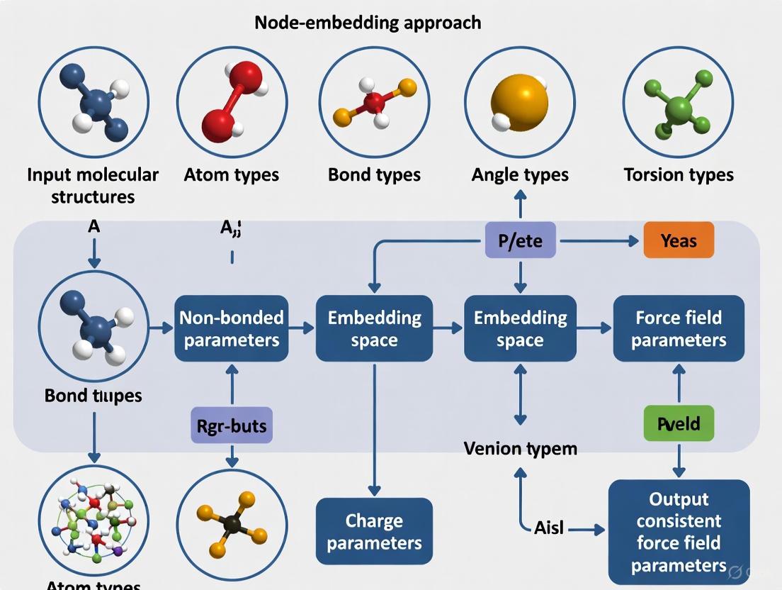
In this workflow, the 2D molecular graph ( G(V, E) ), where ( V ) represents atoms (nodes) and ( E ) represents bonds (edges), serves as the sole input. The core innovation is the use of a graph attentional neural network to generate a continuous, high-dimensional embedding (or feature vector) for each atom [14]: [ \nui = \text{GNN}(G) ] These atom embeddings ( \nui ) encode the chemical environment of each atom based on the molecular graph. The embeddings are subsequently used to predict the full set of MM parameters ( \xi ) for all bonded interactions (bonds, angles, torsions, impropers) via a transformer model ( \psi^{(l)} ) that respects the required permutation symmetries [14]: [ \xi{ij\ldots}^{(l)} = \psi^{(l)}(\nui, \nuj, \ldots) ] This two-step process—from graph to embeddings, then embeddings to parameters—ensures that chemically equivalent atoms receive identical parameters, guaranteeing consistency. The resulting parameters define a potential energy surface that can be evaluated for any molecular conformation ( x ) using the standard MM energy function, ( E(x) = E{\text{MM}}(x, \xi) ) [14]. As the model is differentiable, it can be trained end-to-end on quantum mechanical (QM) data to predict energies and forces.
Implemented Workflows and Architectures
The Grappa Force Field
Grappa employs a graph attentional neural network followed by a symmetry-preserving transformer to predict MM parameters [14]. Its key features are:
- Input: Only the 2D molecular graph, with no need for hand-crafted chemical features.
- Symmetry Preservation: The architecture explicitly respects the permutation symmetries required for the energy contributions of bonds, angles, and torsions [14].
- Computational Efficiency: Parameters are predicted once per molecule; subsequent energy evaluations have the same cost as traditional MM force fields, enabling simulation in standard MD engines like GROMACS and OpenMM [14].
The ByteFF Force Field
ByteFF utilizes an edge-augmented, symmetry-preserving molecular graph neural network trained on a massive, diverse QM dataset [21]. Its workflow includes:
- Dataset: 2.4 million optimized molecular fragment geometries and 3.2 million torsion profiles calculated at the B3LYP-D3(BJ)/DZVP level of theory [21].
- Differentiable Loss: Incorporates a differentiable partial Hessian loss to improve the accuracy of predicted vibrational frequencies [21].
- Comprehensive Parameterization: Predicts all bonded and non-bonded parameters (van der Waals and partial charges) simultaneously for drug-like molecules [21].
Automated Pipeline for Complex Materials
For parametrizing complex systems like amino acid-based metal-organic frameworks (MOFs), a hybrid, highly automated pipeline has been developed [32]. This approach combines:
- Cluster-to-Periodic Transfer: Deriving parameters from ab initio calculations on a finite, representative cluster model and seamlessly transferring them to the periodic system [32].
- GAFF Integration: Leveraging the Generalized Amber Force Field (GAFF) for dihedral parameters and employing tools like AmberTools and MCPB for parameter mapping and metal center parametrization [32].
The following diagram illustrates the unified logical workflow from a 2D molecular graph to MD-ready simulations, encapsulating the principles of the above approaches.
Experimental Protocols
Protocol 1: Training a Node-Embedding Force Field
This protocol outlines the steps for training a model like Grappa or ByteFF.
- Objective: To train a GNN model that predicts MM force field parameters directly from 2D molecular graphs.
- Input: 2D molecular structures (e.g., as SMILES strings).
- Output: A trained model capable of assigning parameters to novel molecules.
| Step | Procedure | Critical Parameters |
|---|---|---|
| 1. Dataset Curation | Generate a diverse set of small molecules and molecular fragments. Generate conformers and compute reference QM data (energy, forces, Hessians) for each [21]. | QM method: B3LYP-D3(BJ)/DZVP; Basis Set: DZVP; Number of torsion profiles: ~3.2 million [21]. |
| 2. Model Architecture | Implement a graph neural network (e.g., graph attention) to generate atom embeddings. A downstream transformer model maps embeddings to final parameters [14]. | Embedding dimension (d): 128; Number of attention heads: 8; Interaction blocks: 3 [14]. |
| 3. Model Training | Train the model end-to-end by minimizing the loss between the MM-calculated energies/forces (using predicted parameters) and the reference QM data [14]. | Loss function: Differentiable MM energy/force/Hessian loss; Optimizer: Adam; Learning rate: 1e-3 [14] [21]. |
| 4. Validation | Validate the trained model on a held-out test set of molecules. Evaluate accuracy on torsion energy profiles, relaxed geometries, and conformational energies [21]. | Metrics: Mean Absolute Error (MAE) in energy and forces; Torsion profile RMSD [21]. |
Protocol 2: Parametrizing a Novel Molecule for MD Simulation
This protocol describes the application of a pre-trained node-embedding model to parametrize a new molecule.
- Objective: To obtain a fully parameterized system for a novel molecule using a pre-trained GNN force field.
- Input: 2D structure of the target molecule.
- Output: Complete set of MM parameters and a ready-to-simulate topology file.
| Step | Procedure | Notes |
|---|---|---|
| 1. Graph Featurization | Convert the input molecule (e.g., from a SMILES string or 2D diagram) into a featurized molecular graph. | The graph should include nodes (atoms) and edges (bonds). |
| 2. Parameter Inference | Pass the molecular graph through the pre-trained GNN model. The model outputs the bonded MM parameters (bonds, angles, dihedrals) for the molecule [14]. | This step is computationally cheap and only needs to be performed once per molecule. |
| 3. Assign Non-Bonded Parameters | Assign non-bonded parameters (van der Waals, partial charges). These can be taken from an established force field or predicted by the model if it was trained to do so [14] [21]. | For Grappa, non-bonded parameters are taken from established force fields [14]. ByteFF predicts them simultaneously [21]. |
| 4. Generate Topology File | Assemble all parameters into a topology file compatible with an MD engine (e.g., GROMACS, OpenMM, AMBER). | This file defines the molecular system for simulation. |
| 5. System Setup and Simulation | Solvate the molecule, add ions, and perform energy minimization and equilibration followed by production MD. | Standard MD setup procedures apply. |
Protocol 3: Validating Force Field Performance
This protocol provides a framework for validating the accuracy of the parameterized system.
- Objective: To assess the performance of the machine-learned force field against QM data and experimental observables.
- Input: Parameterized molecule and corresponding reference data.
| Step | Procedure | Validation Metrics |
|---|---|---|
| 1. Conformational Energy | Calculate the single-point energies of multiple conformers using the MM force field and compare to QM references [21]. | MAE of relative conformational energies (kcal/mol). |
| 2. Torsion Scans | Perform a relaxed torsion scan for key dihedral angles and compare the resulting energy profile to a high-level QM scan [21]. | Root-mean-square error (RMSE) of the torsion profile energy. |
| 3. Geometry Optimization | Optimize the molecular geometry using the MM force field and compare the resulting structure (bond lengths, angles) to the QM-optimized geometry [21]. | MAE of bond lengths (Å) and angles (degrees). |
| 4. Molecular Dynamics | Run MD simulations and compute experimental observables such as J-couplings or protein folding behavior for comparison with experimental data [14]. | Reproduction of experimental J-couplings; folding of small proteins (e.g., chignolin) [14]. |
Performance Benchmarks and Data Presentation
The following tables summarize the quantitative performance of node-embedding force fields as reported in the literature.
Table 1: Performance of Node-Embedding Force Fields on Benchmark Datasets.
| Force Field | Test System | Key Metric | Reported Performance | Reference |
|---|---|---|---|---|
| Grappa | Small Molecules, Peptides, RNA (Espaloma Benchmark) | Outperforms traditional and machine-learned (Espaloma) MM force fields [14]. | State-of-the-art MM accuracy [14]. | |
| Grappa | Peptide Dihedral Angles | Matches Amber FF19SB without requiring CMAP corrections [14]. | Closely reproduces experimental J-couplings [14]. | |
| Grappa | Small Protein (Chignolin) | Improves calculated folding free energy [14]. | Recovers experimentally determined folded structure [14]. | |
| ByteFF | Drug-like Molecules | Torsional Energy Profile RMSE | State-of-the-art performance on various benchmarks [21]. | |
| ByteFF | Drug-like Molecules | Conformational Energy MAE | Excels in predicting relaxed geometries and forces [21]. |
Table 2: Computational Efficiency Comparison.
| Method | Computational Cost for Energy Evaluation | Suitability for Large-Scale MD |
|---|---|---|
| Traditional MM (GAFF, AMBER) | Low (Baseline) | Excellent (Million-atom systems on a single GPU) [14]. |
| Node-Embedding MM (Grappa, ByteFF) | Low (Same as traditional MM) [14] | Excellent (Inherits MM efficiency; used for viruses) [14]. |
| E(3)-Equivariant MLFF | Several orders of magnitude higher than MM [14] | Limited (Requires thousands of GPUs for million-atom systems) [14]. |
The Scientist's Toolkit: Essential Research Reagents
Table 3: Key Software Tools and Resources for Node-Embedding Force Field Development and Application.
| Tool / Resource | Type | Primary Function | Relevance to Workflow |
|---|---|---|---|
| Grappa | Software Package | A machine-learned molecular mechanics force field that predicts parameters from a 2D graph [14]. | Core application for end-to-end parametrization. |
| GROMACS / OpenMM | MD Simulation Engine | High-performance software for running molecular dynamics simulations [14]. | Used to execute MD with the parameters generated by Grappa. |
| AMBER / GAFF | Force Field & Tools | A suite of programs for biomolecular MD simulation and force field parametrization [32]. | Provides a foundation for non-bonded parameters and validation; tools used in hybrid pipelines. |
| RDKit | Cheminformatics Library | Open-source toolkit for cheminformatics and molecule manipulation [21]. | Used for generating initial 3D conformations from 2D graphs during dataset creation. |
| Espaloma | Machine-Learned Force Field | A predecessor to Grappa that also uses GNNs for parameter assignment [14]. | Provides a benchmark and conceptual foundation for the node-embedding approach. |
| DPmoire | MLFF Software | A tool for constructing accurate machine learning force fields for complex moiré material systems [33]. | Demonstrates the transferability of the workflow concept to materials science. |
The accuracy of Molecular Dynamics (MD) simulations is fundamentally constrained by the underlying force fields. Traditional molecular mechanics (MM) force fields rely on fixed atom types and lookup tables for parameter assignment, which can limit their transferability and accuracy across diverse chemical environments [14]. In the context of a broader thesis on node-embedding approaches for consistent force field parameter assignment, this case study examines Grappa, a machine learning framework that leverages graph-based neural networks to predict MM parameters directly from the molecular graph [14] [34]. By replacing hand-crafted atom-typing rules with a learned, context-aware representation of chemical environments, Grappa aims to achieve state-of-the-art MM accuracy with the same computational efficiency as traditional force fields, enabling more reliable simulations of proteins and peptides [14].
Grappa's architecture is designed to be end-to-end differentiable and respects the fundamental permutation symmetries inherent to molecular mechanics. Its operation can be broken down into two primary stages.
Core Architecture: From Molecular Graph to Force Field Parameters
- Graph-Based Atom Embedding: Grappa employs a graph attentional neural network, inspired by transformer architectures, to process the 2D molecular graph. In this graph, nodes represent atoms and edges represent bonds. This network generates a d-dimensional embedding vector for each atom, which captures its chemical environment based on the molecular connectivity [14].
- Symmetry-Preserving Parameter Prediction: In the second stage, these atom embeddings are used to predict the specific MM parameters (e.g., force constants, equilibrium values) for every bonded interaction (bonds, angles, torsions, impropers) in the molecule. A key innovation of Grappa is its use of a transformer model with symmetry-preserving positional encoding to ensure the predicted parameters respect the required permutation symmetries of the MM energy function. For instance, the parameters for a bond between atom i and j must be invariant to their order: ξ^(bond)ij = ξ^(bond)ji [14].
This two-step process results in a complete set of MM parameters, ξ, for the molecule. The potential energy for any given spatial conformation, x, is then computed using the standard MM energy functional: E(x) = E_MM(x, ξ). Since the machine learning model is only used once per molecule to assign parameters, the subsequent energy evaluations are as computationally efficient as those of traditional MM force fields, allowing for seamless integration into MD engines like GROMACS and OpenMM [14] [34].
Workflow Visualization
The following diagram illustrates the complete Grappa parameterization and simulation workflow.
Application to Proteins and Peptides: Experimental Protocols and Validation
Grappa has been rigorously validated on a range of systems relevant to drug development and biochemical research, from small peptides to entire virus particles.
Performance Benchmarking
The following table summarizes Grappa's performance on key benchmarks for peptides and small molecules as reported in the literature [14].
Table 1: Summary of Grappa's Performance on Key Benchmarks
| System Category | Test Description | Key Comparative Result |
|---|---|---|
| Small Molecules, Peptides & RNA | Prediction of energies and forces on the Espaloma dataset (>14,000 molecules, >1 million conformations) [14] | Outperformed traditional MM force fields and the machine-learned Espaloma force field [14]. |
| Peptide Dihedral Landscapes | Evaluation of potential energy landscape of dihedral angles [14] | Matched the performance of Amber FF19SB (a state-of-the-art protein force field) without requiring the additional complexity of CMAP corrections [14]. |
| Experimental Validation | Reproduction of experimentally measured J-couplings [14] | Closely reproduced experimental values, demonstrating physical accuracy beyond just QM energy fitting [14]. |
| Protein Folding | Calculation of folding free energy for the small protein Chignolin [14] | Showed improvement over established force fields [14]. |
Protocol for Running an MD Simulation of a Peptide with Grappa
This protocol details the steps to parameterize a peptide and run a simulation using Grappa within the OpenMM ecosystem.
Table 2: Research Reagent Solutions for Grappa Simulations
| Item Name | Function / Description |
|---|---|
| Grappa Model Weights | Pre-trained machine learning model that predicts MM parameters from a molecular graph [14]. |
| OpenMM | A high-performance, open-source MD simulation toolkit used to evaluate energies and forces and integrate the equations of motion [14]. |
| OpenMM-Torch | An OpenMM plugin that allows the integration of PyTorch models, such as Grappa, into the simulation workflow. |
| AMBER Force Field (e.g., ff19SB) | Source for non-bonded parameters (van der Waals, charges). Grappa typically predicts only bonded parameters, relying on established force fields for non-bonded terms [14]. |
Input Preparation (Molecular Graph):
- Obtain the initial 3D structure of your peptide of interest from a database (e.g., PDB) or generate it using modeling software.
- Convert the 3D structure into a 2D molecular graph representation. This graph must define all atoms and the bonds between them. Common file formats like SDF or MOL2 inherently contain this information.
Parameterization with Grappa:
- Load the molecular graph into a scripted workflow that has access to the pre-trained Grappa model.
- Pass the graph through the Grappa model. The model will output a complete set of bonded MM parameters (bonds, angles, proper torsions, improper torsions) tailored to the specific chemical context of your peptide.
- At this stage, combine Grappa's predicted bonded parameters with non-bonded parameters (atomic partial charges, Lennard-Jones parameters) from a traditional force field like AMBER ff19SB [14].
Simulation Setup in OpenMM:
- Create an OpenMM
Systemobject representing your solvated and neutralized peptide system. - Instead of using the standard
ForceFieldobject to assign parameters, use a custom function to apply the Grappa-generated parameters (from Step 2) to the corresponding bonds, angles, and dihedrals in theSystem. - Use the
OpenMM-Torchplugin to ensure the forces are correctly calculated from the assigned parameters.
- Create an OpenMM
Energy Minimization and Equilibration:
- Perform standard energy minimization to remove any bad steric clashes.
- Run a series of equilibration simulations in the NVT and NPT ensembles to stabilize the temperature and density of the system.
Production MD and Analysis:
- Launch a production MD simulation to sample the conformational landscape of the peptide.
- Analyze the trajectory using standard tools (e.g., MDAnalysis, VMD) to compute properties of interest, such as root-mean-square deviation (RMSD), radius of gyration (Rg), secondary structure content, or interaction energies.
Case Study: Demonstrating Transferability to a Large System
To demonstrate its transferability and scalability, Grappa was used to parameterize a massive system comprising a whole virus particle. In this simulation [14]:
- The system contained one million atoms.
- The simulation was run on a single GPU.
- The performance achieved was comparable to highly optimized traditional force fields, yielding a similar number of timesteps per second.
- This highlights that Grappa inherits the computational efficiency of MM force fields, making it suitable for large-scale biomolecular simulations that are intractable for more expensive QM or E(3)-equivariant neural network methods [14].
Discussion
Advantages of the Node-Embedding Approach
Grappa's node-embedding methodology offers several key advantages for force field assignment in protein and peptide simulations:
- Elimination of Hand-Crafted Features: Unlike traditional MM force fields or earlier machine-learned force fields like Espaloma, Grappa requires no expert-defined chemical features (e.g., hybridization state, formal charge). It learns a representation of chemical environments directly from the molecular graph, reducing human bias and potential for error [14].
- Excellent Data Efficiency and Extensibility: The graph-based approach is highly data-efficient. This makes it particularly suited for exploring "uncharted regions of chemical space," as demonstrated by its successful application to peptide radicals, which are not well-covered by standard force field parameter tables [14] [34].
- Inherent Transferability: The model generalizes effectively from small molecules and peptides in its training set to much larger macromolecular assemblies, such as proteins and viruses, producing stable dynamics and recovering known folded structures [14].
Comparison with Other Machine Learning Force Fields
While other transferable ML force fields exist, such as MACE-OFF and ANI-2x, Grappa occupies a unique niche. Models like MACE-OFF are typically short-ranged and may not explicitly include long-range electrostatic interactions, though they are highly accurate for intramolecular potentials [35]. In contrast, Grappa's innovation lies not in creating a new energy functional, but in using machine learning to assign parameters to the well-established, physically interpretable, and highly efficient MM functional form. This allows it to be a "drop-in replacement" in existing MD workflows with no computational overhead [14].
Grappa represents a significant advancement in the application of node-embedding approaches for force field development. By learning to assign molecular mechanics parameters directly from the molecular graph, it achieves a compelling balance between the accuracy of machine learning and the computational efficiency and stability of traditional force fields. The case studies on peptides and proteins confirm that Grappa provides state-of-the-art accuracy for energy and force predictions, reliably reproduces experimental observables, and is fully capable of large-scale, long-timescale simulations of biologically relevant systems. Its extensibility to new chemistries, like peptide radicals, positions it as a powerful tool for researchers and drug development professionals aiming to perform more predictive molecular simulations.
Molecular dynamics (MD) simulations are a pivotal tool in computational drug discovery, providing atomic-level insights into the dynamical behaviors, physical properties, and interactions of molecular systems [36]. The accuracy and reliability of these simulations hinge on the force field—a mathematical model that describes the potential energy surface of a molecular system. Conventional molecular mechanics force fields (MMFFs) balance computational efficiency with accuracy but face significant challenges in covering the rapidly expanding synthetically accessible chemical space [37] [36].
This case study examines ByteFF, a data-driven, Amber-compatible force field developed by ByteDance Research. ByteFF represents a paradigm shift from traditional look-up table parameter assignment to a node-embedding approach using a graph neural network (GNN). This method learns to assign consistent force field parameters directly from chemical environments, enabling accurate coverage of an expansive drug-like chemical space [37] [36] [38].
The ByteFF Framework: A Node-Embedding Approach
The core innovation of ByteFF is its end-to-end differentiable force field construction. Instead of relying on manually assigned atom types and pre-determined parameter tables, ByteFF uses an edge-augmented, symmetry-preserving molecular graph neural network to perceive chemical environments and predict all bonded and non-bonded parameters simultaneously [37] [38].
Key Architectural Principles
- Graph as Input: A molecule is represented as a graph where nodes are atoms and edges are bonds. This graph structure is the foundation for the node-embedding system.
- Edge-Augmentation: The GNN incorporates both node (atom) and edge (bond) features, capturing richer contextual relationships within the molecule [38].
- Symmetry Preservation: The model is explicitly designed to maintain the chemical symmetry inherent in molecular structures. This ensures that symmetry-equivalent atoms receive identical parameters, guaranteeing physically correct behavior [38].
- Charge Conservation: The predicted partial charges are automatically corrected to conserve the total charge of the molecule, a critical requirement for meaningful simulations [38].
The following diagram illustrates the flow of information from a molecular graph to the final force field parameters through the GNN-based node-embedding system.
Data Foundation and Curation
The performance of any data-driven model is contingent on the quality and scale of its training data. The ByteFF project constructed a massive, diverse, and high-quality dataset from quantum mechanics (QM) calculations [37] [36] [38].
- Fragment Generation: Molecular fragments were derived from the ChEMBL database and the ZINC20 dataset, selected for diversity based on drug-likeness (QED), topological features, and other chemical properties [38].
- Quantum Mechanical Calculations: The dataset was generated at the B3LYP-D3(BJ)/DZVP level of theory, a robust quantum chemistry method, and includes:
- 2.4 million optimized molecular fragment geometries with analytical Hessian matrices, which characterize the curvature of the potential energy surface near energy minima [37] [38].
- 3.2 million torsion profiles, representing energetic scans of dihedral angles for both non-ring and in-ring molecular fragments, crucial for capturing conformational energetics [37] [38].
Experimental Protocol: Training and Optimization
The training of the ByteFF GNN was a carefully orchestrated, multi-stage process designed to efficiently learn the complex mapping from chemical structure to force field parameters [38].
Multi-Stage Training Workflow
The training procedure was broken down into three distinct stages to ensure stable convergence and high accuracy across all parameter types.
Detailed Methodologies
Protocol 1: Pre-training for Equilibrium Parameters
- Objective: Initialize the model to predict reasonable non-bonded parameters and equilibrium geometries (bond lengths, angles).
- Input Data: 2.4 million optimized molecular fragment geometries and Hessian matrices.
- Loss Function: Mean Squared Error (MSE) against a baseline force field (GAFF-2.2) is used initially. A key innovation is the use of a differentiable partial Hessian loss, which fits force constants by comparing blocks of the predicted Hessian matrix to the QM-calculated Hessian [38]. This provides a direct, physics-informed learning signal.
- Output: A pre-trained model with a good baseline understanding of molecular structure.
Protocol 2: Focused Torsion Training
- Objective: Specialize the model in predicting accurate torsional energy profiles, which are critical for conformational sampling.
- Input Data: 3.2 million torsion profiles.
- Loss Function: A Boltzmann-weighted MSE is employed during an iterative optimization-and-training procedure. This weighting scheme focuses the model's learning on the thermally accessible energy regions of the torsion profile, which are most relevant for molecular dynamics simulations [38].
- Output: A model refined for torsional energetics.
Protocol 3: Off-Equilibrium Fine-Tuning
- Objective: Enhance the model's accuracy in predicting energies and forces for conformations that are far from energy minima, a regime critical for dynamics.
- Input Data: A smaller, purpose-built dataset of off-equilibrium molecular conformations.
- Loss Function: Standard MSE for energies and atomic forces [38].
- Output: The final ByteFF model, robust for both static and dynamic simulations.
Performance Benchmarks
ByteFF was rigorously evaluated against standard benchmark datasets and compared to traditional force fields. The following tables summarize its state-of-the-art performance.
Table 1: Performance on Geometry and Torsion Benchmarks [38]
| Benchmark Metric | Benchmark Dataset | ByteFF Performance | Competitive Force Fields |
|---|---|---|---|
| Relaxed Geometry (RMSD) | OpenFFBenchmark | Significant reduction in atomic position RMSD | GAFF, OPLS, OpenFF |
| Torsion Profile (TFD) | TorsionNet500, BDTorsion | Lower Torsion Fingerprint Deviations (TFD) | OPLS3e, OpenFF |
| Relative Conformational Energy (ΔΔE) | Internal Benchmark | Smaller relative energy differences | GAFF, OPLS, OpenFF |
Table 2: Quantitative Results on Key Torsion Types [38]
| Torsion Type | ByteFF RMSD (kcal/mol) | Legacy FF RMSD (kcal/mol) |
|---|---|---|
| In-Ring Torsions | ~1.5 | >2.0 |
| Non-Ring Torsions | ~0.7 | ~1.2 |
The Scientist's Toolkit: Essential Research Reagents
The development and application of advanced force fields like ByteFF rely on a suite of computational tools and data resources.
Table 3: Key Reagents for Data-Driven Force Field Development
| Research Reagent | Function in ByteFF Development | Relevance to the Field |
|---|---|---|
| Graph Neural Network (GNN) | Core model for learning the mapping from molecular graph to parameters [37]. | Enables consistent, environment-aware parameter assignment beyond fixed atom types. |
| Quantum Chemistry Software | Used to compute the reference data (geometries, Hessians, torsion scans) at the B3LYP-D3(BJ)/DZVP level [37]. | Provides the "ground truth" data for training and benchmarking. |
| ChEMBL / ZINC20 Databases | Sources for diverse, drug-like molecular structures used in dataset generation [38]. | Ensures training data covers a pharmaceutically relevant chemical space. |
| AMBER/GAFF Functional Form | The analytical equations into which ByteFF predicts parameters [36]. | Ensures compatibility with existing MD software (e.g., AMBER, GROMACS). |
| OpenFFBenchmark & TorsionNet500 | Independent datasets used for objective performance evaluation [38]. | Provides standardized benchmarks for comparing different force fields. |
ByteFF demonstrates the transformative potential of applying a node-embedding approach to force field parameterization. By leveraging a GNN trained on a massive QM dataset, it achieves superior accuracy and expansive coverage of drug-like chemical space, addressing a critical bottleneck in traditional methods. Its state-of-the-art performance in predicting geometries, torsional profiles, and conformational energies makes ByteFF a valuable tool for computational drug discovery, from initial candidate screening to detailed binding mode analysis. This work paves the way for more robust, reliable, and automated molecular simulations.
Molecular dynamics (MD) simulations provide powerful computational tools for studying biomolecular systems, with GROMACS and OpenMM representing two widely used simulation engines. This application note details their practical integration and use, framed within a broader research thesis on a node-embedding approach for consistent force field parameter assignment. This methodology conceptualizes atoms, their types, and relationships as a graph, where topological features are embedded into a vector space to inform parameter selection. The protocols below are designed for researchers and drug development professionals requiring robust, reproducible simulation workflows.
Engine Architecture and Force Field Handling
Foundational Algorithms and Force Field Paradigms
Both GROMACS and OpenMM solve Newton's equations of motion to simulate atomic interactions over time [39] [40]. The core MD algorithm involves computing forces from a potential energy function and using a numerical integrator to update atomic positions and velocities [39]. However, they differ significantly in their architectural philosophies and force field implementation strategies.
Table: Comparison of GROMACS and OpenMM Fundamental Characteristics
| Feature | GROMACS | OpenMM |
|---|---|---|
| Primary Architecture | Standalone application with command-line tools | Library with Python API |
| Force Field Definition | Static parameter files included with distribution [41] | XML-based force field files [42] |
| Integrator Options | md (leap-frog), md-vv (velocity Verlet), sd (stochastic dynamics) [43] |
LangevinMiddleIntegrator, VerletIntegrator [44] |
| Non-bonded Handling | Verlet buffered neighbor searching with pair lists [39] | Multiple methods including PME with specified cutoffs [44] |
| Typical Workflow | Sequential command-line tools (pdb2gmx, grompp, mdrun) |
Python scripting environment |
Force Field Implementation and Parameter Assignment
The node-embedding approach for parameter assignment conceptualizes atoms as nodes and their chemical relationships as edges in a graph. Force field parameters are assigned based on atom types and classes, which can be viewed as learned embeddings in this graph structure.
In GROMACS, force fields like AMBER99SB-ILDN and CHARMM36 provide fixed parameter sets where "the combination of equations and parameters form a consistent set" [41]. The software warns that "it is in general dangerous to make ad hoc changes in a subset of parameters" due to interdependencies [41].
OpenMM uses a more flexible system where <AtomTypes> define the most specific identification of an atom, while <AtomClasses> group types that are usually treated identically [42]. Residue templates specify atoms, their types, and bonds, enabling automatic parameter assignment based on chemical context [42]. This structure aligns well with node-embedding approaches where atomic environments inform parameter selection.
Experimental Protocols
GROMACS MD Simulation Protocol
The following protocol describes a complete MD simulation workflow for GROMACS, suitable for proteins like alanine dipeptide in explicit solvent [40].
System Preparation and Topology Generation
- Structure Preparation: Obtain initial coordinates in PDB format. The PDB file provides "the initial positions of the atoms in the system" [40].
- Topology Generation: Use
pdb2gmxto generate molecular topology: This command processes the input structure, assigns force field parameters, and generates topology files including position restraints. - Box Creation and Solvation: Creates a simulation box with 1.0 nm minimum distance between the solute and box edges, then fills with water molecules.
- System Neutralization: Replaces water molecules with ions to neutralize system charge.
Energy Minimization and Equilibration
Energy Minimization:
Performs steepest descent or conjugate gradient minimization to remove steric clashes [43].
Equilibration Phases:
- NVT Equilibration (100 ps): Stabilizes temperature using thermostat like Langevin dynamics.
- NPT Equilibration (100 ps): Achieves correct density with barostat.
Production MD
- Launch Production Simulation:
Executes production MD with parameters defined in
md.mdp.
Table: Key GROMACS .mdp Parameters for Production MD
| Parameter | Recommended Value | Description |
|---|---|---|
integrator |
md or md-vv |
Leap-frog or velocity Verlet integrator [43] |
dt |
0.002 | Time step in ps (2 fs for all-atom) [40] |
nsteps |
500000 | Number of steps (1 ns for dt=0.002) |
nstxout |
5000 | Coordinate output frequency (steps) |
nstenergy |
5000 | Energy output frequency (steps) |
coulombtype |
PME |
Particle Mesh Ewald for electrostatics |
rcoulomb |
1.0 | Short-range electrostatic cut-off (nm) |
rvdw |
1.0 | van der Waals cut-off (nm) |
tcoupl |
v-rescale |
Temperature coupling algorithm |
pcoupl |
Parrinello-Rahman |
Pressure coupling algorithm |
OpenMM MD Simulation Protocol
The following protocol describes a complete Python-based MD workflow in OpenMM, implementing the same scientific goals as the GROMACS protocol but with programmatic control.
Complete Python Implementation
Advanced Features: Enhanced Sampling and Performance
OpenMM enables advanced sampling techniques through its programmable interface:
Metadynamics:
GPU Acceleration with MPS: For multiple concurrent simulations, NVIDIA's Multi-Process Service improves throughput [45]:
Checkpointing for Long Simulations:
The Scientist's Toolkit: Essential Research Reagents
Table: Key Components for MD Simulations
| Component | Function | Example Sources/Formats |
|---|---|---|
| Force Fields | Defines potential energy functions and parameters | AMBER, CHARMM, GROMOS-96 [41] |
| Solvent Models | Represents water environment | TIP3P, TIP4P, SPC [44] |
| Integrators | Numerical methods to solve equations of motion | Leap-frog, Velocity Verlet, Langevin [43] |
| Thermostats | Regulates simulation temperature | Langevin, Nose-Hoover, v-rescale |
| Barostats | Controls system pressure | Parrinello-Rahman, Berendsen |
| Topology Files | Defines molecular structure and connectivity | .top (GROMACS), .prmtop (AMBER), XML (OpenMM) [42] |
| Coordinate Files | Atomic positions | .pdb, .gro, .crd |
Node-Embedding Framework for Parameter Assignment
The node-embedding approach conceptualizes force field parameterization as a graph learning problem. In this framework:
- Atoms represent nodes in a graph, with chemical bonds as edges
- Atom types and classes form the initial feature space [42]
- Graph neural networks or embedding algorithms learn low-dimensional representations that capture chemical environments
- Parameter prediction occurs in this learned space, ensuring consistency
This approach aligns with modern "graph neighbor-embedding (graph NE) frameworks that directly pull together embedding vectors of adjacent nodes" [5]. For force field development, this means parameters can be assigned based on learned similarity in chemical environment rather than manual type definitions.
Performance Optimization and Scalability
Computational Performance Considerations
Table: Performance Optimization Strategies
| Strategy | GROMACS | OpenMM |
|---|---|---|
| GPU Utilization | Built-in CUDA/OpenCL support | Native CUDA, OpenCL, CPU support |
| Multiple Simulations | Separate processes per simulation | MPS for concurrent GPU simulations [45] |
| Large Systems | Domain decomposition parallelism | Built-in particle mesh Ewald (PME) |
| Long Time Steps | Mass repartitioning (4 fs with mass-repartition-factor) [43] |
Constraint algorithms (HBonds) |
Scalable Deployment on Cloud Infrastructure
For large-scale deployment on cloud platforms like SaladCloud, implement chunked simulation workflows [46]:
This approach enables fault-tolerant execution on interruptible cloud instances by frequently saving state and adapting to node performance characteristics.
GROMACS and OpenMM provide complementary approaches to molecular dynamics simulations, with the former offering optimized production workflows and the latter enabling programmatic control and flexibility. The node-embedding framework for parameter assignment represents a promising research direction that could bridge these implementations through consistent, learning-based parameterization. The protocols detailed herein provide researchers with robust methodologies for employing these tools in drug discovery and biomolecular research.
Optimizing Performance and Troubleshooting Common Challenges in Node-Embedding FFs
Addressing Data Scarcity and Ensuring Coverage of Uncharted Chemical Space
The exploration of chemical space, the vast universe of all possible molecular structures, is fundamentally constrained by two interconnected challenges: extreme data scarcity and the limited coverage of commercially available compounds. With an estimated 10^60 drug-like molecules existing, only a minuscule fraction has been synthesized or characterized, creating significant bottlenecks in drug discovery and materials science [47]. This scarcity is particularly problematic for developing accurate machine learning models and force fields, which require extensive, high-quality data for reliable parameterization.
Modern computational approaches are now leveraging advanced node-embedding techniques and data-driven sampling strategies to address these limitations. By mapping molecular structures into continuous vector spaces, researchers can systematically identify and characterize unexplored regions of chemical space, enabling more consistent force field parameter assignment across diverse molecular architectures [5] [21]. This application note details protocols and methodologies for effectively navigating and sampling these uncharted territories to enhance force field development and compound discovery.
Mapping the Unexplored: Identifying Gaps in Chemical Space
Quantifying the Coverage Problem
Systematic analysis of commercially available chemical libraries reveals significant bias and coverage gaps. Research using self-organizing maps (SOMs) trained on 16 calculated physicochemical properties of known drugs has identified highly overrepresented regions alongside almost completely unoccupied regions that still resemble drug-like properties [48]. These underrepresented portions remain compatible with rigorous industry filters like the Rule of Five, suggesting they represent viable but neglected chemical space.
Table 1: Commercially Available Compound Coverage Analysis
| Analysis Method | Dataset Size | Key Finding | Reference |
|---|---|---|---|
| Self-Organizing Maps (SOM) | 16 physicochemical properties | Identified highly overrepresented and unoccupied drug-like regions | [48] |
| Recurrent Neural Networks | 448 CDK4 inhibitors, 453 Pim1 inhibitors | Discovered novel kinase inhibitors beyond training data | [47] |
| Evolutionary Algorithms + CSP | 20 benchmark molecules | Located optimal materials by exploring unpromising molecular regions | [49] |
Node Embedding for Chemical Space Representation
Node embedding approaches have emerged as powerful tools for mapping chemical space into continuous representations that preserve molecular relationships. The graph neighbor-embedding (graph NE) framework directly pulls together embedding vectors of adjacent nodes without relying on random walks, strongly outperforming state-of-the-art algorithms like DeepWalk and node2vec in local structure preservation [5]. These embeddings create a continuous, navigable space where molecular similarity and diversity can be quantitatively assessed.
Protocols for Expanding Chemical Space Coverage
Data-Driven Force Field Parameterization
The ByteFF protocol represents a comprehensive approach to force field development that addresses data scarcity through expansive dataset construction and machine learning:
Table 2: ByteFF Force Field Development Protocol
| Stage | Procedure | Output | Application |
|---|---|---|---|
| Dataset Construction | Fragment molecules from ChEMBL/ZINC20; Generate 2.4M optimized geometries and 3.2M torsion profiles at B3LYP-D3(BJ)/DZVP level | Diverse molecular fragments with QM properties | Training set for force field parameterization [21] |
| Model Architecture | Edge-augmented, symmetry-preserving molecular graph neural network (GNN) | Prediction of bonded/non-bonded parameters | Transferable parameter assignment across chemical space |
| Validation | Benchmark on relaxed geometries, torsional profiles, conformational energies | State-of-the-art accuracy across diverse molecular sets | Confirmation of chemical space coverage |
Crystal Structure Prediction-Informed Evolutionary Optimization
For materials discovery, incorporating crystal structure prediction (CSP) into evolutionary algorithms enables identification of promising molecules with favorable solid-state properties:
Protocol Steps:
- Initial Population Generation: Create diverse set of candidate molecules from available building blocks
- Fitness Evaluation: Perform automated crystal structure prediction using efficient sampling schemes (e.g., Sampling A: 5 space groups, 2000 structures each)
- Selection: Rank molecules by target property (e.g., charge carrier mobility) in predicted crystal structures
- Genetic Operations: Apply crossover and mutation to create new candidate molecules
- Iteration: Repeat for 50-100 generations or until convergence
This approach has been shown to outperform property-based optimization alone, discovering molecules with higher predicted electron mobilities by accounting for crystal packing effects [49].
Generative AI for Scaffold Hopping and Space Exploration
Generative models create novel molecular structures beyond existing chemical libraries:
Recurrent Neural Network Protocol:
- Training Data Curation: Collect known active molecules (e.g., 453 Pim1 inhibitors from ChEMBL)
- Transfer Learning: Pre-train on general compound collections (e.g., DrugBank), then fine-tune on target-specific molecules
- Sequence Generation: Generate novel SMILES strings using temperature sampling to control diversity
- Validation: Synthesize and test top candidates (successfully identified potent Pim1 inhibitor and CDK4 leads) [47]
Advanced models including variational autoencoders (VAEs), generative adversarial networks (GANs), and normalizing flows (NF) can navigate chemical space beyond structural constraints, enabling scaffold hopping and discovery of novel core structures while maintaining biological activity [50].
The Scientist's Toolkit: Essential Research Reagents and Solutions
Table 3: Key Research Reagents and Computational Tools
| Tool/Resource | Function | Application Note |
|---|---|---|
| Graph Neural Networks (GNNs) | Node embedding and property prediction | Preserves molecular symmetry; enables transferable parameter learning [21] [10] |
| Self-Organizing Maps (SOMs) | Chemical space visualization and gap identification | Maps 16+ physicochemical properties; identifies drug-like unexplored regions [48] |
| Evolutionary Algorithms | Global optimization in chemical space | Guided by CSP or property predictions; avoids local minima [49] |
| ByteFF Dataset | Training data for force field development | 2.4M optimized fragments + 3.2M torsion profiles at consistent QM level [21] |
| DPmoire Software | ML force field construction for moiré systems | Specialized for complex systems with limited data [33] |
| Allegro/NequIP Frameworks | Machine learning force field training | Achieves meV/atom accuracy required for sensitive electronic properties [33] |
Discussion and Future Perspectives
The integration of node-embedding approaches with data sampling strategies creates a powerful framework for addressing chemical space coverage challenges. The graph neighbor-embedding framework provides a mathematically rigorous foundation for representing molecular similarity, enabling consistent parameter assignment across diverse chemical structures [5]. When combined with the expansive dataset construction exemplified by ByteFF, these approaches significantly mitigate the data scarcity problem in force field development [21].
Future directions include developing multimodal representation learning that integrates structural, physicochemical, and bioactivity data, and creating better benchmarks for assessing chemical space coverage [10]. As generative models evolve, interactive exploration of chemical space will enable more efficient navigation toward regions with desired properties while ensuring novelty [51]. The continued refinement of automated force field parameterization using graph neural networks will be crucial for extending accurate molecular simulations to currently uncharted chemical territories.
These protocols and tools collectively address the fundamental challenge of data scarcity in chemical space exploration, enabling more systematic discovery of functional molecules and materials while ensuring consistent parameterization across diverse molecular architectures.
Strategies for Handling Nonbonded Interactions and Long-Range Electrostatics
Accurate modeling of nonbonded interactions, including van der Waals forces and long-range electrostatics, is a cornerstone of reliable molecular simulations in drug discovery and materials science. These interactions, though typically weaker than covalent bonds, critically govern structure, dynamics, and emergent phenomena in molecular systems, from protein-ligand binding to supramolecular assembly [52]. The central challenge lies in capturing their subtle energetics and long-range character with sufficient fidelity while maintaining computational tractability for large-scale simulations.
This document frames current strategies within a broader thesis on node-embedding approaches for consistent force field parameter assignment. In this context, atoms or molecular fragments can be treated as "nodes" in a graph, and their physicochemical properties—such as partial atomic charges or van der Waals parameters—are the "embeddings" to be assigned. Modern machine learning (ML) techniques, particularly graph neural networks (GNNs), are revolutionizing this paradigm by learning to generate consistent, context-aware parameters directly from atomic structures [12] [21].
Quantitative Comparison of Modern Strategies
The following table summarizes the core principles, advantages, and limitations of key contemporary strategies for handling nonbonded interactions.
Table 1: Comparison of Strategies for Handling Nonbonded and Long-Range Electrostatic Interactions
| Strategy | Core Principle | Key Advantages | Inherent Limitations |
|---|---|---|---|
| Conventional Molecular Mechanics (MM) | Uses fixed analytical forms (e.g., Lennard-Jones, Coulomb) with pre-parameterized look-up tables [53] [21]. | High computational efficiency; well-established and validated for many biological systems [21]. | Limited accuracy due to fixed functional forms; poor coverage of expansive chemical space [21]. |
| Machine Learning Force Fields (MLFFs) | Learns potential energy surfaces (PES) from quantum mechanical data using neural networks, without fixed functional forms [21]. | High accuracy; ability to capture complex, non-pairwise additive interactions [52] [21]. | High computational cost; requires large, high-quality training datasets [21]. |
| Explicit Charge Learning (e.g., 4G-HDNNP) | Neural networks predict environment-dependent atomic charges or electronegativities, used to compute electrostatics [54]. | Directly learns physically interpretable charge quantities. | Charge values are not physically observable and depend on the partitioning scheme [54]. |
| Implicit Charge Learning (e.g., LES) | Learns "latent charges" from local atomic features by fitting to energies and forces, then computes long-range interactions via Ewald summation [54]. | Does not require reference charges; learns from observable data (energy/forces); excellent accuracy [54]. | The local feature assumption lacks theoretical guarantees and may have limitations in some systems [54]. |
| Scale-Aware/Delta-Learning (e.g., Δ-sGDML) | Decouples problem into fragment-specific models (intramolecular) and a dedicated binding model (intermolecular) [52]. | Addresses force magnitude mismatch; improves fragment-level force accuracy and simulation stability [52]. | Increased model complexity; requires defining fragments for a system. |
| Node-Embedding for Parameters (e.g., Graph NE, FFiNet, ByteFF) | Uses GNNs to assign consistent force field parameters (bonded and non-bonded) to atoms (nodes) based on their chemical environment [5] [12] [21]. | Data-driven, transferable parameters; expansive chemical space coverage; preserves chemical symmetries [21]. | Quality depends on training data diversity and quantum chemistry method [21]. |
Performance Metrics of Advanced Methods
To objectively evaluate the practical efficacy of these strategies, the table below summarizes key quantitative benchmarks reported for several advanced methods.
Table 2: Reported Performance Metrics of Selected Methods
| Method | Type | Key Performance Metrics | Reference System |
|---|---|---|---|
| Latent Ewald Summation (LES) | Implicit Charge Learning | Better accuracy in energy and force predictions compared to methods that explicitly learn charges [54]. | Charged molecules, ionic liquids, electrolyte solutions, interfaces [54]. |
| ES-Screen | Electrostatics-Driven Screening | Superior enrichment (AUC, EF1%) over docking and MM-GBSA/PBSA; identified novel drug targets validated in vitro [55]. | Diverse protein targets (N=53); DUD-E benchmark set [55]. |
| Δ-sGDML | Scale-Aware MLFF | Fragment-level force error reductions of up to 70-75%; stable MD trajectories where a single global model failed (10-400 K) [52]. | Host-guest complexes (e.g., C60@buckycatcher) [52]. |
| ByteFF | Node-Embedding for MMFF | State-of-the-art accuracy for relaxed geometries, torsional profiles, and conformational energies/forces [21]. | Expansive dataset of drug-like molecules [21]. |
| Graph NE | Node-Embedding Algorithm | Strongly outperforms DeepWalk and node2vec in local structure preservation; outperforms existing graph-layout algorithms in 2D [5]. | Non-parametric graph representation learning [5]. |
Detailed Experimental Protocols
Protocol: Electrostatics-Driven Virtual Screening with ES-Screen
ES-Screen is a unique virtual screening method that prioritizes molecules based on electrostatic complementarity, independent of molecular docking [55].
Workflow Overview:
Diagram Title: ES-Screen Virtual Screening Workflow
Step-by-Step Procedure:
Input Preparation:
- Obtain a high-resolution protein-ligand co-crystal structure (e.g., from the PDB).
- Prepare the protein structure by adding hydrogens, assigning correct protonation states, and optimizing hydrogen bonds using standard molecular modeling software.
Knowledge-Based Pharmacophore Generation:
- Derive a pharmacophore model from the co-crystallized reference (cognate) ligand. This model captures essential steric and electronic features (e.g., hydrogen bond donors/acceptors, hydrophobic regions, excluded volumes).
- The pharmacophore is used for initial pose generation for all query ligands, making the method independent of docking algorithms [55].
Ligand Pose Generation and Optimization:
- Generate poses for each query ligand from the screening library by aligning them to the pharmacophore model.
- Refine poses using excluded volume spheres to minimize steric clashes with the receptor.
Electrostatic Potential (ESP) Extrapolation:
- Calculate the electrostatic potential of the protein's binding site in the absence of the ligand.
- Extrapolate the pre-calculated ESP to the specific atom positions now occupied by the query ligand within the binding site [55].
Replacement Energy Calculation:
- This is the critical, novel step. For a query ligand
Qand the cognate reference ligandR, calculate the electrostatic replacement energy as:ΔE_elec = E_elec(Q) - E_elec(R)
- A negative ΔE_elec indicates the query ligand forms more favorable electrostatic interactions than the reference.
- Similarly, calculate replacement energies for hydrophobic and van der Waals interactions [55].
- This is the critical, novel step. For a query ligand
Similarity Scoring (Chemometrics):
- Calculate the shape and physicochemical similarity between each query ligand and the cognate reference ligand.
Final Z-Score Calculation and Ranking:
- Combine the normalized replacement energies and similarity scores into a final ranking Z-score. The electrostatic term is typically given preferential weighting [55].
- Rank all ligands in the screening library based on this Z-score. Ligands with the most negative scores (favorable energies) and highest similarities are prioritized as top hits.
Protocol: Parameter Assignment with a Node-Embedding MMFF (ByteFF)
This protocol details the use of a graph neural network to assign consistent molecular mechanics parameters for drug-like molecules, as exemplified by ByteFF [21].
Workflow Overview:
Diagram Title: Data-Driven Force Field Parameterization
Step-by-Step Procedure:
Dataset Construction:
- Source Molecules: Curate a highly diverse set of drug-like molecules from databases like ChEMBL and ZINC.
- Fragmentation: Use a graph-expansion algorithm to cleave molecules into smaller fragments (e.g., <70 atoms) to preserve local chemical environments and ensure transferability.
- Chemical Diversity: Expand fragments to cover various protonation states (within a physiologically relevant pKa range) to maximize chemical space coverage [21].
Quantum Mechanics (QM) Data Generation:
- Generate 3D conformations for all fragments.
- Perform QM calculations at an appropriate level of theory (e.g., B3LYP-D3(BJ)/DZVP) to create two primary datasets:
- Optimization Dataset: Geometry-optimized structures and their analytical Hessian matrices (for vibrational frequencies).
- Torsion Dataset: Scans of torsion profiles to accurately capture conformational energetics [21].
Graph Neural Network Training:
- Represent each molecule as a graph where atoms are nodes and bonds are edges.
- Train a symmetry-preserving GNN on the QM dataset. The model's task is to map the molecular graph to all relevant MM parameters:
- Bonded: Equilibrium bond lengths (
r0), angles (θ0), and associated force constants (k_r,k_θ), torsion parameters (k_φ). - Non-bonded: Van der Waals parameters (σ, ε) and partial atomic charges (
q) [21].
- Bonded: Equilibrium bond lengths (
- Employ a differentiable partial Hessian loss to ensure the MM-predicted vibrational spectra match the QM reference.
- Implement an iterative training-and-optimization procedure to refine parameters further.
Inference and Validation:
- For a new molecule, the trained GNN takes its molecular graph as input and predicts a complete set of self-consistent MM parameters.
- Validate the assigned parameters by benchmarking the predicted molecular geometries, torsion profiles, and conformational energies against held-out QM data [21].
The Scientist's Toolkit
Table 3: Essential Research Reagents and Computational Tools
| Item/Reagent | Function/Application | Relevance to Nonbonded Interactions |
|---|---|---|
| High-Quality QM Datasets | Serves as the ground truth for training and validating ML-based force fields and charge methods. | Provides accurate reference energies and forces, which are critical for learning subtle nonbonded and electrostatic effects [21]. |
| Graph Neural Networks (GNNs) | Core architecture for node-embedding approaches; maps atomic environment to properties. | Enables the prediction of context-aware, chemically consistent partial charges and LJ parameters for atoms in diverse molecules [12] [21]. |
| Ewald Summation | An analytical method for computing long-range electrostatic interactions in periodic systems. | The foundation for accurate electrostatics in MD simulations; integrated into methods like LES for MLFFs [53] [54]. |
| Poisson-Boltzmann Solver | Numerical solver for calculating electrostatic potentials in an implicit solvent model. | Used in methods like MM-PBSA to estimate solvation free energies and binding affinities, providing a more realistic treatment of electrostatics [55]. |
| Knowledge-Based Pharmacophore | A model representing steric and electronic features essential for molecular recognition. | In ES-Screen, provides the pose generation input, ensuring electrostatics are calculated on biologically relevant ligand orientations [55]. |
| DUD-E Benchmarking Set | A publicly available dataset for validating virtual screening methods, designed with minimal decoy bias. | Used to assess the performance of electrostatic and other scoring functions in enriching true active compounds [55]. |
Optimizing Computational Performance and Scaling to Large Biomolecular Systems
The application of machine learning (ML) to molecular mechanics force fields (MMFFs) represents a paradigm shift in computational chemistry and drug discovery. Traditional MMFFs rely on look-up tables with finite atom types, limiting their accuracy and transferability across expansive chemical spaces [21]. Node-embedding approaches, which use graph neural networks (GNNs) to assign consistent, context-aware force field parameters directly from molecular graphs, have emerged as a powerful solution. These methods learn complex relationships between chemical structure and physical parameters, enabling more accurate and scalable simulations [18]. However, integrating these data-driven models into production workflows for large biomolecular systems requires careful optimization of computational performance and rigorous validation. This application note details protocols for implementing and benchmarking these next-generation force fields, providing researchers with a framework for robust biomolecular simulation.
Performance Analysis of ML-Force Field Platforms
The transition from traditional to machine-learned force fields involves trade-offs between parameter accuracy, computational overhead, and scalability. The table below summarizes key characteristics of selected platforms.
Table 1: Comparison of Modern Molecular Mechanics Force Field Approaches
| Platform Name | Core Methodology | Differentiating Features | Reported Performance Advantages |
|---|---|---|---|
| ByteFF [21] | Data-driven, graph neural network (GNN) | Trained on 2.4M optimized molecular fragments and 3.2M torsion profiles; Amber-compatible. | State-of-the-art accuracy for relaxed geometries, torsional profiles, and conformational forces across diverse, drug-like chemical space. |
| Grappa [18] | Graph attentional network & transformer | Symmetry-preserving positional encoding; no hand-crafted chemical features required. | State-of-the-art MM accuracy on small molecules, peptides, and RNA; enables folding of small proteins in MD simulations. |
| Espaloma [18] | Graph neural network | Early proof-of-concept for using GNNs to assign MM parameters from molecular graphs. | Improved accuracy over traditional MMFFs; demonstrated the feasibility of the node-embedding approach. |
| FFiNet [12] | Force field-inspired neural network | Incorporates functional forms of bonded and non-bonded interactions into the attention mechanism. | High performance on molecular property prediction, including on small datasets without accurate 3D coordinates. |
| KA-GNN [56] | Kolmogorov-Arnold Network (KAN) GNN | Uses Fourier-series-based learnable functions for node embedding, message passing, and readout. | Superior prediction accuracy and computational efficiency compared to conventional GNNs on molecular benchmarks. |
Experimental Protocols for System Scaling and Validation
Protocol: Parameter Assignment for a Large Protein-Ligand Complex
This protocol outlines the steps to assign force field parameters using a node-embedding model like Grappa or ByteFF for a macromolecular system, preparing it for molecular dynamics (MD) simulation.
Materials:
- Input Structure: PDB file of the protein-ligand complex.
- Software:
Procedure:
- System Preparation:
a. Remove crystallographic water molecules and counterions if starting from a pristine structure.
b. Ensure the ligand molecule is properly parameterized. For node-embedding methods, provide the ligand as a molecular graph (e.g., SDF or MOL2 file) or a simplified molecular-input line-entry system (SMILES) string.
c. For traditional force field comparison, generate ligand parameters using tools like
antechamber(for GAFF) within theAmberToolssuite.
Topology Generation with Node-Embedding: a. Input the prepared molecular graph of the entire system (protein and ligand) into the GNN-based parameterization tool (e.g., Grappa). b. The GNN generates atom embeddings that represent local chemical environments [18]. c. The model then predicts all MM parameters (bonds, angles, dihedrals, non-bonded) simultaneously from these embeddings [21]. d. The tool outputs a topology file (e.g., a
.topfile for GROMACS) compatible with standard MD engines.Solvation and Ionization: a. Place the system in a simulation box (e.g., triclinic, dodecahedron) with a minimum 1.0 nm distance between the solute and box edge. b. Solvate the system using a water model (e.g., TIP3P, SPC/E). c. Add ions (e.g., Na⁺, Cl⁻) to neutralize the system's net charge and to achieve a desired physiological concentration (e.g., 150 mM).
Energy Minimization: a. Run a steepest descent energy minimization for 50,000 steps or until the maximum force is below a threshold (e.g., 1000 kJ/mol/nm). b. This relieves any steric clashes introduced during the system building process.
Protocol: Benchmarking Simulation Performance and Stability
This protocol describes how to quantitatively evaluate the performance and stability of simulations using ML-derived parameters compared to traditional force fields.
Materials:
- Hardware: High-performance computing (HPC) cluster with GPUs.
- Software: MD engine (GROMACS, OpenMM), analysis tools (e.g.,
gmx rms,gmx energy).
Procedure:
- System Equilibration: a. Perform a two-step equilibration in the NVT and NPT ensembles. b. For NVT, run for 100 ps while restraining heavy atom positions of the solute, gradually heating the system to the target temperature (e.g., 310 K). c. For NPT, run for 100 ps with positional restraints on solute heavy atoms, coupling the system to a pressure bath (e.g., 1 bar) to achieve the correct density.
Production MD Simulation: a. Run an unrestrained production simulation for a timescale relevant to the biological process (e.g., 100 ns to 1 µs for protein-ligand stability). b. Use a simulation timestep of 2 fs. c. Write trajectory frames to disk every 10-100 ps for analysis.
Performance and Stability Metrics: a. Computational Performance: Monitor nanoseconds of simulation per day (ns/day). Compare the performance of simulations using ML-assigned parameters versus traditional ones. The overhead should be minimal as the parameter prediction is a one-time cost [18]. b. Structural Stability: Calculate the root-mean-square deviation (RMSD) of the protein backbone and the ligand heavy atoms relative to the initial structure over the course of the simulation. A stable system will plateau at a low RMSD value. c. Force Field Accuracy: For validation against quantum mechanics (QM), calculate the error in conformational energies and forces on a benchmark dataset of small molecules or peptide fragments [21].
Workflow Visualization for ML-Force Field Application
The following diagram illustrates the end-to-end workflow for applying a node-embedding force field to a biomolecular system, from parameter assignment to analysis.
Table 2: Key Resources for Node-Embedding Force Field Research
| Resource / Reagent | Function / Description | Application Note |
|---|---|---|
| GROMACS / OpenMM [18] | High-performance molecular dynamics engines. | Grappa and other ML-FFs are compatible with these engines, providing a seamless path from parameter prediction to production simulation. |
| Grappa Model [18] | A machine-learned MM force field using graph neural networks. | Does not require hand-crafted chemical features, making it extensible to unexplored chemical spaces like radicals. |
| ByteFF Dataset [21] | A expansive QM dataset for training; includes 2.4M optimized geometries and 3.2M torsion profiles. | Provides the foundational data for training highly accurate, chemically diverse force fields. B3LYP-D3(BJ)/DZVP level of theory offers a cost-accuracy balance. |
| QM Reference Data (B3LYP-D3(BJ)/DZVP) [21] | High-level quantum mechanical calculations used as ground truth for training and validation. | Critical for benchmarking the accuracy of predicted energies, forces, and torsional profiles against a reliable standard. |
| Espaloma Benchmark [18] | A dataset containing over 14,000 molecules and more than 1 million states. | Serves as a standard benchmark for evaluating the accuracy of new machine-learned force fields on small molecules, peptides, and RNA. |
| Force Field-Inspired Neural Network (FFiNet) [12] | A GNN that explicitly incorporates force field energy terms into its architecture. | Particularly useful for tasks where data is limited, as it builds in physical prior knowledge, reducing the amount of training data required. |
Balancing Accuracy and Transferability to Prevent Overfitting
In computational drug discovery, molecular mechanics force fields (MMFFs) are fundamental to molecular dynamics (MD) simulations, which provide critical insights into dynamical behaviors, molecular interactions, and physical properties. The accuracy of these simulations hinges on the precise assignment of force field parameters—mathematical representations of the potential energy surface. Traditional parameter assignment often relies on look-up tables for specific chemical environments, facing significant challenges in accuracy and coverage within the rapidly expanding synthetically accessible chemical space. Node-embedding approaches, which learn low-dimensional vector representations of atoms or molecular fragments from graph-structured data, offer a promising pathway to consistent and data-driven parameter assignment. This paradigm must carefully balance two competing objectives: achieving high accuracy on known chemical domains while maintaining transferability across expansive and novel chemical spaces to prevent overfitting. This application note details protocols and methodologies to navigate this critical balance.
Core Concepts and Quantitative Comparisons
The Accuracy-Transferability Trade-off in Force Fields
Conventional MMFFs, such as GAFF and OPLS, utilize fixed analytical forms to ensure computational efficiency but can suffer from inaccuracies due to approximations in functional forms and parameter derivation. Machine learning force fields (MLFFs) can model complex potential energy surfaces with high accuracy but often at a high computational cost and with a risk of overfitting to their training data, limiting their transferability. Data-driven MMFFs like ByteFF represent an intermediate approach, using graph neural networks (GNNs) to predict parameters, aiming to preserve the efficiency of MMFFs while enhancing accuracy and coverage through learning from large, diverse quantum mechanics (QM) datasets [21].
Comparison of Node-Embedding Approaches for Parameter Assignment
The table below summarizes key node-embedding paradigms and their characteristics relevant to force field development.
Table 1: Node-Embedding Approaches for Molecular Graphs
| Embedding Approach | Core Methodology | Advantages for Force Fields | Potential Risks |
|---|---|---|---|
| Graph Neighbor Embedding (Graph NE) [5] | Directly pulls together embeddings of adjacent nodes without random walks. | Simplicity, strong local structure preservation, no costly hyperparameter tuning. | May struggle with long-range interactions in molecules. |
| Disentangled & Self-Explainable (DiSeNE) [57] | Ensures each embedding dimension corresponds to a distinct topological substructure. | Intrinsic interpretability; dimensions may align with chemical functional groups. | Increased model complexity; requires careful validation. |
| Contrastive Learning [58] [59] | Learns by contrasting positive pairs (e.g., similar nodes) against negative pairs. | Can leverage unlabeled data; good for capturing local and global structure. | Performance can be unstable; risk of negative transfer. |
| Masked Autoencoding (GraphMAE) [58] | Reconstructs masked node features or graph structures from corrupted inputs. | Shown to have robust cross-dataset transferability; stable pretraining signal. | Requires a meaningful feature set to reconstruct. |
Experimental Protocols for Node-Embedding-Based Force Fields
This section outlines a detailed protocol for developing and validating a transferable, node-embedding-based force field, following the workflow established by ByteFF [21].
Dataset Curation and Preprocessing
Objective: To generate a expansive, diverse, and high-quality dataset for training and evaluation. Materials: Molecular databases (e.g., ChEMBL, ZINC20), quantum chemistry software (e.g., for B3LYP-D3(BJ)/DZVP calculations), RDKit. Procedure:
- Molecular Selection: Curate an initial set of drug-like molecules from source databases based on criteria including aromatic rings, polar surface area (PSA), quantitative estimate of drug-likeness (QED), and element types.
- Fragmentation: Cleave selected molecules into smaller fragments (<70 atoms) using a graph-expansion algorithm. This preserves local chemical environments (e.g., bonds, angles, torsions) and enables scalable QM calculations.
- Protonation State Expansion: Generate various protonation states for each fragment within a physiologically relevant pKa range (e.g., 0.0 to 14.0) using tools like Epik, then deduplicate.
- Quantum Mechanics (QM) Calculation: a. Optimization Dataset: Generate initial 3D conformers for all fragments using RDKit. Perform geometry optimization and compute analytical Hessian matrices at a consistent QM level (e.g., B3LYP-D3(BJ)/DZVP) to capture energies, forces, and vibrational frequencies. b. Torsion Dataset: For a subset of fragments, conduct torsion scans by systematically rotating dihedral angles and computing single-point energies to create detailed torsion profiles. Critical Considerations: Dataset size and diversity are paramount for transferability. The final ByteFF dataset contained 2.4 million optimized fragments and 3.2 million torsion profiles [21].
Model Architecture and Training Strategy
Objective: To train a GNN that predicts all bonded and non-bonded MM parameters for a given molecule. Materials: Deep learning framework (e.g., PyTorch, TensorFlow), symmetry-preserving GNN architecture. Procedure:
- Graph Representation: Represent each molecule as a graph where nodes are atoms and edges are bonds. Initialize node (atom) and edge (bond) features using chemical descriptors.
- Model Selection: Implement an edge-augmented, symmetry-preserving GNN. This architecture is critical for ensuring predicted parameters are permutationally invariant and respect chemical symmetries (e.g., equivalent atoms in a carboxyl group receive identical parameters).
- Loss Function Design: Construct a multi-component loss function:
- Energy and Force Loss: Mean squared error (MSE) between QM and MM-predicted energies and atomic forces.
- Hessian Loss: A differentiable partial Hessian loss to ensure the model accurately captures vibrational frequencies and curvature of the potential energy surface.
- Physics Constraints: Incorporate regularization terms to enforce charge conservation.
- Iterative Training: Adopt an iterative training-and-optimization procedure. The model predicts parameters, which are used in a MM simulation; the results are compared to QM reference data, and the model is updated accordingly. This end-to-end refinement improves accuracy.
Validation and Transferability Assessment Protocol
Objective: To rigorously evaluate the model's accuracy and, more importantly, its transferability to novel molecules. Materials: Held-out test sets, external benchmark datasets (e.g., other public QM datasets). Procedure:
- Accuracy Metrics: Quantify performance on held-out test molecules using:
- Geometry Accuracy: Root mean square deviation (RMSD) of predicted relaxed geometries versus QM references.
- Torsion Profile Accuracy: MSE of torsional energy profiles.
- Conformational Energy/Force Accuracy: MSE for relative conformational energies and atomic forces.
- Transferability Tests: Evaluate the trained model on entirely external benchmark datasets that contain molecular scaffolds or functional groups not present in the training data. A significant performance drop indicates overfitting and poor transferability.
- Ablation Studies: Systematically remove components of the training strategy (e.g., the Hessian loss, iterative training) to isolate their contribution to final performance.
The Scientist's Toolkit: Research Reagent Solutions
Table 2: Essential Tools for Node-Embedding Force Field Development
| Tool / Reagent | Type | Function in Research |
|---|---|---|
| ChEMBL / ZINC20 Databases [21] | Data | Provide foundational molecular structures for building diverse training and test sets. |
| B3LYP-D3(BJ)/DZVP | Quantum Chemistry Method | A balanced QM method for generating accurate reference energies, forces, and Hessians for dataset creation. |
| RDKit | Cheminformatics | Handles molecular I/O, fragmentation, conformer generation, and feature calculation. |
| Graph Neural Network (GNN) | Model | Core architecture for learning from graph-structured molecular data and predicting parameters. |
| Differentiable Hessian Loss [21] | Algorithm | A key training loss component that ensures accurate capture of the potential energy surface curvature. |
| Multi-Component Loss Function | Framework | Combines energy, force, and Hessian errors to guide the model toward physically accurate predictions. |
| ogbn-papers100M [58] | Benchmark Dataset | A large-scale graph dataset; analogous datasets in molecules are needed for pretraining and transfer learning studies. |
| GraphMAE [58] | Algorithm | A masked autoencoder approach identified as robust for transfer learning; could be adapted for molecular pretraining. |
Mitigating Overfitting: Strategic Recommendations
Preventing overfitting is central to achieving transferability. The following strategies, visualized in the diagram below, are critical.
- Prioritize Data Diversity and Scale: The most effective guard against overfitting is a large, high-quality, and maximally diverse training dataset that broadly samples the target chemical space. The expansion of chemical space coverage in ByteFF was a direct result of its massive and diverse QM dataset [21].
- Incorporate Physical Inductive Biases: Hard-code known physical constraints into the model architecture and loss function. This includes enforcing permutational invariance, chemical symmetry, and charge conservation, and using a Hessian-based loss. This reduces the hypothesis space the model must learn, guiding it toward physically realistic solutions [21].
- Adopt Transfer-Oriented Pretraining Objectives: When considering pretraining on large-scale molecular corpora, prefer generative, reconstruction-based objectives like masked autoencoding (GraphMAE) over contrastive learning. Evidence from graph SSL benchmarks indicates that contrastive methods can lead to negative transfer, while masked autoencoding provides a more stable and transferable pretraining signal [58].
- Implement Rigorous and External Validation: Accuracy on a held-out test set from the same distribution as the training data is insufficient. Transferability must be explicitly quantified using external benchmark datasets that probe novel regions of chemical space [21].
Benchmarking Node-Embedding Force Fields: Validation Against QM and Experiment
The accuracy of molecular mechanics force fields is paramount for reliable atomistic simulations in drug discovery and materials science. Force field parameters, particularly those for torsional angles, must be optimized and validated against high-quality quantum mechanical (QM) reference data to ensure they faithfully reproduce a molecule's potential energy surface. Node-embedding approaches offer a powerful, data-driven method for consistent force field parameter assignment by automatically identifying atoms in similar chemical environments, thereby reducing manual intervention and improving transferability [20] [12]. This Application Note details the key validation metrics and experimental protocols for assessing force field performance, with a focus on torsional profiles, conformational energies, and forces, framed within the broader research on node-embedding methods.
Key Validation Metrics and Data
Validation involves quantifying the difference between force field predictions and benchmark data. The following table summarizes the primary metrics used for this purpose.
Table 1: Key Validation Metrics for Force Field Performance
| Metric Category | Specific Metric | Description | Interpretation & Target Value |
|---|---|---|---|
| Torsional Profile Accuracy | Root-Mean-Square Error (RMSE) | Measures the average deviation of the MM torsion scan energy profile from the QM reference surface. | A lower RMSE indicates better agreement. Bespoke fitting can reduce RMSE from ~1.1 kcal/mol to ~0.4 kcal/mol [60]. |
| Torsional Parameter Transferability | Assesses if parameters for a given chemical moiety work across different molecular contexts. | High errors indicate poor transferability, necessitating bespoke parameterization [60]. | |
| Conformational Energy | Ligand Strain Energy upon Binding | The energy penalty a ligand pays to adopt its bioactive conformation. | Values can range from 0 to >20 kcal/mol in crystal structures, though values above 5 kcal/mol may indicate refinement issues [61]. |
| Conformational Energy Penalty | The energy of a conformation relative to its global minimum. | Used in conformer generation; thresholds of 3-25 kcal/mol are used to ensure bioactive conformers are found [61]. | |
| Free Energy Perturbation (FEP) | Mean Unsigned Error (MUE) | Average absolute error in calculated relative binding free energies compared to experimental data. | A lower MUE indicates better predictive power. Bespoke torsions can improve MUE from 0.56 to 0.42 kcal/mol [60]. |
| R² Correlation | The coefficient of determination between calculated and experimental binding free energies. | Values closer to 1.0 indicate a stronger linear relationship. Can improve from 0.72 to 0.93 with bespoke parameters [60]. | |
| Forces | Force RMSE | The root-mean-square error of atomic forces (negative energy gradients) compared to ab initio calculations. | A direct measure of the local accuracy of the potential energy surface. Critical for molecular dynamics simulations. |
Experimental and Computational Protocols
Protocol for On-the-Fly Bespoke Torsion Parameterization
This protocol, leveraging a node-embedding approach for parameter assignment, involves several automated steps to derive molecule-specific torsion parameters [20].
Figure 1: Workflow for automated force field optimization
1. Molecule Fragmentation
- Objective: Decompose a complex organic molecule into smaller, manageable fragments containing at least one central rotatable bond (rotamer).
- Procedure: Using tools like RDKit, systematically break bonds around the target torsion, adding neighboring atoms in layers to preserve key chemical features like ring systems and functional groups. The resulting fragment ends are typically capped with methyl groups to maintain valency [20] [60].
- Node-Embedding Context: This step defines the local chemical environment that will be represented by the embedding.
2. Torsion Scan with a Fine-Tuned Potential
- Objective: Generate a high-accuracy potential energy surface for each fragment.
- Procedure: Perform a flexible torsion scan, where the dihedral angle of the rotatable bond is constrained at regular intervals (e.g., every 15°), and all other degrees of freedom (bond lengths, angles) are optimized. To avoid the computational cost of full QM calculations, this step uses a fine-tuned neural network potential (NNP) like DPA-2-TB. DPA-2-TB employs delta-learning to correct a fast semi-empirical method (GFN2-xTB), achieving high accuracy at a fraction of the computational cost [20].
3. Node-Embedding Fingerprint Assignment
- Objective: Create a unique, machine-readable identifier for the chemical environment of the torsion.
- Procedure: A graph neural network generates a numerical fingerprint (embedding) based on the molecular topology around the torsion. This replaces hand-crafted atom types or SMARTS patterns. Torsions with similar fingerprints are assumed to have similar optimal parameters, ensuring consistency across the force field [20] [12].
4. Parameter Optimization
- Objective: Find the MM dihedral parameters that best reproduce the QM/NNP torsion profile.
- Procedure: The force field parameters (e.g., dihedral force constants and phase angles) are optimized using a least-squares fitting procedure to minimize the RMSE between the MM and reference potential energy surfaces [20] [60].
5. Parameter Matching and Assignment
- Objective: Apply the newly optimized parameters to the original, full molecule.
- Procedure: The node-embedding fingerprint of the torsion in the full molecule is matched against the library of fragments with optimized parameters. The corresponding bespoke parameters are then assigned, ensuring seamless integration [20].
Protocol for Validating with Conformational Energy Analysis
This protocol assesses the physical plausibility of ligand conformations in protein-ligand crystal structures.
1. Data Set Curation
- Procedure: Select a high-quality set of protein-ligand complexes from the PDB. Prefer structures with high resolution (e.g., < 2.0 Å) and clear electron density for the ligand.
2. Reference State Determination
- Procedure: For each ligand, generate a low-energy conformational ensemble in vacuum or solvent using a conformer generator like OMEGA. Identify the global minimum energy conformation and several low-lying local minima.
3. Energy Calculation
- Procedure: Calculate the energy of the crystallographic conformation (the "bioactive conformation") using a validated force field or QM method. Also, calculate the energy of the global minimum conformation.
4. Strain Energy Calculation
- Procedure: Compute the conformational strain energy as the difference:
E_bioactive - E_global_minimum. - Interpretation: Strain energies below 3-5 kcal/mol are often considered plausible. Systematically higher energies may indicate inaccuracies in the crystal structure refinement or inherent limitations in the force field used for the analysis [61].
Protocol for Validating with Free Energy Perturbation (FEP)
FEP provides a rigorous test of a force field's ability to predict biologically relevant thermodynamic properties.
1. System Selection
- Procedure: Choose a congeneric series of ligands with experimentally measured binding affinities for a specific protein target (e.g., TYK2 inhibitors) [60].
2. Simulation Setup
- Procedure: For each ligand, set up atomistic MD simulations of the ligand free in solution and the ligand bound to the protein. Use explicit solvent models and appropriate counterions.
3. FEP Calculation
- Procedure: Use alchemical transformation pathways to morph one ligand into another in both the bound and free states. This allows for the calculation of the relative binding free energy (ΔΔG_bind) between ligand pairs.
4. Analysis and Validation
- Procedure: Compare the calculated ΔΔG_bind values to the experimental data. Key metrics include the Mean Unsigned Error (MUE) and the R² correlation coefficient. A successful force field will show a low MUE (e.g., < 1.0 kcal/mol) and a high R² (e.g., > 0.8) [60].
The Scientist's Toolkit
Table 2: Essential Research Reagents and Software Solutions
| Tool Name | Type | Primary Function | Relevance to Node-Embedding Approaches |
|---|---|---|---|
| DPA-2-TB | Neural Network Potential (NNP) | Provides high-accuracy potential energy surfaces for torsion scans rapidly. | The fine-tuned backbone for on-the-fly energy evaluations in the optimization workflow [20]. |
| OpenFF BespokeFit | Software Package | Automates the fitting of bespoke torsion parameters for Open Force Fields. | Implements a scalable framework for fragmentation, QC data generation, and parameter optimization [60]. |
| QCEngine | Computational Chemistry Executor | Provides a unified interface to run calculations across multiple quantum chemistry codes. | Used by BespokeFit to generate reference data on-the-fly from QM, semi-empirical, or ML methods [60]. |
| RDKit | Cheminformatics Library | Handles molecule fragmentation, manipulation, and SMARTS pattern matching. | Facilitates the initial fragmentation step and general molecular informatics tasks [20]. |
| Node-Embedding Similarity Metric | Algorithm | Replaces hand-crafted atom types with a learned representation of chemical environment. | The core of consistent parameter assignment; ensures chemically similar environments receive similar parameters [20]. |
| QCSubmit | Data Curation Tool | Curates, submits, and retrieves large quantum chemical datasets from QCArchive. | Helps build and manage the QM reference datasets needed for robust force field training and validation [60]. |
| FFiNet | Graph Neural Network | A force field-inspired neural network for molecular property prediction. | Demonstrates how force field concepts can guide the design of GNNs for better molecular representation [12]. |
Molecular mechanics force fields and emerging machine learning potentials are fundamental tools for simulating small molecules in drug discovery and materials science. The accuracy of these models in predicting molecular geometries and energies directly impacts the reliability of computational studies on protein-ligand binding, membrane permeation, and thermophysical properties. This application note provides a systematic performance comparison of established force fields—including the General AMBER Force Field (GAFF/GAFF2) and Optimized Potentials for Liquid Simulations (OPLS)—against the neural network potential ANI (ANAKIN-ME). Framed within research on node-embedding approaches for consistent parameter assignment, this analysis highlights the relative strengths and limitations of current parameterization methodologies, providing guidance for researchers selecting models for specific applications and informing future force field development.
A comprehensive benchmark study assessed nine force fields on a diverse set of 22,675 molecular structures of 3,271 small molecules by comparing force field-optimized geometries and conformer energies against reference quantum mechanical (QM) data [62]. The results demonstrated varying levels of accuracy across different force field families, with OPLS3e showing the best overall performance in reproducing QM geometries and energetics, closely followed by the Open Force Field Parsley (OpenFF 1.2) [62]. Established force fields such as MMFF94S and GAFF2 generally showed somewhat worse performance [62].
Table 1: Overall Performance Ranking of Small Molecule Force Fields
| Force Field | Overall Performance | Key Strengths | Notable Limitations |
|---|---|---|---|
| OPLS3e | Best | Accurate geometries and conformer energies | Commercial implementation |
| OpenFF 1.2 (Parsley) | Approaching OPLS3e | Excellent torsion profiles | Relatively new, less validated |
| CGenFF | Good balance | Reliable for drug-like molecules | - |
| GAFF/GAFF2 | Moderate | Widely adopted | Systematic errors in some geometries |
| MMFF94/MMFF94S | Moderate | Established history | Outperformed by newer FFs |
Torsional Potential Energy Surface Accuracy
For drug-like molecules containing biaryl fragments, accurate representation of torsional energy profiles is critical for predicting conformational preferences in protein-bound and solution states. A specialized benchmark evaluated force fields and neural network potentials on 88 biaryl fragments using root mean square deviation (RMSD) over the full potential energy surface and mean absolute deviation of the torsion rotational barrier height (MADB) relative to high-level CCSD(T1)* reference data [63].
Table 2: Performance on Biaryl Torsional Potential Energy Surfaces
| Model | RMSD (kcal/mol) | MADB (kcal/mol) | Relative Performance |
|---|---|---|---|
| ANI-1ccx | 0.5 ± 0.0 | 0.8 ± 0.1 | Most accurate |
| ANI-2x | 0.5 ± 0.0 | 1.0 ± 0.2 | Excellent |
| CGenFF | 0.8 ± 0.1 | 1.3 ± 0.1 | Good |
| OpenFF | 0.7 ± 0.1 | 1.3 ± 0.1 | Good |
| GAFF | 1.2 ± 0.2 | 2.6 ± 0.5 | Moderate |
| OPLS | 3.6 ± 0.3 | 3.6 ± 0.3 | Least accurate |
The study revealed that neural network potentials (ANI-1ccx and ANI-2x) were systematically more accurate and reliable than any traditional force fields, with ANI-1ccx achieving the best performance for predicting barrier heights [63]. This demonstrates the significant advantage of machine learning approaches for modeling complex torsional profiles.
Force Field Comparison for Specific Physical Properties
Different force fields exhibit varying performance when predicting specific physical properties. A study on diisopropyl ether (DIPE) membranes compared GAFF, OPLS-AA/CM1A, CHARMM36, and COMPASS force fields for their ability to reproduce experimental density, viscosity, and interfacial properties [64].
Table 3: Performance on Physical Property Prediction for Diisopropyl Ether
| Force Field | Density Prediction | Viscosity Prediction | Interfacial Properties |
|---|---|---|---|
| GAFF | Overestimates by 3-5% | Overestimates by 60-130% | - |
| OPLS-AA/CM1A | Overestimates by 3-5% | Overestimates by 60-130% | - |
| CHARMM36 | Accurate | Accurate | Accurate |
| COMPASS | Accurate | Accurate | Less accurate |
The results indicated that CHARMM36 provided the most accurate reproduction of experimental density and viscosity values, as well as interfacial tension between DIPE and water and partition coefficients in multicomponent systems [64]. This highlights the importance of force field selection for specific application domains, particularly for membrane simulations.
Geometric Differences Across Force Fields
A systematic analysis of geometric differences examined five force fields (GAFF, GAFF2, MMFF94, MMFF94S, and SMIRNOFF99Frosst) on a subset of the eMolecules database containing 2.7 million molecules [65]. The study used Torsion Fingerprint Deviation (TFD) and TanimotoCombo metrics to identify meaningful geometric differences, finding that the combination of SMIRNOFF99Frosst and GAFF2 force fields yielded the largest number of difference flags (305,582), indicating substantial parameterization differences [65]. In contrast, MMFF94 and MMFF94S showed the smallest number of difference flags (10,048), reflecting their similar parameterization heritage [65].
These geometric inconsistencies are particularly important for node-embedding parameter assignment approaches, as they highlight chemical regions where force fields disagree and where improved chemical perception methods could provide more consistent parameters.
Experimental Protocols
Standard Force Field Benchmarking Workflow
Dataset Curation
Select a diverse set of small molecules representing chemical space of interest. The OpenFF Full Optimization Benchmark 1 dataset provides 22,675 molecular structures of 3,271 small molecules with drug-like properties [62]. Ensure molecules have fewer than 50 heavy atoms for computational efficiency while maintaining chemical diversity. Filter molecules to avoid overlap between training and test sets when evaluating force fields with known training data.
Quantum Mechanical Reference Calculations
Perform geometry optimizations and energy calculations at the B3LYP-D3BJ/DZVP level of theory [62]. This method provides reasonably accurate conformational energies and geometries at moderate computational cost. For torsional benchmarks, employ higher-level methods such as CCSD(T1)* as reference for potential energy surfaces [63]. Calculate single-point energies for conformer ensembles to assess relative conformational energies.
Force Field Parameterization
For traditional force fields (GAFF, OPLS), assign parameters using their standard protocols:
- GAFF/GAFF2: Use ANTECHAMBER with AM1-BCC charges or RESP charges fit to HF/6-31G* electrostatic potential [66] [67]
- OPLS3e: Implement the ligand-specific approach with virtual sites for charge distribution [67]
- OpenFF: Apply SMIRKS-based atom typing with the SMIRNOFF specification [65] [62]
For neural network potentials (ANI), use pre-trained models (ANI-1x, ANI-2x, ANI-1ccx) without additional parameterization [68] [63].
Molecular Mechanics Geometry Optimization
Perform energy minimizations using each force field starting from the same initial structures to ensure differences are attributable to force field parameters rather than sampling variability [65]. Use convergence criteria of 0.0001 kcal/mol·Å for gradient tolerance to ensure thorough minimization. Employ the same optimization algorithm (e.g., L-BFGS) across all force fields for consistent comparisons.
Property Calculation and Comparison
Calculate key properties for comparison:
- Geometric differences: Use Torsion Fingerprint Deviation (TFD) and TanimotoCombo metrics rather than RMSD, as they are less dependent on molecular size [65]
- Conformer energies: Compute relative energies of conformer ensembles
- Torsional profiles: Perform relaxed scans for dihedral angles of interest
- Physical properties: Calculate density, viscosity, solvation free energies where applicable
Compare force field results against QM reference data using statistical metrics including root mean square deviation (RMSD), mean absolute deviation (MAD), and correlation coefficients.
Specialized Protocol for Torsional Potential Assessment
Extract 88 biaryl fragments from drug molecules to represent common torsional motifs [63]. Perform torsion scans at the B3LYP/6-31G level for each biaryl molecule, rotating the central biaryl dihedral in 15° increments [63]. Refine single-point energies at the CCSD(T1)* level of theory for higher accuracy reference data [63]. Evaluate each force field and neural network potential by computing single-point energies at each dihedral angle from the QM scans. Calculate rotational barrier heights as the energy difference between minimum and maximum on the potential energy surface. Compare force field and NNP performance using root mean square deviation (RMSD) over the full potential energy surface and mean absolute deviation of the torsion rotational barrier height (MADB) [63].
The Scientist's Toolkit
Research Reagent Solutions
Table 4: Essential Tools for Force Field Benchmarking
| Tool/Resource | Function | Application Notes |
|---|---|---|
| GAFF/GAFF2 Parameters | General small molecule force field | Use with AM1-BCC charges (ABCG2 for GAFF2) for hydration free energies [66] [67] |
| OPLS3e Parameters | Optimized for drug-like molecules | Includes virtual sites for improved electrostatics; commercial implementation [67] [62] |
| ANI-2x/ANI-1ccx | Neural network potentials | Sub-chemical accuracy for torsional profiles [63] [69] |
| OpenFF Parsley | SMIRKS-based open force field | Approaches OPLS3e accuracy for geometries/energies [62] |
| QCArchive Datasets | Reference QM data | Provides benchmark sets with QM geometries and energies [62] |
| TorsionDrive | Torsional scan data | Database of systematic torsion scans for parameter development |
| ForceBalance | Parameter optimization | Optimizes force field parameters against QM and experimental data |
| ANI Codebase | Neural network potential | Provides GPU-accelerated energy evaluations [69] |
This performance comparison reveals a evolving landscape in small molecule force field capabilities. Traditional force fields like OPLS3e and GAFF2 continue to be widely used, with OPLS3e currently demonstrating the best overall performance for geometries and energies of drug-like molecules. However, machine learning approaches like ANI show superior performance for specific properties like torsional barriers, achieving near-DFT accuracy with significantly lower computational cost than quantum methods. The emerging Open Force Field initiative is approaching the performance of established commercial force fields through improved chemical perception and parameterization methods. For researchers implementing node-embedding approaches for parameter assignment, these benchmarks highlight the importance of transferability across chemical space and accuracy across multiple property types. Future force field development should prioritize both improved chemical perception through approaches like node-embedding and more accurate functional forms that capture complex electronic effects.
The accuracy of biomolecular simulations is paramount for reliable insights into protein folding, drug design, and understanding biological function at the atomic level. Key benchmarks for this accuracy include the ability to predict a peptide's native folded structure and its dynamic conformational ensemble, often probed experimentally through NMR J-couplings. Traditional molecular mechanics (MM) force fields have advanced significantly but often face challenges in balancing the intricate energy landscapes of peptides. The emerging node-embedding approach for force field parameter assignment presents a paradigm shift. By using machine learning to derive consistent, environment-aware parameters directly from the molecular graph, this method offers a promising path to achieving unprecedented accuracy in simulating both structure and dynamics.
Force Field Paradigms and Quantitative Accuracy Assessment
Biomolecular force fields model the potential energy of a system through a combination of bonded terms (bonds, angles, dihedrals) and non-bonded terms (electrostatic and van der Waals interactions) [70]. The parameterization of these terms, especially torsional dihedrals, is critical for accurately capturing the conformational preferences of peptides. Recent efforts have leveraged automated fitting methods and quantum mechanical (QM) data to refine these parameters [70].
The table below summarizes the performance of various force field approaches against key experimental observables for peptides.
Table 1: Comparison of Force Field Performance on Peptide Folding and J-Couplings
| Force Field / Approach | Reported Performance on Peptide Folding | Reported Performance on J-Couplings | Key Features / Methodology |
|---|---|---|---|
| Grappa (ML-based MM) [3] | Recovers experimentally determined folding structures of small proteins (e.g., Chignolin); improves calculated folding free energy. | Closely reproduces experimentally measured J-couplings. | Graph neural network predicts MM parameters from molecular graph; uses established MM functional form for efficiency. |
| MACE-OFF (ML Force Field) [35] | Accurately simulates folding dynamics of Ala15 peptide; stable simulation of crambin protein. | Accurately reproduces J-coupling parameters for alanine tripeptide (Ala3) in vacuum and explicit water. | Short-range, transferable machine learning potential trained on first-principles data. |
| AMBER ff15-FB [70] | Better reproduces S2 order parameters and temperature dependence of secondary structure. | Better agreement with NMR scalar couplings. | Automated ForceBalance method fitting to QM data (RI-MP2/aug-cc-pVTZ). |
| AMBER ff15ipq [70] | Good agreement with ϕ/ψ distributions of model peptides; stable protein dynamics. | Information not specified in search results. | Implicitly polarized charges (IPolQ model) to account for solvation effects during parametrization. |
| GROMOS96 53A6, OPLS-AA/L, AMBER99SB [71] | Pronounced differences in secondary structure propensity; stability of folded peptides varies. | Information not specified in search results. | Traditional additive force fields; performance highly dependent on balance between helical and extended conformations. |
Protocols for Assessing Simulation Accuracy
To validate the accuracy of a force field, specific protocols must be followed to compare simulation results with experimental data. Below are detailed methodologies for assessing peptide folding and J-couplings.
Protocol for Peptide Folding Simulations and Analysis
This protocol outlines the steps for running molecular dynamics simulations of peptides and analyzing the results to assess folding accuracy.
Table 2: Key Research Reagents and Computational Tools for Folding Simulations
| Item Name | Function / Description |
|---|---|
| Model Peptides (e.g., Chignolin, Trp-cage, Ala15) | Small, fast-folding peptides with well-characterized experimental structures used as benchmarks [71] [35]. |
| MD Software (e.g., GROMACS, OpenMM, LAMMPS) | Highly optimized software packages to perform the molecular dynamics integration and compute energies/forces [3] [71] [35]. |
| Initial Conformations (folded and extended) | Simulations are started from both the native folded state and an unfolded, extended conformation to avoid bias and study folding pathways [71]. |
| Explicit Solvent Model (e.g., TIP3P, TIP4P, SPC) | Water molecules explicitly modeled to provide a realistic solvation environment for the peptide [71]. |
| Periodic Boundary Conditions | Simulation box that eliminates edge effects, with the solute a sufficient distance (e.g., ≥1.5 nm) from the box edges [71]. |
| Long-Range Electrostatics (PME) | Particle Mesh Ewald method for accurate calculation of electrostatic interactions beyond a cutoff distance [71]. |
Procedure:
- System Setup: Place the peptide (e.g., in a folded or extended conformation) in the center of a periodic box (e.g., truncated octahedron). Solvate the system with explicit water molecules. Add ions (e.g., Na⁺, Cl⁻) to neutralize the system's net charge and achieve a desired ionic strength [71].
- Energy Minimization: Perform an energy minimization (e.g., using the steepest descent algorithm) to remove any steric clashes and relax the initial structure.
- Equilibration: Run short simulations in the NVT (constant Number, Volume, Temperature) and NPT (constant Number, Pressure, Temperature) ensembles to stabilize the system's temperature and density. Apply position restraints on the peptide heavy atoms during initial equilibration to allow the solvent to relax around the solute.
- Production MD: Run a long, unbiased molecular dynamics simulation in the NPT ensemble. The length of the simulation must be sufficient to observe multiple folding and unfolding events for the peptide under study (from hundreds of nanoseconds to microseconds for small peptides) [71] [35].
- Trajectory Analysis:
- Root Mean Square Deviation (RMSD): Calculate the backbone RMSD of the simulation frames relative to the known experimental structure to assess structural stability.
- Root Mean Square Fluctuation (RMSF): Compute per-residue RMSF to analyze flexibility.
- Free Energy Surface (FES): Construct a 2D free energy surface as a function of reaction coordinates like the radius of gyration (Rg) and RMSD. The global minimum on the FES should correspond to the native folded state [35].
- Secondary Structure Analysis: Use tools like DSSP or STRIDE to assign secondary structure elements (α-helix, β-sheet) over time and calculate their propensity.
Protocol for Calculating and Validating J-Couplings
J-couplings (scalar spin-spin couplings) measured via NMR are sensitive probes of dihedral angles and provide a quantitative metric for validating a force field's description of the conformational ensemble.
Procedure:
- Conformational Sampling: Use an MD simulation trajectory of the peptide in explicit solvent, as described in Section 3.1.
- Trajectory Extraction: Save snapshots of the peptide's coordinates at regular intervals from the production trajectory. Ensure all snapshots are appropriately aligned (e.g, on the backbone heavy atoms).
- Dihedral Angle Calculation: For each snapshot, calculate the relevant dihedral angles (e.g., backbone φ and ψ angles) for all residues.
- J-Coupling Computation: Apply an empirical Karplus equation to translate the dihedral angles into predicted J-coupling values. A generic Karplus equation has the form: ( J(\theta) = A \cos^2(\theta) + B \cos(\theta) + C ) where ( \theta ) is the dihedral angle, and A, B, and C are empirically derived parameters specific to the type of J-coupling (e.g., (^3J_{\text{HNHA}}) for backbone torsion) [70].
- Ensemble Averaging and Validation: Calculate the average J-coupling value for each measured pair across the entire simulation ensemble. Compare the simulation-derived ensemble averages directly to the experimental NMR values. Statistical measures like the Pearson correlation coefficient (R) and the root mean square error (RMSE) between calculated and experimental values quantify the force field's accuracy [3] [35].
The Node-Embedding Approach for Consistent Parameter Assignment
Traditional force fields rely on a finite set of atom types and lookup tables for parameter assignment, which can lack transferability to novel chemical environments [3]. The node-embedding approach, exemplified by force fields like Grappa, overcomes this by using machine learning to predict molecular mechanics (MM) parameters directly from the molecular graph [3].
In this framework, a graph attentional neural network first generates a d-dimensional embedding vector for each atom, representing its chemical environment based on the molecular graph (atoms as nodes, bonds as edges). Subsequently, a symmetric transformer network maps the embeddings of the atoms involved in a specific interaction (bond, angle, torsion) to the corresponding MM parameters (force constants, equilibrium values). This process respects the inherent permutation symmetries of the MM energy function [3]. The entire workflow, from molecular graph to validated simulation, is depicted below.
Diagram 1: Node-embedding force field parameterization and validation workflow.
This approach is highly data-efficient and generates parameters that are intrinsically consistent with the molecular structure. Because the machine learning model is only used to assign parameters once per molecule, the subsequent molecular dynamics simulations retain the high computational efficiency of traditional MM force fields, enabling the simulation of large systems like entire virus particles [3]. The key advantage is the creation of a continuous and context-aware parameter space, moving beyond discrete atom typing and leading to improved accuracy across diverse chemical environments, including challenging systems like peptide radicals [3].
Predicting condensed-phase properties such as lattice energies and liquid densities is a fundamental challenge in computational chemistry and materials science, with critical applications in drug development and molecular design. Accurate predictions ensure the stability of solid formulations and the accuracy of solvation models, directly impacting the efficacy and development timeline of new therapeutics. This application note details modern computational methodologies that leverage machine learning (ML) and node-embedding approaches to overcome the limitations of traditional, often labor-intensive, parameter assignment methods. By framing these techniques within a broader research context of consistent, graph-based force field parameterization, we provide scientists with protocols to achieve high-accuracy predictions for complex systems.
Computational Frameworks and Data Presentation
Several modern computational frameworks have been developed to predict condensed-phase properties and force field parameters with high accuracy. The table below summarizes the core approaches, their methodologies, and reported performance.
Table 1: Computational Frameworks for Predicting Condensed-Phase Properties and Force Field Parameters
| Framework Name | Core Methodology | Target Properties / Parameters | Reported Advantages |
|---|---|---|---|
| GIPF Approach [72] | Statistical analysis of molecular surface electrostatic potentials. | Lattice energies, heats of vaporization/sublimation, liquid and crystal densities, critical constants. | Provides physical insight into noncovalent interactions; Good accuracy for macroscopic properties. |
| Grappa [14] | Graph attentional neural network + transformer to predict MM parameters directly from molecular graph. | Bond, angle, and dihedral force constants; equilibrium bond lengths and angles. | State-of-the-art MM accuracy; high computational efficiency; transferable to proteins and viruses. |
| FFiNet [12] | Force field-inspired neural network incorporating functional forms of bonded and nonbonded interactions. | Molecular properties (esp. on small datasets without accurate 3D information); protein-ligand binding affinity. | State-of-the-art performance on molecular property benchmarks; less sensitive to spatial inaccuracy. |
| SALTED [73] | Symmetry-adapted Gaussian process regression to predict electron densities in an atom-centered basis. | Electron densities; derived properties (energies, dipoles) for metals, semiconductors, and molecular crystals. | Errors of tens of meV/atom for derived energies; transferable from small to large systems (4 to 512 molecules). |
| Δ-MLP (for Water) [74] | Machine-learning potential correcting a baseline model (e.g., DFT) to coupled cluster [CCSD(T)] accuracy. | Liquid water density (including maximum), radial distribution functions, transport properties. | Agreement with experiment for structural and transport properties, including density under constant pressure. |
Quantitative benchmarks for these methods demonstrate their significant advancements. The Grappa force field, for instance, has been shown to outperform traditional molecular mechanics force fields and other machine-learned equivalents on a dataset of over 14,000 molecules [14]. The SALTED method achieves remarkable transferability, where a model trained on ice unit cells of only 4 water molecules can accurately predict the electron densities and derived energies of supercells containing up to 512 molecules with no loss of accuracy [73]. For liquid water, the Δ-MLP approach successfully reproduces the experimentally observed density maximum, a key thermodynamic property that has been challenging for many density functional theory (DFT) models [74].
Experimental and Computational Protocols
Protocol: Predicting Lattice Energies using the GIPF Approach
The General Interaction Properties Function (GIPF) approach posits that properties dependent on noncovalent interactions can be expressed accurately using quantities derived from a molecule's surface electrostatic potential [72].
- Molecular Wavefunction Calculation: Perform an ab initio quantum chemical calculation (e.g., Hartree-Fock or DFT) on the isolated molecule of interest in the gas phase to obtain its electron density.
- Molecular Surface Definition: Define the molecular surface, typically using an electron density isosurface (e.g., the 0.001 au boundary).
- Electrostatic Potential (ESP) Mapping: Calculate the electrostatic potential, V(r), at a large number of points on the molecular surface. The potential is computed as V(r) = Σ[ZA/|RA - r|] - ∫[ρ(r')/|r' - r|]dr', where ZA is the charge of nucleus A at position RA and ρ(r) is the electron density.
- Statistical Characterization: Compute a set of statistical quantities that describe the mapped ESP, including:
- The positive and negative surface potentials (VS^+ and VS^-)
- The average deviation of the positive and negative potentials (Π and Σ)
- The total variance (σ_tot^2)
- The degree of balance between positive and negative potentials (ν)
- The molecular surface area
- Application of Analytical Relationship: Input the calculated statistical descriptors into the pre-derived analytical relationship for the target property. For example, the lattice energy of a molecular crystal can be calculated using a linear function of these statistical quantities. The coefficients of this function are determined a priori by regression against a training set of molecules with known experimental lattice energies.
Protocol: Parameterizing a Machine Learning Force Field with Grappa
Grappa generates a complete set of molecular mechanics (MM) parameters for a molecule directly from its 2D graph structure, enabling accurate energy and force evaluations [14].
- Input Featurization: Represent the molecule as a graph G=(V,E), where nodes (atoms) are initially featurized using basic atomic properties (e.g., atom type, formal charge). No hand-crafted chemical features are required.
- Atom Embedding Generation: Process the molecular graph through a graph attentional neural network. This network creates a d-dimensional embedding vector for each atom that encodes its chemical environment.
- MM Parameter Prediction: For each specific interaction (bond, angle, torsion, improper dihedral), feed the embeddings of the involved atoms into a dedicated transformer module, ψ(l). This module is designed to be invariant to the permutations of atoms that leave the energy contribution unchanged (e.g., ξ^(bond)ij = ξ^(bond)ji).
- Energy Evaluation: The predicted parameters (force constants, equilibrium values) define the force field. The potential energy for any molecular conformation x is then computed using the standard MM energy function: E(x) = E_MM(x, ξ). This step can be performed in standard MD packages like GROMACS or OpenMM.
- Model Training (End-to-End): The entire Grappa model is trained end-to-end. The loss function minimizes the difference between the energies and forces predicted by the Grappa-parameterized MM force field and the reference quantum mechanical (QM) energies and forces for a diverse set of molecular conformations.
Protocol: Achieving CCSD(T) Accuracy for Liquid Densities via Δ-Learning
This protocol uses delta-learning to create a machine learning potential (MLP) for liquid water at the "gold standard" CCSD(T) level of theory, enabling accurate prediction of liquid density [74].
- Generate Baseline MD Trajectory: Perform a molecular dynamics simulation using a baseline MLP trained on a affordable level of theory, such as DFT or MP2. This generates an ensemble of diverse molecular configurations (clusters or periodic boxes) representative of the condensed phase.
- Compute High-Level Energy Corrections: For a subset of configurations from the baseline trajectory, compute the accurate energy difference, ΔE = E_CCSD(T) - E_baseline. This step is computationally intensive but is only performed on a limited dataset.
- Train the Δ-MLP: Train a second machine learning model (the Δ-MLP) to predict the energy correction ΔE as a function of the atomic structure.
- Create the Composite Model: The final model's total energy for any configuration is given by E_total = E_baseline_MLP + E_Δ-MLP.
- Run Constant-Pressure Simulations: Use the composite model to run isothermal-isobaric (NPT) molecular dynamics simulations. These simulations allow the cell volume to fluctuate, making it possible to directly compute the equilibrium density of the liquid at a given temperature and pressure.
Workflow Visualization
The following diagram illustrates the logical workflow for the Grappa force field parameterization and the Δ-learning approach for liquid properties, highlighting the integration of node-embedding concepts.
The Scientist's Toolkit
Table 2: Essential Research Reagents and Computational Tools
| Item / Software | Function in Research |
|---|---|
| Graph Neural Network (GNN) | Core architecture for learning from molecular graphs; generates atom embeddings for parameter prediction [14] [12]. |
| Transformer Module | Neural network component that processes atom embeddings to predict specific MM parameters while respecting physical permutation symmetries [14]. |
| Molecular Dynamics (MD) Engine | Software (e.g., GROMACS, OpenMM) that performs simulations using the predicted parameters to compute condensed-phase properties and trajectories [14]. |
| Quantum Chemistry Code | Software (e.g., ORCA, Gaussian) to generate reference data (energies, forces, electrostatic potentials) for model training or validation [72] [74]. |
| Resolution of the Identity (RI) Basis | A set of atom-centered basis functions used to represent the electron density for machine learning, applicable to both finite and periodic systems [73]. |
| Delta-Learning (Δ-MLP) Strategy | A technique to train a model on the energy difference between a high-accuracy and a lower-level method, making high-fidelity simulations computationally feasible [74]. |
Conclusion
Node-embedding approaches represent a paradigm shift in force field development, directly addressing the critical challenge of parameter consistency and transferability across diverse molecular systems. By learning chemically intuitive representations from data, methods like Grappa and ByteFF move beyond the limitations of discrete atom types, enabling more accurate and automated parameterization for drug-like molecules and complex biomolecules. The successful application of these force fields in reproducing quantum mechanical energies, simulating peptide folding, and predicting experimental observables underscores their robust physical basis. Future directions will likely focus on the seamless integration of explicit polarization, improved handling of long-range interactions, and expansion into new chemical territories such as metalloenzymes and covalent inhibitors. These advancements promise to make molecular simulations an even more reliable and predictive tool in rational drug design and the understanding of biological mechanisms at an atomic level.
References
- 1. Review The continuous evolution of biomolecular force fields [https://www.sciencedirect.com/science/article/abs/pii/S0969212625001911]
- 2. Data-Driven Parametrization of Molecular Mechanics Force ... [https://arxiv.org/html/2408.12817v1]
- 3. Grappa – a machine learned molecular mechanics force field [https://pmc.ncbi.nlm.nih.gov/articles/PMC11734696/]
- 4. Implementing reactivity in molecular dynamics simulations ... [https://www.nature.com/articles/s41467-024-50793-0]
- 5. Node Embeddings via Neighbor Embeddings [https://arxiv.org/html/2503.23822v2]
- 6. Node embeddings for Beginners [https://medium.com/data-science/node-embeddings-for-beginners-554ab1625d98]
- 7. Understanding Node Embeddings in Graphs: Part 5 of X ... [https://www.linkedin.com/pulse/understanding-node-embeddings-graphs-part-5-x-my-notes-ajay-taneja-1f0jf]
- 8. Group graph: a molecular graph representation with ... [https://jcheminf.biomedcentral.com/articles/10.1186/s13321-024-00933-x]
- 9. Molecular representation learning: cross-domain foundations ... [https://pubs.rsc.org/en/content/articlehtml/2025/dd/d5dd00170f]
- 10. Recent advances in molecular representation methods and ... [https://www.nature.com/articles/s44386-025-00017-2]
- 11. A Method For Predicting Molecular Point Group Based On ... [https://www.sciencedirect.com/science/article/pii/S2949747725000144]
- 12. Force field-inspired molecular representation learning for ... [https://pmc.ncbi.nlm.nih.gov/articles/PMC9901163/]
- 13. Node embedding with node2vec [https://bio-protocol.org/exchange/minidetail?id=18633648&type=30]
- 14. Grappa – a machine learned molecular mechanics force field [https://pubs.rsc.org/en/content/articlehtml/2025/sc/d4sc05465b]
- 15. Rapid parameterization of small molecules using the Force ... [https://pmc.ncbi.nlm.nih.gov/articles/PMC3874408/]
- 16. forcefield parameterization — Publications [https://www.choderalab.org/publications/tag/forcefield+parameterization]
- 17. Symmetry-invariant quantum machine learning force fields [https://pennylane.ai/qml/demos/tutorial_eqnn_force_field]
- 18. A Machine Learned Molecular Mechanics Force Field [https://arxiv.org/html/2404.00050v1]
- 19. FreeCG: Free the Design Space of Clebsch-Gordan ... [https://openreview.net/forum?id=sfi2j1Ot6j]
- 20. Efficient and Precise Force Field Optimization for ... [https://arxiv.org/html/2406.09817v1]
- 21. Data-driven parametrization of molecular mechanics force ... [https://pubs.rsc.org/en/content/articlehtml/2025/sc/d4sc06640e]
- 22. QM7 dataset [https://quantum-machine.org/datasets/]
- 23. The Largest Curated Crystal Structure Database [https://www.ccdc.cam.ac.uk/solutions/software/csd/]
- 24. Crystal structure generation with autoregressive large ... [https://www.nature.com/articles/s41467-024-54639-7]
- 25. Graph Neural Networks as a Substitute for Transformers in ... [https://arxiv.org/html/2507.04125v1]
- 26. graph-based transformer versus GNN models - PMC [https://pmc.ncbi.nlm.nih.gov/articles/PMC12100853/]
- 27. ApproxGNN: A Pretrained GNN for Parameter Prediction in ... [https://arxiv.org/html/2507.16379v1]
- 28. Drug discovery and mechanism prediction with explainable ... [https://www.nature.com/articles/s41598-024-83090-3]
- 29. Research on GNNs with stable learning | Scientific Reports [https://www.nature.com/articles/s41598-025-12840-8]
- 30. A review of transformer models in drug discovery and beyond [https://www.sciencedirect.com/science/article/pii/S2095177924001783]
- 31. Sequence-based virtual screening using transformers [https://www.nature.com/articles/s41467-025-61833-8]
- 32. Automated force field parametrization for amino acid-based ... [https://www.sciencedirect.com/science/article/abs/pii/S0927025625007062]
- 33. DPmoire: a tool for constructing accurate machine learning ... [https://www.nature.com/articles/s41524-025-01740-0]
- 34. Grappa -- A Machine Learned Molecular Mechanics Force ... [https://arxiv.org/abs/2404.00050]
- 35. MACE-OFF: Short Range Transferable Machine Learning ... [https://arxiv.org/html/2312.15211v5]
- 36. Data-Driven Parametrization of Molecular Mechanics Force ... [https://arxiv.org/html/2408.12817v2]
- 37. Data-driven parametrization of molecular mechanics force ... [https://pubs.rsc.org/en/content/articlelanding/2025/sc/d4sc06640e]
- 38. [Literature Review] Data-Driven Parametrization of ... [https://www.themoonlight.io/en/review/data-driven-parametrization-of-molecular-mechanics-force-fields-for-expansive-chemical-space-coverage]
- 39. Molecular Dynamics - GROMACS 2025.4 documentation [https://manual.gromacs.org/documentation/current/reference-manual/algorithms/molecular-dynamics.html]
- 40. Computational BioPhysics Tutorials - 2025/2026 [https://cbp-unitn.gitlab.io/QCB/tutorial2_gromacs.html]
- 41. Force field - GROMACS 2025.3 documentation [https://manual.gromacs.org/documentation/2025.3/reference-manual/functions/force-field.html]
- 42. 7. Creating Force Fields [https://docs.openmm.org/latest/userguide/application/06_creating_ffs.html]
- 43. Molecular dynamics parameters (.mdp options) [https://manual.gromacs.org/2025-rc/user-guide/mdp-options.html]
- 44. 3. Running Simulations [https://docs.openmm.org/latest/userguide/application/02_running_sims.html]
- 45. Maximizing OpenMM Molecular Dynamics Throughput with ... [https://developer.nvidia.com/blog/maximizing-openmm-molecular-dynamics-throughput-with-nvidia-multi-process-service/]
- 46. Run OpenMM on SaladCloud [https://docs.salad.com/container-engine/how-to-guides/molecular-dynamics-simulation/openmm-srcg]
- 47. Chemical space exploration based on recurrent neural networks [https://jcheminf.biomedcentral.com/articles/10.1186/s13321-020-00446-3]
- 48. Analysis of the uncharted, druglike property space by self ... [https://pmc.ncbi.nlm.nih.gov/articles/PMC9532340/]
- 49. Exploring organic chemical space for materials discovery ... [https://www.nature.com/articles/s41467-025-65564-8]
- 50. Navigating the frontier of drug-like chemical space with ... [https://www.sciencedirect.com/science/article/pii/S1359644624002587]
- 51. Chemical space visual navigation in the era of deep ... [https://www.sciencedirect.com/science/article/pii/S1359644625001059]
- 52. Delta–learned force fields for nonbonded interactions [https://arxiv.org/html/2511.01913v1]
- 53. Non-bonded interactions - GROMACS 2025.4 documentation [https://manual.gromacs.org/documentation/current/reference-manual/functions/nonbonded-interactions.html]
- 54. Machine learning of charges and long-range interactions ... [https://www.nature.com/articles/s41467-025-63852-x]
- 55. ES-Screen: A Novel Electrostatics-Driven Method for Drug ... [https://pmc.ncbi.nlm.nih.gov/articles/PMC9736079/]
- 56. Kolmogorov–Arnold graph neural networks for molecular ... [https://www.nature.com/articles/s42256-025-01087-7]
- 57. Disentangled and Self-Explainable Node Representation ... [https://arxiv.org/html/2410.21043v2]
- 58. A Benchmark Study on the Transferability of Graph Self ... [https://arxiv.org/html/2509.06975v1]
- 59. Multi-grained contrastive-learning driven MLPs for node ... [https://www.nature.com/articles/s41598-025-19189-y]
- 60. Open Force Field BespokeFit: Automating Bespoke Torsion ... [https://pmc.ncbi.nlm.nih.gov/articles/PMC9709916/]
- 61. Conformational energy range of ligands in protein crystal ... [https://pmc.ncbi.nlm.nih.gov/articles/PMC5553890/]
- 62. Benchmark assessment of molecular geometries and... [https://f1000research.com/articles/9-1390]
- 63. Benchmarking Force Field and the ANI Neural Network ... [https://pubmed.ncbi.nlm.nih.gov/33263401/]
- 64. Force field comparison for molecular dynamics simulations ... [https://www.sciencedirect.com/science/article/abs/pii/S0167732224024061]
- 65. Improving Small Molecule Force Fields by Identifying and ... [https://pmc.ncbi.nlm.nih.gov/articles/PMC8162916/]
- 66. A fast and high-quality charge model for the next generation ... [https://pmc.ncbi.nlm.nih.gov/articles/PMC7728379/]
- 67. Recent progress in general force fields of small molecules [https://www.sciencedirect.com/science/article/abs/pii/S0959440X21001603]
- 68. ANI neural network potentials for small molecule p K ... [https://pubs.rsc.org/en/content/articlehtml/2024/cp/d4cp01982b]
- 69. ANI-1: an extensible neural network potential with DFT ... [https://pmc.ncbi.nlm.nih.gov/articles/PMC5414547/]
- 70. Integration of experimental data and use of automated ... [https://www.nature.com/articles/s42004-022-00653-z]
- 71. Secondary Structure Propensities in Peptide Folding ... [https://pmc.ncbi.nlm.nih.gov/articles/PMC2711344/]
- 72. Computational prediction of condensed phase properties ... [https://www.sciencedirect.com/science/article/abs/pii/S0378381201004630]
- 73. Learning Electron Densities in the Condensed Phase - PMC [https://pmc.ncbi.nlm.nih.gov/articles/PMC8582255/]
- 74. Towards Routine Condensed Phase Simulations with ... [https://arxiv.org/html/2508.13391v1]