Molecular Dynamics vs. Monte Carlo Simulations: A Comprehensive Guide for Computational Drug Discovery
This article provides a comparative analysis of Molecular Dynamics (MD) and Monte Carlo (MC) simulation methods, tailored for researchers and professionals in drug development.
Molecular Dynamics vs. Monte Carlo Simulations: A Comprehensive Guide for Computational Drug Discovery
Abstract
This article provides a comparative analysis of Molecular Dynamics (MD) and Monte Carlo (MC) simulation methods, tailored for researchers and professionals in drug development. It covers the foundational principles of both deterministic MD and probabilistic MC approaches, explores their methodological workflows and specific applications in biomolecular modeling and drug optimization, addresses common challenges and advanced sampling techniques, and offers a direct comparison to guide method selection. The review synthesizes key takeaways and discusses the future trajectory of these integrated computational tools in accelerating biomedical research.
First Principles: Unpacking the Core Mechanics of MD and MC
In the realm of computational science, particularly in molecular simulation, two dominant paradigms have emerged: deterministic Molecular Dynamics (MD) and probabilistic Monte Carlo (MC). These methodologies serve as foundational pillars for investigating the structural, thermodynamic, and dynamic properties of biomolecular systems, materials, and other complex phenomena. Their philosophical and operational differences dictate their applicability, strengths, and limitations within scientific research and drug development. Molecular Dynamics operates on deterministic principles, following fixed physical laws to simulate the time evolution of a system. In contrast, Monte Carlo methods rely on probabilistic sampling to generate representative configurations of a system at equilibrium [1] [2]. This guide provides an objective comparison of these approaches, supported by experimental data and detailed protocols, to inform researchers in selecting the appropriate tool for their specific investigations.
Core Principles and Theoretical Foundations
Molecular Dynamics: The Deterministic Trajectory
Molecular Dynamics is a deterministic simulation method because it relies on numerical integration of classical equations of motion. Given the same initial conditions, an MD simulation will produce an identical trajectory [3]. The foundation of MD is Newton's second law: F = ma. The force F on each atom is derived as the negative gradient of the potential energy function U(r^N), which depends on the positions (r^N) of all N atoms in the system [2]. This results in a system of coupled differential equations that are solved iteratively to generate a trajectory of atomic positions and velocities over time.
[ mi \frac{d^2 \mathbf{r}i}{dt^2} = -\nabla_i U(\mathbf{r}^N) ]
This deterministic nature makes MD particularly valuable for studying kinetic processes, transport properties, and time-dependent phenomena [2]. The method provides a direct link to dynamical properties, allowing researchers to observe how molecular systems evolve at an atomic level, making it indispensable for studying protein folding pathways, ligand binding kinetics, and diffusion processes.
Monte Carlo: The Probabilistic Framework
Monte Carlo methods are fundamentally probabilistic, employing random sampling to explore the configuration space of a system [4]. Unlike MD, MC does not simulate physical dynamics; instead, it generates a sequence of states (configurations) according to a Markov chain designed to sample from a desired probability distribution, typically the Boltzmann distribution for systems at thermal equilibrium [2].
The probability of a state with energy E_i is given by the Boltzmann factor:
[ Pi = \frac{e^{-Ei/k_BT}}{Z} ]
where Z is the canonical partition function, k_B is Boltzmann's constant, and T is the temperature [2]. MC algorithms, particularly the Metropolis-Hastings method, generate these sequences by randomly perturbing the system and accepting or rejecting new configurations based on their relative probabilities. This approach makes MC particularly powerful for calculating equilibrium thermodynamic properties, free energies, and efficiently sampling complex energy landscapes where deterministic dynamics might become trapped in local minima [4] [2].
Comparative Analysis: Key Differentiating Factors
The table below summarizes the fundamental differences between Molecular Dynamics and Monte Carlo approaches based on their core methodologies, outputs, and applications.
Table 1: Fundamental Differences Between MD and MC Methods
| Factor | Molecular Dynamics (MD) | Monte Carlo (MC) |
|---|---|---|
| Core Principle | Deterministic; follows Newton's equations of motion [3] | Probabilistic; uses random sampling based on statistical weights [4] |
| Output | Time-evolving trajectory; dynamical properties [2] | Ensemble of configurations; equilibrium properties [2] |
| Temporal Information | Provides direct time evolution and kinetics [2] | No real-time dynamics; generates equilibrium distributions [2] |
| Handling of Uncertainty | Requires precise initial conditions and force fields [1] | Designed to handle uncertainty through statistical inference [1] |
| Typical Applications | Protein folding pathways, transport phenomena, rheology [2] | Free energy calculations, phase transitions, equilibrium averages [4] [2] |
| Adaptability | Manual updates required for force fields or protocols [1] | Can automatically adapt sampling based on probability landscapes [1] |
| On-lattice Models | Not suitable for fixed lattice systems [3] | Well-suited for lattice models and discrete systems [3] |
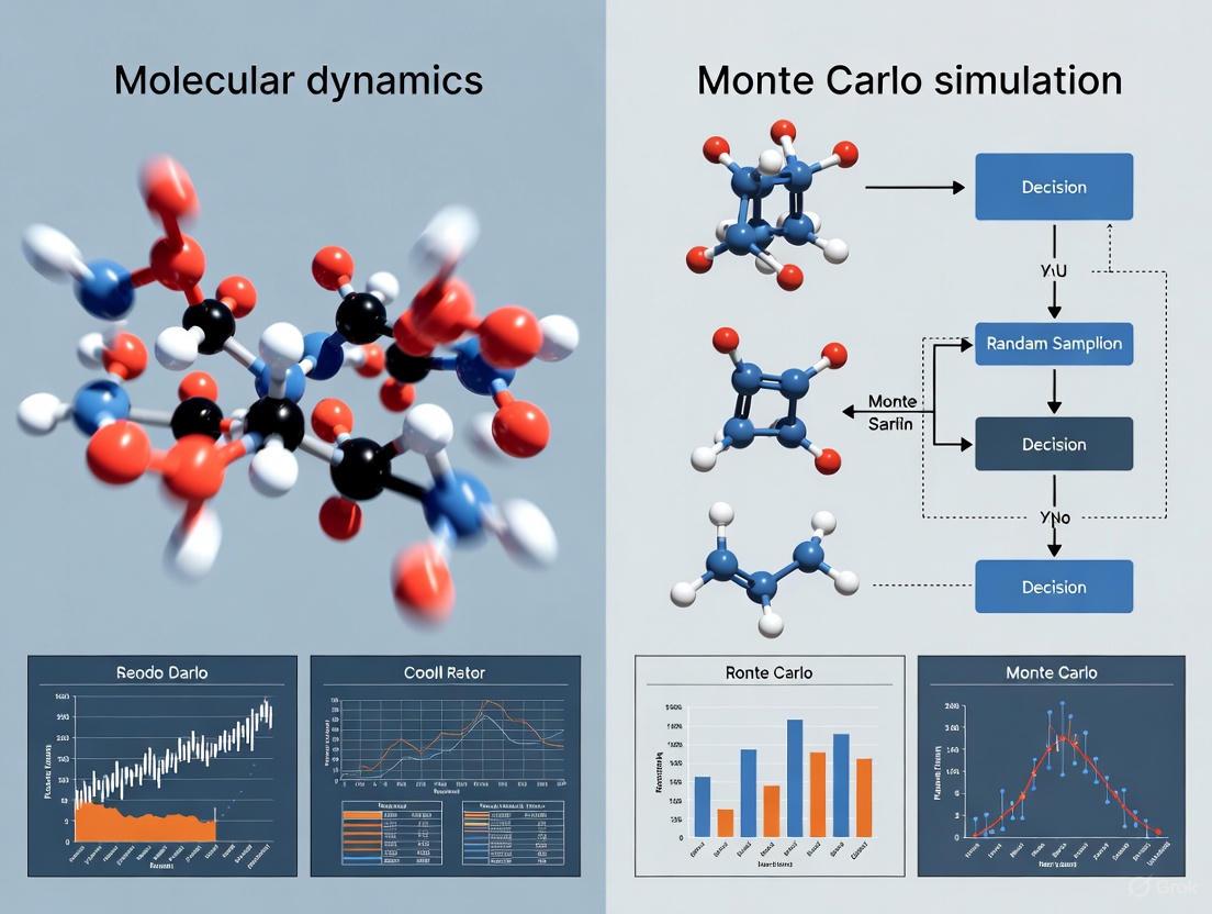
Workflow and Algorithmic Comparison
The following diagrams illustrate the fundamental workflows for Molecular Dynamics and Monte Carlo simulations, highlighting their deterministic versus probabilistic decision pathways.
Diagram 1: Molecular Dynamics Workflow
Diagram 2: Monte Carlo Workflow
Experimental Protocols and Validation
Case Study: Peptide Folding Simulations
A rigorous study applied both MD and MC principles to simulate eight helical peptides and validate against experimental circular dichroism measurements [5]. The protocol employed Replica Exchange Molecular Dynamics (REMD), which combines MD with a probabilistic temperature swapping approach.
Detailed REMD Protocol:
- Force Field: AMBER94 with generalized Born implicit solvent model [5]
- Temperature Ladder: 30 exponentially spaced temperatures from target (273-298K) to 624K [5]
- Simulation Time: Each replica ran for cycles of 1000 MD steps (2 ps) between swap attempts [5]
- Swap Criteria: Probabilistic exchange between adjacent temperatures based on Metropolis criterion [5]
- Convergence Monitoring: Statistical analysis of trajectory blocks to ensure adequate sampling [5]
This hybrid approach demonstrates how deterministic and probabilistic elements can be combined to enhance configurational sampling while maintaining physical dynamics in specific regions.
Case Study: High-Entropy Alloy Formation
A recent comparative study of a Cu-Fe-Ni-Mo-W multicomponent alloy directly contrasted pure MD and MC simulations with experimental results [6]. The research revealed significant differences in predictive accuracy:
Table 2: Comparison of MD and MC Predictions for Alloy Formation
| Method | Initial Structure | Predicted Phase Outcome | Agreement with Experiment |
|---|---|---|---|
| Molecular Dynamics | bcc | Single-phase bcc solid solution [6] | Poor |
| Molecular Dynamics | fcc | Single-phase fcc structure [6] | Poor |
| Monte Carlo | bcc | Two-phase mixture [6] | Moderate |
| Monte Carlo | fcc | bcc Fe-Mo-W phase + fcc Cu-Ni structure [6] | Strong |
Experimental validation through arc furnace production and powder milling confirmed a two-phase mixture of bcc and fcc structures, demonstrating MC's superior predictive power for this materials system [6]. The MC approach achieved lower potential energy states that more closely matched experimental observations.
Performance and Accuracy Comparison
Quantitative Assessment of Convergence and Sampling
The statistical nature of MC provides inherent advantages for certain types of equilibrium calculations, while MD excels at capturing dynamical behavior. The table below summarizes performance characteristics based on comparative studies:
Table 3: Performance Metrics for MD and MC Methods
| Metric | Molecular Dynamics | Monte Carlo |
|---|---|---|
| Equilibrium Sampling | Requires long simulations for ergodicity [5] | Efficient for Boltzmann sampling [2] |
| Parallelizability | Highly parallelizable (spatial decomposition) | Difficult to parallelize (sequential chain) [3] |
| Free Energy Calculation | Requires enhanced sampling techniques | Directly suited through ensemble generation [2] |
| Handling of Rare Events | May require specialized methods (metadynamics) | Natural handling through probabilistic jumps |
| Computational Cost | Costly for small timesteps (fs scale) [2] | Independent of timescales; configuration-based [2] |
| Accuracy for Dynamics | Provides realistic kinetics with proper force fields [5] | No natural time scale [2] |
Essential Research Reagent Solutions
Successful implementation of either MD or MC simulations requires specialized computational tools and force fields. The following table outlines essential "research reagents" for molecular simulations.
Table 4: Essential Research Reagents for Molecular Simulations
| Reagent / Tool Category | Specific Examples | Function & Purpose |
|---|---|---|
| Force Fields | AMBER, CHARMM, GROMOS, OPLS [5] | Define potential energy functions and parameters for molecular interactions |
| Solvation Models | Generalized Born, PME, Explicit Water Models [5] | Represent solvent effects and electrostatic interactions |
| Software Platforms | AMBER, GROMACS, LAMMPS, NAMD [5] | Provide simulation engines, integration algorithms, and analysis tools |
| Monte Carlo Engines | Cassandra, towhee, custom codes [2] | Specialized software for MC simulations with various ensemble capabilities |
| Enhanced Sampling Methods | Replica Exchange, Metadynamics, Umbrella Sampling [5] | Accelerate configuration space exploration and rare event sampling |
| Analysis Tools | MDAnalysis, VMD, PyMOL, custom scripts [5] | Process trajectories, calculate properties, and visualize results |
The choice between deterministic Molecular Dynamics and probabilistic Monte Carlo simulations must be guided by specific research questions and the nature of the properties under investigation. Molecular Dynamics is indispensable for studying time-dependent processes, transport phenomena, and dynamic behavior where temporal evolution is critical [2]. Conversely, Monte Carlo methods excel at calculating equilibrium properties, free energies, and sampling complex energy landscapes where physical dynamics would be prohibitively slow [4] [2].
Emerging hybrid approaches, such as Replica Exchange Molecular Dynamics [5] and specialized Monte Carlo techniques [6], demonstrate the power of combining deterministic and probabilistic elements to overcome the limitations of either method alone. As computational resources grow and algorithms advance, the integration of these complementary paradigms will continue to push the boundaries of predictive simulation in molecular science and drug development.
Molecular Dynamics (MD) and Monte Carlo (MC) are two foundational methods in computational physics and chemistry. While both are used to study molecular systems, their underlying principles and applications differ significantly. This guide provides a comparative analysis of these methods, focusing on the performance of specialized MD hardware and software against alternative simulation approaches.
Core Principles: Molecular Dynamics vs. Monte Carlo
The following table outlines the fundamental differences between Molecular Dynamics and Monte Carlo simulation methods.
Table 1: Fundamental Comparison of Molecular Dynamics and Monte Carlo Methods
| Feature | Molecular Dynamics (MD) | Monte Carlo (MC) |
|---|---|---|
| Theoretical Basis | Solves Newton's equations of motion to generate deterministic, time-evolving trajectories [7] [8]. | Uses random sampling based on the Metropolis criterion to generate probabilistic, energy-weighted configurations [9] [10]. |
| Primary Output | Time-series of atomic coordinates and velocities; reveals dynamical properties [8]. | Sequence of system states; provides structural and thermodynamic averages [6]. |
| Key Strengths | Calculates time-dependent properties (e.g., diffusion coefficients, mechanical properties) [8]. Efficiently explores complex free energy landscapes and is less constrained by system size [9] [6]. | |
| Inherent Limitations | Computationally expensive; limited by the femtosecond time-step, restricting access to long timescales [7] [9]. | Does not provide genuine dynamical information or kinetics [9]. |
| Typical Applications | Protein folding, drug binding kinetics, material deformation [7] [8]. | Protein folding thermodynamics, phase separation, multi-component alloy structure prediction [9] [6]. |
The core workflow of a Molecular Dynamics simulation involves iteratively calculating forces and integrating motion, as shown in the diagram below.
MD Simulation Cycle
Performance Comparison of Simulation Software
Specialized hardware like the MD-Engine was an early solution designed to accelerate the most computationally intensive part of MD: calculating non-bonding interactions, achieving good linear scaling with system size [11]. Today, this performance is largely delivered through GPU acceleration in software packages. The table below compares leading MD software tools.
Table 2: Performance and Features of Major Molecular Dynamics Software
| Software | Key Performance Features | Specialized Hardware/Acceleration | License |
|---|---|---|---|
| MD-Engine | Custom hardware accelerator; calculates pairwise potentials/forces in parallel; good linear scaling with system size [11]. | Dedicated, special-purpose MD processor [11]. | Proprietary Hardware |
| GROMACS | Extremely high throughput; multi-level parallelism; full GPU-resident workflows; among the highest single-GPU performance [12]. | GPU acceleration (CUDA/OpenCL); multi-node HPC scaling [12]. | Open Source (GPL/LGPL) |
| AMBER | Early and aggressive GPU optimization (PMEMD.CUDA); high throughput for single simulations on a single GPU [12]. | GPU acceleration; optimized for single-node, multi-GPU setups [12]. | AmberTools (Open Source), Full PMEMD (Paid) |
| NAMD | Fast, parallel MD; designed for parallel scalability across large CPU clusters; CUDA support [13]. | GPU acceleration; optimized for large-scale parallel CPU clusters [13]. | Free for Academic Use |
| CHARMM | Versatile MD engine with a rich set of features; effective parallel scaling on CPU clusters for moderate numbers of processors [12]. | Historically CPU-focused; less GPU-optimized than GROMACS/AMBER [12]. | Proprietary (Academic) |
| OpenMM | Highly flexible, scriptable via Python; high performance MD on GPUs [13]. | GPU acceleration; highly optimized for a wide range of GPUs [13]. | Open Source (MIT) |
| LAMMPS | Highly versatile for soft materials, solids, and coarse-grained systems; supports GPU acceleration [13]. | GPU acceleration; supports a wide range of interatomic potentials [13]. | Open Source (GPL) |
Experimental Protocols and Performance Data
Protocol for MD/MC Alloy Formation Study
A 2023 study directly compared MD and hybrid MD/MC for simulating a multi-component Cu-Fe-Ni-Mo-W high-entropy alloy [6].
- System Preparation: Initial structures were created as both Body-Centered Cubic (BCC) and Face-Centered Cubic (FCC) crystals.
- Simulation Parameters: Simulations were run from 10K up to the melting point of the alloy. The hybrid method combined MD's dynamical moves with MC's configurational sampling.
- Outcome Analysis: The resulting phases (BCC solid solution, FCC solid solution, or two-phase mixture) were analyzed and compared against experimentally produced samples using X-ray diffraction [6].
Performance Data: The study found that MD simulations starting from a BCC structure produced a single-phase BCC solid solution. In contrast, MC simulations produced a two-phase mixture, a result that was closer to the experimental findings, confirming MC's strength in predicting thermodynamic equilibrium structures [6].
Protocol for Enhanced Sampling MD with Machine Learning
To overcome the timescale limitation, MD is often combined with enhanced sampling and Machine Learning (ML) [7].
- Explorative MD: Run a preliminary, unbiased MD simulation to collect data on the system's fluctuations.
- ML Analysis: Apply ML algorithms (e.g., Dimensionality Reduction, Markov State Models) to the trajectory data to identify key collective variables (CVs) that describe the slowest, most important motions in the system [7].
- Informed Resampling: Use the identified CVs to perform biased sampling simulations (e.g., metadynamics), which selectively accelerate the exploration of these relevant pathways [7].
Performance Data: This MD/ML approach enhances sampling efficiency by focusing computational resources on the most relevant degrees of freedom, allowing for the calculation of free energy landscapes and the observation of rare events that would be inaccessible to standard MD [7].
Protocol for Large-Scale Cellular Monte Carlo
A 2025 study extended the MCell4 platform to simulate large-scale cellular dynamics, such as T cell immune synapse formation [10].
- Model Building: Create 3D meshes of cells (e.g., from microscopy or AI-generated models) and populate membranes with diffusing receptors and ligands.
- Force Integration: Introduce physical forces (kinetic, elastic, pressure) into the Monte Carlo framework, allowing molecular interactions to drive morphological changes.
- Simulation Execution: Run the Monte Carlo simulation, where steps are accepted or rejected based on a Metropolis criterion that considers the energy changes from both molecular interactions and membrane deformations [10].
Performance Data: This coupled MC approach successfully simulated the correlation between molecular interactions and the spreading dynamics of a T cell on an activating surface, demonstrating the ability of modern MC to handle complex, multi-scale biological feedback loops [10].
The Scientist's Toolkit: Essential Research Reagents and Materials
Table 3: Essential Software and Force Fields for Molecular Simulation
| Tool Name | Type | Primary Function |
|---|---|---|
| PLUMED [7] | Software Library | Enhances MD codes (e.g., GROMACS, AMBER) for enhanced sampling and free-energy calculations by biasing collective variables. |
| CHARMM-GUI [12] | Web Server | Simplifies the setup of complex simulation systems, such as membranes and protein-ligand complexes, for various MD engines. |
| Machine Learning Interatomic Potentials (MLIP) [8] | Force Field | Uses ML models trained on quantum chemistry data to perform highly accurate MD simulations at near-quantum accuracy and reduced cost. |
| Reactive Force Field (ReaxFF) [14] | Force Field | Enables MD simulations of chemical reactions by describing bond formation and breaking, bridging classical and quantum MD. |
| AlphaFold2 [8] | AI Model | Predicts 3D protein structures from amino acid sequences, providing reliable initial configurations for MD simulations. |
| VMD / PyMOL [13] [12] | Visualization Software | Used for visualizing simulation trajectories, analyzing molecular structures, and preparing figures for publication. |
The logical relationship between these tools in a modern simulation workflow is summarized below.
Modern Simulation Workflow
In computational science, particularly in fields like drug development, molecular dynamics (MD) and Monte Carlo (MC) simulations serve as indispensable tools for investigating molecular systems beyond the reach of experimental measurement [15]. While both methods aim to extract meaningful thermodynamic and structural properties from model systems, their fundamental sampling approaches differ significantly. At the core of many MC methods lies the Metropolis criterion, a decisive algorithm that enables efficient exploration of complex probability landscapes by strategically accepting or rejecting proposed moves [16]. This guiding principle allows MC methods to generate representative ensembles of molecular configurations without tracking system dynamics. In contrast, MD simulations numerically solve Newton's equations of motion to produce deterministic trajectories through phase space, capturing time-dependent phenomena but potentially facing challenges in crossing energy barriers. Understanding the performance characteristics, limitations, and complementary strengths of these approaches is crucial for researchers selecting appropriate methodologies for specific scientific challenges, from protein-ligand binding to materials design. This guide provides an objective comparison of these sampling engines, with particular emphasis on the role of the Metropolis criterion in MC methods and its impact on sampling efficiency in molecular simulation.
Core Algorithmic Foundations
The Metropolis-Hastings Algorithm
The Metropolis-Hastings algorithm is a Markov chain Monte Carlo (MCMC) method for obtaining a sequence of random samples from a probability distribution when direct sampling is difficult [16]. This algorithm operates through an iterative propose-and-decide process:
- Proposal Mechanism: From the current state ( xt ), a candidate state ( x' ) is generated from a proposal distribution ( g(x' \mid xt) ).
- Acceptance Probability: The candidate is accepted with probability ( \min(1, \alpha) ), where ( \alpha = \frac{P(x')}{P(x_t)} ) for symmetric proposal distributions [16].
- Markov Chain Construction: If accepted, ( x{t+1} = x' ); otherwise, ( x{t+1} = x_t ).
For Bayesian inference, where ( P(\theta \mid y) ) is the posterior distribution, the acceptance ratio simplifies to ( \frac{P(y \mid \theta2) P(\theta2)}{P(y \mid \theta1) P(\theta1)} ), eliminating the need to compute the typically intractable marginal likelihood [17]. This property makes the algorithm particularly valuable for practical Bayesian computation.
Molecular Dynamics Sampling
In contrast to MC's probabilistic state transitions, Molecular Dynamics employs numerical integration of Newton's equations of motion to simulate system evolution. The continuous equations ( F = ma ) are discretized using finite difference methods (e.g., Verlet algorithm), producing deterministic trajectories constrained to constant energy surfaces. To sample canonical ensembles, MD incorporates thermostats (e.g., Nosé-Hoover) that modify the equations of motion to maintain temperature, fundamentally altering the system dynamics [18]. This approach naturally captures time-dependent phenomena and transport properties but may suffer from slow convergence when energy landscapes contain high barriers that are rarely crossed during practical simulation timescales.
Performance Comparison: Quantitative Benchmarks
Sampling Efficiency in Coarse-Grained Polymer Systems
A comparative study of coarse-grained heteropolymers revealed significant methodological differences in sampling performance [18]. The researchers analyzed thermodynamic quantities and autocorrelation times using Andersen MD, Nosé-Hoover MD, and replica-exchange Monte Carlo methods, with the following key observations:
Table 1: Sampling Performance for Coarse-Grained Heteropolymers
| Method | Accuracy | Convergence Rate | Autocorrelation | Computational Cost per Step |
|---|---|---|---|---|
| Metropolis MC | High for equilibrium properties | Slow for rugged landscapes | High | Low |
| Replica-Exchange MC | Highest for multi-modal distributions | Fast due to barrier crossing | Reduced through exchange | High (multiple replicas) |
| Andersen MD | Moderate | Medium | Medium | Medium |
| Nosé-Hoover MD | Variable (serious quantitative differences found) | System-dependent | System-dependent | Medium |
The study found "serious quantitative differences" when using the Nosé-Hoover chain thermostat, highlighting how implementation details can significantly impact results [18]. MC methods demonstrated particular advantages for calculating equilibrium statistical properties where dynamical fidelity was unnecessary.
Reproducibility in Molecular Simulation
A comprehensive 2025 benchmarking study evaluated the replicability of MD and MC simulations for predicting alkane densities using the Molecular Simulation Design Framework (MoSDeF) [15]. The research involved multiple simulation engines performing identical simulation tasks:
Table 2: Density Prediction Performance Across Methods
| Method Type | Average Deviation from Experimental Density | Inter-method Variability | Statistical Uncertainty | Required Sampling Iterations |
|---|---|---|---|---|
| Monte Carlo (NpT) | Within 1% for most alkanes | Lower with standardized workflows | Small but consistently outside combined uncertainties | Varies by system; ~10^5-10^6 steps typically sufficient |
| Molecular Dynamics (NpT) | Within 1% for most alkanes | Higher due to implementation differences | Similar to MC | Dependent on integration time step; ~10^6-10^9 steps |
Notably, while most predicted densities were "reasonably close (mostly within 1%), the data often fell outside of the combined statistical uncertainties of the different simulations," indicating inherent methodological variations beyond random error [15]. The study concluded that "unavoidable errors inherent to molecular simulations" persist despite careful methodology, affecting both MD and MC approaches.
Experimental Protocols & Workflows
Standardized Benchmarking Methodology
To ensure fair comparison between MC and MD methods, the 2025 reproducibility study implemented rigorous standardized protocols [15]:
System Initialization: The MoSDeF toolkit initialized all system topologies, applied force fields consistently, and defined thermodynamic constraints uniformly across engines.
Ensemble Specification: Simulations were performed in the isothermal-isobaric (NpT) ensemble at identical state points for direct comparability.
Equilibration Criteria: Systems were equilibrated until properties (density, energy) stabilized with monitoring of running averages.
Production Sampling: Following equilibration, extended production runs generated statistical samples for analysis:
- MC: Minimum of 10^5 Monte Carlo steps after equilibration
- MD: Minimum of 10^6 integration steps with timesteps appropriate to the method (1-2 fs for atomistic)
Convergence Assessment: Block averaging techniques evaluated statistical uncertainties, with simulations extended until uncertainties fell below threshold values.
This workflow ensured that differences originated from methodological rather than implementation variability, providing a rigorous foundation for comparison.
Metropolis-Hastings Implementation Protocol
For the Metropolis-Hastings algorithm specifically, a standard implementation follows these steps [16] [17]:
Initialization: Start from an arbitrary point ( x_t ) in the parameter space.
Iteration Loop: For each iteration t:
- Proposal: Generate a candidate ( x' ) from the proposal distribution ( g(x' \mid x_t) ).
- Acceptance Ratio: Compute ( \alpha = f(x')/f(x_t) ) (ratio of target densities).
- Decision: Generate a uniform random number ( u \in [0,1] ):
- If ( u \leq \alpha ), accept candidate: ( x_{t+1} = x' )
- If ( u > \alpha ), reject candidate: ( x{t+1} = xt )
Termination: After a sufficient number of iterations (typically 10^3-10^6 depending on system complexity), the Markov chain's samples approximate the target distribution.
Hamiltonian Monte Carlo Protocol
As an advanced MC variant, Hamiltonian Monte Carlo (HMC) employs a physical approach to proposal generation [19]:
Momentum Sampling: Draw an initial momentum vector from a Gaussian distribution.
Hamiltonian Dynamics: Simulate trajectory evolution using discretized Hamiltonian equations:
- Number of steps (10-100) and step size adapted during warmup
- Uses gradient information for efficient high-dimensional sampling
Metropolis Acceptance: Apply standard Metropolis criterion to the proposed state at trajectory end.
No-U-Turn Extension: The No-U-Turn Sampler (NUTS) automatically determines optimal path lengths [19].
Key Software Solutions
Table 3: Essential Computational Tools for Molecular Simulation
| Tool Name | Type | Primary Function | Method Support |
|---|---|---|---|
| Stan | Probabilistic Programming | Bayesian inference using HMC and NUTS samplers | MC (HMC/NUTS) |
| MoSDeF | Workflow Framework | Standardized initialization of molecular simulations | Both MD and MC |
| signac | Workflow Management | Data management and workflow organization for simulation projects | Both MD and MC |
| REMC | Algorithm | Replica-exchange for enhanced sampling in multi-modal distributions | MC |
| Nosé-Hoover | Thermostat | Temperature control for constant-temperature MD simulations | MD |
Critical Algorithmic Components
Metropolis Criterion: The decision rule that accepts or rejects proposed state transitions with probability ( \min(1, \alpha) ), ensuring detailed balance and correct sampling of the target distribution [16].
Proposal Distribution: The function ( g(x' \mid x) ) that suggests new candidate states, significantly impacting sampling efficiency through optimal step size selection [16].
Force Field: The mathematical model describing interatomic interactions (e.g., Lennard-Jones potentials, bonded terms), common to both MD and MC simulations [15].
Thermodynamic Ensemble: The statistical mechanical constraints (NpT, NVT, etc.) applied to the system, with MC naturally accommodating various ensembles through modified acceptance criteria [15].
Comparative Analysis: Strategic Selection Guidelines
Method Selection Criteria
Choosing between MC and MD approaches requires careful consideration of research objectives:
Prefer MC Methods When:
- Sampling equilibrium distributions without dynamical information
- Working with complex boundary conditions or variable particle numbers
- System has high energy barriers that benefit from specialized moves
- Implementing enhanced sampling techniques like replica-exchange
Prefer MD Methods When:
- Studying time-dependent phenomena and transport properties
- Investigating kinetics and pathway mechanisms
- System requires natural dynamics without artificial moves
- Analyzing correlation functions and spectral properties
Emerging Trends and Future Directions
The convergence of MD and MC methodologies represents a significant trend in molecular simulation. Modern implementations increasingly incorporate strengths from both approaches:
- Hybrid Methods: Combining MD's local exploration with MC's barrier-crossing capabilities
- Enhanced Sampling: Techniques like metadynamics and parallel tempering borrowing concepts from both traditions
- Machine Learning Integration: Neural networks guiding proposal generation in MC and force evaluation in MD
- Workflow Standardization: Frameworks like MoSDeF enabling direct comparison and method validation [15]
The 2025 MCM conference will highlight cutting-edge developments in these areas, particularly advancements in Hamiltonian Monte Carlo and non-equilibrium candidate Monte Carlo methods [20].
The Metropolis criterion continues to serve as the fundamental engine driving Monte Carlo sampling methods, providing a mathematically rigorous foundation for exploring complex molecular systems. While Molecular Dynamics offers unique capabilities for investigating temporal evolution and dynamic processes, MC methods maintain distinct advantages for equilibrium sampling, particularly when enhanced with modern algorithms like Hamiltonian Monte Carlo. The demonstrated 1% accuracy in density prediction for both approaches [15] confirms their reliability for many drug discovery applications, from hERG channel liability assessment [21] to protein classification. As the field progresses toward standardized workflows and TRUE (Transparent, Reproducible, Usable-by-others, Extensible) principles [15], researchers can select between these complementary approaches with greater confidence, leveraging their respective strengths to address the complex challenges of modern molecular design and drug development.
Molecular Dynamics (MD) and Monte Carlo (MC) simulations are foundational techniques in computational physics and chemistry. While they share the goal of sampling molecular configurations, their core principles and primary outputs differ significantly. MD simulations generate realistic temporal dynamics by numerically solving Newton's equations of motion, providing insights into time-dependent processes. In contrast, MC simulations utilize random sampling to generate thermodynamic ensembles, excelling at calculating equilibrium properties and free energies. This guide provides an objective comparison of these methods, supported by current research and experimental data, to help researchers select the appropriate tool for their scientific objectives.
Methodological Comparison: Core Principles and Outputs
The fundamental difference between MD and MC lies in their sampling approach and the type of information they yield. The table below summarizes their key characteristics.
Table 1: Fundamental Comparison of MD and MC Simulation Methods
| Feature | Molecular Dynamics (MD) | Monte Carlo (MC) |
|---|---|---|
| Sampling Basis | Numerical integration of equations of motion; deterministic time evolution [22]. | Stochastic random moves based on acceptance criteria; sequence of states without time correlation [9]. |
| Primary Output | Trajectories in phase space; temporal evolution and dynamic properties [22]. | Thermodynamic ensembles (e.g., NVT, NPT); equilibrium averages and free energies [9]. |
| Key Strength | Calculation of time-dependent properties (e.g., diffusion coefficients, viscosity) [23]. | Efficient sampling of complex energy landscapes and calculation of equilibrium properties [9]. |
| Inherent Limitation | Computationally expensive; can struggle to sample rare events or complex landscapes [22]. | Does not provide genuine kinetic information or time scales [9]. |
| Typical Application | Studying transport properties, protein folding pathways, and finite-temperature dynamics [24] [23]. | Determining stable molecular crystal forms, protein folding equilibria, and phase transitions [25] [9]. |
Quantitative Performance Data from Recent Studies
Recent applications highlight the complementary strengths of MD and MC in predicting different classes of properties. Performance is highly dependent on the specific scientific question and the quality of the underlying force field or potential.
Table 2: Comparison of Key Outputs from Recent MD and MC Studies
| System Studied | Methodology | Key Predicted Outputs | Agreement with Experiment | Citation |
|---|---|---|---|---|
| Water (across a broad temperature range) | MD with a machine-learned potential (NEP-MB-pol) | Dynamic Properties: Self-diffusion coefficient, viscosity, thermal conductivity.Thermodynamic Properties: Density, heat capacity.Structural Properties: Radial distribution function. | Quantitative agreement for all three transport coefficients and structural properties [23]. | [23] |
| Molecular Crystals (X23 dataset) | MC and MD simulations with Machine Learning Interatomic Potentials (MLIPs) | Thermodynamic Properties: Sublimation enthalpies, lattice energies, finite-temperature stability [25]. | Sub-chemical accuracy (< 4 kJ mol⁻¹) for sublimation enthalpies [25]. | [25] |
| Bounded One-Component Plasma (BOCP) | MD with explicit boundary conditions | Thermodynamic Properties: Total electrostatic energy, ionic compressibility factor, ionic equation of state [26]. | Estimated relative error ~0.1% for electrostatic energy; provides reference data for other methods [26]. | [26] |
| Intrinsically Disordered Proteins (IDPs) | MD (GaMD) for conformational sampling | Dynamic/Temporal Output: Conformational ensembles, proline isomerization events, identification of transient states [22]. | Generated ensembles aligned with experimental circular dichroism data [22]. | [22] |
| Protein-Ligand Binding | MD simulations in explicit solvent | Thermodynamic Output: Change in heat capacity (ΔCp) upon ligand binding [27]. | Predictions were similar to experimental values and could discriminate effective inhibitors [27]. | [27] |
Experimental Protocols and Workflows
Protocol for MD Simulation of Ion Transport in Solids
A compact guide for performing reliable MD simulations of ion transport in solids outlines a critical workflow [28]:
- System Preparation: Carefully construct the simulation cell, avoiding common pitfalls that lead to incorrect results.
- Equilibration: Systematically examine and determine the optimal equilibration time for the system.
- Production Simulation: Execute the MD run, confirming the transition from subdiffusive to diffusive behavior of ions.
- Data Analysis: Evaluate diffusion data as a function of temperature. Extrapolate data and interpret results in the context of experimental findings [28].
Protocol for Monte Carlo in Biomolecular Systems
A workshop on atomistic MC simulations for biomolecular systems details its application [9]:
- System Setup: Parametrize the model, often using a physics-based force field for full transferability.
- Sampling: Perform Markov-chain Monte Carlo sampling to generate states. This often involves:
- Unbiased Folding Simulations: To explore the free energy landscape of processes like protein folding.
- Combination with MD: Using MC to circumvent time-scale barriers typical for MD alone.
- Analysis: Generate and analyze free energy landscapes. The primary outputs are equilibrium ensembles and thermodynamic properties, not time-series data [9].
Workflow for Predicting Protein-Ligand Binding Thermodynamics via MD
A study on predicting heat capacity changes (ΔCp) upon ligand binding uses the following MD protocol [27]:
- System Preparation: Create four systems in a water sphere: the protein, the free ligand, the protein-ligand complex, and pure water. The number of water molecules must be identical in all spheres.
- Calibration: Perform separate MD simulations of pure water under identical conditions to calibrate the solvent's contribution to the heat capacity.
- Simulation Series: Run MD simulations for the protein, ligand, and complex across a range of temperatures (e.g., 280 K to 320 K).
- Energy Calculation: For each temperature, calculate the average total energy
<U>for each system. - Heat Capacity Calculation: Subtract the calibrated water contribution from the total heat capacity of each system. The change in heat capacity upon binding,
ΔCp, is then calculated using the formula:ΔCp = [∂<U>/∂<T>]_complex - [∂<U>/∂<T>]_protein - [∂<U>/∂<T>]_ligand[27].
The Scientist's Toolkit: Essential Research Reagents and Solutions
Modern simulations, both MD and MC, rely on a suite of software and models to achieve accuracy and efficiency.
Table 3: Essential Research Reagents and Computational Tools
| Tool / Solution | Type | Primary Function | Citation |
|---|---|---|---|
| Machine Learning Interatomic Potentials (MLIPs) | Model / Potential | Bridges the accuracy of quantum mechanics and the speed of classical force fields for MD and MC energy calculations [25] [23]. | [25] [23] |
| MACE-MP-0 | Foundation ML Model | A pre-trained MLIP that can be fine-tuned with minimal data (~200 structures) for accurate simulations of molecular crystals [25]. | [25] |
| Neuroevolution Potential (NEP) | Machine-Learned Potential | A framework for generating highly efficient MLPs; used for accurate modeling of water's thermodynamic and transport properties via MD [23]. | [23] |
| OMol25 Dataset | Training Data | A massive dataset of high-accuracy quantum chemical calculations used to train neural network potentials for improved molecular modeling [29]. | [29] |
| Path-Integral Molecular Dynamics (PIMD) | Simulation Method | An MD technique that accounts for nuclear quantum effects, crucial for accurately predicting properties like heat capacity and diffusion [23]. | [23] |
| ProFASi Software | Simulation Software | A software package for performing Monte Carlo simulations of proteins, enabling tasks like unbiased protein folding [9]. | [9] |
| LAMMPS | Simulation Engine | A widely used molecular dynamics simulator that can be adapted for specialized simulations like one-component plasma [26]. | [26] |
MD and MC are not competing methods but rather complementary tools in the computational scientist's arsenal. The choice between them is dictated by the research question. MD is indispensable for investigating kinetics, transport coefficients, and any process where the time-evolution and dynamical nature of the system are paramount. MC is superior for efficiently sampling complex equilibrium ensembles, calculating absolute free energies, and determining the relative stability of states, particularly when realistic dynamics are not required. The integration of machine-learning potentials is enhancing the accuracy and scope of both techniques, pushing the boundaries of what is possible in computational molecular science.
Molecular Dynamics (MD) and Monte Carlo (MC) simulations are foundational techniques in computational materials science and drug development. Despite their methodological differences, both approaches rely on the accurate description of interatomic interactions through force fields and the calculation of system energies to predict material behavior and molecular properties. This guide provides a detailed comparison of their performance, supported by experimental data and protocols.
Force Fields: The Common Computational Backbone
Force fields are mathematical expressions that describe the potential energy of a system as a function of the nuclear coordinates. Both MD and MC simulations utilize these force fields to model interactions, making their accuracy paramount. A typical force field includes terms for bonded interactions (bonds, angles, dihedrals) and non-bonded interactions (van der Waals, electrostatic).
Table 1: Common Force Field Terms and Their Mathematical Expressions
| Energy Component | Mathematical Expression | Description |
|---|---|---|
| Bond Stretching | $E{bond} = \sum{bonds} kb(r - r0)^2$ | Harmonic potential for covalent bond vibration. |
| Angle Bending | $E{angle} = \sum{angles} k{\theta}(\theta - \theta0)^2$ | Harmonic potential for angle vibration. |
| Torsional Dihedral | $E{dihedral} = \sum{dihedrals} \frac{V_n}{2}[1 + \cos(n\phi - \gamma)]$ | Periodic potential for bond rotation. |
| van der Waals | $E{vdW} = \sum{i |
Lennard-Jones potential for dispersion/repulsion. |
| Electrostatic | $E{elec} = \sum{i |
Coulomb's law for interactions between partial charges. |
The parameterization of these force fields is critical. For example, in hydration free energy (HFE) calculations, the OPLS-AA force field combined with the TIP4P water model has been a standard, though it systematically overestimates the hydrophobicity of hydrocarbons. Recent work shows that scaling the Lennard-Jones interactions between water oxygen and carbon atoms by a factor of 1.25 can reduce the mean unsigned error in HFE predictions from 1.0-1.2 kcal/mol to 0.4 kcal/mol [30]. Furthermore, Machine Learning Force Fields (MLFFs) are emerging as a promising avenue to retain quantum mechanical accuracy at a reduced computational cost, as demonstrated by the Organic_MPNICE model achieving sub-kcal/mol errors on a diverse set of organic molecules [31].
Methodological Comparison: Divergence in Application
While MD and MC share a foundation in force fields, their core algorithms and the properties they can efficiently probe differ significantly. The choice between them depends on the specific scientific question.
Core Algorithmic Principles
Molecular Dynamics (MD) is a deterministic method that numerically integrates Newton's equations of motion. It generates a time-evolving trajectory of the system, providing direct insight into dynamical properties such as diffusion coefficients, viscosity, and time-dependent responses [3]. Its strength lies in capturing realistic system dynamics but is limited to relatively short timescales (typically nanoseconds to microseconds).
Monte Carlo (MC) is a probabilistic method that generates a series of random states, accepting or rejecting them based on a probabilistic criterion (e.g., the Metropolis criterion). It excels at sampling configuration space to efficiently compute equilibrium properties and free energies but contains no inherent concept of time [30] [3]. This makes it unsuitable for studying kinetic or transport properties directly.
Performance in Free Energy Calculations
Free energy is a key thermodynamic property critical for predicting binding affinities in drug discovery and solubility in materials science. MC simulations, particularly with Free Energy Perturbation (FEP) theory, have a long history of providing highly accurate results for these properties [30].
Table 2: Comparison of HFE Calculation Performance (OPLS-AA Force Field)
| Method / Model | System / Test Case | Mean Unsigned Error (kcal/mol) | Key Finding |
|---|---|---|---|
| MC/FEP (Standard) | 50 organic molecules | 1.0 - 1.2 | Systematic overestimation of hydrophobicity. |
| MC/FEP (Scaled LJ) | 50 organic molecules | 0.4 | Scaling LJ interactions improves accuracy [30]. |
| MLFF (Organic_MPNICE) | 59 organic molecules | < 1.0 | Achieves ab initio quality without parameter tuning [31]. |
| Classical MD/FEP | Varies | Typically > 1.0 | Accuracy limited by force field, not MD methodology. |
Experimental Protocol for MC/FEP HFE Calculation:
- System Setup: A single solute molecule is placed in a periodic cubic box containing 500 TIP4P water molecules for the solution phase, and in vacuum for the gas phase [30].
- Sampling: MC simulations are performed in the isothermal-isobaric (NPT) ensemble at 25°C and 1 atm. The solute's internal degrees of freedom are sampled using a Z-matrix.
- Annihilation: The solute is "annihilated" (its interactions are turned off) in both the gas and solution phases using FEP. This involves running a series of 20+ "windows" where a coupling parameter (λ) gradually scales the solute's Coulomb and Lennard-Jones interactions to zero.
- Free Energy Calculation: The free energy change for annihilation in both phases is computed from the simulations. The difference between these values yields the absolute hydration free energy: ΔGhyd = ΔGsolv - ΔGgas [30].
Simulating Complex Materials: High-Entropy Alloys
The performance of MD and MC can diverge significantly when modeling complex, multi-component systems. A study on a Cu-Fe-Ni-Mo-W high-entropy alloy highlights this difference.
Experimental Protocol for Alloy Phase Formation [6]:
- Model Construction: Initial structures were created as either body-centered cubic (bcc) or face-centered cubic (fcc) lattices.
- Simulation Execution: Hybrid MD/MC simulations were performed, heating the models from 10K up to their melting points.
- Analysis: The final phase composition and potential energy of the systems were analyzed and compared to experimentally produced alloys (via arc melting and powder milling).
Results: MD simulations starting from a bcc structure predicted a single-phase bcc solid solution. In contrast, MC simulations produced a two-phase mixture of a bcc Fe-Mo-W phase and a fcc Cu-Ni phase. This MC result aligned closely with the experimental data, which also showed a two-phase mixture, demonstrating MC's superior capability in predicting equilibrium phase separation in this complex system [6].
Hybrid Methods: Bridging the Timescale Gap
A major limitation of standard MD is its inability to access the long timescales required for slow processes like solid-state diffusion. Kinetic Monte Carlo (kMC) can address this but often relies on simplified, rigid-lattice models. A powerful solution is to combine the strengths of both methods in a hybrid approach.
Workflow of a Hybrid MD/kMC Algorithm for Accelerated Diffusion [32]:
- KMC Step Initiation: A random atom is selected within an MD simulation.
- Neighbor Identification: All first-nearest-neighbor atoms of the selected atom are identified.
- Swap Attempt and Acceptance: A swap between the selected atom and one of its neighbors is attempted. The move is accepted or rejected based on the energy change and the kMC acceptance probability.
- MD Simulation Continuation: The standard MD simulation continues from the new atomic configuration. This process artificially accelerates diffusion to a rate observable on MD timescales [32].
This MD/kMC hybrid, implemented in LAMMPS, allows researchers to study diffusion-dependent phenomena like precipitate growth and solute drag effects without needing a priori knowledge of all possible atomic transition states, a requirement for traditional kMC [32].
The Scientist's Toolkit: Essential Research Reagents
Table 3: Key Software and Force Fields for Molecular Simulation
| Tool Name | Type | Primary Function | Key Application |
|---|---|---|---|
| LAMMPS | Software | A highly versatile and widely-used MD simulator. | Large-scale atomic/molecular modeling; supports hybrid MD/kMC [32]. |
| BOSS | Software | A general modeling program for MC simulations. | Specialized for free energy calculations (FEP) in organic and biochemical systems [30]. |
| OPLS-AA | Force Field | An all-atom force field for organic molecules. | Predicting properties of liquids and free energies of hydration [30]. |
| TIP4P | Water Model | A 4-site rigid water model. | The solvent model of choice for many accurate MC/FEP hydration studies [30]. |
| Organic_MPNICE | Machine Learning FF | A broadly trained ML force field. | Achieving quantum-mechanical accuracy in HFE predictions for diverse molecules [31]. |
In Practice: Methodological Workflows and Drug Discovery Applications
Molecular Dynamics (MD) represents a cornerstone technique in computational molecular sciences for studying system evolution over time. Unlike its probabilistic counterpart, Monte Carlo (MC), which excels at sampling equilibrium configurations but cannot model time-dependent processes, MD is a deterministic method that solves equations of motion to simulate dynamical trajectories [3]. This fundamental difference dictates their respective applications: MD is indispensable for investigating kinetic properties, transport phenomena, and non-equilibrium processes, while MC often proves more efficient for determining equilibrium states and thermodynamic properties in systems where dynamics are not the primary concern [3]. The choice between them hinges on whether the scientific question requires temporal resolution or focuses solely on equilibrium sampling. Within this broader context of computational sampling methodologies, this guide details the established workflow for MD simulations, from initial system preparation through to trajectory analysis, highlighting how this approach complements MC techniques in the researcher's toolkit.
The Core Molecular Dynamics Workflow
A robust MD workflow consists of several interconnected stages, each critical for ensuring the physical relevance and statistical reliability of the simulation results. The entire process is iterative, with analysis often informing refinements to the system setup or simulation parameters.
Figure 1: The core, iterative stages of a Molecular Dynamics (MD) simulation workflow.
System Setup
The initial phase involves constructing the molecular system and defining the computational environment. For a protein-ligand complex in drug discovery, this entails obtaining the 3D structure from a database like the Protein Data Bank (PDB), parameterizing the ligand using tools like antechamber (if using AMBER) or CGenFF (if using CHARMM), and embedding the system in a solvent box (e.g., TIP3P water model) with added ions to neutralize the system's charge and achieve physiological ionic strength [33]. The choice of force field (e.g., CHARMM, AMBER, GROMOS) is critical, as it defines the potential energy function and associated parameters governing atomic interactions [33] [34]. For materials science applications, such as simulating Calcium Aluminosilicate Hydrate (CASH), the initial configuration might be built from a crystalline template like tobermorite, followed by atomic substitutions and hydration to model the amorphous gel structure [34].
Energy Minimization and Equilibration
Before dynamics can begin, the system must be relaxed to remove unfavorable atomic clashes and high-energy strains introduced during setup. Energy minimization employs algorithms like steepest descent or conjugate gradient to find the nearest local energy minimum. Subsequently, equilibration is performed to bring the system to the desired thermodynamic state (e.g., NVT and NPT ensembles). During NVT equilibration, the system's temperature is gradually increased and stabilized using thermostats (e.g., Nosé-Hoover, Berendsen), while NPT equilibration adjusts the system's density using barostats (e.g., Parrinello-Rahman) to reach the target pressure [34]. This phase ensures the system is stable and representative of the experimental conditions before data collection begins.
Production Run and Trajectory Analysis
The production phase involves integrating Newton's equations of motion over a defined period (nanoseconds to microseconds) to generate the trajectory—a file containing the atomic coordinates and velocities over time. The length of this simulation is determined by the biological or physical process of interest. Analysis of this trajectory extracts scientifically meaningful information. Key properties include the Root Mean Square Deviation (RMSD), which measures structural stability; the Root Mean Square Fluctuation (RMSF), which identifies flexible regions; the Radius of Gyration, which assesses compactness; and the Solvent Accessible Surface Area (SASA), which quantifies surface exposure [35] [33]. For solvation studies, properties like the Average number of solvents in the Solvation Shell (AvgShell) and Estimated Solvation Free Energies (DGSolv) are critical [35].
Comparative Analysis: MD vs. Monte Carlo Performance
The choice between MD and MC is not merely philosophical but has practical implications for computational cost, accuracy, and the type of information that can be obtained. The table below summarizes key differentiators based on recent research.
Table 1: Comparative analysis of Molecular Dynamics and Monte Carlo simulation methods.
| Feature | Molecular Dynamics (MD) | Monte Carlo (MC) |
|---|---|---|
| Fundamental Principle | Deterministic; integrates Newton's equations of motion [3] | Probabilistic; accepts/rejects configurations based on Boltzmann probability [3] |
| Native Simulation Ensemble | Microcanonical (NVE), but others can be simulated [3] | Canonical (NVT), Isothermal-isobaric (NPT) [3] |
| Temporal Resolution | Provides realistic time evolution and dynamics [3] | No real-time dynamics; only samples equilibrium states [3] |
| Handling of Complex Potentials | Formally more exact but can suffer from slow convergence [36] | Efficient for on-lattice models; challenging for fully flexible molecules [3] |
| Parallelization | Highly parallelizable (e.g., in GPUs) [3] | Difficult to parallelize due to sequential acceptance/rejection steps [3] |
| Applicability to Non-Equilibrium | Suitable for both equilibrium and non-equilibrium systems [3] | Primarily suited for equilibrium sampling [3] |
| Performance in Alloy Formation | Predicted incorrect single-phase BCC solid solution [6] | Correctly predicted two-phase mixture, matching experiments [6] |
| Computational Demand for Folding | Very expensive for all-atom protein folding simulations [3] | Can be more efficient for conformational sampling at equilibrium [3] |
Experimental data from a 2023 study on a Cu–Fe–Ni–Mo–W high-entropy alloy provides a concrete performance comparison. The MD simulation, starting from a body-centered cubic (BCC) structure, incorrectly predicted the formation of a single-phase BCC solid solution. In contrast, the MC simulation accurately produced a two-phase mixture, a result later confirmed by experimental production using arc furnace and powder milling [6]. This demonstrates MC's potential superiority in predicting certain equilibrium phase distributions.
In polymer science, a 2021 study compared MD, Self-Consistent Field (SCF) theory, and a hybrid Monte Carlo SCF (MC-SCF) method for modeling polymer stars. The MD approach was noted as "formally the most exact" but was hampered by "reasonable convergence" issues. The hybrid MC-SCF method successfully combined the benefits of accurate sampling with computational efficiency, performing well across a range of solvent conditions [36].
Experimental Protocols and Data Analysis
Detailed Protocol: Drug Solubility Prediction via MD
A 2025 study on predicting drug aqueous solubility (logS) offers a detailed MD protocol suitable for biomolecular applications [35].
Methodology:
- System Preparation: A dataset of 211 drugs was compiled. Each drug molecule was placed in a cubic simulation box (e.g., 4 nm side length) solvated with water molecules.
- Force Field and Software: Simulations were conducted using GROMACS 5.1.1 with the GROMOS 54a7 force field [35].
- Simulation Parameters: Simulations were run in the NPT ensemble (constant Number of particles, Pressure, and Temperature) to mimic experimental conditions.
- Production Run: A production MD run was performed to generate a stable trajectory for analysis.
- Property Extraction: Ten MD-derived properties were extracted from the trajectory for each drug, including SASA, Coulombic and Lennard-Jones (LJ) interaction energies, DGSolv, RMSD, and AvgShell. The octanol-water partition coefficient (logP) was also included from experimental literature.
- Machine Learning Modeling: These properties were used as features to train ensemble machine learning models (e.g., Gradient Boosting) to predict experimental logS.
Results and Analysis: The study found that a subset of seven properties—logP, SASA, Coulombic_t, LJ, DGSolv, RMSD, and AvgShell—were highly effective predictors of solubility. The Gradient Boosting model achieved a predictive R² of 0.87 and an RMSE of 0.537 on the test set, demonstrating that MD-derived properties have predictive power comparable to models based solely on structural fingerprints [35].
Table 2: Key MD-derived properties used for predicting drug aqueous solubility with machine learning [35].
| Property | Description | Role in Solubility |
|---|---|---|
| logP | Octanol-water partition coefficient (experimental) | Measures hydrophobicity/hydrophilicity |
| SASA | Solvent Accessible Surface Area | Quantifies surface exposed to solvent |
| Coulombic_t | Coulombic interaction energy with solvent | Measures polar interactions with water |
| LJ | Lennard-Jones interaction energy with solvent | Measures van der Waals interactions |
| DGSolv | Estimated Solvation Free Energy | Overall energy change upon solvation |
| RMSD | Root Mean Square Deviation | Indicates conformational stability |
| AvgShell | Avg. number of solvents in Solvation Shell | Describes the local solvation environment |
Workflow Automation with AI Agents
Recent advances have introduced automation to the complex MD workflow. The MDCrow framework, an LLM (Large Language Model) agent, exemplifies this trend. It uses over 40 expert-designed tools for tasks like retrieving PDB files, cleaning structures with PDBFixer, setting up simulations in OpenMM, adding solvent with PackMol, and performing analysis with MDTraj for properties like RMSD and radius of gyration [33]. This automation reduces the expert intuition traditionally required for parameter selection and multi-step preprocessing and analysis, making MD more accessible and reproducible.
The Scientist's Toolkit
Table 3: Essential software and tools for a modern Molecular Dynamics workflow.
| Tool Name | Type | Primary Function |
|---|---|---|
| GROMACS | Simulation Software | High-performance MD package for simulating Newtonian dynamics [35] |
| AMBER | Simulation Software | Suite of programs for simulating biomolecules [33] |
| CHARMM | Simulation Software | Versatile MD simulation program with extensive force fields [33] |
| OpenMM | Simulation Software | Toolkit for MD simulation with high GPU performance [33] |
| MDTraj | Analysis Library | Software library for analyzing MD simulations [33] |
| PDBFixer | Utility Tool | Corrects common problems in PDB files (e.g., missing residues) [33] |
| PackMol | Utility Tool | Prepulates initial configurations by packing molecules in a simulation box [33] |
| MDCrow | Workflow Automation | LLM agent for automating setup, simulation, and analysis tasks [33] |
| Simple Active Learning | Advanced Workflow | Workflow for on-the-fly training of machine learning potentials during MD [37] |
A typical MD workflow is a structured process encompassing system setup, energy minimization, equilibration, production simulation, and trajectory analysis. While MD is a powerful and deterministic tool for studying time-dependent phenomena, its position in research is defined in contrast to the Monte Carlo method. MC, as a probabilistic sampler, often proves more efficient and sometimes more accurate for predicting equilibrium properties, as evidenced by its success in modeling alloy phase behavior [6]. The choice between them should be guided by the research question: MD for dynamics and kinetics, MC for equilibrium thermodynamics. Future directions point toward greater automation through AI agents [33] and the integration of machine learning potentials to enhance accuracy and speed [37], further solidifying the role of MD as an indispensable tool in computational science.
Molecular Dynamics (MD) and Monte Carlo (MC) simulations represent two foundational pillars in computational molecular science. While both aim to sample molecular configurations to compute thermodynamic properties, their fundamental approaches differ significantly. MD simulations generate ensembles by numerically solving Newton's equations of motion, providing a time-evolving trajectory of the system. In contrast, MC methods utilize random sampling to generate configurations according to appropriate statistical mechanical distributions, typically calculating thermodynamic properties via an ensemble average rather than a time average.
For ergodic systems, these approaches converge to identical results, yet each offers distinct advantages and limitations that make them suitable for different research scenarios. This guide provides a comprehensive comparison of these methodologies, focusing specifically on elucidating the typical MC workflow for configuration generation and observables calculation, while contextualizing its performance relative to MD approaches.
The Core MC Workflow: From Configurations to Observables
A typical Monte Carlo simulation follows a structured workflow to generate statistically independent molecular configurations and compute observable properties from them. The process involves careful preparation, iterative configuration generation, and rigorous statistical analysis, with particular attention to quantifying uncertainty.
The following diagram illustrates the standard MC workflow, highlighting the cyclical nature of configuration generation and the critical steps for calculating observables with proper uncertainty quantification:
Configuration Generation Methodology
Configuration generation in MC relies on Markov chain Monte Carlo methods, where new configurations are generated through random perturbations of the current state. The core algorithm follows these steps:
Initialization: The simulation begins with an initial configuration, which could be a crystal lattice, random arrangement, or pre-equilibrated structure. The choice of statistical ensemble (NVT, NPT, etc.) determines which thermodynamic variables remain fixed.
Random Move Proposal: The algorithm proposes a random modification to the current configuration. Common moves include:
- Translating a randomly selected particle
- Rotating a molecule or molecular fragment
- Changing molecular conformation (e.g., dihedral angle rotation)
- Modifying simulation box dimensions (in NPT ensemble)
- Cluster moves or swap moves for complex systems
Energy Evaluation: After each move, the potential energy change (ΔE) between the new and old configurations is computed using the chosen force field or potential energy function.
Metropolis Criterion: The move is accepted or rejected based on the Metropolis acceptance criterion, which depends on the Boltzmann factor of the energy change:
- If ΔE ≤ 0, the move is always accepted
- If ΔE > 0, the move is accepted with probability exp(-ΔE/kBT) This ensures detailed balance and generates configurations according to the Boltzmann distribution.
Observables Calculation and Uncertainty Quantification
Once configurations are generated, observables are calculated as ensemble averages over the sampled states. For a general observable O, the ensemble average is computed as:
⟨O⟩ = (1/N) Σ O(config_i)
where the sum runs over N statistically independent configurations.
A critical aspect often overlooked in MC simulations is proper uncertainty quantification (UQ). Statistical uncertainties must be reported alongside any simulated observable to communicate the significance and limitations of the results [38]. Key statistical concepts include:
- Arithmetic mean: The estimate of the true expectation value of a random quantity
- Experimental standard deviation: An estimate of the true standard deviation of a random variable
- Standard uncertainty: Uncertainty in a result expressed in terms of a standard deviation
- Experimental standard deviation of the mean: An estimate of the standard deviation of the distribution of the arithmetic mean (often called "standard error") [38]
For correlated data, special care must be taken. The correlation time (τ) is the longest separation in "time" (simulation steps) for which configurations remain correlated. For observables computed from correlated data, the effective sample size is reduced to N/τ, which increases the statistical uncertainty [38].
In specialized MC variants like Diagrammatic Quantum Monte Carlo, where configurations can have complex weights w(c) = φ_c|w(c)|, observables are calculated using a modified approach:
⟨O⟩ = ⟨Oφc⟩{|w(c)|} / ⟨φc⟩{|w(c)|}
where the averages on the right-hand side are taken with respect to the absolute value of the weights. In such cases, the average complex sign ⟨φ_c⟩ must be real, and the real parts of both numerator and denominator are typically used to obtain real-valued observables [39].
Comparative Analysis: MC vs. MD Performance
Methodological Comparison
Table 1: Fundamental methodological differences between MC and MD approaches
| Aspect | Monte Carlo (MC) | Molecular Dynamics (MD) |
|---|---|---|
| Sampling Basis | Random walks in configuration space | Time evolution via Newton's equations |
| Ensemble Generation | Direct sampling of desired ensemble (NVT, NPT, μVT, etc.) | Typically starts with microcanonical (NVE), requires thermostats/barostats for other ensembles |
| Physical Dynamics | No physical pathway information | Preserves physical dynamical trajectories |
| Configuration Acceptance | Metropolis criterion based on energy change | All configurations accepted (deterministic dynamics) |
| Conserved Quantities | No inherent conservation laws | Conserves energy and momentum (in NVE) |
| Temperature Control | Naturally incorporated through Boltzmann factors | Requires specialized thermostating algorithms |
Performance and Sampling Characteristics
Table 2: Performance comparison and sampling characteristics
| Characteristic | Monte Carlo (MC) | Molecular Dynamics (MD) |
|---|---|---|
| Sampling Efficiency | Can use non-physical moves to escape barriers | Limited by physical dynamics and energy barriers |
| Parallelization | Trivially parallelizable but sequential moves | Highly parallelizable (force calculations distributed) |
| Complex Molecules | Challenging due to low acceptance of large moves | Naturally handles complex conformational changes |
| Code Availability | Fewer optimized packages, often custom implementations | Mature, highly optimized codes (GROMACS, LAMMPS, etc.) |
| Statistical Mechanics Foundation | Naturally provides ensemble averages | Provides time averages (equivalent for ergodic systems) |
| Barostat/Thermostat Implementation | Simple and theoretically rigorous | Complex, multiple algorithms with varying rigor |
The fundamental difference lies in their approach to configuration generation: MC samples configuration space directly through random moves, while MD follows physical trajectories through phase space. For ergodic systems, both provide equivalent thermodynamic properties, but MC typically achieves better sampling efficiency for systems with high energy barriers, as it can employ non-physical moves that bypass actual transition states [40].
MD's primary advantage emerges when studying dynamical processes or when using highly optimized simulation packages that leverage extensive algorithmic development and parallel computing architectures [40].
Experimental Protocols and Case Studies
MC for Complex Systems: Advanced Sampling Protocols
Advanced MC techniques extend beyond simple single-particle moves to address challenging sampling problems:
Cluster Moves: For spin systems or associating molecules, flipping clusters of spins or molecules simultaneously dramatically accelerates equilibration near critical points or in strongly interacting systems [40].
Configurational Bias MC: For complex molecules with dense packing, standard moves exhibit low acceptance rates. Configurational bias MC grows molecules segment by segment, biasing the growth toward favorable configurations while correcting for the bias in the acceptance probability.
Parallel Tempering: Multiple replicas at different temperatures simulate concurrently, with periodic configuration swaps according to a Metropolis-like criterion. This enables configurations to escape deep energy minima by visiting higher temperatures.
Recent advances in neural network potentials (NNPs) trained on massive quantum chemical datasets like Meta's Open Molecules 2025 (OMol25) are revolutionizing both MC and MD approaches. These universal models for atoms (UMA) provide quantum-mechanical accuracy at dramatically reduced computational cost, enabling more accurate potential energy evaluations in MC sampling [29].
MD Validation and Quantitative Prediction Protocols
MD simulations have demonstrated remarkable success in quantitative materials prediction. Recent case studies illustrate rigorous protocols for connecting simulation with experiment:
Polymer Tensile Strength Prediction: MD simulations systematically study the dependence of tensile strength on simulation volume and strain rate. Strength decreases with increasing simulation volume (following Weibull statistics) and decreasing strain rate. Through dual extrapolation to experimental volumes and strain rates, MD achieves quantitative agreement with experimental tensile strength measurements [41].
Crystal Structure Prediction: MD simulations predict assembly structures of bowl-shaped π-conjugated molecules by analyzing energy landscapes, thermal factors, and potential of mean force (PMF). Comparing herringbone versus columnar arrangements, MD correctly identifies stable structures matching experimental crystals and provides insight into molecular-level stabilization mechanisms [42].
These protocols demonstrate how careful finite-size scaling, rate adjustments, and free energy calculations enable quantitatively predictive simulation using both MD and MC approaches.
The Scientist's Toolkit: Essential Research Reagents
Table 3: Essential computational tools and resources for molecular simulation
| Tool/Resource | Type | Function/Purpose |
|---|---|---|
| OMol25 Dataset | Dataset | Massive quantum chemistry dataset (100M+ calculations) for training neural network potentials [29] |
| Universal Models for Atoms (UMA) | Neural Network Potential | Unified architecture providing quantum accuracy for diverse molecular systems [29] |
| eSEN Models | Neural Network Potential | Equivariant transformer-style potentials with conservative force training [29] |
| GROMACS | MD Software | Highly optimized, parallel MD package with extensive force fields and algorithms [42] |
| Uncertainty Quantification (UQ) Framework | Analytical Method | Statistical tools for estimating uncertainties and assessing sampling quality [38] |
| Metropolis Criterion | Algorithm | Core MC acceptance rule ensuring correct Boltzmann sampling |
| Potential of Mean Force (PMF) | Analytical Method | Free energy profile along reaction coordinates from umbrella sampling [42] |
Both Monte Carlo and Molecular Dynamics offer powerful, complementary approaches for molecular simulation and property prediction. The choice between them depends critically on the specific research question, system characteristics, and available computational resources.
MC excels in efficient equilibrium sampling, particularly for systems where non-physical moves can accelerate barrier crossing or where specific ensembles are required. Its theoretically rigorous ensemble averaging and simple implementation of thermodynamic conditions make it ideal for computing thermodynamic properties. However, it sacrifices dynamical information and benefits less from decades of algorithmic optimization invested in MD codes.
MD provides natural physical dynamics and access to time-dependent phenomena, with the advantage of highly optimized, parallelized software packages. Its primary sampling limitations arise from being constrained by physical motion pathways, though enhanced sampling methods partially address this.
The emerging integration of both approaches with machine-learned quantum potentials like those trained on the OMol25 dataset represents the future of computational molecular science, promising unprecedented accuracy and efficiency in molecular modeling and design [29].
Understanding protein-ligand interactions stands as a cornerstone of modern drug discovery, requiring atomic-level insights into binding mechanisms and associated protein motions. Within this domain, Molecular Dynamics (MD) and Monte Carlo (MC) simulations have emerged as powerful computational techniques, each with distinct philosophical and methodological approaches to sampling molecular configurations. While MC simulations efficiently generate thermodynamic ensembles through random perturbations that do not follow physical pathways, MD simulations solve Newton's equations of motion to model the physical trajectory of a system over time, providing direct insight into dynamic processes [40]. This capability makes MD particularly valuable for studying the mechanistic events of protein-ligand association and dissociation, as it captures the temporal sequence of structural changes that occur during binding [43]. This guide provides an objective comparison of these methods, focusing on their application in modeling protein-ligand binding modes and conformational changes, supported by experimental data and detailed protocols.
Methodological Comparison: MD vs. MC in Molecular Simulations
The fundamental difference between MD and MC lies in their sampling approach. MD simulations model the system's evolution over time by numerically integrating equations of motion, providing information about dynamics and kinetics [40]. In contrast, MC methods generate an ensemble of representative configurations through random perturbations, focusing solely on thermodynamic properties without providing time-evolution information [2]. This distinction becomes particularly important when studying processes like ligand binding, where the pathway and kinetics can be as important as the final bound state.
Advantages and Limitations: MD's primary advantage is its ability to follow physical pathways, making it suitable for studying processes like conformational changes and binding events [40]. However, MD can be computationally demanding and may struggle to escape local energy minima. MC, while not providing dynamical information, can often sample configuration space more efficiently, especially with advanced techniques like cluster moves or multiple-minimum sampling [40] [44]. MC also more easily handles constant temperature and pressure conditions, while MD requires more complicated thermostats and barostats [40].
Table 1: Fundamental Comparison Between MD and MC Simulation Approaches
| Feature | Molecular Dynamics (MD) | Monte Carlo (MC) |
|---|---|---|
| Sampling Basis | Time evolution via Newton's equations | Random perturbations based on probability |
| Thermodynamic Ensemble | Time average | Ensemble average |
| Physical Pathway | Preserved | Not preserved |
| Natural Time Scale | Yes | No |
| Handling Large Conformational Changes | Can be slow due to energy barriers | Often more efficient with specialized moves |
| Constant Temperature/Pressure | Requires complex algorithms [40] | Relatively simple to implement [40] |
| Parallelization | Highly parallelizable (atoms can be processed simultaneously) [40] | Trivially parallelizable (independent simulations) [40] |
Quantitative Performance Comparison in Protein-Ligand Systems
Enhancing Docking Results with MD Simulations
A systematic study evaluating MD's ability to improve virtual screening results demonstrated its substantial value over docking alone. Researchers conducted high-throughput MD simulations on 56 protein targets from the DUD-E dataset, using AutoDock Vina for initial docking followed by MD simulation to assess ligand stability [45]. The MD trajectories were processed by evaluating ligand binding stability using root-mean-square deviation (RMSD), providing a physics-based assessment of binding that goes beyond static docking scores.
Table 2: Performance Comparison of Docking Alone vs. Docking with MD Refinement
| Method | ROC AUC | Improvement | Key Metric |
|---|---|---|---|
| AutoDock Vina (Docking Only) | 0.68 | Baseline | Ability to distinguish actives from decoys |
| Docking + MD Refinement | 0.83 | 22% | Ligand stability during simulation |
| MD Across Protein Classes | Consistent robust performance | - | 7 different protein classes tested |
The 22% improvement in ROC AUC demonstrates MD's ability to provide more reliable assessment of protein-ligand interactions by accounting for dynamic stability rather than just static complementarity [45]. Correctly predicted binding modes from docking tend to be more stable during MD simulations, while incorrect poses typically show higher RMSD fluctuations, enabling better discrimination between true binders and decoys.
Specialized MC Approaches for Conformational Sampling
The Multiple-Minimum Monte Carlo (MMMC) method represents a specialized MC approach designed for thorough conformer generation. In a comparison with metadynamics-based methods (iMTD) for a flexible dimeric hydrogen-bond-donor catalyst, MMMC demonstrated superior performance in exploring conformational space and locating low-energy structures [44]. After only 250 iterations, MMMC explored significantly more conformational space and located a minimum-energy structure over 8 kcal/mol lower than the lowest-energy conformation found by iMTD [44]. This highlights MC's potential for systems where broad conformational sampling is more important than dynamical information.
Experimental Protocols and Workflows
Standard MD Protocol for Assessing Protein-Ligand Binding
The following protocol, adapted from a study that showed 22% improvement in virtual screening performance, details the steps for implementing MD to refine and assess docking results [45]:
System Preparation:
- Obtain protein structures from crystallography or prediction tools like AlphaFold. For the referenced study, only targets with crystal structure resolutions of 2 Å or better were included, and transmembrane proteins were excluded [45].
- Prepare ligands using standard tools (e.g., RDKit for generating initial conformations).
- Generate initial protein-ligand complexes using molecular docking software (e.g., AutoDock Vina with a cubic box search space of 22.5 Å edge length) [45].
MD Simulation Setup:
- Use automation tools (e.g., custom Python scripts with CHARMM-GUI) to generate topology and parameter files for high-throughput workflows [45].
- Solvate the system in explicit solvent (e.g., TIP3P water model) in a cubic box extending 10 Å from the protein [45].
- Neutralize the system with ions (e.g., K+ and Cl−) [45].
- Apply periodic boundary conditions.
- Select an appropriate force field (e.g., CHARMM36m) [45].
Energy Minimization and Equilibration:
Production Simulation:
- Run production simulation in the NPT ensemble (constant particle number, pressure, and temperature). The referenced study used OpenMM for this step [45].
- Apply constraints (e.g., SHAKE algorithm for hydrogen atoms) [45].
- Use particle-mesh Ewald method for electrostatic interactions and a force-based switching function for nonbonded interactions (10-12 Å range) [45].
Trajectory Analysis:
- Process MD trajectories by calculating ligand RMSD relative to the initial docking structure after aligning the protein structure.
- Assess ligand binding stability based on RMSD fluctuations, where stable binding modes indicate more favorable interactions [45].
ANM-MC Protocol for Exploring Conformational Transitions
For studying large-scale conformational changes, a hybrid ANM-MC (Anisotropic Network Model Monte Carlo) protocol has been developed [46]:
Initialization:
- Obtain starting and target protein structures.
- Perform coarse-grained using Cα atoms or other simplified representations.
- Calculate collective modes using ANM with a cutoff distance of 13-18 Å [46].
Iterative ANM-MC Cycle:
- Select the slowest mode that overlaps with the desired transition.
- Generate a new structure by deforming the current structure along the chosen mode.
- Perform energy minimization using MC technique with knowledge-based potentials.
- Update the structure for the next cycle.
- Repeat until convergence to the target structure.
Analysis:
- Calculate RMSD between intermediate structures and target.
- Identify key intermediate states along the pathway.
This method has been successfully applied to adenylate kinase (AK) and hemoglobin, achieving target conformations with RMSDs of 2.27 Å and 1.90 Å, respectively [46].
The Scientist's Toolkit: Essential Research Reagents and Solutions
Table 3: Essential Tools for Protein-Ligand Simulation Studies
| Tool/Resource | Type | Primary Function | Application Examples |
|---|---|---|---|
| CHARMM-GUI | Web Server | MD simulation system setup | Automating production of MD simulation systems and input files [45] |
| AutoDock Vina | Software | Molecular docking | Predicting binding modes and initial poses for MD refinement [45] |
| OpenMM | Software Library | MD simulation engine | Running equilibration and production simulations [45] |
| CGenFF | Program | Force field parameterization | Generating topology and parameters for ligands [45] |
| ANM (Anisotropic Network Model) | Algorithm | Collective motion prediction | Identifying large-scale conformational changes for MC sampling [46] |
| Multiple-Minimum MC | Algorithm | Conformer generation | Exploring diverse low-energy molecular conformations [44] |
| DSMC | Software | Particle-based fluid simulation | Coupling with MD for multi-scale problems [47] |
The comparative analysis presented in this guide demonstrates that both MD and MC offer distinct advantages for studying protein-ligand interactions, with the optimal choice dependent on specific research goals. MD simulations provide superior capability for modeling the physical pathways and kinetic processes of ligand binding and conformational changes, making them invaluable when dynamical information is essential. The documented 22% improvement in virtual screening performance when MD refines docking results underscores its value in drug discovery applications [45]. Conversely, MC methods offer superior sampling efficiency for thermodynamic properties and can more effectively explore complex conformational spaces, particularly when enhanced with specialized sampling techniques [44] [46]. As computational power increases and methodologies advance, both techniques continue to expand their impact on understanding protein-ligand interactions and accelerating drug development.
Free Energy Perturbation (FEP) is a powerful computational method for predicting protein-ligand binding affinities, a critical task in drug discovery. While often implemented with Molecular Dynamics (MD), the Monte Carlo (MC) method provides a distinct and powerful alternative for sampling molecular configurations. This guide compares MC- and MD-based FEP, providing an objective analysis of their performance, supported by experimental data and detailed methodologies.
At its core, FEP is a statistical mechanics approach for calculating free energy differences between two states by gradually perturbing one system into another through a series of non-physical intermediates. This process is described by the Zwanzig equation: ΔF(A→B) = -kBT ln ⟨exp(-(EB-EA)/kBT)⟩A, where the free energy difference is obtained from an ensemble average over configurations sampled from state A [48]. The accuracy of this result hinges on adequate sampling of the relevant conformational space.
The two primary methods for this sampling are Molecular Dynamics and Monte Carlo:
- MD simulations propagate a system through time by numerically solving Newton's equations of motion, following a deterministic trajectory.
- MC methods, in contrast, generate new configurations through random moves, which are then accepted or rejected based on a probabilistic criterion, allowing efficient exploration of energy landscapes [49] [50].
For FEP, these techniques are applied to simulate the alchemical transformation of a ligand within its binding site, enabling the calculation of relative binding free energies crucial for lead optimization in drug discovery [51].
Methodological Comparison: MC vs. MD for FEP
Fundamental Differences in Sampling Approaches
The choice between MC and MD significantly impacts how an FEP simulation is conducted and what challenges are encountered.
- Sampling Philosophy: MD's time-dependent trajectory can make it slow to cross energy barriers, potentially leading to quasi-ergodic sampling where the system gets trapped in local minima. MC's random walks are not constrained by time and can sometimes more efficiently traverse complex energy landscapes, especially when enhanced sampling techniques are applied [49].
- Enhanced Sampling: Both methods benefit from enhanced sampling protocols. Replica Exchange with Solute Tempering is a widely used technique in both MC and MD FEP simulations. It works by scaling the potential energy of a selected subsystem to effectively "heat" it, increasing the rate of transitions across free energy barriers without affecting the final Boltzmann distribution [49].
- System Preparation and Handling: MD-based FEP, as implemented in packages like Desmond, typically requires solvating the system in explicit water within a periodic box and applying force field parameters to all components [49]. MC codes like MCPRO can employ more aggressive system truncation, sometimes including only the protein residues immediately surrounding the ligand, which can reduce computational overhead [49].
Performance and Workflow Comparison
The table below summarizes key characteristics of MC and MD implementations for FEP.
Table 1: Comparison of MC and MD Approaches to FEP Simulations
| Feature | Monte Carlo (MC) FEP | Molecular Dynamics (MD) FEP |
|---|---|---|
| Sampling Core | Random moves with Metropolis criterion [50] | Time-step integration of equations of motion [49] |
| Enhanced Sampling | Replica Exchange with Solute Tempering [49] | λ-hopping and Replica Exchange with Solute Tempering [49] |
| System Setup | Can use truncated protein systems [49] | Typically uses full solvation in periodic boundary conditions [49] |
| Parallelization | "Embarrassingly parallel" across λ-windows [48] | Parallel across λ-windows; GPU acceleration within a window [49] [52] |
| Handling of Rigid Clusters | Efficient through specialized moves [50] | Requires constraints or flexible bond handling |
Experimental Benchmarking and Performance Data
Case Study: HIV Reverse Transcriptase Inhibitors
A direct comparison of MC and MD FEP was performed on a series of benzyloxazole inhibitors targeting HIV-1 reverse transcriptase, a system where adequate sampling is challenging due to bulky alkyl groups that must cross torsional energy barriers [49].
Both methods were tasked with predicting the binding free energy for a congeneric series where the R-group was mutated from hydrogen to increasingly bulky alkyl groups (ethyl, isopropyl). The goal was to identify compounds that would fill a cavity created by a drug-resistant mutation and restore potency.
Table 2: Performance on HIV Reverse Transcriptase Inhibitor Benchmark
| Metric | MC/FEP with REST | MD/FEP with REST |
|---|---|---|
| Prediction Accuracy | Correctly identified ethyl and isopropyl as gain-of-function [49] | Correctly identified ethyl and isopropyl as gain-of-function [49] |
| Sampling Efficiency | Required enhanced sampling to cross torsional barriers [49] | Required enhanced sampling to cross torsional barriers [49] |
| Experimental Correlation | Good agreement with cell-based assay data (activity restored to <10 nM) [49] | Good agreement with cell-based assay data (activity restored to <10 nM) [49] |
| Key Finding | Both methods successfully guided the project from a 5-μM docking hit to a 55-pM clinical candidate [49] | Both methods successfully guided the project from a 5-μM docking hit to a 55-pM clinical candidate [49] |
This case demonstrates that when properly configured with enhanced sampling, both MC and MD FEP can deliver highly accurate results that directly impact drug discovery projects.
Broader Performance Context
Beyond direct comparisons, FEP methods in general show strong performance against other computational techniques:
Table 3: FEP Performance vs. Other Computational Methods
| Method | Spearman's rs (Ranking) | Mean Unsigned Error (MUE) | Computational Cost |
|---|---|---|---|
| FEP (MD with REST) | 0.854 (PLK1 inhibitors study) [53] | 0.58 kcal/mol (PLK1 study) [53] | High (e.g., 60 ns per perturbation) [53] |
| QM/MM-GBSA | 0.767 [53] | Not reported | ~1/8 the time of FEP [53] |
| MM-GBSA | Variable (0.4-0.7 typical) | Often >1.5 kcal/mol | Moderate [53] |
| Docking Scores | Poor to moderate | Often >2.0 kcal/mol | Low [53] |
| Boltz-2 (ML Model) | ~0.42 (PL-REX benchmark) [54] | Large in certain cases [54] | Low (but slower than docking) [54] |
Recent benchmarks of machine learning methods like Boltz-2 show that while they offer speed advantages, their accuracy does not yet surpass carefully conducted FEP calculations. Boltz-2 has shown a tendency to compress predicted affinity ranges and performs poorly in complex scenarios like molecular glue prediction [54].
Advanced FEP Workflows and Recent Innovations
Modern FEP Workflow
The standard workflow for running FEP calculations has evolved significantly, incorporating several advanced techniques to improve accuracy and efficiency. The following diagram illustrates a contemporary FEP/MD workflow that includes enhanced sampling and advanced hydration control.
Key advanced components include:
- Automatic Lambda Scheduling: Modern implementations reduce guesswork by using short exploratory calculations to determine the optimal number of intermediate λ-windows, balancing accuracy and computational cost [51].
- Enhanced Sampling: Techniques like Replica Exchange with Solute Tempering (REST) are crucial for overcoming sampling barriers, particularly for ligand torsions and sidechain rearrangements [49].
- Hydration Control: Advanced methods like Grand Canonical Monte Carlo (GCNCMC) ensure consistent hydration environments between ligand states, reducing hysteresis in calculated free energies [51].
Emerging FEP Methodologies
Several innovative approaches are expanding the capabilities of FEP for drug discovery:
- Nonequilibrium Switching (NES): This method replaces slow equilibrium transformations with many short, bidirectional switches, achieving 5-10× higher throughput than traditional FEP while maintaining accuracy through statistical averaging [52].
- Active Learning FEP: This workflow combines the accuracy of FEP with the speed of QSAR methods. A subset of compounds is evaluated with FEP, then a QSAR model predicts the larger set, with iterative refinement of the training set [51].
- Absolute Binding FEP (AB-FEP): Unlike traditional relative FEP, AB-FEP calculates absolute binding free energies independently for each ligand, eliminating the need for a common reference compound and enabling virtual screening of diverse chemical scaffolds [51] [55].
The Scientist's Toolkit: Essential Research Reagents
Successful FEP simulations require specialized software tools and computational resources. The table below details key solutions used in the field.
Table 4: Essential Research Reagent Solutions for FEP Simulations
| Tool/Solution | Type | Key Function | Method Implementation |
|---|---|---|---|
| MCPRO | Software | Specialized MC sampling for FEP with biomolecules [49] | Monte Carlo |
| Desmond | Software | MD engine with GPU-accelerated FEP and REST [49] | Molecular Dynamics |
| Schrödinger FEP+ | Software Suite | Comprehensive MD-based FEP workflow with automation [49] [55] | Molecular Dynamics |
| Open Force Field | Initiative | Open-source force field development for better ligand parameters [51] | Both |
| Cresset Flare FEP | Software | FEP implementation with active learning workflows [51] | Molecular Dynamics |
| OPLS Force Fields | Parameters | Biomolecular force fields with validated ligand parameters [49] | Both |
| GCNCMC | Algorithm | Grand Canonical Monte Carlo for optimal water placement [51] | Monte Carlo |
| AB-FEP Dataset (ToxBench) | Data Resource | Large-scale benchmark for ERα binding affinity prediction [55] | Validation |
Both Monte Carlo and Molecular Dynamics provide robust frameworks for Free Energy Perturbation calculations, with each approach offering distinct advantages. The experimental evidence shows that when properly implemented with enhanced sampling techniques like REST, both methods can achieve high accuracy in predicting protein-ligand binding affinities, successfully guiding drug discovery projects.
The choice between MC and MD often depends on specific project requirements, available software infrastructure, and the nature of the biological system being studied. While MD-FEP has seen wider commercial implementation in integrated drug discovery platforms, MC-FEP remains a powerful approach, particularly for systems where efficient conformational sampling is more critical than temporal dynamics.
As FEP methodologies continue to evolve with innovations like nonequilibrium switching, active learning, and absolute binding free energy calculations, both sampling approaches will likely remain essential tools in the computational drug discovery toolkit.
Molecular Dynamics (MD) and Monte Carlo (MC) simulations represent two foundational pillars in computational chemistry and drug discovery, enabling researchers to explore molecular interactions, thermodynamic properties, and drug efficacy at the atomic level. Within these broad methodologies, specialized techniques have emerged to address specific research challenges. The Relaxed Complex Method (MD) combines molecular dynamics with docking simulations to account for protein flexibility in drug binding, while Alchemical Transformations (MC) utilize non-physical pathways to compute free energy differences crucial for predicting binding affinities and solubility profiles. This guide provides a comprehensive comparison of these specialized approaches, detailing their performance characteristics, experimental protocols, and optimal application scenarios to inform research methodologies in computational chemistry and drug development.
Fundamental Principles and Comparative Frameworks
Core Theoretical Foundations
The Relaxed Complex Method (RCM) and Alchemical Transformations approach molecular simulations from fundamentally different perspectives rooted in their parent methodologies. RCM extends conventional molecular dynamics by incorporating receptor flexibility into drug docking simulations. Unlike rigid docking approaches, RCM utilizes MD-generated protein conformations to provide multiple potential binding pockets that more accurately reflect biological reality, significantly enhancing virtual screening accuracy for drug discovery applications [56].
Alchemical Transformations, predominantly implemented through MC frameworks, employ non-physical pathways to calculate free energy differences between related molecular systems. These methods rely on statistical mechanics principles, particularly perturbation theory and ensemble averages, to compute thermodynamic properties without requiring physical simulations of transition states. By gradually transforming one molecule into another through a series of intermediate states, these methods can efficiently calculate binding free energies, partition coefficients, and solubility parameters critical for drug development [57] [35].
Performance Comparison Metrics
Table 1: Key Performance Indicators for Relaxed Complex Method (MD) and Alchemical Transformations (MC)
| Performance Metric | Relaxed Complex Method (MD) | Alchemical Transformations (MC) |
|---|---|---|
| Computational Efficiency | Lower due to explicit time-stepping and continuous force calculations | Higher for equilibrium properties due to focused sampling of relevant states |
| Accuracy for Binding Affinity | High when using ensemble docking approaches (RMSD improvements of 1-2 Å reported) | Excellent for relative free energies (errors often < 1 kcal/mol) |
| Handling of Solvation Effects | Explicit or implicit solvent models throughout simulation | Often uses implicit solvent models or explicit solvent with increased computational cost |
| System Size Limitations | Limited by timescale of protein motions (typically < 100,000 atoms for practical simulations) | Limited by energy function evaluation speed rather than integration time steps |
| Parallelization Potential | Moderate (domain decomposition approaches); limited by communication overhead | High (independent simulations of states); excellent for ensemble averaging |
| Bias/Variance Characteristics | Lower bias but potentially higher variance in binding pose prediction | Controlled variance through careful pathway selection; potential for methodological bias |
The performance differential between these methods stems from their fundamental approaches to sampling molecular states. MD-based methods like RCM provide temporal continuity and natural dynamics but require extensive simulation time to adequately sample relevant conformational states, particularly for slow protein motions. MC-based alchemical approaches achieve targeted sampling of specific thermodynamic endpoints but lack true dynamical information and require careful pathway design to ensure proper overlap between intermediate states [57] [35].
Experimental Protocols and Methodologies
Relaxed Complex Method (MD) Workflow
The implementation of the Relaxed Complex Method follows a structured multi-stage protocol designed to capture protein flexibility while maintaining computational efficiency:
System Preparation Phase
- Begin with crystal structure or homology model of the target protein
- Add missing residues and hydrogen atoms using tools like MODELLER or PDBFixer
- Parameterize small molecule ligands using appropriate force fields (GAFF, CGenFF)
- Solvate the system in explicit water molecules (TIP3P, TIP4P) with appropriate ion concentrations to mimic physiological conditions
Molecular Dynamics Simulation Phase
- Energy minimization using steepest descent and conjugate gradient algorithms (typically 5,000-10,000 steps)
- System equilibration in NVT and NPT ensembles (100-500 ps each) to stabilize temperature and pressure
- Production MD simulation using packages like GROMACS, NAMD, or AMBER
- Simulation length tailored to protein size and flexibility (typically 50-500 ns)
- Application of constraints (LINCS, SHAKE) to allow for 2-fs time steps
- Temperature control using Langevin dynamics or Nosé-Hoover thermostats
- Pressure regulation with Parrinello-Rahman or Berendsen barostats
Ensemble Generation and Docking Phase
- Extract protein snapshots at regular intervals (typically 100-500 ps)
- Cluster conformations using RMSD-based algorithms (GROMOS, k-means) to identify representative structures
- Perform molecular docking against ensemble of protein conformations
- Score binding poses using empirical, force-field, or knowledge-based scoring functions
- Validate results through comparison with experimental binding data or mutation studies [56] [58]
Alchemical Transformation (MC) Protocol
Alchemical Transformation methods employ a distinct protocol focused on thermodynamic perturbation between molecular states:
Endpoint Preparation Phase
- Define initial and final states of the transformation (e.g., drug candidate and analog)
- Parameterize both systems using consistent force fields and partial charge assignment methods
- Establish appropriate simulation boxes with consistent boundary conditions
Pathway Design and Intermediate States
- Define λ parameter progression (typically 10-50 intermediate states)
- Select coupling scheme for different interaction terms (Coulombic, Lennard-Jones)
- Implement soft-core potentials for Lennard-Jones interactions to avoid singularities
- Determine simulation length per λ window based on system size and complexity
Monte Carlo Sampling Phase
- Perform simulations at each λ window using MC sampling techniques
- Employ Metropolis criterion for state acceptance/rejection
- Calculate energy differences for each attempted move
- Implement enhanced sampling techniques when necessary (e.g., Hamiltonian replica exchange)
- Collect sufficient samples to ensure proper phase space overlap between adjacent windows
Free Energy Calculation Phase
- Utilize free energy estimators (MBAR, WHAM, TI, FEP) to compute ΔG
- Perform error analysis through block averaging or bootstrap methods
- Validate calculations through hysteresis analysis (forward vs. reverse transformations)
- Compare with experimental data when available for calibration [57] [35] [59]
Comparative Performance Data
Quantitative Performance Metrics
Table 2: Experimental Performance Comparison Across Diverse Molecular Systems
| System Type | Method | Reported Accuracy | Computational Cost | Key Advantages | Limitations |
|---|---|---|---|---|---|
| Protein-Ligand Binding | RCM (MD) | RMSD improvements of 1-2 Å in binding pose prediction | High (1000-5000 CPU hours) | Captures induced-fit binding | Limited by protein motion timescales |
| Protein-Ligand Binding | Alchemical (MC) | Free energy errors < 1 kcal/mol | Moderate-High (500-2000 CPU hours) | Excellent for relative affinities | Requires chemical similarity |
| Solubility Prediction | RCM (MD) | Qualitative agreement with trends | Moderate (500-1000 CPU hours) | Provides structural insights | Less accurate for logS prediction |
| Solubility Prediction | Alchemical (MC) | R² = 0.87 with experimental logS [35] | Low-Moderate (100-500 CPU hours) | Quantitative prediction possible | Depends on force field accuracy |
| Material Thermodynamics | RCM (MD) | Good for defect properties | High (>5000 CPU hours) | Provides dynamical information | Computationally prohibitive for complex systems [57] |
| Material Thermodynamics | Alchemical (MC) | Accurate up to melting point [57] | Low (seconds for MST method) [57] | High efficiency for solids | Limited dynamical information |
Application-Specific Performance
The performance of each method varies significantly based on the specific application and system characteristics. For drug solubility prediction, recent machine learning analysis has demonstrated that MD-derived properties including Solvent Accessible Surface Area (SASA), Coulombic interactions, Lennard-Jones potentials, and solvation free energies can achieve impressive predictive performance (R² = 0.87) when combined with ensemble machine learning algorithms like Gradient Boosting [35].
For solid material properties, the novel Molecular Statistics (MST) method offers a computationally efficient alternative to traditional MD and MC approaches, enabling rapid calculation of thermodynamic properties up to the melting point with accuracy competitive with nonequilibrium molecular dynamics (NEMD) while requiring only seconds of computation time [57].
In molecularly imprinted polymer design, quantitative parameters derived from MD simulations such as Effective Binding Number (EBN) and maximum hydrogen bond number (HBNMax) have demonstrated excellent correlation with experimental imprinting efficiency, providing valuable guidance for rational polymer design [58].
Research Reagent Solutions
Table 3: Essential Computational Tools and Resources
| Resource Category | Specific Tools/Packages | Primary Function | Application Context |
|---|---|---|---|
| MD Simulation Engines | GROMACS, NAMD, AMBER, LAMMPS | Molecular dynamics trajectory generation | Relaxed Complex Method (protein flexibility) [35] [56] |
| MC Sampling Packages | MCCCS Towhee, GOMC, Cassandra | Monte Carlo ensemble generation | Alchemical transformations (free energy calculations) |
| Free Energy Analysis | alchemical-analysis.py, pymbar, WHAM | Free energy estimation from simulation data | Alchemical transformation analysis [57] |
| Force Fields | CHARMM, AMBER, GAFF, OPLS-AA | Molecular mechanics parameter sets | Both methods (energy calculation) [35] [58] |
| Solvation Models | TIP3P, TIP4P (explicit), GB/SA (implicit) | Solvent effects incorporation | Both methods (environment simulation) [35] |
| Enhanced Sampling | PLUMED, SSAGES | Accelerated phase space exploration | Both methods (improved sampling efficiency) |
| Analysis & Visualization | VMD, PyMOL, MDAnalysis | Trajectory analysis and rendering | Both methods (results interpretation) [58] |
The Relaxed Complex Method (MD) and Alchemical Transformations (MC) represent sophisticated computational approaches with complementary strengths in drug discovery and materials science. RCM excels in capturing protein flexibility and providing structural insights into binding mechanisms, making it invaluable for virtual screening and lead optimization. Alchemical Transformations offer superior efficiency and accuracy for calculating thermodynamic properties like binding free energies and solubility parameters, particularly when chemical similarities enable non-physical transformation pathways. The choice between these methods should be guided by specific research objectives, with RCM preferred for structural insights and binding pose prediction, and Alchemical Transformations recommended for quantitative thermodynamic profiling. As both methodologies continue to evolve, their integration with machine learning approaches and enhanced sampling techniques promises to further expand their capabilities in computational chemistry and drug development pipelines.
Overcoming Obstacles: Sampling, Accuracy, and Computational Efficiency
For researchers, scientists, and drug development professionals, molecular dynamics (MD) and Monte Carlo (MC) simulations are indispensable tools for probing phenomena from protein-ligand binding to material properties. The predictive power of these methods relies on a fundamental assumption: that the simulation adequately samples all relevant configurations of the system with the correct Boltzmann weight. However, this assumption is frequently violated by the central challenge of quasi-ergodicity—where systems become trapped in local free-energy minima—and general incomplete sampling of configuration space. This article provides a comparative guide to how MD and MC methodologies confront this universal challenge, evaluating their performance through the lens of modern computational experiments and enhanced sampling protocols.
Defining the Challenge: Quasi-Ergodicity and Its Consequences
Quasi-ergodicity occurs when a simulation samples only a limited subset of a system's accessible configuration space due to free-energy barriers that are large compared to the thermal energy, kT. In such scenarios, the simulation fails to achieve true ergodic sampling, where the time average of a property equals its ensemble average. The consequences are severe: calculated equilibrium properties show significant systematic errors, free energy differences become unreliable, and the simulation results are heavily dependent on the initial configuration.
This problem is particularly acute in systems with rough energy landscapes, such as protein folding, molecular crystallization, and glassy systems. As noted in a study of HIV-1 reverse transcriptase inhibitors, "Numerous examples of quasi-ergodic sampling have been reported in both the MD and MC literature, whereby the protein and/or the ligand are trapped for long times in local free-energy minima" [49]. The following sections compare how MD and MC fundamentally differ in their sampling approaches and their inherent vulnerabilities to this challenge.
Fundamental Comparison: How MD and MC Sample Configuration Space
Molecular Dynamics and Monte Carlo employ fundamentally different approaches to explore configuration space, leading to distinct ergodic properties and practical trade-offs.
Molecular Dynamics follows deterministic equations of motion (typically Newton's laws) on a potential energy surface, generating a continuous trajectory that preserves physical dynamics. This provides temporal information and real kinetic data, but the sampling is constrained by the highest frequency motions in the system (the "time-step bottleneck") and can become trapped behind energy barriers that require longer timescales to cross than are practical to simulate.
Monte Carlo employs stochastic moves to generate a Markov chain of configurations, with no pretense of following physical dynamics. This allows for non-physical moves that can dramatically enhance sampling efficiency. As one analysis notes, "samples in MC need not follow a physically allowed process, all that is required is that the generation process is ergodic" [40]. This flexibility enables the design of sophisticated sampling moves specifically tailored to overcome barriers.
Table 1: Fundamental Sampling Characteristics of MD versus MC
| Characteristic | Molecular Dynamics (MD) | Monte Carlo (MC) |
|---|---|---|
| Sampling Basis | Time average via physical dynamics | Ensemble average via stochastic moves |
| Trajectory Nature | Continuous, deterministic with initial conditions | Discrete, stochastic Markov chain |
| Physical Dynamics | Preserved, provides kinetic information | Not preserved, no temporal data |
| Natural Ensemble | Microcanonical (NVE) | Canonical (NVT) |
| Barrier Crossing | Limited by timestep and physical rates | Can use specialized moves to jump barriers |
| Parallelizability | Highly parallelizable (spatial decomposition) | Trivially parallelizable (multiple chains) |
The following diagram illustrates the fundamental differences in how MD and MC navigate configuration space and encounter quasi-ergodic trapping:
Enhanced Sampling Methodologies: A Comparative Analysis
Both MD and MC have spawned specialized enhanced sampling techniques to address quasi-ergodicity, though with different philosophical approaches and implementation challenges.
Molecular Dynamics Enhanced Sampling Approaches
MD enhancements typically modify the equations of motion or potential energy surface to accelerate barrier crossing while attempting to preserve physical meaning:
Replica Exchange with Solute Tempering (REST): This method scales the potential energy of a selected subsystem (e.g., a ligand in binding pocket) to effectively create a "hot" region that crosses barriers more readily. As applied in HIV-RT inhibitor studies, "REST algorithm has been shown to improve agreement with experiment in typical medicinal chemistry projects" by enhancing sampling of ligand conformations without sacrificing binding accuracy [49].
Temperature-Based Replica Exchange: Multiple copies ("replicas") of the system run at different temperatures, with exchanges attempted between neighbors. This allows high-temperature configurations that cross barriers to propagate to lower temperatures.
Monte Carlo Enhanced Sampling Approaches
MC enhancements exploit its freedom from physical dynamics through specialized movesets:
J-Walking: Introduced specifically to address quasi-ergodicity, J-walking couples the primary simulation to a higher-temperature walker, allowing the system to "jump" over energy barriers. As demonstrated in a 1990 study, this method "greatly reduces the systematic error resulting from quasi-ergodicity" and showed "remarkable improvements in the convergence rate for the cluster configuration energy" in Lennard-Jones clusters [60].
Cluster Moves: Unlike MD's single-particle updates, MC can flip entire clusters simultaneously. As noted, "in the Ising model, the physical steps are individual spin flips, but instead we can replace these individual spin flips by flips of clusters of spins" to dramatically accelerate equilibration [40].
Table 2: Enhanced Sampling Methods for Overcoming Quasi-Ergodicity
| Method | Applicable to | Key Mechanism | Barriers Addressed | Experimental Validation |
|---|---|---|---|---|
| Replica Exchange (REST) | MD, MC | Temperature scaling of subsystem | Conformational, torsional | HIV-RT inhibitor binding [49] |
| J-Walking | Primarily MC | Borrows Boltzmann distribution from higher T | Large potential energy barriers | Lennard-Jones cluster melting [60] |
| λ-Hopping | MD, MC | Exchanges along alchemical coordinate | Chemical transformation | Relative binding free energies [49] |
| Cluster Moves | MC only | Collective updates of correlated groups | Magnetic ordering, phase transitions | Ising model critical behavior [40] |
| Configurational Bias MC | MC only | Stepwise growth with minimization | Dense fluids, polymer packing | Chemical potential calculations |
Performance Comparison in Real-World Applications
Protein-Ligand Binding Studies
In drug discovery applications, both methods have demonstrated utility with distinct trade-offs. A comparative study of HIV-1 reverse transcriptase inhibitors found that "predictions of protein-ligand binding modes are very consistent for the two simulation methods" when enhanced sampling (REST) was employed [49]. However, practical implementation differences emerged:
- MD/FEP with Desmond achieved order-of-magnitude speedups through GPU acceleration and automated workflows, significantly reducing setup time.
- MC/FEP with MCPRO benefited from more straightforward constant-temperature sampling and historically better-established protocols in certain pharmaceutical settings.
The study concluded that both methods could distinguish between weak and strong inhibitors in a typical medicinal chemistry setting when proper enhanced sampling was implemented [49].
Atomic Cluster and Material Systems
For atomic clusters with complex energy landscapes, J-walking in MC simulations demonstrated superior convergence near phase transitions. In Lennard-Jones clusters, "these improvements can be obtained even in the worst-case scenario where clusters are initialized from random configurations" [60], addressing the initialization bias problem that plagues both methods.
The Researcher's Toolkit: Essential Methodologies and Reagents
Table 3: Research Reagent Solutions for Sampling Enhancement
| Tool/Reagent | Function | Compatible Method | Key Application |
|---|---|---|---|
| Deep Potential Generator (DP-GEN) | Automated training of neural network potentials | MD, MC (as force model) | Complex materials systems [61] |
| OPLS2.1 Force Field | Parameterizes organic molecules, drugs | MD, MC | Protein-ligand binding studies [49] |
| J-Walking Algorithm | Enables barrier jumping via high-T distribution | MC | Multiparticle clusters with barriers [60] |
| REST Implementation | Enhances sampling of selected subsystem | MD, MC | Protein-ligand binding poses [49] |
| DP-CHNO/EMFF-2025 | Neural network potential for C,H,N,O systems | MD | High-energy materials design [61] |
| CUDA-accelerated MC | Parallelizes MC for large systems | MC | Large-scale water simulations [62] |
Integrated Workflow for Addressing Quasi-Ergodicity
The most effective modern approaches often combine methodologies from both MD and MC. The following workflow represents an integrated protocol for ensuring adequate sampling:
Molecular Dynamics and Monte Carlo present complementary approaches to the fundamental challenge of quasi-ergodicity, with neither holding a decisive advantage across all scenarios. MD preserves physical dynamics but remains constrained by energy barriers and the timescale problem. MC sacrifices temporal information but gains flexibility in move design that can more directly address sampling bottlenecks.
The emerging trend leverages machine-learned potentials that can be deployed in either MD or MC frameworks. For instance, the EMFF-2025 neural network potential for energetic materials demonstrates how "NNPs can serve as a critical bridge, integrating electronic structure calculations, first-principles simulations, and multiscale modeling" while maintaining DFT-level accuracy [61]. Similarly, coarse-grained models like the CVF water model enable simulations of millions of molecules while preserving key interactions like hydrogen bonding [62].
For researchers selecting between these approaches, the decision should be guided by the specific scientific question: MD when physical dynamics and kinetics are essential; MC when equilibrium sampling efficiency is paramount. In both cases, the sophisticated enhanced sampling methods reviewed here have transformed quasi-ergodicity from an insurmountable barrier to a manageable challenge—one that continues to drive methodological innovation across computational chemistry, materials science, and drug discovery.
Molecular dynamics (MD) simulations are a cornerstone of modern computational chemistry and drug design, enabling researchers to observe the motion and interactions of atoms over time. A significant limitation of conventional MD is that simulations can become trapped in local energy minima, failing to sample the full conformational landscape of a biomolecule on accessible timescales. Enhanced sampling techniques have been developed to overcome these energy barriers and accelerate conformational exploration. Among these, Replica Exchange with Solute Tempering (REST) and λ-Hopping have emerged as powerful and widely adopted methods. REST, particularly in its REST2 variant, reduces the computational cost of traditional temperature replica exchange by effectively heating only the solute region of interest. Meanwhile, λ-Hopping, often implemented within free energy perturbation (FEP) frameworks, enhances sampling along an alchemical coupling parameter λ. This guide provides a comprehensive comparison of these methodologies, their performance relative to other alternatives, and their practical application in drug discovery projects, framed within the broader context of molecular dynamics (MD) and Monte Carlo (MC) simulation method comparisons [49].
Theoretical Foundations and Methodological Evolution
Replica Exchange with Solute Tempering (REST)
The Replica Exchange Method (REM), also known as Parallel Tempering, simulates multiple copies (replicas) of a system at different temperatures. These replicas periodically attempt to exchange configurations, allowing conformations trapped at low temperatures to be heated and escape energy barriers. A major drawback of standard temperature REM (T-REM) is that the number of replicas required scales with the square root of the system's degrees of freedom, becoming prohibitively expensive for large, explicitly solvated biomolecular systems [63].
REST addresses this limitation by applying the tempering concept primarily to the solute molecule (e.g., a protein or protein-ligand complex), while the solvent remains at a constant, lower temperature. This focus on the solute dramatically reduces the number of degrees of freedom involved in the exchange criteria, thereby reducing the number of replicas needed [63]. The method has evolved through several key versions:
Original REST (REST1): The potential energy for a replica at effective temperature ( Tm ) is scaled as [63]: ( E{m}^{REST1}(X) = E{pp}(X) + \frac{\beta0 + \betam}{2\betam}E{pw}(X) + \frac{\beta0}{\betam}E{ww}(X) ) Here, ( E{pp} ), ( E{pw} ), and ( E{ww} ) represent solute-solute, solute-solvent, and solvent-solvent interaction energies, respectively, and ( \betam = 1/kB Tm ).
REST2: This improved version uses a different scaling scheme that more effectively lowers energy barriers for the solute [63]: ( E{m}^{REST2}(X) = \frac{\betam}{\beta0}E{pp}(X) + \sqrt{\frac{\betam}{\beta0}}E{pw}(X) + E{ww}(X) ) The key change is the scaling of the solute-solvent interactions (( E_{pw} )), which weakens them at higher effective temperatures. This was found to greatly improve sampling efficiency for processes like protein folding and conformational changes in mini-proteins [63].
REST3: A recently proposed variant aims to correct a limitation of REST2, which can promote artificial compaction of intrinsically disordered proteins (IDPs) at high temperatures. REST3 introduces a calibration factor for the solute-solvent van der Waals interactions to reproduce realistic levels of chain expansion across temperatures, leading to more efficient temperature random walk and improved sampling for flexible systems [64].
λ-Hopping and Alchemical Free Energy Methods
Alchemical free energy calculations, such as Free Energy Perturbation (FEP) and Thermodynamic Integration (TI), are used to compute free energy differences between two states by gradually transforming one molecule into another via a coupling parameter λ. The accuracy of these methods depends on sufficient sampling of conformational space at each intermediate λ window [49].
λ-Hopping is an enhanced sampling technique often integrated into FEP workflows in software like Desmond. It involves allowing replica exchange moves along the alchemical λ-coordinate [49]. This means simulations at different λ values can swap configurations, helping to prevent trapping in local minima at any single λ window and ensuring better phase space overlap between adjacent windows. When combined with REST, which can be applied at each λ window, the method is referred to as FEP/REST. In this hybrid approach, the "hot" region for REST is typically the part of the ligand being alchemically transformed, further enhancing conformational sampling of the perturbed group [49].
A more advanced approach related to λ-sampling is λ-Dynamics, where λ is treated as a dynamic, continuous variable. Methods like LaDyBUGS (λ-Dynamics with Bias-Updated Gibbs Sampling) leverage Gibbs sampling and dynamic bias potentials to collectively sample multiple ligand end states in a single simulation, achieving significant efficiency gains over traditional FEP/TI [65].
Performance Comparison of Enhanced Sampling Methods
The following tables summarize key performance metrics and characteristics of REST, λ-hopping, and related methods based on data from benchmark studies.
Table 1: Performance comparison of REST variants and T-REM for protein systems.
| Method | System Type | Sampling Efficiency | Key Strength | Key Limitation | Reported Performance Gain |
|---|---|---|---|---|---|
| T-REM | General | Good, but replicas scale as ( \sqrt{N} ) | Theoretically simple; agnostic to reaction coordinate | Prohibitively expensive for large explicit solvent systems | Baseline |
| REST1 | Small solutes, local changes | Good for small solutes [63] | Reduced replicas vs. T-REM | Inefficient for large conformational changes [63] | Speedup ~ ( O(\sqrt{f/f_p}) ) for small solutes [63] |
| REST2 | Protein folding, mini-proteins | High for reversible folding [63] | Better barrier crossing vs. REST1; fewer replicas | Can cause artificial compaction in IDPs [64] | Much more efficient than REST1 for trpcage/β-hairpin [63] |
| REST3 | Intrinsically Disordered Proteins (IDPs) | High for chain expansion [64] | Corrects REST2 compaction; better temp. random walk | Requires parameter calibration [64] | Further reduces replicas vs. REST2; eliminates exchange bottleneck [64] |
Table 2: Performance comparison of alchemical sampling methods for relative binding free energy (RBFE) calculations.
| Method | Sampling Approach | Computational Efficiency | Accuracy (RMSE vs. Exp.) | Key Application |
|---|---|---|---|---|
| FEP/TI with λ-Hopping | Replica exchange along discrete λ windows [49] | Moderate (requires ~10-20 windows/perturbation) | ~1.0 kcal/mol or better [65] | Lead optimization via pairwise RBFE |
| FEP/REST | REST-enhanced sampling at λ windows [49] | Higher than FEP alone; better conformational sampling | Improved agreement with experiment [49] | Challenging perturbations with torsional barriers |
| LaDyBUGS | Collective sampling of multiple ligands; dynamic bias [65] | Very High (18-66x for small perts.; 100-200x for ring changes) [65] | ~1.0 kcal/mol; consistent with FEP/TI [65] | Rapid screening of large analog chemical spaces |
| Standard TI/MBAR | Independent simulations at discrete λ windows [65] | Low (benchmark for efficiency comparison) | ~1.0 kcal/mol (state-of-the-art) [65] | Benchmarking; high-accuracy pairwise RBFE |
Experimental Protocols and Case Studies
Protocol: FEP/REST for HIV Reverse Transcriptase Inhibitors
A documented application of FEP/REST involved optimizing non-nucleoside inhibitors of HIV-1 reverse transcriptase (NNRTIs) against the Tyr181Cys (Y181C) mutant strain [49].
- System Preparation: The protein-ligand complex was built from PDB ID 1S9E, truncated to include 178 amino acids around the binding pocket. The Y181C mutant was generated manually. Systems were solvated in an orthorhombic box with a 5 Å buffer for bound simulations [49].
- Force Field and Parameters: The OPLS2.1 force field and SPC water model were used. Ligand charges were assigned using the CM1A-BCC model. Missing torsional parameters were fitted to quantum mechanical scans [49].
- FEP/REST Setup: The ligand R-group transformations were set up with 12 λ windows. The "hot" region for REST was automatically defined as the mutating ligand group. Effective temperatures at intermediate λ windows could exceed 1400 K to enhance barrier crossing [49].
- Simulation and Analysis: Systems were equilibrated and then simulated for 5 ns per window at 300 K and 1 atm in the NPT ensemble. Replica exchange was attempted every 1.2 ps. Free energy differences were calculated using the Bennett Acceptance Ratio (BAR) method, with errors estimated by bootstrapping [49].
- Result: The FEP/REST calculations correctly predicted that bulkier alkyl substituents (ethyl, isopropyl) would improve binding affinity to the Y181C mutant by filling a cavity, a prediction confirmed by experimental assays showing sub-10 nM potency [49].
Protocol: LaDyBUGS for Multi-Ligand RBFE Screening
The LaDyBUGS protocol represents a significant advancement in efficiency for screening ligand analogues [65].
- System Setup: Multiple ligand analogs are parameterized and set up within a single simulation system using a common core structure.
- Biased Sampling: Instead of a separate pre-equilibration to determine static biases, LaDyBUGS employs an aggressive, dynamically updated bias potential. This bias continuously refocuses sampling towards less-visited λ states.
- Gibbs Sampling: The simulation alternates between (1) running MD with fixed λ states to sample Cartesian coordinates (X), and (2) performing Gibbs sampling to update λ states based on the current coordinates and the dynamic bias.
- Free Energy Estimation: The FastMBAR algorithm is used on-the-fly to analyze the collected data and refine the free energy estimates and biases. Results for multiple ligands are obtained from a single, continuous simulation [65].
- Result: This approach demonstrated 18-66-fold efficiency gains for small perturbations and 100-200-fold gains for aromatic ring substitutions compared to standard TI, while maintaining accuracy (RMSE ~1.0 kcal/mol) against experimental data [65].
Research Reagent Solutions
Table 3: Essential software and computational tools for REST and λ-hopping simulations.
| Tool Name | Type | Primary Function | Key Feature |
|---|---|---|---|
| Desmond (Schrödinger) | MD Software | Runs FEP, λ-Hopping, and FEP/REST simulations [49] | Integrated workflow in Maestro; GPU acceleration |
| MCPRO | MC Software | Performs FEP calculations with Monte Carlo sampling [49] | Supports REST for enhanced sampling [49] |
| OPLS2.1/OPLS4 | Force Field | Provides parameters for proteins and ligands [49] | Optimized for small molecules; refined torsions |
| OpenMM | MD Engine | Platform for custom methods like LaDyBUGS [65] | High-performance GPU computing; flexibility |
| FastMBAR | Analysis Tool | Free energy estimator from simulation data [65] | GPU-accelerated; used for on-the-fly analysis in LaDyBUGS |
Workflow and Signaling Pathways
The following diagram illustrates the logical workflow for setting up and running a FEP/REST simulation, a common protocol that combines both enhanced sampling techniques.
Workflow for a FEP/REST Simulation
The diagram below contrasts the conceptual flow of information in traditional FEP/TI versus the collective sampling approach of modern λ-dynamics methods like LaDyBUGS.
Traditional FEP vs. LaDyBUGS λ-Dynamics
Enhanced sampling techniques are critical for making molecular simulations relevant to drug discovery timelines. REST2 and λ-hopping have proven their value in production environments, reliably predicting activity trends and guiding medicinal chemistry. The choice between them, or their combination, depends on the specific sampling challenge: REST2 is particularly powerful for managing complex protein and protein-ligand conformational changes, while λ-hopping and next-generation λ-dynamics methods like LaDyBUGS dramatically accelerate the computational screening of congeneric series. Emerging methods, including REST3 for disordered proteins and the integration of generative AI models with replica exchange, promise to further expand the scope and efficiency of biomolecular simulation [64] [66]. As these tools mature and computational power grows, enhanced sampling MD simulations are poised to become an even more integral and predictive component of the drug design pipeline.
Molecular dynamics (MD) and Monte Carlo (MC) simulations represent two foundational pillars of computational science, enabling researchers to investigate the physical movements of atoms and molecules and their equilibrium properties, respectively. While MD solves Newtonian equations of motion to simulate dynamical trajectories, MC utilizes stochastic sampling to converge to equilibrium Gibbs distribution, often making it more efficient for simulating equilibrium systems [67]. For decades, the computational cost of these methods has constrained simulations to limited time and length scales. However, the confluence of two technological advancements—GPU-based parallel computing and machine learning interatomic potentials (MLIPs)—is fundamentally reshaping this landscape. These innovations are pushing the boundaries of what is computationally feasible, enabling unprecedented simulations that span longer timescales, larger systems, and greater quantum-mechanical accuracy.
The integration of GPUs into scientific computing has provided a cost-effective solution for the intense computational demands of molecular simulations. Originally designed for graphics rendering, GPUs offer massively parallel architecture that delivers high data throughput, making them exceptionally suitable for the parallelizable nature of force calculations in MD and stochastic trials in MC [68]. Meanwhile, MLIPs have emerged as powerful surrogates for traditional quantum-mechanical calculations, bridging the gap between the accuracy of first-principles methods and the efficiency of classical force fields [69]. This review comprehensively examines how these technologies are accelerating molecular dynamics simulations, providing performance comparisons, implementation protocols, and insights into their transformative impact on computational drug development and materials science.
GPU Acceleration: Performance Benchmarks and Implementation Strategies
Quantitative Performance Gains
The adoption of Graphics Processing Unit (GPU) computing has delivered revolutionary performance improvements in molecular dynamics simulations. Benchmark data from leading MD software packages demonstrate that GPU acceleration can achieve speedup factors ranging from 4x to over 150x compared to CPU-only implementations, effectively reducing computation times from weeks to hours [70].
Table 1: GPU Acceleration Performance Benchmarks for MD Software
| Software | Test System | CPU-Only Performance | GPU-Accelerated Performance | Speedup Factor |
|---|---|---|---|---|
| AMBER | PME-FactorIX_NPT | 93.36 ns/day | 7,557 ns/day | 81x [70] |
| AMBER | PME-STMV_NPT | 3.69 ns/day | 472 ns/day | 128x [70] |
| GROMACS | STMV | 20 ns/day | 145 ns/day | 7x [70] |
| GROMACS | Cellulose | 79 ns/day | 575 ns/day | 7x [70] |
| LAMMPS | Tersoff | 76.7 M timesteps/s | 4,090 M timesteps/s | 53x [70] |
| LAMMPS | ReaxFF/C | 1.90 M timesteps/s | 34.1 M timesteps/s | 18x [70] |
The remarkable acceleration stems from the GPU's parallel architecture, which enables simultaneous computation of forces across thousands of atoms. Modern NVIDIA GPUs like the RTX 4090, RTX 6000 Ada, and RTX 5000 Ada have become particularly impactful for MD workloads, offering thousands of CUDA cores and substantial VRAM (24-48 GB) to handle large biological systems [71]. The performance advantage is most pronounced for non-bonded interactions with long-range electrostatics, which dominate computational expense in biomolecular simulations.
GPU Implementation Architectures
Two primary architectural approaches have emerged for integrating GPUs into MD simulation codes: offloading and GPU-resident designs. The offloading model, implemented in packages like LAMMPS-GPU, keeps most of the code execution on the CPU while selectively transferring computationally intensive tasks (typically force calculations) to the GPU [72]. This approach, while simpler to implement, requires frequent data transfers between host and device memory, creating potential bottlenecks.
In contrast, GPU-resident designs, such as those in the LAMMPS-KOKKOS and HOOMD-blue packages, maintain nearly all simulation data permanently on the GPU, executing most kernels there with minimal CPU interaction [72]. This approach maximizes performance by eliminating transfer latency and is particularly advantageous for large-scale simulations. The KOKKOS package in LAMMPS provides performance portability across different GPU vendors (NVIDIA, AMD, Intel), which has proven essential for leveraging diverse exascale computing resources [72].
For Monte Carlo simulations, GPU implementation presents unique challenges due to the sequential nature of Metropolis algorithms, where each move depends on the previous state. Innovative approaches like the "Brush Metropolis Algorithm" have been developed to parallelize MC simulations, assigning one thread per particle and achieving remarkable 440-fold speedups for systems with long-range interactions [67].
Multi-GPU Configurations
For extreme-scale simulations, multi-GPU configurations deliver additional performance benefits through domain decomposition techniques. Systems like AMBER, GROMACS, and NAMD can distribute computational load across multiple GPUs, enabling simulations of increasingly large molecular systems [71]. A single server equipped with multiple high-end GPUs (such as the NVIDIA RTX 6000 Ada with 48 GB VRAM) can replace dozens of CPU-only nodes, significantly reducing hardware footprint and power consumption [70]. This scalability is particularly valuable for high-throughput virtual screening in drug discovery, where researchers need to simulate multiple drug candidates or extensive conformational sampling.
Machine Learning Interatomic Potentials: Paradigm Shift in Force Fields
MLIP Fundamentals and Workflow
Machine learning interatomic potentials represent a transformative advancement in molecular simulation methodology. MLIPs are functions that map atomic configurations (positions and element types) to potential energy, effectively creating a highly accurate potential energy surface (PES) that approaches quantum-mechanical fidelity while maintaining computational efficiency comparable to classical force fields [69]. Unlike traditional parametrized force fields, MLIPs learn the relationship between atomic structure and energy from reference quantum-mechanical calculations, typically using density functional theory (DFT).
The core value proposition of MLIPs lies in their ability to bridge the accuracy-efficiency gap, enabling nanosecond-to-microsecond simulations of systems containing hundreds of thousands of atoms with quantum-mechanical accuracy [69]. This capability is particularly valuable for studying complex biomolecular processes and materials properties where chemical bonding environments change significantly during simulations, situations where classical force fields often struggle with transferability.
Table 2: Comparison of Major Machine Learning Interatomic Potential Frameworks
| MLIP Name | Architecture | Key Features | Typical Applications |
|---|---|---|---|
| ANAKIN-ME (ANI) | Neural Network | Designed for organic molecules | Drug-like molecules, biomolecules [69] |
| Allegro | Equivariant NN | Spectral attention, high accuracy | Complex materials, molecular crystals [69] |
| ACE | Atomic Cluster Expansion | Complete basis, body-ordered | Alloys, high-entropy materials [69] |
| CHGNet | Graph Neural Network | Incorporates charge information | Battery materials, electrochemical systems [69] |
| MACE | Message Passing | High data efficiency | Small datasets, rare events [69] |
Universal MLIPs and Specialized Variants
A significant development in the MLIP landscape is the emergence of universal MLIPs (U-MLIPs), which are trained on extensive datasets spanning broad regions of chemical space rather than specific material systems. These potentials demonstrate remarkable transferability, enabling accurate simulations of diverse organic and inorganic systems without retraining [69]. For drug development researchers, U-MLIPs offer the exciting possibility of simulating complex biomolecular interactions, including protein-ligand binding and conformational changes, with DFT-level accuracy but at a fraction of the computational cost.
Simultaneously, specialized MLIPs continue to provide exceptional performance for targeted applications. For example, the PhaseForge framework integrated with the Alloy Theoretic Automated Toolkit (ATAT) has demonstrated high fidelity in predicting phase diagrams for alloy systems, a task crucial for materials design but traditionally limited by computational expense [73]. In pharmaceutical contexts, specialized MLIPs can be trained specifically on relevant chemical spaces (e.g., drug-like molecules, protein domains, or membrane environments) to optimize accuracy for particular research questions.
MLIP Implementation and Performance
The practical implementation of MLIPs involves important considerations for researchers. Inference speed varies significantly across different MLIP architectures, with factors including the processor type (CPU vs. GPU), system size, and MLIP complexity influencing performance [69]. Graph neural network-based potentials like Allegro and MACE typically demonstrate excellent parallelization on GPUs, while simpler neural network architectures may show advantages on CPU systems for smaller simulations.
The integration of MLIPs with established MD software has become increasingly streamlined. Major packages like LAMMPS now provide native support for multiple MLIP formats through the ML-KOKKOS and ML-IAP packages, enabling researchers to leverage GPU acceleration while using MLIPs [72]. Performance benchmarks demonstrate that MLIPs like SNAP (Spectral Neighbor Analysis Potential) can achieve strong scaling on exascale computing systems, making them feasible for large-scale biomolecular simulations [72].
Comparative Methodologies: MD vs. MC in the GPU-ML Era
Fundamental Differences and Complementary Strengths
Molecular dynamics and Monte Carlo simulations offer distinct approaches to sampling molecular configurations, with characteristic strengths that make them suitable for different research applications. MD simulations numerically integrate Newton's equations of motion, generating dynamical trajectories that provide both equilibrium and transport properties, such as diffusion coefficients and time-dependent phenomena [67]. In contrast, MC methods utilize stochastic sampling based on the Metropolis algorithm, constructing Markov chains that converge to equilibrium distributions without incorporating real dynamics [67].
The introduction of GPU acceleration has affected these methodologies differently. MD simulations have demonstrated more straightforward parallelization, as force calculations for multiple atoms can be computed simultaneously. This has led to the widespread GPU implementation of MD packages like AMBER, GROMACS, and LAMMPS [70]. MC simulations present greater parallelization challenges due to their sequential nature, where each move depends on the previous state. However, innovative algorithms like the Brush Metropolis Algorithm have enabled significant GPU acceleration for MC as well, achieving 440x speedup for systems with long-range Coulomb interactions [67].
Application-Specific Performance Considerations
In drug development contexts, the choice between MD and MC often depends on the specific research question:
- Protein-ligand binding affinities: Advanced MC methods like Markov State Models (MSM) can efficiently sample conformational space and binding modes, while MD provides time-resolved information about binding pathways.
- Solvation and hydration free energies: MC methods traditionally excel at computing equilibrium properties, though modern MD with enhanced sampling techniques has become increasingly competitive.
- Membrane permeability: Both methods can be applied, with MD providing dynamical insights into permeation mechanisms and MC offering efficient sampling of partition coefficients.
The integration of MLIPs benefits both methodologies, though the implementation differs. For MD, MLIPs provide accurate forces for integration, while for MC, they enable efficient evaluation of energy changes for proposed moves. Recent work demonstrates that MLIPs can be effectively combined with both methods to enhance sampling efficiency and accuracy [69].
Experimental Protocols and Research Toolkit
Benchmarking Methodologies
Standardized benchmarking protocols are essential for evaluating the performance of GPU-accelerated MD simulations with MLIPs. The nanoseconds-per-day (ns/day) metric remains the standard for comparing simulation throughput, though careful attention to physical accuracy and energy conservation is equally important [70].
Typical benchmarking protocols involve:
- System preparation: Construction of biomolecular systems at varying scales (e.g., STMV virus capsid ~1 million atoms, cellulose crystalline structures, rhodopsin in membrane environments)
- Equilibration phase: Energy minimization and gradual heating to target temperature with position restraints
- Production simulation: Extended simulation without restraints using specific hardware configurations
- Analysis: Calculation of performance metrics and validation of physical properties
For MLIP validation, additional steps include:
- Training set construction: Diverse sampling of relevant chemical space
- Quantum mechanical reference calculations: High-level DFT or coupled cluster theory
- Property prediction tests: Comparison with experimental data for phase diagrams, diffusion constants, or spectroscopic properties [73]
Essential Research Toolkit
Table 3: Essential Research Tools for Accelerated MD Simulations
| Tool Category | Specific Solutions | Primary Function | Performance Considerations |
|---|---|---|---|
| MD Software | AMBER, GROMACS, NAMD, LAMMPS | Simulation execution | GPU support varies; check compatibility [71] [70] |
| MLIP Frameworks | AMPTorch, DeePMD-kit, Allegro | Potential energy estimation | GPU acceleration essential for large systems [69] |
| GPU Hardware | NVIDIA RTX 4090/6000 Ada, H100 | Parallel computation | VRAM critical for system size [71] |
| Analysis Tools | MDTraj, VMD, MDAnalysis | Trajectory analysis | Often CPU-bound; consider separate nodes [69] |
| Workflow Managers | signac, PyRETIS, Colmena | High-throughput simulation management | Optimal resource utilization [69] |
The convergence of GPU computing and machine learning interatomic potentials represents a paradigm shift in molecular simulation capabilities. Current trends suggest several promising future directions, including the development of increasingly universal MLIPs with broader chemical transferability, specialized hardware optimized specifically for MLIP inference, and hybrid quantum-classical computing approaches for particularly challenging electronic structure problems [69].
For drug development researchers, these advancements translate to practical benefits: the ability to simulate larger biomolecular systems (complete viral capsids, molecular condensates), access to longer timescales (millisecond phenomena with advanced sampling), and increased predictive accuracy for molecular interactions (binding affinities, reaction mechanisms). The integration of virtual clinical trials and digital twins concepts into molecular simulation workflows further highlights the growing impact of these technologies on pharmaceutical development [68].
As the field continues to evolve, the synergistic relationship between MD and MC methodologies persists, with each approach offering unique advantages for specific scientific questions. The underlying trend remains clear: computational molecular science is undergoing an unprecedented acceleration, driven by GPU hardware and machine learning algorithms that together are expanding the frontiers of simulation-based discovery.
Monte Carlo (MC) simulations serve as a fundamental pillar in computational science, providing powerful capabilities for studying system thermodynamics and equilibrium properties that complement the time-dependent dynamics accessible through Molecular Dynamics (MD). While MD simulations track the time evolution of molecular systems by numerically solving classical mechanics equations, MC methods rely on statistical sampling and random process simulation to estimate system properties at equilibrium [74]. This distinction creates a natural division of labor in molecular simulation, with MD being preferred for investigating kinetic pathways, dynamic processes, and time-dependent phenomena, while MC excels at calculating thermodynamic properties, free energies, phase transitions, and equilibrium states [3] [74].
The critical importance of optimizing MC methodologies stems from several inherent advantages MC offers for specific scientific applications. MC simulations typically demonstrate higher computational efficiency for large-scale systems and can more readily handle complex thermodynamic problems that prove challenging for MD approaches [74]. Furthermore, MC exhibits lower dependence on initial system configurations and offers greater flexibility in exploring complex state spaces [74]. However, realizing these advantages requires sophisticated sampling algorithms to adequately explore high-dimensional parameter spaces and robust convergence diagnostics to ensure the reliability of results. This guide examines the current state of advanced sampling techniques and convergence assessment methods that define modern MC practice, with particular emphasis on their relationship to complementary MD approaches.
Fundamental Differences Between MC and MD Simulations
Theoretical Foundations and Algorithmic Basis
The fundamental distinction between MC and MD originates from their contrasting theoretical underpinnings and computational approaches. MD simulation is a deterministic method based on classical mechanics principles, primarily Newton's equations of motion, which calculate the interaction forces between molecules to predict their trajectories over time [74]. This approach generates detailed temporal information about molecular behavior, making it particularly suitable for studying dynamic processes such as protein folding, chemical reactions, and molecular docking [74].
In contrast, MC simulation is a probabilistic method grounded in statistical mechanics that explores the state space of a system through random sampling [74]. Rather than simulating time evolution, MC estimates system properties at equilibrium by generating numerous random configurations and applying statistical analysis to calculate macroscopic properties such as free energy, phase behavior, and energy distributions [74]. This fundamental algorithmic difference means MD naturally provides kinetic information that MC cannot, while MC typically offers more efficient sampling of thermodynamic equilibrium properties.
Table 1: Fundamental Differences Between MD and MC Simulation Approaches
| Characteristic | Molecular Dynamics (MD) | Monte Carlo (MC) |
|---|---|---|
| Theoretical Basis | Classical mechanics (Newton's equations) | Statistical mechanics and probability theory |
| Time Evolution | Explicitly simulated | Not simulated |
| Determinism | Deterministic method | Probabilistic method |
| Primary Applications | Dynamic processes, reaction kinetics, time-dependent phenomena | Thermodynamic equilibrium, phase transitions, free energy calculations |
| Computational Efficiency | Computationally expensive for large systems and long timescales | Generally more efficient for large systems and equilibrium properties |
| Parallelization | Relatively straightforward to parallelize | Difficult to parallelize effectively |
Application Scope and Strengths
The complementary strengths of MD and MC naturally direct them toward different research applications. MD simulations are indispensable for investigating dynamic processes where temporal evolution is critical, such as protein folding pathways, chemical reaction mechanisms, diffusion processes, and molecular docking interactions [74]. The ability to track atomic positions over time provides insights into transitional states, kinetic barriers, and mechanistic details that are inaccessible to MC approaches.
MC methods excel in determining thermodynamic properties and equilibrium behavior across diverse scientific domains. They are particularly valuable for studying phase transitions, calculating free energy landscapes, estimating solubility parameters, and modeling molecular aggregation phenomena [74]. In materials science, MC simulations help predict material phase behavior, while in drug discovery, they facilitate binding affinity calculations and stability assessments [74]. The statistical nature of MC makes it ideally suited for systems where comprehensive configuration space exploration is more valuable than temporal resolution.
Advanced Sampling Algorithms in Monte Carlo Simulations
Enhanced Sampling Techniques
Standard MC sampling methods often become inefficient when exploring complex energy landscapes characterized by high barriers between low-energy states. Advanced sampling algorithms address this limitation by introducing strategies that enhance configuration space exploration and accelerate convergence to equilibrium distributions.
Meta-dynamics represents a powerful approach that facilitates escape from local energy minima by incorporating a history-dependent bias potential into the sampling process [74]. This added potential discourages the system from revisiting previously sampled configurations, effectively "filling in" energy basins that would otherwise trap conventional MC sampling. The method significantly improves the efficiency of free energy calculations and enables more thorough exploration of complex reaction pathways and conformational landscapes.
Simulated annealing employs a temperature-based strategy to enhance sampling efficiency by initially elevating the system temperature to overcome energy barriers, then gradually cooling it to refine the sampling of low-energy states [74]. This approach proves particularly valuable for global optimization problems and systems with rugged energy landscapes where identifying the true global minimum presents challenges for standard methods. The controlled cooling schedule allows the system to escape local minima at higher temperatures while progressively focusing sampling on the most thermodynamically relevant regions as equilibrium is approached.
Hybrid Sampling Approaches
The integration of MC concepts with MD methodologies has yielded powerful hybrid algorithms that leverage the strengths of both approaches. Replica Exchange MD (REMD), while primarily an MD technique, incorporates MC-style acceptance criteria for exchanging configurations between parallel simulations running at different temperatures [74]. This hybrid approach combines the realistic dynamics of MD with enhanced sampling across thermodynamic states, making it particularly effective for studying complex biomolecular systems, protein folding, and phase transitions.
Another emerging trend involves embedding MC moves within MD simulations to improve sampling of specific degrees of freedom that might be poorly sampled by dynamics alone [74]. These hybrid methods can introduce the equilibrium sampling advantages of MC into MD frameworks, particularly for systems with slow relaxation modes or separated time-scales. The combination proves especially beneficial in drug design contexts, where MD simulations reveal dynamic interaction details between molecules, while MC techniques help calculate free energies and binding affinities [74].
Table 2: Advanced Sampling Algorithms for Monte Carlo Simulations
| Algorithm | Mechanism | Primary Applications | Advantages |
|---|---|---|---|
| Meta-dynamics | History-dependent bias potential to escape local minima | Free energy calculations, chemical reaction paths | Avoids repeated sampling of similar configurations |
| Simulated Annealing | Temperature schedule with gradual cooling | Global optimization, systems with rugged energy landscapes | Balances exploration and refinement |
| Replica Exchange | Parallel simulations at different temperatures with configuration swapping | Protein folding, large-scale molecular systems, phase behavior | Combines dynamics with enhanced thermodynamic sampling |
| Hybrid MC/MD | MC moves embedded within MD trajectories | Complex biomolecular systems, drug design | Leverages strengths of both methodologies |
Convergence Diagnostics for Markov Chain Monte Carlo
Theoretical Framework and Diagnostic Principles
Assessing convergence in MCMC simulations presents significant theoretical and practical challenges, as determining whether a Markov chain's empirical distribution has sufficiently approached its stationary target distribution is computationally difficult even for rapidly mixing chains [75]. The formal complexity of this problem arises because diagnosing whether a chain is near stationarity within a precise threshold (e.g., in total variation distance) has been proven to be SZK-hard, coNP-hard, or PSPACE-complete depending on specific conditions [75]. These complexity results establish that no general polynomial-time convergence diagnostic can guarantee correct detection in all cases, necessitating a combination of empirical tools and theoretically motivated criteria.
Despite these theoretical limitations, several classes of diagnostics have proven valuable in practical applications. Multiple-chain comparison methods, such as the Gelman-Rubin potential scale reduction factor (R̂), assess convergence by comparing within-chain and between-chain variances to identify non-convergence [75]. Spectral and autocorrelation-based approaches, including the Geweke and Heidelberger-Welch diagnostics, examine time series properties of chain output to detect stationarity [75]. Effective sample size (ESS) calculations quantify the autocorrelation structure within chains, providing an estimate of the equivalent number of independent samples and helping researchers gauge the precision of their estimates [75].
Advanced Diagnostic Methodologies
Recent methodological advances have introduced more rigorous approaches to convergence assessment. Coupling-based methods employ parallel chains with carefully designed interactions to compute upper bounds on integral probability metrics, such as total variation or Wasserstein distances, between the empirical and target distributions [75]. These methods measure meeting times and subsequent behaviors of coupled chains, with the bias of estimators and proximity to stationarity linked to the empirical tail of the meeting time distribution.
Divergence-based diagnostics represent another significant advancement, utilizing weight-harmonization schemes with coupled chains to maintain and monitor upper bounds to various f-divergences (including Kullback-Leibler, χ², Hellinger, and total variation) between the sample distribution and target [75]. These bounds are directly computable at each iteration and provably tighten as stationarity is approached, providing theoretically grounded convergence assessment.
For specialized applications involving categorical variables, transdimensional models, or combinatorial state spaces, researchers have developed generalized diagnostics that map complex state spaces to real-valued metrics before applying standard convergence tools [76] [75]. These approaches enable meaningful convergence assessment for challenging sampling problems, such as those encountered in Dirichlet process mixture models or Bayesian network structures [76].
MCMC Convergence Diagnostics Workflow
Experimental Protocols and Benchmarking Methodologies
High-Throughput Simulation Frameworks
Robust evaluation of MC sampling algorithms and convergence diagnostics requires carefully designed experimental protocols and benchmarking frameworks. High-throughput simulation approaches have emerged as powerful methodologies for generating comprehensive datasets that enable rigorous comparison of computational techniques [77]. These frameworks involve generating thousands of simulation trajectories under systematically varied conditions to create extensive datasets for evaluating algorithmic performance.
A representative example of this approach involves creating large formulation datasets consisting of numerous miscible solvent mixtures simulated using consistent protocols [77]. For instance, one documented methodology generated over 30,000 unique formulation examples spanning from pure component systems to quintenary mixtures, with carefully controlled composition variations for binary and ternary systems [77]. This systematic approach enables researchers to benchmark MC methods across diverse chemical spaces and identify generalizable trends in algorithmic performance.
Validation Against Experimental Data
To ensure practical relevance, computational methodologies must demonstrate correlation with experimental observations. Validation protocols typically involve comparing simulation-derived properties with experimentally measured values for well-characterized systems [77]. For example, packing density, heat of vaporization (ΔHvap), and enthalpy of mixing (ΔHm) calculated from simulations can be compared against experimental measurements to establish method validity [77]. Documented studies have shown strong agreement between simulation-derived and experimental properties, with correlation coefficients (R²) of 0.98 for density, 0.97 for ΔHvap, and 0.84 for ΔHm across various solvent systems [77].
Active learning frameworks provide another valuable experimental approach for evaluating MC methodologies, particularly for assessing their efficiency in exploring complex design spaces [77]. These frameworks investigate whether computational models can identify promising formulations or system configurations starting from small initial datasets, with performance measured by the number of iterations required to discover optimal candidates compared to random search baselines [77]. Documented results demonstrate that advanced MC methods can identify promising formulations two to three times faster than random guessing, highlighting their practical utility for real-world optimization problems [77].
Software and Computational Infrastructure
Successful implementation of advanced MC simulations requires access to specialized software tools and computational resources. While specific package recommendations are limited in the search results, the fundamental requirements include robust statistical software with MCMC capabilities, molecular simulation platforms, and high-performance computing infrastructure.
Table 3: Essential Research Reagents and Computational Resources
| Resource Category | Specific Examples | Function and Application |
|---|---|---|
| Simulation Software | Molecular dynamics packages with MC extensions | Provides fundamental algorithms for molecular simulations and statistical sampling |
| Statistical Platforms | Programming environments with MCMC libraries | Implements convergence diagnostics, statistical analysis, and visualization tools |
| Force Field Parameters | OPLS4, CHARMM, AMBER | Defines molecular interactions and energy calculations for chemical systems |
| High-Performance Computing | GPU clusters, parallel computing resources | Enables large-scale simulations and high-throughput sampling |
| Benchmark Datasets | Curated formulation databases, reference systems | Provides validation standards and performance benchmarks |
Methodological Reference Standards
Beyond specific software tools, researchers require methodological standards to ensure reproducible and reliable simulations. Well-documented force fields, such as the OPLS4 forcefield parameterized to accurately predict properties like density and heat of vaporization, provide essential foundations for molecular simulations [77]. Consistent simulation protocols, including standardized equilibration procedures, production run lengths, and property calculation methodologies, enable meaningful comparison across different studies and research groups [77].
For convergence assessment, established diagnostic criteria including Gelman-Rubin thresholds (R̂ < 1.1), effective sample size targets (ESS > 200-400 per parameter), and stationarity tests provide quantitative standards for determining sampling adequacy [75]. These methodological reference standards form the critical infrastructure supporting advanced MC simulations and enabling robust scientific conclusions.
Comparative Performance Analysis: MC vs. MD Across Applications
Computational Efficiency and Sampling Effectiveness
Direct comparison of MC and MD performance reveals distinct efficiency profiles across different application domains. MD simulations typically excel at providing detailed dynamic information and kinetic pathways but face significant computational burdens for large systems or long timescales [74]. The deterministic nature of MD facilitates parallelization and leverages high-performance computing infrastructure effectively, but the requirement for small integration time steps limits the accessible simulation timescales [74].
MC simulations generally demonstrate superior computational efficiency for calculating equilibrium properties and thermodynamic quantities, particularly for large systems [74]. The ability to make large conformational changes in single steps enables more rapid exploration of configuration space for many equilibrium properties. However, MC faces challenges in parallelization and cannot provide dynamic or kinetic information [74]. The probabilistic nature of MC also introduces sampling uncertainty that requires careful monitoring through convergence diagnostics.
Application-Specific Performance Considerations
The relative performance of MC and MD varies significantly across different scientific domains and research questions. In drug design applications, MD simulations provide invaluable insights into binding kinetics, conformational dynamics, and time-dependent interaction patterns between drug candidates and their targets [74]. In contrast, MC approaches excel at calculating binding affinities, free energy differences, and thermodynamic stability [74]. The combination of both methods often yields the most comprehensive understanding, with MD revealing dynamic interaction mechanisms and MC providing quantitative thermodynamic assessments.
In materials science applications, MD simulations effectively investigate mechanical properties, diffusion behavior, and time-dependent material responses [78] [56]. MC methods prove more efficient for studying phase behavior, thermodynamic stability, and equilibrium material properties [74]. For complex systems like polymer composites or surface adsorption phenomena, hybrid approaches that combine MC and MD elements frequently provide the optimal balance of computational efficiency and physical insight [56].
Future Directions and Emerging Methodologies
The continuing evolution of MC methodologies focuses on addressing persistent challenges in high-dimensional sampling, complex system representation, and convergence assessment. Multiscale simulation approaches represent a promising direction, combining MC sampling with coarse-grained models and quantum mechanical calculations to span broader ranges of temporal and spatial scales [56]. These approaches aim to maintain atomic-level accuracy where needed while achieving computational tractability for large systems and long timescales.
Integration of machine learning with MC sampling constitutes another significant frontier, with approaches such as neural network potentials, generative models for proposal distributions, and learned samplers showing considerable promise [77]. These methods leverage pattern recognition capabilities to guide sampling toward relevant regions of configuration space, potentially accelerating convergence by orders of magnitude for complex systems. Active learning frameworks that iteratively refine models based on simulation results further enhance this symbiotic relationship between machine learning and MC methodologies [77].
The development of more robust, theoretically grounded convergence diagnostics remains an active research area, with particular focus on methods that provide rigorous guarantees rather than heuristic assessments [75]. Coupling-based diagnostics, divergence bounds, and thermodynamic criteria offer promising avenues for addressing the fundamental computational hardness of convergence assessment [75]. As MC applications expand to increasingly complex systems, from disordered materials to biological networks, these methodological advances will be crucial for ensuring reliable sampling and valid scientific conclusions.
Molecular dynamics (MD) simulation has become an indispensable tool for modeling the structure, dynamics, and function of biomolecular systems at an atomic level [79] [80]. However, when applied to membrane proteins—crucial drug targets constituting nearly 60% of current pharmaceutical targets [81]—conventional MD (cMD) faces severe temporal and spatial limitations in sampling large-scale conformational changes [79] [80]. These functionally relevant transitions often occur on timescales beyond what cMD can routinely access, creating a sampling bottleneck that obscures our understanding of membrane protein mechanisms [82].
Enhanced sampling algorithms have emerged as powerful approaches to overcome these energy barriers more efficiently. This guide compares the performance of three advanced MD methods—Replica-Exchange MD (REMD), Accelerated MD (aMD), and coarse-grained MD (CGMD)—in addressing system-specific limitations inherent to membrane protein simulations, with a focus on solvation energetics and large-scale conformational changes. The analysis is framed within the broader methodological context of molecular sampling, where Monte Carlo simulations provide an alternative statistical approach but lack the time-dependent dynamical information that MD naturally affords.
Comparative Performance Analysis of Enhanced Sampling Methods
Performance Metrics and Key Differentiators
Table 1: Comparative Performance of Enhanced Sampling Methods for Membrane Proteins
| Method | Sampling Approach | Timescale Acceleration | System Size Suitability | Key Advantages | Reported Limitations |
|---|---|---|---|---|---|
| REMD | Multiple replicas at different temperatures or Hamiltonians | Parallel tempering enables barrier crossing | Moderate (scales with replica count) | Guaranteed convergence to Boltzmann distribution; avoids kinetic traps [79] | High computational resource demand; communication overhead between replicas |
| aMD | Bias potential applied below energy threshold | Nonlinear acceleration via modified potential [80] | Large systems (membrane proteins in bilayers) [80] | No predefined reaction coordinates needed; single trajectory requirement [80] | Requires careful parameter selection (boost energy E, tuning parameter α); reweighting challenges |
| CGMD | Reduced-resolution modeling (united atoms) | Extended timescales via simplified interactions | Large, complex membranes [83] | Access to microsecond-millisecond scales; efficient for lipid mixing studies [79] | Loss of atomic detail; potential accuracy trade-offs in conformational dynamics |
Table 2: Quantitative Performance Comparison Across Case Studies
| Method | Membrane Protein System | Sampling Enhancement | Key Observables | Experimental Validation |
|---|---|---|---|---|
| REMD with Implicit Membrane | Glycophorin A, Phospholamban, APP [79] | ~100x faster conformational sampling vs cMD [79] | Helix-helix interactions, dimerization interfaces | Agreement with experimental structures and thermodynamics |
| aMD | Neurotransmitter transporter in lipid bilayer [80] | Nonlinear acceleration (Eq. 2-4) [80] | Transporter conformational states, gating mechanisms | Principal component analysis correlated with function |
| CGMD | CLC-ec1 antiporter in mixed lipid bilayers [83] | Microsecond-scale lipid dynamics | Lipid enrichment at protein interfaces, dimerization thermodynamics | Single-molecule experiments; free energy calculations |
Method Selection Guidelines for Specific Research Objectives
REMD demonstrates particular strength for exploring equilibrium conformational ensembles of membrane proteins with high roughness in their energy landscapes. Its application to glycophorin A transmembrane dimerization revealed precise helix-helix packing geometries that agreed with experimental NMR constraints [79]. Similarly, REMD simulations of phospholamban captured its conformational equilibrium between ordered and dynamically disordered states in membranes [79].
aMD excels in capturing rare events and large-scale conformational transitions without predefined reaction coordinates. In studies of neurotransmitter transporters, aMD enabled observation of full transport cycles—from outward-facing to inward-facing states—by reducing the computational time spent in potential energy minima [80]. The "snow drift" approach of aMD fills energy minima without creating completely flat regions, preserving the underlying landscape shape while accelerating transitions [80].
CGMD provides unique advantages for investigating lipid-protein interactions and membrane-mediated processes. In recent studies of CLC-ec1 dimerization, CGMD simulations revealed how short-chain lipids preferentially solvate the monomeric form, creating a thermodynamic driving force that inhibits dimerization—a finding confirmed by single-molecule experiments [83]. This approach enables simulation of realistic membrane compositions at relevant spatial and temporal scales for lipid mixing and domain formation.
Experimental Protocols and Methodological Implementation
Detailed Workflow for Enhanced Sampling Simulations
Table 3: Essential Research Reagents and Computational Tools
| Reagent/Solution | Function in Membrane Protein Simulations | Example Implementation |
|---|---|---|
| Implicit Membrane Models | Continuum representation of lipid bilayer environment | Generalized Born (GB) models with membrane-specific parameters [79] |
| MARTINI Coarse-Grained Force Field | United-atom representation for extended timescales | 4:1 mapping of water molecules; parameterized lipid/protein interactions [79] |
| Lipid-Specific Parameters | Accurate modeling of diverse membrane compositions | POPC, POPE, POPG, DLPC lipid parameters for all-atom and CG simulations [83] |
| Bias Potential Functions | Modified energy landscape for enhanced barrier crossing | aMD boost potential: ΔV(r) = (E-V(r))²/(α+(E-V(r))) [80] |
| Replica Exchange Protocols | Parallel tempering for conformational sampling | 24-64 replicas with exponential temperature distribution [79] |
Figure 1: Workflow for enhanced sampling simulations of membrane proteins, highlighting critical decision points in method selection based on research objectives.
Implementation Protocols
REMD with Implicit Membranes Protocol:
- System Setup: Build membrane protein structure in implicit membrane model (e.g., GBMV, GBSW) with membrane depth-specific dielectric constants [79]
- Replica Configuration: Generate 24-64 replicas with exponentially spaced temperatures or Hamiltonian parameters
- Exchange Attempts: Configure replica exchange attempts every 1-2 ps with acceptance probability monitoring
- Convergence Assessment: Monitor convergence via potential energy distributions and structural observables across replicas
- Analysis: Extract conformational ensembles and free energy profiles using weighted histogram analysis method
aMD Implementation for Membrane Proteins:
- System Preparation: Equilibrate membrane protein system in explicit lipid bilayer and solvent
- Threshold Calculation: Monitor potential energy to determine appropriate boost energy (E) - typically 5-10% above average potential energy [80]
- Parameter Tuning: Set tuning parameter (α) to 20-25% of the difference between E and minimum potential energy to balance acceleration and landscape preservation [80]
- Production Simulation: Run aMD with boost potential applied to dihedral and/or total potential energy terms
- Reweighting: Apply reweighting algorithms (e.g., Maclaurin series expansion) to recover canonical distributions from boosted trajectory [80]
CGMD for Lipid-Protein Interactions:
- Mapping: Convert all-atom system to coarse-grained representation using Martini or similar mapping schemes [79]
- Membrane Building: Construct asymmetric lipid bilayers with composition matching experimental conditions
- Equilibration: Extensive equilibration to ensure proper lipid mixing and protein relaxation
- Production: Run multi-microsecond simulations to capture lipid diffusion and protein conformational changes
- Backmapping: Convert representative CG frames to all-atom representation for detailed analysis [83]
Membrane Solvation Energetics: A Critical Comparison
Thermodynamic Frameworks for Membrane Protein Solvation
The free energy of solvation for membrane proteins constitutes a critical determinant of conformational equilibria. In implicit membrane models, this is typically decomposed as ΔG~solv~ = ΔG~elec~ + ΔG~np~, where ΔG~elec~ represents electrostatic contributions and ΔG~np~ represents nonpolar contributions [79]. Recent research on CLC-ec1 dimerization revealed that lipid-dependent effects operate not through specific binding sites but through preferential lipid solvation—an inherently dynamic process where certain lipid species become enriched near protein surfaces without long-lived binding [83].
This preferential solvation mechanism has profound implications for method selection:
- CGMD directly captures lipid partitioning and enrichment through explicit representation of membrane components
- REMD enables efficient sampling of protein conformational states across different membrane environments
- aMD facilitates observation of lipid-dependent conformational transitions that would be inaccessible to cMD
Figure 2: Mechanism of lipid regulation of membrane proteins through preferential solvation, linking lipid composition changes to functional modulation via solvation energetics.
Free Energy Calculation Methodologies
Accurate calculation of solvation free energies requires specialized approaches across different enhanced sampling methods:
REMD with Thermodynamic Integration: Alchemical transformation pathways between different lipid environments can be computed using replica-exchange umbrella sampling (REUS), where multiple windows along a coupling parameter enable efficient sampling of the transformation pathway [79].
aMD with Reweighting: The bias potential introduced in aMD simulations requires careful reweighting using formulas such as 〈A〉 = 〈Ae^βΔV^〉~V~/〈e^βΔV^〉~V~, where A is the observable, β is 1/k~B~T, and ΔV is the bias potential [80]. This enables recovery of canonical ensemble averages from boosted trajectories.
CGMD with Free Energy Perturbation: The Martini force field parameterizes nonbonded interactions to reproduce partitioning free energies between polar and apolar environments, enabling direct calculation of lipid preference at protein interfaces [83].
The comparative analysis presented here demonstrates that method selection for membrane protein studies must be guided by specific research questions and system characteristics. REMD provides robust conformational sampling for equilibrium properties, aMD enables observation of rare functionally relevant transitions, and CGMD offers unique insights into lipid-protein interactions and membrane-mediated processes. Recent breakthroughs in deep learning-assisted design of soluble membrane protein analogs [84] further expand the toolkit available for studying these challenging systems.
Future methodological developments will likely focus on hybrid approaches that combine the strengths of multiple techniques, such as replica-exchange with solute tempering (REST) that enhances sampling of specific regions while reducing the replica count requirement [79]. Additionally, continued refinement of implicit membrane models and coarse-grained force fields will extend the accessible timescales while maintaining physicochemical accuracy. As these methods mature, they will increasingly enable researchers to bridge the gap between molecular simulations and experimental observables, providing unprecedented insights into the mechanistic basis of membrane protein function and facilitating structure-based drug design for these pharmacologically crucial targets.
Head-to-Head: A Decision Framework for Method Selection
Human Immunodeficiency Virus (HIV) reverse transcriptase (RT) is a critical enzyme in the viral lifecycle, responsible for converting single-stranded viral RNA into double-stranded DNA, a pivotal step for viral replication. This enzyme has become a primary target for antiretroviral therapy (ART) because it has no human homolog, allowing for selective inhibition that disrupts viral replication without harming host cells [85]. The strategic importance of HIV RT is evidenced by its role as a cornerstone of Highly Active Antiretroviral Therapy (HAART), where RT inhibitors form the "backbone" of most treatment regimens [86]. The clinical management of HIV infection relies heavily on two main classes of RT inhibitors: Nucleoside/Nucleotide Reverse Transcriptase Inhibitors (NRTIs) and Non-Nucleoside Reverse Transcriptase Inhibitors (NNRTIs). NRTIs act as chain terminators, competing with natural nucleotides for incorporation into the growing DNA chain, while NNRTIs bind allosterically to create a hydrophobic pocket near the active site, inducing conformational changes that reduce polymerase activity [87] [86]. With the emergence of drug-resistant HIV strains and the challenges of lifelong medication adherence, computational methods have become indispensable tools for designing novel RT inhibitors with improved efficacy and reduced side effects.
Fundamental Principles: Molecular Dynamics vs. Monte Carlo Simulations
In computational drug design, Molecular Dynamics (MD) and Monte Carlo (MC) simulations represent two fundamentally distinct approaches for studying molecular systems. Understanding their core principles is essential for selecting the appropriate method for specific research questions in HIV RT inhibitor development.
Molecular Dynamics is a deterministic method that numerically solves Newton's equations of motion for all atoms in a system. It simulates the time evolution of molecular systems by calculating forces between atoms and updating their positions and velocities over discrete time steps [74]. This provides detailed trajectory information, allowing researchers to study dynamic processes such as protein folding, conformational changes, and drug-binding pathways. MD is particularly valuable for investigating the kinetic properties and time-dependent behavior of biological systems, such as the mechanism of drug resistance emergence in HIV RT [2] [74].
Monte Carlo methods, in contrast, are probabilistic approaches that generate an ensemble of molecular configurations through random sampling. Unlike MD, MC simulations do not model time evolution but instead focus on exploring the configuration space of a system to calculate thermodynamic equilibrium properties [88] [2]. MC methods rely on statistical mechanics principles, using acceptance criteria (such as the Metropolis criterion) to determine whether randomly generated new configurations should be accepted based on their Boltzmann-weighted probabilities [2]. This makes MC particularly effective for calculating free energies, binding affinities, and other thermodynamic properties critical for assessing drug-receptor interactions [74].
The following diagram illustrates the fundamental algorithmic workflows for both methods:
Figure 1: Fundamental workflows of Molecular Dynamics and Monte Carlo simulation methods.
Comparative Analysis: Methodological Strengths and Limitations
When selecting between MD and MC for HIV RT inhibitor design, researchers must consider their distinct advantages and limitations, which make each method suitable for different aspects of the drug discovery process.
Key Differentiating Factors
MD simulations excel in studying time-dependent phenomena and dynamic processes at the molecular level. For HIV RT research, this capability is crucial for investigating the mechanism of drug binding, understanding the development of drug resistance through conformational changes, and studying the effects of mutations on enzyme dynamics [85] [74]. The deterministic nature of MD provides realistic trajectories that can reveal how inhibitors interact with their target over time, including the identification of intermediate states in the binding process that might be missed by other methods [2]. However, this methodological strength comes with significant computational costs, particularly for large systems or processes that require microsecond to millisecond simulation times to observe biologically relevant phenomena [74].
MC simulations offer distinct advantages for calculating thermodynamic properties and equilibrium states. Their probabilistic nature allows for more efficient exploration of configuration space, making them particularly valuable for calculating binding free energies, predicting solubility, and determining partition coefficients—all critical parameters in drug design [74]. The ability of MC to accept energetically unfavorable moves according to Boltzmann probability enables it to escape local energy minima more effectively than MD, providing better sampling of the full configuration space [40]. However, MC cannot provide information about transition pathways, kinetic rates, or the time evolution of molecular processes, limiting its utility for studying dynamic aspects of drug-target interactions [74].
Direct Comparison Table
Table 1: Comprehensive comparison of Molecular Dynamics and Monte Carlo methods for HIV RT inhibitor design
| Feature | Molecular Dynamics (MD) | Monte Carlo (MC) |
|---|---|---|
| Fundamental Basis | Deterministic; Newton's equations of motion [74] | Probabilistic; random sampling & statistical mechanics [88] [2] |
| Time Evolution | Provides realistic time series data [74] | No real time evolution [74] |
| Key Applications in RT Inhibitor Design | Drug binding pathways, resistance mechanism studies, conformational dynamics [85] [74] | Binding affinity prediction, solvation free energy, partition coefficients [74] |
| Sampling Efficiency | Can be trapped in local minima; requires enhanced sampling for complex systems [40] | More efficient for configurational space exploration; better for overcoming energy barriers [40] |
| Computational Cost | High for large systems and long timescales [74] | Generally lower for equivalent system sizes [74] |
| Parallelization | Highly parallelizable (e.g., spatial decomposition) [40] | Difficult to parallelize (inherently sequential) [3] |
| Temperature & Pressure Control | Requires complex thermostats/barostats [40] | Simple implementation (inherent in acceptance criteria) [40] |
| Output Information | Structural trajectories, time-dependent properties, kinetic data [74] | Equilibrium distributions, thermodynamic averages, free energies [2] [74] |
Case Study: Application to HIV-1 Reverse Transcriptase Inhibitor Design
A recent comprehensive study exemplifies the application of these computational methods for identifying novel HIV-1 RT inhibitors from phytochemical compounds [85]. The research employed a multi-stage screening protocol beginning with literature review and Lipinski's Rule of Five filtering, followed by sequential application of molecular docking, MM/GBSA calculations, drug-likeness assessment, and molecular dynamics simulations. The study targeted the HIV-1 RT enzyme complexed with 4-chloro-8-methyl-7-(3-methyl-but-2-enyl)-6,7,8,9-tetrahydro-2h-2,7,9a-triaza-benzo[cd]azulene-1-thione (PDB: 1REV), focusing on the allosteric NNRTI binding pocket [85]. This integrated approach allowed for efficient screening of 84 phytochemical compounds, with the top candidates subjected to rigorous binding affinity analysis and stability assessment.
The workflow of this comprehensive computational study can be visualized as follows:
Figure 2: Workflow for computational screening of HIV-1 RT inhibitors from phytochemical compounds [85].
Comparative Performance in Identifying Novel RT Inhibitors
The study demonstrated the complementary strengths of different computational methods. Molecular docking revealed that Rosmarinic acid achieved a higher binding affinity (-13.265 kcal/mol) compared to the control drug Efavirenz (-12.175 kcal/mol), suggesting potentially superior interactions with the NNRTI binding pocket [85]. Other promising compounds included Arctigenin (-11.322 kcal/mol), Luteolin (-11.274 kcal/mol), Anolignan A (-11.157 kcal/mol), and Quercetin (-11.129 kcal/mol). These docking scores provided initial quantitative assessment of ligand-receptor interactions, serving as a valuable first-pass screening tool.
More detailed binding free energy calculations using Molecular Mechanics/Generalized Born Surface Area (MM/GBSA) methods, which incorporate both energy components and solvation effects, provided additional validation. Rosmarinic acid again demonstrated the most favorable binding free energy (-66.85 kcal/mol), slightly better than Efavirenz (-66.53 kcal/mol) [85]. The significant advantage of MM/GBSA over simple docking scores lies in its ability to account for desolvation penalties and provide more physiologically relevant binding assessments.
The most critical validation came from molecular dynamics simulations, which assessed the stability and conformational dynamics of the top candidates when bound to HIV-1 RT. MD simulations revealed that Rosmarinic acid formed stable complexes with the active site of HIV-1 NNRTI, maintaining more consistent interactions than the co-crystallized ligand over the simulation timeframe [85]. This dynamic assessment provided insights that would be impossible to obtain through docking or static energy calculations alone, particularly regarding the persistence of key hydrogen bonds, hydrophobic contacts, and structural adaptations in both ligand and binding pocket throughout the simulation.
Experimental Validation and Resistance Considerations
Complementary experimental studies have highlighted the importance of considering HIV-1 subtype variations when designing RT inhibitors. Research comparing the susceptibilities of subtype B and CRF01AE strains revealed that identical drug resistance mutations can have significantly different impacts depending on the viral subtype [89]. For instance, mutations such as M41L and V106M occurred more frequently in CRF01AE subtypes, and CRF01AE strains exhibited significantly lower sensitivity to most RTIs compared to subtype B [89]. However, for the novel NRTI Azvudine (FNC), the resistance level of CRF01AE was significantly lower than that of subtype B, suggesting its potential utility against resistant strains [89]. These findings underscore the importance of validating computational predictions with experimental data across diverse viral subtypes.
Table 2: Key Research Reagents and Computational Tools for HIV RT Inhibitor Studies
| Tool/Reagent | Type | Function in Research | Example Sources |
|---|---|---|---|
| Schrodinger Maestro | Software Suite | Molecular docking, ligand preparation, MD simulations [85] | Commercial |
| Desmond | MD Software | Molecular dynamics simulation & trajectory analysis [85] | Commercial |
| OPLS3 Force Field | Parameters | Energy calculations & molecular mechanics [85] | Commercial |
| HIV-1 RT (PDB: 1REV) | Protein Target | Crystal structure for docking & simulations [85] | RCSB PDB |
| SwissADME | Web Tool | Drug-likeness & pharmacokinetics prediction [85] | Public Server |
| ADMETlab 3.0 | Web Tool | Absorption, distribution, metabolism, excretion, toxicity prediction [85] | Public Server |
| GROMACS | MD Software | High-performance molecular dynamics [40] | Open Source |
| LAMMPS | MD/MC Software | Classical molecular dynamics with some MC capabilities [40] | Open Source |
Integrated Approaches and Future Directions
Hybrid Methodologies
Recognizing the complementary strengths of MD and MC methods, researchers have developed hybrid approaches that leverage the advantages of both techniques. Meta-dynamics enhances MD sampling by introducing additional potential energy terms that discourage the system from remaining in previously visited states, effectively accelerating the exploration of configuration space [74]. This is particularly valuable for studying rare events, such as conformational transitions in drug-resistant RT mutants or the dissociation pathways of tightly bound inhibitors.
Replica Exchange MD (REMD) represents another powerful hybrid approach that simultaneously runs multiple simulations at different temperatures, periodically exchanging configurations between them according to MC acceptance criteria [74]. This method combines the realistic dynamics of MD with enhanced sampling capabilities, making it particularly effective for studying complex biomolecular systems like HIV RT with multiple stable conformations or binding modes. REMD has proven valuable for calculating free energy landscapes and identifying cryptic binding pockets that might not be apparent in crystal structures.
Emerging Applications in RT Inhibitor Development
The future of computational HIV RT inhibitor design lies in the continued integration of multiple methods and the development of increasingly sophisticated sampling algorithms. Emerging approaches include:
Free Energy Perturbation (FEP) Calculations: These methods, which often combine MD with thermodynamic integration principles, provide highly accurate predictions of relative binding affinities for congeneric inhibitor series, enabling rational optimization of lead compounds [2].
Enhanced Sampling Algorithms: Techniques such as Gaussian Accelerated MD (GaMD) and Adaptive Biasing Force (ABF) methods improve the efficiency of configuration space sampling, particularly for studying drug binding and unbinding processes that occur on timescales challenging for conventional MD [74].
Multi-Scale Modeling: Integrating all-atom simulations with coarse-grained models allows researchers to study longer timescale processes while maintaining essential atomic-level details at critical regions, such as the RT active site [74].
Machine Learning Integration: Combining traditional simulation methods with machine learning approaches for potential energy surfaces, collective variable identification, and trajectory analysis is revolutionizing the field, enabling more efficient exploration of complex biomolecular dynamics [74].
Molecular Dynamics and Monte Carlo simulations offer complementary capabilities for advancing HIV reverse transcriptase inhibitor design. MD provides invaluable insights into time-dependent processes, dynamic behavior, and atomic-level interactions between inhibitors and their target, making it ideal for studying binding mechanisms, conformational changes, and resistance development. MC excels in thermodynamic property calculation, efficient configuration space sampling, and free energy prediction, offering distinct advantages for assessing binding affinities and stability. The most effective drug discovery pipelines strategically integrate both methods, along with experimental validation, to leverage their respective strengths. As computational power increases and algorithms become more sophisticated, these simulation techniques will play an increasingly central role in developing next-generation RT inhibitors with improved efficacy against resistant strains, reduced side effects, and optimized pharmacokinetic properties.
Molecular Dynamics (MD) and Monte Carlo (MC) simulations represent two foundational pillars in computational materials science and molecular modeling, each with distinct strengths and optimal application domains. While both approaches enable the investigation of molecular systems, their underlying methodologies dictate their effectiveness for studying specific scientific phenomena. MD simulations numerically solve Newton's equations of motion to generate deterministic, time-dependent trajectories of atoms and molecules, making them particularly suited for investigating kinetic processes and dynamic evolution. In contrast, MC methods utilize probabilistic sampling to explore configuration space, excelling at determining equilibrium properties but lacking inherent temporal information.
The choice between these methodologies becomes particularly crucial when studying time-dependent phenomena such as protein folding, chemical reaction kinetics, or materials phase transformations. This guide provides an objective comparison of MD and MC approaches, focusing on their applicability for investigating kinetics, pathways, and temporal evolution across various scientific domains. By synthesizing current research findings and experimental data, we aim to equip researchers with evidence-based criteria for selecting the appropriate simulation methodology for their specific scientific questions, particularly within drug development and materials science contexts.
Fundamental Methodological Differences: MD vs. MC
Theoretical Foundations and Algorithmic Approaches
The core distinction between Molecular Dynamics and Monte Carlo simulations lies in their fundamental approach to sampling molecular configurations. MD is a deterministic method that follows Newtonian mechanics to simulate the physical trajectory of a system over time, making it suitable for studying dynamic processes and real-time evolution [3]. Each step in an MD simulation advances the system through a small time increment (typically femtoseconds to picoseconds), calculating forces acting on atoms and updating their positions and velocities accordingly. This time-resolved approach naturally captures kinetic properties, transition states, and non-equilibrium processes.
In contrast, MC is a probabilistic method that generates a sequence of configurations through random moves, with each new configuration accepted or rejected based on probabilistic criteria (typically the Metropolis criterion) [3]. MC simulations excel at sampling equilibrium ensembles and determining thermodynamic properties but lack an inherent time dimension. While MC can access different configurations efficiently, it cannot directly provide information about transition pathways or rates between states without significant methodological extensions.
Practical Implementation Considerations
From an implementation perspective, MD and MC present different computational challenges and opportunities. MD algorithms are naturally parallelizable and can leverage high-performance computing architectures including GPUs, enabling simulations of large systems over extended timescales [3]. However, the deterministic nature of MD requires small integration time steps to maintain numerical stability, potentially limiting the accessible timescales for observing slow processes.
MC simulations face significant challenges in parallelization due to their inherently sequential decision process for accepting or rejecting moves [3]. This limitation can restrict their application to smaller systems or require sophisticated parallelization schemes. However, MC offers greater flexibility in move sets, allowing researchers to design custom sampling strategies that efficiently explore specific degrees of freedom relevant to their system of interest.
Table 1: Fundamental Characteristics of MD and MC Simulation Methods
| Characteristic | Molecular Dynamics (MD) | Monte Carlo (MC) |
|---|---|---|
| Theoretical Basis | Deterministic (Newton's equations) | Probabilistic (Metropolis algorithm) |
| Time Dependence | Explicit time evolution | No inherent time dimension |
| Natural Ensemble | Microcanonical (NVE) | Canonical (NVT) |
| Parallelization | Highly parallelizable | Difficult to parallelize |
| Accessible Timescales | Femtoseconds to microseconds | Configuration space sampling |
| Kinetic Information | Directly obtainable | Not directly accessible |
| Applicable Systems | Off-lattice models, fluids | On-lattice and off-lattice models |
Comparative Performance in Scientific Applications
Case Study: High-Entropy Alloy Formation
A compelling comparative study of MD and MC simulations examined their performance in predicting phase formation for a complex Cu-Fe-Ni-Mo-W multicomponent alloy, with results validated against experimental data [6]. This research provides quantitative evidence of how methodological differences translate to predictive accuracy for materials synthesis.
When simulations began with a body-centered cubic (bcc) initial structure, MD simulations incorrectly predicted the formation of a single-phase bcc solid solution [6]. In contrast, MC simulations accurately forecast a two-phase mixture under the same conditions, which aligned with experimental observations from arc melting and powder milling techniques. The MC approach achieved lower potential energy configurations, particularly when starting from a face-centered cubic (fcc) structure, resulting in the formation of a bcc Fe-Mo-W phase alongside a Cu-Ni fcc structure that matched experimental characterization [6].
These findings demonstrate that MC simulations more accurately captured the complex phase separation behavior in this multicomponent system, suggesting that for certain thermodynamic equilibrium problems, MC's configurational sampling outperforms MD's dynamical approach. The experimental validation provides crucial confidence in these computational predictions, highlighting the importance of method selection based on the specific physical phenomenon under investigation.
Table 2: Comparative Performance in Alloy Formation Prediction [6]
| Simulation Aspect | Molecular Dynamics | Monte Carlo |
|---|---|---|
| BCC Initial Structure | Single-phase bcc solution | Two-phase mixture |
| FCC Initial Structure | Higher potential energy | Lower potential energy |
| Phase Prediction | bcc Fe-Mo-W phase and Cu-Ni fcc structure | bcc Fe-Mo-W phase and Cu-Ni fcc structure |
| Experimental Agreement | Limited agreement | Strong agreement |
| Configurational Sampling | Limited by time scale | Comprehensive |
Applicability to Biomolecular Systems
In drug development and biomolecular research, the choice between MD and MC depends heavily on the scientific questions being addressed. MD simulations provide unparalleled insights into time-dependent processes such as protein-ligand binding kinetics, conformational changes, and allosteric mechanisms [90]. The ability to track atomic positions over time enables researchers to observe transition pathways, identify metastable states, and calculate rates of molecular processes directly relevant to drug action.
MC approaches excel in biomolecular applications requiring extensive configurational sampling, such as protein folding equilibrium, peptide conformational space exploration, and binding free energy calculations. For these applications, where comprehensive coverage of the energy landscape is more valuable than temporal evolution, MC methods often provide more efficient sampling than MD. However, the lack of kinetic information limits MC's utility for studying processes like drug binding/unbinding events or enzymatic mechanisms where timescales and pathways are of primary interest.
Emerging Hybrid Approaches and Advanced Methodologies
MD/MC Hybrid Simulation Frameworks
Recent methodological advances have blurred the traditional boundaries between MD and MC through hybrid approaches that leverage the strengths of both techniques. The hybrid MD/MC simulation methodology employed in the high-entropy alloy study represents one such innovative framework [6]. This approach combines the dynamical evolution of MD with the enhanced configurational sampling of MC, potentially overcoming the limitations of each method in isolation.
In these hybrid schemes, MD simulations provide the physical dynamics and natural time evolution, while MC moves are periodically inserted to enable larger configurational changes or sample rare events that would be inaccessible through pure MD on practical timescales. Such approaches are particularly valuable for systems with multiple metastable states separated by significant energy barriers, where conventional MD would be trapped in local minima while standard MC might miss the kinetic connectivity between states.
Integration with Machine Learning Potentials
The emergence of machine learning interatomic potentials has created new opportunities for both MD and MC simulations. Neural network potentials (NNPs) like the EMFF-2025 model developed for C, H, N, and O-based energetic materials enable simulations with near-quantum accuracy at significantly reduced computational cost [61]. These advances directly benefit both methodologies by providing more accurate energy evaluations, though they manifest differently in MD versus MC contexts.
For MD simulations, NNPs allow more reliable force calculations for longer timescales, enabling the study of complex kinetic processes like thermal decomposition of high-energy materials with ab initio precision [61]. For MC, improved potential models enhance the accuracy of configurational sampling and thermodynamic property prediction. The transfer learning strategies employed in developing specialized potentials like EMFF-2025 further extend these benefits to broader chemical spaces without requiring exhaustive training data [61].
Experimental Protocols and Methodologies
Standard MD Protocol for Kinetic Studies
Implementing MD simulations for kinetic investigations requires careful attention to protocol design to ensure physically meaningful results. A comprehensive MD study typically begins with system initialization, where initial coordinates are obtained from experimental structures or rationally constructed models. This is followed by energy minimization using algorithms like steepest descent or conjugate gradient to remove steric clashes and unfavorable contacts.
The minimized system undergoes equilibration in stages: first with position restraints on heavy atoms to relax solvent and side chains (NVT ensemble, 100-500 ps), then without restraints (NPT ensemble, 1-5 ns) to achieve proper density. During production dynamics, equations of motion are integrated using algorithms like leap-frog or Velocity Verlet with time steps of 1-2 fs for all-atom systems. Temperature and pressure are maintained using thermostats (Nosé-Hoover, Langevin) and barostats (Parrinello-Rahman). Long-range electrostatics are typically handled with Particle Mesh Ewald methods, and trajectory data is saved at intervals of 1-100 ps for analysis.
Enhanced Sampling Variations
Conventional MD faces limitations in accessing rare events or slow processes. Several enhanced sampling protocols address these challenges:
- Replica Exchange MD (REMD): Multiple copies of the system run at different temperatures, with periodic exchange attempts enabling better barrier crossing.
- Metadynamics: History-dependent bias potentials are added to collective variables to discourage revisiting of configurations and encourage exploration.
- Accelerated MD: The potential energy surface is modified to reduce energy barriers while preserving the underlying landscape.
Standard MC Protocol for Configuration Sampling
MC simulations follow a distinct protocol focused on equilibrium sampling rather than time evolution. After system initialization and energy minimization similar to MD, MC simulations proceed through a cycle of random moves including particle displacements, rotations, or even more complex collective moves. Each move is accepted or rejected based on the Metropolis criterion: always accepted if the energy decreases (ΔE < 0), accepted with probability exp(-ΔE/kT) if the energy increases.
The simulation proceeds until adequate sampling of the configuration space is achieved, assessed through convergence of thermodynamic properties or potential energy fluctuations. For complex systems with multiple minima, advanced MC techniques like Wang-Landau sampling or parallel tempering may be employed to improve sampling efficiency across energy barriers.
Research Reagent Solutions: Essential Computational Tools
Table 3: Key Software and Force Field Resources for Molecular Simulations
| Resource | Type | Primary Function | Application Context |
|---|---|---|---|
| LAMMPS | MD Software | Large-scale atomic/molecular massively parallel simulator | General materials science, coarse-grained systems |
| GROMACS | MD Software | High-performance MD package optimized for biomolecular systems | Proteins, nucleic acids, lipid membranes |
| AMBER | MD Suite | Biomolecular simulation with specialized force fields | Drug discovery, nucleic acid simulations |
| Deep Potential | ML Potential | Neural network interatomic potential generator | Quantum-accurate MD for diverse materials [61] |
| EMFF-2025 | Specialized NNP | Neural network potential for C,H,N,O systems | Energetic materials, decomposition studies [61] |
| ReaxFF | Reactive Force Field | Bond-order based reactive potential | Chemical reactions, combustion processes [61] |
| MOSAIC | Analysis Toolkit | Processing and visualization of simulation trajectories | Biomolecular analysis, feature identification |
Strategic Selection Guidelines
Based on comparative performance data and methodological considerations, researchers can apply the following decision framework when choosing between MD and MC approaches:
Choose MD when: Investigating time-dependent phenomena, studying kinetic pathways, calculating transport coefficients, analyzing dynamical properties (vibrational spectra), simulating non-equilibrium processes, or when direct comparison with time-resolved experimental data is required.
Choose MC when: Sampling equilibrium configurations, calculating thermodynamic averages, determining phase diagrams, simulating systems with discrete degrees of freedom (lattice models), or when efficient configurational exploration is prioritized over dynamical information.
Consider hybrid approaches when: Studying systems with both strong dynamical components and high energy barriers, or when seeking to combine the strengths of both methodologies while mitigating their respective limitations.
The following workflow diagram illustrates the key decision points in selecting between MD and MC methodologies for investigating molecular systems:
Concluding Recommendations
For researchers investigating kinetics, pathways, and time-dependent phenomena, Molecular Dynamics provides the necessary theoretical framework and practical capabilities to capture dynamic evolution and temporal behavior. The deterministic nature of MD, combined with its direct connection to physical time scales, makes it uniquely suited for these applications across diverse scientific domains from drug development to materials science.
However, as the comparative evidence demonstrates, MC simulations maintain distinct advantages for thermodynamic property prediction and configurational sampling [6]. The emergence of hybrid methodologies and machine learning potentials continues to expand the capabilities of both approaches [61] [6]. Researchers should therefore consider their specific scientific questions, required outputs, and available computational resources when selecting between these complementary simulation paradigms, potentially leveraging both methodologies in a synergistic manner to address complex scientific challenges.
In computational chemistry and drug design, accurately predicting the absolute free energy of binding (ΔGbind) for a ligand-protein complex is a fundamental challenge with significant implications for understanding molecular recognition and accelerating drug discovery campaigns. Molecular Dynamics (MD) and Monte Carlo (MC) simulations represent two primary computational approaches for tackling this problem. While MD simulations model the time evolution of a system by numerically integrating Newton's equations of motion, MC simulations utilize stochastic random walks to generate an ensemble of representative configurations under specific thermodynamic conditions. For ergodic systems, both methods should, in theory, yield identical thermodynamic averages, yet their practical applications reveal distinct advantages and limitations. Recent studies demonstrate that MC simulations, when combined with free energy perturbation (FEP) techniques, can achieve accuracy comparable to state-of-the-art MD methods for calculating absolute binding free energies, while offering unique sampling benefits for certain challenging scenarios. This guide objectively compares the performance of MC and MD methods for equilibrium sampling and absolute free energy calculations, providing researchers with evidence-based criteria for selecting the appropriate methodology for their specific systems.
Theoretical Foundations: MC vs. MD Sampling Approaches
Fundamental Differences in Sampling Mechanisms
Molecular Dynamics simulations generate new configurations by integrating equations of motion for all atoms, creating a trajectory that follows a physically allowed path through phase space. This provides dynamical information and naturally samples according to the Boltzmann distribution in the NVE (constant Number of particles, Volume, and Energy) ensemble. However, maintaining correct thermodynamic ensembles in MD requires additional algorithms such as thermostats and barostats. In contrast, Monte Carlo simulations explore configurational space through localized random moves of solvent and solute molecules, with each new configuration accepted or rejected according to the Metropolis criterion based on the Boltzmann factor. A key advantage is that MC samples need not follow physically allowed processes, enabling more efficient exploration of phase space in some circumstances. Additionally, NVT (constant Number of particles, Volume, and Temperature) and NPT (constant Number of particles, Pressure, and Temperature) ensembles are readily implemented in MC through Metropolis sampling without requiring complex thermostats or barostats [40] [91] [2].
Comparative Strengths and Limitations
The table below summarizes the fundamental characteristics of each sampling method:
Table 1: Fundamental Comparison of MD and MC Sampling Approaches
| Feature | Molecular Dynamics (MD) | Monte Carlo (MC) |
|---|---|---|
| Sampling Basis | Time-based evolution following physical laws | Stochastic random walk through configuration space |
| Physical Pathway | Preserves physical trajectories and dynamics | Does not preserve dynamical information |
| Ensemble Implementation | Requires complex thermostats/barostats for NVT/NPT | Naturally samples NVT/NPT via Metropolis criterion |
| Barrier Crossing | May struggle with high energy barriers | Can make large, non-physical moves to cross barriers |
| Parallelization | Highly parallelizable (force calculations per step) | Traditionally sequential; advanced methods required for parallelism |
| Conformational Sampling | Efficient for local fluctuations but may miss rare events | Can be enhanced with specialized moves (e.g., cluster flips, MMMC) |
Absolute Free Energy Calculations: Methodological Comparison
Alchemical Free Energy Calculation Approaches
Absolute binding free energy calculations typically employ alchemical approaches that circumvent the computationally expensive physical binding path. The prevalent method is the double decoupling method (DDM), which follows a thermodynamic cycle where the ligand is decoupled from its environment in both the bound and unbound states. The binding free energy is calculated as ΔGbind = ΔGunbound - ΔGbound + ΔGrestr, where ΔGunbound represents the free energy for decoupling the ligand from solvent, ΔGbound for decoupling from the protein binding site, and ΔGrestr is an analytical correction for restraints applied to maintain the ligand's position and orientation in the bound state. These calculations can be performed using either equilibrium approaches (e.g., free energy perturbation, thermodynamic integration) or non-equilibrium approaches based on the Jarzynski equality or Crooks Fluctuation Theorem [92] [91].
MC/FEP and MD/FEP Implementation
Both MC and MD can be combined with free energy perturbation (FEP) techniques to compute absolute binding free energies. In MC/FEP calculations, the alchemical transformation is typically divided into discrete λ-windows, with enhanced sampling of protein side chains and backbone atoms. The MC approach allows targeted sampling of local regions of interest, such as the protein binding pocket. For MD/FEP implementations, the same λ-stratification is employed, but sampling follows physical trajectories with implementations available in packages like GROMACS, AMBER, CHARMM, and OpenMM. Recent research demonstrates that both equilibrium and non-equilibrium approaches can achieve comparable accuracy for protein-ligand systems, with bi-directional methods providing substantial accuracy gains through better work distribution overlap [92] [91].
Performance Benchmarking: Quantitative Comparisons
Case Study: MIF-MIF180 Complex
A rigorous comparison of MC/FEP and MD/FEP methodologies was conducted for the macrophage migration inhibitory factor (MIF) in complex with the drug-like inhibitor MIF180. Using the OPLS-AA/M force field with CM5 atomic charges, both methods yielded results in excellent agreement with experimental values:
Table 2: Absolute Binding Free Energy Results for MIF-MIF180 Complex
| Method | Computed ΔGbind (kcal/mol) | Experimental ΔGbind (kcal/mol) | Error (kcal/mol) |
|---|---|---|---|
| MC/FEP | -8.80 ± 0.74 | -8.98 ± 0.28 | 0.18 |
| MD/FEP | -8.46 ± 0.85 | -8.98 ± 0.28 | 0.52 |
| MD/FEP (CHARMM/CGenFF) | -11.7 ± 0.6 | -8.98 ± 0.28 | 2.72 |
| MD/FEP (AMBER/GAFF) | -5.7 ± 0.6 | -8.98 ± 0.28 | 3.28 |
This comparison reveals that with the same force field (OPLS/CM5), both MC and MD methodologies produced statistically equivalent results within error margins, demonstrating that the choice of sampling method may be less critical than force field selection for achieving accurate binding free energies. The convergence analysis of both trajectories indicated that sufficient sampling was achieved with both approaches, despite their different sampling mechanisms [91].
Bromodomain and T4 Lysozyme Studies
Further evidence comes from studies of ligands binding to bromodomains and T4 lysozyme, which compared equilibrium and non-equilibrium approaches. Investigations revealed that both methodologies converge to the same results, with the non-equilibrium approach achieving the same level of accuracy and convergence as equilibrium FEP enhanced by Hamiltonian replica exchange. For the BRD4(1) bromodomain with 11 inhibitors, calculations achieved root mean square errors (RMSE) of 0.8-1.9 kcal/mol, while for bromosporine binding to 22 bromodomains, RMSE was approximately 1.9 kcal/mol. These studies highlight that with proper implementation and sufficient sampling, both MC and MD approaches can deliver industrially relevant accuracy in binding affinity predictions [92].
When MC Sampling Offers Distinct Advantages
Enhanced Conformational Sampling
Monte Carlo methods demonstrate particular strengths in conformational sampling applications where MD struggles due to energy barriers. The Multiple-Minimum Monte Carlo (MMMC) method exemplifies this advantage by randomly modifying dihedral angles to access new conformations, followed by energy minimization and acceptance based on energetic and RMSD criteria. For flexible molecular systems like dimeric hydrogen-bond-donor catalysts, MMMC significantly outperforms metadynamics-based methods, exploring more conformational space and locating minimum-energy structures over 8 kcal/mol lower than those found by metadynamics approaches. This robust exploration of relevant molecular conformations is particularly valuable for flexible molecules in drug design and homogeneous catalysis applications [44].
Efficient Barrier Crossing and System Specific Advantages
MC sampling provides distinct advantages in several specific scenarios:
- Systems with high energy barriers: MC can perform large, non-physical moves that enable efficient barrier crossing, while MD may remain trapped in local minima for extended periods.
- Complex molecules with steric constraints: For large, flexible molecules, MD naturally handles collective motions, while MC may require specialized algorithms to avoid high rejection rates for moves that cause steric clashes.
- Enhanced sampling implementations: Methods like MMMC employ "usage-directed" sampling, where the input conformation is selected from the ensemble based on which conformer has been used least often, significantly improving sampling efficiency.
- Thermodynamic ensemble control: MC provides more straightforward implementation of constant temperature and pressure ensembles without the complexities of thermostats and barostats required in MD.
Recommended Workflows and Experimental Protocols
MC/FEP Protocol for Absolute Binding Free Energy
The following workflow diagram illustrates a standardized protocol for conducting absolute binding free energy calculations using MC/FEP:
Essential Research Reagents and Computational Tools
Successful implementation of these methods requires specific computational tools and resources:
Table 3: Essential Research Reagents and Computational Tools
| Tool Category | Specific Examples | Function/Purpose |
|---|---|---|
| MC Simulation Packages | MCPRO, MCCCS Towhee | Specialized Monte Carlo simulation with enhanced sampling capabilities |
| MD Simulation Packages | GROMACS, AMBER, CHARMM, NAMD, OpenMM | Molecular dynamics with FEP implementations |
| Force Fields | OPLS-AA/M, CHARMM36, AMBER ff14SB, GAFF | Molecular mechanical parameter sets for proteins and ligands |
| Free Energy Analysis | alchemical-analysis, pymbar, Bennet's Acceptance Ratio (BAR) | Estimating free energies from simulation data |
| System Preparation | MCPRO clu utility, tleap, CHARMM-GUI | Initial structure building and minimization |
| Enhanced Sampling | Multiple-Minimum MC, Hamiltonian replica exchange | Improved conformational exploration |
The evidence from recent benchmarking studies supports several practical guidelines for selecting between MC and MD approaches for equilibrium sampling and absolute free energy calculations:
Choose MC/FEP when:
- Working with conformationally flexible ligands or proteins where enhanced dihedral sampling provides benefits
- Seeking straightforward implementation of constant temperature/pressure ensembles
- Studying systems with high energy barriers between low-energy states
Choose MD/FEP when:
- Dynamic information or physical pathways are required alongside thermodynamic properties
- Studying large biomolecular systems where collective motions are important
- Utilizing specialized computing hardware optimized for MD simulations
Prioritize force field selection regardless of sampling methodology, as force field accuracy often dominates the error budget in binding free energy calculations.
Consider hybrid approaches that leverage the strengths of both methods, such as using MC for enhanced conformational sampling followed by MD for refinement.
As both methodologies continue to evolve, the convergence of results between MC/FEP and MD/FEP for challenging systems like the MIF-MIF180 complex demonstrates the maturity of alchemical free energy methods in computational drug discovery.
Comparing Computational Cost, Scalability, and Parallelization Potential
The choice of simulation technique is pivotal in computational chemistry and materials science, directly determining the spatial and temporal scales accessible to researchers. Molecular Dynamics (MD) and Monte Carlo (MC) simulations represent two foundational approaches for atomistic-scale analysis, each with distinct strengths, limitations, and underlying philosophies. While MD integrates Newton's equations of motion to simulate system evolution over time, MC utilizes stochastic sampling to generate equilibrium configurations based on Boltzmann probabilities. This guide provides a objective comparison of their computational cost, scalability, and parallelization potential, crucial factors for selecting the appropriate method in research and industrial applications, from drug development to the design of advanced materials. Recent algorithmic and hardware advancements are reshaping the capabilities of both methods, making an updated comparison essential for scientists navigating the complex landscape of modern simulation tools.
At its core, the difference between MD and MC stems from their treatment of system evolution. MD simulations are deterministic and time-dependent, making them indispensable for studying kinetics, diffusion, and dynamic processes. In contrast, MC simulations are stochastic and focused on sampling configurational space to obtain thermodynamic equilibrium properties, without providing real-time dynamical information [93].
This fundamental distinction dictates their computational characteristics. MD's requirement to integrate equations of motion for all atoms at femtosecond-resolution creates significant time-scale limitations. MC bypasses the time evolution entirely, allowing it to access slow-evolving phenomena that would be impractical for MD, such as precipitate formation in alloys where a single atomic swap might require billions of MD steps [93].
Table 1: Fundamental Characteristics of MD and MC Simulations
| Feature | Molecular Dynamics (MD) | Monte Carlo (MC) |
|---|---|---|
| Primary Objective | Study time evolution and kinetics | Sample configurational space for thermodynamics |
| Time Dependence | Deterministic, provides real-time dynamics | Stochastic, no real-time dynamics |
| Natural Parallelism | High (all atoms updated simultaneously) | Limited (inherently sequential site updates) |
| Typical Scaling | O(N) to O(N log N) with modern implementations [94] | O(N) but with higher prefactor due to sequentiality |
| Key Bottleneck | Time-step limitation (femtoseconds) | Sequential trial moves and acceptance checks |
Comparative Performance Data
Quantitative Performance Metrics
Recent studies demonstrate the performance envelopes of both methods when enhanced with modern computing architectures and machine learning potentials.
Table 2: Comparative Performance Metrics from Recent Studies
| Method | System Size | Time/Spatial Scale | Hardware | Performance |
|---|---|---|---|---|
| MD + MLP [94] | Various | Nanoseconds | CPU/GPU | Baseline (see MDPU for comparison) |
| MD + MDPU (Specialized Hardware) [94] | Various | Nanoseconds | Specialized MDPU | ~1000x speedup vs. ML-MD on CPU/GPU |
| MC (SMC-X) [93] | 1 billion atoms | >3 million MC steps | GPU (distributed) | Enables seconds of "effective time" |
| MC (SMC-X) [93] | 16 billion atoms | Micrometer spatial scale | GPU (distributed) | Largest atomistic simulation of HEA |
| MC (CVF Model) [62] | 17 million molecules | Thermodynamic equilibrium | CUDA/GPU | Metropolis algorithm |
| MC (Polymer System) [95] | >100,000 particles | Thermodynamic properties | CPU-GPU Hybrid | Enabled polymer property calculation |
Scalability and Time-to-Solution Analysis
The scalability of both methods reveals their complementary strengths. MD exhibits excellent strong scaling up to thousands of CPU/GPU cores, making it suitable for simulating large systems with ab initio accuracy. However, its time-to-solution for slow thermodynamic processes remains prohibitive due to the femtosecond time-step constraint [94].
MC methods face different scalability challenges. Traditional Metropolis MC is inherently sequential because trial moves are proposed and accepted/rejected site-by-site. This creates a fundamental parallelism limitation not present in MD [93]. However, innovative approaches like the SMC-X algorithm overcome this by exposing previously hidden parallelism through dynamic link-cell decomposition and local interaction zones, enabling billion-atom simulations on GPU clusters [93].
For thermodynamic calculations on rigid systems, MC often demonstrates superior time-to-solution for reaching equilibrium states. The CVF water model, for instance, achieves simulations of 17 million molecules reaching thermodynamic equilibrium in hours on a single workstation, a scale challenging for MD with comparable accuracy [62].
Parallelization Potential and Hardware Utilization
Parallelization Architectures
The parallelization potential of MD and MC differs significantly due to their algorithmic structures. MD naturally supports massive parallelism as forces on all atoms can be computed simultaneously, with modern implementations achieving linear scaling with atom count [94]. Domain decomposition techniques allow MD to efficiently distribute computational load across thousands of processors [96].
MC parallelization requires more sophisticated strategies. Cluster MC algorithms like Swendsen-Wang can parallelize over clusters instead of individual sites [62]. The SMC-X method achieves parallelism through spatial decomposition and redundancy-aware selection, where the simulation domain is divided into cells that can be processed concurrently with careful conflict resolution [93].
Table 3: Parallelization Strategies and Hardware Efficiency
| Aspect | Molecular Dynamics (MD) | Monte Carlo (MC) |
|---|---|---|
| Natural Parallel Unit | Atoms/forces | Spatial domains/clusters |
| Domain Decomposition | Standard approach | Essential for parallel performance |
| GPU Utilization | Excellent (high parallelism) | Challenging but possible [95] |
| Hardware Specialization | MDPU demonstrates 1000x speedup [94] | Fewer specialized hardware options |
| Communication Overhead | High for long-range forces | Lower for short-range interactions |
Hardware Considerations and Emerging Trends
Both methods benefit from GPU acceleration but with different efficiency gains. MD achieves higher raw performance on GPUs due to its inherent parallelism, with some implementations reaching 10^9 atom-step/second throughput on state-of-the-art hardware [94].
MC GPU implementations require careful algorithm design to overcome thread divergence and memory access patterns. The SMC-X method demonstrates that with sophisticated data structures, MC can efficiently utilize GPU architectures for materials simulations [93].
Emerging specialized hardware like the Molecular Dynamics Processing Unit (MDPU) promises revolutionary improvements for MD, potentially reducing time and power consumption by 1000x compared to CPU/GPU implementations while maintaining ab initio accuracy [94]. No comparable specialized hardware exists for MC methods currently.
Experimental Protocols and Methodologies
Representative Experimental Setups
Protocol 1: Billion-Atom Monte Carlo with SMC-X [93]
- Objective: Simulate chemical evolution in high-entropy alloys (HEAs) at micrometer scales
- System: 16-billion-atom HEA system spanning micrometer spatial regime
- Method: SMC-X with dynamic link-cell decomposition and local interaction zones
- Hardware: Distributed GPU computation
- Procedure:
- Decompose domain into cells with local interaction zones
- Propose parallel trial moves using redundancy-aware selection
- Compute energy changes using machine learning potentials
- Accept/reject moves based on Metropolis criterion
- Accumulate statistics for thermodynamic averages
- Output: Chemical short-range order parameters, precipitate distribution
Protocol 2: Machine Learning Molecular Dynamics with MDPU [94]
- Objective: Achieve ab initio accuracy MD with 1000x speedup
- System: Various (Au, Cu, H₂O, Li10GeP2S12) under extreme conditions
- Method: Specialized Molecular Dynamics Processing Unit (MDPU)
- Hardware: FPGA/ASIC with computing-in-memory architecture
- Procedure:
- Replace heavy-duty calculations with lightweight equivalent operations
- Leverage machine-learning algorithms for potential energy surfaces
- Implement hardware calculation engine to mitigate memory wall
- Pipeline software according to FPGA/ASIC characteristics
- Validate against DFT and experimental data
- Output: Energies, forces, physical properties under shock compression
Protocol 3: Coarse-Grained Monte Carlo for Polymer Systems [95]
- Objective: Simulate oxidized polypyrrole systems with >100,000 particles
- System: Halogen-doped polypyrrole with coarse-grained representation
- Method: Hybrid CPU-GPU Monte Carlo in isobaric-isothermal ensemble
- Hardware: CPU-GPU hybrid platforms
- Procedure:
- Represent oligomers as coarse-grained particles
- Utilize polynomial piecewise interpolation for pairwise interactions
- Implement custom Metropolis algorithm with GPU acceleration
- Scale system size while monitoring property convergence
- Calculate thermodynamic properties (density, enthalpy, heat capacity)
- Output: Structural properties, caloric curves, glass transition temperatures
The Scientist's Toolkit: Essential Research Reagents
Table 4: Key Computational Tools and Frameworks
| Tool/Resource | Type | Primary Function | Applicable Method |
|---|---|---|---|
| SMC-X [93] | Software Algorithm | Enables billion-atom MC simulations via spatial decomposition | Monte Carlo |
| MDPU [94] | Specialized Hardware | Accelerates MD simulations 1000x via computing-in-memory | Molecular Dynamics |
| PAL [97] | Software Library | Parallel active learning for machine-learned potentials | Both (Potential Development) |
| CVF Model [62] | Water Model | Bridges accuracy/efficiency gap for aqueous systems | Monte Carlo |
| Fast-MCTD [98] | Planning Algorithm | Accelerates tree search for complex reasoning tasks | Sampling Enhancement |
Molecular Dynamics and Monte Carlo simulations offer complementary capabilities for computational researchers. MD excels in time-dependent phenomena and kinetic studies, with superior natural parallelism that leverages modern GPU architectures effectively. MC provides unparalleled access to thermodynamic equilibrium and slow-evolving processes, though it requires sophisticated algorithms like SMC-X to overcome inherent sequentiality.
The choice between methods should be guided by research objectives: MD for dynamical properties and non-equilibrium processes, MC for efficient thermodynamic sampling and slow structural evolution. Emerging hardware specialization and machine learning potentials are dramatically extending the capabilities of both methods, enabling previously inaccessible simulations at billion-atom and micrometer scales. As both approaches continue to evolve, their synergistic application will likely provide the most comprehensive understanding of complex molecular systems across diverse scientific domains.
Molecular Dynamics (MD) and Monte Carlo (MC) simulations represent two foundational pillars of computational molecular science, each with distinct philosophical underpinnings and operational frameworks. MD is a deterministic method that numerically solves Newton's equations of motion to simulate the time evolution of a molecular system, providing detailed insights into dynamic processes and kinetics [74]. In contrast, MC is a probabilistic approach that explores the configuration space of a system through random sampling based on statistical mechanics principles, making it particularly powerful for studying thermodynamic equilibrium properties [74]. While these methods have traditionally been viewed as separate paths to molecular understanding, a paradigm shift is occurring toward integrative modeling that strategically combines their complementary strengths.
The limitations of each method when applied in isolation have driven this convergence. MD simulations can become computationally prohibitive when studying rare events or systems with complex energy landscapes, often trapping simulations in local minima [99]. MC simulations, while efficient for sampling equilibrium states, cannot provide information about time-dependent phenomena or dynamic pathways [74]. Hybrid MD/MC approaches have emerged as powerful frameworks that transcend these individual limitations, enabling researchers to tackle increasingly complex scientific challenges across materials science, drug discovery, and structural biology [99] [100] [74].
This guide provides a comprehensive comparison of MD and MC methodologies and examines the experimental foundations, implementation protocols, and practical applications of hybrid strategies that leverage the strengths of both approaches. By synthesizing current research and providing structured comparisons of performance data, we aim to equip researchers with the knowledge needed to effectively implement these advanced simulation techniques in their investigative workflows.
Fundamental Methodological Comparisons
Core Theoretical Foundations and Algorithmic Characteristics
The fundamental differences between MD and MC arise from their distinct theoretical foundations and algorithmic structures. MD is fundamentally rooted in classical mechanics, specifically Newton's second law of motion (F = ma), where forces derived from interatomic potentials drive atomic movements over discrete time steps [101] [74]. This deterministic approach generates realistic dynamical trajectories, allowing researchers to study time-dependent phenomena such as protein folding pathways, chemical reaction mechanisms, and transport processes [74]. The ability to capture kinetic information and true dynamic correlations makes MD indispensable for investigating processes where temporal evolution is critical to understanding molecular behavior.
MC methods operate on fundamentally different principles, utilizing random sampling based on the Metropolis criterion or related algorithms to generate ensembles of configurations weighted by their Boltzmann probabilities [74]. This probabilistic approach makes no pretense of modeling true dynamics but excels at efficiently exploring configuration space and calculating thermodynamic averages and free energies [74]. The absence of time evolution in MC simulations is both a limitation and a strength—while dynamic information is lost, the method can bypass high energy barriers that would trap MD simulations, enabling more thorough sampling of complex energy landscapes [3].
Table 1: Fundamental Characteristics of MD and MC Simulation Methods
| Characteristic | Molecular Dynamics (MD) | Monte Carlo (MC) |
|---|---|---|
| Theoretical Basis | Classical mechanics (Newton's equations) | Statistical mechanics (Metropolis algorithm) |
| Time Evolution | Explicitly simulated | Not simulated |
| Deterministic/Probabilistic | Deterministic | Probabilistic |
| Natural Ensemble | Microcanonical (NVE) | Canonical (NVT) |
| Primary Output | Trajectories (positions vs. time) | Configurational ensembles |
| Dynamic Properties | Directly calculable | Not accessible |
| Computational Scaling | Typically O(N) to O(N²) | Varies with algorithm |
| Parallelization | Highly parallelizable | Difficult to parallelize |
Performance Comparison Across Scientific Domains
The complementary strengths of MD and MC become evident when examining their performance across different scientific domains and application scenarios. In biomolecular simulations, MD excels at studying time-dependent processes such as protein folding, ligand binding kinetics, and conformational changes [99] [101]. The ability to capture the actual dynamical pathways of biomolecules provides crucial insights that cannot be obtained through equilibrium sampling alone. However, MD simulations often struggle with insufficient sampling of rare events and slow conformational transitions, particularly for large biomolecular systems with complex energy landscapes [99].
MC methods demonstrate superior performance for calculating thermodynamic properties, phase behavior, and free energy landscapes [74]. In materials science applications such as studying gas adsorption, phase transitions, and polymer thermodynamics, MC simulations typically provide more efficient sampling of configuration space and more reliable thermodynamic averages than MD [102] [74]. The lack of time evolution is inconsequential for these applications where equilibrium properties are the primary interest. However, MC faces limitations when applied to systems with complex constraints or when dynamic information is required to interpret experimental observations.
Table 2: Application-Based Performance Comparison of MD and MC Methods
| Application Domain | MD Strengths | MC Strengths | Preferred Method |
|---|---|---|---|
| Protein Folding | Captures folding pathways and kinetics [99] | Efficiently samples conformational space [74] | Hybrid (REMD) [74] |
| Drug Binding | Models binding/unbinding dynamics [74] | Calculates binding free energies [74] | Complementary use |
| Phase Transitions | Limited by time scale barriers | Excellent for phase equilibrium [74] | MC |
| Nanopore Transport | Reveals translocation dynamics [101] | Limited application | MD |
| Material Adsorption | Limited sampling efficiency | Efficient for adsorption isotherms [102] | MC |
| Polymer Networks | Models chain dynamics [100] | Samples network configurations [100] | Hybrid |
Hybrid Methodologies: Experimental Frameworks and Protocols
Integrated MD/MC Sampling Algorithms
Hybrid MD/MC methodologies have been developed to overcome the limitations of both approaches by combining their complementary strengths. These integrated frameworks typically employ MC moves to enhance configuration space sampling while using MD to generate realistic dynamical pathways and maintain proper detailed balance. The core principle involves alternating between short MD trajectories and MC steps that enable barrier crossing or transitions between metastable states [99] [74].
A prominent example is the hybrid MD/tfMC (time-stamped force-biased Monte Carlo) method implemented in studies of carbon film deposition [103]. This approach integrates MD simulations with enhanced MC sampling to efficiently capture rare but critical dynamic events such as surface diffusion and nucleation during thin film growth. The tfMC component accelerates structural relaxation following carbon atom deposition, enabling the simulation of realistic growth mechanisms that would be computationally prohibitive using MD alone [103]. Experimental validation through comparison with density functional theory (DFT) calculations confirmed that this hybrid approach reliably reproduces surface diffusion processes, chain formation, and ring formation during carbon film growth while maintaining accuracy comparable to full quantum mechanical methods [103].
Diagram 1: Hybrid MD/MC Sampling Workflow. This flowchart illustrates the iterative process of combining molecular dynamics phases with Monte Carlo decision steps to enhance configuration sampling.
Replica Exchange Molecular Dynamics (REMD)
Replica Exchange Molecular Dynamics represents one of the most widely adopted hybrid frameworks, particularly in biomolecular simulations [74]. REMD improves sampling efficiency by running multiple parallel MD simulations (replicas) at different temperatures and periodically attempting exchanges between adjacent replicas based on a Metropolis acceptance criterion [74]. This hybrid approach combines the realistic dynamics of MD with the enhanced sampling power of temperature-based MC exchanges, enabling more thorough exploration of complex energy landscapes.
The experimental protocol for REMD implementation involves several critical steps. First, researchers must determine the appropriate temperature distribution across replicas to ensure sufficient overlap between neighboring energy distributions for adequate exchange rates (typically 10-25%). Each replica then undergoes independent MD simulation for a fixed number of steps before exchange attempts are made between adjacent temperatures. The exchange probability between replicas i and j is determined by the Metropolis criterion based on their potential energies and temperature difference: Pexchange = min(1, exp[(βi - βj)(Ui - U_j)]), where β = 1/kT [74]. This hybrid algorithm has proven particularly effective for studying protein folding, peptide aggregation, and molecular recognition processes where conventional MD simulations would be trapped in local energy minima.
Enhanced Sampling with Meta-Dynamics
Meta-dynamics represents another powerful hybrid approach that enhances MD sampling by incorporating a history-dependent bias potential that discourages the system from revisiting previously sampled configurations [74]. This method effectively combines the dynamical framework of MD with MC-like bias potentials to accelerate the exploration of free energy landscapes and rare events. The bias potential is typically constructed as a sum of Gaussian functions deposited along selected collective variables, effectively "filling" energy wells and driving the system to explore new regions of configuration space.
Experimental implementations of meta-dynamics require careful selection of collective variables that capture the essential degrees of freedom for the process under investigation. The bias potential is updated at regular intervals during the MD simulation, with the Gaussian height and width parameters determining the aggressiveness of the sampling enhancement. Well-tempered meta-dynamics, a variant that gradually reduces the Gaussian height as simulation proceeds, has become particularly popular as it provides more controlled convergence properties [74]. This hybrid approach has demonstrated remarkable success in calculating free energy surfaces, studying chemical reactions, and exploring conformational transitions in complex biomolecular systems.
Research Reagent Solutions: Essential Computational Tools
Table 3: Essential Software Tools for Implementing Hybrid MD/MC Strategies
| Tool Name | Type | Primary Function | Key Features |
|---|---|---|---|
| LAMMPS | MD/MC Simulator | Large-scale atomic/molecular simulations [103] [100] | Open-source, highly customizable, supports hybrid MD/MC |
| HOOMD-Blue | MD/MC Simulator | GPU-accelerated particle dynamics [100] | Specialized for soft matter, implements RevCross potential |
| GROMACS | MD Simulator | Biomolecular simulations [3] | High performance, REMD capabilities |
| REACTER | MD Framework | Dynamic bonding simulations [100] | Models bond formation/breakage in LAMMPS |
| pyNEP | Analysis Toolkit | Neuroevolution potential analysis [103] | Streamlines dataset for active learning |
| VASP | DFT Calculator | Quantum mechanical accuracy [103] | Validation of ML potentials |
Application Case Studies Across Scientific Domains
Biomolecular Systems and Drug Discovery
Hybrid MD/MC strategies have demonstrated particular utility in biomolecular research and pharmaceutical development. In structural biology, integrative modeling approaches combine experimental data from techniques such as NMR, FRET, DEER, and chemical crosslinking with MD simulations to determine structural ensembles of biomolecules [99]. When experimental information alone is insufficient to fully constrain the system (data-poor regime), MC-based sampling combined with MD refinement enables researchers to narrow down possible structures and identify solutions compatible with both the experimental data and physical principles [99].
In drug discovery, hybrid methods facilitate more efficient calculation of binding free energies while maintaining structural realism. Conventional MD simulations often struggle to adequately sample the conformational space of protein-ligand complexes, particularly for slow conformational transitions. Hybrid approaches that incorporate MC moves for ligand positioning, protein sidechain rotations, or enhanced sampling of torsional angles have demonstrated improved efficiency in binding free energy calculations and more reliable predictions of drug-receptor interactions [74]. These advanced sampling techniques enable more accurate virtual screening and rational drug design while reducing computational costs.
Advanced Materials Development
The application of hybrid MD/MC methodologies has produced significant advances in materials science, particularly for complex systems such as dynamic polymer networks, self-assembling materials, and nanostructured interfaces. In soft materials research, the REACTER framework implemented in LAMMPS enables realistic simulation of dynamic bonding processes by combining MD with stochastic bond formation and breakage [100]. This approach has been instrumental in understanding the molecular mechanisms underlying self-healing materials, stimuli-responsive polymers, and covalent adaptable networks.
Carbon material synthesis has benefited substantially from hybrid simulation strategies. Studies of carbon film deposition on various substrates have employed active learning workflows that combine MD with tfMC sampling and neuroevolution potentials (NEP) to accurately capture growth mechanisms [103]. These hybrid approaches have revealed how deposition energy controls bonding topology and film morphology, identifying distinct growth mechanisms including adhesion-driven growth at low energies and peening-induced densification at high energies [103]. The transferability of these methods has been demonstrated through successful application to diverse substrates including Si(111), Cu(111), and Al₂O₃(0001), providing atomistic insights that guide experimental fabrication of carbon-based devices.
Diagram 2: Integrative Structural Biology Workflow. This diagram shows how hybrid MD/MC sampling integrates experimental data to determine structural ensembles of biomolecules for deposition in structural databases.
Environmental Science and Pharmaceutical Pollutants
Hybrid simulation approaches have also found important applications in environmental science, particularly in understanding the adsorption behavior of pharmaceutical pollutants on different surfaces [102]. The combination of MD, MC, and quantum mechanics (QM) methods provides a comprehensive toolset for bridging multiple scales—from molecular-level interactions to macroscopic environmental impact [102]. MD simulations capture the dynamic adsorption processes and orientation changes of pollutant molecules, while MC methods efficiently sample configuration space to calculate adsorption isotherms and thermodynamic properties.
Case studies have demonstrated the successful application of these in silico techniques in predicting adsorption behaviors across various surfaces and environmental conditions [102]. The synergistic combination of MD, MC, and QM has enabled researchers to understand molecular-level interactions between pharmaceutical contaminants and adsorption materials, guiding the development of more efficient and sustainable water purification solutions. These computational approaches offer significant advantages over traditional experimental methods by providing deeper mechanistic insights while reducing the time and resources required for materials screening and optimization.
Hybrid MD/MC strategies represent a powerful paradigm shift in molecular simulations, effectively leveraging the complementary strengths of both approaches to overcome their individual limitations. The integration of MD's capacity for modeling realistic dynamics with MC's enhanced sampling efficiency has enabled researchers to tackle increasingly complex scientific challenges across diverse domains including structural biology, drug discovery, materials science, and environmental engineering. Experimental data and performance comparisons consistently demonstrate that hybrid approaches provide more comprehensive molecular insights than either method could deliver independently.
Future developments in hybrid methodologies will likely focus on several key areas. Improved integration of machine learning potentials with both MD and MC frameworks promises to further enhance sampling efficiency while maintaining quantum-mechanical accuracy [103]. Standardization of data formats and simulation protocols through collaborative efforts between computational and experimental groups will facilitate more widespread adoption and validation of hybrid approaches [99]. Additionally, the development of more sophisticated multi-scale methods that seamlessly bridge quantum, classical, and coarse-grained representations will expand the applicability of hybrid strategies to larger systems and longer timescales. As these computational frameworks continue to mature, hybrid MD/MC methodologies are poised to become increasingly central to scientific discovery and technological innovation across the molecular sciences.
Conclusion
Molecular Dynamics and Monte Carlo simulations are powerful, complementary tools in computational drug discovery. MD excels at providing atomic-resolution insights into dynamical processes, binding mechanisms, and time-dependent phenomena, while MC is unparalleled for efficient configurational sampling and rigorous free energy calculations. The convergence of enhanced sampling algorithms, improved force fields, and GPU acceleration is progressively overcoming traditional limitations of both methods. Looking forward, the future lies not in choosing one method over the other, but in their intelligent integration and combination with machine learning. These advanced computational workflows promise to dramatically enhance the predictive power of in silico drug design, de-risk the candidate selection process, and ultimately accelerate the development of novel therapeutics for clinical application.
References
- 1. Deterministic vs. probabilistic models: Guide for data teams [https://www.rudderstack.com/blog/deterministic-vs-probabilistic/]
- 2. Molecular Dynamics, Monte Carlo Simulations, and ... [https://pmc.ncbi.nlm.nih.gov/articles/PMC4345249/]
- 3. How to choose between Molecular Dynamics and Monte ... [https://mattermodeling.stackexchange.com/questions/10979/how-to-choose-between-molecular-dynamics-and-monte-carlo-when-beginning-to-simul]
- 4. Monte Carlo method [https://en.wikipedia.org/wiki/Monte_Carlo_method]
- 5. Statistical Prediction and Molecular Dynamics Simulation - PMC [https://pmc.ncbi.nlm.nih.gov/articles/PMC2576400/]
- 6. Hybrid molecular dynamic Monte Carlo simulation and ... [https://www.sciencedirect.com/science/article/pii/S0966979523001401]
- 7. Data-Driven Molecular Dynamics: A Multifaceted Challenge [https://pmc.ncbi.nlm.nih.gov/articles/PMC7557855/]
- 8. Molecular Dynamics Simulations for Materials and ... [https://matlantis.com/en/resources/blog/md-intro/]
- 9. Atomistic Monte Carlo Simulations of Bio-molecular Systems [https://www.cecam.org/workshop-details/atomistic-monte-carlo-simulations-of-bio-molecular-systems-1401]
- 10. Coupling Molecular and Cellular Dynamics in a Large ... [https://www.mdpi.com/1422-0067/26/21/10763]
- 11. Large Scale Molecular Dynamics Simulation Using MD- ... [https://link.springer.com/chapter/10.1007/0-306-47015-2_16]
- 12. A Technical Overview of Molecular Simulation Software [https://intuitionlabs.ai/articles/molecular-modeling-simulation-software]
- 13. Comparison of software for molecular mechanics modeling [https://en.wikipedia.org/wiki/Comparison_of_software_for_molecular_mechanics_modeling]
- 14. Classical and reactive molecular dynamics: Principles and ... [https://www.sciencedirect.com/science/article/pii/S036012852300014X]
- 15. Achieving Reproducibility and Replicability of Molecular ... [https://pmc.ncbi.nlm.nih.gov/articles/PMC12169611/]
- 16. Metropolis–Hastings algorithm [https://en.wikipedia.org/wiki/Metropolis%E2%80%93Hastings_algorithm]
- 17. Chapter 6 Markov Chain Monte Carlo [https://bookdown.org/marklhc/notes_bookdown/markov-chain-monte-carlo.html]
- 18. Comparative molecular dynamics and Monte Carlo study of ... [https://pubmed.ncbi.nlm.nih.gov/18478584/]
- 19. MCMC Sampling using Hamiltonian Monte Carlo - Stan [https://mc-stan.org/docs/cmdstan-guide/mcmc_config.html]
- 20. Welcome | MCM 2025 Chicago [https://fjhickernell.github.io/mcm2025/]
- 21. Intelligent Learning Engine Optimization in Drug Discovery ... [https://pmc.ncbi.nlm.nih.gov/articles/PMC11417716/]
- 22. Use of AI-methods over MD simulations in the sampling of ... [https://www.frontiersin.org/journals/molecular-biosciences/articles/10.3389/fmolb.2025.1542267/full]
- 23. NEP-MB-pol: a unified machine-learned framework for fast ... [https://www.nature.com/articles/s41524-025-01777-1]
- 24. A review of molecular dynamic simulation on polymer ... [https://www.sciencedirect.com/science/article/pii/S0378775325019792]
- 25. Accurate and efficient machine learning interatomic potentials ... [https://pubs.rsc.org/en/content/articlehtml/2025/sc/d5sc01325a]
- 26. Approaching the thermodynamic limit of a bounded one- ... [https://arxiv.org/html/2511.04516v1]
- 27. Accurate Prediction of Drug Activity by Computational Methods [https://pmc.ncbi.nlm.nih.gov/articles/PMC12196145/]
- 28. A compact guide to performing Molecular Dynamics ... [https://www.sciencedirect.com/science/article/pii/S0167273825001869]
- 29. Exploring Meta's Open Molecules 2025 (OMol25) & Universal ... [https://www.rowansci.com/blog/exploring-open-molecules-2025]
- 30. Monte Carlo simulations for free energies of hydration [https://pmc.ncbi.nlm.nih.gov/articles/PMC11324328/]
- 31. Accurate Hydration Free Energy Calculations for Diverse ... [https://chemrxiv.org/engage/chemrxiv/article-details/68c48aa423be8e43d6a4015e]
- 32. Molecular dynamics based kinetic Monte Carlo simulation ... [https://www.sciencedirect.com/science/article/abs/pii/S0927025622006401]
- 33. MDCrow: Automating Molecular Dynamics Workflows with ... [https://arxiv.org/html/2502.09565v1]
- 34. A Review of the Progress in Molecular Dynamics ... [https://www.mdpi.com/2313-4321/10/4/132]
- 35. Machine learning analysis of molecular dynamics ... [https://www.nature.com/articles/s41598-025-11392-1]
- 36. a comparison of MD simulations, self-consistent field (SCF ... [https://pubs.rsc.org/en/content/articlelanding/2021/sm/d0sm01080d]
- 37. General — Workflows 2025.1 documentation - SCM [https://www.scm.com/doc/Workflows/SimpleActiveLearning/General.html]
- 38. Best Practices for Quantification of Uncertainty and Sampling ... [https://pmc.ncbi.nlm.nih.gov/articles/PMC6286151/]
- 39. About how to calculate observables in Quantum Monte ... [https://physics.stackexchange.com/questions/811575/about-how-to-calculate-observables-in-quantum-monte-carlo-with-complex-weights]
- 40. Classical Monte Carlo vs. Molecular Dynamics [https://mattermodeling.stackexchange.com/questions/3610/classical-monte-carlo-vs-molecular-dynamics]
- 41. Molecular dynamics simulation for the quantitative ... [https://www.sciencedirect.com/science/article/pii/S2666682020300414]
- 42. Molecular dynamics simulation to predict assembly structures ... [https://pubs.rsc.org/zh-tw/content/articlehtml/2025/cc/d4cc06482h]
- 43. Protein conformational transitions coupling with ligand ... [https://www.sciencedirect.com/science/article/pii/S2590093519300268]
- 44. The Multiple-Minimum Monte Carlo Method for Conformer ... [https://www.rowansci.com/blog/multiple-minimum-monte-carlo]
- 45. Improving Protein-Ligand Docking Results with High- ... [https://pmc.ncbi.nlm.nih.gov/articles/PMC7534544/]
- 46. Conformational Transition Pathways Explored by Monte ... [https://pmc.ncbi.nlm.nih.gov/articles/PMC2599820/]
- 47. Coupling Molecular Dynamics and Direct Simulation Monte ... [https://www.sciencedirect.com/science/article/pii/S0045793020302966]
- 48. Free-energy perturbation [https://en.wikipedia.org/wiki/Free-energy_perturbation]
- 49. Molecular dynamics and Monte Carlo simulations for protein ... [https://pmc.ncbi.nlm.nih.gov/articles/PMC4339369/]
- 50. Best Practices for Developing Monte Carlo Methodologies ... [https://livecomsjournal.org/index.php/livecoms/article/view/v6i1e3289]
- 51. FEP in 2025: We're Going to Need a Bigger Drug Discovery ... [https://cresset-group.com/science/science-resources/fep-in-2025/]
- 52. Fast, scalable free energy prediction with nonequilibrium ... [https://www.drugtargetreview.com/article/190846/fast-scalable-free-energy-prediction-with-nonequilibrium-switching/]
- 53. Assessing the performance of docking scoring function ... [https://pmc.ncbi.nlm.nih.gov/articles/PMC6072424/]
- 54. Tracking Boltz-2 Benchmarks - Rowan Scientific [https://www.rowansci.com/blog/boltz2-benchmarks]
- 55. ToxBench: A Binding Affinity Prediction Benchmark with AB ... [https://arxiv.org/html/2507.08966v1]
- 56. Frontier advances in molecular dynamics simulations for the ... [https://pubs.rsc.org/en/content/articlehtml/2025/ra/d5ra00059a?page=search]
- 57. Molecular statistics: A novel computationally efficient ... [https://www.sciencedirect.com/science/article/abs/pii/S0927025624007791]
- 58. Computational and Experimental Comparison of ... [https://www.mdpi.com/1420-3049/29/17/4236]
- 59. A comparison of Temporal-Difference(0) and Constant-α ... [https://medium.com/data-science/a-comparison-of-temporal-difference-0-and-constant-%CE%B1-monte-carlo-methods-on-the-random-walk-task-bc6497eb7c92]
- 60. Reducing Quasi-Ergodic Behavior in Monte Carlo ... [https://digitalcommons.uri.edu/chm_facpubs/42/]
- 61. EMFF-2025: a general neural network potential for ... [https://www.nature.com/articles/s41524-025-01809-w]
- 62. Efficient parallel algorithms for Monte Carlo simulations of ... [https://www.frontiersin.org/journals/nanotechnology/articles/10.3389/fnano.2025.1637828/full]
- 63. Replica Exchange with Solute Scaling: A more efficient ... [https://pmc.ncbi.nlm.nih.gov/articles/PMC3172817/]
- 64. Re-balancing Replica Exchange with Solute Tempering for ... [https://pmc.ncbi.nlm.nih.gov/articles/PMC10795075/]
- 65. Fast free energy estimates from λ-dynamics with bias ... [https://www.nature.com/articles/s41467-023-44208-9]
- 66. Hamiltonian replica exchange augmented with diffusion ... [https://arxiv.org/html/2505.08357v2]
- 67. A GPU-based large-scale Monte Carlo simulation method ... [https://www.sciencedirect.com/science/article/abs/pii/S0021999117301729]
- 68. Review of GPU-based Monte Carlo simulation platforms for ... [https://pmc.ncbi.nlm.nih.gov/articles/PMC12394928/]
- 69. A practical guide to machine learning interatomic potentials [https://www.sciencedirect.com/science/article/abs/pii/S1359028625000014]
- 70. NVIDIA HPC Application Performance [https://developer.nvidia.com/hpc-application-performance]
- 71. Best CPU, GPU, RAM for Molecular Dynamics in 2024 ... [https://bizon-tech.com/blog/best-cpu-gpu-ram-for-molecular-dynamics?srsltid=AfmBOor4NUlsiiV74l6e8VX_Fiv7FjB7n5qEPd3A0MtB485JU-EHyjT7]
- 72. LAMMPS-KOKKOS: Performance Portable Molecular ... [https://arxiv.org/html/2508.13523v1]
- 73. Machine learning potentials for alloys: a detailed workflow ... [https://www.nature.com/articles/s41524-025-01814-z]
- 74. Molecular Dynamics and Monte Carlo Simulations Key ... [https://www.iaanalysis.com/molecular-dynamics-monte-carlo-simulation-application-difference.html]
- 75. MCMC Convergence Diagnostics [https://www.emergentmind.com/topics/general-convergence-diagnostics-for-markov-chain-monte-carlo]
- 76. [2408.15392] The Traceplot Thickens [https://arxiv.org/abs/2408.15392]
- 77. Leveraging high-throughput molecular simulations and ... [https://www.nature.com/articles/s41524-025-01552-2]
- 78. Molecular dynamics simulation and experimental study of ... [https://www.sciencedirect.com/science/article/pii/S221282712500099X]
- 79. Molecular dynamics simulations of biological membranes and ... [https://pmc.ncbi.nlm.nih.gov/articles/PMC4877274/]
- 80. Accelerated Molecular Dynamics and Protein ... [https://pmc.ncbi.nlm.nih.gov/articles/PMC4518716/]
- 81. Computational Design of Membrane Proteins - PMC [https://pmc.ncbi.nlm.nih.gov/articles/PMC4108999/]
- 82. Conformational landscapes of membrane proteins ... [https://www.sciencedirect.com/science/article/pii/S0005273617303516]
- 83. Molecular basis for the regulation of membrane proteins ... [https://www.nature.com/articles/s41589-025-02032-w]
- 84. Computational design of soluble and functional membrane ... [https://www.nature.com/articles/s41586-024-07601-y]
- 85. In-silico identification of phytochemical compounds from ... [https://pmc.ncbi.nlm.nih.gov/articles/PMC12619908/]
- 86. Emerging Reverse Transcriptase Inhibitors for HIV-1 Infection [https://pmc.ncbi.nlm.nih.gov/articles/PMC6158299/]
- 87. Reverse Transcriptase Inhibitors - StatPearls - NCBI Bookshelf [https://www.ncbi.nlm.nih.gov/books/NBK551504/]
- 88. Monte Carlo molecular modeling [https://en.wikipedia.org/wiki/Monte_Carlo_molecular_modeling]
- 89. In vitro comparison of the susceptibilities of the same drug ... [https://www.nature.com/articles/s41598-025-04144-8]
- 90. From complex data to clear insights: visualizing molecular ... [https://pmc.ncbi.nlm.nih.gov/articles/PMC11043564/]
- 91. Absolute Free Energy of Binding Calculations for Macrophage ... [https://pmc.ncbi.nlm.nih.gov/articles/PMC7932129/]
- 92. Accurate absolute free energies for ligand–protein binding ... [https://www.nature.com/articles/s42004-021-00498-y]
- 93. SMC-X: A Distributed Scalable Monte Carlo Simulation ... [https://arxiv.org/html/2509.20949v1]
- 94. High-speed and low-power molecular dynamics ... [https://www.nature.com/articles/s41524-024-01422-3]
- 95. Size scalability of Monte Carlo simulations applied to ... [https://www.sciencedirect.com/science/article/abs/pii/S0927025624007596]
- 96. Achieving Scalable Parallel Molecular Dynamics Using ... [https://www.sciencedirect.com/science/article/pii/S0743731597914088]
- 97. PAL – parallel active learning for machine-learned potentials [https://pubs.rsc.org/en/content/articlehtml/2025/dd/d5dd00073d]
- 98. Fast Monte Carlo Tree Diffusion: 100× Speedup via ... [https://arxiv.org/html/2506.09498v1]
- 99. Hybrid computational methods combining experimental ... [https://www.sciencedirect.com/science/article/abs/pii/S0959440X23000830]
- 100. Simulating dynamic bonding in soft materials [https://arxiv.org/html/2510.08879v1]
- 101. molecular dynamics insights into the mechanisms of DNA and ... [https://pubs.rsc.org/en/content/articlehtml/2025/sm/d4sm01534g]
- 102. Advancements in molecular simulation for understanding ... [https://www.sciencedirect.com/science/article/pii/S0167732224015708]
- 103. Generalized modeling of carbon film deposition growth via ... [https://www.nature.com/articles/s41524-025-01781-5]