Molecular Dynamics vs Monte Carlo: A Comprehensive Guide for Computational Drug Discovery
This article provides a detailed comparison of Molecular Dynamics (MD) and Monte Carlo (MC) simulation methods for researchers and professionals in computational biology and drug development.
Molecular Dynamics vs Monte Carlo: A Comprehensive Guide for Computational Drug Discovery
Abstract
This article provides a detailed comparison of Molecular Dynamics (MD) and Monte Carlo (MC) simulation methods for researchers and professionals in computational biology and drug development. It explores the foundational principles of both stochastic (MC) and deterministic (MD) approaches, highlighting their unique strengths in sampling conformational space and simulating time evolution. The scope covers core methodologies, diverse applications in biomolecular simulation and drug design, strategies for troubleshooting sampling efficiency and system setup, and quantitative comparisons of performance and reliability. The review synthesizes these insights to offer practical guidance on method selection and discusses future directions for integrating these techniques in biomedical research.
Core Principles: Understanding the Stochastic and Deterministic Foundations of MD and MC
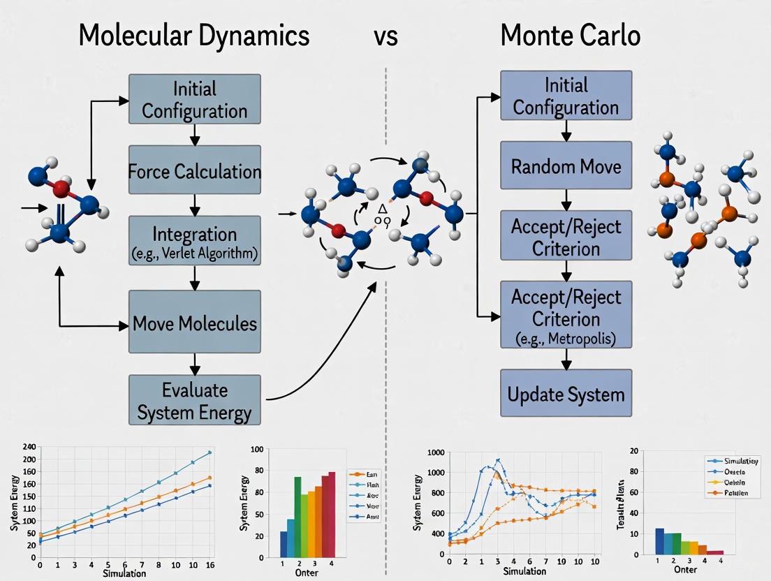
In computational chemistry and materials science, Molecular Dynamics (MD) and Monte Carlo (MC) simulations represent two foundational paradigms for investigating molecular systems. Their core distinction lies in their fundamental approach: MD is deterministic, based on numerical integration of classical equations of motion, while MC is stochastic, relying on random sampling to explore configuration space [1] [2]. This deterministic-stochastic dichotomy dictates their respective applications, strengths, and limitations. MD simulations are unparalleled for studying time-dependent phenomena and dynamic processes, providing actual trajectories of molecular motion over time [2]. In contrast, MC simulations excel at calculating equilibrium thermodynamic properties and sampling complex energy landscapes, though they do not provide real-time dynamical information [3] [2]. This guide provides an objective comparison of these methods, focusing on their performance in research applications, particularly in drug discovery and materials science, supported by experimental data and detailed methodologies.
Core Methodological Differences and Theoretical Foundations
The following table summarizes the fundamental differences between Molecular Dynamics and Monte Carlo methods.
Table 1: Fundamental Differences Between Molecular Dynamics and Monte Carlo Methods
| Feature | Molecular Dynamics (MD) | Monte Carlo (MC) |
|---|---|---|
| Fundamental Principle | Deterministic; solves Newton's equations of motion [2] | Stochastic; based on random sampling and probability distributions [2] |
| Time Evolution | Explicitly simulates time evolution, providing dynamic trajectories [2] | Does not involve real time; focuses on state space sampling [2] |
| Primary Output | Time series of coordinates and velocities; dynamic properties [2] | Set of sampled configurations; thermodynamic averages [2] |
| Key Applications | Protein folding, chemical reaction pathways, molecular docking [2] | Calculation of free energy, phase transitions, equilibrium constants [2] |
| Handling of Temperature | Controlled via thermostats (e.g., Berendsen, Nose-Hoover) [4] | Incorporated via acceptance criteria (e.g., Metropolis criterion) [2] |
| Algorithm Basis | Numerical integration (e.g., Velocity Verlet) with a time step [4] | Generation of random moves accepted/rejected based on energy change [2] |
The deterministic nature of MD means that, given an identical starting configuration and the same force field, an MD simulation will produce the same trajectory every time. It achieves this by calculating forces from a potential energy function and numerically integrating Newton's equations of motion to update atomic positions and velocities over a series of small time steps [2]. This process provides a direct link to dynamical properties.
Conversely, MC methods are inherently probabilistic. They explore the configuration space of a system by generating random changes (moves) to the current configuration. The core of many MC algorithms is the Metropolis criterion, where a newly generated configuration is accepted if it lowers the system's energy, or accepted with a probability proportional to the Boltzmann factor if it raises the energy [2]. This procedure ensures the system is sampled according to the desired thermodynamic ensemble (e.g., NVT or NPT), but it contains no information about the kinetics of the process.
Table 2: Comparative Advantages and Limitations in Research
| Aspect | Molecular Dynamics (MD) | Monte Carlo (MC) |
|---|---|---|
| Strengths | Provides detailed dynamic behavior and time evolution [2]; Reveals binding mechanisms and reaction pathways [2]; High precision in simulating real molecular motions [2] | High computational efficiency for large systems [2]; No time step limitation, can overcome energy barriers efficiently [2]; Lower dependence on initial structure [2] |
| Limitations | Extremely high computational cost for large systems/long timescales [2]; Results can be sensitive to initial structure and force field choice [2] | Cannot provide time-dependent or kinetic information [2]; May suffer from insufficient sampling if simulations are too short [2]; Relies on assumptions about system state [2] |
Experimental Protocols and Simulation Workflows
To ensure reproducibility and provide a clear framework for researchers, this section outlines standard protocols for implementing MD and MC simulations. Adherence to these methodologies is critical for generating reliable and comparable scientific data.
Molecular Dynamics Simulation Protocol
The following diagram illustrates the standard workflow for a typical Molecular Dynamics simulation.
Molecular Dynamics Simulation Workflow
Step 1: System Preparation. The initial 3D structure of the target molecule or complex is obtained from experimental sources (e.g., Protein Data Bank) or predicted structures (e.g., AlphaFold models) [5]. The system's protonation states and disulfide bonds are assigned correctly.
Step 2: Force Field Selection. An appropriate molecular mechanics force field (e.g., AMBER, CHARMM, OPLS) is selected to define the potential energy function, which includes bonded terms (bonds, angles, dihedrals) and non-bonded terms (van der Waals, electrostatic interactions) [6].
Step 3: Solvation and Neutralization. The system is placed in a simulation box (e.g., cubic, rhombic dodecahedron) and solvated with explicit water molecules (e.g., TIP3P, SPC/E models). Ions are added to neutralize the system and achieve a physiologically relevant ionic concentration [4].
Step 4: Energy Minimization. The system's energy is minimized using algorithms like steepest descent or conjugate gradient to remove bad contacts and steric clashes, resulting in a stable starting configuration for dynamics [4].
Step 5: System Equilibration. The system is gradually heated to the target temperature (e.g., 310 K for physiological conditions) using a thermostat (e.g., Berendsen, Nose-Hoover) in the NVT ensemble (constant Number of particles, Volume, and Temperature). This is followed by equilibration in the NPT ensemble (constant Number of particles, Pressure, and Temperature) using a barostat (e.g., Berendsen, Parrinello-Rahman) to achieve the correct density [4].
Step 6: Production Simulation. The equilibrated system is simulated for an extended period (nanoseconds to microseconds, depending on the system and scientific question) with a time step of typically 1-2 femtoseconds. Coordinates and velocities are saved at regular intervals for subsequent analysis [4] [2].
Step 7: Trajectory Analysis. The saved trajectory is analyzed to compute properties of interest, which may include root-mean-square deviation (RMSD) for structural stability, radius of gyration, hydrogen bonding patterns, distance measurements between residues, or free energy calculations using methods like MM/PBSA [2].
Monte Carlo Simulation Protocol
The following diagram illustrates the standard workflow for a typical Monte Carlo simulation.
Monte Carlo Simulation Workflow
Step 1: System and Ensemble Definition. The molecular system is defined, and the appropriate statistical mechanical ensemble is selected (e.g., canonical/NVT, isothermal-isobaric/NPT, or grand canonical/μVT ensemble) based on the properties of interest [2].
Step 2: Initial Configuration. An initial configuration of the system is generated, which could be a crystal structure, a random arrangement of molecules, or a structure taken from another simulation.
Step 3: Move Proposal. A random trial move is proposed to perturb the current configuration. Common moves include:
- Displacement: Translating a randomly selected molecule or atom by a small random vector.
- Rotation: Rotating a molecule around a randomly chosen axis by a random angle.
- Volume Change: For NPT ensemble simulations, randomly changing the simulation box volume.
- Particle Insertion/Deletion: For grand canonical (μVT) ensemble simulations, randomly inserting or deleting a molecule [2].
Step 4: Energy Calculation. The potential energy of the new trial configuration (Enew) is calculated and compared to that of the old configuration (Eold). The energy difference, ΔE = Enew - Eold, is computed.
Step 5: Acceptance Criterion. The Metropolis criterion is applied: if ΔE ≤ 0, the move is automatically accepted. If ΔE > 0, the move is accepted with probability Paccept = exp(-ΔE/kB T), where kB is Boltzmann's constant and T is the temperature. This is implemented by comparing Paccept to a random number uniformly distributed between 0 and 1 [2].
Step 6: Configuration Update. If the trial move is accepted, the new configuration becomes the current state. If rejected, the old configuration is retained and counted again in the averaging process.
Step 7: Sampling and Repetition. After the acceptance decision, the current configuration (whether new or old) is used to sample the properties of interest (e.g., energy, density, order parameters). Steps 3-6 are repeated for millions of iterations to ensure adequate sampling of the relevant regions of configuration space.
Step 8: Averaging and Analysis. Once the simulation is deemed to have converged and sufficient sampling has been achieved, thermodynamic properties are computed as averages over the sampled configurations. For example, the average energy ⟨U⟩ is a simple arithmetic mean of the energies of all sampled states [2].
Performance Comparison in Drug Discovery Applications
The distinct capabilities of MD and MC make them suitable for different stages of the drug discovery pipeline. The following table compares their performance across key application areas.
Table 3: Application-Based Performance Comparison in Drug Discovery
| Application | Molecular Dynamics (MD) Performance | Monte Carlo (MC) Performance |
|---|---|---|
| Virtual Screening | Computationally expensive for ultra-large libraries; used for refining top hits from docking [5] | Efficient for sampling binding poses and estimating binding affinities for a smaller set of candidates [6] |
| Binding Affinity Prediction | Good for relative binding free energies via alchemical methods (e.g., FEP); provides structural insights [6] | Excellent for absolute binding free energy calculations using methods like Free Energy Perturbation (FEP) with Monte Carlo sampling [6] |
| Target Flexibility & Conformational Sampling | Excellent for capturing full atomistic flexibility and dynamics; can reveal cryptic pockets via enhanced sampling [5] | Limited in sampling large-scale protein backbone motions; efficient for side-chain and ligand conformational sampling [2] |
| Solubility & Partition Coefficients | Less efficient due to slow diffusion in explicit solvent; requires long simulation times | Highly efficient for calculating thermodynamic properties like logP and solubility via statistical sampling [2] |
| ADMET Prediction | Can provide insights into specific metabolic reaction pathways via QM/MM-MD [6] | Effective for predicting bulk properties related to absorption and distribution [6] |
In structure-based drug design (SBDD), MD simulations have become crucial for addressing the challenge of target flexibility. Most molecular docking tools treat the protein as largely rigid, but proteins and ligands are highly flexible in solution [5]. Advanced MD techniques, such as accelerated MD (aMD), smooth the system's potential energy surface, decreasing energy barriers and accelerating transitions between different low-energy states. This allows for more efficient sampling of distinct biomolecular conformations and helps identify cryptic pockets not visible in the original crystal structure [5]. The Relaxed Complex Method (RCM) is a notable approach that uses representative target conformations from MD simulations, including those with novel cryptic binding sites, for subsequent docking studies [5].
MC methods, particularly those employing Free Energy Perturbation (FEP) with Monte Carlo sampling, offer a rigorous theoretical framework for calculating binding free energy changes [6]. This is crucial for lead optimization, where small chemical modifications are made to improve a compound's affinity and specificity. FEP/MC calculations can predict the relative binding free energies between related compounds with high accuracy, guiding medicinal chemists toward more potent analogs.
Hybrid Methods and Advanced Integration
Recognizing that neither MD nor MC is universally superior, researchers often combine them to leverage their respective strengths. These hybrid approaches are particularly powerful for simulating complex biomolecular processes.
Table 4: Overview of Hybrid MD-MC Methods
| Hybrid Method | Description | Key Applications |
|---|---|---|
| Replica Exchange MD (REMD) | Multiple MD simulations run in parallel at different temperatures, with periodic exchange of configurations based on a Metropolis-like criterion [2] | Protein folding, studying thermodynamic behavior of large molecular systems, enhanced sampling [2] |
| Meta-Dynamics | An external history-dependent bias potential is added to the Hamiltonian to discourage the system from revisiting already sampled states, effectively accelerating the escape from local energy minima [2] | Free energy calculations, exploring chemical reaction paths, and studying complex conformational changes [2] |
| MC-Assisted Free Energy Calculations | MD simulations provide dynamic trajectories, while MC sampling is used to calculate free energy differences and binding affinities with high efficiency [6] | Drug design optimization, calculating binding affinities in complex systems [6] |
The following diagram illustrates how MD and MC are integrated in a hybrid approach for advanced sampling.
Hybrid MD-MC Sampling Strategy
These hybrid methods are widely applied in drug design, materials science, and protein folding research. In drug design, MD simulations reveal dynamic interactions between drug candidates and their target proteins, while MC simulations help calculate binding free energies and optimize candidate structures [2]. In materials science, MD simulations study mechanical properties and time-dependent behavior, while MC simulations calculate thermodynamic properties like phase transitions [2].
Successful implementation of MD and MC simulations requires both specialized software and access to computational resources. The following table details key solutions used in the field.
Table 5: Essential Research Reagents and Computational Resources
| Resource Type | Examples | Function and Application |
|---|---|---|
| MD Simulation Software | AMS [4], GROMACS, NAMD, LAMMPS, AMBER, CHARMM | Software packages that perform molecular dynamics simulations using various force fields and integration algorithms [4]. |
| MC Simulation Software | Various specialized MC packages, ProtoMS, MCCCS Towhee | Software designed for Monte Carlo sampling, often with specific capabilities for free energy calculations [2]. |
| Force Fields | AMBER, CHARMM, OPLS-AA, GAFF | Parameter sets defining potential energy functions, including bonded and non-bonded interactions, for different classes of molecules [6]. |
| Enhanced Sampling Tools | PLUMED [4], Meta-Dynamics [2] | Plugins and algorithms that enhance the sampling of rare events and calculate free energies. |
| Quantum Chemistry Data | Open Molecules 2025 (OMol25) dataset [7] | Large-scale DFT datasets used to train Machine Learned Interatomic Potentials (MLIPs) for more accurate force fields [7]. |
| High-Performance Computing | Cloud computing (e.g., AWS, Google Cloud), GPU clusters [5] | Essential computational resources for handling ultra-large virtual screenings and long timescale simulations [5]. |
The recent release of massive computational datasets like Open Molecules 2025 (OMol25), which contains over 100 million 3D molecular snapshots with properties calculated using Density Functional Theory (DFT), is revolutionizing the field [7]. Such datasets are used to train Machine Learned Interatomic Potentials (MLIPs), which can provide DFT-level accuracy at a fraction of the computational cost, thereby enhancing both MD and MC simulations [7].
Molecular Dynamics and Monte Carlo simulations represent two powerful but philosophically distinct paradigms for computational research. MD's deterministic nature provides unparalleled insights into time-dependent processes and molecular mechanisms, making it indispensable for studying dynamics, folding, and binding pathways. MC's stochastic approach offers superior efficiency for calculating thermodynamic equilibrium properties and free energies. The choice between them is not a matter of which is better, but which is more appropriate for the specific scientific question at hand. Furthermore, the growing trend of hybrid methods, which leverage the strengths of both approaches, alongside the integration of machine-learning potentials trained on massive quantum chemical datasets, points toward a future where the boundaries between these paradigms become increasingly blurred, leading to more comprehensive and predictive computational models in drug discovery and materials science.
In the quest to understand and predict the behavior of molecular systems, from drug molecules interacting with their protein targets to the self-assembly of complex materials, researchers rely on computational methods to navigate the intricate energy landscapes that govern molecular stability and function. An energy landscape is a conceptual mapping of all possible configurations of a molecular system against their corresponding energy levels. Within this landscape, low-energy valleys represent stable states, while high-energy peaks represent barriers to change. Two powerful computational techniques dominate this exploration: Molecular Dynamics (MD) and Monte Carlo (MC). Though sometimes used to address similar problems, their fundamental approaches are philosophically and technically distinct. MD simulation is a deterministic method that produces a time-evolving narrative of atomic motion, effectively creating a movie of molecular life [1] [8]. In contrast, MC simulation is a probabilistic method that generates a statistical collection of snapshots, focusing on the system's equilibrium properties without reference to a temporal dimension [1] [2]. This guide provides an objective comparison of how these two methods are used to explore energy landscapes, detailing their performance, supported by experimental data and protocols.
Core Principles: Dynamics vs. Sampling
The Molecular Dynamics (MD) Approach
MD simulation predicts the trajectory of a molecular system by numerically solving Newton's equations of motion for every atom in the system [8] [2]. The core principle is that by knowing the forces acting on each atom (calculated from a molecular mechanics force field) and the initial atomic positions and velocities, one can determine the acceleration, and subsequently update the positions and velocities over a series of very short time steps (femtoseconds, 10⁻¹⁵ s) [8] [9]. This results in a time-series of atomic coordinates—a trajectory—that captures the dynamic evolution of the system, including its fluctuations and rare events, as it navigates its energy landscape [9].
The Monte Carlo (MC) Approach
MC simulation, in its most common form for molecular systems, explores the energy landscape through random sampling of configurations [10] [2]. Unlike MD, it is not based on classical mechanics and does not model the physical pathway between states. Instead, it generates new random configurations that are then accepted or rejected based on a probabilistic criterion (e.g., the Metropolis criterion) designed to ensure that the ensemble of sampled configurations conforms to the desired statistical distribution, such as the Boltzmann distribution for a canonical ensemble [11]. The primary output is therefore not a trajectory, but a set of statistically independent configurations used to compute equilibrium thermodynamic averages [2].
Table 1: Foundational Differences Between MD and MC
| Feature | Molecular Dynamics (MD) | Monte Carlo (MC) |
|---|---|---|
| Theoretical Basis | Classical (Newtonian) mechanics [8] | Statistics and probability theory [10] |
| Time Evolution | Explicitly simulated [2] | Not simulated [2] |
| Primary Output | Trajectory (time-series of coordinates) [9] | Set of uncorrelated configurations [2] |
| Key Controlled Variables | Energy, Volume, Number of atoms (NVE) or Temperature (NVT) or Pressure (NPT) [12] | Temperature, Chemical Potential, Volume (μVT) or others, depending on ensemble [11] |
| Nature of Method | Deterministic [1] | Stochastic (Probabilistic) [1] |
Comparative Performance: Quantitative and Qualitative Analysis
The choice between MD and MC has profound implications for the type of information a researcher can extract. Their performance differs significantly across various types of analysis.
Observable Properties and Performance
MD is unparalleled for calculating properties that are inherently time-dependent. The analysis of the Mean Squared Displacement (MSD) of atoms or molecules over time allows for the direct calculation of transport properties like the diffusion coefficient [9]. Similarly, time correlation functions from MD trajectories can be used to determine rates and spectroscopic properties. In material science, MD can simulate the direct application of strain to a system and calculate the resulting stress, enabling the computation of mechanical properties like Young's modulus from a stress-strain curve [9].
MC, by contrast, excels at calculating thermodynamic equilibrium properties and free energies [2]. Because it can efficiently sample phase space without being trapped by energy barriers in the same way as MD (through the use of specialized moves), it is often the method of choice for studying phase transitions, determining solubility parameters, and calculating binding affinities in drug design by estimating the free energy of binding [2].
Table 2: Comparison of Observable Properties and Computational Performance
| Analysis Type | Molecular Dynamics (MD) | Monte Carlo (MC) |
|---|---|---|
| Time-dependent Phenomena | Excellent (e.g., protein folding, diffusion, kinetics) [8] [9] | Not Applicable [2] |
| Thermodynamic Properties | Possible, but may be inefficient for large barriers | Excellent (e.g., free energy, phase equilibrium) [2] |
| Mechanical Properties | Directly calculable (e.g., via stress-strain curves) [9] | Not directly accessible |
| Handling Energy Barriers | Can be inefficient (requires waiting for rare events) | More efficient with specialized moves (e.g., configurational bias) |
| Inherent Parallelizability | Highly parallelizable (e.g., across atoms, spatial domains) [9] | Difficult to parallelize [1] |
| Typical System Constraints | Atoms must be freely movable (off-lattice) [1] | Can simulate both on-lattice and off-lattice models |
Experimental Data and Validation
The validation of both methods often comes from comparing their results with experimental data. For instance, MD simulations have been extensively used to study asphalt materials. In one such study, MD was used to calculate the cohesive energy density of an asphalt model, which was then used to derive the solubility parameter, a key thermodynamic property used to predict compatibility between materials. The simulation result was found to be in close agreement with experimental values, validating the model and the method [12].
In the field of pharmacometrics, a study evaluated the performance of a Monte Carlo Parametric Expectation Maximization (MC-PEM) algorithm, a specific MC-type method used for complex mechanistic models in drug development. The study involved a model with 45 estimated parameters and 14 differential equations. The results demonstrated that the MC-PEM algorithm provided unbiased and precise parameter estimates, with the median estimated-to-true value ratio for model parameters being 1.01 for rich data sampling, demonstrating high accuracy and robustness even with poor initial estimates [13].
Methodological Deep Dive: Protocols and Workflows
A Standard MD Workflow
The following diagram illustrates the typical, iterative workflow of an MD simulation, from initial setup to final analysis.
Detailed MD Protocol:
- Prepare Initial Structure: The simulation begins with a starting atomic configuration, often obtained from experimental sources like the Protein Data Bank (PDB) for biomolecules or crystal structure databases for materials [9]. Missing atoms or regions may need to be modeled.
- System Initialization: Initial velocities are assigned to every atom, typically sampled from a Maxwell-Boltzmann distribution corresponding to the desired simulation temperature [9].
- Force Calculation: This is the most computationally intensive step. The forces acting on each atom are calculated based on a molecular mechanics force field, which is a mathematical model describing the potential energy of the system as a sum of terms for bonds, angles, dihedrals, and non-bonded interactions (van der Waals and electrostatics) [8] [9].
- Time Integration: The forces are used to numerically integrate Newton's equations of motion. Algorithms like the Verlet or leap-frog algorithm are commonly used due to their stability and good energy conservation properties over long simulations. This step updates the atomic positions and velocities for the next time step (e.g., 1-2 femtoseconds) [9].
- Trajectory Analysis: The raw output of atomic coordinates over time (the trajectory) is analyzed to compute properties of interest, such as radial distribution functions, diffusion coefficients, or root-mean-square deviation (RMSD) of a protein structure [9].
A Standard MC Workflow
The following diagram illustrates the workflow of a typical Metropolis-based Monte Carlo simulation, highlighting its stochastic, cycle-based nature.
Detailed MC Protocol:
- Generate Initial Configuration: The simulation starts with an initial molecular configuration.
- Perturb Configuration: A random change is made to the system. This could be the displacement of a randomly chosen atom, a rotation around a chemical bond, or even a more complex move like swapping particles [11].
- Calculate Energy Change: The energy of the new, perturbed configuration (Enew) is calculated and compared to the energy of the previous configuration (Eold). The energy difference, ΔE = Enew - Eold, is computed.
- Metropolis Criterion: This stochastic step determines whether the new configuration is accepted and becomes the current state, or is rejected, in which case the old configuration is recounted.
- If ΔE ≤ 0, the new, lower-energy configuration is always accepted.
- If ΔE > 0, the new, higher-energy configuration is accepted with a probability of exp(-ΔE/kBT), where kB is the Boltzmann constant and T is the temperature [11]. This criterion ensures that the sampling converges to the Boltzmann distribution.
- Sample Configuration: If the move is accepted, the new configuration becomes the current state. Regardless of acceptance or rejection, the current configuration (or its properties) is added to the running averages being computed.
- Iterate: Steps 2-5 are repeated for millions of cycles until the thermodynamic averages of interest (e.g., average energy, pressure) have converged.
The Scientist's Toolkit: Essential Research Reagents and Materials
Successful implementation of MD and MC simulations requires a suite of software and computational "reagents." The table below details key resources for different stages of the workflow.
Table 3: Essential Research Reagents and Computational Tools
| Item Name | Function/Brief Explanation | Relevance to MD/MC |
|---|---|---|
| Force Fields (e.g., CHARMM, AMBER, OPLS) | Mathematical models that define the potential energy surface and interatomic forces. They include parameters for bonds, angles, and non-bonded interactions. | Critical for both [12] [8] |
| Molecular Dynamics Software (e.g., GROMACS, NAMD, LAMMPS, AMBER, Desmond) | Specialized software packages that implement the algorithms for MD simulation, including force calculation, integration, and parallelization. | Primarily MD [8] |
| Monte Carlo Software (e.g., Cassandra, Towhee, MC Packages in LAMMPS) | Software designed to perform MC simulations, often with a library of available "moves" for different types of molecules and ensembles. | Primarily MC |
| Structure Visualization (e.g., VMD, PyMol) | Tools to visualize initial structures, analyze simulation trajectories, and render molecular graphics for publication. | Critical for both |
| Trajectory Analysis Tools (e.g., MDTraj, GROMACS tools) | Scripts and software modules for analyzing simulation outputs to compute properties like RMSD, RDF, MSD, and more. | Primarily MD |
| High-Performance Computing (HPC) / GPUs | Central Processing Units (CPUs), and especially Graphics Processing Units (GPUs), provide the massive computational power required for simulations of biologically relevant timescales and system sizes. | Critical for both [8] [9] |
Molecular Dynamics and Monte Carlo are complementary, not competing, tools in the computational scientist's arsenal. The decision to use one over the other is not a matter of which is "better," but which is more appropriate for the specific research question.
- Choose Molecular Dynamics when the research goal requires understanding time-dependent behavior, kinetic pathways, or transport properties. MD is the definitive choice for simulating processes like protein folding, ligand binding kinetics, ion diffusion through a channel, or the mechanical response of a material to deformation [9] [2].
- Choose Monte Carlo when the primary interest is in equilibrium thermodynamic properties, such as free energy, phase equilibria, or binding affinity. MC is often more efficient for sampling complex energy landscapes with high barriers and is inherently suited for studying systems at a defined chemical potential [2].
Furthermore, the lines between these methods are increasingly blurred by the development of hybrid techniques. Methods like Replica Exchange MD (REMD) incorporate MC-like temperature swaps between parallel MD simulations to enhance sampling [2]. Similarly, Meta-Dynamics adds a history-dependent bias to MD to push the system away from already-visited states, achieving more efficient exploration akin to MC [2]. The astute researcher will select the core methodology based on their primary objective while leveraging these advanced hybrids to overcome the inherent limitations of any single technique.
Molecular Dynamics (MD) and Monte Carlo (MC) simulations are foundational techniques in computational chemistry and materials science. While both methods aim to sample the configurations of a system, their underlying principles dictate the specific observables they can efficiently and naturally compute. MD simulations generate a time-evolving trajectory by numerically integrating Newton's equations of motion, making them uniquely suited for calculating time-dependent properties. In contrast, MC simulations generate a sequence of states through stochastic moves designed to sample from a specific statistical ensemble (e.g., NVT, NPT), making them highly efficient for determining equilibrium thermodynamic properties. This guide provides a structured comparison of the performance and applications of these two methods, focusing on the distinct types of observables they are best equipped to handle.
Comparative Analysis of Key Observables
The table below summarizes the core observables accessible through MD and MC simulations, highlighting the inherent strengths of each method.
Table 1: Key Observables Accessible via Molecular Dynamics and Monte Carlo Simulations
| Observable Category | Specific Observable | Primary Method | Performance & Notes |
|---|---|---|---|
| Time-Dependent/Dynamic Properties | Diffusion Coefficient | MD | Directly calculated from Mean Squared Displacement (MSD) over time [14]. |
| Viscosity | MD | Computed from stress-tensor autocorrelation functions [14]. | |
| Reaction Rates | MD | Derived from time-correlation functions or by measuring transition times between states [14]. | |
| Relaxation Rates (NMR) | MD | Obtained from autocorrelation functions of spin vectors or dipolar interactions [14]. | |
| Thermal Conductivity | MD | Calculated from heat current autocorrelation functions (Green-Kubo relation) [14]. | |
| Equilibrium Thermodynamic Properties | Enthalpy of Vaporization | MC / MD | Both can calculate, but MC often reaches equilibrium faster; can be used for force field training [14]. |
| Radial Distribution Function | MC / MD | Both can compute this structural property; MC can be more efficient for dense systems [14]. | |
| Phase Diagrams | MC | Highly efficient for determining phase coexistence conditions (e.g., via Gibbs Ensemble MC) [15]. | |
| Free Energy Differences | MC | Specialized methods (e.g., Free Energy Perturbation, Umbrella Sampling) are often implemented in MC. | |
| Potential Energy | MC / MD | A fundamental output of both simulations; MC excels at sampling the configurational energy. |
Methodological Protocols and Workflows
The computational workflow for extracting these observables differs significantly between MD and MC, as illustrated in the following diagram.
Protocol for Calculating Time-Dependent Properties with MD
The power of MD for dynamic properties is exemplified by calculating a self-diffusion coefficient, a key observable inaccessible to standard MC.
- System Setup: Construct the atomic system (e.g., 895 water molecules in a periodic box [14]) and assign initial velocities from a Maxwell-Boltzmann distribution.
- Equilibration: Run an initial MD simulation in the NVT (canonical) or NPT (isothermal-isobaric) ensemble to stabilize temperature and density. Thermostats (e.g., Nosé-Hoover) and barostats are applied here.
- Production Run: Perform a long MD simulation in the NVE (microcanonical) or NVT ensemble, saving atomic coordinates at regular intervals (e.g., every 1-10 fs for water).
- Trajectory Analysis:
- For each atom i, calculate the Mean Squared Displacement (MSD) as a function of time: ( \text{MSD}(t) = \langle | \vec{r}i(t) - \vec{r}i(0) |^2 \rangle ), where the angle brackets denote an average over all atoms and time origins.
- The self-diffusion coefficient D is obtained from the Einstein relation: ( D = \frac{1}{6} \lim_{t \to \infty} \frac{d}{dt} \text{MSD}(t) ).
- Validation: The calculated D can be compared directly to experimental measurements, such as pulsed-field gradient NMR data, and used to top-down train force fields via methods like reversible simulation [14].
Protocol for Calculating Thermodynamic Properties with MC
The efficiency of MC for thermodynamics is demonstrated by calculating an enthalpy of vaporization ((\Delta H_{vap})), a critical equilibrium property.
- System Definition: Define the system in a specific ensemble (e.g., NVT for a liquid). No initial velocities are needed.
- Sampling: Use the Metropolis-Hastings algorithm to generate new configurations. A typical move is randomly displacing a single atom. The move is accepted with probability ( P{accept} = \min(1, e^{-\beta \Delta U}) ), where ( \Delta U ) is the change in potential energy and ( \beta = 1/kB T ). This ensures sampling from the Boltzmann distribution.
- Equilibration: Discard an initial number of steps until the potential energy fluctuates around a stable average, indicating equilibrium has been reached.
- Ensemble Averaging:
- The enthalpy of vaporization is calculated using the thermodynamic definition: ( \Delta H{vap} = \langle E{gas} \rangle - \langle E_{liquid} \rangle + RT ), where ( \langle E \rangle ) is the average potential energy per molecule from separate simulations of the gas and liquid phases.
- The Radial Distribution Function (RDF), ( g(r) ), is calculated by averaging the histogram of interatomic distances over the entire MC ensemble [14].
- Application: These averaged properties are central to the parameterization and validation of force fields, as done in tools like ForceBalance [14] and for studying phase equilibria in complex alloys [15].
The Scientist's Toolkit: Essential Research Reagents
The table below lists key computational "reagents" and software essential for conducting research in this field.
Table 2: Key Research Reagents and Software Solutions
| Tool Name | Type/Function | Key Application in MD/MC Research |
|---|---|---|
| GROMACS [16] | MD Simulation Software | High-performance MD package used for simulating biomolecular systems and calculating dynamic trajectories. |
| Rosetta Backrub [16] | Monte Carlo Algorithm | Models backbone flexibility in proteins based on high-resolution crystal structures; used for conformational sampling. |
| ForceBalance [14] | Force Field Optimization Tool | An ensemble reweighting method used to automatically parameterize force fields against experimental data. |
| DeePMD-kit [17] | Machine Learning Interatomic Potential | Framework for building and running ML-based potentials, enabling accurate and large-scale MD simulations. |
| Reversible Simulation [14] | Differentiable Simulation Method | A memory-efficient approach to train force fields (both classical and ML-based) to match experimental data, including dynamic observables. |
| Maximum Entropy Reweighting [18] | Integrative Analysis Protocol | A robust procedure to combine MD simulations with experimental data (e.g., NMR, SAXS) to determine accurate conformational ensembles of biomolecules like IDPs. |
| Machine Learning Interatomic Potentials (ML-IAPs) [17] [19] | Advanced Force Fields | Data-driven potentials (e.g., MACE, NequIP) that offer near-ab initio accuracy with the computational efficiency of classical MD, expanding the scope of both MD and MC studies. |
MD and MC are complementary, not competing, techniques. The choice between them is dictated by the scientific question. MD is indispensable for investigating kinetics, transport, and any time-dependent phenomenon, providing a direct window into dynamical processes. MC is the tool of choice for high-efficiency sampling of equilibrium thermodynamics, including free energies and phase behavior. Modern research increasingly leverages their synergies, using MC-generated ensembles as initial states for MD or using ML-potentials trained on ab initio data to enhance the accuracy of both methods. Understanding their distinct strengths, as outlined in this guide, is fundamental for designing robust computational studies in chemistry, materials science, and drug development.
In computational science, Molecular Dynamics (MD) and Monte Carlo (MC) simulations represent two foundational pillars for studying complex molecular systems. While they can sometimes be used to answer similar scientific questions, their underlying mathematical frameworks and operational principles are fundamentally different. MD is fundamentally rooted in the deterministic principles of Hamiltonian and Lagrangian mechanics, tracing physical trajectories through time by numerically solving Newton's equations of motion. In contrast, MC methods, with the Metropolis algorithm at their core, rely on stochastic sampling to generate configurations according to a desired probability distribution, making no attempt to model physical dynamics [20].
This guide provides a comprehensive, objective comparison of these methodologies. It examines their theoretical foundations, computational performance, hardware requirements, and practical implementation to assist researchers, scientists, and drug development professionals in selecting the most appropriate technique for their specific research challenges.
The mathematical engines driving MD and MC are distinct, leading to different strengths and application domains.
Molecular Dynamics: Deterministic Dynamics
Molecular Dynamics simulations are governed by classical mechanics:
- Lagrangian Mechanics: The Lagrangian framework, defined as ( L = T - V ) (where ( T ) is kinetic energy and ( V ) is potential energy), is used to derive the equations of motion via the Euler-Lagrange equation. This approach is particularly powerful in handling constraints.
- Hamiltonian Mechanics: The Hamiltonian, ( H = T + V ), represents the total energy of the system. Hamilton's equations describe the evolution of the system's coordinates and momenta in phase space, forming the basis for many integration algorithms, including those that conserve energy.
These frameworks ensure that MD simulations follow a physically-realistic path, providing access to dynamic properties and non-equilibrium processes [20].
Monte Carlo: Stochastic Sampling
The Metropolis-Hastings algorithm, a workhorse of MC simulations, enables sampling from complex probability distributions (like the Boltzmann distribution) without requiring physical dynamics:
- A random move is proposed from the current state to a new state.
- The energy change (( \Delta E )) between the states is computed.
- The move is accepted with a probability ( \min(1, e^{-\Delta E / k_B T}) ).
This stochastic process ensures detailed balance and, for ergodic systems, generates a sequence of states that correctly samples the equilibrium distribution. A key advantage is that the proposed moves need not follow a physically allowed process, which can be exploited to accelerate sampling through techniques like cluster moves or configuration bias [20].
Conceptual Workflows
The diagram below illustrates the fundamental operational difference between the MD and MC workflows.
Performance and Hardware Benchmarking
The computational characteristics of MD and MC differ significantly, influencing hardware choices and cost-effectiveness.
Molecular Dynamics Performance
MD simulations are highly computationally intensive and have been extensively optimized for modern hardware, particularly GPUs. The table below summarizes benchmark data for popular MD software running on different hardware configurations.
Table 1: Benchmark performance of MD software on various hardware (system: T4 Lysozyme, ~44,000 atoms) [21] [22].
| MD Software | Hardware Configuration | Performance (ns/day) | Key Considerations |
|---|---|---|---|
| OpenMM | NVIDIA H200 (GPU) | 555 ns/day | Peak performance, ideal for time-critical projects [22]. |
| OpenMM | NVIDIA L40S (GPU) | 536 ns/day | Best value, excellent cost-efficiency [22]. |
| OpenMM | NVIDIA T4 (GPU) | 103 ns/day | Budget option, slower but low hourly cost [22]. |
| GROMACS | Multi-GPU (e.g., 2x A100) | Varies by system | Good strong scaling for large systems; requires -nb gpu -pme gpu -update gpu flags [21]. |
| AMBER (PMEMD) | Single GPU (e.g., V100) | Varies by system | A single simulation typically does not scale beyond 1 GPU [21]. |
| NAMD 3 | Multi-GPU (e.g., 2x A100) | Varies by system | Good scaling; uses namd3 +p<CPUs> +idlepoll for execution [21]. |
Monte Carlo Performance and Efficiency
MC performance is less about raw speed and more about sampling efficiency, measured by how effectively a Markov chain explores the configuration space and converges to the equilibrium distribution. Advanced algorithms are crucial for tackling complex, high-dimensional problems.
Table 2: Advanced MCMC algorithms for improving sampling efficiency [23] [24].
| Algorithm | Key Mechanism | Advantages | Typical Application Context |
|---|---|---|---|
| Adaptive Metropolis (AM) | Recursively updates proposal covariance using the entire sampling history [23]. | Improves global exploration; asymptotic convergence guarantees [23]. | General-purpose Bayesian inverse problems. |
| DREAM (Differential Evolution Adaptive Metropolis) | Uses genetic algorithm-inspired mechanisms and multiple parallel chains [23]. | Efficiently traverses high-dimensional and multimodal posteriors [23]. | Complex hydrogeological inversions, tall panel datasets. |
| CMAM (Covariance Matrix Adaptation Metropolis) | Integrates population-based CMA-ES optimization with Metropolis sampling [23]. | Dynamically adjusts proposal orientation and scale; robust convergence [23]. | High-dimensional, multimodal Bayesian inverse problems. |
| ASIS (Ancillarity-Sufficiency Interweaving Strategy) | Alternates between sufficient (centered) and ancillary (non-centered) parameterizations [24]. | Alleviates correlation between parameters (e.g., random & fixed effects); optimal convergence rate [24]. | Bayesian hierarchical panel data models. |
Hardware and Cost Analysis
Choosing the right hardware is critical for computational efficiency. The following diagram and table outline key considerations and recommendations.
Table 3: Hardware selection guide for MD and large-scale MC simulations [25] [26] [22].
| Component | Recommendation | Rationale & Notes |
|---|---|---|
| GPU for MD | NVIDIA RTX 4090 / 5090 or L40S (cost-effective); H200 (peak performance) [25] [22]. | MD codes (GROMACS, AMBER, NAMD) use mixed precision, where consumer GPUs excel. L40S offers the best cost-efficiency, while H200 is fastest [26] [22]. |
| GPU for FP64 Workloads | NVIDIA A100/H100 (Data Center GPUs) [26]. | Some quantum chemistry/MC codes require strong double-precision (FP64) throughput, which is limited on consumer GPUs [26]. |
| CPU | AMD Threadripper PRO or Intel Xeon Scalable Processors [25]. | Prioritize clock speeds over core count for many MD workloads. Dual CPU setups are viable for workloads requiring very high core counts or RAM [25]. |
| RAM | Minimum 4GB per CPU core; scale with system size [21]. | Essential for handling large molecular systems and trajectory data. |
| Cost Metric | €/ns/day for MD; Cost per result for other simulations [26]. | Enables objective comparison between cloud and on-premise hardware. Benchmark a small case first [26] [22]. |
Experimental Protocols and Methodologies
Reproducibility is paramount. Below are detailed protocols for running benchmarks and ensuring sampling efficiency.
Molecular Dynamics Simulation Protocol
A standard MD benchmark protocol for a protein-ligand system in explicit solvent involves the following stages. The specific commands are for GROMACS but are analogous in other packages like AMBER and NAMD [21].
- System Preparation: Obtain a protein structure from the PDB (e.g., 4W52). Use a tool like
pdb2gmxto generate topology and assign a force field. Solvate the protein in a water box (e.g., TIP3P) and add ions to neutralize the system's charge. Energy Minimization: Run a steepest descent algorithm to remove steric clashes.
Equilibration:
- NVT Ensemble: Equilibrate the system at a constant temperature (e.g., 300 K) for 100 ps, restraining heavy atom positions.
- NPT Ensemble: Equilibrate at constant pressure (1 bar) for 100 ps, with restraints on heavy atoms.
Production Run: Run an unrestrained simulation. The following example shows a GPU-accelerated GROMACS run. The number of steps (e.g.,
-nsteps 50000) defines the simulation length.Performance Analysis: The key output is the simulation throughput in nanoseconds per day (ns/day). This is calculated by the software and reported in the log file.
Monte Carlo Sampling Efficiency Protocol
Assessing the quality of an MCMC simulation is different from MD. The focus is on convergence and sampling quality.
- Algorithm Selection: Choose a sampler appropriate for the problem (e.g., Adaptive Metropolis for simple problems; DREAM or CMAM for high-dimensional/multimodal posteriors) [23].
- Chain Initialization: Run multiple (e.g., 4-8) chains from dispersed starting points to diagnose convergence.
- Convergence Diagnostics: Monitor the Gelman-Rubin statistic ((\hat{R})), which compares within-chain and between-chain variance. (\hat{R} \leq 1.05) for all parameters indicates convergence.
- Efficiency Metrics:
- Effective Sample Size (ESS): Calculate the ESS for each parameter, which estimates the number of independent samples. Higher is better.
- Integrated Autocorrelation Time: Measures the number of steps needed to get an independent sample. Lower is better.
- Reproducibility: For both MD and MC, always record a "run card": a text file with the exact input parameters, software versions, CPU/GPU models, and seed values for stochastic elements [26].
The Scientist's Toolkit
This section details essential software and hardware resources for conducting MD and MC research.
Table 4: Key research tools and resources for MD and MC simulations.
| Tool / Resource | Function / Purpose | Examples & Notes |
|---|---|---|
| MD Simulation Engines | Software to perform the numerical integration of equations of motion. | GROMACS, AMBER, NAMD, LAMMPS, OpenMM [21] [22]. |
| MC Simulation Software | Software for stochastic sampling and risk analysis. | Stand-alone: Analytica, GoldSim. Excel add-ins: @RISK, Analytic Solver, ModelRisk [27]. |
| Force Fields | Mathematical models describing interatomic potentials. | AMBER, CHARMM, OPLS. Define the "rules" of interaction for MD. |
| System Preparation Tools | Prepare molecular structures for simulation. | PDB2GMX (GROMACS), tleap (AMBER), CHARMM-GUI. |
| Visualization & Analysis | Analyze trajectories and simulation outputs. | VMD, Chimera, MDAnalysis, GROMACS analysis tools. |
| High-Performance Computing (HPC) | Hardware for running simulations in a reasonable time. | GPUs: NVIDIA A100, H100, RTX 4090, L40S. CPUs: AMD Threadripper, Intel Xeon [25] [22]. |
| Optimization & Sampling Enhancers | Advanced algorithms to improve convergence and efficiency. | For MC: Adaptive MCMC, DREAM, CMAM, ASIS [23] [24]. For MD: Hydrogen mass repartitioning (enables 4 fs timesteps) [21]. |
Molecular Dynamics and Monte Carlo methods are powerful yet distinct computational frameworks. The choice between them should be guided by the specific scientific question.
- Choose Molecular Dynamics when investigating time-dependent phenomena, dynamic processes, transport properties, or non-equilibrium systems. Its foundation in Hamiltonian/Lagrangian mechanics provides a physically intuitive path for studying how systems evolve.
- Choose Monte Carlo methods when the primary goal is efficient equilibrium sampling, computing thermodynamic averages, or navigating complex, high-dimensional landscapes. The Metropolis algorithm and its modern adaptive extensions excel at generating statistically rigorous ensembles without the overhead of simulating dynamics.
Modern research often leverages the strengths of both methods, and the ongoing development of more efficient algorithms and powerful, cost-effective hardware like the NVIDIA L40S GPU continues to push the boundaries of what is possible in computational molecular science.
Practical Implementation and Key Applications in Biomolecular Simulation and Drug Design
Molecular Dynamics (MD) and Monte Carlo (MC) simulations are foundational techniques for studying molecular behavior and interactions. The core distinction lies in their fundamental approach: MD is a deterministic method that tracks the time evolution of a system by solving equations of motion, providing detailed insights into dynamic processes like protein folding or chemical reactions. In contrast, MC is a probabilistic method that explores the state space of a system through random sampling, making it ideal for calculating thermodynamic equilibrium properties such as free energy and phase transitions [1] [2]. This guide provides a detailed, step-by-step comparison of their operational procedures, supported by experimental data and protocols.
Core Algorithmic Walkthroughs
A Typical Molecular Dynamics Time-Step
Molecular Dynamics simulations numerically simulate the motion of atoms and molecules over time. The following workflow outlines the sequential steps executed for every time-step in an MD simulation, typically on the order of femtoseconds (10⁻¹⁵ seconds).
Step 1: Force Calculation The simulation calculates the net force Fᵢ acting on each atom i in the system. This is typically derived from a force field, which is a mathematical model of the interatomic potential energy U(rᴺ). The force is the negative gradient of this potential: Fᵢ = -∇ᵢU. This calculation is often the most computationally intensive part of the time-step, as it involves evaluating all non-bonded interactions (e.g., Lennard-Jones and Coulombic potentials) [21]. For large systems, techniques like Particle Mesh Ewald (PME) are used to handle long-range electrostatic interactions efficiently [22].
Step 2: Integration of Equations of Motion Using the calculated forces, the simulation integrates Newton's equations of motion, Fᵢ = mᵢaᵢ, to update the atomic velocities and positions. Common integration algorithms include the Verlet and Leap-frog methods. This step determines the new state of the system a short time (the time-step, Δt) later. The choice of Δt is critical for stability and is often limited to 1-2 femtoseconds, though can be extended to 4 fs with techniques like hydrogen mass repartitioning [21].
Step 3: Update Positions and Velocities The integrator yields new atomic positions and velocities. In modern MD software, this "update and constraints" step can be offloaded to a GPU for better performance, especially when the GPU is fast relative to the CPU [28]. Constraints, often applied to bonds involving hydrogen atoms, are enforced using algorithms like LINCS or SHAKE to allow for a larger time-step.
Step 4: Data Output Finally, relevant data for the current time-step—such as atomic coordinates (trajectory), energies, and temperatures—are written to output files. To avoid I/O becoming a significant bottleneck, trajectory frames are saved at intervals (e.g., every 1,000-10,000 steps) rather than at every step [22].
A Typical Monte Carlo Move
Monte Carlo simulations generate a sequence of system configurations (or "microstates") through random moves, with the goal of sampling from a desired statistical ensemble, such as the canonical (NVT) ensemble. The following workflow outlines the procedure for a single Monte Carlo "move."
Step 1: System Perturbation A trial move is generated by randomly perturbing the current configuration of the system. In a simulation of molecules in a box, a common move is to randomly select a single particle and displace it by a small, random vector. The size of this displacement is a tunable parameter that can affect the simulation's efficiency [2].
Step 2: Energy Change Calculation The energy of the new, trial configuration, E{new}, is calculated and compared to the energy of the previous configuration, *E*{old}. The core output of this step is the energy difference, ΔE = E{new} - *E*{old}. Unlike in MD, there is no calculation of forces.
Step 3: Acceptance Decision The trial move is not automatically accepted. The decision is made based on the Metropolis criterion:
- If ΔE ≤ 0, the move is always accepted because it lowers the system's energy.
- If ΔE > 0, the move is accepted with a probability P{accept} = exp(-Δ*E* / kB T), where k_B is Boltzmann's constant and T is the temperature [1] [2]. This probabilistic acceptance is the hallmark of the Metropolis-Hastings algorithm.
Step 4: Update or Revert If the move is accepted, the new configuration becomes the current state of the system. If the move is rejected, the system reverts to its previous configuration. In either case, the configuration (even if it's a repeat of the old one) is added to the sampling chain used for calculating thermodynamic averages.
Key Differences at a Glance
Table 1: Fundamental differences between Molecular Dynamics and Monte Carlo simulation methods.
| Feature | Molecular Dynamics (MD) | Monte Carlo (MC) |
|---|---|---|
| Fundamental Principle | Deterministic; follows classical mechanics [1] | Probabilistic; based on random sampling and statistics [1] [2] |
| Time Evolution | Explicitly simulates real-time dynamics [2] | Does not simulate physical time; focuses on equilibrium states [2] |
| Core Calculation | Force calculation and integration of Newton's laws [2] | Energy difference calculation and Metropolis acceptance rule [2] |
| Primary Output | Trajectories (time-series data) [2] | Sequence of uncorrelated configurations for statistical averages [2] |
| Handling of Kinetics | Suitable for studying rates and dynamic pathways [2] | Generally not suitable for kinetic studies [2] |
| Conserved Properties | Conserves total energy (in NVE ensemble); temperature is controlled via thermostats | Natural sampling at constant temperature (NVT ensemble) |
| Parallelization | Easier to parallelize, especially with GPUs [1] [22] | Challenging to parallelize due to sequential acceptance/rejection [1] [29] |
Experimental Protocols & Performance Benchmarks
Example MD Protocol: T4 Lysozyme in Explicit Solvent
To illustrate a real-world MD setup, we summarize a benchmark protocol used for GPU performance testing [22].
- System: T4 Lysozyme (PDB: 4W52) solvated in explicit water.
- Total Atoms: ~43,861 atoms.
- Software: OpenMM via the UnoMD Python package [22].
- Parameters:
- Integration Time-step: 2 fs.
- Electrostatics: Particle Mesh Ewald (PME).
- Simulation Length: 100 ps for benchmark purposes.
- Precision: Mixed precision on GPU.
- Trajectory Saving: Every 1,000-10,000 steps to optimize I/O performance [22].
Performance and Cost-Efficiency Data
The following table compiles performance metrics from a cloud-based GPU benchmarking study for the MD protocol described above [22]. The data highlights that raw speed does not always equate to cost-effectiveness.
Table 2: GPU performance and cost-efficiency benchmarks for MD simulations (adapted from [22]). Performance is for a ~44,000 atom system simulated using OpenMM. Costs are normalized to the AWS T4 baseline.
| GPU Provider | GPU Model | Speed (ns/day) | Normalized Cost per 100 ns |
|---|---|---|---|
| Nebius | H200 | 555 | 0.87 (13% reduction) |
| Nebius | L40S | 536 | 0.40 (60% reduction) |
| AWS | T4 | 103 | 1.00 (baseline) |
| AWS | V100 | 237 | 1.33 (33% increase) |
| Hyperstack | A100 | 250 | 0.90 (10% reduction) |
| Scaleway | H100 | 450 | 0.85 (15% reduction) |
The data shows that the L40S GPU offers the best value, providing near-top speed at the lowest cost, while high-end GPUs like the H200 are optimal for time-critical or AI-hybrid workflows [22].
The Scientist's Toolkit: Essential Research Reagents & Software
Table 3: Key software and computational resources for molecular simulation.
| Tool / Resource | Type | Function & Application |
|---|---|---|
| GROMACS [21] | MD Software | A high-performance MD package optimized for both CPUs and GPUs, widely used for biomolecular systems. |
| OpenMM [22] | MD Software & Library | An open-source library for MD simulation with a focus on GPU acceleration and flexibility. |
| AMBER [21] | MD Software | A suite of programs for MD simulations of biomolecules, particularly proteins and nucleic acids. |
| LAMMPS | MD Software | A versatile MD simulator popular in materials science. |
| Meta's eSEN/UMA [30] | Neural Network Potential (NNP) | Pre-trained models that provide quantum-mechanical accuracy at a fraction of the cost, usable in MD. |
| CUDA Platform | Computing Platform | API for NVIDIA GPUs, essential for running accelerated MD and MC simulations. |
| NeBius / Scaleway L40S [22] | Cloud GPU | A cost-effective cloud GPU instance identified as highly efficient for traditional MD workloads. |
Molecular Dynamics and Monte Carlo are complementary tools in computational science. The choice between them should be dictated by the scientific question at hand.
Use Molecular Dynamics when your research requires an understanding of time-dependent phenomena, such as protein folding pathways, drug binding kinetics, transport properties, or any process where the dynamic trajectory of the system is of intrinsic interest [2]. Its deterministic nature provides a direct link to real-time dynamics.
Use Monte Carlo when the goal is to efficiently compute thermodynamic equilibrium properties, such as free energies, phase diagrams, binding constants, or average structural properties [2]. Its ability to perform large, random jumps in configuration space makes it exceptionally efficient for sampling equilibrium states, unconstrained by the time-step limitations of MD.
For complex problems, hybrid approaches like Replica Exchange MD (REMD) combine the strengths of both methods, using MD for time evolution and MC-based exchange between replicas to enhance sampling and more accurately determine thermodynamic properties [2].
Molecular simulations are a cornerstone of modern computational chemistry and materials science, enabling researchers to study the properties, structure, and function of molecular systems. The two primary particle-based simulation techniques are Molecular Dynamics (MD) and Monte Carlo (MC). A fundamental aspect of setting up these simulations is the choice of the statistical mechanical ensemble, which defines the macroscopic conditions under which the system is studied. The most common ensembles are the microcanonical (NVE), canonical (NVT), and isothermal-isobaric (NPT) ensembles. This guide provides a detailed comparison of sampling in these ensembles using both MD and MC methods, framing the discussion within the context of a broader thesis comparing these two foundational simulation approaches. It is designed to help researchers, particularly those in drug development, make informed choices based on their specific scientific questions.
Theoretical Foundations of Sampling Ensembles
Molecular Dynamics and Monte Carlo are the principal workhorses of atomistic simulation, but they operate on fundamentally different principles for generating system configurations.
- Molecular Dynamics (MD): MD relies on numerically integrating Newton's equations of motion to generate a time-evolving trajectory of the system [31]. The forces on each particle are calculated from the potential energy function, and integration algorithms propagate the positions and velocities forward in time. This approach naturally allows MD to simulate real dynamical processes and calculate both thermodynamic and transport properties [31].
- Monte Carlo (MC): In contrast, MC methods use probabilistic rules to generate new system configurations from the current state [31]. A key feature is that MC simulations lack any concept of time [31]. Instead, they construct a random walk through configuration space that, when done correctly (e.g., using the Metropolis algorithm), samples from a desired statistical ensemble. Consequently, MC can calculate structural and thermodynamic properties but not time-dependent dynamic properties.
The core difference lies in their sampling philosophy: MD provides a deterministic dynamical trajectory, while MC generates a stochastic sequence of states representative of the ensemble.
Definition and Purpose of Statistical Ensembles
An ensemble is a collection of all possible system microstates under specific macroscopic constraints. The choice of ensemble is critical because it determines which thermodynamic free energy is naturally sampled.
- Microcanonical (NVE) Ensemble: This ensemble describes an isolated system where the Number of particles (N), the Volume (V), and the total Energy (E) are conserved [32] [33]. It is the most natural ensemble for basic MD, as it directly results from integrating Newton's laws without modification. In the thermodynamic limit, it yields the entropy, S(E,V,N).
- Canonical (NVT) Ensemble: This ensemble describes a system in contact with a heat bath at a fixed Temperature (T) [33]. The system can exchange energy with the bath, so its total energy fluctuates while the average temperature remains constant. The probability of a microstate follows the Boltzmann distribution [33]. This ensemble is used to sample the Helmholtz free energy, A(N,V,T).
- Isothermal-Isobaric (NPT) Ensemble: This ensemble describes a system in contact with both a heat bath and a pressure bath, maintaining constant Temperature (T) and Pressure (P) [33]. This allows both energy and volume to fluctuate and is often considered the most realistic for comparing with laboratory experiments conducted at constant temperature and atmospheric pressure [32] [33]. It naturally samples the Gibbs free energy, G(N,P,T).
Comparative Analysis of Ensembles and Methods
The following table provides a direct comparison of the three primary ensembles, highlighting their implementation in MD versus MC.
Table 1: Comparison of NVE, NVT, and NPT Ensembles in MD and MC Simulations
| Ensemble (Constant) | Molecular Dynamics (MD) Approach | Monte Carlo (MC) Approach | Key Applications |
|---|---|---|---|
| NVE (Microcanonical) | Native; direct integration of Newton's equations [34]. Energy conservation is a key metric [34]. | Not commonly used as a primary ensemble in standard MC. | Studying isolated systems; fundamental equation testing; production runs after equilibration for accurate dynamics [33]. |
| NVT (Canonical) | Requires a thermostat (e.g., Nosé-Hoover) to couple the system to a heat bath [34]. | Native; the Metropolis acceptance criterion naturally samples the Boltzmann distribution [35]. | Simulating systems at constant volume and temperature; studying properties where volume is fixed by the environment [32] [33]. |
| NPT (Isothermal-Isobaric) | Requires both a thermostat and a barostat to control pressure, allowing cell volume to fluctuate [34]. | Requires a barostat; involves volume move attempts in addition to particle moves. | Simulating realistic laboratory conditions (constant T, P) [32] [33]; material properties under pressure; binding free energies in solution. |
Key Differences and Practical Considerations
- Equivalence and Choice: In the thermodynamic limit (infinite particles), ensembles are equivalent and should yield the same equilibrium properties [32]. However, for finite systems typical in simulations, the choice matters. The best practice is to choose the ensemble that matches the experimental conditions or the thermodynamic potential you wish to calculate [32]. For example, liquid-phase reactions are often best modeled in the NPT ensemble [32].
- Ease of Implementation:
- For MD, the historical and computational complexity increases from NVE (simplest) to NVT to NPT (most complex) [33]. Implementing a barostat for NPT is "numerically annoying" as it requires equations of motion for the simulation box boundaries [33].
- For MC, NVT is the most straightforward ensemble to implement. The NPT ensemble is also readily accessible but requires an additional type of Monte Carlo move to change the volume [35].
- A Common Workflow: A frequent practice in MD simulations is to use the NPT ensemble for equilibration to find the correct density of a system at a target temperature and pressure (e.g., 1 atm). This is followed by a production run in the NVT ensemble with the fixed, equilibrated box size for analysis [33]. This avoids dealing with fluctuating box sizes during production, which can complicate the analysis of certain properties.
Table 2: Suitability of Ensembles for Different Research Goals
| Research Goal | Recommended Ensemble(s) | Rationale |
|---|---|---|
| Calculate Dynamic Properties | NVE (with MD) | NVE-MD provides the most realistic dynamics, as thermostats/barostats can introduce artificial perturbation to trajectories [33]. |
| Compare with Lab Experiments at Fixed P | NPT | Most bench experiments are at constant pressure and temperature, making NPT the most direct comparison [32]. |
| Calculate Thermodynamic Properties | NVT or NPT | NVT gives the Helmholtz free energy; NPT gives the Gibbs free energy. Choose based on the process being modeled [32]. |
| Simulate a Gas-Phase Reaction | NVE | In the absence of a solvent or buffer gas, the system is effectively isolated [32]. |
| Study Adsorption/Deformation | Hybrid MC/MD or NPT-MD | Coupling adsorption (MC) with structural relaxation (MD) or using NPT allows observation of pressure-induced deformation [36]. |
Essential Research Toolkit
This table outlines the key "reagent solutions" or components required to set up and run simulations in the different ensembles.
Table 3: Research Reagent Solutions for Ensemble Simulations
| Item | Function | Example/Notes |
|---|---|---|
| Force Field | Defines the potential energy function, including bonded and non-bonded interactions [31]. | AMBER, CHARMM, GAFF, Tersoff (for solids). Parameters (masses, charges, LJ ε/σ) are specified in the FIELD file [35]. |
| Initial Configuration | The starting 3D atomic coordinates and simulation box definition [31]. | Specified in the CONFIG file, including cell vectors and particle positions in fractional or Cartesian coordinates [35]. |
| Simulation Control Engine | The software that performs the numerical integration (MD) or stochastic sampling (MC). | GROMACS, AMBER, LAMMPS, DESMOND, CHARMM, DL_MONTE, QuantumATK [37] [34]. |
| Thermostat | Algorithm to maintain constant temperature in NVT/NPT MD. | Nosé-Hoover, Berendsen, Langevin. Not needed for MC-NVT, which uses the Metropolis criterion [34]. |
| Barostat | Algorithm to maintain constant pressure in NPT MD or MC. | Berendser, Parrinello-Rahman, Martyna-Tobias-Klein (for MD) [34]. Volume moves (for MC) [35]. |
| Neighbor List | Optimizes non-bonded force calculations by tracking nearby particles. | Critical for performance in both MD and MC; can be set to "auto" update [35]. |
Experimental Protocols and Workflows
General Workflow for Molecular Simulations
The diagram below illustrates a generalized protocol for setting up and running molecular simulations, applicable to both MD and MC in various ensembles.
Diagram 1: Generalized simulation workflow
Protocol for NVT Ensemble Simulation with MC
The following is a detailed methodology for running an NVT simulation of a Lennard-Jones fluid using the DL_MONTE software, as derived from a tutorial example [35].
Input File Preparation:
- FIELD File: This file defines the molecular system.
- Specify the number of atom types (e.g.,
ATOM TYPES 1). - Define atom properties (e.g.,
LJ core 1.0 0.0for mass=1.0, charge=0.0). - Define molecular types and the maximum number of atoms per molecule type.
- Specify interatomic potentials (e.g.,
VDW 1for one van der Waals potential, with parametersLJ core LJ core lj 1.0 1.0for ε=1.0, σ=1.0). - Set the interaction cutoff (e.g.,
CUTOFF 2.5).
- Specify the number of atom types (e.g.,
- CONFIG File: This file provides the initial atomic configuration.
- Define the simulation cell type and vectors (e.g., a cubic cell with side 11.7452 Å).
- Provide the number of molecules and the initial fractional or Cartesian coordinates for all atoms.
- CONTROL File: This file directs the simulation execution.
- Set the ensemble conditions (e.g.,
temperature 1.428). - Define the simulation length (e.g.,
steps 10000). - Specify the move type (e.g.,
move atom 1 100for particle displacement moves). - Set sampling and output frequencies (e.g.,
print 1000).
- Set the ensemble conditions (e.g.,
- FIELD File: This file defines the molecular system.
Simulation Execution:
- The MC engine (e.g., DLMONTE) performs the Metropolis algorithm:
- Step 1: A particle is selected at random, and its current energy (U(\mathbf{r}1)) is calculated.
- Step 2: The particle is given a random displacement within a cube of side length (\Delta{max}), and its new energy (U(\mathbf{r}2)) is calculated.
- Step 3: The move is accepted with probability (P{\mathrm{acc}} = \min(1, \exp {-\beta [U(\mathbf{r}2) - U(\mathbf{r}1)] } )), where (\beta = 1/kB T) [35].
- The MC engine (e.g., DLMONTE) performs the Metropolis algorithm:
Data Analysis:
- Properties like potential energy, pressure, and radial distribution functions are averaged over the accepted configurations generated after the equilibration period.
Protocol for Multi-Ensemble Workflow with MD
A robust MD protocol often involves sequentially using different ensembles for equilibration and production, as demonstrated in QuantumATK tutorials [34].
System Preparation:
- Build or import the initial atomic structure (e.g., a bulk crystal or a solvated protein).
- Assign a force field calculator (e.g., Tersoff for solids, AMBER for biomolecules).
NPT Equilibration:
- Goal: Relax the system density to the target temperature and pressure.
- Method: Use an NPT integrator like "NPT Martyna Tobias Klein."
- Parameters: Set reservoir temperature (e.g., 300 K) and pressure (e.g., 1 bar). Use an isotropic barostat to allow the cell to change shape uniformly [34].
- Analysis: Monitor the volume fluctuation until it oscillates around a stable average. The final volume from this run provides the correct box size for the experimental conditions.
NVT Production Run:
- Goal: Perform the main simulation with fixed, equilibrated volume for analysis.
- Method: Use an NVT integrator like "Nose-Hoover" with the temperature set to 300 K.
- Parameters: Use the final configuration and box size from the NPT run.
- Analysis: The trajectory from this run is used to compute ensemble averages for structural and thermodynamic properties. The temperature should fluctuate around the set value.
Diagram 2: Comparison of MD and MC simulation pathways
The choice between NVE, NVT, and NPT ensembles, and between MD and MC methods, is not a matter of one being universally superior. Instead, it is a strategic decision based on the research objective. MD is indispensable for studying kinetics and dynamical processes, while MC offers a highly efficient and native path for sampling thermodynamic equilibrium states, particularly in the NVT ensemble. The NPT ensemble is often the most experimentally relevant for condensed matter and biological systems. A deep understanding of the principles outlined in this guide—supported by robust experimental protocols and a well-stocked computational toolkit—enables researchers to design simulations that yield reliable, reproducible, and meaningful data, thereby accelerating scientific discovery and molecular design.
Computational methods for predicting the binding affinity of small molecules to biological targets have become indispensable tools in modern drug discovery. Among the most rigorous approaches are alchemical free energy calculations, which provide a physics-based route to estimating binding free energies through statistical mechanics. These methods are primarily implemented using Molecular Dynamics (MD) or, to a lesser extent, Monte Carlo (MC) simulations, and they can be broadly categorized into calculations for Absolute Binding Free Energy (ABFE) and Relative Binding Free Energy (RBFE). This guide provides an objective comparison of these methods, their performance, and their implementation, contextualized within the broader thesis of comparing MD and MC simulation approaches.
Theoretical Foundations: Alchemical Free Energy Methods
Alchemical free energy calculations compute free energy differences by simulating non-physical (alchemical) pathways that connect physical states of interest. Because free energy is a state function, the result is independent of the path taken [38].
Absolute Binding Free Energy (ABFE): ABFE calculations predict the binding affinity of a single ligand for its target. This is typically achieved using the double decoupling method, where the ligand is alchemically annihilated in the binding site and then in solution [38]. The absolute binding free energy (ΔGb) is related to the experimental binding affinity (Ka) by the equation: ΔGb° = -RT ln(KaC°) where R is the gas constant, T is the temperature, and C° is the standard-state concentration (1 mol/L) [38].
Relative Binding Free Energy (RBFE): RBFE calculations predict the difference in binding free energy (ΔΔG) between two similar ligands. This is accomplished by alchemically transforming one ligand into another while both are bound to the protein and while both are in solution. The difference between these two transformation free energies gives ΔΔG [39] [38]. This approach is often more computationally efficient and accurate than ABFE for comparing congeneric series.
The most common algorithms used in these calculations are Free Energy Perturbation (FEP) and Thermodynamic Integration (TI), which can be implemented within both MD and MC simulation frameworks [38] [40].
Performance Comparison of Alchemical Methods
The tables below summarize the typical performance characteristics, requirements, and applications of RBFE and ABFE methods based on recent literature and benchmark studies.
Table 1: Performance and Application of Binding Free Energy Methods
| Feature | Relative Binding Free Energy (RBFE) | Absolute Binding Free Energy (ABFE) |
|---|---|---|
| Primary Use | Ranking compounds in lead optimization [39] | Hit identification & virtual screening [41] |
| Typical Accuracy | ~1.0 - 1.2 kcal/mol MUE in prospective studies [39] | Generally lower accuracy than RBFE; offset errors common [41] [38] |
| Chemical Space | Limited to congeneric series (e.g., <10 heavy atom change) [41] | No inherent limitations; can handle diverse scaffolds [41] |
| Computational Cost | Lower (e.g., ~100 GPU hours for 10 ligands) [41] | Higher (e.g., ~1000 GPU hours for 10 ligands) [41] |
| Key Challenge | Managing ligand binding mode changes [39] | Accounting for protein reorganization and protonation states [41] |
Table 2: Recent Prospective Application Performance
| Study Context | Method | System | Reported Accuracy |
|---|---|---|---|
| Lead Optimization [39] | FEP/RBFE | 12 targets, 19 chemical series | Avg. MUE = 1.24 kcal/mol |
| Fragment Growing [39] | FEP/RBFE | 8 protein systems, 90 fragments | RMSE = 1.1 kcal/mol |
| Multi-Target Assessment [42] | FEP/ABFE | AmpC, GluK1, Hsp90, Mpro | R = 0.56 - 0.86 vs. experiment |
| Late-Stage Functionalization [39] | FEP/RBFE | PRC2/EED Inhibitors | Successful synthesis prioritization |
Methodological Deep Dive: Experimental Protocols
Standard Protocol for Relative Binding Free Energy (RBFE)
A typical RBFE workflow using FEP in an MD simulation involves several key stages [43] [39]:
- System Setup: A validated protein-ligand structure is prepared, including assignment of protonation states and solvation in an explicit solvent box with ions for neutrality.
- Ligand Parameterization: Force field parameters and partial atomic charges are assigned to all ligands. This may involve using tools like the Open Force Field Initiative or quantum mechanics (QM) calculations to refine specific torsion parameters [41].
- Perturbation Map Generation: A network of alchemical transformations is defined to connect all ligands in the study, ensuring that changes between any two linked ligands are sufficiently small.
- λ-Window Simulations: Each transformation is simulated at multiple intermediate "λ" states (typically 10-20), which linearly scale the Hamiltonian from one ligand (λ=0) to the other (λ=1). This stratification is crucial for achieving convergence [41].
- Free Energy Analysis: The data from all λ-windows are analyzed using statistical estimators like the Bennett Acceptance Ratio (BAR) or Multistate BAR (MBAR) to compute the relative free energy change for each transformation [43].
- Error Analysis: Statistical uncertainties are reported for every free energy estimate, often obtained through bootstrapping or analyzing the hysteresis between forward and reverse transformations [43].
Standard Protocol for Absolute Binding Free Energy (ABFE)
The ABFE protocol, often via the double decoupling method, follows a different path [41] [38]:
- System Setup: Similar to RBFE, the protein-ligand complex and the free ligand in solution are prepared.
- Ligand Restraining: In the bound state simulation, harmonic restraints are applied to the ligand to maintain its position and orientation in the binding site. This is necessary to prevent the unphysical drift of the non-interacting ligand during decoupling.
- Alchemical Decoupling: The ligand's interactions with its environment are gradually "turned off" across multiple λ-states. This process typically involves two stages: first, eliminating the electrostatic interactions, followed by the van der Waals interactions [41].
- Free Energy Calculation: The free energy change for annihilating the ligand in the binding site (ΔGbind) and in solution (ΔGsolv) is calculated. The absolute binding free energy is then given by ΔGb = ΔGbind - ΔGsolv + ΔGrestrain, where the final term accounts for the free energy cost of releasing the restraints [38].
Molecular Dynamics vs. Monte Carlo: A Computational Context
While both MD and MC simulations can be used for free energy calculations, MD is the dominant approach in modern drug discovery applications. The choice between them relates to their fundamental principles of sampling configuration space.
- Molecular Dynamics (MD) simulates the time evolution of a system by numerically integrating Newton's equations of motion. This provides realistic dynamical trajectories, allowing for the study of kinetic properties and time-dependent processes [44] [40].
- Monte Carlo (MC) simulations generate a sequence of random states based on their Boltzmann probability. They do not model time-explicit dynamics but are highly efficient for sampling equilibrium configurations and calculating thermodynamic averages [40].
For free energy calculations, MD's strength lies in its ability to model the physical pathway and dynamics of binding. In contrast, MC can be more efficient for sampling certain types of degrees of freedom (e.g., torsional angles) and is easily parallelizable. Advanced hybrid methods, such as Grand Canonical Monte Carlo (GCMC), are sometimes integrated with MD simulations to enhance the sampling of water placement within binding sites, which is critical for obtaining accurate free energies [41].
Computational Free Energy Methods
Emerging Trends and Advanced Protocols
The field of binding free energy calculations is rapidly evolving. Key trends include:
- Nonequilibrium Switching (NES): This method replaces slow equilibrium transitions with many short, independent, out-of-equilibrium transformations. NES is highly parallelizable, offering a 5-10x increase in throughput compared to traditional FEP [45].
- Machine Learning (ML) and Enhanced Sampling: ML models can be trained on a limited set of FEP calculations to predict affinities for a much larger chemical space, enabling broader virtual screening [39]. Enhanced sampling techniques like Metadynamics use collective variables to drive and analyze the binding process, providing both free energies and mechanistic insights [38].
- Active Learning FEP: This hybrid workflow combines slower, more accurate FEP with faster, less accurate 3D-QSAR methods. FEP is run on a subset of compounds, the results of which are used to train a QSAR model that predicts the larger set. Promising compounds from the QSAR prediction are then added to the FEP set iteratively [41].
- Scaffold Hopping and Covalent Inhibitors: Adapted FEP methods with special constraints now allow for scaffold hopping predictions [39]. Furthermore, protocols are being developed to handle the unique challenges of covalent inhibitors [41].
Active Learning FEP Workflow
The Scientist's Toolkit: Essential Research Reagents and Materials
The following table details key computational "reagents" and tools essential for conducting alchemical free energy calculations.
Table 3: Essential Research Reagents and Computational Tools
| Tool / Reagent | Function | Examples / Notes |
|---|---|---|
| Biomolecular Force Fields | Defines potential energy function for atoms. | AMBER, CHARMM, OpenFF; accuracy is paramount [41]. |
| Simulation Software | Engine for running MD/MC simulations. | OpenMM, GROMACS, AMBER, NAMD, Schrodinger Desmond [43]. |
| FEP/MD Plugins | Implements alchemical workflow within MD software. | FEP+ (Schrodinger), FEP (Cresset/OpenEye) [41] [39]. |
| Quantum Chemistry Software | Derives accurate ligand parameters and charges. | Used for torsion parameter optimization [41]. |
| Solvation Models | Represents aqueous or mixed solvent environments. | Explicit water (TIP3P, TIP4P) is standard for high accuracy [43]. |
| System Builder | Prepares simulation system (solvation, ionization). | tleap (AMBER), CHARMM-GUI, PlayMolecule (for proteins) [43]. |
| Analysis Tools | Processes simulation trajectories & computes ΔG. | Alchemical analysis (e.g., alchemical-analysis.py), MBAR [43]. |
Molecular Dynamics (MD) and Monte Carlo (MC) represent two foundational approaches in molecular simulation, each with distinct theoretical underpinnings and practical implementations. MD is a deterministic method that numerically integrates Newton's equations of motion to simulate the time evolution of a molecular system, providing a natural pathway for studying kinetic properties and dynamic processes [1]. In contrast, MC is a probabilistic approach that generates new configurations through random moves, accepting or rejecting them based on statistical mechanical criteria to sample configuration space without explicit time dependence [1]. This fundamental difference dictates their respective applications across various biomolecular systems, with MD offering temporal resolution and MC providing efficient equilibrium sampling.
The choice between these methods depends critically on the specific scientific question, system characteristics, and computational resources available. For researchers investigating processes with inherent time dependence, such as folding pathways or ligand binding kinetics, MD provides the necessary temporal framework. Conversely, for equilibrium properties, free energy calculations, or systems with complex move sets that would be difficult to simulate with dynamics, MC often proves more computationally efficient [1]. Modern implementations frequently hybridize these approaches, leveraging their complementary strengths to address challenging biological questions that span multiple time and length scales.
Comparative Analysis: Performance Across Biomolecular Applications
The table below summarizes the core characteristics, strengths, and limitations of MD and MC methods across key biomolecular simulation domains.
Table 1: Fundamental Comparison of Molecular Dynamics and Monte Carlo Methods
| Aspect | Molecular Dynamics (MD) | Monte Carlo (MC) |
|---|---|---|
| Theoretical Basis | Deterministic; follows Newton's laws [1] | Probabilistic; based on statistical mechanics [1] |
| Time Evolution | Provides explicit time evolution and kinetics [46] | No physical time dimension; samples configuration space [1] |
| Natural Outputs | Pathways, dynamic transitions, time-correlated fluctuations [46] | Equilibrium averages, free energies, ensemble properties [47] |
| Sampling Efficiency | Can be slow over energy barriers; requires enhanced sampling for rare events [46] | Can make large, efficient moves; better for crossing barriers in some cases [47] [48] |
| Parallelization | Highly parallelizable (e.g., spatial decomposition) [46] | Difficult to parallelize due to sequential accept/reject steps [1] |
| System Constraints | Requires continuous, differentiable potentials for integration [1] | Can handle discrete moves and on-lattice models more readily [1] |
| Handling Solvation | Explicit solvent with natural dynamics [49] | Requires explicit modeling of solvent degrees of freedom or implicit solvation |
Application-Specific Performance and Best Practices
Protein Folding Studies: MD simulations excel at capturing the folding pathway kinetics and transient intermediate states, providing insights into the dynamic process of polypeptide chain collapse and organization. Enhanced sampling techniques like well-tempered metadynamics are often combined with MD to overcome the timescale limitations of folding [46]. MC approaches, particularly with advanced sampling techniques, efficiently explore the conformational landscape and equilibrium states of proteins, making them valuable for calculating stability and native state probabilities [47]. For studying the role of solvation in folding, both methods can capture hydrophobic effects, though MD naturally models water dynamics while MC requires careful treatment of solvent degrees of freedom [49].
Ligand-Receptor Interactions: MD simulations provide atomic-level detail of binding pathways, residence times, and the role of water molecules in binding pockets, as demonstrated in studies of GPCR-ligand complexes [46]. MC methods are particularly strong for calculating binding affinities and free energies through techniques such as free energy perturbation and thermodynamic integration implemented in MC frameworks [47] [50]. For docking and virtual screening, MC algorithms often drive the conformational sampling of ligands within binding sites due to their efficiency in exploring rotational and translational degrees of freedom [51].
Solvation Studies: All-atom MD with explicit water models naturally captures solvent dynamics, hydrogen bonding networks, and the structure of hydration shells around proteins, providing direct insight into phenomena like hydrophobic hydration [49]. MC methods efficiently sample ion distributions around biomolecules and can implement specialized moves for studying electrolyte solutions and their effects on biomolecular stability [49]. Both approaches face challenges in capturing the full complexity of water behavior, particularly near hydrophobic or hydrophilic surfaces, though continued method development addresses these limitations.
Experimental Protocols and Data
Representative Methodologies
MD Protocol for Ligand-Receptor Binding (as implemented in [46]):
- System Setup: Obtain receptor structure from Protein Data Bank, prepare ligand topology using tools like SwissParam [51].
- Solvation and Ionization: Solvate the complex in a cubic box with TIP3P water molecules, add ions to neutralize system charge.
- Energy Minimization: Perform 50,000 steps of steepest descent minimization until maximum force < 5 kJ/mol.
- Equilibration: Conduct NVT equilibration at 300 K for 100 ps with position restraints, followed by NPT equilibration at 1 bar using the Parrinello-Rahman barostat.
- Production Run: Run unrestrained MD simulation using a Verlet cut-off scheme with Particle Mesh Ewald for long-range electrostatics.
- Analysis: Calculate root-mean-square deviation, binding free energies, and interaction patterns from trajectories.
MC Protocol for Protein-Ligand Systems (as implemented in [47]):
- Ensemble Selection: Choose appropriate statistical ensemble (canonical, isothermal-isobaric, grand-canonical) based on the properties of interest.
- Move Set Definition: Define trial moves including translations, rotations, conformational changes, and particle insertion/deletion.
- Acceptance Probability: Derive acceptance criteria using a detailed balance-preserving approach following best practices [47].
- Sampling: Generate configurations through random moves, accepting or rejecting based on the Metropolis criterion.
- Validation: Compare results with theoretical expectations for ideal gas systems to verify correct implementation.
- Analysis: Calculate ensemble averages, radial distribution functions, and thermodynamic properties.
Table 2: Performance Comparison for Specific Biomolecular Applications
| Application | System | Method | Key Performance Metric | Result | Reference |
|---|---|---|---|---|---|
| Ligand Recognition | δ-opioid receptor with naloxone | Well-Tempered Metadynamics (MD) | Binding constant calculation | Remarkably close to experimental values | [46] |
| Ligand Pathway | β2 adrenergic receptor | Random Acceleration MD (MD) | Identification of ligand entry/exit routes | Main pathway between EL2 and EL3; secondary via TM7/TM6 | [46] |
| Enhanced Sampling | GPCR activation | Umbrella Sampling (MD) | Potential of Mean Force along reaction coordinate | Requires careful reaction coordinate selection | [46] |
| Advanced MC | Multi-basin potentials | Multi-Level Monte Carlo | Computational efficiency vs standard MC | Overcomes time scale limitations; tunable error thresholds | [48] |
| Protein Folding | Alanine dipeptide | Both MD and MC | Conformational sampling efficiency | Multiple minima identified; solvent effects critical | [49] |
Workflow Visualization
Essential Research Reagents and Computational Tools
Table 3: Key Research Reagents and Computational Tools for Biomolecular Simulation
| Tool/Reagent | Type | Primary Function | Method Association |
|---|---|---|---|
| GROMACS | Software Package | High-performance MD simulation with extensive analysis tools | MD [51] |
| CHARMM36 | Force Field | Defines energy terms for biomolecules and solvents | Both MD & MC [51] |
| admetSAR 2.0 | Analysis Tool | Predicts absorption, distribution, metabolism, excretion, toxicity | Both MD & MC [51] |
| SwissParam | Parameterization | Generates parameters for small molecules for simulation | Both MD & MC [51] |
| Lennard-Jones Potential | Potential Function | Models van der Waals interactions in molecular systems | Both MD & MC [48] |
| Checklist Approach | Methodology | Framework for deriving correct MC acceptance probabilities | MC [47] |
| Multi-Level MC | Algorithm | Enhances sampling efficiency for complex energy landscapes | MC [48] |
| Umbrella Sampling | Enhanced Sampling | Improves sampling along predefined reaction coordinates | Primarily MD [46] |
| Well-Tempered Metadynamics | Enhanced Sampling | Accelerates rare events and reconstructs free energy surfaces | Primarily MD [46] |
The comparative analysis of Molecular Dynamics and Monte Carlo methods reveals a landscape of complementary rather than competing approaches. MD provides unparalleled insight into temporal processes and dynamic behavior, making it indispensable for studying folding pathways, binding mechanisms, and solvent dynamics with explicit time resolution [46]. MC offers superior sampling efficiency for equilibrium properties and challenging energy landscapes, particularly when enhanced with specialized moves and multi-level approaches [47] [48].
For protein folding studies, MD captures kinetic intermediates while MC efficiently explores stable states. In ligand-receptor interactions, MD reveals binding pathways and mechanisms, whereas MC excels at calculating binding affinities and free energies. For solvation, MD naturally models solvent dynamics while MC can efficiently sample ion distributions and solvent orientations. The optimal approach often involves combining methodologies, using MD for dynamic insight and MC for enhanced equilibrium sampling, frequently within the same research program to provide a comprehensive understanding of complex biomolecular systems.
Future methodological developments will likely further blur the distinctions between these approaches, with hybrid algorithms leveraging the strengths of both frameworks. Researchers should base their method selection on specific scientific questions, with MD preferred for time-dependent phenomena and MC for challenging equilibrium sampling problems, while remaining open to multi-method strategies that provide the most comprehensive insights into biomolecular structure, function, and interactions.
The evolution of modern drug discovery has been significantly accelerated by the strategic integration of computational techniques. Among these, Quantitative Structure-Activity Relationship (QSAR) modeling, molecular docking, and virtual screening have formed a powerful synergy, each compensating for the limitations of the others. When further contextualized within a framework of molecular simulation methods, namely Molecular Dynamics (MD) and Monte Carlo (MC), researchers can design more robust and efficient workflows for identifying and optimizing therapeutic candidates. This guide objectively compares the performance of these integrated approaches, supported by experimental data and detailed methodologies from recent literature.
Comparative Performance of Integrated Techniques
The table below summarizes the performance outcomes of various integrated computational strategies as reported in recent studies, highlighting their respective targets and key findings.
Table 1: Experimental Outcomes of Integrated Drug Discovery Workflows
| Primary Technique | Integrated Techniques | Target / Application | Reported Performance & Key Findings | Source |
|---|---|---|---|---|
| Ligand-Based Virtual Screening (LBVS) | QSAR, Molecular Docking, MD Simulations | HER2 (Breast Cancer) | Identified novel inhibitors (e.g., compound 2048788) with superior binding affinity (-11.0 kcal/mol) compared to FDA-approved drugs. MD confirmed complex stability. [52] | |
| Consensus QSAR Modeling | Molecular Docking, Virtual Screening | Dual 5HT1A/5HT7 Serotonin Receptors | Ensemble machine learning (CART) improved model reliability. The workflow simplified trials, reducing duration and cost. [53] | |
| Machine Learning (ML)-Guided Docking | QSAR, Molecular Docking | GPCRs (A2A Adenosine, D2 Dopamine Receptors) | Achieved a 1,000-fold reduction in computational cost for screening 3.5 billion compounds. Successfully identified multi-target ligands. [54] | |
| ANN-Driven QSAR | Molecular Docking, ADMET, MD, MM-PBSA | Aromatase (Breast Cancer) | Designed 12 novel candidates. The top hit (L5) showed significant potential in stability and pharmacokinetic studies. [55] | |
| Random Forest (RF)-Based QSAR | Consensus Docking | Beta-Lactamase Inhibitors | Overcame consensus docking limitations, restoring the success rate of identifying active molecules to 70% while maintaining a low false positive rate (~21%). [56] |
Detailed Experimental Protocols
To ensure reproducibility and provide a clear basis for comparison, this section outlines the standard methodologies for key experiments cited in the performance table.
Protocol for QSAR Model Development and Validation
This protocol is foundational to several studies, including those on HER2 and Trypanosoma cruzi inhibitors [52] [57].
- Data Curation: A dataset of known inhibitors is collected from a database like ChEMBL, along with their biological activity (e.g., IC50). The activity is converted to pIC50 (-log10 IC50) for normalization [57].
- Descriptor Calculation and Feature Selection: Molecular descriptors or fingerprints (e.g., CDK, Morgan fingerprints) are calculated using software like PaDEL or RDKit. Redundant or constant features are eliminated using variance thresholding and Pearson correlation analysis [57] [54].
- Model Training and Validation: The dataset is split into training and test sets (e.g., 80:20). Machine learning algorithms—such as Support Vector Machine (SVM), Random Forest (RF), and Artificial Neural Networks (ANN)—are trained on the training set. The model's performance is evaluated using statistical metrics like RMSE (Root Mean Squared Error), MAE (Mean Absolute Error), and the Pearson Correlation Coefficient for the test set [57] [58]. Robustness is often tested via k-fold cross-validation [53].
Protocol for Machine Learning-Accelerated Virtual Screening
This protocol, used to screen billions of compounds, demonstrates a high-performance integration of QSAR and docking [54].
- Initial Docking and Training Set Creation: A subset (e.g., 1 million compounds) from an ultralarge library is docked to the target protein. The top-scoring 1% of compounds are labeled as the "active" class.
- Machine Learning Classifier Training: A classifier (e.g., CatBoost) is trained on the molecular fingerprints (e.g., Morgan2 fingerprints) of the docked subset to distinguish between active and inactive compounds.
- Conformal Prediction for Library Screening: The trained model screens the entire multi-billion compound library. The conformal prediction (CP) framework is used to identify a much smaller subset of compounds predicted to be "virtual actives" with a controlled error rate.
- Final Docking and Validation: Only the reduced subset of virtual actives (e.g., 10% of the original library) is subjected to explicit molecular docking. The top-ranked compounds from this final screen are selected for experimental testing [54].
Protocol for MD and MM-PBSA Validation
This protocol is used to validate the stability and binding affinity of top-ranked hits from docking and QSAR [52] [55].
- System Preparation: The ligand-protein complex is solvated in a water model (e.g., TIP3P) and neutralized with ions.
- Simulation Run: MD simulations are performed in an ensemble (e.g., NPT) using software like GROMACS or AMBER. The system is energy-minimized, heated, equilibrated, and then subjected to a production run (typically 100 ns or more). Stability is assessed by calculating the Root Mean Square Deviation (RMSD) of the protein-ligand complex over time [52].
- Binding Free Energy Calculation: The Molecular Mechanics/Poisson-Boltzmann Surface Area (MM-PBSA) method is applied to frames extracted from the stable phase of the MD trajectory to calculate the binding free energy (ΔGbind), providing a more reliable affinity estimate than docking scores alone [55].
The Scientist's Toolkit: Essential Research Reagents and Solutions
The following table details key computational tools and resources that form the backbone of the integrated workflows described.
Table 2: Key Research Reagents and Computational Solutions in Integrated Drug Discovery
| Item Name | Function / Application | Examples / Specifications |
|---|---|---|
| Chemical Databases | Source of compounds for virtual screening and model training. | ChEMBL (curated bioactivity data) [52] [57], ZINC15 [54], Enamine REAL (make-on-demand libraries) [54] |
| Descriptor Calculation Software | Generates numerical representations of molecular structures for QSAR. | PaDEL-Descriptor [57], RDKit [54] [58], DRAGON [58] |
| Molecular Docking Suites | Predicts the binding pose and affinity of a ligand to a protein target. | AutoDock Vina [56], DOCK6 [56] |
| Machine Learning Libraries | Provides algorithms for building QSAR and classification models. | scikit-learn (SVM, RF) [57], CatBoost (gradient boosting) [54], TensorFlow/PyTorch (ANN) [58] |
| Molecular Dynamics Engines | Simulates the time-dependent behavior of a protein-ligand complex to assess stability. | GROMACS, AMBER [52] [55] |
Integrated Workflow Visualization
The diagram below illustrates a typical, high-level workflow integrating QSAR, docking, and simulation, showing how these techniques are sequentially applied to filter down from a large chemical library to a few high-confidence leads.
The integration of QSAR, molecular docking, and virtual screening is not about one technique superseding another, but about creating a collaborative framework that maximizes the strengths of each. The experimental data clearly shows that their synergy leads to more efficient screening processes, higher success rates in identifying active compounds, and the discovery of candidates with optimized binding and pharmacokinetic properties. This multi-technique approach, grounded in both statistical learning and structural biology, has become an indispensable paradigm in modern computational drug discovery.
Overcoming Computational Challenges: Sampling, Efficiency, and System Setup
Molecular Dynamics (MD) and Monte Carlo (MC) simulations are foundational techniques in computational chemistry, materials science, and drug development. However, both methods face significant sampling limitations when applied to complex biomolecular systems and materials. Molecular Dynamics simulations numerically solve Newton's equations of motion to generate a trajectory of the system, providing a time-dependent view of atomic positions and velocities. In contrast, Monte Carlo methods utilize random sampling based on acceptance criteria to generate an ensemble of configurations from which thermodynamic properties can be calculated, though without inherent temporal information [40]. The core challenge for both approaches lies in the rough energy landscapes characteristic of biological macromolecules and complex materials, where numerous local minima separated by high energy barriers trap simulations in limited regions of conformational space [59]. This inadequate sampling severely limits the ability to study rare events, converge free energy calculations, and explore functionally relevant states—a critical concern for drug development professionals seeking to understand ligand binding, protein folding, and conformational changes.
This review comprehensively compares enhanced sampling techniques developed to overcome these limitations for both MD and MC frameworks, providing researchers with a practical guide for selecting and implementing these methods based on specific system characteristics and research objectives. We present structured comparisons, experimental protocols, and implementation resources to facilitate the adoption of these advanced sampling approaches in scientific research and drug development pipelines.
Enhanced Sampling Techniques for Molecular Dynamics
Table 1: Comparison of Major Enhanced Sampling Methods for Molecular Dynamics
| Method | Fundamental Principle | Key Advantages | Primary Limitations | Ideal Use Cases |
|---|---|---|---|---|
| Replica-Exchange MD (REMD) | Parallel simulations at different temperatures exchange configurations | Efficiently overcomes energy barriers; parallelizable | High computational cost; many replicas required | Protein folding, peptide conformation sampling [59] |
| Metadynamics | History-dependent bias potential "fills" free energy wells | Explores free energy landscapes; identifies metastable states | Choice of collective variables critical; bias deposition must be balanced | Ligand-protein interactions, conformational changes [59] |
| Simulated Annealing | Gradual temperature decrease to find global minimum | Escapes local minima; finds low-energy configurations | No proper thermodynamic sampling; requires careful cooling schedule | Structure optimization, flexible systems [59] |
| Adaptive Biasing Force (ABF) | Directly estimates and applies bias to forces | Systematically reduces energy barriers; efficient convergence | Requires predefined reaction coordinates; can be slow for complex landscapes | Ion transport through channels, defined pathways [59] |
Implementation Protocols for Key MD Techniques
Replica-Exchange Molecular Dynamics (REMD) Protocol
Experimental Methodology:
- System Setup: Prepare the initial structure (e.g., protein-ligand complex) and parameterize using appropriate force fields (AMBER, CHARMM, or OPLS-AA).
- Replica Generation: Create multiple copies (replicas) of the system, typically 16-128 depending on system size and temperature range.
- Temperature Assignment: Assign exponentially increasing temperatures to replicas (e.g., 300K, 310K, 320K...).
- Parallel Equilibration: Run parallel MD simulations for each replica for a brief equilibration period (50-100ps).
- Exchange Attempts: Periodically attempt configuration exchanges between adjacent replicas based on the Metropolis criterion with probability min(1, exp[(βi - βj)(Ui - Uj)]), where β = 1/k_BT and U is potential energy.
- Production Run: Continue parallel simulation with exchange attempts for sufficient time to achieve convergence (typically 100ns-1μs per replica).
- Trajectory Analysis: Reconstruct continuous trajectories at temperatures of interest using reassignment algorithms [59].
Critical Parameters:
- Maximum temperature should be slightly above where folding enthalpy vanishes [59]
- Exchange acceptance rates should be maintained at 10-25%
- Replica spacing determined by potential energy overlaps
Metadynamics Protocol
Experimental Methodology:
- Collective Variable Selection: Identify 1-3 relevant collective variables (CVs) that describe the process of interest (e.g., dihedral angles, distances, coordination numbers).
- Bias Potential Setup: Initialize simulation with Gaussian hill height (0.05-0.5 kJ/mol) and width (5-15% CV range).
- Hill Deposition: Add Gaussian biases to the potential energy at regular intervals (100-1000 steps) at current CV values.
- Convergence Monitoring: Track CV distributions and free energy estimates until system begins to diffuse consistently across CV space.
- Free Energy Construction: Reconstruct free energy surface from accumulated bias potential using relation F(S) ≈ -V(S,t) + C, where V is bias potential and S are CVs [59].
Critical Parameters:
- Gaussian hill dimensions balance exploration speed and free energy accuracy
- Well-tempered metadynamics variants improve convergence through hill height reduction over time
- Multiple walker implementations enhance parallel exploration
Enhanced Sampling Techniques for Monte Carlo
Advanced MC Sampling Approaches
Table 2: Enhanced Sampling Methods for Monte Carlo Simulations
| Method | Fundamental Principle | Key Advantages | Primary Limitations | Ideal Use Cases |
|---|---|---|---|---|
| Markov Chain MC (MCMC) | Generates new states through Markov process with acceptance criteria | Guarantees convergence to equilibrium distribution; mathematically rigorous | Sequential correlation; slow exploration of complex spaces | Thermodynamic observable calculation [40] [10] |
| Hamiltonian MC | Uses Hamiltonian dynamics to propose distant moves | High acceptance probability for distant moves; efficient for correlated parameters | Requires gradient computations; more complex implementation | Systems with correlated degrees of freedom [40] |
| Parallel Tempering MC | Multiple replicas at different temperatures exchange configurations | Similar to REMD but for MC; overcomes metastability | High computational resource requirement | Spin glasses, biomolecular systems [10] |
Implementation Protocols for Key MC Techniques
Markov Chain Monte Carlo with Detailed Balance
Experimental Methodology:
- System Initialization: Start with initial configuration and compute energy E_initial.
- Move Proposal: Generate trial move (e.g., particle displacement, spin flip, bond rotation) according to symmetric proposal probability T(x→x').
- Energy Evaluation: Calculate energy E_proposed of new configuration.
- Acceptance Criterion: Accept move with probability Pacc = min(1, exp[-β(Eproposed - E_initial)]).
- Configuration Update: If accepted, update system to new configuration; otherwise, retain old configuration.
- Property Accumulation: Sample observables (energy, order parameters) at regular intervals.
- Convergence Check: Monitor running averages and fluctuations to ensure equilibrium sampling [40] [10].
Critical Parameters:
- Move step sizes adjusted to maintain 40-60% acceptance rates
- Sufficient equilibration before production sampling
- Correlation times determined for statistical error estimation
Hamiltonian Monte Carlo Protocol
Experimental Methodology:
- Momentum Sampling: Draw random momentum vector p from Gaussian distribution.
- Hamiltonian Definition: Construct H(x,p) = U(x) + K(p) where U is potential energy and K is kinetic energy.
- Trajectory Proposal: Numerically integrate Hamilton's equations for fixed time using leapfrog integrator.
- Metropolis Acceptance: Accept final state with probability min(1, exp[-β(H(x',p') - H(x,p))]).
- Momentum Refreshment: Resample momenta periodically to ensure ergodicity [40].
Critical Parameters:
- Integration step size and number of steps balance acceptance and decorrelation
- Symplectic integrators preserve phase space volume
- Mass matrix tuning improves sampling efficiency
Intermethod Comparison and Integration Strategies
Performance Benchmarks and Selection Guidelines
Table 3: Cross-Technique Performance Comparison on Standard Test Systems
| Method | Alanine Dipeptide RMSD (Å) | Folding Time Reduction | Computational Overhead | Parallel Efficiency |
|---|---|---|---|---|
| Standard MD | 4.52 (reference) | 1x (reference) | Baseline | Moderate |
| REMD | 1.87 | 15-25x | High (multiple replicas) | High |
| Metadynamics | 1.93 | 20-30x | Moderate (bias potential) | Moderate |
| Standard MC | 4.48 | 0.8-1.2x | Low | Low |
| Parallel Tempering MC | 2.15 | 10-20x | High (multiple replicas) | High |
Hybrid Methods and Emerging Approaches
Recent advances have focused on integrating MD and MC approaches to leverage their complementary strengths. Hybrid schemes perform short MD trajectories for local exploration while using MC moves for global conformational changes. Neural Network Potentials (NNPs) trained on quantum chemical data, such as those in Meta's Open Molecules 2025 (OMol25) dataset, represent a transformative development, enabling accurate simulations at quantum chemical fidelity with molecular mechanics computational cost [30]. The Universal Model for Atoms (UMA) architecture further extends this approach through Mixture of Linear Experts (MoLE), facilitating knowledge transfer across diverse chemical systems and achieving performance matching high-accuracy DFT on molecular energy benchmarks [30].
Essential Software and Computational Tools
Table 4: Research Reagent Solutions: Software for Enhanced Sampling
| Software | MD Methods | MC Methods | Enhanced Sampling | Key Features | License |
|---|---|---|---|---|---|
| AMBER | Yes | Yes | REMD, Metadynamics | Biomolecular focus, comprehensive analysis | Proprietary, Free open source [60] |
| GROMACS | Yes | Limited | REMD | High performance, GPU acceleration | Free open source [60] |
| NAMD | Yes | No | REMD | Scalable parallel MD, CUDA support | Free academic use [60] |
| LAMMPS | Yes | Yes | Various | Broad potential support, materials focus | Free open source [60] |
| OpenMM | Yes | Yes | REMD, MC | Highly flexible, Python API | Free open source [60] |
Workflow Visualization and Decision Framework
Enhanced Sampling Method Selection Workflow
Enhanced sampling techniques have fundamentally expanded the applicability of both Molecular Dynamics and Monte Carlo simulations to biologically and technologically significant problems. While REMD and metadynamics currently dominate biomolecular MD applications, and MCMC methods remain foundational for MC thermodynamic calculations, the field is rapidly evolving toward hybrid approaches and machine learning-accelerated potentials [59] [30]. The emergence of large-scale quantum chemical datasets like OMol25 and universal neural network potentials such as UMA promises to further bridge the accuracy gap between quantum and classical simulations while addressing sampling limitations [30]. For researchers and drug development professionals, selection of appropriate enhanced sampling strategies must consider system characteristics, property targets, and computational resources, guided by the comparative frameworks and protocols presented herein. As these methods continue to mature and integrate with AI-driven approaches, they will increasingly enable the simulation of biologically relevant timescales and the discovery of novel therapeutic compounds through computationally driven insight.
Molecular Dynamics (MD) and Monte Carlo (MC) simulations represent two foundational pillars in computational molecular science. For researchers in fields ranging from structural biology to drug development, selecting the appropriate method necessitates a thorough understanding of their respective performance characteristics, particularly in terms of computational speed and sampling efficiency. This guide provides a quantitative comparison of folding times and convergence rates between MD and MC methodologies, synthesizing experimental data and benchmarks to offer an objective foundation for methodological selection. The analysis is framed within the critical context of simulating biologically relevant timescales and achieving proper thermodynamic convergence.
Fundamental Methodological Differences and Performance Implications
The performance disparities between Molecular Dynamics (MD) and Monte Carlo (MC) stem from their fundamental operational principles. MD is a deterministic technique that solves Newton's equations of motion to generate a time-evolving trajectory of the system, providing direct insight into dynamical processes and kinetic pathways [20]. In contrast, MC is a stochastic method that relies on random sampling to generate new system configurations, prioritizing efficient exploration of configuration space and convergence to equilibrium thermodynamic properties without simulating physical dynamics [20] [10].
This core difference manifests in their performance profiles. MD excels at simulating physical pathways and kinetic processes but may become trapped in local energy minima, leading to slow convergence for certain systems [20]. MC is not constrained by physical dynamics and can employ non-physical moves (e.g., cluster moves in the Ising model) to overcome energy barriers and accelerate convergence to equilibrium [20]. However, this advantage comes at the cost of losing all dynamical information [20].
Algorithmic Workflow and Sampling Logic illustrates the fundamental operational differences between MD and MC simulations:
Table: Core Algorithmic Characteristics Influencing Performance
| Characteristic | Molecular Dynamics (MD) | Monte Carlo (MC) |
|---|---|---|
| Sampling Basis | Deterministic (Newton's laws) | Stochastic (Random sampling) |
| Time Information | Provides real kinetic data | No physical timescale |
| Barrier Crossing | Limited by physical rates | Can use non-physical moves to accelerate |
| Natural Ensemble | Microcanonical (NVE) | Canonical (NVT) |
| Thermostatting | Requires complex algorithms (e.g., Nosé-Hoover) | Naturally samples NVT via Metropolis criterion |
| Parallelization | Highly parallelizable (spatial decomposition) | Trivially parallelizable (independent runs) |
Quantitative Performance Benchmarks
Large-Scale Protein Folding Simulations via MD
A landmark study simulating the fast-folding villin headpiece (HP-35 NleNle) provides concrete data on MD performance for biologically relevant systems. This large-scale effort generated 410 unfolded trajectories and 120 folded trajectories representing 475 microseconds of total simulation time [61].
Table: MD Performance Metrics for Villin Headpiece Folding Study [61]
| Parameter | Value | Context |
|---|---|---|
| Total Simulation Time | 475 μs | Combined unfolded and folded trajectories |
| Average Trajectory Length | 863 ns | Per simulation run |
| Longest Trajectories | 2 μs | 16 from unfolded, 10 from folded |
| Computational Cost | 54 machine-years | Wall-clock computation time |
| System Size | 10,000 atoms | Full atomic resolution with explicit solvent |
| Folding Events Observed | 8 of 9 starting structures | Multiple pathways observed |
The study employed distributed computing (Folding@home) with MPI-accelerated GROMACS, achieving an order-of-magnitude longer simulations than previously possible [61]. This highlights how advanced computing infrastructure enables MD to reach biologically relevant timescales for small fast-folding proteins.
Comparative Sampling Efficiency in Hydration Studies
A 2022 study directly compared conventional MD with Grand Canonical Monte Carlo (GCMC)/MD for sampling water molecules in protein binding sites, providing quantitative efficiency comparisons [62].
Table: Sampling Efficiency Comparison for Protein Hydration [62]
| Method | Sampling Performance | Equilibration Time | Application Context |
|---|---|---|---|
| Conventional MD | Slow water exchange in buried sites | Significantly longer | Exposed and buried sites |
| GCMC/MD | Significantly accelerated sampling | Rapid equilibration | Particularly beneficial for buried binding sites |
| GIST | High precision with restraints | N/A | Energetic analysis of water networks |
The hybrid GCMC/MD approach demonstrated markedly superior performance for hydrating buried binding sites, where conventional MD suffers from slow water exchange rates. This showcases MC's ability to enhance MD sampling efficiency in challenging scenarios [62].
Convergence Rate Analysis
Factors Influencing Convergence
The convergence behavior of MD and MC methods differs substantially due to their fundamental sampling mechanisms. MD follows physical pathways, meaning its convergence is governed by the actual energy landscape and barriers of the system. MC can employ strategic non-physical moves to accelerate convergence, though this comes at the cost of losing dynamical information [20].
For molecular systems with complex topology, MC faces challenges with move sets that maintain structural integrity while providing adequate sampling. Concerted moves or configurational bias techniques are often required, adding algorithmic complexity [20]. MD naturally handles complex molecules through physical bond vibrations and rotations, though it may require enhanced sampling techniques to overcome significant barriers.
Performance in Different Thermodynamic Ensembles
The relative performance of MD and MC is significantly influenced by the target thermodynamic ensemble. MC naturally samples the canonical (NVT) ensemble through the Metropolis acceptance criterion, making constant-temperature simulations straightforward [20]. MD naturally conserves energy, sampling the microcanonical (NVE) ensemble, requiring additional algorithmic complexity through thermostats and barostats to maintain constant temperature and/or pressure [20].
This ensemble difference has practical implications for convergence rates. A study noted that "MC is always right, and MD is correct for ergodic systems," highlighting that MC more directly targets the desired equilibrium distribution, while MD relies on system ergodicity for proper sampling [20].
Experimental Protocols and Methodologies
Molecular Dynamics Protocol for Protein Folding
The villin headpiece study exemplifies a rigorous MD protocol for folding simulations [61]:
- System Preparation: Start from multiple initial configurations (9 unfolded states generated at 373 K and the native crystal structure)
- Simulation Parameters: Use explicit solvent models with full atomic detail (10,000-atom systems)
- Temperature Control: Employ temperature-based quenching from 373 K to 300 K to study relaxation
- Trajectory Production: Utilize distributed computing to generate hundreds of independent trajectories
- Analysis Metrics: Monitor multiple observables including C-α RMSD, native native contacts, helical content, and hydrophobic core distances
This protocol emphasizes the importance of multiple trajectories from diverse starting points to adequately sample folding pathways and obtain statistically significant results.
Enhanced Sampling with GCMC/MD
The GCMC/MD protocol for hydration studies demonstrates how MC concepts can enhance MD sampling [62]:
- Region Definition: Define a Region of Interest (ROI) for water insertion/deletion attempts
- Chemical Potential Calibration: Set the Adams parameter B to match bulk water chemical potential using established values (−25.48 kJ/mol for OpenMM)
- Move Attempts: Implement Monte Carlo moves for water insertion, deletion, and displacement alongside MD dynamics
- Replica Exchange: Employ replica exchange between simulations at different B values to improve sampling
- Convergence Monitoring: Track water occupancy and hydrogen bonding patterns to ensure equilibration
This hybrid approach maintains MD's dynamical information while leveraging MC's efficiency for particle number fluctuations.
Essential Research Reagents and Computational Tools
Table: Essential Tools for Molecular Simulation Research
| Tool Category | Specific Examples | Primary Function | Performance Considerations |
|---|---|---|---|
| MD Engines | GROMACS, OPENMM, NAMD | Molecular dynamics simulation | GROMACS shows excellent parallelization; OPENMM leverages GPU acceleration [61] [63] |
| MC Software | Custom implementations, ProtoMS | Monte Carlo sampling | Often researcher-developed; flexibility in move sets [62] |
| Hybrid Methods | GCMC/MD implementations | Combined sampling | Accelerated equilibration for hydration [62] |
| Analysis Tools | GIST, VMD, MDAnalysis | Trajectory analysis and visualization | GIST provides thermodynamic decomposition of hydration [62] |
| Force Fields | AMBER, CHARMM, OPLS-AA | Molecular mechanical potentials | Accuracy crucial for both MD and MC |
| Sampling Enhancers | Replica Exchange, Metadynamics | Enhanced sampling techniques | Address rare events in both MD and MC |
Decision Framework for Method Selection
Method Selection Pathway provides a structured approach for researchers to choose between MD and MC based on their specific scientific goals and system characteristics:
The quantitative comparison reveals that Molecular Dynamics and Monte Carlo methods present complementary performance profiles rather than absolute superiority. MD provides essential dynamical information and naturally handles complex molecular systems, with folding simulations now reaching biologically relevant timescales for small proteins [61]. MC offers superior convergence to equilibrium properties in certain ensembles and can be enhanced with non-physical moves to overcome sampling barriers [20].
The emerging trend of hybrid methods, such as GCMC/MD for hydration studies, demonstrates how combining strengths of both approaches can yield performance superior to either method alone [62]. For researchers, the selection between MD and MC should be guided by the specific scientific question, with MD preferred for kinetic studies and MC for efficient equilibrium sampling, particularly when computational resources are constrained. As both methodologies continue to evolve through improved algorithms and hardware acceleration, their synergistic application will likely expand the frontiers of computationally accessible biological phenomena.
Molecular Dynamics (MD) and Monte Carlo (MC) simulations are foundational techniques for studying the thermodynamic properties of molecular systems at finite temperature. Although both methods aim to sample from thermodynamic ensembles, they achieve this through fundamentally different approaches. MD is a deterministic method that follows the time evolution of a system by numerically integrating Newton's equations of motion. In contrast, MC is a probabilistic method that generates new system configurations through random moves, accepting or rejecting them based on a criterion such as the Metropolis algorithm to ensure sampling follows the Boltzmann distribution [1] [64].
The choice between MD and MC is often dictated by the specific phenomenon of interest and the nature of the system being studied. MD is indispensable for investigating time-dependent processes and dynamic properties, while MC excels at efficient equilibrium sampling and can easily handle on-lattice models [1]. A critical aspect common to both methods, when applied to large-scale systems, is the handling of system size and boundary effects. This guide provides a detailed comparison of how Periodic Boundary Conditions (PBC)—a standard in both MD and MC—and stochastic boundaries are managed, highlighting the practical implications for simulating finite, non-periodic systems.
Comparative Analysis: System Size and Boundary Conditions
Computational Complexity and System Setup
The computational complexity for simulating systems with both short-range and long-range interactions is similar for MD and MC, typically on the order of O(N log(N)) for large systems when efficient algorithms are used [65]. However, a key practical difference lies in the cost per step. A single step in MD moves all N particles simultaneously, whereas a step in a typical MC simulation moves just one particle. Therefore, to compare them fairly, N steps of MC should be compared to 1 step of MD [65].
Table 1: Computational Characteristics of MD and MC
| Feature | Molecular Dynamics (MD) | Monte Carlo (MC) |
|---|---|---|
| Fundamental Approach | Deterministic; follows equations of motion [1] | Probabilistic; uses random sampling [1] |
| Nature of Simulation | Time-dependent, dynamic properties [64] | Configuration space sampling [64] |
| Typical Move | All particles moved per step [65] | One particle moved per step [65] |
| On-Lattice Models | Not suitable [1] | Suitable [1] |
| Parallelization | Generally straightforward [1] | Challenging (research ongoing) [1] |
Periodic Boundary Conditions (PBC) in Practice
Periodic Boundary Conditions are the classical method to minimize edge effects in a finite system. The simulated atoms are placed in a space-filling box, which is surrounded by translated copies of itself. This creates a periodic lattice with no physical boundaries, effectively simulating a bulk-like environment [66].
Table 2: Common Box Types Used in PBC
| Box Type | Image Distance | Box Volume (Relative to Cube) | Typical Use Case |
|---|---|---|---|
| Cubic | (d) | (d^3) (100%) | General purpose, simple solids |
| Rhombic Dodecahedron | (d) | ( \frac{1}{2} \sqrt{2} \, d^3 \approx 0.707 \, d^3 ) | Spherical solutes (proteins in solution) |
| Truncated Octahedron | (d) | ( \frac{4}{9} \sqrt{3} \, d^3 \approx 0.770 \, d^3 ) | Spherical solutes |
The choice of box shape has direct practical consequences. For simulating an approximately spherical molecule like a protein in solution, using a rhombic dodecahedron or a truncated octahedron is more efficient than a cube. These shapes are closer to a sphere and therefore require fewer solvent molecules to fill the box while maintaining a sufficient minimum distance between the central molecule and its periodic images. This can save about 29% of CPU time compared to a cubic box with the same image distance [66].
A critical restriction in PBC is the relationship between the simulation box size and the chosen interaction cut-off radius ((Rc)). The minimum image convention requires that: [ Rc < \frac{1}{2} \min(\|\mathbf{a}\|, \|\mathbf{b}\|, \|\mathbf{c}\|) ] This ensures that a particle interacts with only the closest image of any other particle in the system. When simulating a macromolecule in solution, a more stringent condition should ideally be met: the box must be large enough that the macromolecule does not "see" itself through its periodic images. This means the length of each box vector should exceed the length of the macromolecule in that direction plus two times the cut-off radius [66].
Stochastic Boundaries and Other Approaches
While PBC is the standard for simulating bulk materials, other boundary conditions exist. The search results indicate that simulating an isolated cluster of molecules in a large periodic box is often more efficient than using non-periodic boundaries with a vacuum [66]. Stochastic boundaries, which are not detailed in the search results but are known from external knowledge, often involve using stochastic or Langevin dynamics to act as a thermal bath and absorb energy at the boundaries of a finite simulation region, preventing the reflection of waves.
Experimental Protocols and Data
Protocol for an MD Simulation with PBC
The following workflow outlines a typical protocol for setting up and running an MD simulation, as derived from the methodologies in the search results [67] [66].
Figure 1: MD Simulation Workflow. This diagram illustrates the key stages of a Molecular Dynamics simulation protocol.
System Setup:
- The molecule of interest (e.g., a drug molecule) is placed in the center of a predefined box (e.g., cubic, rhombic dodecahedron).
- The box is filled with solvent molecules (e.g., water) to mimic a physiological environment.
- Periodic Boundary Conditions are applied to the box [67] [66].
- Force field parameters (e.g., GROMOS 54a7) are assigned to all atoms to define their interactions [67].
Energy Minimization:
- The initial system is subjected to an energy minimization algorithm (e.g., steepest descent, FIRE). This step removes any bad steric clashes and finds a low-energy starting configuration for the dynamics [1].
Equilibration:
- The system is equilibrated in the NPT ensemble (constant Number of particles, Pressure, and Temperature) to reach the desired density and temperature. This is often done using a thermostat and barostat [67].
Production Run:
- A long MD simulation is performed in the NPT ensemble to collect data for analysis. Software like GROMACS is typically used for this step [67].
- The cut-off for non-bonded interactions must be chosen in compliance with PBC rules, typically ( R_c < \frac{1}{2} \min(\|\mathbf{a}\|, \|\mathbf{b}\|, \|\mathbf{c}\|) ) [66].
Trajectory Analysis:
- The resulting trajectory is analyzed to extract properties of interest, such as the Root Mean Square Deviation (RMSD), Solvent Accessible Surface Area (SASA), and other relevant metrics [67].
Protocol for an MC Simulation with PBC
MC simulations also heavily rely on PBC to simulate bulk systems. The general protocol focuses on generating a sequence of random states that sample the equilibrium distribution.
Initial Configuration:
- An initial configuration of the N-particle system is generated within a simulation box with PBC applied.
Monte Carlo Cycle:
- The following steps are repeated for millions of cycles to ensure adequate sampling:
- Perturbation: A particle is selected at random and given a small, random displacement. Alternatively, a volume change or a molecule rotation might be attempted.
- Energy Calculation: The change in the system's potential energy, ( \Delta U ), due to this move is calculated. Due to PBC, interactions are computed using the minimum image convention.
- Acceptance/Rejection: The move is accepted with a probability given by the Metropolis criterion: ( P{\text{accept}} = \min(1, e^{-\Delta U / kB T}) ). If the move lowers the energy (( \Delta U < 0 )), it is always accepted. If it raises the energy, it is accepted with a probability of ( e^{-\Delta U / k_B T} ).
- Sampling: If the move is accepted, the new configuration is recorded. If rejected, the old configuration is recorded again.
- The following steps are repeated for millions of cycles to ensure adequate sampling:
Analysis:
- The ensemble of generated configurations is used to compute thermodynamic averages of properties like energy, pressure, and radial distribution functions.
The Scientist's Toolkit: Key Reagents and Software
Table 3: Essential Computational Tools for MD and MC Simulations
| Tool Name | Type | Primary Function | Relevance to Boundaries |
|---|---|---|---|
| GROMACS | MD Simulation Software | High-performance MD package for simulating Newton's equations of motion [67]. | Implements PBC for triclinic boxes of any shape and handles long-range electrostatics with PME [66]. |
| FIRE Algorithm | Minimization/Integrator | Fast and robust energy minimization algorithm for relaxing structures to a local minimum [1]. | Used in preparatory steps before dynamics, regardless of boundary type [1]. |
| GROMOS 54a7 | Force Field | A set of parameters defining bonded and non-bonded interactions for biomolecules [67]. | Provides the fundamental interaction potentials evaluated under PBC [67]. |
| Lattice Sum Methods (PME, Ewald) | Electrostatics Algorithm | Methods to accurately compute long-range electrostatic interactions in a periodic system [66]. | Critical for correctly handling electrostatics specifically with PBC [66]. |
The management of system size and boundaries is a critical consideration in molecular simulations. Periodic Boundary Conditions (PBC) are the cornerstone technique for both MD and MC simulations aiming to model bulk systems, effectively eliminating surface effects and allowing for the study of a small, representative part of a much larger system. The choice of simulation box type within PBC, such as a rhombic dodecahedron, can lead to significant computational savings for certain geometries.
The core distinction lies not in how MD and MC handle PBC—which is conceptually similar—but in their fundamental approach: MD provides a deterministic, time-evolving trajectory of the entire system, while MC offers a stochastic sampling of configuration space, typically one particle at a time. This makes MD the method of choice for studying dynamics and kinetics, whereas MC is often more efficient for sampling equilibrium states and complex ensembles. Ultimately, the selection between them, and the subsequent implementation of boundaries, should be guided by the specific research question, the nature of the system, and the properties of interest.
In molecular dynamics (MD) simulations, the presence of high-frequency motions, particularly bond vibrations involving hydrogen atoms, imposes a significant computational bottleneck. These fast dynamics necessitate impractically small integration time steps (on the order of femtoseconds) to maintain numerical stability, severely limiting the attainable simulation timescales [68]. Two principal strategies have been developed to circumvent this problem: constraint algorithms, which fix the lengths of specific bonds, and united-atom approximations, which remove fast degrees of freedom by coarse-graining. This guide provides a comparative analysis of these methodologies, focusing on their implementation, performance, and suitability for different research scenarios within the broader context of molecular simulation approaches, including comparisons with Monte Carlo methods.
Constraint Algorithms: SHAKE and Beyond
Constraint algorithms are mathematical formulations that rigidly enforce fixed distances between atoms during simulation, effectively integrating out the fastest vibrational degrees of freedom [69].
The SHAKE and RATTLE Algorithms
The SHAKE algorithm, introduced by Ryckaert et al., is the foundational method for imposing holonomic constraints in MD simulations [69] [68]. It operates by solving a set of non-linear constraint equations iteratively within each time step.
- Mathematical Foundation: SHAKE uses the formalism of Lagrange multipliers to calculate constraint forces that maintain fixed distances [70]. For a system with K constraints, the algorithm solves for the Lagrange multipliers λk that satisfy the constraint equations σk(r) = 0, where σk represents constraints such as (rj - rk)² - djk² = 0 for distance constraints between atoms j and k [68].
- Iterative Procedure: SHAKE employs an iterative constraint relaxation process, linearizing the equations and solving them successively until all constraints are satisfied within a specified tolerance [69] [70].
- RATTLE: An extension of SHAKE, RATTLE incorporates velocity constraints to ensure that relative velocities along constrained bonds are zero, maintaining consistency in the velocity Verlet integration scheme [69] [70].
Table 1: Comparison of Key Constraint Algorithms
| Algorithm | Mathematical Approach | Computational Scaling | Primary Applications | Key Advantages |
|---|---|---|---|---|
| SHAKE | Iterative bond relaxation | O(n) to O(n³) depending on system structure [69] | General bond constraints | Robust, widely implemented |
| RATTLE | Lagrange multipliers with velocity constraints | Similar to SHAKE [69] | Velocity Verlet integration | Time-reversible integration |
| MILC SHAKE | Matrix inversion of constraint coupling matrix | O(n) for linear and ring topologies [69] | Linear chain molecules, ring systems | Direct solution, no iteration for velocities |
| LINCS | Matrix inversion with power expansion | O(n) for bond constraints [70] | Bond constraints, isolated angle constraints | Non-iterative, greater stability |
| SETTLE | Analytical solution | Constant time for water molecules [70] | Rigid water molecules | Exact, no convergence checks |
Advanced Constraint Algorithms
While SHAKE remains widely used, several advanced algorithms have been developed to address its limitations in specific scenarios:
MILC SHAKE (Matrix Inverted Linearized Constraints): This algorithm uses direct matrix inversion instead of iterative relaxation for molecular systems with linear chain or ring topologies, where the constraint matrix becomes tridiagonal or can be diagonalized efficiently [69]. Performance benchmarks demonstrate that MILC SHAKE is significantly faster than traditional SHAKE—by a factor of three for small systems (10 sites) and up to two orders of magnitude for larger systems (hundreds to thousands of sites) [69].
LINCS (Linear Constraint Solver): LINCS is a non-iterative algorithm that resets bonds to their correct lengths after an unconstrained update in two steps: first, setting the projections of new bonds on old bonds to zero, and second, applying a correction for bond lengthening due to rotation [70]. LINCS is generally more stable and faster than SHAKE but is primarily suitable for bond constraints and isolated angle constraints rather than complex constrained geometries [70].
SETTLE: Developed specifically for rigid water molecules, SETTLE provides an analytical solution for constraint satisfaction, completely avoiding iterative procedures [70]. This makes it highly efficient for simulating water, which often constitutes the majority of particles in biomolecular systems.
The following workflow diagram illustrates the decision process for selecting an appropriate constraint algorithm based on system characteristics:
Performance Characteristics and Limitations
The computational efficiency of constraint algorithms varies significantly based on molecular topology:
- System Size Scaling: Traditional SHAKE exhibits approximately O(n) performance for typical biomolecular systems when using iterative bond relaxation [69]. However, for small molecules with few constraints, matrix-based approaches like M-SHAKE (O(n³)) can be more efficient [69].
- Parallelization Challenges: The iterative nature of SHAKE makes it difficult to parallelize efficiently, as constraints must be satisfied sequentially [68]. In contrast, LINCS and MILC SHAKE offer better parallelization potential for appropriate system topologies [69] [70].
- Accuracy Considerations: While constraints allow for larger time steps (typically increasing from 0.5 fs to 2 fs), they formally alter the statistical mechanical ensemble, though for stiff bonds with small displacements, this effect is generally minimal [68].
United-Atom Approximations: Reducing Degrees of Freedom
United-atom (UA) representations constitute an alternative approach to handling high-frequency motions by coarse-graining the molecular representation itself.
Fundamental Principles and Implementation
United-atom approximations simplify molecular models by grouping atoms with limited conformational flexibility into single interaction sites. In practice, this most commonly involves representing aliphatic carbon-hydrogen groups (e.g., -CH₃, -CH₂-) as single particles [71].
- Historical Context: UA representations were introduced early in molecular simulation history, partly due to the absence of hydrogen atom coordinates in X-ray crystal structures [71].
- Computational Advantages: The UA approach provides a dual benefit: it reduces the total number of explicit particles and eliminates the high-frequency bond and angle vibrations associated with hydrogen atoms [71].
- Force Field Parameterization: UA models require carefully optimized parameters to accurately represent the combined interactions of the omitted atoms. Modern parameterization approaches, such as the CombiFF method, enable systematic optimization against experimental condensed-phase data like liquid densities and vaporization enthalpies [71].
Table 2: United-Atom vs. All-Atom Representation Performance Comparison
| Property | United-Atom Performance | All-Atom Performance | Experimental Reference |
|---|---|---|---|
| Liquid Density (ρliq) | Comparable accuracy after optimization [71] | Comparable accuracy after optimization [71] | Experimental pure-liquid data |
| Vaporization Enthalpy (ΔHvap) | Comparable accuracy after optimization [71] | Comparable accuracy after optimization [71] | Experimental vaporization data |
| Shear Viscosity (η) | Less accurate representation [71] | More accurate representation [71] | Standard fluid measurements |
| Surface Tension (γ) | Comparable accuracy [71] | Comparable accuracy [71] | Standard fluid measurements |
| Hydration Free Energy (ΔGwat) | More accurate representation [71] | Less accurate representation [71] | Experimental hydration data |
| Diffusion Coefficient (D) | Comparable accuracy [71] | Comparable accuracy [71] | NMR or other spectroscopic methods |
Accuracy and Applicability
Comprehensive comparisons between UA and all-atom (AA) representations reveal a nuanced picture of their respective strengths:
- Target Properties: For primary parameterization targets like liquid densities and vaporization enthalpies, optimized UA and AA force fields can achieve remarkably similar accuracy [71].
- Transferability: UA models show particular strength in predicting hydration free energies, while AA representations excel at capturing shear viscosity, suggesting that the choice between representations should be guided by the properties of interest in a specific study [71].
- Limitations: UA models naturally cannot provide atomic-level detail for the grouped atoms, which may be important for studying specific interactions or when explicit hydrogen bonding is critical to the system behavior.
Comparative Performance Analysis
Computational Efficiency
The computational advantages of constraints and united-atom approximations manifest differently:
- Time Step Increases: Constraint algorithms typically enable a doubling of the MD time step (from ~1 fs to ~2 fs) by eliminating the fastest vibrational frequencies [68]. United-atom representations provide further performance gains by reducing the number of force calculations required.
- Overall Speedup: Combined approaches using both constraints and united-atom representations can achieve substantial performance improvements, potentially reducing computational costs by factors of 3-5 compared to all-atom simulations with flexible bonds.
Methodological Trade-offs
Each approach involves distinct trade-offs that researchers must consider when designing simulation studies:
- Accuracy vs. Speed: While both methods improve computational efficiency, they formally alter the system's dynamics and statistical properties. The significance of these changes depends on the specific research questions and properties being investigated.
- System Dependence: The performance of constraint algorithms is highly dependent on molecular topology. LINCS excels for simple bond constraints but struggles with complex coupled angle constraints [70], while MILC SHAKE shows exceptional performance for linear and ring systems [69].
- Force Field Compatibility: United-atom representations require specific parameterization, and their accuracy is highly dependent on the optimization procedure and target data used during force field development [71].
Integration with Broader Simulation Methodologies
Molecular Dynamics vs. Monte Carlo Sampling
The choice between constraint algorithms and united-atom approximations takes on additional significance when considering the broader context of molecular simulation strategies, particularly the comparison between Molecular Dynamics and Monte Carlo methods.
- Time Scale vs. Configuration Space Sampling: MD simulations follow physical trajectories over time, providing dynamical information but often struggling to overcome energy barriers [20]. MC simulations sample configuration space through non-physical moves, potentially achieving better equilibrium sampling but providing no dynamical information [20].
- Treatment of High-Frequency Motions: In MD, constraints and united-atom models are essential for accessing biologically relevant timescales. In contrast, MC simulations naturally avoid time step limitations, as they do not integrate equations of motion [20]. MC frequently uses internal coordinate sampling that can implicitly constrain bond lengths or utilize united-atom representations without the same numerical stability concerns.
- Practical Implementation: The MD community has invested significantly in developing highly optimized, parallelized software (e.g., GROMACS, AMBER), while MC algorithms often rely on custom implementations that may lack comparable optimization [20].
Synergistic Approaches
Modern molecular simulation strategies often combine elements of both MD and MC approaches, along with careful selection of modeling approximations:
- Hybrid Sampling Schemes: Researchers may combine MD with MC steps to enhance sampling of specific degrees of freedom while maintaining physical dynamics for other motions.
- Multi-Scale Modeling: United-atom representations can serve as an intermediate resolution between all-atom and coarse-grained models, enabling multi-scale simulation approaches.
- Automated Parameterization: Tools like the Molecular Simulation Design Framework (MoSDeF) facilitate reproducible parameterization of both UA and AA models across multiple simulation packages [72].
Essential Research Reagents and Computational Tools
Table 3: Key Software Tools and Algorithmic Implementations
| Tool/Algorithm | Implementation Scope | Supported Force Fields | Key Features |
|---|---|---|---|
| GROMACS | MD simulation package | GROMOS, OPLS, AMBER, etc. | implements SHAKE, LINCS, SETTLE [70] |
| CombiFF | Automated force field optimization | GROMOS-compatible | Systematic UA/AA parameterization [71] |
| MoSDeF | Simulation workflow management | Multiple force fields | Reproducible model initialization [72] |
| MILC SHAKE | Constraint algorithm | Compatible with various MD codes | Specialized for linear chains/rings [69] |
| P-LINCS | Parallel constraint algorithm | GROMACS | Parallelized constraints for distributed computing [70] |
Constraint algorithms and united-atom approximations represent complementary strategies for extending the scope of molecular simulations by mitigating the challenges posed by high-frequency motions. SHAKE and its alternatives enable longer time steps through mathematical constraints, while united-atom approaches reduce system complexity through coarse-grained representation. The optimal choice between these methods—or their combination—depends critically on the specific research objectives, system properties, and required observables.
Future developments in this field will likely focus on improved algorithmic efficiency, particularly for parallel computing architectures, and more sophisticated multi-resolution approaches that seamlessly integrate different levels of molecular detail. Furthermore, the increasing emphasis on reproducibility and transparency in molecular simulation, facilitated by tools like MoSDeF, will support more systematic comparisons between methodological choices and more robust parameterization of simplified models [72]. As both computational power and algorithmic sophistication continue to advance, these fundamental techniques for managing molecular complexity will remain essential components of the computational researcher's toolkit.
The precision optimization of molecular interactions for therapeutic applications requires a multi-faceted approach, integrating advanced computational simulations with empirical experimental data. Within computational chemistry, Molecular Dynamics (MD) and Monte Carlo (MC) methods provide complementary frameworks for modeling these complex systems. MD simulations explore a system's dynamical evolution by numerically solving Newton's equations of motion, making them ideal for studying kinetic pathways and time-dependent phenomena. In contrast, MC methods utilize random sampling to generate states according to a Boltzmann probability distribution, making them particularly powerful for calculating equilibrium properties, free energies, and for sampling complex conformational spaces. This guide objectively compares optimization strategies and their outcomes across three critical target classes: therapeutic polypeptides, membrane-embedded proteins, and engineered nanocarriers, framing the discussion within the broader context of MD and MC research methodologies. The synergy between these computational approaches and experimental validation is essential for advancing targeted drug delivery and therapeutic development.
Optimization of Polypeptide Therapeutics
Therapeutic peptides represent a rapidly expanding class of pharmaceuticals, with their optimization increasingly moving away from one-size-fits-all approaches toward highly personalized protocols.
Trends and Performance Metrics
Recent trends in clinical peptide therapy highlight a shift toward personalization and combination therapies, with specific performance outcomes dependent on the optimization strategy employed [73].
Table 1: Comparison of Modern Peptide Therapy Optimization Approaches
| Optimization Strategy | Key Performance Metrics | Reported Outcomes & Clinical Advantages | Primary Challenges |
|---|---|---|---|
| Personalized Protocols [73] | Biomarker tracking, Genetic profiling, Patient-reported outcomes | Tailored targeting of aging, recovery, metabolism, or cognition; Improved patient satisfaction and treatment efficacy | Requires integrated lab and symptom tracking tools; Higher complexity in clinical management |
| Combination Therapies [73] | Treatment efficacy, Patient retention, Recurring revenue | Enhanced outcomes when paired with hormone replacement, IV therapy, or advanced aesthetics; Improved holistic wellness | Increased regulatory and billing scrutiny; More complex treatment plans |
| Technology-Enabled Monitoring [73] | Data from wearables, Continuous glucose monitors, Symptom survey apps | Boosted patient confidence; Refined dosing protocols; Objective proof of efficacy builds long-term trust | Data management and integration into clinical workflow; Patient compliance with monitoring |
Experimental Protocols and Validation
The quantitative benchmarking of neural network potentials (NNPs), which are often trained using datasets from MD or MC simulations, provides critical insights into their reliability for replacing more costly computational methods like density functional theory (DFT) in molecular optimization workflows.
Protocol for Molecular Optimization Benchmarking [74]:
- System Selection: A set of 25 drug-like molecules is selected for optimization.
- Optimization Execution: Each molecule is optimized using a chosen NNP (e.g., OrbMol, AIMNet2, Egret-1) coupled with a specific geometry optimizer (e.g., Sella, geomeTRIC, L-BFGS, FIRE).
- Convergence Criteria: A structure is considered optimized when the maximum atomic force component drops below a strict threshold of 0.01 eV/Å (0.231 kcal/mol/Å), with a maximum of 250 steps allowed.
- Performance Validation:
- Success Rate: The number of molecules successfully optimized within the step limit is counted.
- Efficiency: The average number of steps taken for successful optimizations is calculated.
- Structure Quality: The number of optimized structures that are true local minima (zero imaginary frequencies) is determined via frequency calculations.
Representative Experimental Data [74]: The success of optimization is highly dependent on the choice of both the NNP and the optimizer. For instance, using the Sella (internal) optimizer, the OMol25 eSEN NNP successfully optimized 24 out of 25 molecules, with an average of 106.5 steps per optimization, and 17 of the resulting structures were true minima. Under the same conditions, the OrbMol NNP successfully optimized 20 out of 25 molecules, with a faster average of 73.1 steps, but only 11 structures were true minima. In contrast, the AIMNet2 NNP demonstrated robust performance, successfully optimizing all 25 molecules with multiple optimizers and consistently producing a high number of true minima (21-22 structures) [74].
Diagram 1: Workflow for benchmarking molecular optimization success and structure quality.
Optimization of Membrane Protein Studies
Membrane proteins (MPs) are crucial therapeutic targets, but their structural study and functional analysis are hindered by challenges in extraction, stabilization, and reconstitution within a native-like lipid environment.
Solubilization and Stabilization Techniques
The choice of solubilizing agent is critical for preserving the native structure and function of MPs during experimental analysis. The performance of various agents can be directly compared based on their ability to maintain stability and conformational integrity.
Table 2: Comparison of Membrane Protein Solubilization & Stabilization Agents
| Agent Type | Key Characteristics | Performance Advantages | Reported Limitations |
|---|---|---|---|
| Traditional Detergents [75] | Amphiphilic molecules forming micelles | Well-established protocols; Broad commercial availability | Often disrupt native lipid-protein interactions; Can destabilize protein structure and function over time |
| Bicelles [75] | Discoidal lipid bilayers stabilized by a detergent belt | Provides a more native-like lipid environment than micelles; Amenable to NMR studies | Limited size control; Stability can be variable |
| Nanodiscs [75] | Discoidal lipid bilayers stabilized by membrane scaffold proteins (MSP) | Tunable size via MSP; Provides a stable, native-like lipid bilayer environment | Complex assembly process; May not accommodate all MP sizes or complexes |
| Styrene-Maleic Acid (SMA) Copolymers [75] | Amphiphilic polymer that directly solubilizes membranes to form SMALPs | Preserves the native lipid annulus; No detergent needed; Superior stability for many MPs | Sensitivity to divalent cations and low pH; Polymer may interfere with some downstream analyses |
Energetics of Lipid Regulation and Experimental Insights
Understanding how lipids regulate membrane proteins requires moving beyond static snapshots to a dynamic, equilibrium-based perspective. A key mechanism is preferential lipid solvation, where the local lipid composition around a protein shifts in response to the protein's conformational state, thereby influencing its thermodynamic stability [76].
Experimental Workflow for Studying Lipid Regulation [76]:
- System Setup: Incorporate the target MP (e.g., the CLC-ec1 antiporter) into liposomes of defined lipid composition (e.g., POPE/POPG).
- Equilibrium Titration: Measure the dimerization equilibrium of the MP while systematically varying the concentration of a regulatory lipid (e.g., short-chain DLPE/DLPG).
- Molecular Dynamics Simulation: Perform coarse-grained (CGMD) or all-atom MD simulations of the MP in a mixed lipid bilayer to analyze local lipid dynamics and distribution.
- Solvation Free Energy Calculation: Use simulation data and theoretical frameworks to compute the change in solvation free energy for different protein conformational states (e.g., monomer vs. dimer).
- Mechanism Discrimination: A nonsaturating effect on dimerization free energy with increasing regulatory lipid concentration, combined with observed lipid enrichment in simulations without long-lived binding, indicates a preferential solvation mechanism over specific, saturable binding [76].
Key Findings: For CLC-ec1, the addition of just 1% short-chain DL lipids to a POPE/POPG membrane measurably inhibited dimerization. CGMD simulations revealed a ~2.5-fold enrichment of these DL lipids at the exposed dimerization interface of the monomer, explaining the thermodynamic destabilization of the dimer state through preferential solvation [76].
Diagram 2: The role of preferential lipid solvation in regulating membrane protein conformational equilibrium.
Optimization of Nanocarrier-Cell Interactions
The efficacy of nanocarriers in drug delivery hinges on their optimized interaction with target cells and tissues. This involves sophisticated design to overcome biological barriers and achieve precise targeting.
Passive vs. Active Targeting Strategies
Nanocarrier targeting is broadly classified into two complementary strategies, each with distinct mechanisms and performance considerations.
Table 3: Performance Comparison of Nanocarrier Targeting Strategies
| Targeting Strategy | Mechanism of Action | Key Design Parameters | Reported Efficacy & Limitations |
|---|---|---|---|
| Passive Targeting (EPR Effect) [77] | Relies on leaky vasculature and poor lymphatic drainage in pathological tissues (e.g., tumors) to accumulate carriers. | Size: 10-200 nm for vascular extravasation [77] [78].Surface Charge: Near-neutral to avoid rapid clearance [77]. | Efficacy: Can achieve higher drug concentration in tumors vs. healthy tissue.Limitation: High variability in human tumors; ineffective for micrometastases [77]. |
| Active Targeting [77] | Uses surface ligands (e.g., antibodies, peptides) to bind receptors overexpressed on target cells. | Ligand Choice: Antibodies, folates, peptides.Ligand Density: Optimized for binding avidity.Carrier Size/Shape: Must first reach target site via passive targeting. | Efficacy: Enhances cellular uptake and specificity.Limitation: Requires prior passive accumulation; binding site saturation can occur. |
| Stimuli-Responsive "Smart" Carriers [77] | Designed to release cargo in response to specific internal (pH, enzymes) or external (light, heat) triggers. | Material Sensitivity: Response to pH, redox, enzymes, or external energy.Trigger Specificity: High contrast between pathological and healthy tissue. | Efficacy: Reduces off-target toxicity; enables controlled drug release.Limitation: Complexity in design and manufacturing. |
Advanced Nanocarrier Designs for Plant Systems
Nanocarrier optimization extends beyond mammalian systems to plant genetic engineering, where the primary barrier is the rigid plant cell wall.
Optimization Parameters for Plant Nanocarriers [78]:
- Size: Carriers smaller than the cell wall pore size (approximately 10-20 nm) show dramatically enhanced delivery efficiency [78].
- Surface Charge: A positive surface charge (e.g., via polyethylenimine coating) promotes electrostatic interaction with the negatively charged cell wall, enhancing adhesion and uptake [78].
- Enzyme Coating: Coating nanocarriers with cell-wall-degrading enzymes like lysozyme directly facilitates wall penetration by partially degrading structural polysaccharides, significantly increasing uptake of genetic material like plasmid DNA and siRNA [78].
The Scientist's Toolkit: Essential Reagent Solutions
This section details key reagents and materials essential for conducting research in the optimization of membrane proteins, polypeptides, and nanocarriers.
Table 4: Key Research Reagent Solutions for Targeted Molecular Optimization
| Reagent / Material | Primary Function | Application Context |
|---|---|---|
| Styrene-Maleic Acid (SMA) Copolymer [75] | Direct solubilization of lipid membranes to form native nanodiscs (SMALPs) that preserve the native lipid annulus of membrane proteins. | Membrane Protein extraction and stabilization for structural studies (e.g., Cryo-EM). |
| Layered Double Hydroxide (LDH) Nanosheets [78] | Inorganic nanocarrier for biomolecule delivery; can be coated with lysozyme to degrade plant cell walls. | Delivery of nucleic acids (DNA, RNA) and proteins into plant cells for genetic engineering. |
| Polyethyleneimine (PEI)-Functionalized Carbon Dots [78] | Positively charged nanocarrier that adheres to negatively charged plant cell walls for biomolecule delivery. | Transient transformation of cereal seeds via soaking, bypassing tissue culture. |
| Diisobutylene-Maleic Acid (DIBMA) Copolymer [75] | Alternative to SMA for forming native nanodiscs; less sensitive to divalent cations. | Solubilization and stabilization of membrane proteins in a native-like environment. |
| High-Aspect-Ratio Polymeric Nanocarriers [78] | Long, thin nanocarriers designed with quaternized amines for a permanent positive charge. | Efficient delivery of proteins and DNA into plant cells across species like tobacco and maize. |
| L-BFGS / FIRE / Sella Optimizers [74] | Geometry optimization algorithms used to find low-energy molecular structures on a potential energy surface. | Computational optimization of molecular structures using neural network potentials or quantum chemical methods. |
Benchmarking Performance: Quantitative Comparisons, Reliability, and Synergies
Understanding the protein folding mechanism is a central challenge in computational biology. For small, fast-folding polypeptides like the 20-residue Trp-cage miniprotein, molecular dynamics (MD) and Monte Carlo (MC) simulations have emerged as pivotal tools for investigating folding pathways, intermediates, and kinetics at atomic resolution [79]. This guide provides an objective, data-driven comparison of these two dominant simulation methodologies, framing their performance within the broader context of molecular simulation research. The Trp-cage system, with its well-characterized experimental data and compact structure featuring an α-helix, 3₁₀-helix, and polyproline II helix, serves as an ideal benchmark for this comparison [80] [81].
Molecular Dynamics simulations solve Newton's equations of motion to generate a time-dependent trajectory of the molecular system. This approach provides natural temporal evolution and direct access to kinetic properties, with a timestep typically constrained to femtoseconds due to the fastest bond vibrations [81]. The requirement to integrate these equations for all atoms at each step, often with explicit solvent molecules, makes MD computationally intensive but provides a physically intuitive pathway of conformational changes.
Monte Carlo methods rely on stochastic sampling based on statistical mechanics principles rather than temporal evolution. MC simulations generate new configurations through random moves that are accepted or rejected according to the Metropolis criterion based on the change in potential energy [47]. This approach has no inherent timescale, allowing for larger conformational changes per step through specialized moves like concerted rotations, but provides only thermodynamic information unless kinetic models are reconstructed [82] [81].
Table 1: Fundamental Characteristics of MD and MC Simulation Approaches
| Feature | Molecular Dynamics (MD) | Monte Carlo (MC) |
|---|---|---|
| Theoretical Basis | Newton's equations of motion | Statistical mechanics & Metropolis criterion |
| Natural Output | Time-evolving trajectory | Thermodynamic ensemble |
| Timescale Access | Direct kinetics, limited by femtosecond timestep | No inherent timescale; kinetics reconstructible from thermodynamics |
| Sampling Mechanism | Deterministic (with stochastic elements) | Purely stochastic |
| Key Advantage | Physically intuitive pathway visualization | Efficient barrier crossing through specialized moves |
| Primary Limitation | Computationally expensive for explicit solvent | No direct dynamical information |
Performance Comparison: Quantitative Metrics
A direct head-to-head comparison of MD and MC for all-atom polypeptide folding simulations revealed that both methods can successfully locate the native states of small polypeptides including trpzip2, H1, and Trp-cage [82]. The study employed a combined sampling time of approximately 10¹¹ MC configurations and 8 microseconds of MD simulation, providing robust statistical comparison.
Table 2: Performance Metrics from Direct Comparison Studies
| Performance Metric | Molecular Dynamics (MD) | Monte Carlo (MC) |
|---|---|---|
| Folding Speed | Baseline reference | 2-2.5 times faster folding [82] |
| Native State Accuracy | Successfully locates native state [80] | Successfully locates native state [81] |
| Sampling Equivalence | 1 MD step (2 fs) ≈ 1 MC scan [82] | 1 MC scan ≈ 1 MD step (2 fs) [82] |
| Thermodynamic Properties | Reliably obtained [82] | Reliably obtained [82] |
| Algorithm Dependence | Results independent of algorithm used [82] | Results independent of algorithm used [82] |
| Typical Force Fields | AMBER, CHARMM [80] | AMBER99SB*-ILDN [81] |
| Solvent Models | Explicit (TIP3P) [80] or implicit [83] | Primarily implicit (Generalized Born) [81] |
The critical finding from direct comparisons indicates that while both methods produce thermodynamically valid results, MC simulations achieved folding approximately 2-2.5 times faster than MD in direct comparisons [82]. This acceleration factor makes MC particularly valuable for surveying the conformational landscape of small proteins where extensive sampling is required.
Methodological Protocols for Trp-Cage Folding Simulations
Molecular Dynamics Protocol
Successful MD folding simulations of Trp-cage typically employ the following protocol based on published studies:
Initial Structures: Begin from fully extended conformations or partially folded intermediate structures to study folding pathways [80].
Force Fields: Utilize modern all-atom force fields such as AMBER ff03, ff99SB, ff99SBILDN, or ff99SBNMR, with explicit (TIP3P) or implicit (Generalized Born) solvent models [80].
Simulation Parameters: Apply periodic boundary conditions in truncated octahedral boxes with at least 10 Å padding between solute and box edge. Use a 2-fs timestep with bonds involving hydrogen constrained using SHAKE or LINCS algorithms [80].
Temperature Control: Employ Langevin dynamics or Nosé-Hoover thermostats to maintain temperature, often simulating at multiple temperatures (292-410 K) to study folding thermodynamics [80] [81].
Simulation Duration: Conduct simulations from hundreds of nanoseconds to microseconds, with some advanced studies reaching hundreds of microseconds near the melting temperature to observe multiple folding/unfolding events [80].
Enhanced Sampling: Implement replica-exchange MD (REMD), Hamiltonian replica-exchange (H-REMD), or bias-exchange metadynamics to improve conformational sampling [79].
Monte Carlo Protocol
Efficient MC folding simulations of small proteins typically follow this approach:
Move Sets: Implement concerted rotations with flexible bond angles (CRA), dihedral rotations, and side-chain moves. The CRA algorithm enables efficient collective moves while maintaining realistic geometry [82] [81].
Force Fields: Combine intramolecular force fields (AMBER99SB*-ILDN) with implicit solvent models (Generalized Born with solvent-accessible surface area term for nonpolar solvation) [81].
Sampling Parameters: Execute 200-500 million MC steps, with each "step" typically consisting of one attempted move per degree of freedom in the system [81].
Temperature Range: Sample across wide temperature ranges (330-410 K) to fully characterize folding equilibria and free energy landscapes [81].
Replica Exchange: Combine with replica exchange algorithms (parallel tempering) to enhance sampling of rugged energy landscapes [82].
Validation: Compare resulting ensembles to experimental NMR data, calculating RMSD, radius of gyration, and native contact formation to validate folded structures [81].
The following workflow diagram illustrates the fundamental differences in how MD and MC approaches simulate the folding process:
Table 3: Essential Research Tools for Folding Simulations
| Resource Category | Specific Tools | Function & Application |
|---|---|---|
| MD Software | AMBER, GROMACS, LAMMPS, NAMD | Production MD with explicit/implicit solvent [80] |
| MC Software | ProFASi, SMMP, PROFASI | All-atom MC simulation with specialized move sets [84] [81] |
| Hybrid Methods | Custom MD/MC implementations | Combine advantages of both approaches [85] |
| Force Fields | AMBER99SB*-ILDN, AMBER ff03, CHARMM | Energetic parameters for accurate folding [80] [81] |
| Solvent Models | TIP3P, Generalized Born (GB) | Explicit and implicit solvation treatment [80] [81] |
| Enhanced Sampling | Replica Exchange, Metadynamics, Bias-Exchange | Accelerate conformational sampling [79] |
| Analysis Tools | MDAnalysis, VMD, PyEMMA | Quantify RMSD, native contacts, free energy landscapes [83] |
Discussion & Research Implications
The comparative analysis reveals that the choice between MD and MC depends significantly on research objectives. MD provides direct access to folding pathways and kinetics, essential for comparing with experimental time-resolved measurements [86]. MC offers superior sampling efficiency for mapping free energy landscapes and identifying metastable states, making it valuable for thermodynamic characterization [81].
Recent methodological advances suggest promising future directions. Hybrid MD/MC approaches leverage strengths of both methods [85], while advanced sampling techniques like bias-exchange metadynamics enable construction of detailed kinetic models even from biased simulations [79]. The development of more accurate implicit solvent models remains crucial for improving MC performance, particularly for capturing the subtle balance of interactions that stabilize native protein structures.
For researchers investigating small polypeptide folding, MC methods provide distinct advantages in sampling efficiency and thermodynamic characterization, while MD remains indispensable for kinetic studies and when explicit solvent effects are critical. The continued benchmarking of both approaches against experimental systems like Trp-cage ensures ongoing improvements in simulation methodologies that benefit the entire computational structural biology community.
Quantitative Agreement in Microcanonical Ensembles and Reweighting Techniques
The comparative analysis of molecular simulation methods is fundamental to advancing computational research in fields ranging from drug development to materials science. This guide provides a structured comparison of Molecular Dynamics (MD) and Monte Carlo (MC) methods, with a specific focus on their performance in achieving quantitative agreement within microcanonical ensembles and the application of reweighting techniques. The microcanonical (NVE) ensemble, which describes isolated systems with fixed energy, volume, and particle number, provides a foundational perspective for analyzing phase transitions and aggregation phenomena in complex molecular systems. However, sampling challenges often necessitate sophisticated reweighting approaches to extrapolate meaningful thermodynamic information from simulation data. This article objectively evaluates the capabilities of MD and MC methodologies in this context, supported by experimental data and detailed protocols, to inform researchers and drug development professionals in selecting appropriate computational strategies for their specific applications.
Theoretical Foundations: Microcanonical Analysis and Reweighting
Microcanonical Essentials
In statistical physics, the microcanonical ensemble describes a completely isolated system with fixed total energy (E), volume (V), and number of particles (N). The central thermodynamic function in this ensemble is the entropy, ( S(E) = k_{\mathrm{B}} \ln g(E) ), where ( g(E) ) is the density of states [87]. The derivative of this entropy yields the microcanonical inverse temperature, ( \beta(E) = dS(E)/dE ), a key quantity for analyzing system behavior and phase transitions [87].
The recently introduced generalized microcanonical inflection-point analysis method enables systematic identification and classification of phase transitions in physical systems of any size, including finite mesoscopic systems like proteins that exhibit cooperative behavior characteristic of phase transitions in macroscopic systems [87]. This approach has found applications across various physics domains including the study of peptide aggregation, spin glasses, and protein folding.
Reweighting Techniques
Reweighting techniques address a fundamental challenge in molecular simulations: obtaining comprehensive thermodynamic information across a broad energy range from limited sampling data. These methods allow researchers to combine data from multiple simulations or extrapolate results to conditions beyond those directly simulated.
The multi-histogram reweighting method represents an established approach that uses error weights to account for low statistics in the tails of canonical histograms [87]. This method employs a recursive system to combine histograms and estimate the density of states, which can then be used in canonical analysis to calculate properties like internal energy and heat capacity.
A more recent innovation is the error-reweighted histogram method without recursion, which directly estimates the microcanonical temperature ( \beta(E) ) rather than the entropy itself [87]. This approach calculates the inverse microcanonical temperature using the formula:
[ \beta(E) = \frac{\sum{i} \betai(E) / \sigma^2{\betai}(E)}{\sum{i} 1 / \sigma^2{\beta_i}(E)} ]
where ( \betai(E) ) are individual estimators and ( \sigma^2{\beta_i}(E) ) their variances, derived from energy histogram data [87]. This direct estimation of derivative quantities proves particularly beneficial for identifying transition regions through curvature analysis of ( \beta(E) ).
Methodological Comparison: Molecular Dynamics vs. Monte Carlo
Fundamental Principles
Table 1: Fundamental Characteristics of MD and MC Methods
| Characteristic | Molecular Dynamics (MD) | Monte Carlo (MC) |
|---|---|---|
| Theoretical Foundation | Newtonian mechanics; integration of equations of motion | Markov chain stochastic processes; probability transitions |
| Natural Ensemble | Microcanonical (NVE) through direct integration | Canonical (NVT) through acceptance criteria |
| State Space Exploration | Deterministic trajectory based on forces | Stochastic sampling based on probability distributions |
| Time Evolution | Provides genuine dynamical information | Generates states without temporal correlation |
| Primary Output | Molecular trajectories in phase space | Sequence of states with Boltzmann probabilities |
| Key Applications | Protein folding, dynamic sorption, transport phenomena | Phase transitions, equilibrium properties, complex energy landscapes |
Molecular Dynamics simulations are based on Newtonian mechanics, calculating the dynamics of a molecular system by numerically integrating the equations of motion for all atoms [88]. This approach naturally evolves the system through a deterministic trajectory in phase space, making it particularly suited for studying time-dependent phenomena and dynamic processes.
In contrast, Monte Carlo methods utilize Markov chain stochastic processes to generate a sequence of states with probabilities conforming to the Boltzmann distribution [88]. MC simulations excel at sampling complex energy landscapes and equilibrium properties, though they lack genuine temporal information. For studying microcanonical ensembles, specialized MC approaches like multicanonical sampling or the Wang-Landau method have been developed to directly estimate the density of states [87].
Performance Metrics and Quantitative Agreement
Table 2: Performance Comparison for Microcanonical Analysis
| Performance Metric | Molecular Dynamics | Monte Carlo |
|---|---|---|
| Sampling Efficiency | Limited by fastest vibrational modes | Can bypass dynamical bottlenecks |
| Rare Event Capture | Requires enhanced sampling techniques | Naturally adapts to probability landscape |
| Microcanonical Consistency | Native to NVE simulations | Requires reweighting from canonical simulations |
| Phase Transition Identification | Through thermodynamic derivatives | Direct via density of states estimation |
| Computational Demand | High (force calculations + integration) | Moderate (mainly energy evaluations) |
| Parallelization Potential | Moderate (domain decomposition) | High (embarrassingly parallel for multicanonical) |
| Accuracy Conservation | Depends on integrator and time step | Exact sampling when ergodic |
The quantitative agreement between simulation methods and physical reality depends critically on their respective strengths and limitations. MD simulations provide "accurate state transitions in the phase space" but face challenges with "rare dynamically-relevant events" that occur at timescales beyond practical simulation limits [88]. The "accurate probability distribution function (PDF)" required by MC methods can be generated from MD trajectories, ensuring consistency between the approaches [88].
For microcanonical analysis specifically, MC methods offer distinct advantages through specialized algorithms like multicanonical sampling and the Wang-Landau method, which were "developed to address arguably the most difficult structure formation processes in many-body systems, including spin glasses and protein folding" [87]. These methods directly estimate the density of states, enabling more robust identification of phase transitions through microcanonical inflection-point analysis.
Experimental Protocols and Applications
Protocol: Microcanonical Reweighting from Histogram Data
The following protocol details the error-reweighted histogram method for direct estimation of microcanonical temperature:
Simulation Setup: Conduct multiple canonical simulations (e.g., parallel tempering) at different temperatures ( Ti^{\mathrm{can}} ), collecting energy histograms ( hi(E) ) for each thread [87].
Histogram Processing: For each energy bin in each histogram, compute the estimator for inverse microcanonical temperature: [ \hat{\beta}i(E) = k{\mathrm{B}} \left[\ln hi(E) - \ln hi(E - \Delta E)\right] / \Delta E + 1 / T_i^{\mathrm{can}} ] where ( \Delta E ) is the energy bin width [87].
Error Estimation: Calculate the variance for each estimator using Poisson statistics: [ \sigma^2{\hat{\beta}i} = \frac{hi(E) + hi(E - \Delta E)}{hi(E)hi(E - \Delta E)} ] This assumes hit frequencies follow a Poisson distribution with ( \sigma_h^2(E) = \langle h \rangle (E) ) [87].
Reweighting Combination: Compute the final estimate by error-weighted combination of all individual estimators: [ \beta{\mathrm{rew}}(E) = \frac{\sum{i=1}^I \hat{\beta}i(E) / \sigma^2{\hat{\beta}i}(E)}{\sum{i=1}^I 1 / \sigma^2{\hat{\beta}i}(E)} ] where ( I ) is the total number of histogram threads [87].
Transition Analysis: Identify phase transitions through inflection points in the ( \beta(E) ) curve, which indicate cooperative behavior in the system.
Protocol: Multi-Scale MCMC for State Transitions
For mapping state-to-state transitions, the following multi-scale Markov Chain Monte Carlo protocol has demonstrated efficacy:
State Definition: Decompose the molecular system into discrete states based on structural parameters (e.g., dihedral angles, contact maps) or thermodynamic regions [88].
Transition Matrix Construction: Generate a probability transition matrix from MD trajectories, ensuring it "retains most of the information of the trajectory in the phase space" [88].
Coarsening Application: Implement spatial or temporal coarsening to enhance computational efficiency while preserving dynamically-relevant events [88].
Validation Metrics: Compare residence times and state distributions between full MD and multi-scale MCMC to verify accuracy conservation [88].
This approach has shown particular value in protein folding studies and dynamic sorption processes where atomistic-scale events vary significantly in their dynamical relevance [88].
Application Case Study: Peptide Aggregation Analysis
The aggregation of GNNQQNY heptapeptides exemplifies the power of microcanonical analysis with reweighting techniques. Through parallel tempering Monte Carlo simulations of four identical peptide chains across twelve temperatures (200K-500K), researchers collected canonical energy histograms [87]. Application of the error-reweighted method enabled reconstruction of the microcanonical temperature ( \beta(E) ), revealing "the entire transition sequence" of the aggregation process [87]. This approach successfully addressed the challenge of obtaining "sufficient statistics for a detailed microcanonical analysis of the nucleation transition" across the complete energy region, providing insight into the aggregation mechanism of these peptide segments from the yeast protein Sup35.
Figure 1: Workflow for microcanonical analysis combining MD and MC approaches
The Scientist's Toolkit: Essential Research Reagents
Table 3: Essential Computational Tools for Microcanonical Analysis
| Tool/Resource | Function | Application Context |
|---|---|---|
| GROMACS | Molecular dynamics simulation package | MD trajectory generation for proteins and peptides [67] |
| BONSAI | Monte Carlo simulation package for proteins | specialized sampling of protein conformations and aggregation [87] |
| GROMOS 54a7 | Force field parameter set | Modeling molecular interactions in MD simulations [67] |
| Multi-Histogram Reweighting | Algorithm for combining probability distributions | Estimating density of states from multiple temperatures [87] |
| Parallel Tempering | Enhanced sampling technique | Improving decorrelation across phase transitions [87] |
| Wang-Landau Method | Density of states estimation | Direct calculation of microcanonical entropy [87] |
| Multi-Scale MCMC | Markov state model framework | Efficient sampling of rare state transitions [88] |
This comparison guide has objectively evaluated the quantitative agreement and performance of Molecular Dynamics and Monte Carlo methods within microcanonical ensembles and reweighting techniques. While MD simulations provide natural access to the microcanonical ensemble through direct integration of equations of motion, MC methods offer sophisticated approaches for estimating the density of states through specialized algorithms and reweighting techniques. The error-reweighted histogram method represents a particularly efficient approach for direct estimation of microcanonical quantities, enabling robust identification of phase transitions in complex systems like aggregating peptides.
For researchers and drug development professionals, the selection between MD and MC approaches should be guided by specific research objectives: MD remains invaluable for studying dynamical processes and time-dependent phenomena, while MC methods excel at equilibrium sampling and phase transition analysis, especially when enhanced by modern reweighting techniques. The integration of both methodologies, as demonstrated in multi-scale frameworks, offers a promising path forward for addressing the complex challenges in molecular simulation and drug development.
Reliability of Thermodynamic and Dynamic Properties from MD and MC Data
Molecular Dynamics (MD) and Monte Carlo (MC) simulations are foundational techniques in computational physics and chemistry, providing insights into the thermodynamic and dynamic properties of molecular systems. Despite their complementary nature, the underlying principles of these methods are fundamentally different. MD is a deterministic method that generates a time-evolving trajectory by numerically integrating Newton's equations of motion, making it suitable for studying kinetic properties and time-dependent phenomena [1]. In contrast, MC is a probabilistic approach that generates an ensemble of states through random sampling based on Boltzmann probabilities, making it inherently statistical and well-suited for investigating equilibrium thermodynamic properties [1] [40].
The reliability of properties derived from these simulations depends critically on multiple factors, including the accuracy of the force fields or potentials, the adequacy of conformational sampling, and the specific algorithms employed [89]. This guide provides a structured comparison of MD and MC methodologies, highlighting their respective strengths, limitations, and appropriate applications through experimental data and practical implementation protocols.
Fundamental Methodological Differences
Core Principles and Sampling Capabilities
Table 1: Fundamental comparison of MD and MC simulation approaches.
| Feature | Molecular Dynamics (MD) | Monte Carlo (MC) |
|---|---|---|
| Fundamental Principle | Deterministic; follows Newton's laws of motion [1] | Probabilistic; based on random sampling and Boltzmann statistics [1] [40] |
| Time Evolution | Provides realistic time evolution of the system [1] | No real-time information; generates equilibrium ensembles [40] |
| Natural Ensemble | Microcanonical (NVE) without thermostat [40] | Canonical (NVT) through sampling algorithm [40] |
| Sampling Efficiency | Can be inefficient for crossing high energy barriers | More efficient for sampling conformational space in some systems [40] |
| Parallelization | Highly parallelizable on GPUs and distributed systems [90] | Difficult to parallelize due to sequential nature [1] |
| Applicable Systems | Off-lattice models (proteins, liquids, polymers) [1] | Both on-lattice and off-lattice models [1] |
Visualization of Methodological Approaches
Reliability Assessment of Thermodynamic Properties
Free Energy Calculations
Free energy represents one of the most challenging thermodynamic properties to compute reliably. Both MD and MC can be employed for free energy calculations through various specialized techniques, though each presents distinct advantages and limitations.
Table 2: Comparison of free energy calculation methods using MD and MC approaches.
| Method | Principle | Suitable for MD/MC | Accuracy Considerations | Computational Cost |
|---|---|---|---|---|
| Thermodynamic Integration | Computes free energy difference between reference and target states [91] | Both MD & MC | Highly accurate when properly converged [91] | High (requires multiple simulations) |
| Free Energy Perturbation | Estimates free energy change from one state to another | Both MD & MC | Accuracy depends on overlap between states | Moderate to High |
| Umbrella Sampling | Enhances sampling along a reaction coordinate [90] | Primarily MD | Accuracy depends on choice of reaction coordinate | High |
| Metadynamics | Fills energy wells with bias potential [90] | Primarily MD | Can reconstruct free energy surfaces | High |
| Weighted Histogram Analysis | Combines simulations from different windows | Both MD & MC | Efficient for multi-state systems | Moderate |
Recent advancements in machine-learning-aided simulations have significantly improved the reliability of free energy calculations. For instance, the direct-upsampling technique combined with machine-learning potentials has demonstrated a five-fold speed-up compared to state-of-the-art methods while maintaining high accuracy [91]. This approach has shown remarkable agreement with experimental data for various metals (Nb, Ni, Al, Mg) up to their melting points [91].
Ensemble Generation and Convergence
The reliability of thermodynamic properties depends critically on adequate sampling of conformational space. MC simulations typically generate ensembles more efficiently for systems with numerous minima, as they can make larger moves that might be energetically prohibitive in MD [40]. However, MD provides more natural sampling in the microcanonical ensemble and can be extended to other ensembles through various thermostating and barostating algorithms.
For complex biomolecular systems, multiple short MD simulations often yield better sampling of protein conformational space than a single simulation with equivalent aggregate sampling time [89]. This approach helps overcome the sampling limitations inherent in conventional MD simulations, particularly for slow dynamical processes like protein folding.
Reliability Assessment of Dynamic Properties
Transport Properties and Kinetics
Dynamic properties represent an area where MD and MC diverge significantly in their capabilities and applications. MD naturally provides access to time-dependent phenomena, while MC does not inherently include temporal information.
Table 3: Reliability of dynamic properties from MD and MC simulations.
| Dynamic Property | MD Reliability | MC Reliability | Key Considerations |
|---|---|---|---|
| Diffusion Coefficients | High (directly calculable from mean squared displacement) [92] | Not directly available | Accuracy depends on force field and simulation length |
| Viscosity | Moderate to High (calculated from stress correlations) | Not available | Requires long simulations for convergence |
| Reaction Rates | Moderate (requires enhanced sampling) | Not directly available | Transition state theory often combined with MD |
| Conformational Changes | High for accessible timescales [90] | Limited to equilibrium distributions | Enhanced sampling extends MD capabilities |
| Binding Kinetics | Moderate (requires specialized methods) | Not available | Markov State Models can extend MD timescales |
The reliability of dynamic properties from MD simulations is highly dependent on the accuracy of the force field. A comparative study of four MD packages (AMBER, GROMACS, NAMD, and ilmm) revealed that while most reproduced experimental observables equally well at room temperature, subtle differences emerged in underlying conformational distributions [89]. These differences became more pronounced for larger amplitude motions, such as thermal unfolding processes [89].
Advanced Sampling for Rare Events
Both MD and MC face challenges in sampling rare events, which are crucial for understanding many dynamic processes. Enhanced sampling techniques have been developed to address these limitations:
- Parallel Tempering/Replica Exchange: Simultaneously runs multiple simulations at different temperatures, allowing configurations to exchange and overcome energy barriers [90]
- Accelerated MD: Modifies the potential energy surface to reduce energy barriers [90]
- Metadynamics: Adds a history-dependent bias potential to discourage revisiting configurations [90]
These methods have been successfully implemented in both MD and MC frameworks, though they are more commonly associated with MD simulations in practice.
Experimental Validation and Benchmarking
Validation Protocols
Establishing the reliability of simulation results requires rigorous comparison with experimental data. Standard validation protocols include:
- Structural Properties: Comparison with experimental crystal structures using metrics like Root Mean Square Deviation (RMSD) [67]
- Thermodynamic Quantities: Validation against calorimetric measurements of heat capacity, expansion coefficients, and bulk modulus [91]
- Dynamic Properties: Comparison with experimental diffusion coefficients and relaxation times [92]
- Spectroscopic Properties: Validation against NMR chemical shifts, J-couplings, and other spectroscopic observables [89]
For force field validation, properties such as density vs. pressure curves, self-diffusion coefficients, enthalpy of vaporization, and phase changes across pressure-temperature conditions provide critical benchmarks [92].
Case Study: Protein Dynamics Validation
A comprehensive study comparing multiple MD packages and force fields demonstrated that while overall agreement with experimental observables was good for native state proteins, significant divergences occurred when simulating larger amplitude motions [89]. The study highlighted that differences between simulation results cannot be attributed solely to force fields but also depend on water models, constraint algorithms, treatment of nonbonded interactions, and the simulation ensemble employed [89].
The Scientist's Toolkit: Essential Research Reagents
Table 4: Essential software tools and their applications in MD and MC simulations.
| Tool Name | Method | Primary Application | Key Features |
|---|---|---|---|
| AMBER | MD | Biomolecular simulations [89] | Specialized force fields for proteins and nucleic acids |
| GROMACS | MD | High-performance biomolecular simulations [89] [67] | Extremely optimized for CPU and GPU architectures |
| NAMD | MD | Large biomolecular systems [89] | Excellent parallel scalability |
| LAMMPS | MD | Materials science [93] | Versatile for various material systems |
| Fullrmc | RMC (MC variant) | Reverse Monte Carlo for experimental data fitting [93] | Reconstructs 3D structures from diffraction data |
| Phonopy | DFT/Quasiharmonic | Thermodynamic properties from phonons [91] | Calculates vibrational properties and thermal quantities |
| ThermoLearn | Machine Learning | Thermodynamic property prediction [94] | Physics-informed neural networks for multi-output prediction |
Implementation Workflows
Typical Simulation Workflow
Best Practices for Reliable Results
- Convergence Testing: Ensure properties of interest no longer change significantly with increased simulation length or sampling [89]
- Multiple Initial Conditions: Use different starting configurations to assess reproducibility [89]
- Force Field Selection: Choose force fields validated for specific system types and properties of interest [89]
- Enhanced Sampling: Implement advanced sampling techniques for rare events or slow processes [90]
- Experimental Comparison: Continuously validate against available experimental data [92]
Emerging Trends and Future Directions
Machine Learning Integration
Machine learning approaches are revolutionizing both MD and MC simulations:
- Machine-Learning Potentials: Neural network potentials like ANI-2x enable quantum-mechanical accuracy at classical simulation costs [90]
- Thermodynamics-Informed Neural Networks: Models like ThermoLearn incorporate physical equations (e.g., Gibbs free energy) directly into loss functions [94]
- Automatic Collective Variable Discovery: Machine learning identifies relevant progress coordinates for enhanced sampling [90]
Specialized Hardware
Advancements in computational hardware continue to push the boundaries of both methods:
- GPU Acceleration: Dramatic speedups for MD simulations through parallel processing [90]
- Application-Specific Integrated Circuits (ASICs): Purpose-built chips like Anton achieve orders-of-magnitude speed improvements [90]
- Quantum Computing: Early exploration for quantum-enhanced sampling algorithms
Both Molecular Dynamics and Monte Carlo simulations provide valuable approaches for determining thermodynamic and dynamic properties of molecular systems, with their reliability dependent on the specific property of interest and implementation details. MD excels at capturing time-dependent phenomena and dynamic properties, while MC offers efficient sampling for equilibrium thermodynamic quantities. The integration of machine learning approaches, enhanced sampling algorithms, and specialized hardware continues to extend the capabilities and reliability of both methods. Researchers should select the appropriate method based on the specific properties of interest, available computational resources, and the existence of validated force fields or potentials for their system, while maintaining rigorous validation against experimental data where possible.
In the realm of computational science, particularly in fields like drug discovery and materials science, Molecular Dynamics (MD) and Monte Carlo (MC) simulations represent two fundamental yet distinct methodological approaches. While both operate at the molecular level to extract thermodynamic and structural information, their underlying principles, capabilities, and optimal application domains differ significantly. MD simulation is a deterministic method that models time-dependent dynamic behavior by numerically solving Newton's equations of motion for all atoms in the system [95]. In contrast, the MC method is a stochastic approach that generates a series of random configurations, accepting or rejecting them based on an energy-based criterion to sample equilibrium states without simulating actual dynamics [95]. This fundamental distinction makes each method uniquely suited to specific research questions and system types. This guide provides a structured framework for researchers to select the appropriate method based on their specific system characteristics and scientific objectives, with particular emphasis on applications in pharmaceutical research and development.
Theoretical Foundations: Core Principles and Differences
Molecular Dynamics: Capturing Time Evolution
Molecular Dynamics simulation is a deterministic methodology that models system evolution through time by calculating the trajectories of all particles in the system. The foundation of MD lies in numerically solving Newton's second law of motion (F = ma) for each atom [95]. At each time step (typically 1-2 femtoseconds), the forces on each atom are computed from the chosen force field, and positions and velocities are updated accordingly [44]. This step-by-step integration creates a trajectory that reveals both structural and dynamic properties of the system.
The MD approach provides direct access to time-dependent phenomena and kinetic properties, offering a powerful tool for studying processes such as protein folding, conformational changes, ligand binding kinetics, and transport properties [5] [96]. Modern MD simulations can track rapid biological processes (those occurring in less than about a millisecond) at atomic resolution for many biologically relevant systems [44], making them particularly valuable for investigating mechanistic aspects of molecular interactions in drug discovery.
Monte Carlo: Statistical Sampling of Configuration Space
The Monte Carlo method, introduced by Metropolis in 1953, takes a fundamentally different approach [95]. Rather than simulating the actual dynamics of a system, MC uses random sampling to generate a sequence of system configurations that collectively represent the equilibrium distribution of states. Each random move is accepted or rejected according to an energy-based criterion (typically the Metropolis criterion), which ensures detailed balance and proper sampling of the Boltzmann distribution.
Since MC simulations do not simulate real dynamics, they cannot provide information about time-dependent behavior or kinetic pathways [95]. However, they excel at efficiently sampling configuration space and calculating equilibrium thermodynamic properties. MC methods are particularly advantageous for systems with complex energy landscapes or for calculating free energy differences, as they can often overcome energy barriers more efficiently than standard MD through specialized sampling techniques.
Table 1: Fundamental Methodological Differences Between MD and MC
| Characteristic | Molecular Dynamics | Monte Carlo |
|---|---|---|
| Theoretical Foundation | Newton's equations of motion | Statistical mechanics & random sampling |
| Time Evolution | Explicitly simulated | Not simulated |
| Natural Ensemble | Microcanonical (NVE) | Canonical (NVT) |
| Dynamic Properties | Directly accessible (diffusion, rates) | Not accessible |
| Kinetic Information | Available | Not available |
| Configuration Sampling | Follows physical pathways | Random walks in configuration space |
| Barrier Crossing | Limited by simulation timescale | Can be enhanced with specialized algorithms |
Key Conceptual Components in MD Simulations
Molecular Dynamics simulations incorporate several critical components that ensure their physical relevance and computational efficiency:
- Force Fields: These are sets of parameters that describe the potential energy of the system, including both bonded interactions (bonds, angles, dihedrals) and non-bonded interactions (van der Waals, electrostatic) [95]. Common force fields include OPLS-AA, CHARMM, and AMBER, each with specific optimization targets.
- Ensembles: MD simulations can be conducted in various statistical mechanical ensembles, including NVE (constant Number of particles, Volume, and Energy), NVT (constant Number, Volume, and Temperature), and NPT (constant Number, Pressure, and Temperature) [95]. The choice of ensemble depends on the experimental conditions being modeled.
- Periodic Boundary Conditions: This approach simulates an infinite system by replicating the simulation box in all directions, effectively eliminating surface effects and enabling the study of bulk properties [95].
- Cutoff Radius: To make non-bonded interactions computationally tractable, a cutoff distance (typically 10-12 Å) is introduced beyond which van der Waals interactions are neglected or approximated [95].
Decision Framework: Method Selection Based on Research Objectives
Research Question-Based Selection Criteria
The choice between MD and MC should be primarily driven by the specific research questions being addressed and the type of information required:
Choose Molecular Dynamics when your research requires:
- Understanding time-dependent phenomena and dynamic processes [95]
- Investigating reaction mechanisms and kinetic pathways [96]
- Studying transport properties such as diffusion, viscosity, or conductivity [95]
- Analyzing conformational changes and structural transitions [5]
- Modeling nonequilibrium processes and relaxation dynamics [44]
- Simulating actual dynamical behavior of biological systems [96]
Choose Monte Carlo when your research requires:
- Efficient sampling of configuration space [95]
- Calculating equilibrium thermodynamic properties [95]
- Determining free energy differences between states [44]
- Modeling systems with complex, rugged energy landscapes
- Simulating systems where dynamics are not relevant [95]
- Studying phase behavior and critical phenomena
System-Based Selection Criteria
The physical characteristics of the system under investigation also heavily influence method selection:
Molecular Dynamics is preferred for:
- Biomolecular systems where conformational dynamics determine function [44] [96]
- Protein-ligand binding processes and drug-receptor interactions [5]
- Membrane proteins and lipid bilayer systems [44]
- Ion channels and transport proteins [44]
- Nanoparticle drug delivery systems and their behavior in biological environments [96]
- Solvation dynamics and solvent reorganization processes
Monte Carlo is preferred for:
- Adsorption studies in porous materials and on surfaces
- Phase equilibria calculations and phase diagram determination
- Polymers at interfaces and surface adsorption phenomena
- Simple fluids and their thermodynamic properties
- Systems with simplified representations (coarse-grained models)
Table 2: Application-Based Method Selection Guide
| Research Application | Recommended Method | Rationale | Key Obtainable Information |
|---|---|---|---|
| Drug-Receptor Binding Kinetics | Molecular Dynamics | Captures time-dependent interactions and conformational changes | Binding/unbinding rates, intermediate states, mechanism [5] |
| Protein Folding Mechanisms | Molecular Dynamics | Reveals folding pathways and intermediate states | Folding intermediates, transition states, timescales |
| Membrane Permeability | Molecular Dynamics | Models diffusion through lipid bilayers over time | Permeation rates, free energy profiles, molecular interactions [96] |
| Solvation Free Energies | Both | MD for dynamics, MC for efficient configuration sampling | Hydration free energies, solvent distributions [44] |
| Phase Equilibria | Monte Carlo | Efficiently samples different phase configurations | Phase diagrams, critical points, coexistence curves |
| Surface Adsorption | Monte Carlo | Optimally samples adsorption configurations | Binding affinities, surface coverage, adsorption isotherms |
| Protein-Ligand Binding Affinity | Both | MD for mechanism, MC for efficient binding site sampling | Binding free energies, hot spot identification [44] |
Experimental Protocols and Workflows
Standard Molecular Dynamics Protocol
A typical MD simulation follows a well-established workflow with specific steps to ensure physical relevance and numerical stability:
System Preparation:
- Obtain initial coordinates from experimental structures (X-ray, NMR, Cryo-EM) or predicted models (AlphaFold) [5]
- Add missing atoms, residues, or hydrogen atoms using molecular modeling software
- Solvate the system in explicit water molecules using pre-equilibrated water boxes
- Add counterions to neutralize system charge and achieve desired physiological ionic strength
Energy Minimization:
- Perform steepest descent or conjugate gradient minimization to remove steric clashes
- Typically run for 5,000-50,000 steps until energy convergence is achieved
- Eliminates unphysical contacts introduced during system setup
Equilibration:
- Conduct gradual heating from 0K to target temperature (typically 300K) over 50-100ps using weak coupling algorithms (Berendsen thermostat) or stochastic thermostats (Langevin)
- Apply position restraints on heavy atoms of the solute to allow solvent relaxation
- Perform constant pressure (NPT) equilibration to adjust system density using barostats (Parinello-Rahman, Berendsen) [95]
- Typical equilibration duration: 100ps to several nanoseconds depending on system size and complexity
Production Simulation:
- Run unrestrained simulation at constant temperature and pressure
- Use integration time steps of 1-2 femtoseconds for accurate dynamics
- Employ constraint algorithms (LINCS, SHAKE) for bonds involving hydrogen atoms
- Simulation length depends on system and processes studied: typically 10ns-1μs for biomolecular systems [44]
Analysis:
- Calculate root-mean-square deviation (RMSD) to assess stability
- Compute root-mean-square fluctuation (RMSF) to identify flexible regions
- Analyze hydrogen bonding, salt bridges, and other interactions over time
- Perform principal component analysis to identify essential dynamics
- Calculate free energy profiles using enhanced sampling methods if needed
Standard Monte Carlo Protocols
MC simulations follow a different workflow focused on statistical sampling rather than time evolution:
System Initialization:
- Generate initial configuration with particles at random or lattice positions
- Define simulation box size and apply periodic boundary conditions
- Specify temperature and other external parameters
Equilibration Phase:
- Perform a large number of MC moves (typically 10⁶-10⁹) to reach equilibrium
- Monitor energy and order parameters to assess equilibration
- Discard configurations from the equilibration phase before data collection
Production Phase:
- Attempt particle moves (translation, rotation, conformational changes)
- Apply acceptance criterion (typically Metropolis: Pacc = min(1, exp(-ΔE/kT)))
- Collect ensemble averages every certain number of moves to reduce correlation
- Continue until statistical uncertainties are acceptable
Analysis:
- Calculate thermodynamic averages (energy, density, etc.)
- Compute radial distribution functions and structural properties
- Determine free energies using specialized methods (umbrella sampling, histogram reweighting)
- Analyze fluctuations and correlation functions
Performance Comparison: Accuracy, Efficiency, and Scalability
Computational Requirements and Efficiency
Both MD and MC methods have distinct computational profiles that affect their application to different problem types:
Molecular Dynamics:
- Computational cost scales approximately as O(N) to O(NlogN) with system size due to efficient neighbor list algorithms
- Parallelization efficiency is high for moderate numbers of processors but decreases with very large processor counts due to communication overhead
- Memory requirements are generally moderate, dominated by coordinate, velocity, and force arrays
- Performance is heavily dependent on the choice of force field and treatment of long-range electrostatics
Monte Carlo:
- Computational cost can range from O(N) to O(N²) depending on the interaction range and system density
- Parallelization can be challenging due to the sequential nature of most MC algorithms, though parallel MC methods exist
- Memory requirements are typically lower than MD for comparable system sizes
- Performance is highly dependent on the efficiency of sampling and the nature of trial moves
Table 3: Computational Requirements and Performance Characteristics
| Characteristic | Molecular Dynamics | Monte Carlo |
|---|---|---|
| Scaling with System Size | O(N) to O(NlogN) | O(N) to O(N²) |
| Parallel Efficiency | Good to excellent | Moderate to poor |
| Memory Requirements | Moderate | Low to moderate |
| Time to Equilibrium | System-dependent, follows physical kinetics | Can be faster for barrier crossing |
| Typical System Sizes | Up to millions of atoms [44] | Often smaller, but depends on interaction range |
| Software Availability | GROMACS, NAMD, AMBER, LAMMPS [95] | Various specialized packages |
Accuracy and Sampling Considerations
The accuracy of both methods depends on multiple factors, including force field quality, sampling completeness, and appropriate simulation parameters:
Molecular Dynamics Accuracy Considerations:
- Force Field Selection: Choice of appropriate force field (CHARMM, AMBER, OPLS-AA) is critical for biological systems [95]
- Time Step: Typically 1-2 fs for atomistic simulations with bond constraints
- Long-Range Electrostatics: Particle Mesh Ewald (PME) is standard for accurate treatment
- Sampling Limitations: Rare events may require enhanced sampling methods (metadynamics, umbrella sampling)
- Convergence Assessment: Requires multiple independent runs and careful monitoring of observables
Monte Carlo Accuracy Considerations:
- Move Sets: Efficiency depends on appropriate selection and ratio of move types
- Sampling Efficiency: Measured by correlation times and statistical uncertainties
- Biased Sampling: Often requires sophisticated biasing methods for complex systems
- Boundary Effects: Careful treatment of periodic boundaries and long-range interactions
Advanced Applications and Hybrid Approaches
Specialized Molecular Dynamics Methods
Modern MD simulations have evolved beyond standard approaches to address specific scientific challenges:
Enhanced Sampling Methods:
- Accelerated MD (aMD): Adds boost potential to smooth energy landscape, enhancing conformational sampling [5]
- Metadynamics: Uses history-dependent bias to escape free energy minima and map landscapes
- Replica Exchange MD: Runs multiple simulations at different temperatures, exchanging configurations to enhance sampling
Specialized MD Variants:
- Coarse-Grained MD: Uses reduced representations to access longer timescales [96]
- QM/MM MD: Combines quantum mechanical and molecular mechanical descriptions for chemical reactivity
- Non-equilibrium MD: Studies systems under external perturbations or flow conditions
Advanced Monte Carlo Techniques
MC methods have similarly evolved to tackle challenging sampling problems:
Free Energy Methods:
- Umbrella Sampling: Uses biased potentials to enhance sampling along reaction coordinates
- Histogram Reweighting: Extracts free energy information from biased simulations
- Transition Matrix MC: Efficiently calculates free energy profiles and phase equilibria
Specialized MC Algorithms:
- Configurational Bias MC: Efficiently samples flexible molecules and polymers
- Gibbs Ensemble MC: Directly simulates phase equilibria without interfaces
- Parallel Tempering MC: Enhances sampling through replica exchange at different temperatures
Hybrid Approaches
Increasingly, researchers are developing hybrid methods that leverage the strengths of both approaches:
- MD-generated configurations for MC analysis: Using MD trajectories to identify important states for detailed MC sampling
- MC-equilibrated systems for MD production: Using MC for efficient initial equilibration before switching to MD for dynamics
- Combined MC/MD for complex systems: Applying each method to different parts of a system based on their relative advantages
Essential Research Reagent Solutions
The experimental and computational tools required for implementing these methodologies constitute the essential "research reagent solutions" for computational scientists:
Table 4: Essential Research Reagents and Computational Tools
| Tool Category | Specific Solutions | Function | Application Context |
|---|---|---|---|
| Force Fields | CHARMM27, AMBER, OPLS-AA, GROMOS [95] | Define potential energy functions and parameters | Both MD and MC simulations |
| MD Software | GROMACS, NAMD, AMBER, LAMMPS [95] | Perform molecular dynamics simulations | MD simulations of biomolecules and materials |
| MC Software | Cassandra, Towhee, MCCCS | Perform Monte Carlo simulations | MC simulations of fluids and materials |
| Analysis Tools | MDAnalysis, VMD, PyMol, MDTraj | Trajectory analysis and visualization | Both MD and MC simulations |
| System Preparation | CHARMM-GUI, PACKMOL, tleap | Build simulation systems with proper solvation | Initial setup for both methods |
| Enhanced Sampling | PLUMED, Colvars | Implement advanced sampling algorithms | Overcoming sampling limitations in both methods |
| Quantum/Molecular Mechanics | CP2K, Q-Chem, ORCA | Perform QM calculations for QM/MM simulations | Systems requiring electronic structure detail |
The choice between Molecular Dynamics and Monte Carlo methods represents a fundamental strategic decision in computational molecular research. Through the systematic framework presented in this guide, researchers can align their methodological approach with their specific scientific objectives and system characteristics. Molecular Dynamics stands as the method of choice for investigating time-dependent processes, dynamic behavior, and kinetic mechanisms, particularly in complex biomolecular systems relevant to drug discovery [44] [5]. Monte Carlo methods excel at efficient configuration sampling, equilibrium property calculation, and thermodynamic analysis, especially for systems where dynamics are not the primary interest [95].
The ongoing development of both methodologies, along with emerging hybrid approaches, continues to expand the accessible scientific questions in computational molecular science. By understanding the fundamental principles, relative strengths, and optimal application domains of each method, researchers can make informed decisions that maximize the scientific insight gained from their computational investigations while using resources efficiently. As both methods continue to evolve and computational power increases, the integration of these complementary approaches promises to further enhance our ability to tackle increasingly complex scientific challenges in molecular design and drug development.
Molecular Dynamics (MD) and Monte Carlo (MC) simulations represent two foundational pillars of computational molecular science. MD simulations simulate the time evolution of a system by numerically solving Newton's equations of motion, providing a deterministic trajectory that offers insights into dynamical processes and kinetics [97]. In contrast, MC methods utilize stochastic random walks through configuration space to sample equilibrium properties, making them exceptionally powerful for calculating thermodynamic averages and sampling complex energy landscapes, but without providing direct temporal information [47]. While each method has traditionally been applied to specific domains suited to its strengths, modern multiscale modeling challenges increasingly demand approaches that transcend these classical boundaries. The emergence of hybrid MD/MC methodologies represents a sophisticated response to this need, creating integrated frameworks that leverage the complementary advantages of both techniques. This convergence is particularly valuable in biological and materials systems where both thermodynamic accuracy and dynamical information are crucial, such as in drug design where binding affinities (thermodynamic) and binding pathways (kinetic) are both essential [98]. This guide provides a comprehensive comparison of these hybrid approaches, detailing their performance, implementation protocols, and applications within multiscale modeling frameworks.
Theoretical Foundations and Comparative Strengths
The theoretical rationale for hybrid methods stems from the fundamental complementarity of MD and MC. MD naturally captures the real-time dynamics of a system, including relaxation processes, transition pathways, and time-dependent responses to perturbations. MC excels at efficiently sampling equilibrium distributions, particularly for systems with high energy barriers or complex constraints where MD might experience quasi-ergodic problems. By strategically combining these approaches, researchers can achieve more comprehensive sampling and analysis than possible with either method alone.
Table 1: Fundamental Comparison of MD and MC Simulation Characteristics
| Feature | Molecular Dynamics (MD) | Monte Carlo (MC) |
|---|---|---|
| Core Principle | Numerical integration of Newton's equations of motion | Stochastic sampling based on acceptance criteria |
| Natural Output | Time evolution, dynamical properties | Equilibrium ensembles, thermodynamic properties |
| Timescale Access | Femtoseconds to microseconds (with enhanced methods) | Configuration space sampling (no physical time) |
| Strength | Kinetics, transport properties, time-dependent phenomena | Efficient barrier crossing, complex constraints, grand canonical ensemble |
| Limitation | Can be trapped in local minima; limited by fastest vibrations | No direct dynamical information |
| System Size | Suitable for large systems with efficient force fields | Efficiency can depend on move set design for large systems |
The development of robust hybrid methodologies requires careful theoretical framing. For MC, this involves deriving correct acceptance probabilities for novel trial moves, a process that can be systematically approached using checklist methodologies to ensure detailed balance is maintained [47]. For MD, the focus is on integrating accurate potential energy models, where recent advances include machine learning potentials that approach quantum-mechanical accuracy while maintaining computational efficiency suitable for both MD and MC sampling [99].
Quantitative Performance Comparison of Methodologies
Evaluating the performance of hybrid methods requires examining their efficacy across different physical systems and properties. The following data, compiled from recent literature, demonstrates the comparative advantages of integrated approaches.
Table 2: Performance Comparison of Simulation Methods Across Different Systems
| System/Application | Pure MD Result | Pure MC Result | Hybrid MD/MC Result | Key Metric |
|---|---|---|---|---|
| Particle in a Ring | N/A | Ground state energy: -0.047401 hartree (exact) [100] | N/A | Energy accuracy vs. analytical solution |
| Al-SiC Nanocomposites | Mechanical deformation properties with ML-accuracy [101] | N/A | N/A | Structure-property prediction |
| Energetic Materials (HEMs) | DFT-level accuracy for decomposition [99] | N/A | N/A | Prediction of mechanical properties & decomposition pathways |
| Oil-Displacement Polymers | Atomic-scale interaction details [97] | N/A | N/A | Prediction of polymer-oil interactions |
Recent advances in neural network potentials (NNPs) like the EMFF-2025 model demonstrate how accurate potential energy surfaces can bridge methodologies, achieving Density Functional Theory (DFT)-level accuracy in predicting structures, mechanical properties, and decomposition characteristics of high-energy materials while being applicable in both MD and MC frameworks [99]. For quantum systems, Diffusion Monte Carlo (DMC) provides exact ground state properties for benchmark systems, as shown in the particle in a ring example, which can serve as validation for force fields used in MD simulations [100].
Experimental Protocols and Implementation Workflows
Implementing hybrid MD/MC approaches requires careful protocol design. Below is a generalized workflow for developing and applying such methodologies, synthesizing best practices from recent literature.
Diagram 1: Hybrid MD/MC Implementation Workflow
System Preparation and Force Field Selection
The initial step involves preparing the atomic-level system, including obtaining initial coordinates (from crystallographic databases, previous simulations, or model building) and selecting appropriate potential functions. For hybrid methods, special consideration should be given to force field compatibility. Machine-learning potentials like EMFF-2025 offer significant advantages here, providing near-DFT accuracy for materials containing C, H, N, and O elements while remaining computationally efficient enough for extensive sampling [99]. For biochemical applications, traditional molecular mechanics force fields (e.g., AMBER, CHARMM) are typically employed, with parameters for novel molecules developed through automated workflows or quantum mechanical calculations [102].
Designing the Hybrid Sampling Strategy
The core of a hybrid method is the strategic integration of MC moves within an MD framework. Key considerations include:
MC Move Set Design: Identify which degrees of freedom benefit most from stochastic sampling. This often includes:
Coupling Frequency: Determine how often MC moves are attempted relative to MD steps. This can range from frequent interleaving (e.g., MC attempts every 10-100 MD steps) to less frequent but more substantial configuration resampling.
Acceptance Criteria Derivation: Properly derive acceptance probabilities for all novel MC trials. Recent best practices recommend a checklist approach that systematically ensures detailed balance is maintained across different ensembles (canonical, isothermal-isobaric, grand canonical) [47].
Enhanced Sampling Integration
For systems with significant energy barriers, both MD and MC can be enhanced with specialized techniques. For MD, this includes methods like metadynamics or replica-exchange, while for MC, this involves developing biased move sets like aggregation-volume-bias or dual-cut configurational bias [47]. In hybrid frameworks, these enhanced sampling techniques can be applied selectively to different components of the system.
Research Reagent Solutions: Computational Tools for Hybrid Modeling
Implementing hybrid MD/MC approaches requires both software tools and theoretical frameworks. The following table catalogs essential "research reagents" for developing and applying these methodologies.
Table 3: Essential Research Reagents for Hybrid MD/MC Simulations
| Reagent/Tool | Type | Function/Purpose | Example Applications |
|---|---|---|---|
| DP-GEN Framework [99] | Software Tool | Automated generation of machine learning potentials | Creating general NNPs for C, H, N, O systems |
| Checklist for MC Acceptance [47] | Methodological Framework | Deriving correct acceptance probabilities for novel MC moves | Implementing specialized trials in complex systems |
| Stereographic Projection Atlases [100] | Mathematical Tool | Robust coordinate mapping for rigid body rotations | DMC and MD of molecular clusters with constraints |
| MiMiC Framework [102] | Software Infrastructure | Enables multi-program multi-scale simulations | QM/MM MD with enhanced sampling techniques |
| Deep Potential (DP) Scheme [99] | ML Potential Method | Provides atomic-scale descriptions with quantum accuracy | Simulating reactive processes in condensed phases |
| Transfer Learning Strategy [99] | ML Methodology | Adapts pre-trained potentials to new systems with minimal data | Extending EMFF-2025 to novel HEMs |
Application Case Studies in Multiscale Modeling
Drug Design and Development
In pharmaceutical research, hybrid methods bridge scales from atomic drug-target interactions to cellular-level effects. Multiscale models integrating quantum mechanics, molecular mechanics, and coarse-grained simulations are increasingly used to understand how molecular interactions translate to physiological effects [103] [98]. For instance, systems pharmacology models incorporate BSV (between-subject variability) and RUV (residual unknown variability) through nonlinear mixed-effects models, which are inherently multiscale and can be parameterized using data from MD/MC simulations [103]. In cardiac drug development, multiscale models predicting drug effects on ion channels have been developed, combining atomic-scale modeling of drug-channel interactions with cellular- and tissue-level simulations of cardiac electrophysiology [103].
Materials Science and Engineering
For materials design, hybrid approaches enable property prediction across atomic to macroscopic scales. A recent hybrid framework integrated MD simulations for atomic-level interactions with finite element methods (FEM) for continuum-level modeling, using machine learning to bridge the scales and predict properties like elastic modulus and thermal conductivity [104]. In energetic materials research, neural network potentials like EMFF-2025 enable accurate prediction of both mechanical properties at low temperatures and chemical behavior at high temperatures, achieving DFT-level accuracy with dramatically reduced computational cost [99].
Hybrid MD/MC methodologies represent a powerful paradigm shift in computational molecular science, offering more comprehensive sampling and analysis capabilities than either method alone. The continued development of accurate and efficient machine-learning potentials, robust methodological frameworks for MC move development, and scalable software infrastructure will further accelerate adoption of these hybrid approaches. As multiscale modeling continues to evolve, the seamless integration of MD's dynamical insights with MC's thermodynamic sampling will be crucial for addressing complex challenges in drug design, materials science, and biological simulation. Researchers are encouraged to strategically combine these complementary techniques, leveraging the growing toolkit of software and methodologies to create customized multiscale solutions for their specific scientific questions.
Conclusion
Molecular Dynamics and Monte Carlo simulations are powerful, complementary tools in computational drug discovery. While MD excels at providing time-evolving dynamical information, MC offers efficient sampling for calculating equilibrium thermodynamic properties and static observables. The choice between them depends critically on the research objective: MD for studying pathways, kinetics, and explicit time-dependent processes, and MC for thorough conformational sampling and free energy calculations, especially in systems lacking a clear dynamical description. Future directions point toward increased integration in hybrid algorithms, leveraging enhanced sampling and advanced computing architectures like GPU-based HPC. This synergy will be crucial for tackling complex challenges in rational drug design, targeted drug delivery optimization, and understanding multivalent binding, ultimately accelerating the translation of computational predictions into clinical applications.
References
- 1. How to choose between Molecular Dynamics and Monte ... [https://mattermodeling.stackexchange.com/questions/10979/how-to-choose-between-molecular-dynamics-and-monte-carlo-when-beginning-to-simul]
- 2. Molecular Dynamics and Monte Carlo Simulations Key ... [https://www.iaanalysis.com/molecular-dynamics-monte-carlo-simulation-application-difference.html]
- 3. The Predictive Revolution: Rethinking Science Through ... [https://scifiniti.com/3105-3734/2/2025.0008]
- 4. Molecular dynamics — AMS 2025.1 documentation - SCM [https://www.scm.com/doc/AMS/Tasks/Molecular_Dynamics.html]
- 5. Structure and dynamics in drug discovery [https://www.nature.com/articles/s44386-024-00001-2]
- 6. A review of the current trends in computational approaches ... [https://link.springer.com/article/10.1186/s12982-024-00229-3]
- 7. A Record-Breaking Dataset to Train AI Models has Launched [https://newscenter.lbl.gov/2025/05/14/computational-chemistry-unlocked-a-record-breaking-dataset-to-train-ai-models-has-launched/]
- 8. Molecular dynamics simulation for all - PMC - PubMed Central [https://pmc.ncbi.nlm.nih.gov/articles/PMC6209097/]
- 9. Molecular Dynamics Simulations for Materials and ... [https://matlantis.com/en/resources/blog/md-intro/]
- 10. Monte Carlo method [https://en.wikipedia.org/wiki/Monte_Carlo_method]
- 11. Monte Carlo Sampling Technique - an overview [https://www.sciencedirect.com/topics/engineering/monte-carlo-sampling-technique]
- 12. Performance characteristics of asphalt materials based on ... [https://www.sciencedirect.com/science/article/pii/S0950061818322153]
- 13. Performance and Robustness of the Monte Carlo Importance ... [https://pmc.ncbi.nlm.nih.gov/articles/PMC3085700/]
- 14. Reversible molecular simulation for training classical and ... [https://pmc.ncbi.nlm.nih.gov/articles/PMC12146726/]
- 15. Phase equilibria and thermodynamic properties in the RE- ... [https://www.sciencedirect.com/science/article/pii/S3050914925000603]
- 16. Impact of Structural Observables From Simulations to ... [https://pmc.ncbi.nlm.nih.gov/articles/PMC8253603/]
- 17. A critical review of machine learning interatomic potentials ... [https://www.oaepublish.com/articles/jmi.2025.17]
- 18. Determining accurate conformational ensembles of ... [https://www.nature.com/articles/s41467-025-64098-3]
- 19. Foundation Models for Atomistic Simulation of Chemistry ... [https://arxiv.org/html/2503.10538v3]
- 20. Classical Monte Carlo vs. Molecular Dynamics [https://mattermodeling.stackexchange.com/questions/3610/classical-monte-carlo-vs-molecular-dynamics]
- 21. Running Molecular Dynamics on Alliance clusters with AMBER [https://computecanada.github.io/molmodsim-amber-md-lesson/26-MD_Software_Benchmarks/index.html]
- 22. Benchmarking GPUs for MD Simulations [https://www.linkedin.com/pulse/benchmarking-gpus-md-simulations-speed-cost-insights-barbosa-farias-ynoke]
- 23. Efficient Markov Chain Monte Carlo sampling for Bayesian ... [https://www.sciencedirect.com/science/article/abs/pii/S0022169425015732]
- 24. Convergence Rate of Efficient MCMC with Ancillarity- ... [https://arxiv.org/html/2507.18404v2]
- 25. Best CPU, GPU, RAM for Molecular Dynamics in 2024 ... [https://bizon-tech.com/blog/best-cpu-gpu-ram-for-molecular-dynamics?srsltid=AfmBOoqIZbPuTBue5GYa5FK4_3HqkcuNGu0Zs9gaqkqe21vHZEYOebCP]
- 26. Scientific modeling on cloud GPUs: fit guide for 2025 [https://compute.hivenet.com/post/scientific-modeling-cloud-gpus-fit-guide]
- 27. Top Monte Carlo Simulation Tools for 2025 [Full Comparison] [https://analytica.com/decision-technologies/comparing-monte-carlo-simulation-software/]
- 28. Performance improvements - GROMACS 2025.1 ... [https://manual.gromacs.org/2025.1/release-notes/2020/major/performance.html]
- 29. A non-asymptotic error analysis for parallel Monte Carlo ... [https://link.springer.com/article/10.1007/s11222-025-10741-4]
- 30. Exploring Meta's Open Molecules 2025 (OMol25) & Universal ... [https://www.rowansci.com/blog/exploring-open-molecules-2025]
- 31. Best Practices for Foundations in Molecular Simulations ... [https://pmc.ncbi.nlm.nih.gov/articles/PMC6884151/]
- 32. Which ensemble to use for a molecular dynamics simulation? [https://mattermodeling.stackexchange.com/questions/4252/which-ensemble-to-use-for-a-molecular-dynamics-simulation]
- 33. Why is the canonical ($NVT$) ensemble often used for ( ... [https://physics.stackexchange.com/questions/31997/why-is-the-canonical-nvt-ensemble-often-used-for-classical-molecular-dynam]
- 34. How to Setup Basic Molecular Dynamics Simulations [https://docs.quantumatk.com/tutorials/md_basics/md_basics.html]
- 35. TUTORIAL 1 : NVT Lennard-Jones fluid [https://dl_monte.gitlab.io/dl_monte-tutorials-pages/tutorial1.html]
- 36. A hybrid MC/MD approach to adsorption-induced ... [https://www.sciencedirect.com/science/article/pii/S0008622325001769]
- 37. Lessons learned from comparing molecular dynamics ... [https://pmc.ncbi.nlm.nih.gov/articles/PMC5581938/]
- 38. On Free Energy Calculations in Drug Discovery - PMC [https://pmc.ncbi.nlm.nih.gov/articles/PMC12548091/]
- 39. Recent Advances in Alchemical Binding Free Energy ... [https://pmc.ncbi.nlm.nih.gov/articles/PMC10009785/]
- 40. Molecular Dynamics, Monte Carlo Simulations, and ... [https://pmc.ncbi.nlm.nih.gov/articles/PMC4345249/]
- 41. FEP in 2025: We're Going to Need a Bigger Drug Discovery ... [https://cresset-group.com/science/science-resources/fep-in-2025/]
- 42. Alchemical approach performance in calculating the ligand ... [https://pubs.rsc.org/en/content/articlelanding/2024/ra/d4ra00692e]
- 43. Best Practices for Alchemical Free Energy Calculations [Article ... [https://pmc.ncbi.nlm.nih.gov/articles/PMC8388617/]
- 44. The future of molecular dynamics simulations in drug discovery [https://pmc.ncbi.nlm.nih.gov/articles/PMC3268975/]
- 45. Fast, scalable free energy prediction with nonequilibrium ... [https://www.drugtargetreview.com/article/190846/fast-scalable-free-energy-prediction-with-nonequilibrium-switching/]
- 46. Showcasing Modern Molecular Dynamics Simulations of ... [https://pmc.ncbi.nlm.nih.gov/articles/PMC3164745/]
- 47. Best Practices for Developing Monte Carlo Methodologies ... [https://livecomsjournal.org/index.php/livecoms/article/view/v6i1e3289]
- 48. Multi-level Monte Carlo methods in chemical applications ... [https://impact.ornl.gov/en/publications/multi-level-monte-carlo-methods-in-chemical-applications-with-len]
- 49. A Computational Perspective to Intermolecular Interactions ... [https://pmc.ncbi.nlm.nih.gov/articles/PMC12355720/]
- 50. Insights into Protein–Ligand Interactions: Mechanisms, ... [https://www.mdpi.com/1422-0067/17/2/144]
- 51. Protein–ligand molecular dynamics simulation (PL-MDS ... [https://link.springer.com/article/10.1007/s44371-025-00130-1]
- 52. Exploring the Therapeutic Potential of Virtual Screened ... [https://pubmed.ncbi.nlm.nih.gov/41262892/]
- 53. Intelligent Consensus-based QSAR Modeling and virtual ... [https://www.sciencedirect.com/science/article/abs/pii/S1476927125002853]
- 54. Rapid traversal of vast chemical space using machine ... [https://www.nature.com/articles/s43588-025-00777-x]
- 55. QSAR-ANN modeling, molecular docking, ADMET ... [https://pubs.rsc.org/en/content/articlelanding/2025/nj/d5nj02417j]
- 56. Utilizing machine learning-based QSAR model to overcome ... [https://bmcchem.biomedcentral.com/articles/10.1186/s13065-024-01324-x]
- 57. Two-dimensional QSAR-driven virtual screening for ... [https://www.frontiersin.org/journals/chemistry/articles/10.3389/fchem.2025.1600945/full]
- 58. AI-Integrated QSAR Modeling for Enhanced Drug Discovery [https://www.mdpi.com/1422-0067/26/19/9384]
- 59. Enhanced Sampling Techniques in Molecular Dynamics ... [https://pmc.ncbi.nlm.nih.gov/articles/PMC4339458/]
- 60. Comparison of software for molecular mechanics modeling [https://en.wikipedia.org/wiki/Comparison_of_software_for_molecular_mechanics_modeling]
- 61. Large-Scale Molecular Dynamics Study of a Fast-Folding ... [https://pmc.ncbi.nlm.nih.gov/articles/PMC3689540/]
- 62. Comparison of Grand Canonical and Conventional ... [https://pmc.ncbi.nlm.nih.gov/articles/PMC9136951/]
- 63. Performance Guide - Compute Canada MD [https://mdbench.ace-net.ca/mdbench/bform/?software_contains=OPENMM]
- 64. Molecular Dynamics and Monte Carlo [https://lcbc-epfl.github.io/mdmc-public/intro.html]
- 65. monte carlo - Comparison of computational complexities of MD ... [https://scicomp.stackexchange.com/questions/37352/comparison-of-computational-complexities-of-md-versus-mc-simulations]
- 66. Periodic boundary conditions [https://manual.gromacs.org/2025.1/reference-manual/algorithms/periodic-boundary-conditions.html]
- 67. Machine learning analysis of molecular dynamics ... [https://www.nature.com/articles/s41598-025-11392-1]
- 68. SHAKE parallelization - PMC [https://pmc.ncbi.nlm.nih.gov/articles/PMC3285512/]
- 69. Efficient constraint dynamics using MILC SHAKE [https://www.sciencedirect.com/science/article/abs/pii/S0021999108003719]
- 70. Constraint algorithms - GROMACS 2025.3 documentation [https://manual.gromacs.org/documentation/2025.3/reference-manual/algorithms/constraint-algorithms.html]
- 71. Comparison of the United- and All-Atom Representations ... [https://pmc.ncbi.nlm.nih.gov/articles/PMC9648188/]
- 72. Achieving Reproducibility and Replicability of Molecular ... [https://pmc.ncbi.nlm.nih.gov/articles/PMC12169611/]
- 73. Peptide Therapy Trends 2025: What Clinics Must Know [https://www.optimantra.com/blog/peptide-therapy-trends-to-watch-in-2025-what-clinics-need-to-know]
- 74. Which Optimizer Should You Use With NNPs? | Rowan [https://www.rowansci.com/blog/which-optimizer-should-you-use-with-nnps]
- 75. Advances in solubilization and stabilization techniques for ... [https://pmc.ncbi.nlm.nih.gov/articles/PMC11974516/]
- 76. Molecular basis for the regulation of membrane proteins ... [https://www.nature.com/articles/s41589-025-02032-w]
- 77. A review on targeting tunable nanocarrier interaction, ... [https://www.sciencedirect.com/science/article/abs/pii/S0925443925003047]
- 78. Smart nanocarriers for plant genetic engineering - PMC [https://pmc.ncbi.nlm.nih.gov/articles/PMC12281185/]
- 79. A Kinetic Model of Trp-Cage Folding from Multiple Biased ... [https://pmc.ncbi.nlm.nih.gov/articles/PMC2711228/]
- 80. Role of Tryptophan Side Chain Dynamics on the Trp - Cage ... | PLOS One [https://journals.plos.org/plosone/article?id=10.1371/journal.pone.0088383]
- 81. Sampling of the conformational landscape of small proteins with Monte... [https://www.nature.com/articles/s41598-020-75239-7?error=cookies_not_supported]
- 82. Monte Carlo vs molecular dynamics for all-atom polypeptide folding ... [https://pubmed.ncbi.nlm.nih.gov/16913813/]
- 83. Ab initio Folding Simulation of the Trp-cage Mini-protein ... [https://www.sciencedirect.com/science/article/abs/pii/S0022283603001773]
- 84. Atomistic Monte Carlo Simulations of Bio-molecular Systems [https://www.fz-juelich.de/en/jsc/news/events/workshops-conferences/atomistic-monte-carlo-simulations-of-bio-molecular-systems]
- 85. Large scale stress-aware epitaxial growth simulations ... [https://www.sciencedirect.com/science/article/abs/pii/S0010465525003510]
- 86. Folding Dynamics and Pathways of the Trp-Cage Miniproteins [https://pmc.ncbi.nlm.nih.gov/articles/PMC4179588/]
- 87. Efficient Microcanonical Histogram Analysis and ... [https://arxiv.org/html/2509.20305v1]
- 88. A quantitative study on the approximation error and speed ... [https://www.sciencedirect.com/science/article/abs/pii/S0021999122005538]
- 89. Validating Molecular Dynamics Simulations Against ... [https://pmc.ncbi.nlm.nih.gov/articles/PMC6420231/]
- 90. Molecular Dynamics Simulations and Drug Discovery - PMC [https://pmc.ncbi.nlm.nih.gov/articles/PMC10705576/]
- 91. High-accuracy thermodynamic properties to the melting ... [https://www.nature.com/articles/s41524-022-00956-8]
- 92. Standard experimental data for comparison of simulation ... [https://mattermodeling.stackexchange.com/questions/14097/standard-experimental-data-for-comparison-of-simulation-results]
- 93. Enhancing the reliability of Reverse Monte Carlo ... [https://www.sciencedirect.com/science/article/abs/pii/S0927025624003902]
- 94. a multi-output thermodynamics-informed neural network ... [https://pmc.ncbi.nlm.nih.gov/articles/PMC12168259/]
- 95. Experimental and Molecular Dynamics Simulation of ... [https://www.mdpi.com/2673-5628/5/4/23]
- 96. Mechanistic Understanding From Molecular Dynamics ... [https://www.frontiersin.org/journals/molecular-biosciences/articles/10.3389/fmolb.2020.604770/full]
- 97. Frontier advances in molecular dynamics simulations for the ... [https://pubs.rsc.org/en/content/articlehtml/2025/ra/d5ra00059a?page=search]
- 98. Multiscale Methods in Drug Design Bridge Chemical and ... [https://pmc.ncbi.nlm.nih.gov/articles/PMC6445369/]
- 99. EMFF-2025: a general neural network potential for ... [https://www.nature.com/articles/s41524-025-01809-w]
- 100. Diffusion Monte Carlo and Molecular Dynamics on Atlases [https://www.sciencedirect.com/science/article/abs/pii/S0009261425004178]
- 101. Machine learning-enabled multiscale modeling of ... [https://www.sciencedirect.com/science/article/pii/S0264127525014844]
- 102. Insights from hybrid QM/MM MD simulations [https://www.sciencedirect.com/science/article/abs/pii/S002195172500586X]
- 103. Multiscale Modeling in the Clinic: Drug Design and ... [https://pmc.ncbi.nlm.nih.gov/articles/PMC4983472/]
- 104. Enhancing phase change thermal energy storage material ... [https://www.frontiersin.org/journals/materials/articles/10.3389/fmats.2025.1616233/full]