Low-Mass Molecular Dynamics: Accelerating Protein Folding Simulations for Biomedical Research
This article explores the low-mass molecular dynamics (MD) technique, a simple yet powerful method to dramatically enhance configurational sampling in protein folding simulations.
Low-Mass Molecular Dynamics: Accelerating Protein Folding Simulations for Biomedical Research
Abstract
This article explores the low-mass molecular dynamics (MD) technique, a simple yet powerful method to dramatically enhance configurational sampling in protein folding simulations. We cover the foundational principle of how uniformly reducing atomic masses accelerates dynamics, detail the methodological workflow for implementation, and provide troubleshooting guidance for optimal setup. The technique is critically validated against other sampling-enhancement methods, such as increased time steps and machine-learned coarse-grained models, demonstrating its unique value in achieving autonomous folding of miniature proteins like CLN025 and chignolin on commodity hardware. For researchers and drug development professionals, this guide offers practical insights to overcome computational bottlenecks and advance structural biology studies.
The Principles and Promise of Low-Mass MD Simulation
Molecular dynamics (MD) simulation has long been a cornerstone computational technique for studying protein folding, yet its effectiveness is often hampered by the limited conformational sampling achievable within practical computational timeframes. Low-mass molecular dynamics (low-mass MD) emerges as a simple yet powerful modification to classical MD protocols that significantly enhances sampling efficiency. This technique involves the uniform reduction of atomic masses, typically by a factor of ten, which permits more rapid exploration of conformational space without altering the potential energy surface of the system [1] [2].
The fundamental challenge in protein folding simulations lies in the massive computational resources required to observe folding events that occur biologically on microsecond to millisecond timescales, or longer [3] [4]. Low-mass MD addresses this challenge through a physical adjustment that accelerates dynamics in silico, enabling researchers to study folding mechanisms and kinetics with commodity computing resources. This approach has demonstrated remarkable success in achieving autonomous folding of fast-folding proteins like CLN025 and chignolin from fully extended states—a feat rarely accomplished with standard-mass simulations under equivalent conditions [1].
Theoretical Foundation and Mechanism
Physical Principles of Mass Scaling
The theoretical basis for low-mass MD stems from classical mechanics, where scaling the total mass of a system by a factor λ effectively scales the time evolution of the new system by a factor of √λ [2]. When atomic masses are uniformly reduced by tenfold (λ=0.1), the temporal dynamics accelerate by approximately √10 ≈ 3.16-fold. This means that a low-mass MD simulation propagated for the same number of time steps as a standard-mass simulation effectively samples a 3.16-times longer period in the protein's conformational dynamics [2].
Crucially, this mass scaling preserves the potential energy surface and equilibrium properties of the system because the units of distance and energy remain identical between low-mass and standard-mass simulations. The acceleration affects only kinetic properties and dynamic rates, making low-mass MD particularly suitable for studying kinetic processes like protein folding while maintaining correct thermodynamic sampling [2]. The relationship between mass scaling and effective time acceleration has been validated through multiple independent folding studies showing consistent folding mechanisms between low-mass and standard-mass approaches [1] [2] [5].
Comparison with Alternative Sampling Enhancement Methods
Low-mass MD occupies a unique position among MD sampling enhancement techniques. Traditional approaches include temperature enhancement (which alters thermodynamics) and multiple time-step algorithms (which improve computational efficiency). By contrast, low-mass MD accelerates dynamics without altering the potential energy surface or thermodynamic equilibrium, creating a middle ground that preserves physical fidelity while enhancing sampling [2].
Table 1: Comparison of MD Sampling Enhancement Techniques
| Technique | Effect on Sampling | Effect on Thermodynamics | Implementation Complexity |
|---|---|---|---|
| Low-mass MD | 3.16-fold acceleration | Preserved | Low |
| Increased time step | Linear improvement | Preserved (within stability limits) | Low |
| Temperature enhancement | Exponential improvement | Altered | Low |
| Replica exchange | Substantial improvement | Preserved | High |
| Markov state models | Substantial improvement | Preserved | High |
Notably, research has demonstrated that the sampling efficiency of low-mass MD simulations at a 1.00 fs time step is statistically equivalent to standard-mass simulations using a 3.16 fs time step [2]. However, standard-mass simulations at such extended time steps often face numerical instability, particularly with the SHAKE algorithm for bond constraints, making low-mass MD a more robust approach for enhanced sampling [2].
Quantitative Evidence and Performance Metrics
Protein Folding Case Studies
The efficacy of low-mass MD has been quantitatively demonstrated through multiple folding studies of fast-folding proteins. In investigations with the β-hairpin CLN025—one of the smallest fast-folding proteins—low-mass MD enabled folding from fully extended conformations to native structures in multiple independent simulations, with the first folding event occurring as early as 66.1 ns [1]. By contrast, parallel standard-mass simulations using identical force fields and conditions failed to produce any folding events within 500 ns trajectories [1].
Similar successes were observed with chignolin and the Trp-cage miniprotein, where low-mass MD produced folding times that agreed with experimental values within factors of 0.69-1.75 across different temperatures [5]. This represents a significant improvement over earlier microcanonical simulations where derived folding times exceeded experimental values by 4-10 times [5]. The quantitative agreement between simulation and experiment across these diverse systems validates low-mass MD as a technique that can preserve accurate folding kinetics while accelerating sampling.
Table 2: Performance Comparison of Low-Mass vs. Standard-Mass MD for Protein Folding
| Protein System | Low-mass MD Folding Success | Standard-mass MD Folding Success | Folding Time Acceleration |
|---|---|---|---|
| CLN025 | 4 of 10 simulations within 500 ns [1] | 0 of 10 simulations within 500 ns [1] | >7.6-fold (first fold at 66.1 ns vs. none in 500 ns) [1] |
| Chignolin | Successful folding observed [2] | Limited folding within comparable simulation time [2] | ≈3.16-fold (theoretical and experimental) [2] |
| Trp-cage | Agreement with experimental folding times [5] | Disagreement with experimental folding times in previous studies [5] | 0.69-1.75-fold agreement with experiment [5] |
Systematic Validation of Sampling Efficiency
A comprehensive analysis involving 160 independent all-atom NTP MD simulations provided statistical validation of low-mass MD's sampling advantages [2]. This study directly compared configurational sampling efficiencies using different mass scaling factors (1.0 and 0.1) and time steps (1.00, 2.00, 3.16, and 3.50 fssmt) across multiple force fields. The results demonstrated that low-mass MD simulations at a 1.00 fssmt time step provide statistically equivalent sampling to standard-mass simulations at a 3.16 fssmt time step, while outperforming standard-mass simulations at the more conventional 2.00 fssmt time step [2].
This systematic comparison confirmed that the technique is force field-independent, showing consistent benefits across both general-purpose (FF14SB) and special-purpose (FF12MC) AMBER force fields [2]. The robustness across different force fields suggests that low-mass MD represents a generic sampling enhancement technique applicable to diverse biomolecular systems.
Experimental Protocols and Implementation
Step-by-Step Low-Mass MD Protocol
Implementing low-mass MD requires careful adjustment of standard MD protocols. The following procedure has been validated for folding miniature proteins like CLN025 and chignolin:
System Preparation:
- Generate the initial protein structure in a fully extended backbone conformation using molecular visualization software (e.g., PyMOL) [2].
- Solvate the system with explicit solvent molecules (TIP3P water model recommended) in a periodic boundary box [2].
- Add counterions and NaCl to achieve physiological ionic concentration (approximately 150 mM) and neutralize system charge [2].
- Energy minimization using 100 cycles of steepest descent followed by 900 cycles of conjugate gradient minimization to remove bad van der Waals contacts [2].
Mass Scaling and Equilibration:
- Uniformly reduce all atomic masses by a factor of 10 (0.1× standard masses) in the molecular topology file [1] [2].
- Heat the system from 0 to the target temperature (277-340 K) at a rate of 10 K/ps under constant volume conditions [2].
- Apply position restraints to heavy atoms during initial heating, then gradually release restraints during equilibration.
Production Simulation:
- Conduct production simulations using a time step of 1.00 fs in standard-mass time units [1] [2].
- Maintain constant temperature and pressure (NTP ensemble) using Berendsen or Nosé-Hoover coupling algorithms [2].
- Apply the SHAKE algorithm to constrain all bonds involving hydrogen atoms [2].
- Use the Particle Mesh Ewald method for long-range electrostatic interactions with a 8.0-10.0 Å cutoff for nonbonded interactions [2].
- Perform multiple independent simulations (10-20 replicates recommended) with different random seeds for initial velocities to ensure statistical significance [2].
Critical Parameters and Optimization Guidelines
Successful implementation of low-mass MD requires attention to several critical parameters:
- Temperature Range: The technique has been validated at temperatures ≤340 K, with optimal folding studies conducted at 277-300 K [2].
- Time Step: A 1.00 fs time step (in standard-mass time) is recommended for stability, though the effective dynamics correspond to a 3.16 fs time step in real time [2].
- Force Fields: Both AMBER FF14SB and FF12MC have been successfully employed, suggesting broad compatibility with modern force fields [2].
- Simulation Duration: For fast-folding proteins like CLN025, 500 ns low-mass MD simulations typically suffice to observe multiple folding events [1].
The workflow for implementing and analyzing low-mass MD simulations can be summarized as follows:
Successful implementation of low-mass MD simulations requires specific computational tools and resources:
Table 3: Essential Research Reagents and Computational Resources for Low-Mass MD
| Resource Category | Specific Tools/Parameters | Function/Role in Low-Mass MD |
|---|---|---|
| MD Software | AMBER [1] [2], GROMACS [6] | Molecular dynamics simulation engines with support for mass modification |
| Force Fields | AMBER FF14SB [2], FF12MC [2] | Empirical potential functions defining molecular interactions |
| Water Models | TIP3P [2] | Explicit solvent representation for biomolecular simulations |
| Analysis Tools | CαβRMSD, CRMSD [1] | Quantification of structural similarity to native conformations |
| Computing Resources | Commodity workstations [1] | Computational hardware enabling 500+ ns simulations within practical timeframes |
Applications in Protein Folding Research and Drug Development
Mapping Folding Pathways and Mechanisms
Low-mass MD enables detailed characterization of protein folding pathways that are difficult to observe experimentally. The technique has revealed intricate details of folding mechanisms for several model systems:
For CLN025, a 10-residue β-hairpin, low-mass MD simulations have captured the complete folding trajectory from extended states to native structures, identifying key intermediates and transition states along the folding pathway [1]. Similar insights have been gained for chignolin, where multiple folding pathways and the role of specific residues in stabilizing folding intermediates have been elucidated [2].
The ability to observe multiple folding events in silico allows researchers to construct Markov state models (MSMs) that characterize the entire folding energy landscape [3]. These models provide unprecedented insight into the ensemble nature of protein folding, revealing heterogeneous pathways and the relative probabilities of different folding routes [3] [4].
Applications in Pharmaceutical Research
The implications of low-mass MD extend beyond basic science to direct pharmaceutical applications:
- Drug Target Identification: By revealing cryptic binding sites that only form during specific folding intermediates, low-mass MD can identify novel therapeutic targets [3].
- Misfolding Disease Modeling: The technique's ability to simulate folding trajectories at atomic resolution makes it valuable for studying misfolding diseases like Alzheimer's and Parkinson's [4].
- Stability Optimization: Low-mass MD can guide protein engineering efforts by predicting how mutations affect folding pathways and stability, accelerating biologic drug development [5].
The relationship between low-mass MD simulations and their applications in drug development can be visualized as follows:
Limitations and Future Perspectives
Current Limitations and Methodological Constraints
Despite its advantages, low-mass MD presents several important limitations that researchers must consider:
The technique accelerates all dynamics uniformly, which may distort processes where different dynamical modes have naturally different timescales [2]. This could potentially affect the relative probabilities of parallel folding pathways. Additionally, the relationship between low-mass time and real time becomes more complex for non-equilibrium processes, requiring careful validation against experimental data [5].
Current verification has primarily focused on small, fast-folding proteins (≤35 residues), leaving open questions about performance with larger, more complex systems [4]. The transferability to membrane proteins, multi-domain proteins, and protein complexes remains largely unexplored territory that warrants future investigation.
Emerging Opportunities and Future Developments
Low-mass MD represents a stepping stone toward more accurate and efficient biomolecular simulations. Several promising directions emerge for further development:
Integration with machine learning approaches could enhance the analysis of the extensive conformational data generated by low-mass MD simulations, potentially identifying folding determinants that escape human observation [3]. Combining low-mass MD with enhanced sampling techniques like replica exchange or metadynamics may yield multiplicative benefits for studying complex biomolecular processes [4].
As force fields continue to improve in accuracy, low-mass MD stands ready to leverage these advances, potentially enabling predictive in silico folding of larger proteins and protein-ligand complexes with direct relevance to drug discovery [5]. The technique's ability to provide atomic-level insight into folding mechanisms on experimentally relevant timescales positions it as a valuable tool in the ongoing quest to decipher the protein folding code and harness this knowledge for therapeutic benefit.
Molecular dynamics (MD) simulation is a cornerstone computational technique for studying protein folding, but its utility is often limited by the tremendous computational cost required to simulate the relevant timescales. Low-mass molecular dynamics (low-mass MD) is a simple yet powerful technique that enhances configurational sampling, thereby accelerating the observation of rare events like protein folding in simulations. The core theory posits that a uniform reduction of atomic masses within the simulation system creates a theoretical equivalence to simulating with a longer time step, effectively accelerating the passage of molecular time. This protocol outlines the theoretical underpinnings and practical application of low-mass MD for faster protein folding research, providing researchers and drug development professionals with a method to improve sampling efficiency on commodity hardware [2] [1].
Theoretical Foundation: Equivalence of Mass Scaling and Time-Step Scaling
The theoretical basis for low-mass MD rests on the formal equivalence between scaling atomic masses and scaling the integration time step in molecular dynamics simulations. The underlying physical principle is derived from the units of measurement for energy [2] [7].
In a standard MD simulation, the system's energy is expressed as [m_smt]([l_smt]/[t_smt])^2, where [m_smt], [l_smt], and [t_smt] represent the units of mass, length, and standard-mass time, respectively. When uniformly reducing all atomic masses by a factor of ten (λ = 0.1), the units become [m_lmt] = 0.1[m_smt] for mass, while distance [l_lmt] = [l_smt] and energy units are preserved to maintain physical consistency for comparison. Substituting these values into the energy equation gives:
[m_lmt]([l_lmt]/[t_lmt])^2 = 0.1[m_smt]([l_smt]/[t_lmt])^2 = [m_smt]([l_smt]/[t_smt])^2
Solving for the time relationship yields: [t_lmt] = [t_smt]/√10
This establishes that one unit of low-mass time is longer than one unit of standard-mass time by a factor of √10 (approximately 3.16). Since conventional MD software uses the standard-mass time for integration steps, a simulation with reduced masses at Δt = 1.00 fssmt effectively corresponds to a standard-mass simulation with a time step of Δt = 3.16 fssmt, provided both simulations run for the same number of steps [2] [7].
Practical Implications for Sampling Efficiency
This theoretical equivalence translates directly to enhanced configurational sampling. Research has demonstrated that low-mass NPT MD simulations at Δt = 1.00 fs_smt provide statistically equivalent or superior sampling compared to standard-mass simulations at routine time steps [2]:
- Equivalent to standard-mass at 3.16 fssmt: Low-mass MD simulations at Δt = 1.00 fssmt provide statistically equivalent configurational sampling to standard-mass simulations at Δt = 3.16 fs_smt when run for the same number of steps [2].
- Superior to standard-mass at 2.00 fssmt: The sampling efficiency of low-mass MD at Δt = 1.00 fssmt is significantly better than that of standard-mass simulations at the more conventional Δt = 2.00 fs_smt [2].
- Kinetics conversion: The kinetics observed in low-mass simulations can be converted to standard-time kinetics by scaling the simulation time by a factor of 1/√10. A folding event observed at 66.1 ns in a low-mass simulation corresponds to a folding time of approximately 20.9 ns in standard time [1].
Table 1: Quantitative Comparison of Configurational Sampling Efficiency
| Simulation Technique | Time Step (fs_smt) | Relative Sampling Efficiency | Practical Time Scaling |
|---|---|---|---|
| Standard-Mass MD | 2.00 | Baseline | 1.00 |
| Standard-Mass MD | 3.16 | Equivalent to Low-Mass at 1.00 fs_smt [2] | ~1.58 |
| Low-Mass MD | 1.00 | Better than Standard-Mass at 2.00 fs_smt [2] | ~3.16 |
Application Notes: Low-Mass MD for Protein Folding
Documented Success in Mini-Protein Folding
The low-mass MD technique has proven particularly effective for simulating the autonomous folding of fast-folding miniature proteins, a challenging task for standard MD on commodity hardware. Notable successes include:
- CLN025 (β-hairpin): In a landmark study, CLN025 autonomously folded from a fully extended conformation to its native state in explicit solvent in multiple independent 500-ns low-mass MD simulations at 277 K, with the first folding event observed as early as 66.1 ns. By contrast, no folding events were observed in control simulations using standard masses under otherwise identical conditions [1].
- Chignolin and Trp-cage: The specialized forcefield FF12MC, which incorporates low masses, has demonstrated the ability to fold chignolin, CLN025, and Trp-cage with folding times that agree with experimental values, and to simulate subsequent unfolding and refolding events [7].
- Folding Pathways: The improved sampling enables the capture of major folding pathways and the correct prediction of folding kinetics for miniproteins, providing insights not readily available from standard simulations [7].
Limitations and Stability Considerations
While powerful, the technique has specific limitations that must be respected to ensure simulation stability and physical meaningfulness [2] [7]:
- Temperature Constraint: Low-mass MD simulations must be performed at temperatures ≤ 340 K to avoid serious integration errors. This is generally suitable for simulating biological systems.
- Time Step Constraint: The time step should be maintained at Δt ≤ 1.00 fs_smt.
- Precision Requirement: Simulations must be performed using double-precision floating-point arithmetic to maintain sufficient numerical accuracy.
- SHAKE Considerations: The technique is compatible with the SHAKE algorithm for constraining bonds involving hydrogen, which is crucial for stability at these settings [2].
Experimental Protocols
Protocol: System Setup and Folding Simulation for a β-Hairpin
This protocol outlines the steps for setting up and running a low-mass MD simulation to fold a β-hairpin peptide like CLN025 or chignolin, based on methodologies successfully employed in recent research [2] [1].
Objective: To achieve autonomous folding of a β-hairpin from a fully extended conformation using low-mass MD. Software: AMBER MD package (e.g., AMBER 11+ with SANDER/PMEMD). Force Fields: FF14SB [2] or the specialized FF12MC [7]. Model System: CLN025 (sequence: YYDPETGTWYQ) or Chignolin (sequence: GYDPETGTWG).
Table 2: Research Reagent Solutions
| Reagent / Material | Function / Specification | Notes |
|---|---|---|
| β-Hairpin Peptide | Protein model (e.g., CLN025, Chignolin) | Generate initial structure in a fully extended backbone conformation. |
| AMBER MD Software | Simulation engine | Requires support for double-precision and modified atomic masses. |
| FF12MC or FF14SB Forcefield | Empirical potential energy function | FF12MC is specialized for low-mass MD with explicit solvation [7]. |
| TIP3P Water Model | Explicit solvent model | Standard water model for AMBER simulations [2]. |
| Counter Ions & NaCl | System neutralization and physiological ionic strength | Use revised alkali and halide ion parameters [2]. |
Procedure:
Initial Structure Preparation:
- Generate a fully extended backbone conformation (anti-parallel β-strand) of your target peptide using a molecular visualization tool like PyMOL [2].
System Solvation and Neutralization:
- Solvate the peptide in a periodic box of TIP3P water molecules, ensuring a minimum buffer distance (e.g., 10 Å) between the solute and the box edge.
- Add counter ions to neutralize the system's net charge.
- Add NaCl to a physiological concentration (e.g., 150 mM) to mimic the biological environment [2].
Energy Minimization:
- Perform 100 cycles of steepest-descent minimization to remove close van der Waals contacts.
- Follow with 900 cycles of conjugate-gradient minimization to further relax the system [2].
System Heating:
- Heat the system from 0 K to the target temperature (e.g., 277 K, 300 K, or 340 K) under constant volume (NVT) conditions. A heating rate of 10 K/ps is typical [2].
Low-Mass Production Simulation:
- Initiate the production MD phase under isothermal-isobaric (NPT) conditions at the target temperature (≤ 340 K) and 1 atm pressure.
- Apply low-mass parameters:
- Uniformly scale all atomic masses by a factor of 0.1.
- Set the integration time step (
dt) to 1.00 fs. - Use the SHAKE algorithm to constrain all bonds involving hydrogen.
- Employ a cutoff (e.g., 8.0 Å) for nonbonded interactions.
- Use the Particle Mesh Ewald method for long-range electrostatics.
- Use the Berendsen (or other) coupling algorithm for temperature and pressure control.
- Crucially, ensure the simulation is run in double precision. [2] [1]
Simulation Analysis:
- Run multiple independent simulations (e.g., 10-20) with different initial random seeds to ensure statistical robustness [2] [1].
- Monitor folding using root mean square deviation (CαβRMSD or CRMSD) relative to the known native structure.
- To interpret the kinetics, remember that the simulation time in a low-mass run is in "low-mass time." For comparison with experiments or standard simulations, scale the observed time by 1/√10 to convert to standard time [1].
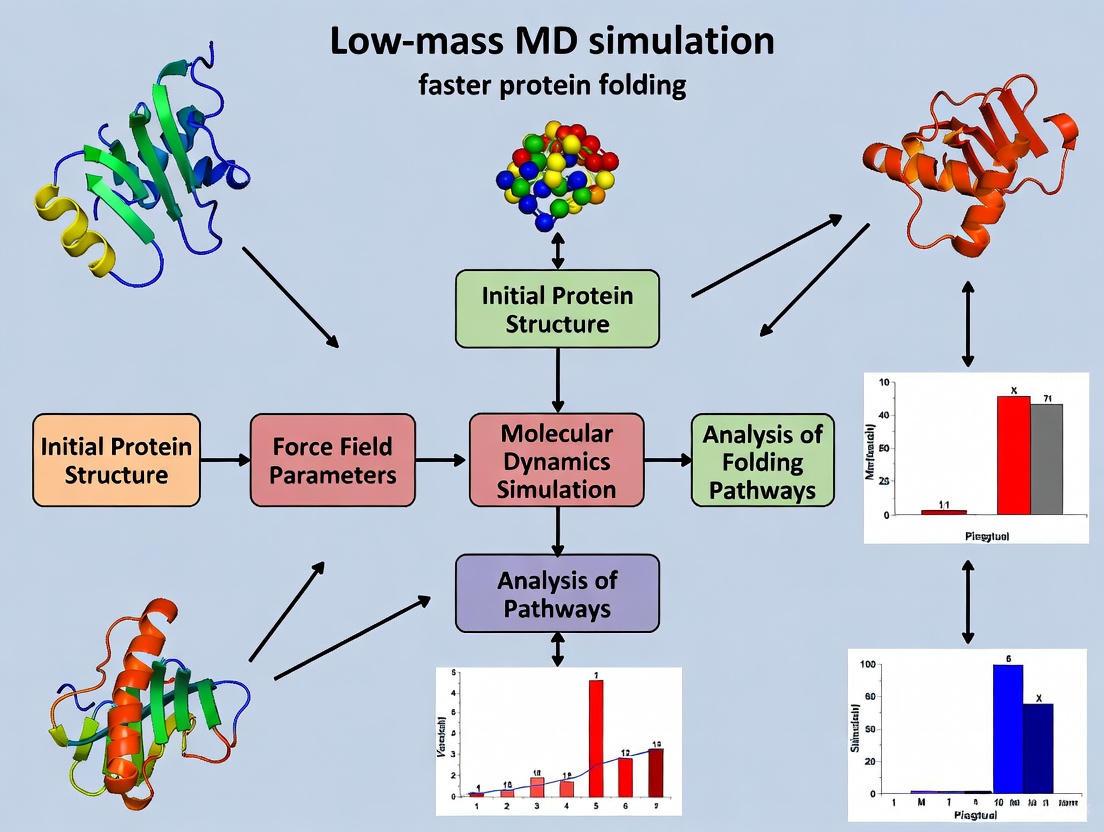
Workflow Visualization
The following diagram illustrates the logical relationship and workflow for implementing the low-mass MD technique, from the core theory to the final analysis.
The Scientist's Toolkit
Essential Software and Parameters
Table 3: Key Configuration Parameters for Low-Mass MD
| Parameter / Component | Recommended Setting | Function and Rationale |
|---|---|---|
| Integrator | Leap-frog (md) or Velocity Verlet (md-vv) |
Standard Newtonian mechanics integrators. [8] |
Time Step (dt) |
1.00 fs | Must be used with low masses to maintain stability and integration accuracy. [2] |
| Mass Scaling | 0.1 (applied to all atoms) | The core parameter that uniformly reduces atomic masses by tenfold. [2] [1] |
| Constraints | SHAKE on all bonds involving H | Allows for the use of a 1 fs time step without bond vibration limitations. [2] |
| Precision | Double-precision | Mandatory to handle the reduced numerical stability of the scaled system. [2] [7] |
| Temperature Control | Berendsen, Nosé-Hoover, etc. | Standard thermostats at T ≤ 340 K. [2] |
| Pressure Control | Isotropic molecule-based scaling | Standard barostat for NPT ensemble. [2] |
| Electrostatics | Particle Mesh Ewald (PME) | Accurate handling of long-range interactions. [2] |
Relationship to Other Sampling Methods
It is important to distinguish low-mass MD from other mass-repartitioning techniques. While low-mass MD applies a uniform mass reduction to all atoms in the system (solute and solvent), methods like hydrogen mass repartitioning (HMR) increase the mass of hydrogen atoms specifically to allow for a larger time step, typically leaving other masses unchanged [8]. The GROMACS mass-repartition-factor parameter, for instance, is an implementation of HMR, not uniform scaling. Low-mass MD is a simpler, more generic technique that does not require differential scaling of atom types, making it straightforward to implement in most MD packages that allow user-defined atomic masses [1].
Molecular dynamics (MD) simulation is a powerful computational technique that provides atomic-level insight into biomolecular processes, including the fundamental problem of protein folding. However, a significant challenge limits its application: the sampling problem. This refers to the inability of standard MD simulations to adequately explore the vast conformational space of a protein within a feasible computational time frame. While major advances have been made in simulating small, fast-folding proteins, research on larger, multidomain proteins—which constitute the majority of proteins—is less advanced due to their complex energy landscapes and long-lived folding intermediates [9].
The core of the issue is timescale disparity. Protein folding in nature can occur on timescales ranging from microseconds to minutes, whereas classical, all-atom MD simulations are often limited to nanoseconds or microseconds, even on specialized supercomputers [9]. This review examines the intrinsic limitations of traditional MD and presents enhanced sampling techniques, with a specific focus on the low-mass MD simulation protocol, as solutions to overcome the sampling problem and propel folding research forward.
The Root of the Problem: Rugged Energy Landscapes and Computational Cost
The sampling problem originates from the complex, multidimensional energy landscape of proteins. According to the principle of minimal frustration, naturally occurring proteins have evolved to have "funneled" energy landscapes that guide them toward the native state. Nevertheless, this landscape remains rugged, featuring numerous local minima and free energy barriers that can trap a simulation [9]. Transitions between these minima are rare events, and for large, slow-folding proteins, even very long simulations are likely to remain confined to a single local minimum, unable to observe a complete folding cycle [9].
The computational expense of MD arises from the need to numerically integrate Newton's equations of motion with a very small time step, typically 1-2 femtoseconds (fs). This fine step is required to accurately capture the fastest vibrations in the system, such as bond stretching involving hydrogen atoms. Consequently, simulating a single microsecond of real-time protein dynamics requires one billion integration steps, making the folding of most proteins prohibitively expensive for all-atom, unbiased MD [10].
Table 1: Key Challenges in Traditional MD Simulations of Protein Folding
| Challenge | Description | Consequence |
|---|---|---|
| Timescale Disparity | Folding occurs from µs to minutes; MD is often limited to ns-µs. | Inability to observe complete folding events. |
| Rugged Energy Landscape | Presence of multiple local minima and high free-energy barriers. | Simulations become trapped in non-native conformations. |
| Small Integration Time Step | Requires 1-2 fs to resolve fast atomic vibrations. | Billions of steps needed for µs-scale simulation; high computational cost. |
| System Size Limitations | Larger proteins and explicit solvent require more atoms. | Increased computational demand per time step. |
Enhanced Sampling Strategies: A Multi-Pronged Approach
To circumvent the sampling problem, numerous enhanced sampling methods have been developed. These can be broadly categorized into methods that bias the simulation to escape energy minima and those that simplify the physical model to accelerate dynamics.
Knowledge-Based and Biased Potential Methods
Structure-based models (SBMs), or Gō models, offer a highly efficient approach by encoding the native structure of the protein directly into the potential energy function, largely ignoring non-native interactions [9]. This simplification creates a perfectly funneled landscape, making folding computationally accessible and allowing for the prediction of folding mechanisms and intermediates. Biased potential techniques, such as umbrella sampling and meta-dynamics, use external potentials to force the system to explore high-energy regions or specific reaction coordinates, thus improving the calculation of free energies [10].
Generalized Ensemble and Replica Exchange Methods
Replica exchange molecular dynamics (REMD), also known as parallel tempering, runs multiple replicas of the system at different temperatures. Periodically, exchanges between replicas are attempted based on a Metropolis criterion. This allows conformations trapped in low-temperature energy minima to escape via high-temperature replicas, leading to a more thorough exploration of the energy landscape [10].
Low-Mass MD: A Simple and Generic Sampling Enhancement Protocol
Low-mass molecular dynamics (LMD) is a simple yet powerful technique that directly addresses the root of the sampling problem—the small integration time step. The protocol is based on a key physical insight: the maximum permissible time step in an MD simulation is limited by the highest vibrational frequency in the system, which is inversely proportional to the square root of the atomic mass. By systematically reducing the masses of hydrogen atoms (or all atoms), the highest frequencies are increased, allowing for a larger integration time step and thus enabling the simulation to cover more real time with fewer computational steps [1] [11].
Quantitative Evidence of Efficacy
The effectiveness of LMD was demonstrated in a landmark study on CLN025, a 10-residue β-hairpin and one of the smallest fast-folding proteins. The results, summarized in Table 2, show a dramatic improvement in sampling efficiency.
Table 2: Performance Comparison: Traditional MD vs. Low-Mass MD for CLN025 Folding
| Parameter | Traditional MD (FF12SB/FF14SB) | Low-Mass MD (10x Mass Reduction) |
|---|---|---|
| Atomic Masses | Standard / Physical | Reduced by 10-fold |
| Number of Simulations | 10 | 10 |
| Simulation Length | 500 ns each | 500 ns each |
| Observed Folding Events | 0 | 4 (out of 10 simulations) |
| Earliest Folding Time | N/A | 66.1 ns |
| Total Sampling | 5 µs | 5 µs |
| Conclusion | Failed to fold | Autonomous and repeated folding achieved |
In this study, the use of AMBER forcefield derivatives with 10-fold reduced atomic masses enabled the autonomous folding of CLN025 from a fully extended conformation to its native structure in explicit solvent at 277 K and 1 atm. In contrast, not a single folding event was observed in simulations of the same length using standard atomic masses [1] [11]. This establishes LMD as a "simple and generic technique to enhance configurational sampling" [11].
Detailed Low-Mass MD Protocol for Protein Folding
This protocol describes the steps to set up and run a low-mass MD simulation to enhance the sampling of protein folding, using the simulation of CLN025 as a benchmark example.
Research Reagent Solutions
Table 3: Essential Materials and Software for Low-Mass MD
| Item | Function/Description |
|---|---|
| Protein System | CLN025 (PDB: 5AWL) or other miniature protein (e.g., Villin Headpiece, WW domain). |
| MD Simulation Engine | Software like AMBER, GROMACS, NAMD, or DESMOND. The protocol is software-agnostic. |
| All-Atom Force Field | AMBER FF12SB/FF14SB derivatives or equivalents (e.g., CHARMM, OPLS-AA). |
| Explicit Solvent Model | TIP3P, SPC/E, or other water models compatible with the chosen force field. |
| Neutralizing Ions | Na⁺, Cl⁻ or other ions to achieve system electroneutrality. |
| Energy Minimization Tool | Integrated tool within the chosen MD engine (e.g., sander in AMBER, grompp in GROMACS). |
| Equilibration & Production Scripts | Custom scripts to run the simulation stages (minimization, equilibration, production). |
Step-by-Step Procedure
System Preparation:
- Obtain the initial coordinates for the protein, typically in a fully extended backbone conformation for de novo folding studies.
- Place the protein in a suitably sized simulation box (e.g., a rectangular or dodecahedron box) with a buffer of explicit solvent molecules (e.g., 1.0 nm from the protein to the box edge).
- Add ions to neutralize the system's net charge and, optionally, to achieve a physiological salt concentration.
Mass Rescaling:
- This is the critical step. Modify the force field parameter files or the system topology to reduce the masses of all atoms by a uniform factor. A 10-fold mass reduction has been successfully demonstrated [1] [11].
- Note: The charges, bond lengths, and angles remain unchanged. Only the masses are altered.
Energy Minimization:
- Perform energy minimization of the solvated and ionized system to remove any bad steric contacts and relax the structure.
- Typical method: Steepest descent algorithm for 1,000-5,000 steps.
System Equilibration:
- Equilibrate the system in two phases:
- NVT Ensemble: Heat the system from 0 K to the target temperature (e.g., 277 K) over 100 ps, using a weak coupling thermostat (e.g., Berendsen or Nosé-Hoover). Restrain the heavy atom positions of the protein.
- NPT Ensemble: Equilibrate the system at the target temperature and pressure (1 atm) for 100-500 ps, using a weak coupling barostat (e.g., Berendsen or Parrinello-Rahman). Maintain positional restraints on protein heavy atoms.
- Equilibrate the system in two phases:
Production Simulation:
- Run the production MD simulation in the NPT ensemble without any positional restraints.
- Use the target temperature and pressure (277 K, 1 atm in the benchmark study).
- Apply a time step of 2-4 femtoseconds. The increased time step is valid due to the reduced atomic masses.
- Run multiple independent simulations (e.g., 10x 500 ns) to ensure statistical significance and to observe rare events like folding.
Trajectory Analysis:
- Monitor folding using root mean square deviation (RMSD) of the protein backbone relative to the known native structure.
- Calculate the radius of gyration (Rg) to track compaction.
- Use native contact analysis (Q) to quantify the formation of correct tertiary contacts.
Visualization of the Low-Mass MD Protocol and Folding Landscape
The following diagram illustrates the logical workflow of the Low-Mass MD protocol and its impact on the protein folding energy landscape.
The sampling problem presents a formidable barrier to studying protein folding using traditional MD simulations. While advanced hardware and specialized supercomputers offer one path forward, enhanced sampling algorithms provide a more accessible and universally applicable solution. Among these, the low-mass MD technique stands out for its simplicity and demonstrated efficacy. By enabling larger integration time steps through a reduction in atomic masses, LMD directly accelerates the exploration of conformational space. As evidenced by the successful folding of CLN025, this generic technique can make the autonomous folding of miniature proteins practical on commodity computers, representing an important step forward for computational quantitative biology and drug development [1] [11].
The process by which a protein folds from a linear amino acid chain into a precise three-dimensional structure is fundamental to biology. Molecular dynamics (MD) simulation has long promised to provide an atomistic-resolution view of this process, but for years, computational limitations made it impossible to observe small proteins folding autonomously in simulations without experimental data guiding the process. The 10-residue miniprotein CLN025, a designed beta-hairpin, became an important model system in this quest due to its small size and fast experimental folding time [12]. A key historical barrier was broken when researchers achieved the first autonomous folding of CLN025 from a fully extended conformation to its native structure in classical, all-atom, isothermal-isobaric MD simulation. This breakthrough was accomplished not by increasing computational power, but by implementing an innovative low-mass molecular dynamics (LMD) simulation technique, which dramatically enhanced configurational sampling and made folding simulations feasible on commodity hardware [1] [13].
Breakthrough Methodology: Low-Mass Molecular Dynamics
The core innovation that enabled this milestone was a simple yet powerful modification to the physical parameters of the simulation: reducing the mass of all atoms by a factor of ten.
Theoretical Basis of the Low-Mass Technique
In molecular dynamics, the maximum permissible integration time step is limited by the highest frequency vibrations in the system, which are typically bond stretches involving hydrogen atoms. Reducing atomic masses increases the frequency of these vibrations. Counter-intuitively, the LMD technique capitalizes on this by using a mass of 0.1 atomic mass units (amu) for all atoms, which allows for a larger integration time step without sacrificing simulation stability. This approach vastly improves sampling efficiency within a given simulation wall-clock time, effectively accelerating the observation of rare events like folding transitions [1].
Experimental Protocol: Implementing LMD for CLN025 Folding
The following detailed protocol recreates the methodology that first achieved CLN025's autonomous folding:
Step 1: System Preparation
- Obtain the fully extended backbone conformation of CLN025 (10 residues).
- Solvate the protein in an explicit solvent box (e.g., TIP3P water model) with appropriate ion concentration to neutralize the system charge.
- Ensure the system is under isothermal-isobaric (NPT) ensemble conditions (1 atm, 277 K) to mimic the experimental folding environment [1].
Step 2: Forcefield and Parameter Modification
Step 3: Simulation Execution
- Perform multiple, independent MD simulations (e.g., 10x 500-ns runs) on standard computing hardware (the original study used Apple Mac Pros).
- Use a Langevin dynamics integrator to control temperature and a Berendsen barostat for pressure regulation.
- Monitor the Cα and Cβ root mean square deviation (CαβRMSD) relative to the known native structure (PDB: 2RVD) to track folding events [1].
Step 4: Analysis and Validation
- A successful folding event is identified when the CαβRMSD to the native conformation falls and remains below a defined threshold (typically ~1 Å).
- Confirm the folded structure by checking for the characteristic beta-hairpin geometry and key stabilizing hydrogen bonds between residues such as Tyr1 and Trp2 [12].
- Compare the simulated folding time (time to first folding event) with experimental values for validation.
Diagram 1: The Low-Mass MD Simulation Workflow for CLN025 Folding.
Key Experimental Results and Performance Data
The application of the LMD technique yielded definitive and reproducible folding of CLN025, a feat not previously achieved with standard MD parameters.
Quantitative Folding Results
The table below summarizes the key quantitative outcomes from the landmark LMD folding experiment.
Table 1: Key Experimental Results from the First Autonomous Folding of CLN025 using LMD
| Parameter | Result with Low-Mass MD | Result with Standard Mass MD | Experimental Reference |
|---|---|---|---|
| Simulation Technique | Low-Mass (0.1 amu) | Standard Atomic Masses | N/A |
| Folding Observed? | Yes, in 4 out of 10 simulations | No folding observed in 10 simulations | N/A |
| First Folding Time | As early as 66.1 ns | Not Applicable | Varies with temperature |
| Folding Temperature | 277 K (Simulation condition) | 277 K (Simulation condition) | ~340 K (Melting point) [12] |
| Critical Technique | 10-fold atomic mass reduction | Standard AMBER forcefields | N/A |
Benchmarking Against Later Simulations
Subsequent methodological improvements eventually achieved agreement with experimental folding times using different approaches. The following table places the initial LMD breakthrough in the context of later successes.
Table 2: Evolution of Simulated vs. Experimental Folding Times for CLN025
| Simulation Study & Conditions | Temperature | Simulated Folding Time (τ) | Experimental Folding Time (τ) | Agreement Factor (Sim/Exp) |
|---|---|---|---|---|
| Early Microcanonical (NVE) MD [14] | 300 K | > 4-10x longer than experiment | 0.137 μs | > 4.0 |
| Isobaric-Isothermal (NTP) MD [14] [5] | 293 K | 0.279 μs | 0.261 μs | 1.07 |
| Isobaric-Isothermal (NTP) MD [14] [5] | 300 K | 0.198 μs | 0.137 μs | 1.45 |
| Low-Mass MD (LMD) [1] | 277 K | 66.1 ns (first event) | Not explicitly stated for 277K | Qualitative folding achieved |
The Scientist's Toolkit: Essential Research Reagents and Solutions
This table details the key computational "reagents" required to implement the low-mass MD technique for protein folding studies.
Table 3: Essential Research Reagent Solutions for Low-Mass MD Simulations
| Item Name | Function / Role in the Experiment | Specification / Notes |
|---|---|---|
| CLN025 Miniprotein | Model fast-folding system | 10-residue beta-hairpin (PDB ID: 2RVD) [12] |
| AMBER Forcefield | Defines interatomic potentials | FF12SB or FF14SB derivatives; parameters must be modified for low mass [1] [13] |
| Low-Mass Parameters | Enables enhanced configurational sampling | Modified forcefield with all atomic masses set to 0.1 atomic mass units (amu) [1] |
| Explicit Solvent Model | Provides realistic solvation environment | Typically the TIP3P water model is used [1] |
| MD Simulation Engine | Executes the numerical integration of equations of motion | Software supporting parameter modification (e.g., AMBER, GROMACS, CHARMM, or OPENMM) |
| CαβRMSD Metric | Primary reaction coordinate for tracking folding | Measurement of Cα and Cβ root mean square deviation from native structure [1] |
The successful autonomous folding of CLN025 using low-mass MD simulation represented a pivotal moment in computational biophysics. It demonstrated that classical, all-atom folding simulations on commodity computers were achievable for fast-folding proteins, a crucial step forward in quantitative biology [1]. While later studies refined techniques to match experimental folding rates more accurately in different thermodynamic ensembles [14] [5], the LMD technique proved itself as a simple, generic, and powerful method for enhancing configurational sampling. This breakthrough opened new prospects for developing algorithms that can predict not only protein structure but also the kinetics of folding, ultimately contributing to a deeper understanding of how protein dynamics govern cellular function.
Implementing Low-Mass MD: A Step-by-Step Protocol for Protein Folding
The reliability of a molecular dynamics (MD) simulation is fundamentally determined by the quality of the initial system setup. A properly prepared protein-solvent environment minimizes instabilities, ensures realistic thermodynamic behavior, and is a critical prerequisite for obtaining scientifically valid results. For advanced sampling techniques like low-mass MD (LMD), which enhances conformational sampling by reducing atomic masses to accelerate dynamics, a stable initial configuration is even more crucial to prevent numerical instabilities and maximize the technique's benefit [11] [1]. This application note provides detailed, step-by-step protocols for preparing a robust protein-solvent system, with a specific focus on its role within a research thesis investigating LMD for faster protein folding.
A Ten-Step Protocol for Stable System Preparation
A comprehensive, ten-step protocol is recommended to gradually relax the system and avoid large initial forces that can cause simulation failures [15]. The procedure involves a series of energy minimizations and short molecular dynamics simulations with progressively weakening positional restraints. An overview of the complete workflow is provided in Figure 1.
Figure 1. System Preparation Workflow. This diagram outlines the sequential steps for preparing a stable simulation system, moving from initial minimization of solvent and ions to full equilibration.
The following is the detailed protocol. Note that all positional restraints are applied to the heavy (non-hydrogen) atoms of the large molecules (proteins, nucleic acids) using the initial coordinates as a reference [15].
Step 1: Initial minimization of mobile molecules
- Action: 1,000 steps of Steepest Descent (SD) minimization.
- Restraints: Strong positional restraints (force constant of 5.0 kcal/mol·Å²).
- Constraints: No constraints (e.g., SHAKE) should be applied.
Step 2: Initial relaxation of mobile molecules
- Action: 15 ps of MD simulation in the NVT ensemble with a 1 fs timestep.
- Restraints: Strong positional restraints (5.0 kcal/mol·Å²).
- Constraints: Apply constraints (e.g., SHAKE) for bonds involving hydrogen.
- Thermostat: Weak-coupling thermostat with a time constant of 0.5 ps.
Step 3: Initial minimization of large molecules
- Action: 1,000 steps of SD minimization.
- Restraints: Medium positional restraints (force constant of 2.0 kcal/mol·Å²).
Step 4: Continued minimization of large molecules
- Action: 1,000 steps of SD minimization.
- Restraints: Weak positional restraints (force constant of 0.1 kcal/mol·Å²).
Step 5: Final minimization of the entire system
- Action: 1,000 steps of SD minimization.
- Restraints: No positional restraints.
Step 6: Relaxation of substituents
- Action: 5 ps of MD simulation in the NVT ensemble with a 1 fs timestep.
- Restraints: Positional restraints on the backbone heavy atoms only.
- Constraints: Apply constraints for bonds involving hydrogen.
Step 7: Relaxation of the entire system
- Action: 5 ps of MD simulation in the NVT ensemble with a 1 fs timestep.
- Restraints: No positional restraints.
- Constraints: Apply constraints for bonds involving hydrogen.
Step 8: Relaxation of substituents at constant pressure
- Action: 5 ps of MD simulation in the NPT ensemble with a 1 fs timestep.
- Restraints: Positional restraints on the backbone heavy atoms only.
- Constraints: Apply constraints for bonds involving hydrogen.
- Barostat: Weak-coupling barostat.
Step 9: Relaxation of the entire system at constant pressure
- Action: 5 ps of MD simulation in the NPT ensemble with a 1 fs timestep.
- Restraints: No positional restraints.
- Constraints: Apply constraints for bonds involving hydrogen.
- Barostat: Weak-coupling barostat.
Step 10: System equilibration
- Action: MD simulation in the NPT ensemble until the system density stabilizes.
- Criteria: The simulation is continued until the density reaches a plateau, which can be tested by checking that the slope of the density vs. time plot approaches zero over a suitable window [15].
- Restraints & Constraints: No positional restraints; bond constraints applied.
Implementing the Low-Mass MD Technique
Once a conventional system is fully equilibrated using the protocol above, the LMD simulation can be initiated. This technique is a simple yet powerful way to enhance conformational sampling.
- Core Principle: LMD enhances configurational sampling by reducing the atomic masses in the system, which allows for faster dynamics and more rapid exploration of conformational space [11] [1].
- Methodology: A 10-fold reduction of all atomic masses is a typical and effective approach. For example, in studies of the fast-folding protein CLN025, this reduction enabled autonomous folding in simulations on the hundred-nanosecond timescale, a feat not achieved with standard masses [11].
- Implementation Workflow: The logical relationship and key parameter for implementing LMD are summarized in Figure 2.
Figure 2. Low-Mass MD Implementation. This diagram shows the process of initiating a low-mass MD simulation from an equilibrated system to achieve enhanced sampling.
Research Reagent and Tool Kit
A successful simulation requires a suite of software tools and carefully prepared inputs. The table below details the essential components for setting up and running a simulation, particularly using the GROMACS suite [16] [17].
Table 1: Essential Research Reagents and Tools for MD System Setup
| Item Name | Function/Description | Example/Note |
|---|---|---|
| Protein Structure File | Initial atomic coordinates. | PDB format file from RCSB PDB or homology modeling [16]. |
| Molecular Topology File | Describes the molecule(s), including bonds, angles, force field parameters, and charges. | GROMACS .top file, generated by pdb2gmx or tools like CHARMM-GUI [16] [18]. |
| Molecular Geometry File | Contains the system's coordinates, velocities, and box dimensions. | GROMACS .gro file [16]. |
| Force Field | Defines the functional form and parameters for potential energy calculations. | AMBER (e.g., FF14SB), CHARMM, GROMOS. Choice depends on the system [11] [17]. |
| Simulation Parameter File | Specifies all control parameters for the simulation steps. | GROMACS .mdp file for minimization, equilibration, and production [16]. |
| Solvent Model | Represents water molecules in the explicit solvent. | TIP3P, SPC/E. Must be consistent with the chosen force field [17]. |
| Ions | Neutralize the system's net charge and mimic physiological ionic strength. | Sodium (Na⁺), Chloride (Cl⁻) ions [16]. |
| Simulation Software | The MD engine used to run the simulations. | GROMACS, NAMD, AMBER, OpenMM [15] [17] [18]. |
| Visualization Software | Used to inspect structures and trajectories. | RasMol, VMD, PyMOL [16]. |
Quantitative Data for Low-Mass MD Simulations
The effectiveness of the LMD technique is demonstrated by quantitative comparisons with standard MD simulations. The following table summarizes key performance metrics from a study on the CLN025 protein [11] [1].
Table 2: Performance Comparison: Standard MD vs. Low-Mass MD
| Parameter | Standard MD (FF12SB/FF14SB) | Low-Mass MD (10x Reduced Mass) |
|---|---|---|
| Number of Folding Events | 0 out of 10 simulations | 4 out of 10 simulations |
| Time to First Fold | Not Observed (N/A) | As early as 66.1 ns |
| Simulation Length | 10 x 500 ns | 10 x 500 ns |
| Sampling Efficiency | Limited, no native state reached | Vastly improved, repeated folding/unfolding |
| Hardware Used | Apple Mac Pros | Apple Mac Pros |
This data clearly shows that the LMD technique can successfully drive protein folding in simulations that are otherwise too short to observe the phenomenon, making it a powerful tool for folding research on commodity hardware [11].
Molecular dynamics (MD) simulation is a powerful technique for studying protein folding at atomic resolution, but its effectiveness is often hampered by the limited timescales accessible to conventional computational resources [4]. The configurational sampling necessary to observe folding events requires sophisticated parameter configuration to enhance simulation efficiency without sacrificing physical accuracy. This application note details key parameter configurations—specifically mass scaling, time step selection, and temperature control—that can significantly accelerate protein folding simulations. These techniques are framed within the context of low-mass MD simulation methodology, a promising approach for achieving faster convergence to native protein structures, which is of critical importance to researchers and drug development professionals seeking to understand protein function and stability.
Quantitative Data Comparison
Mass Scaling and Time Step Parameters
Table 1: Comparative sampling efficiencies of mass and time step configurations
| Mass Scaling Factor (λ) | Time Step (fssmt) | Theoretical Time Scaling | Relative Sampling Efficiency | Optimal Temperature Range | Key Advantages |
|---|---|---|---|---|---|
| 0.1 (Low-mass) | 1.00 | √10 [2] | Better than std mass Δt=2.00 fssmt [2] | ≤ 340 K [2] | Enhanced sampling without SHAKE failure; simple implementation |
| 1.0 (Standard) | 2.00 | 1 | Baseline (Routine) [2] | ≤ 300 K [2] | Standard approach; well-characterized |
| 1.0 (Standard) | 3.16 | √10 [2] | Equal to low-mass Δt=1.00 fssmt [2] | ≤ 340 K [2] | Equivalent sampling to low-mass method; fewer steps needed |
| 1.0 (Standard) | 3.50 | - | Potential instability [2] | - | High risk of SHAKE failure [2] |
Temperature-Dependent Performance
Table 2: Temperature effects on simulation methods and sampling
| Simulation Method | Temperature Conditions | Observed Performance and Applications |
|---|---|---|
| Low-mass NTP MD [2] | 277 K, 300 K, 340 K | Reliable folding of β-hairpins (chignolin, CLN025); robust sampling across temperatures |
| Standard-mass NTP MD [2] | 277 K, 300 K, 340 K | Successful at routine Δt=2.00 fssmt; instability risk at Δt≥3.16 fssmt without mass repartitioning |
| Accelerated MD (AMD) [19] | 300 K, 350 K, 400 K, 450 K | Successful helical protein folding at 300K in 40-180 ns; higher temperatures increase sampling but 300K most suitable for correct folding |
| Deep Learning (aSAMt) [20] | 320 K to 450 K | High-temperature training enhances exploration of energy landscapes; generalizes to unseen temperatures |
Experimental Protocols
Low-Mass MD Simulation for Enhanced Sampling
This protocol describes the procedure for setting up and running low-mass molecular dynamics simulations to enhance configurational sampling in protein folding studies, based on methodologies that have successfully folded β-hairpin systems like chignolin and CLN025 [2].
System Preparation
- Initial Structure Generation: Create a fully extended backbone conformation (anti-parallel β-strand) of the target protein using molecular visualization software such as PyMOL [2].
- Solvation and Neutralization: Solvate the protein in TIP3P water model within a periodic boundary box. Add counterions to neutralize system charge and NaCl molecules to achieve physiological ionic concentration [2].
- Energy Minimization: Perform 100 cycles of steepest-descent minimization followed by 900 cycles of conjugate-gradient minimization to remove close van der Waals contacts [2].
Simulation Parameters
- Mass Scaling: Uniformly reduce all atomic masses by a factor of ten (λ=0.1) [2].
- Time Step: Use a time step of 1.00 fssmt (femtoseconds of standard-mass time) [2].
- Temperature Coupling: Employ the Berendsen coupling algorithm with constant temperature (NTP MD) at biologically relevant temperatures (≤340 K) [2].
- Pressure Coupling: Use isotropic molecule-based scaling at 1 atm pressure [2].
- Bond Constraints: Apply the SHAKE algorithm to constrain all bonds involving hydrogen atoms [2].
- Electrostatics: Calculate long-range electrostatic interactions using the Particle Mesh Ewald method [2].
- Non-bonded Interactions: Set a cutoff of 8.0 Å for nonbonded interactions [2].
Simulation Execution
- Heating Phase: Heat the system from 0 to the target temperature (277, 300, or 340 K) at a rate of 10 K/ps under constant volume conditions [2].
- Production Run: Perform production simulation under constant temperature and pressure (NTP) for sufficient time steps (e.g., 500×10⁶ steps) to observe folding events [2].
- Replication: Conduct multiple independent simulations (e.g., 20 replicates) with different initial velocity distributions to ensure statistical significance [2].
Data Analysis
- Folding Assessment: Monitor folding progress using Cα and Cβ root mean square deviation (CαβRMSD) from native structures determined experimentally (e.g., by NMR) [2].
- Sampling Efficiency: Compare the number of time steps required to capture folding events against standard-mass simulations [2].
- Native Contacts: Track formation of native contacts throughout the simulation trajectory [2].
Temperature-Conditioned Deep Learning for Ensemble Generation
This protocol outlines the use of deep generative models trained on MD simulation data to generate temperature-dependent structural ensembles of proteins, providing a computationally efficient alternative to long MD simulations [20].
Model Architecture Setup
- Model Selection: Implement aSAMt (atomistic Structural Autoencoder Model temperature-conditioned), a latent diffusion model designed for generating heavy atom protein ensembles conditioned on temperature [20].
- Autoencoder Component: Train an autoencoder to represent heavy atom coordinates of proteins as SE(3)-invariant encodings [20].
- Diffusion Component: Train a diffusion model to learn the probability distribution of encodings, conditioned on both an initial 3D structure and temperature [20].
Training Procedure
- Dataset Preparation: Utilize the mdCATH dataset, which contains MD simulations for thousands of globular protein domains at different temperatures (320-450 K) [20].
- Model Training: Train the aSAMt model on multiple proteins across various temperatures to enable generalization to unseen sequences and temperatures [20].
- Validation: Assess decoder performance by reconstructing encoded conformations; target heavy atom RMSD of 0.3-0.4 Å from MD snapshots [20].
Ensemble Generation
- Sampling: Generate ensembles by sampling encodings via the diffusion model and decoding them to 3D structures [20].
- Energy Minimization: Apply a brief energy minimization protocol to generated structures to resolve atom clashes while restraining backbone atoms to 0.15-0.60 Å RMSD [20].
- Temperature Conditioning: Input desired temperature values to generate ensembles specific to thermodynamic conditions of interest [20].
Validation and Analysis
- Local Flexibility: Calculate Cα root mean square fluctuation (RMSF) profiles and compare to reference MD simulations using Pearson correlation coefficient [20].
- Torsion Angles: Evaluate backbone (φ/ψ) and side chain (χ) torsion angle distributions using WASCO scores [20].
- Landscape Coverage: Use principal component analysis (PCA) to assess coverage of conformational space compared to reference MD ensembles [20].
Signaling Pathways and Workflows
The Scientist's Toolkit
Table 3: Essential research reagents and computational tools for low-mass MD protein folding studies
| Tool/Resource | Type | Primary Function | Application Notes |
|---|---|---|---|
| AMBER MD Package [2] | Software Suite | Molecular dynamics simulation | Includes SANDER for minimization; PMEMD for production MD; supports mass scaling parameters |
| SHAKE Algorithm [2] | Computational Method | Bond-length constraints | Essential for constraining bonds involving H; enables longer time steps |
| TIP3P Water Model [2] | Solvation Model | Explicit solvent representation | Used for solvating protein systems; affects viscosity and sampling |
| Charmm22/FF14SB [2] [21] | Force Field | Potential energy parameters | FF14SB: general-purpose; Charmm22: used in folding energetics studies |
| aSAMt [20] | Deep Learning Model | Temperature-conditioned ensemble generation | Generates structural ensembles at specified temperatures; trained on MD data |
| BioEmu [22] | Biomolecular Emulator | Sampling equilibrium conformations | Uses diffusion model for rapid structure generation (minutes to hours on GPU) |
| mdCATH Dataset [20] | Training Data | MD simulations of protein domains | Contains simulations at multiple temperatures (320-450K) for training generative models |
| ATLAS Dataset [20] | Training Data | MD simulations of protein chains | Used for training constant-temperature ensemble generators |
The AMBER (Assisted Model Building with Energy Refinement) force field family is a cornerstone for molecular dynamics (MD) simulations of proteins and nucleic acids. Among its derivatives, ff14SB is a highly refined, all-atom force field designed to accurately model protein dynamics. Its development was driven by identified weaknesses in its widely-used predecessor, ff99SB, particularly concerning side chain rotamer preferences and backbone secondary structure propensities [23]. The ff14SB force field incorporates two major improvements: a complete refit of all amino acid side chain dihedral parameters based on multidimensional quantum mechanical (QM) scans, and an empirical adjustment to the protein backbone dihedral parameters, specifically in the φ rotational profile [23]. These changes resulted in a 35% reduction in average errors for relative energies of conformation pairs compared to QM calculations and improved reproduction of NMR scalar coupling data and secondary structure content in peptides [23].
The ff12SB parameter set is a preliminary version of ff14SB that includes most of its core improvements [23]. It serves as a direct evolutionary step between ff99SB and the more refined ff14SB. When discussing compatibility and performance, ff12SB and ff14SB are often grouped closely together, with ff14SB representing the more finalized and recommended version for most modern protein simulations [23] [24]. The primary strength of these force fields lies in their balanced accuracy for simulating a wide range of protein properties, including stable secondary structure content, realistic side chain dynamics, and correct local backbone dynamics as measured by NMR order parameters [23].
Performance and Compatibility in Standard MD Simulations
The ff14SB force field is parameterized for use with explicit solvent models, such as TIP3P, and is the recommended choice for protein simulations within the AMBER ecosystem [23] [24]. Its compatibility is designed to be broad, allowing researchers to generate simulation input files seamlessly using the Amber leap program [24].
Quantitative benchmarks demonstrate that ff14SB offers significant improvements over previous force fields. The following table summarizes key performance metrics for ff14SB compared to its predecessor, ff99SB:
Table 1: Quantitative Performance Comparison of ff14SB vs. ff99SB
| Performance Metric | ff99SB | ff14SB | Improvement/Benchmark |
|---|---|---|---|
| Avg. Relative Energy Error (vs. QM) | ~1.54 kcal/mol | <1.0 kcal/mol | 35% reduction [23] |
| NMR χ1 Scalar Couplings | Less accurate | Better reproduction | Improved agreement with experimental data for proteins in solution [23] |
| Secondary Structure Content | Exaggerated helical propensity in ff94/99; improved balance in ff99SB | Further improved balance | Better reproduction in small peptides [23] |
| Protein Crystallography | Good | Superior | Better maintenance of crystal lattice and protein conformations for triclinic lysozyme vs. ff99SB and CHARMM36 [23] |
Beyond these specific metrics, ff14SB has been shown to maintain protein conformations in crystal lattices more effectively than several other contemporary force fields, including CHARMM36 [23]. It is important to note that the performance of a force field can be significantly influenced by the chosen water model. Studies have indicated that the standard TIP3P water model, while compatible, can sometimes lead to artificial structural collapse in disordered protein regions. Alternative models like TIP4P-D have been shown to improve reliability in simulations containing intrinsically disordered regions when combined with biomolecular force fields like ff14SB [25].
Application in Low-Mass MD Simulations for Protein Folding
Low-mass molecular dynamics (LMD) is a simple and generic sampling enhancement technique where all atomic masses are uniformly reduced, typically by tenfold. This method can vastly improve configurational sampling, enabling phenomena like protein folding to be observed on significantly shorter simulation timescales [1] [2].
The ff12SB and ff14SB force fields are fully compatible with the LMD technique. Research has directly employed these force fields in LMD simulations to study the folding of mini-proteins. The core theory behind LMD states that scaling the total mass of a system by a factor of λ (e.g., 0.1) scales the time of the new system by a factor of √λ. This makes a low-mass simulation at a time step of 1.00 fs of the standard-mass time (fssmt) theoretically equivalent to a standard-mass simulation at a time step of √10 ≈ 3.16 fssmt [2]. This equivalence allows for more configuration space to be explored per unit of computational time.
Table 2: Low-Mass MD Performance with AMBER Force Fields
| Simulation Condition | Folding Outcome (CLN025) | Sampling Efficiency | Key Findings |
|---|---|---|---|
| Standard Mass (FF12SB/FF14SB)Δt=2.00 fssmt | No folding observed in ten 500-ns simulations [1] | Baseline | Standard masses with routine time step were insufficient to observe folding in these runs. |
| Low Mass (FF12SB/FF14SB)Δt=1.00 fssmt | Autonomous folding in 4 of 10 simulations; first fold at 66.1 ns [1] | Statistically better than standard mass at Δt=2.00 fssmt [2] | Mass reduction enables folding on commodity hardware by enhancing sampling. |
| Standard Mass at Δt=3.16 fssmt | Not specifically reported for CLN025 | Statistically equivalent to low-mass at Δt=1.00 fssmt [2] | Confirms theoretical equivalence; however, such long time steps are often numerically unstable with standard integrators. |
LMD provides a practical pathway to accelerate folding research. For instance, the β-hairpin protein CLN025, one of the smallest fast-folding proteins, folded autonomously from a fully extended conformation to its native state in explicit solvent in multiple 500-ns LMD simulations using AMBER force field derivatives, with the first folding event occurring as early as 66.1 ns. By contrast, no folding was observed when the simulations were repeated using the original AMBER ff12SB and ff14SB force fields with standard atomic masses [1]. This highlights LMD as a powerful complementary technique to force fields like ff14SB for studying protein folding.
The diagram below illustrates the workflow for selecting and applying AMBER force fields in conjunction with the low-mass MD technique for protein folding studies.
Essential Research Reagents and Computational Tools
Successful implementation of MD simulations using ff12SB/ff14SB and the LMD technique requires a suite of well-defined research reagents and software tools. The table below details the essential components for setting up and running these experiments.
Table 3: Research Reagent Solutions for AMBER MD Simulations
| Item Name | Function / Role | Example / Specification |
|---|---|---|
| AMBER ff14SB Force Field | Provides mathematical functions and parameters for protein energetics and dynamics. | All-atom force field; includes dihedral adjustments for backbone (φ) and side chains [23]. |
| Explicit Solvent Model | Mimics the aqueous environment of biological molecules. | TIP3P (standard) [24]; TIP4P-D (recommended for systems with disordered regions) [25]. |
| Simulation Software | Software suite used to perform energy minimization, heating, equilibration, and production MD. | AMBER (e.g., PMEMD/SANDER) [2]; compatible with other packages like GROMACS and LAMMPS with proper parameter conversion. |
| System Builder | Prepares simulation systems: adds solvent, ions, and generates force field topology files. | tleap/parmed (included in AMBER tools) [24]. |
| Ion Parameters | Models the behavior of counterions and salt concentration in solution. | Revised alkali and halide ion parameters [2]. |
| Visualization & Analysis | Used for visual inspection, trajectory analysis, and result plotting. | VMD, PyMOL, cpptraj (in AMBER), MDTraj. |
| Cluster Model Geometries | Reference data for parameterizing non-standard cofactors (e.g., for cytochrome c oxidase). | XYZ coordinate files derived from density functional theory (DFT) calculations [24]. |
Detailed Experimental Protocol for Low-Mass Folding Simulations
This protocol provides a step-by-step methodology for setting up and running a low-mass MD simulation to study protein folding, using the AMBER ff14SB force field and based on procedures that successfully folded CLN025 [1] [2].
System Preparation and Energy Minimization
- Initial Structure: Obtain or generate a protein structure in a fully extended backbone conformation. Tools like PyMOL can be used for this [2].
- Solvation and Ionization: Solvate the protein in a periodic box of TIP3P water molecules, ensuring a minimum distance (e.g., 8.0 Å) between the protein and box edge. Add counterions to neutralize the system's charge, and optionally add salt to a physiological concentration (e.g., 100 mM NaCl) [2].
- Force Field Assignment: Use the
tleapprogram from the AMBER tools to assign the ff14SB force field parameters to the protein [24]. - Energy Minimization: Perform energy minimization to remove any bad van der Waals contacts. A typical protocol involves:
- 100 cycles of steepest descent minimization.
- Followed by 900 cycles of conjugate gradient minimization [2].
System Equilibration with Standard Masses
- Heating: Heat the system from 0 K to the target temperature (e.g., 277-340 K) over 10-100 ps under constant volume (NVT) or constant pressure (NPT) conditions, using a coupling algorithm like Berendsen [2].
- Equilibration: Run a short equilibration simulation (50-100 ps) with standard atomic masses and a 2.0 fs time step under the desired production conditions (e.g., NPT ensemble at 1 atm and target temperature).
Production Low-Mass MD Simulation
- Mass Modification: Uniformly scale all atomic masses in the system by a factor of 0.1. This can be done by modifying the topology file or using in-built script options in MD software.
- Simulation Parameters:
- Time Step (
Δt): Set to 1.00 fssmt [1] [2]. - Temperature & Pressure: Maintain using a thermostat and barostat (e.g., Berendsen coupling algorithm) [2].
- Bond Constraints: Apply the SHAKE algorithm to constrain all bonds involving hydrogen atoms [2].
- Long-Range Electrostatics: Calculate using the Particle Mesh Ewald (PME) method [2].
- Non-Bonded Cutoff: Set to 8.0 Å [2].
- Time Step (
- Production Run: Launch multiple independent simulations (e.g., 10-20 runs) using different random seeds for initial velocities to ensure statistical robustness. Run each simulation for a sufficient number of steps to observe the folding event (e.g., 500 million steps for a 500-ns simulation) [2].
Data Analysis and Validation
- Folding Trajectory: Monitor the root mean square deviation (CαβRMSD or CRMSD) of the protein structure relative to the known native state to identify folding events [1].
- Equilibrium Properties: Analyze the generated trajectories to compute ensemble properties, such as radius of gyration, secondary structure content, and free energy landscapes.
- Experimental Validation: Where possible, validate simulation results against experimental data, such as NMR chemical shifts, scalar couplings, or known native-state structures [23] [1].
Molecular dynamics (MD) simulation is an indispensable tool for studying protein folding, a fundamental process in quantitative biology and drug discovery. However, capturing the autonomous folding of proteins from an extended conformation in classical, all-atom MD simulations remains computationally challenging due to the timescales involved and the energy barriers between conformational states. The low-mass molecular dynamics (LMD) technique has emerged as a simple, generic, and highly effective method to enhance configurational sampling, enabling the observation of folding events on commodity hardware. This Application Note provides a detailed protocol for implementing LMD simulations to study protein folding, using the fast-folding β-hairpin CLN025 as a model system. The workflow detailed herein is framed within a broader thesis on exploiting mass manipulation to accelerate protein folding research.
Theoretical Basis of Low-Mass MD Simulation
The core principle of the LMD technique is the uniform reduction of atomic masses in the simulated system. Scaling the total mass by a factor of λ (e.g., 0.1 for a 10-fold reduction) effectively scales the time of the new system by a factor of √λ [2]. This relationship arises from the fundamental equations of motion. When the units of distance and energy are kept identical to those of standard-mass simulations, the requirement for consistency in the energy unit, m^2, leads to the relationship [tlmt] = √λ [tsmt], where "lmt" denotes low-mass time and "smt" denotes standard-mass time [2].
Consequently, a simulation using masses reduced by tenfold (λ=0.1) will evolve approximately 3.16 times faster in real time for an equal number of integration steps. In practical terms, an LMD simulation performed with a time step of 1.00 fs of standard-mass time is theoretically equivalent to a standard-mass simulation with a time step of √10 ≈ 3.16 fs [2]. This permits enhanced exploration of conformational space within the same wall-clock time, facilitating the observation of rare events like protein folding.
Materials and Reagents
Research Reagent Solutions
Table 1: Essential materials and software for low-mass MD protein folding simulations.
| Item | Specification / Version | Function / Role in Protocol |
|---|---|---|
| Protein System | CLN025 (10-residue β-hairpin) | A well-characterized, fast-folding miniature protein ideal for method validation [11] [1]. |
| MD Simulation Software | AMBER | MD software package used in the foundational LMD studies; capable of handling modified force field parameters [11] [2]. |
| Force Field | AMBER FF12SB/FF14SB derivatives | The standard force fields, modified to incorporate reduced atomic masses [11] [1]. |
| Solvent Model | TIP3P water model | Explicit solvent model for solvating the protein system [2]. |
| Neutralizing Ions | Revised alkali & halide ion parameters | Sodium and chloride ions to neutralize the system's charge [2]. |
| Commodity Computer Hardware | Apple Mac Pro (or equivalent) | Demonstrates the technique's accessibility; does not require specialized supercomputing resources [11]. |
Experimental Protocol
System Preparation
- Initial Conformation Generation: Generate a fully extended backbone conformation (an anti-parallel β-strand) of the target protein, CLN025. This can be accomplished using molecular visualization software such as PyMOL [2].
- Solvation and Ion Addition: Place the extended conformation in a simulation box and solvate it explicitly with the TIP3P water model. Add a sufficient number of sodium and chloride ions to neutralize the system's net charge and to simulate a physiologically relevant ionic strength (e.g., 150 mM NaCl) [2].
- Force Field Modification: Uniformly reduce the mass of all atoms in the system by a factor of 10 (0.1x) within the AMBER force field parameter files (e.g., derivatives of FF12SB or FF14SB). This is a critical step for enabling the LMD technique [11] [2].
- Energy Minimization: Subject the solvated and ionized system to energy minimization to remove any bad van der Waals contacts. A typical protocol involves 100 cycles of steepest descent followed by 900 cycles of conjugate gradient minimization [2].
Simulation Configuration
- Heating Phase: Heat the minimized system from 0 K to the target simulation temperature (e.g., 277 K, 300 K, or 340 K) over a period of 10-100 ps under constant volume (NVT) or constant pressure (NPT) conditions [2].
- Production Simulation Parameters: Configure the production MD simulation in the NPT ensemble (isothermal-isobaric) at the target temperature (e.g., 277 K) and 1 atm pressure. Key parameters include:
- Time Step: Use a 1.00 fs time step (in standard-mass time units) [11] [2].
- Thermostat/Barostat: Employ the Berendsen coupling algorithm for temperature and pressure control [2].
- Bond Constraints: Apply the SHAKE algorithm to constrain all bonds involving hydrogen atoms [2].
- Long-Range Electrostatics: Calculate using the Particle Mesh Ewald (PME) method [2].
- Non-bonded Cut-off: Set to 8.0 Å [2].
- Periodic Boundary Conditions: Apply in all directions.
- Initial Velocities: Generate initial atomic velocities from a Maxwell-Boltzmann distribution at the target temperature. To ensure statistical independence, run multiple (e.g., 10) replicate simulations, each with a unique random seed for initial velocity assignment [11] [2].
- Simulation Length: Run each simulation for a duration sufficient to capture folding events. For CLN025, 500 ns per replicate is effective, with the first folding events potentially occurring in as little as 66-96 ns [11] [1].
Figure 1: A sequential workflow for setting up and running a low-mass MD simulation to fold a protein from an extended conformation.
Results and Data Analysis
Expected Outcomes and Validation
The primary metric for success is the autonomous folding of the protein from the fully extended state to its native conformation. For CLN025, the native state has been independently determined by NMR spectroscopy and serves as the reference structure [11] [1].
Table 2: Comparative summary of key quantitative results from foundational LMD studies on CLN025 folding [11] [1] [2].
| Simulation Condition | Number of Simulations | Simulation Length | Folding Events Observed | Time to First Fold (ns) |
|---|---|---|---|---|
| Low-Mass (0.1x mass) | 10 | 500 ns | 4 out of 10 | 66.1 - 96.2 |
| Standard Mass (1.0x mass) | 10 | 500 ns | 0 out of 10 | N/A |
Folding should be validated by calculating the root mean square deviation (RMSD) of the simulated structure's carbon atoms (CRMSD) or Cα and Cβ atoms (CαβRMSD) against the known native structure. A successful folding event is characterized by a significant drop in RMSD to a stable, low value (typically < 1-2 Å) that persists for the remainder of the simulation or until unfolding occurs [11] [2].
Comparison with Other Sampling Methods
The efficiency of LMD can be contextualized by comparing it to other common sampling enhancement strategies, such as simply using a longer time step in standard-mass simulations.
Table 3: Comparison of configurational sampling efficiency between LMD and standard-mass MD with extended time steps for folding CLN025 and chignolin [2].
| Simulation Condition | Theoretical Speedup | Effective Sampling vs. Std 2-fs MD | Stability with SHAKE |
|---|---|---|---|
| Low-Mass, 1-fs time step | ~3.16x | Statistically Better | Stable at T ≤ 340 K |
| Standard Mass, 2-fs time step | 1x (Baseline) | Baseline | Stable (Routine) |
| Standard Mass, 3.16-fs time step | ~3.16x | Statistically Equivalent to LMD | Tends to Fail |
Discussion
Technical Advantages and Considerations
The LMD technique offers a straightforward path to enhanced sampling without the complexity of implementing other advanced methods like replica exchange or metadynamics. Its primary advantage is the ability to observe autonomous folding on commodity computers, making this type of research more accessible [11].
A key consideration is the temperature constraint. LMD simulations are typically stable at temperatures of ≤ 340 K. Exceeding this temperature can lead to instabilities due to the higher velocities of the low-mass atoms [2]. Furthermore, while LMD at a 1-fs time step is theoretically equivalent to standard-mass MD at a 3.16-fs time step, the latter often fails in practice with the SHAKE algorithm, which is commonly used for bond constraints. The LMD approach therefore provides a numerically stable route to achieving this level of sampling enhancement [2].
Figure 2: The logical relationship between mass reduction and enhanced sampling, showing how scaling atomic masses leads to faster effective simulation time and improved outcomes.
Application in Drug Discovery
The ability to rapidly simulate folding pathways and generate native conformational ensembles has significant implications in drug discovery. Molecular dynamics simulations are increasingly used to understand the conformational dynamics of drug targets, which is crucial for structure-based drug design [26] [27]. Proteins are dynamic, and ligands often bind to and stabilize specific conformational states [26]. The LMD technique can help generate diverse and physiologically relevant conformational ensembles of miniature proteins or critical protein domains more efficiently, providing a richer structural basis for virtual screening and ligand optimization studies [11] [26]. This can lead to the identification of novel binding pockets and a better understanding of allosteric mechanisms.
The study of protein folding is crucial for understanding biological function and disease mechanisms. Among the various model systems, β-hairpin peptides like CLN025 and chignolin have emerged as fundamental test cases for simulating folding dynamics due to their small size and rapid folding characteristics [28]. This application note details the use of a specific molecular dynamics (MD) technique—low-mass molecular dynamics simulation—to enhance the configurational sampling of these miniature proteins, thereby accelerating folding research [2] [11]. We frame this technique within the broader thesis that strategically reducing atomic masses provides a simple, generic, and computationally efficient path to studying protein folding on commodity hardware, making atomic-detail simulation more accessible to researchers.
Technical Background: Low-Mass MD Simulation
Molecular dynamics simulation is a powerful computational method for studying protein motion at atomic resolution. However, its application is often limited by the small time steps required for numerical stability, which severely restricts the ability to study processes over biologically meaningful timescales [29].
The low-mass MD technique addresses this bottleneck through a simple yet effective modification: uniformly reducing the atomic masses of all atoms in the system by a factor of ten [2] [11]. The theoretical foundation is rooted in classical mechanics. Scaling the total mass of a system by a factor of λ (in this case, 0.1) effectively scales the time of the new system by a factor of √λ [2].
The following diagram illustrates the theoretical equivalence and practical workflow of this approach.
Consequently, a low-mass simulation performed with a time step of 1.00 fs of standard-mass time (fssmt) is theoretically equivalent to a standard-mass simulation with a time step of √10 ≈ 3.16 fssmt [2]. This equivalence allows the low-mass system to effectively sample configuration space more rapidly for the same number of integration steps, significantly enhancing sampling efficiency at temperatures of 340 K and below [2].
Quantitative Comparison of Sampling Techniques
To evaluate the efficacy of low-mass MD simulations, a comparative study was conducted involving 160 unique, independent, all-atom, classical isothermal-isobaric (NTP) MD simulations of the β-hairpins chignolin and CLN025 [2]. The simulations were performed under different conditions to determine relative configurational sampling efficiencies.
Table 1: Comparison of Configurational Sampling Efficiency for CLN025 and Chignolin
| Sampling Technique | Mass Scaling Factor | Time Step (fssmt) | Relative Sampling Efficiency | Key Observations |
|---|---|---|---|---|
| Low-Mass MD | 0.1 | 1.00 | Best | Statistically better than standard mass at 2.00 fssmt; enabled first folding event of CLN025 at 66.1 ns [2] [11]. |
| Standard-Mass MD | 1.0 | 2.00 | Intermediate | Routine time step; no folding event observed with original AMBER forcefields FF12SB/FF14SB [2] [11]. |
| Extended Time-Step MD | 1.0 | 3.16 | Equivalent to Low-Mass | Statistically equivalent to low-mass at 1.00 fssmt, but prone to numerical instability without mass repartitioning [2]. |
| Over-Extended Time-Step MD | 1.0 | 3.50 | Not Reported | SHAKE algorithm tends to fail with time steps ≥ 2.00 fssmt, leading to instability [2]. |
The data confirms that low-mass NTP MD simulations at a time step of 1.00 fssmt provide a simple and generic technique to enhance configurational sampling, offering a practical advantage over the potentially unstable standard-mass simulations at extended time steps [2].
Experimental Protocol: Low-Mass MD Simulation of β-Hairpins
This section provides a detailed, step-by-step protocol for setting up and running low-mass MD simulations to study the folding of β-hairpin peptides like CLN025 and chignolin, based on the methodologies cited in the literature [2] [28].
System Setup and Initialization
- Initial Structure Generation: Generate a fully extended backbone conformation (anti-parallel β-strand) of the target peptide (e.g., CLN025 or chignolin) using molecular visualization software [2].
- Solvation and Ionization: Solvate the peptide in a TIP3P water box. Add counterions to neutralize the system's charge and include NaCl molecules to simulate physiological ionic strength [2] [28].
- Energy Minimization: Perform energy minimization to remove bad van der Waals contacts.
- Cycle 1: 100 cycles of steepest-descent minimization.
- Cycle 2: 900 cycles of conjugate-gradient minimization [2].
- System Heating: Heat the minimized system from 0 K to the target temperature (e.g., 277 K, 300 K, or 340 K) at a constant rate (e.g., 10 K/ps) under constant volume and temperature conditions [2].
Molecular Dynamics Simulation Parameters
The following workflow summarizes the key steps and critical parameters for the production MD simulation.
Analysis and Validation
- Trajectory Analysis: Analyze saved trajectory files to monitor folding events. Key metrics include:
- Validation: Confirm that the folded state observed in simulation matches the native-state conformation independently determined by experimental methods such as NMR spectroscopy or X-ray crystallography [2] [28].
- Markov State Modeling (MSM): For a more detailed mechanistic insight, construct Markov State Models from multiple simulation trajectories to examine the thermodynamics, kinetics, and mechanism of folding [28].
Table 2: Key Research Reagents and Computational Tools for Low-Mass MD
| Item | Function/Description | Application Note |
|---|---|---|
| AMBER MD Package | A suite of programs (e.g., SANDER, PMEMD) for simulating biomolecular systems. | Used for energy minimization, heating, and production NTP MD simulations with a periodic boundary condition [2]. |
| Modified AMBER Forcefields | Derivatives of standard forcefields (e.g., FF12SB, FF14SB) with atomic masses uniformly reduced by tenfold. | Essential for implementing the low-mass technique. Original forcefields may not yield folding events [2] [11]. |
| AMBER-FB15 Forcefield | A modern forcefield with refitted bonded parameters based on quantum mechanical data. | Accurately describes the conformational ensemble of CLN025 at its melting temperature [28]. |
| TIP3P Water Model | A three-site water model used for explicit solvation. | The standard water model used in these studies; compatible with the specified AMBER forcefields [2] [28]. |
| SHAKE Algorithm | An algorithm to constrain bond lengths involving hydrogen atoms. | Critical for allowing the use of a 1.00 fs time step; applied to all bonds involving hydrogen [2]. |
| Particle Mesh Ewald (PME) | A method for calculating long-range electrostatic interactions in periodic systems. | Used to handle electrostatics accurately with a non-bonded cutoff of 8.0 Å [2]. |
| Markov State Model (MSM) | A computational framework for building quantitative models of biomolecular dynamics from many short simulations. | Used to analyze folding mechanisms, thermodynamics, and kinetics from ensemble simulation data [28]. |
The low-mass MD simulation technique represents a straightforward and effective strategy for enhancing configurational sampling in protein folding studies. As demonstrated with the β-hairpins CLN025 and chignolin, this method facilitates the autonomous and repeated folding of miniature proteins on commodity computers, providing a valuable tool for researchers [2] [11] [13].
Looking forward, the field of protein simulation is being revolutionized by machine learning approaches. Coarse-grained (CG) models like CGSchNet, trained on all-atom simulation data, can predict protein structures, folding mechanisms, and relative folding free energies while being orders of magnitude faster than all-atom MD [30] [31]. Similarly, generative AI systems like BioEmu can simulate protein equilibrium ensembles with remarkable speed and thermodynamic accuracy [32]. These emerging technologies, alongside foundational physical simulation methods like low-mass MD, collectively expand the toolbox available to scientists, opening new frontiers in drug discovery, protein engineering, and our fundamental understanding of biological dynamics.
Optimizing Performance and Overcoming Practical Challenges
Molecular dynamics (MD) simulation is a cornerstone technique for studying biological processes at an atomic level, with profound implications for understanding disease mechanisms and accelerating drug discovery. However, the practical application of MD, particularly in simulating protein folding, is severely constrained by a fundamental challenge: the stability and precision of numerical integration. The inherent instability of classical integrators, coupled with the multi-scale nature of atomic motions, limits the achievable simulation timescales, leaving many biologically relevant phenomena out of reach. This application note examines these numerical challenges within the context of a broader research thesis on low-mass MD simulation techniques for accelerating protein folding research. We detail specific protocols and analytical frameworks that leverage mass modification to enhance configurational sampling, providing researchers with practical methodologies to overcome critical bottlenecks in their computational workflows.
The Numerical Integration Challenge in Protein Dynamics
The Timescale Gap and Integrator Stability
Proteins function through dynamical processes, such as folding and conformational changes, that occur on microsecond to second timescales. Classical, all-atom MD simulations, which integrate Newton's equations of motion, are typically limited to nanosecond-to-microsecond sampling when run on commodity hardware due to the need for extremely small time steps (1-2 femtoseconds, fs) to maintain numerical stability [1] [29]. This creates a significant "timescale gap" between simulation and reality. The stability of the numerical integrator is paramount; instability leads to rapid energy drift and unphysical simulation results, forcing the use of smaller time steps and drastically increasing the computational cost of achieving biologically relevant simulation times.
Chaos and Sensitivity to Initial Conditions
The dynamics of complex molecular systems like proteins can be chaotic, meaning they exhibit extreme sensitivity to initial conditions and numerical error [33]. In chaotic systems, minute errors--such as those introduced by finite-precision arithmetic--grow exponentially over the course of a simulation. Consequently, two simulations of the same system with infinitesimally different starting points will diverge completely after a sufficiently long time. This behavior fundamentally limits the "time horizon" for which a deterministic, reproducible trajectory can be obtained. Increasing the precision of the floating-point arithmetic (e.g., from double-precision to 300-digit precision) can extend this horizon, but the improvement is logarithmic and often computationally prohibitive [33]. This chaotic sensitivity underscores the need for enhanced sampling techniques that do not rely solely on propagating single, long trajectories.
Low-Mass Molecular Dynamics: A Protocol for Enhanced Sampling
The low-mass MD (LMD) technique is a simple yet powerful generic method to enhance configurational sampling in MD simulations. Its core principle is that uniformly reducing the atomic masses of the entire system allows for the use of a larger integration time step within the stable region of the numerical integrator, effectively accelerating the simulation clock and improving sampling efficiency [1] [2].
Theoretical Basis
The theoretical foundation of LMD rests on the time-scaling property of classical mechanics. Scaling the total mass of a system by a factor of λ (e.g., λ = 0.1 for a 10-fold mass reduction) scales the time of the new system by a factor of √λ [2]. The units of distance and energy are kept identical to those of standard-mass simulations to allow direct comparison of structure and energy.
- Formal Equivalence: A low-mass MD simulation performed with a time step of
Δt = 1.00 fsof standard-mass time (fssmt) is theoretically equivalent to a standard-mass simulation with a time step ofΔt = √10 ≈ 3.16 fssmt[2]. - Practical Advantage: In standard MD packages, the SHAKE algorithm for constraining bond lengths often fails at time steps ≥ 2.00
fssmtat temperatures ≤ 300 K. LMD at1.00 fssmtachieves the sampling effect of a3.16 fssmttime step while maintaining numerical stability with standard constraint algorithms [2].
Quantitative Evidence for Sampling Enhancement
The efficacy of LMD for improving configurational sampling, specifically for protein folding, is demonstrated by several key studies on fast-folding miniature proteins.
Table 1: Folding Performance of CLN025 in Standard vs. Low-Mass MD Simulations [1]
| Simulation Condition | Number of Simulations | Simulation Length | Simulations with Folding | Earliest Folding Time |
|---|---|---|---|---|
| Standard Mass (FF12SB/FF14SB) | 10 | 500 ns each | 0 | Not Observed |
| Low Mass (10x reduced) | 10 | 500 ns each | 4 | 66.1 ns |
Table 2: Comparative Sampling Efficiency for β-Hairpin Folding [2]
| Simulation Condition | Time Step (fssmt) |
Configurational Sampling Efficiency |
|---|---|---|
| Standard Mass | 2.00 (routine) | Baseline |
| Standard Mass | 3.16 | Statistically equivalent to Low Mass at 1.00 fssmt |
| Low Mass (10x reduced) | 1.00 | Better than Standard Mass at 2.00 fssmt |
This data confirms that LMD is a viable and efficient strategy for achieving folding events that are otherwise inaccessible in practical simulation timescales on commodity hardware.
Experimental Protocol: Low-Mass MD Simulation for Protein Folding
This protocol outlines the steps for setting up and performing a low-mass MD simulation to study the folding of a fast-folding protein like CLN025 or chignolin from a fully extended conformation.
System Setup and Equilibration
- Initial Conformation: Generate a fully extended backbone conformation (e.g., an anti-parallel β-strand) of the target protein using molecular visualization or modeling software [2].
- Solvation and Ions: Solvate the protein in a suitable water model (e.g., TIP3P) within a periodic box. Add counter-ions and NaCl to physiological concentration to neutralize the system's charge [2].
- Energy Minimization:
- Perform 100 cycles of steepest-descent minimization to remove bad van der Waals contacts.
- Follow with 900 cycles of conjugate-gradient minimization to relax the structure [2].
- System Heating:
- Heat the energy-minimized system from 0 K to the target temperature (e.g., 277 K, 300 K, or 340 K) at a constant rate (e.g., 10 K/ps) under constant volume (NVT) conditions [2].
Production Simulation with Low Masses
- Parameter Modification: In your MD simulation package (e.g., AMBER), create a derivative of the standard force field (e.g., FF14SB) where all atomic masses are uniformly reduced by a factor of 10 [1] [11].
- Simulation Parameters:
- Ensemble: Run production simulations in the isothermal-isobaric (NTP) ensemble at the desired temperature and 1 atm pressure, using an algorithm like the Berendsen coupling algorithm [2].
- Time Step: Set the integration time step to 1.00 fssmt (fs of standard-mass time) [2].
- Long-Range Electrostatics: Use the Particle Mesh Ewald (PME) method.
- Constraints: Apply the SHAKE algorithm to constrain all bonds involving hydrogen atoms.
- Trajectory Saving: Save frames at intervals appropriate for analyzing the folding process (e.g., every 100 ps).
- Execution: Perform multiple independent simulations (e.g., 20) with different initial random seeds for velocities to ensure statistical robustness [2].
Analysis and Validation
- Folding Detection: Monitor the root mean square deviation (RMSD) of the protein's Cα and Cβ atoms (
CαβRMSD) or all carbon atoms (CRMSD) relative to the known native-state NMR structure [1]. A sudden drop and sustained low RMSD value indicate a folding event. - Free Energy Analysis: For a more rigorous assessment, compute the potential of mean force (free energy surface) as a function of key reaction coordinates (e.g., RMSD, radius of gyration) to confirm the native state is the global minimum [29].
- Pathway Analysis: Examine the trajectory of successful folding runs to identify intermediate states and the folding pathway.
The following workflow diagram summarizes the key stages of this protocol:
The Scientist's Toolkit: Research Reagent Solutions
Table 3: Essential Computational Reagents for Low-Mass MD Protein Folding Studies
| Item / Resource | Function / Description | Example / Note |
|---|---|---|
| Fast-Folding Proteins | Model systems for benchmarking and method development due to their small size and rapid, reversible folding. | CLN025 (10-residue β-hairpin), Chignolin [1] [2]. |
| MD Force Fields | Empirical potential functions defining interatomic interactions; a derivative with scaled masses is required. | AMBER FF14SB [2], FF12MC [2]. Create a low-mass derivative. |
| MD Simulation Software | Software package to perform energy minimization, dynamics integration, and analysis. | AMBER (PMEMD/SANDER) [2], GROMACS, NAMD. |
| Solvent Model | Water model for explicit solvation of the biomolecule. | TIP3P water model [2]. |
| Neural Network Potentials (NNPs) | Machine-learning-based force fields offering higher accuracy and efficiency for specific systems. | Used for more reliable thermal stability assessment in other MD contexts [34]. |
| Enhanced Sampling Suites | Tools for advanced methods like free energy calculation, which can be optimized with LMD. | Used in automated workflows for binding free energy calculation [35]. |
Navigating the challenges of numerical integration is critical for extending the frontiers of molecular simulation. The low-mass MD technique provides a simple, generic, and effective protocol to enhance configurational sampling, directly addressing the issues of stability and precision by leveraging the fundamental time-mass scaling relationship. Its demonstrated success in achieving the ab initio folding of miniature proteins like CLN025 on commodity hardware marks a significant step forward for quantitative biology and drug discovery.
The future of simulating protein dynamics lies in the synergistic combination of multiple advanced techniques. Low-mass MD can be powerfully integrated with other emerging paradigms. Machine-learned force fields and generative models (like DeepJump [29]) can learn from short, physically-grounded LMD trajectories to predict long-timescale dynamics with orders-of-magnitude acceleration. Furthermore, automated, data-driven workflows that optimize resource allocation for free energy calculations [35] could leverage the improved sampling of LMD to achieve convergence faster and more reliably. This multi-faceted approach, combining robust physical principles with modern data-driven algorithms, promises to finally close the timescale gap and make the routine simulation of protein folding and function a practical reality.
Molecular dynamics (MD) simulation is a powerful computational technique for studying biomolecular processes such as protein folding. However, a significant challenge in this field is the limited configurational sampling achievable within practical computational timescales, particularly for processes like folding that can occur on microsecond to millisecond timescales [4]. The low-mass molecular dynamics (LMD) technique has emerged as an innovative sampling enhancement method that addresses this challenge by systematically reducing atomic masses to allow for larger integration time steps and accelerated conformational exploration [1].
This application note examines the theoretical foundation and practical implementation of LMD simulations, focusing specifically on the equivalence between simulations performed with reduced atomic masses and standard masses. We provide detailed protocols for researchers interested in applying this technique to protein folding studies and drug development applications, contextualized within the broader thesis that LMD represents a generic and accessible method for enhancing sampling in biomolecular simulations.
Theoretical Foundation: Mass-Scaling Principle
Mathematical Equivalence of Mass Scaling and Timestep
The fundamental principle underlying the LMD technique is the mathematical equivalence between uniformly scaling atomic masses and increasing the integration time step size in MD simulations. According to the theoretical framework established in search results, this relationship can be derived from basic physical principles [36].
When atomic masses of the entire simulation system (including solute and solvent) are uniformly reduced, the units of distance [l] and energy m² must be kept identical to those of standard-mass simulations to enable direct comparison of structures and energies. Letting superscripts "lmt" and "smt" denote low-mass and standard-mass time respectively, we have:
- [m^lmt] = 0.1 × [m^smt] (for 10-fold mass reduction)
- [l^lmt] = [l^smt] (identical distance units)
- m^lmt² = m^smt² (identical energy units)
Solving these relationships yields the critical equivalence: [t^lmt] = [t^smt]/√10 ≈ [t^smt]/3.16. This means that low-mass MD simulations using a timestep of 1.00 fssmt (which equates to 3.16 fslmt) are theoretically equivalent to standard-mass MD simulations using a timestep of 3.16 fs_smt, provided both simulations are performed for the same number of integration steps [36].
Practical Implications for Sampling Efficiency
The mass-scaling principle has direct practical implications for enhancing configurational sampling in protein folding simulations. A 10-fold reduction in atomic masses allows MD simulations to use an effective time step that is approximately 3 times larger than in standard simulations, thereby compressing the simulation time required to observe slow biological processes such as protein folding [1] [36].
Table 1: Time Step Equivalence Between Standard-Mass and Low-Mass MD Simulations
| Parameter | Standard-Mass MD | Low-Mass MD (10x mass reduction) |
|---|---|---|
| Physical Mass | Standard atomic masses | 0.1 × standard masses |
| Nominal Timestep | 1.0-2.0 fs | 1.0 fs (smt) |
| Effective Timestep | 1.0-2.0 fs | 3.16 fs (lmt) |
| Sampling Efficiency | Baseline | ~3× enhancement |
| Applicable Force Fields | AMBER, CHARMM, etc. | AMBER FF12SB, FF14SB, FF12MC [1] [36] |
This theoretical framework explains why LMD simulations can achieve significantly enhanced configurational sampling compared to conventional approaches. The technique effectively compresses MD simulation time, making it particularly valuable for studying protein folding processes that would otherwise require impractical computational resources [1].
Experimental Validation and Performance
Protein Folding Case Study: CLN025
The efficacy of the LMD technique has been experimentally validated through folding simulations of CLN025, one of the smallest fast-folding proteins. Prior to the application of LMD, it had not been reported that CLN025 could autonomously fold to its native conformation in classical, all-atom, isothermal-isobaric MD simulations [1] [11].
In landmark studies, researchers achieved the autonomous and repeated folding of CLN025 from a fully extended backbone conformation to its native conformation in explicit solvent using multiple 500-ns MD simulations at 277 K and 1 atm. The first folding event occurred as early as 66.1 ns in these simulations, which were accomplished using AMBER force field derivatives with atomic masses reduced by 10-fold. By contrast, no folding events were observed when the simulations were repeated using the original AMBER force fields FF12SB and FF14SB with standard atomic masses [1].
Table 2: Comparative Performance of Standard-Mass vs. Low-Mass MD for CLN025 Folding
| Simulation Parameter | Standard-Mass MD | Low-Mass MD |
|---|---|---|
| Atomic Masses | Standard masses | 0.1 × standard masses |
| Number of Simulations | 10 × 0.5 μs | 10 × 0.5 μs |
| Folding Events Observed | 0 | 4 |
| Earliest Folding Time | N/A | 66.1 ns |
| Force Fields Used | FF12SB, FF14SB | AMBER derivatives |
| Computational Platform | Apple Mac Pros | Apple Mac Pros |
These results demonstrate that LMD serves as a simple and generic technique to enhance configurational sampling, potentially enabling autonomous folding of a wide range of miniature proteins in classical, all-atom, isothermal-isobaric MD simulations performed on commodity computers [11].
B-Factor Prediction Applications
Beyond protein folding, the LMD technique has shown utility in improving the prediction of crystallographic B-factors (Debye-Waller factors), which reflect atomic displacement parameters in protein structures. Conventional MD simulations often struggle with reliable B-factor prediction because sampling atomic positional fluctuations on picosecond timescales yields unreliable results, while longer simulations typically produce overly large root mean square deviations from experimental values [36].
Researchers have addressed this challenge by implementing multiple picosecond high-mass MD simulations that use uniformly increased atomic masses by 100-fold to enhance time resolution. In studies using the third immunoglobulin-binding domain of protein G (GB3), bovine pancreatic trypsin inhibitor (BPTI), ubiquitin, and lysozyme as model systems, this approach yielded B-factor root mean square deviations of 3.1 ± 0.2-9 ± 1 Ų for Cα atoms and 7.3 ± 0.9-9.6 ± 0.2 Ų for Cγ atoms when sampling was performed over 20 distinct, independent, 50-picosecond high-mass MD simulations with AMBER force fields FF12MC or FF14SB [36].
This application demonstrates the versatility of mass-scaling approaches for various biomolecular simulation challenges beyond protein folding, particularly where enhanced sampling of atomic fluctuations is required.
Protocol: Implementing Low-Mass MD Simulations
System Setup and Parameter Configuration
The following protocol provides a step-by-step methodology for implementing low-mass MD simulations based on successful applications in protein folding research:
Initial Structure Preparation: Begin with a fully extended backbone conformation of the protein of interest. For CLN025, researchers started from a completely unfolded state to study autonomous folding [1].
Solvation and Force Field Selection: Solvate the protein in an explicit solvent model using a suitable simulation box. The successful CLN025 folding simulations employed derivatives of AMBER force fields (FF12SB/FF14SB) with modified atomic masses [1].
Mass Scaling Implementation: Uniformly reduce all atomic masses in the system (including protein and solvent atoms) by a factor of 10. This mass reduction should be applied consistently throughout the entire system to maintain proper physical relationships [1] [36].
Integration Time Step Configuration: Set the integration time step to 1.00 fssmt (standard mass time). Due to the mass reduction, this corresponds to an effective time step of approximately 3.16 fslmt (low mass time), enhancing sampling efficiency without sacrificing numerical stability [36].
Thermodynamic Ensemble Setup: Configure the simulation for the isothermal-isobaric ensemble (NPT) with temperature maintained at 277 K and pressure at 1 atm, following the conditions used in successful folding simulations [1] [11].
Simulation Workflow and Analysis
The diagram below illustrates the complete workflow for planning, executing, and analyzing low-mass MD simulations for protein folding studies:
Control Simulations and Validation
To properly validate results obtained using LMD techniques, researchers should implement appropriate control simulations:
Standard-Mass Controls: Perform parallel simulations using identical parameters but with standard atomic masses to establish baseline behavior and confirm sampling enhancements [1].
Multiple Trajectories: Conduct numerous independent simulation trajectories (e.g., 10 × 500 ns as in the CLN025 study) to ensure statistical significance and account for the stochastic nature of folding events [1].
Convergence Assessment: Monitor convergence of sampling through measures such as root mean square deviation (RMSD) from native structures, radius of gyration, and native contact formation [1] [37].
Experimental Validation: Where possible, compare simulation results with experimental data from techniques such as NMR spectroscopy or ultrafast kinetic measurements to verify biological relevance [38] [37].
The Scientist's Toolkit: Essential Research Reagents
Table 3: Essential Tools and Resources for Low-Mass MD Simulations
| Resource Category | Specific Tools/Resources | Function/Purpose |
|---|---|---|
| Force Fields | AMBER FF12SB, FF14SB, FF12MC | Provide potential energy functions and parameters for biomolecular simulations [1] [36] |
| Model Systems | CLN025, GB3, BPTI, Ubiquitin, Villin Headpiece, WW Domain | Well-characterized proteins for method validation and benchmarking [1] [4] [37] |
| Simulation Software | AMBER, NAMD, GROMACS | MD simulation packages capable of implementing mass scaling and constrained dynamics |
| Analysis Tools | VMD, PyMOL, MDAnalysis | Visualization and quantitative analysis of trajectory data and conformational changes |
| Computational Resources | Commodity Workstations, HPC Clusters | Hardware platforms for performing long-timescale simulations [1] |
The low-mass MD technique represents a significant advancement in biomolecular simulation methodology, offering researchers a simple yet powerful approach to enhance configurational sampling without requiring specialized hardware or complex algorithmic implementations. The established equivalence between 1 fs low-mass simulations and 2-3.16 fs standard-mass simulations provides a theoretical foundation for understanding the sampling enhancements observed in practical applications [36].
For the drug development community, this methodology offers particular promise in studying protein folding dynamics relevant to disease states, predicting ligand-binding poses, and characterizing conformational flexibility of drug targets. The ability to observe autonomous folding events in simulations on commodity hardware makes this technique especially valuable for research groups with limited computational resources [1] [11].
As the field continues to evolve, integration of LMD with other enhanced sampling techniques and machine learning approaches may further expand its capabilities, potentially enabling routine simulation of larger proteins and more complex biomolecular systems relevant to pharmaceutical development.
Within the broader thesis on employing low-mass molecular dynamics (MD) simulation techniques for accelerated protein folding research, the selection of an appropriate simulation temperature is a critical parameter. Temperature directly influences the kinetic energy of the system, affecting the sampling of conformational space, the stability of the native fold, and the accurate representation of biologically relevant dynamics. For researchers, scientists, and drug development professionals, this document provides application notes and protocols summarizing recommended temperature ranges, supported by quantitative data and detailed experimental methodologies from recent advances.
The table below summarizes temperature parameters and their impacts from key studies relevant to protein folding and conformational analysis.
Table 1: Summary of Temperature Parameters in Protein and Molecular Simulation Studies
| System / Model Studied | Temperature Ranges Investigated | Recommended Range for Stable Simulation | Impact on System Properties & Dynamics |
|---|---|---|---|
| aSAMt (Deep Generative Model) [20] | Training: 320 K to 450 KApplication: Generalization beyond training data | ≤340 K (Inferred for physiological relevance) | Captures temperature-dependent ensemble properties; high-temperature training enhances exploration of energy landscapes. |
| Helical Proteins Folding (AMD/MD) [19] | 300 K, 350 K, 400 K, 450 K | 300 K | Identified as the most suitable temperature for successful and efficient folding of eight helical proteins. |
| Low-Temp Sintering of Nano-Silver [39] | Sintering: 500 KTensile Tests: 300 K | 300 K (for mechanical property evaluation) | Higher sintering temperatures and pressures yielded denser structures with enhanced tensile strength and modulus. |
| Lignocellulosic Amorphous Region [40] | 20 °C, 0 °C, -30 °C, -70 °C, -110 °C, -150 °C | N/A (Non-protein system) | Lower temperatures increased model density, mechanical properties (G, E, K), and hydrogen bonding, while reducing molecular activity. |
Detailed Experimental Protocols
Protocol 1: Temperature-Conditioned Ensemble Generation with aSAMt
The aSAMt (atomistic structural autoencoder model, temperature-conditioned) is a latent diffusion model designed to generate heavy atom protein ensembles conditioned on temperature, trained on the mdCATH dataset containing simulations from 320 K to 450 K [20].
1. System Setup and Preprocessing:
- Objective: Generate conformational ensembles for a target protein at a specific temperature (e.g., ≤340 K).
- Input Requirement: An initial 3D structure of the protein, preferably from the Protein Data Bank (PDB) or comparative modeling.
- Software/Model: Pre-trained aSAMt model. The model consists of two core components:
- An autoencoder (AE) trained to represent heavy atom coordinates as SE(3)-invariant encodings.
- A diffusion model that learns the probability distribution of these encodings, conditioned on both the initial structure and temperature.
2. Simulation and Generation Execution:
- Process: The generation is performed by sampling encodings via the temperature-conditioned diffusion model and subsequently decoding them into 3D structures [20].
- Parameter Conditioning: Explicitly set the temperature condition to the desired value within the model's validated range (e.g., 340 K or lower for physiological conditions).
3. Post-Processing and Validation:
- Energy Minimization: The generated structures may require brief relaxation with an efficient energy minimization protocol to resolve atom clashes and ensure stereochemical correctness. This typically restrains backbone atoms to a root mean square deviation (RMSD) of 0.15 to 0.60 Å from the generated structure [20].
- Ensemble Analysis: Validate the generated ensemble by comparing its properties against experimental data or reference MD simulations. Key metrics include:
- Cα root mean square fluctuation (RMSF) profiles to assess local flexibility.
- Principal component analysis (PCA) to visualize ensemble diversity.
- Analysis of backbone torsion angles (φ/ψ) and side-chain torsion angles (χ) [20].
Protocol 2: Accelerated Molecular Dynamics (AMD) for Protein Folding at Room Temperature
This protocol details the use of AMD simulations in explicit solvent to fold helical proteins at 300 K, as demonstrated for eight model proteins (2I9M, TC5B, etc.) [19].
1. System Setup:
- Initial Structure: Start from the linear (extended) structure of the target protein.
- Solvation Model: Utilize an explicit solvent model (e.g., TIP3P water) in a simulation box. While computationally more expensive than implicit solvent, it provides a more accurate representation of solvation effects [19].
- Force Field: Apply a modern force field such as AMBER14SB [19].
- Software: Use MD software packages capable of AMD, such as AMBER or GROMACS.
2. Simulation Parameters:
- Temperature Control: Maintain the system at 300 K using a thermostat (e.g., Nosé-Hoover).
- AMD Boost Parameters: Define the acceleration parameters (the boost potential) as described in the improved AMD method by Hamelberg et al. (2004) [19]. This method adds a non-negative boost potential to the true potential energy, reducing energy barriers without requiring pre-defined reaction coordinates.
- Time Step: 1 femtosecond (fs).
- Simulation Length: Conduct simulations for hundreds of nanoseconds (e.g., 40-180 ns was effective in the cited study).
3. Analysis of Folding Trajectories:
- Root Mean Square Deviation (RMSD): Monitor the RMSD of the protein backbone relative to the known native structure to track folding progression.
- Native Contacts: Calculate the fraction of native contacts formed over time to quantify the recovery of the correct fold.
- Free Energy Landscape (FEL): Construct the FEL as a function of collective variables like RMSD and the radius of gyration (Rg) to identify stable states and intermediates.
- Cluster Analysis: Perform clustering on the trajectory to identify the most representative conformations and assess the reproducibility of the folded state [19].
Workflow Visualization
Temperature-Conditioned Ensemble Generation
The diagram below illustrates the workflow for generating protein structural ensembles using the aSAMt model, conditioned on a specific temperature.
Accelerated MD Folding Protocol
This diagram outlines the key steps in the Accelerated Molecular Dynamics (AMD) protocol for folding proteins at room temperature.
The Scientist's Toolkit: Research Reagent Solutions
Table 2: Essential Software, Models, and Datasets for Temperature-Conditioned Simulations
| Item Name | Type | Primary Function in Research |
|---|---|---|
| aSAMt Model [20] | Deep Generative Model | Generates atomistic protein structural ensembles conditioned on a specified temperature input. |
| AMBER14SB Force Field [19] | Molecular Dynamics Force Field | Defines potential energy terms for atomic interactions in all-atom MD and AMD simulations. |
| mdCATH Dataset [20] | MD Simulation Dataset | Provides multi-temperature simulation data of globular protein domains for training generative models. |
| ATLAS Dataset [20] | MD Simulation Dataset | Contains MD ensembles of protein chains simulated at 300 K, used for benchmarking ensemble generators. |
| GROMACS/NAMD/AMBER [41] | MD Simulation Software | High-performance molecular dynamics simulation packages supporting explicit solvent and advanced sampling methods. |
| LAMMPS [39] | MD Simulation Software | Open-source package for classical MD simulations, widely used for materials and nanoscale systems. |
| Accelerated MD (AMD) [19] | Enhanced Sampling Algorithm | Increases conformational sampling efficiency by reducing energy barriers, aiding protein folding studies. |
Molecular dynamics (MD) simulation is a cornerstone technique for studying protein folding, but its computational cost and limited timescale accessibility often hinder research progress. The low-mass MD simulation technique, which involves uniformly reducing atomic masses, has emerged as a powerful and simple method to enhance configurational sampling efficiency without requiring specialized hardware or complex software modifications. This application note details the performance benchmarks and experimental protocols for implementing low-mass MD simulations, providing researchers with a practical framework for accelerating protein folding studies. By systematically reducing atomic masses, scientists can achieve significantly improved sampling of protein conformational landscapes, enabling more efficient investigation of folding pathways and mechanisms relevant to drug development.
Performance Benchmarks
Quantitative Comparison of Sampling Efficiency
Extensive benchmarking studies have demonstrated that low-mass MD simulations provide substantial improvements in configurational sampling efficiency compared to standard-mass simulations. Research examining the folding of β-hairpin systems (chignolin and CLN025) revealed that simulations with atomic masses uniformly reduced by tenfold achieved statistically superior sampling compared to conventional approaches [2].
Table 1: Sampling Efficiency Comparison for β-Hairpin Folding Simulations
| Simulation Type | Mass Scaling Factor | Time Step (fs) | Relative Sampling Efficiency | Statistical Significance |
|---|---|---|---|---|
| Low-mass MD | 0.1 | 1.00 | Better | p < 0.05 |
| Standard-mass MD | 1.0 | 3.16 | Equivalent | Not significant |
| Standard-mass MD | 1.0 | 2.00 | Worse | p < 0.05 |
| Standard-mass MD | 1.0 | 1.00 | Baseline | - |
The table above summarizes findings from 160 unique, independent, all-atom, classical isothermal–isobaric MD (NTP MD) simulations, each performed for 500×10⁶ time steps [2]. The results confirm that low-mass NTP MD simulations at Δt=1.00 fs of standard-mass time (fssmt) provide a simple and generic technique to enhance configurational sampling at temperatures ≤340 K.
Theoretical Foundation for Speedup
The performance gains from low-mass MD simulations have a solid theoretical foundation. Scaling the total mass by a factor of λ for an MD simulation effectively scales the time of the new system by a factor of √λ [2]. When atomic masses are uniformly reduced by tenfold (λ=0.1), the relationship between low-mass time (tlmt) and standard-mass time (tsmt) becomes:
[ [t^{lmt}] = \frac{[t^{smt}]}{\sqrt{10}} \approx \frac{[t^{smt}]}{3.16} ]
This theoretical framework explains why low-mass MD simulations at Δt=1.00 fssmt are numerically equivalent to standard-mass MD simulations at Δt=3.16 fssmt when using double-precision floating-point format [2]. The equivalence holds when both simulation types are performed for the same number of time steps and precision issues are negligible.
Comparison with Other Acceleration Methods
Low-mass MD simulations provide a distinct advantage over other sampling enhancement methods. While accelerated MD (aMD) techniques have demonstrated the ability to capture complete folding of fast-folding proteins like chignolin, Trp-cage, villin headpiece, and WW domain in significantly shorter simulation time [42], they require careful parameter selection and complex reweighting procedures. Similarly, machine learning-accelerated MD approaches can extend ab initio MD simulations to nanosecond scales while maintaining quantum mechanical accuracy [43], but they necessitate extensive training datasets and specialized expertise.
In contrast, low-mass MD offers a simplified approach that directly addresses the fundamental relationship between atomic mass and permissible time step size, providing a straightforward path to enhanced sampling without introducing complex biasing potentials or requiring machine learning infrastructure.
Experimental Protocols
System Setup and Preparation
Table 2: Research Reagent Solutions for Low-Mass MD Simulations
| Reagent/Software | Specification | Function/Purpose |
|---|---|---|
| AMBER MD Software | PMEMD (AMBER 11+) | Molecular dynamics engine with low-mass implementation |
| Force Fields | FF14SB or FF12MC | Protein force fields validated for folding studies |
| Water Model | TIP3P | Explicit solvent representation |
| Counter Ions | NaCl (0.15 M) | Physiological ionic strength maintenance |
| Temperature Control | Berendsen coupling algorithm | Maintaining isothermal conditions |
| Pressure Control | Isotropic molecule-based scaling | Maintaining isobaric conditions |
| Bond Constraints | SHAKE algorithm | Enabling longer time steps |
| Long-range Electrostatics | Particle Mesh Ewald Method | Accurate electrostatic calculations |
The following protocol outlines the specific steps for preparing and running low-mass MD simulations for protein folding studies:
Initial Structure Preparation: Generate fully extended backbone conformations of the target protein (e.g., chignolin or CLN025) using molecular visualization software such as PyMOL [2].
Solvation and Ionization: Solvate the protein structure in a TIP3P water box with appropriate dimensions to ensure complete hydration. Add counter ions and NaCl molecules to achieve physiological ionic concentration (0.15 M) [2]. Specific parameters include:
- Orthorhombic box with approximately 25 Å height in z-dimension
- Water density of 1 g/cm³
- 8.0 Å cutoff for nonbonded interactions
System Equilibration:
- Perform energy minimization using 100 cycles of steepest-descent minimization followed by 900 cycles of conjugate-gradient minimization to remove bad van der Waals contacts
- Heat the system from 0 to the target temperature (277, 300, or 340 K) at a rate of 10 K/ps under constant volume conditions
- Apply periodic boundary conditions with isotropic molecule-based scaling for pressure control
Low-Mass Simulation Implementation
Mass Scaling: Uniformly reduce all atomic masses by a factor of 10 (mass scaling factor = 0.1). This can typically be implemented through configuration parameters in MD software such as AMBER [2].
Dynamics Configuration:
- Set time step to 1.00 fssmt (fs of standard-mass time)
- Apply SHAKE bond-length constraints to all bonds involving hydrogen
- Use a dielectric constant of 1.0
- Employ the Particle Mesh Ewald method for long-range electrostatic interactions
- Utilize the Berendsen coupling algorithm for temperature control
Production Simulation:
- Run 20 unique, independent simulations with different initial velocity seeds to ensure statistical robustness
- Perform simulations in the NTP ensemble (constant Number of particles, Temperature, and Pressure)
- Execute simulations for sufficient time steps to observe folding events (typically 500×10⁶ steps)
- Save trajectories at appropriate intervals for subsequent analysis
Validation and Analysis:
- Verify folding events by comparing to native-state conformations determined experimentally (e.g., by NMR spectroscopy)
- Calculate Cα and Cβ root mean square deviation (CαβRMSD) to quantify structural convergence
- Perform statistical analysis of folding times and pathways across multiple independent simulations
Performance Optimization Considerations
For optimal performance, researchers should consider the following technical aspects:
Computational Resources: While low-mass MD simulations can be performed on standard computing clusters, GPU acceleration significantly enhances performance. Implementation examples include:
Stability Considerations: Low-mass simulations remain stable at temperatures ≤340 K, making them suitable for most protein folding studies under physiological conditions [2].
Force Field Compatibility: The method works effectively with both general-purpose (FF14SB) and special-purpose (FF12MC) AMBER force fields, indicating broad applicability across different protein systems [2].
Low-mass MD simulations represent a computationally efficient and methodologically straightforward approach for accelerating protein folding studies. The technique provides statistically superior configurational sampling compared to standard-mass simulations at conventional time steps, while maintaining numerical stability and physical relevance. By implementing the protocols outlined in this application note, researchers can significantly enhance their sampling of protein conformational space, potentially leading to more rapid insights into folding mechanisms and their implications for drug development. The method's compatibility with standard MD software and force fields lowers implementation barriers, making it accessible to a broad range of researchers in structural biology and pharmaceutical development.
Conclusion
Low-mass MD simulation stands as a remarkably simple, generic, and effective technique to enhance configurational sampling, proven to enable the autonomous folding of small, fast-folding proteins like CLN025 where standard simulations fail. By providing a practical pathway to access longer biological timescales on commodity computing resources, this method directly addresses a critical bottleneck in computational biophysics. For the future of biomedical research, the integration of low-mass MD with emerging approaches—such as machine-learned coarse-grained models that offer orders-of-magnitude speedups for larger systems—promises a powerful multi-scale framework. This synergy can propel drug discovery efforts by enabling more rapid and accurate predictions of protein structure, dynamics, and folding mechanisms, ultimately deepening our understanding of disease and accelerating therapeutic development.
References
- 1. Low-mass molecular dynamics simulation: A simple and ... [https://www.sciencedirect.com/science/article/pii/S0006291X14015526]
- 2. Low-mass molecular dynamics simulation for ... [https://pmc.ncbi.nlm.nih.gov/articles/PMC5668912/]
- 3. To milliseconds and beyond: challenges in the simulation of protein folding - PubMed [https://pubmed.ncbi.nlm.nih.gov/23237705/]
- 4. Challenges in protein folding simulations: Timescale, representation, and analysis - PMC [https://pmc.ncbi.nlm.nih.gov/articles/PMC3032381/]
- 5. How fast fast-folding proteins fold in silico - PubMed [https://pubmed.ncbi.nlm.nih.gov/28802577/]
- 6. Molecular dynamics parameters (.mdp options) [https://manual.gromacs.org/current/user-guide/mdp-options.html]
- 7. FF12MC: A revised AMBER forcefield and new protein ... [https://pmc.ncbi.nlm.nih.gov/articles/PMC5129589/]
- 8. Molecular dynamics parameters (.mdp options) [https://manual.gromacs.org/2025.0-beta/user-guide/mdp-options.html]
- 9. Successes and challenges in simulating the folding of large ... [https://pmc.ncbi.nlm.nih.gov/articles/PMC6952611/]
- 10. Review Modelling proteins: Conformational sampling and ... [https://www.sciencedirect.com/science/article/abs/pii/S1570963910002554]
- 11. Low-mass molecular dynamics simulation: a simple and ... [https://pubmed.ncbi.nlm.nih.gov/25181342/]
- 12. Conformational dynamics of CLN | by Pande Lab... | Medium 025 folding [https://medium.com/@pandelab/conformational-dynamics-of-cln025-folding-c01dc3dfcbc]
- 13. Low-mass molecular dynamics simulation: A simple and ... [https://mayoclinic.elsevierpure.com/en/publications/low-mass-molecular-dynamics-simulation-a-simple-and-generic-techn/]
- 14. How fast fast-folding proteins fold in silico [https://www.sciencedirect.com/science/article/pii/S0006291X17315462]
- 15. A protocol for preparing explicitly solvated systems for stable ... [https://pmc.ncbi.nlm.nih.gov/articles/PMC7413747/]
- 16. Protocol for Molecular Dynamics Simulations of Proteins [https://bio-protocol.org/en/bpdetail?id=2051&type=0]
- 17. Running a Molecular Dynamics (MD) simulation of ... [https://docs.openfree.energy/en/stable/tutorials/md_tutorial.html]
- 18. Automating MD for simulations using Large language... Proteins [https://arxiv.org/html/2507.07887v1]
- 19. Accelerated Molecular Dynamics Simulation for Helical ... [https://www.frontiersin.org/journals/chemistry/articles/10.3389/fchem.2019.00540/full]
- 20. Deep generative modeling of temperature-dependent ... [https://www.nature.com/articles/s42004-025-01737-2]
- 21. Energy, water, and protein folding: A molecular dynamics ... [https://pmc.ncbi.nlm.nih.gov/articles/PMC10804899/]
- 22. BioEmu is a biomolecular emulator for sampling protein ... [https://www.nature.com/articles/s41592-025-02874-1]
- 23. ff14SB: Improving the accuracy of protein side chain and ... [https://pmc.ncbi.nlm.nih.gov/articles/PMC4821407/]
- 24. Data for molecular dynamics simulations of B-type ... [https://www.sciencedirect.com/science/article/pii/S2352340916304796]
- 25. Choice of Force Field for Proteins Containing Structured and ... [https://pmc.ncbi.nlm.nih.gov/articles/PMC7136338/]
- 26. Molecular Dynamics Simulations and Drug Discovery - PMC [https://pmc.ncbi.nlm.nih.gov/articles/PMC10705576/]
- 27. Molecular Dynamics Simulations in Drug Discovery and ... [https://www.mdpi.com/2227-9717/9/1/71]
- 28. Modeling the mechanism of CLN025 beta-hairpin formation [https://pmc.ncbi.nlm.nih.gov/articles/PMC5597441/]
- 29. Overview ‹ Accelerating Protein Dynamics Simulation ... [https://www.media.mit.edu/projects/accelerated-protein-folding/overview/]
- 30. Navigating protein landscapes with a machine-learned ... [https://www.nature.com/articles/s41557-025-01874-0]
- 31. Advancing Protein Simulation with Machine Learning [https://www.fu-berlin.de/en/presse/informationen/fup/2025/fup_25_124_clementi-nature/index.html]
- 32. BioEmu: AI‐Powered Revolution in Scalable Protein ... [https://pmc.ncbi.nlm.nih.gov/articles/PMC12643044/]
- 33. Numerical integration of ODEs: Why does higher accuracy ... [https://scicomp.stackexchange.com/questions/44542/numerical-integration-of-odes-why-does-higher-accuracy-and-precision-not-lead-t]
- 34. Thermal Stability Ranking of Energetic Crystals via a ... [https://www.sciencedirect.com/science/article/pii/S2667134425000525]
- 35. An Automated On-The-Fly Optimization of Resource ... [https://chemrxiv.org/engage/chemrxiv/article-details/67d8425581d2151a02b757ee]
- 36. Use of multiple picosecond high-mass molecular dynamics ... [https://pmc.ncbi.nlm.nih.gov/articles/PMC5035356/]
- 37. of MD Simulation Protein Folding [https://www.ks.uiuc.edu/Research/folding/]
- 38. When fast is better: protein folding fundamentals and ... [https://pmc.ncbi.nlm.nih.gov/articles/PMC5003694/]
- 39. Molecular dynamics simulations on the low-temperature ... [https://www.sciencedirect.com/science/article/abs/pii/S0032591025006199]
- 40. Molecular Dynamics Simulation of the Effect of Low ... [https://www.mdpi.com/1999-4907/14/6/1208]
- 41. Molecular dynamics simulations: advances and applications [https://pmc.ncbi.nlm.nih.gov/articles/PMC4655909/]
- 42. Accelerated Molecular Dynamics Simulations of Protein Folding [https://pmc.ncbi.nlm.nih.gov/articles/PMC4487363/]
- 43. An artificial intelligence accelerated ab initio molecular ... [https://www.nature.com/articles/s41597-025-05338-5]
- 44. Running Molecular Dynamics on Alliance clusters with AMBER [https://computecanada.github.io/molmodsim-amber-md-lesson/26-MD_Software_Benchmarks/index.html]