How to Calculate Diffusion Coefficient from MD Trajectory: A Step-by-Step Guide for Researchers

Abstract

This article provides a comprehensive guide for researchers and scientists on calculating diffusion coefficients from molecular dynamics trajectories. It covers fundamental theoretical concepts, practical implementation of Mean Squared Displacement and Velocity Autocorrelation Function methods, troubleshooting for common issues like finite-size effects, and advanced validation techniques. The content also explores the implications of accurate diffusion coefficient prediction for drug development, including applications in studying protein aggregation and biomolecular transport.

Understanding Diffusion Fundamentals: From Theory to MD Implementation

What is Molecular Diffusion? Core Concepts and Definitions

Molecular diffusion is a fundamental transport phenomenon central to disciplines spanning physics, chemistry, and biology. This technical guide details its core principles, mathematical foundations, and quantitative analysis, with a specific focus on calculating diffusion coefficients from molecular dynamics (MD) trajectories. We frame diffusion within the context of irreversible thermodynamics as a spontaneous process driven by random molecular motion, leading to a net flux from regions of high chemical potential to low chemical potential until equilibrium is achieved [1] [2]. The document provides in-depth methodologies for experimental computation, including protocols for Mean Squared Displacement (MSD) and Velocity Autocorrelation Function (VACF) analysis, essential for researchers in drug development and material science.

Molecular diffusion is defined as the thermal motion of atoms, molecules, or other particles in a gas or liquid at temperatures above absolute zero [1]. This motion results in the net flux of molecules from a region of higher concentration to one of lower concentration, a spontaneous and irreversible process that increases the entropy of a system and brings it closer to equilibrium [1] [2].

The process is driven by the intrinsic kinetic energy of particles, causing them to move randomly. In the absence of a concentration gradient, this movement persists but does not result in a net flux, a state described as self-diffusion [1]. The significance of molecular diffusion is profound, underlying critical processes such as chemical reactor design, catalyst operation, steel doping, semiconductor production [1], gas exchange in mammalian lungs [1], and nutrient uptake in biological cells [1].

Table 1: Key Definitions in Molecular Diffusion

Term	Definition	Context
Chemical Diffusion	Net transport of mass due to a concentration or chemical potential gradient [1].	A non-equilibrium process described by Fick's laws.
Self-Diffusion / Tracer Diffusion	Spontaneous mixing of molecules in the absence of a concentration gradient [1].	Can be tracked with isotopic tracers; occurs at equilibrium.
Diffusive Flux ((J))	The amount of substance passing through a unit area per unit time [3] [2].	Measurable rate of mass transfer.
Concentration Gradient ((dc/dx))	The change in concentration with distance in a particular direction [1] [3].	Provides the thermodynamic driving force for diffusion.
Dynamic Equilibrium	The state where molecules continue to move, but no net flux occurs due to a uniform concentration [1].	A key outcome of molecular diffusion.

Mathematical Framework: Fick's Laws

The quantitative description of diffusion is primarily governed by Fick's Laws [1].

Fick's First Law

Fick's First Law states that the diffusive flux is proportional to the negative of the concentration gradient. For one-dimensional diffusion of a component A, it is expressed as: [JA = -D{AB} \frac{dCA}{dx}] where (JA) is the flux of A, (D{AB}) is the diffusivity of A through medium B, and (dCA/dx) is the concentration gradient of A [1]. The negative sign indicates that the flux occurs in the direction of decreasing concentration.

Fick's Second Law

Fick's Second Law, also known as the diffusion equation, describes how the concentration changes with time: [\frac{\partial C(\mathbf{r},t)}{\partial t} = D \nabla^2 C(\mathbf{r},t)] where (\nabla^2) is the Laplace operator [4]. This partial differential equation can be solved for specific initial and boundary conditions to predict concentration profiles over time.

The Diffusion Coefficient (D)

The diffusion coefficient, (D), is a proportionality constant that quantifies how easily a substance diffuses through a specific medium [5]. It is influenced by factors such as temperature, the size and mass of the diffusing particles, and the viscosity of the medium [1] [3] [5].

Table 2: Typical Diffusion Coefficient Values and Influencing Factors

Factor	Effect on Diffusion Coefficient (D)	Example
Temperature	Increases with higher temperature [5].	Higher kinetic energy overcomes viscous drag.
Particle Size/Mass	Decreases with larger/heavier particles [1].	Larger molecules experience greater resistance.
Medium Viscosity	Decreases with higher viscosity [3].	Diffusion is slower in liquids than in gases [3] [2].
Medium State	Varies significantly between phases.	Self-diffusion coefficient of water: (2.299 \cdot 10^{-9} m^2/s) at 25°C [1].
Example Values	Medium	Typical D ((m^2/s))
	Gas	(10^{-6} \text{ to } 10^{-5}) [3]
	Liquid	(10^{-10} \text{ to } 10^{-9}) [3]

For diffusion in porous media, an effective diffusion coefficient ((D_{m,eff})) is used, which accounts for the porosity and tortuosity of the medium, making it smaller than the coefficient in a bulk solution [3].

Calculating Diffusion Coefficients from MD Trajectories

Molecular dynamics (MD) simulations provide an atomic-level approach to study diffusion and calculate diffusion coefficients, crucial for validating force fields and understanding molecular transport [6]. Two primary methods are employed, both derived from the statistical mechanics of particle motion.

The Einstein Relation: Mean Squared Displacement (MSD)

The most common method uses the Mean Squared Displacement (MSD), which measures the average distance a particle travels over time [7] [8]. For 3D diffusion, the Einstein relation is: [\langle | \mathbf{r}(t) - \mathbf{r}(0) |^2 \rangle = 6Dt] where (\mathbf{r}(t)) is the position vector at time (t), and the angle brackets denote an average over many time origins and particles [8] [9]. The diffusion coefficient is calculated as one-sixth of the slope of the MSD versus time plot in the linear, diffusive regime: [D = \frac{1}{6} \lim_{t \to \infty} \frac{d}{dt} \langle | \mathbf{r}(t) - \mathbf{r}(0) |^2 \rangle] A critical consideration is ensuring the simulation is long enough to reach this diffusive regime, where MSD is proportional to time, as opposed to shorter-time ballistic regimes where MSD is proportional to (t^2) [8].

The Green-Kubo Relation: Velocity Autocorrelation Function (VACF)

An alternative method integrates the Velocity Autocorrelation Function [7] [6] [9]: [D = \frac{1}{3} \int_0^\infty \langle \mathbf{v}(t) \cdot \mathbf{v}(0) \rangle dt] where (\mathbf{v}(t)) is the velocity vector at time (t) [9]. This approach can provide insights into the dynamics of the diffusion process but may require more frequent saving of particle velocities during the simulation [7].

The following workflow outlines the standard protocol for calculating a diffusion coefficient via the MSD approach in an MD simulation:

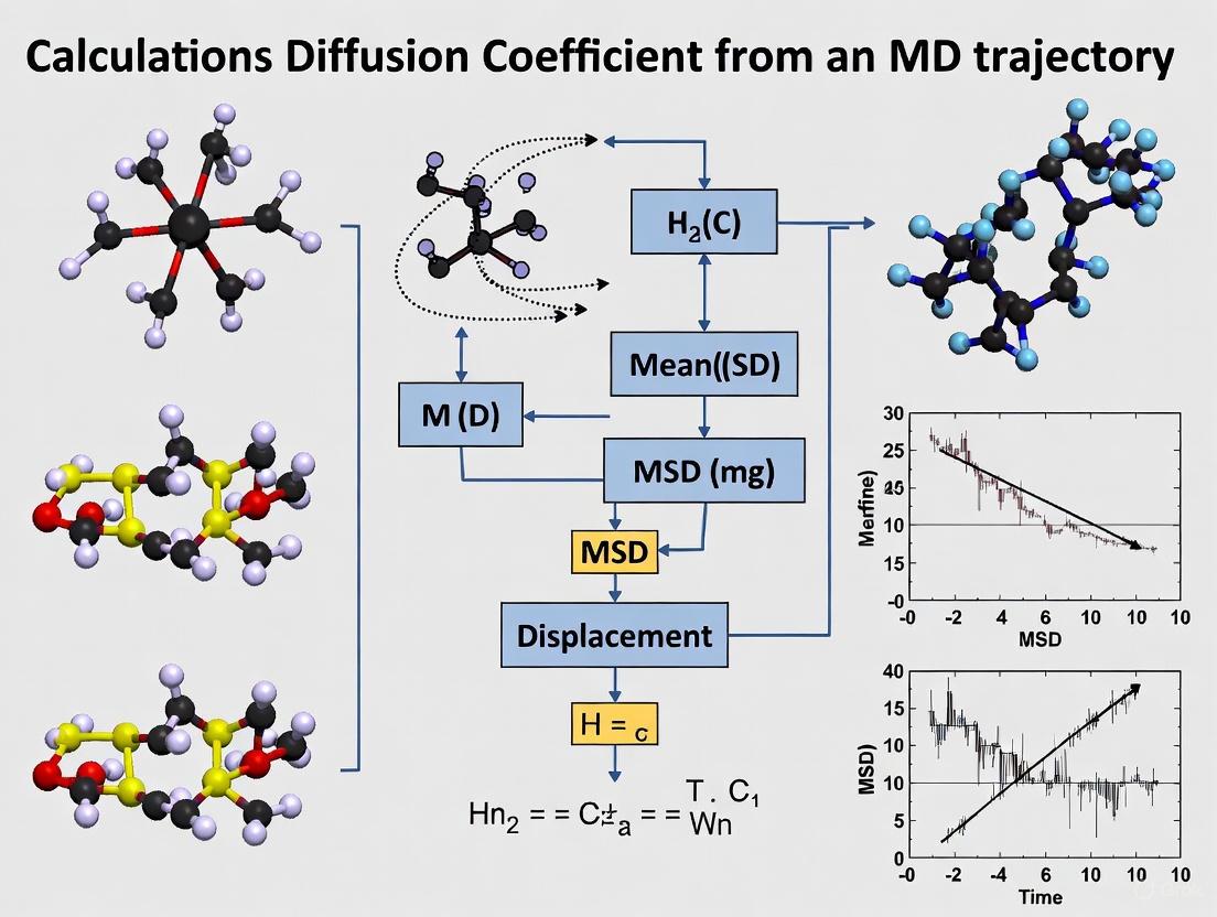
Diagram 1: MSD Workflow for D Calculation.

Critical Considerations for MD Calculations

• Sampling and Convergence: Reliable calculation of a diffusion coefficient, especially for solutes at infinite dilution, often requires very long simulation times to achieve good statistics [6]. A strategy of averaging the MSD from multiple short simulations can be an efficient alternative [6].
• Finite-Size Effects: The diffusion coefficient measured in an MD simulation with periodic boundary conditions ((D{PBC})) is biased by hydrodynamic interactions with periodic images. A correction can be applied [8]: [D{\text{corrected}} = D{PBC} + \frac{2.84 kB T}{6 \pi \eta L}] where (k_B) is Boltzmann's constant, (T) is temperature, (\eta) is the solvent viscosity, and (L) is the box size.
• Temperature Dependence: Diffusion coefficients follow the Arrhenius equation, allowing extrapolation from simulations at higher temperatures [7]: [D(T) = D0 \exp(-Ea / kB T)] where (Ea) is the activation energy. Calculating (D) at multiple temperatures enables this extrapolation.

The Scientist's Toolkit: Essential Reagents and Materials

Table 3: Key Research Reagents and Computational Tools

Item / Tool	Function / Description	Relevance to Experiment
Molecular Dynamics Software	Software packages like GROMACS [8] and AMS [7] that perform MD simulations.	Provides the computational engine to simulate the motion of atoms and molecules over time.
Force Field	A set of empirical parameters (e.g., GAFF, AMBER) describing interatomic potentials [6].	Defines the physics of interactions between atoms in the simulation; critical for accuracy.
Thermostat	An algorithm (e.g., Berendsen, Nosé-Hoover) to control temperature during MD [7].	Maintains the system at a constant temperature, essential for the NVT or NPT ensembles.
Trajectory Analysis Tool	Tools like gmx msd in GROMACS [8] or analysis features in AMSmovie [7].	Processes the saved atomic positions from the MD simulation to compute the MSD or VACF.
Visualization Software	Programs like AMSmovie [7] or VMD.	Allows visual inspection of the simulation trajectory and properties like cell volume or temperature.
4-Methoxy-2-nitrophenylthiocyanate	4-Methoxy-2-nitrophenylthiocyanate, CAS:59607-71-5, MF:C8H6N2O3S, MW:210.21 g/mol	Chemical Reagent
7-Hydroxy-2,4-dimethylquinoline	7-Hydroxy-2,4-dimethylquinoline	7-Hydroxy-2,4-dimethylquinoline (C12H11NO3) is a quinoline derivative for research use only (RUO). Explore its applications in medicinal chemistry and drug discovery.

Molecular diffusion is a cornerstone physical process with wide-ranging implications. A deep understanding of its principles, from Fick's macroscopic laws to the microscopic random walk, is indispensable. For modern researchers, molecular dynamics simulations offer a powerful avenue to quantitatively investigate diffusion and calculate diffusion coefficients directly from particle trajectories. Mastering the MSD and VACF methodologies, while accounting for practicalities like finite-size effects and sufficient sampling, enables accurate prediction of this critical transport property, facilitating advances in drug development, material science, and chemical engineering.

The Einstein-Smoluchowski relation represents a cornerstone of statistical physics, establishing a fundamental connection between random microscopic motion and macroscopic diffusion phenomena. First derived independently by Albert Einstein and Marian Smoluchowski in the early 1900s, this relation emerged from theoretical explanations of Brownian motion and provided the first quantitative link between molecular fluctuations and dissipative properties [10]. Its historical significance is profound, as it enabled Perrin's experiments determining Avogadro's number, which ultimately resolved the debate about atomic reality [10].

In contemporary research, this relationship provides the theoretical foundation for extracting transport properties from molecular dynamics (MD) simulations. For computational researchers investigating molecular transport in biological systems or materials science, the Einstein-Smoluchowski relation enables the calculation of diffusion coefficients from particle trajectories, serving as a crucial bridge between atomistic simulations and macroscopic observables [11] [6].

Theoretical Foundations

Fundamental Equations

The classical Einstein-Smoluchowski relation states:

[ D = \mu k_B T ]

Here, (D) represents the diffusion coefficient, (\mu) is the mobility (defined as the ratio of terminal drift velocity to applied force, (\mu = vd/F)), (kB) is Boltzmann's constant, and (T) is absolute temperature [12]. This equation represents one of the first examples of a fluctuation-dissipation relation in statistical physics [10].

For charged particles, the equation takes a more specific form:

[ D = \frac{\muq kB T}{q} ]

where (\mu_q) is the electrical mobility and (q) is the particle charge [12].

Table 1: Special Forms of the Einstein Relation

Equation Name	Formula	Application Context
Classical Einstein-Smoluchowski	(D = \mu k_B T)	General particle diffusion
Electrical Mobility Equation	(D = \frac{\muq kB T}{q})	Charged particles
Stokes-Einstein-Sutherland	(D = \frac{k_B T}{6\pi\eta r})	Spherical particles in liquid
Rotational Diffusion	(Dr = \frac{kB T}{8\pi\eta r^3})	Rotational motion of spheres

Connection to Fick's Laws

The Einstein-Smoluchowski relation provides a kinetic foundation for Fick's laws of diffusion. While Fick's first law:

[ J = -D \frac{dc}{dx} ]

establishes flux (J) as proportional to the concentration gradient, the Einstein-Smoluchowski relation explains the microscopic origin of the diffusion coefficient (D) itself [13]. This connection becomes particularly valuable in MD simulations, where particle displacements can be directly measured and related to macroscopic diffusion through the mean-square displacement (MSD) relation:

[ \langle |\vec{r}(t) - \vec{r}(0)|^2 \rangle = 2nDt ]

where (n) represents dimensionality [6].

Computational Framework for MD Simulations

From Particle Trajectories to Diffusion Coefficients

In molecular dynamics research, the primary methodology for calculating diffusion coefficients involves analyzing mean-square displacement (MSD) of particles over time. The fundamental equation applied is:

[ D = \frac{1}{2n} \lim_{t \to \infty} \frac{d}{dt} \langle |\vec{r}(t) - \vec{r}(0)|^2 \rangle ]

where (n) is the dimensionality (typically 3 for MD simulations) [6]. Practical implementation requires careful attention to statistical convergence, as reliable results demand sufficient sampling of particle trajectories.

The Stokes-Einstein equation provides an alternative approach for spherical particles:

[ D = \frac{k_B T}{6\pi\eta r} ]

where (\eta) is solvent viscosity and (r) is the hydrodynamic radius [14]. This relation enables diffusion coefficient estimation from structural molecular properties, though its accuracy diminishes for non-spherical molecules or complex solvation environments.

Figure 1: MD to Diffusion Coefficient Workflow

Advanced Computational Techniques

For complex systems, researchers employ sophisticated algorithms to extract diffusion tensors. The Milestoning method maps atomically detailed dynamics to kinetics of coarse variables (CV) by partitioning CV space into cells and analyzing transitions between dividers (milestones) [11]. This approach enables efficient computation of diffusion properties even for activated processes.

Kramers-Moyal expansion of the discrete master equation provides another framework for determining space-dependent diffusion tensors from MD simulations [11]. This method calculates rate coefficients between milestones and converts them to potential of mean force and coordinate-dependent diffusion tensors.

Practical Implementation Protocols

MSD-Based Calculation Methodology

The standard protocol for diffusion coefficient calculation from MD trajectories involves:

• Trajectory Preparation: Run MD simulation with appropriate force fields and periodic boundary conditions. For the General AMBER force field (GAFF), simulation boxes of sufficient size must be ensured to minimize finite-size effects [6].

• MSD Computation: Calculate mean-square displacement using: [ \text{MSD}(t) = \langle |\vec{r}(t + t0) - \vec{r}(t0)|^2 \rangle ] where averaging occurs over both time origins ((t_0)) and particles [6].

• Linear Regression: Fit the linear portion of MSD versus time curve to obtain the diffusion coefficient: [ D = \frac{1}{2n} \times \text{slope} ]

• Convergence Validation: Ensure statistical reliability through multiple independent simulations or block averaging [6].

Table 2: Diffusion Coefficient Calculation Methods in MD

Method	Key Equation	Advantages	Limitations
Einstein (MSD)	(D = \frac{1}{6N}\frac{d}{dt}\sum_{i=1}^N \langle	\vec{r}i(t)-\vec{r}i(0)	^2\rangle)	Direct implementation	Requires long trajectories
Green-Kubo	(D = \frac{1}{3}\int_0^\infty\langle\vec{v}(t)\cdot\vec{v}(0)\rangle dt)	Theoretical rigor	Sensitive to noise
Milestoning	(D$ derived from transition rates between milestones [11]	Efficient for rare events	Complex implementation
Stokes-Einstein	(D = \frac{k_B T}{6\pi\eta r})	Simple calculation	Limited to spherical particles

Radius Estimation for Complex Molecules

For non-spherical molecules, the Stokes-Einstein relation requires careful estimation of molecular radius. Research demonstrates two effective approaches [14]:

• Simple Radius ((rs)): Calculated from van der Waals volume (V{vdw}) using: [ rs = \left(\frac{3V{vdw}}{4\pi}\right)^{1/3} ]

• Effective Radius ((re)): Derived from radius of gyration (rg): [ re = \sqrt{\frac{5}{3}} rg \approx 1.29 r_g ]

Studies show that for molecules with strong hydration ability, the effective radius provides superior agreement with experimental data, while for other compounds, the simple radius performs better [14].

Applications in Drug Development and Materials Science

Pharmaceutical Applications

In pharmaceutical research, diffusion coefficients play crucial roles in understanding drug delivery and pharmacokinetics. Passive transport of drug molecules—the driving force behind distribution to organs—directly depends on diffusion rates [14]. Computational estimation of diffusion coefficients provides valuable molecular descriptors for drug screening, especially when experimental measurement proves challenging.

Research demonstrates that theoretical estimation of diffusion coefficients for small drug-like molecules achieves reasonable agreement with experimental values (deviation ~0.3×10⁻⁶ cm²/s) [14]. This accuracy enables preliminary screening of candidate compounds based on transport properties before synthesis.

Biomolecular Systems

For proteins and other macromolecules, diffusion coefficients influence numerous biochemical processes, including protein aggregation and transportation in intercellular media [6]. MD simulations employing the Einstein-Smoluchowski relation can predict diffusion behavior under various thermodynamic conditions, sometimes unreachable by experiments.

Studies show excellent correlation (R² = 0.996) between predicted and experimental diffusion coefficients for proteins in aqueous solutions, validating the computational approach [6].

The Scientist's Toolkit: Essential Research Reagents

Table 3: Essential Computational Tools for Diffusion Coefficient Calculation

Tool/Software	Function	Application Context
AMS Trajectory Analysis [15]	Analyzes MD trajectories, computes MSD, radial distribution functions	Ionic conductivity studies, molecular centers of mass diffusion
LAMMPS [16]	MD simulation package with various force fields	General MD simulations of gases, liquids, biomolecules
General AMBER Force Field (GAFF) [6]	Provides parameters for organic molecules	Drug diffusion studies, biomolecular systems
Milestoning Algorithm [11]	Efficiently computes kinetics in coarse-grained space	Activated processes, rare events
MOE Software System [14]	Calculates stable molecular conformations	Molecular radius estimation for Stokes-Einstein equation
Methyl 2,2-dimethylpent-4-enoate	Methyl 2,2-dimethylpent-4-enoate, CAS:76352-72-2, MF:C8H14O2, MW:142.2 g/mol	Chemical Reagent
2,6-Bis(chloromethyl)naphthalene	2,6-Bis(chloromethyl)naphthalene, CAS:93036-77-2, MF:C12H10Cl2, MW:225.11 g/mol	Chemical Reagent

Current Challenges and Future Perspectives

Despite the well-established theoretical foundation, practical application of the Einstein-Smoluchowski relation in MD simulations faces several challenges. For solutes at infinite dilution, convergence requires exceptionally long simulation times—up to 60-80 nanoseconds for reliable results [6]. This computational demand necessitates efficient sampling strategies, such as averaging MSD from multiple short simulations.

Recent research explores generalizations of the Einstein-Smoluchowski relation for anomalous diffusion systems, where mean-square displacement follows (\langle x^2(t) \rangle \propto t^\alpha) with (\alpha \neq 1) [10]. In such systems, which are common in cellular environments and complex fluids, the classical relation may break down, requiring modified theoretical frameworks.

The integration of machine learning with molecular dynamics promises enhanced prediction of diffusion properties, potentially reducing computational costs while maintaining accuracy. As force fields continue to improve and computational resources expand, the Einstein-Smoluchowski relation will remain fundamental to connecting molecular simulations with experimental observables in increasingly complex systems.

Fick's Laws of Diffusion and Their Molecular Interpretation

Fick's laws of diffusion form the foundational mathematical framework for describing the transport of mass through random molecular motion. First posited by physiologist Adolf Fick in 1855, these laws quantify how particles spread from regions of high concentration to regions of low concentration, ultimately striving toward equilibrium [17]. Fick's work was inspired by earlier experiments of Thomas Graham and developed through studies of salt diffusing between reservoirs through tubes of water [17]. These laws have proven universally applicable across scientific disciplines, describing diffusion in solids, liquids, and gases, and remain cornerstone principles in fields ranging from chemical engineering to pharmaceutical research [17] [18].

The significance of Fick's laws extends beyond mass transport, as they share remarkable mathematical similarity with other fundamental transport equations: Darcy's law for hydraulic flow, Ohm's law for charge transport, and Fourier's law for heat transport [17]. This connection underscores the universal nature of transport phenomena. For researchers investigating molecular dynamics, particularly in drug development where compound diffusion across biological barriers is critical, Fick's laws provide the theoretical basis for extracting quantitative diffusion parameters from computational simulations [7] [6].

Fundamental Principles of Fick's Laws

Fick's First Law: The Steady-State Condition

Fick's first law describes diffusion under steady-state conditions where concentration remains constant with time. It establishes that the diffusive flux is proportional to the negative concentration gradient. In one-dimensional form, it is expressed as [17]:

[ J = -D \frac{\partial \phi}{\partial x} ]

where:

• (J) represents the diffusion flux, measuring the amount of substance flowing through a unit area per unit time (dimensions of mol·m⁻²·s⁻¹ or g·m⁻²·s⁻¹)
• (D) is the diffusion coefficient or diffusivity (dimensions of m²·s⁻¹)
• (\phi) is the concentration (dimensions of mol·m⁻³ or g·m⁻³)
• (x) is the position coordinate
• The negative sign indicates that diffusion occurs down the concentration gradient

For multi-dimensional systems, Fick's first law employs the gradient operator [17]:

[ \mathbf{J} = -D \nabla \phi ]

At the molecular level, Fick's first law can be derived from the random walk of particles. Considering atomic jumps in a crystalline solid, where each plane contains (C\lambda) atoms per unit area, the net flux between adjacent planes with jump frequency (\nu) and jump distance (\lambda) becomes [19]:

[ J = -\frac{1}{6}\nu \lambda^2 \frac{\partial C}{\partial x} ]

This directly correlates to Fick's first law, with the diffusivity (D = \frac{1}{6}\nu \lambda^2) emerging from microscopic molecular parameters [19].

Fick's Second Law: The Time-Dependent Condition

Fick's second law predicts how diffusion causes concentration to change with time, making it essential for non-steady-state processes. In one dimension, it is expressed as [17]:

[ \frac{\partial \phi}{\partial t} = D \frac{\partial^2 \phi}{\partial x^2} ]

where:

• (\frac{\partial \phi}{\partial t}) represents the rate of change of concentration with time

For multi-dimensional systems, Fick's second law utilizes the Laplacian operator [17]:

[ \frac{\partial \phi}{\partial t} = D \nabla^2 \phi ]

This partial differential equation has identical mathematical form to the heat equation, with the diffusion coefficient (D) replacing thermal conductivity [17] [20]. The fundamental solution to this equation for an initial point source is a Gaussian distribution [17]:

[ \phi(x,t) = \frac{1}{\sqrt{4\pi Dt}} \exp\left(-\frac{x^2}{4Dt}\right) ]

Fick's second law can be derived from the first law by considering mass conservation. Applying the continuity equation for mass, which states that the rate of concentration change equals the negative divergence of the flux [20]:

[ \frac{\partial \phi}{\partial t} + \frac{\partial}{\partial x} J = 0 ]

Substituting Fick's first law into this equation yields:

[ \frac{\partial \phi}{\partial t} - \frac{\partial}{\partial x}\left(D\frac{\partial \phi}{\partial x}\right) = 0 ]

Assuming a constant diffusion coefficient (D) allows simplification to the standard form of Fick's second law [20].

Table 1: Key Parameters in Fick's Laws of Diffusion

Parameter	Symbol	Dimensions	Typical Values	Physical Meaning
Diffusion Flux	(J)	[amount of substance]·[length]⁻²·[time]⁻¹	Varies by application	Rate of flow through unit cross-sectional area
Diffusion Coefficient	(D)	[length]²·[time]⁻¹	10⁻¹¹–10⁻¹⁰ m²/s (biological molecules) [17]	Measure of mobility under concentration gradient
Concentration	(\phi)	[amount of substance]·[length]⁻³	Varies by system	Number of molecules per unit volume
Concentration Gradient	(\frac{\partial \phi}{\partial x})	[amount of substance]·[length]⁻⁴	Determines direction and magnitude of flux	Spatial rate of concentration change

Molecular Interpretation of Diffusion

Molecular Origins of Diffusive Behavior

At the molecular level, diffusion results from random thermal motion of particles. In gases and liquids, molecules undergo constant, random collisions that cause them to spread out progressively over time [13]. This random walk process can be quantified through the Einstein-Smoluchowski equation [13]:

[ D = \frac{\lambda^2}{2\tau} ]

where:

• (\lambda) represents the mean free path between collisions
• (\tau) is the mean time between collisions

This equation reveals that the diffusion coefficient depends fundamentally on the molecular step size and frequency. In more complex systems, the Stokes-Einstein relation provides another perspective, connecting diffusion to hydrodynamic properties [13]:

[ D = \frac{kT}{6\pi\eta a} ]

where:

• (k) is Boltzmann's constant
• (T) is absolute temperature
• (\eta) is solvent viscosity
• (a) is the hydrodynamic radius of the diffusing particle

This relationship highlights the inverse dependence of diffusivity on both molecular size and solvent viscosity, explaining why larger molecules diffuse more slowly and why diffusion rates increase with temperature [13].

The driving force for diffusion has been historically attributed to concentration gradients, though research suggests this may be an oversimplification. While Fick originally postulated concentration as the driving force, later scientific consensus shifted toward chemical potential gradients as the true thermodynamic driving force [21]. Recent investigations by Donohue and Aranovich have revealed limitations in both interpretations, particularly in non-ideal systems such as low-pressure gases, nanoporous materials, and systems with significant density gradients [21]. Their work identified "density waves" that create layered molecular buildups—termed the "Batman Profile" due to its distinctive graphical appearance—challenging the classical Fickian model of infinitesimal random molecular steps [21].

Classification of Diffusion Regimes

Diffusion processes are categorized based on their adherence to Fick's laws:

• Fickian (Normal) Diffusion: Processes that obey Fick's laws, typically observed in homogeneous systems under constant conditions [17] [18]
• Non-Fickian (Anomalous) Diffusion: Processes that deviate from Fick's laws, often occurring in complex environments like porous media or polymer systems [17]

The temperature dependence of diffusion follows Arrhenius behavior, expressed as [7]:

[ D = D0 \exp\left(-\frac{Ea}{k_B T}\right) ]

where:

• (D_0) is the pre-exponential factor
• (E_a) is the activation energy for diffusion
• (k_B) is Boltzmann's constant
• (T) is absolute temperature

This relationship enables extrapolation of diffusion coefficients to different temperatures, which is particularly valuable for estimating diffusion rates at physiological conditions from higher-temperature simulations [7].

Figure 1: Relationship between microscopic molecular motion and macroscopic diffusion laws

Calculating Diffusion Coefficients from Molecular Dynamics

Theoretical Framework for MD Diffusion Calculations

Molecular dynamics (MD) simulations provide a powerful approach for calculating diffusion coefficients by tracking the temporal evolution of particle positions and velocities. The diffusion coefficient (D) can be determined through two primary methods derived from different aspects of molecular motion [7].

The Mean Squared Displacement (MSD) method applies the Einstein relation, which states that for three-dimensional diffusion [6]:

[ \langle |\mathbf{r}(t) - \mathbf{r}(0)|^2 \rangle = 6Dt ]

where:

• (\langle |\mathbf{r}(t) - \mathbf{r}(0)|^2 \rangle) represents the ensemble-averaged mean squared displacement
• (\mathbf{r}(t)) is the position at time (t)
• The diffusion coefficient is obtained from the slope of MSD versus time [7]:

[ D = \frac{\text{slope}(MSD)}{6} ]

The Velocity Autocorrelation Function (VACF) method employs the Green-Kubo relation, which connects diffusion to the time integral of velocity correlations [7] [6]:

[ D = \frac{1}{3} \int_{0}^{\infty} \langle \mathbf{v}(0) \cdot \mathbf{v}(t) \rangle dt ]

where:

• (\langle \mathbf{v}(0) \cdot \mathbf{v}(t) \rangle) represents the velocity autocorrelation function
• This approach captures how a particle's velocity correlates with its initial velocity over time

Table 2: Comparison of MD Methods for Diffusion Coefficient Calculation

Method	Fundamental Relation	Advantages	Limitations	Convergence Requirements
Mean Squared Displacement (MSD)	( D = \lim_{t \to \infty} \frac{\langle |\mathbf{r}(t)-\mathbf{r}(0)|^2 \rangle}{6t} )	Intuitive physical interpretation, straightforward implementation	Requires long simulation times for reliable statistics, sensitive to initial conditions	MSD should show clear linear regime; slope should stabilize with increasing simulation time
Velocity Autocorrelation Function (VACF)	( D = \frac{1}{3} \int{0}^{t{\text{max}}} \langle \mathbf{v}(0) \cdot \mathbf{v}(t) \rangle dt )	Faster convergence for some systems, provides additional dynamic information	More sensitive to numerical integration errors, requires high-frequency velocity sampling	Integral should plateau with increasing upper time limit; requires good statistics for velocity correlations

Practical Implementation and Protocols

Implementing MD simulations for diffusion coefficient calculation requires careful attention to system preparation, simulation parameters, and analysis techniques. The following workflow outlines a standardized approach based on established protocols [7]:

System Preparation:

• Initial Structure Acquisition: Import crystal structures from CIF files or generate amorphous structures
• Structure Modification: Insert diffusing species (e.g., Li atoms in electrode materials) using builder tools or Grand Canonical Monte Carlo (GCMC) methods
• Equilibration: Perform geometry optimization with lattice relaxation to stabilize the system
• Amorphous System Generation (if needed): Employ simulated annealing by heating to high temperature (e.g., 1600K) followed by rapid cooling

Production Simulation Setup:

• Thermostat Selection: Use Berendsen or other appropriate thermostats with damping constant of ~100 fs
• Simulation Duration: Typically 100,000+ production steps after equilibration
• Sampling Frequency: Set to 5-10 steps for accurate VACF calculation; can be higher for MSD-only analysis
• Temperature Control: Maintain constant temperature during production run

Analysis Procedure:

• MSD Method:
  • Calculate MSD for the diffusing species
  • Identify linear regime of MSD versus time plot
  • Perform linear fit to MSD curve: ( \text{MSD}(t) = 6Dt + b )
  • Extract (D) from slope: ( D = \text{slope}/6 )

• VACF Method:
  • Compute velocity autocorrelation function: ( \langle \mathbf{v}(0) \cdot \mathbf{v}(t) \rangle )
  • Integrate VACF over time
  • Apply formula: ( D = \frac{1}{3} \int{0}^{t{\text{max}}} \langle \mathbf{v}(0) \cdot \mathbf{v}(t) \rangle dt )

For reliable results, researchers should address several critical considerations. Finite-size effects necessitate simulations with progressively larger supercells followed by extrapolation to the "infinite supercell" limit [7]. Statistical convergence requires sufficient sampling, which can be achieved through either multiple independent trajectories or extended simulation times [6]. For biologically relevant temperatures, Arrhenius extrapolation from multiple elevated temperatures (e.g., 600K, 800K, 1200K, 1600K) may be necessary due to impractical simulation timescales at room temperature [7].

Figure 2: Comprehensive workflow for calculating diffusion coefficients from molecular dynamics simulations

Research Reagent Solutions for Diffusion Studies

Table 3: Essential Materials and Computational Tools for MD Diffusion Studies

Item	Function/Application	Implementation Example	Critical Parameters
Force Fields (GAFF, AMBER, CHARMM, ReaxFF)	Describes interatomic potentials and molecular interactions	ReaxFF for reactive systems (e.g., Li-S batteries) [7]; GAFF for organic molecules [6]	Bond stretching, angle bending, torsion, van der Waals, electrostatic terms
Solvation Modules	Models solvent effects and periodic boundary conditions	Implicit solvent for efficiency; Explicit solvent (TIP3P water) for accuracy [6]	Box size, solvent density, cutoff distances
Thermostats (Berendsen, Nosé-Hoover)	Maintains constant temperature during simulations	Berendsen thermostat with damping constant 100 fs [7]	Coupling strength, temperature ramp rates
Trajectory Analysis Tools	Processes MD output to extract diffusion parameters	AMSmovie for MSD/VACF analysis [7]; Custom scripts for batch processing	Sampling frequency, frame interval, fitting algorithms
System Building Tools	Prepares initial structures with desired composition	Molecular builders with SMILES support [7]; GCMC for optimal insertion	Composition control, spatial distribution, energy minimization

Applications in Pharmaceutical Research

Fick's laws of diffusion provide critical insights for drug development professionals, particularly in understanding passive transport of compounds across biological barriers. The exchange rate of oxygen and carbon dioxide in the lungs across the alveolar membrane follows Fick's first law, which can be expressed as [18]:

[ \text{Diffusion Flux} = -P(c2 - c1) ]

where:

• (P) is the permeability, an experimentally determined membrane 'conductance' for a given gas
• (c2 - c1) is the concentration difference across the membrane

This same principle applies to drug permeation across gastrointestinal barriers, blood-brain barrier, and cellular membranes. For drug delivery system design, Fick's second law helps predict drug release kinetics from controlled-release formulations, where the changing concentration gradient over time dictates release rates [18].

Molecular dynamics simulations enable precise calculation of diffusion coefficients for pharmaceutical compounds, providing insights that complement experimental measurements. For instance, MD studies using the General AMBER Force Field (GAFF) have demonstrated satisfactory prediction of diffusion coefficients for organic solutes in aqueous solution, with average unsigned errors of 0.137 × 10⁻⁵ cm²s⁻¹ [6]. This computational approach allows researchers to screen compound permeability early in drug development, potentially reducing reliance on laborious experimental measurements.

The temperature dependence of diffusion coefficients follows Arrhenius behavior, enabling extrapolation to physiological temperatures [7]:

[ \ln D(T) = \ln D0 - \frac{Ea}{k_B} \cdot \frac{1}{T} ]

This relationship is particularly valuable when direct simulation at 310 K (37°C) is computationally prohibitive due to slow dynamics at physiological temperatures.

Limitations and Advanced Considerations

While Fick's laws provide an excellent foundation for understanding diffusion, researchers must recognize their limitations. The standard formulation assumes constant diffusion coefficients, which is only strictly valid for dilute solutions [22]. In concentrated mixtures, Maxwell-Stefan diffusion more accurately describes the system, where diffusion coefficients become tensors and account for interactions between all chemical species present [22].

Recent research has identified fundamental limitations in Fick's law itself. Donohue and Aranovich demonstrated that neither concentration gradients nor chemical potential gradients fully explain diffusion in all systems [21]. Their work revealed that diffusion includes a wave phenomenon, particularly manifest in low-pressure gases, nanoporous materials, and systems with significant scale disparities [21]. These "density waves" create layered molecular buildups that deviate from the smooth concentration profiles predicted by classical Fickian diffusion.

For complex pharmaceutical systems, non-Fickian diffusion often occurs in polymer-based drug delivery systems, gels, and heterogeneous biological tissues. In these cases, anomalous diffusion models with time-dependent or fractional derivatives may be necessary to accurately describe the observed transport behavior [17] [18].

When implementing MD simulations for diffusion coefficient calculation, researchers should consider:

• Finite-size effects: Diffusion coefficients calculated in small simulation boxes may require extrapolation to infinite system size [7]
• Convergence requirements: Reliable diffusion coefficients necessitate sufficient sampling, achieved through either multiple independent trajectories or extended simulation times [6]
• Force field limitations: Different force fields may yield varying diffusion coefficients, requiring validation against experimental data [6]
• Composition dependence: In concentrated systems, diffusion coefficients become composition-dependent, necessitating specialized approaches like Maxwell-Stefan formulation [22]

Despite these limitations, Fick's laws remain fundamentally important for pharmaceutical researchers, providing the conceptual framework and mathematical foundation for understanding and quantifying molecular transport in drug development applications.

Why MD Simulations are Powerful for Diffusion Coefficient Calculation

Molecular dynamics (MD) simulations have emerged as an indispensable tool for calculating diffusion coefficients (D), providing a unique bridge between microscopic particle motion and macroscopic transport properties. This computational technique enables researchers to obtain this critical parameter by analyzing the trajectories of atoms and molecules, offering atomic-level insights that are often challenging to acquire experimentally. The power of MD lies in its ability to study diffusion processes under various thermodynamic conditions, including those difficult to achieve in laboratory settings, while also revealing the fundamental molecular mechanisms governing mass transport.

Theoretical Foundations of Diffusion in MD

At the heart of MD-based diffusion coefficient calculations lies the Einstein relation, which connects the macroscopic diffusion coefficient to the microscopic mean squared displacement of particles. This relationship is derived from the statistical mechanics of random walks and Brownian motion, where the mean squared displacement increases linearly with time.

• Mean Squared Displacement: The MSD is a measure of the average squared distance particles travel over time and is central to calculating diffusion coefficients. For a three-dimensional system, the diffusion coefficient is related to the slope of the MSD versus time plot through the equation: D = slope(MSD)/6 [7]. This approach is generally recommended for its straightforward implementation and interpretation.

• Velocity Autocorrelation Function: As an alternative approach, the diffusion coefficient can be obtained through integration of the velocity autocorrelation function using the Green-Kubo relation: D = (1/3)∫₀∞⟨v(0)·v(t)⟩dt [7] [6]. This method theoretically equals the Einstein relation but requires setting the sampling frequency to small values for accurate results.

The diffusion coefficient D is also related to the friction coefficient ξ through the Einstein-Smoluchowski equation: D = kT/ξ, where k is the Boltzmann constant and T is the temperature. The friction coefficient depends on the sizes and shapes of molecules participating in diffusion [6].

Practical Protocols for Diffusion Coefficient Calculation

MSD Method Protocol

The MSD approach is widely regarded as the more accessible and recommended method for calculating diffusion coefficients from MD trajectories:

• Production Simulation: Run a sufficiently long MD simulation at the temperature of interest after proper equilibration. For accurate statistics, production runs of 100,000 steps or more are typically necessary [7].

• Trajectory Sampling: Set an appropriate sample frequency to write atomic positions to disk. A higher sample frequency results in a larger trajectory file but provides better temporal resolution [7].

• MSD Calculation: Compute the MSD for the atoms of interest using the formula: MSD(t) = ⟨[r(0) - r(t)]²⟩, where r(0) and r(t) represent atomic positions at time 0 and time t, respectively, and the angle brackets denote averaging over all atoms and time origins [7].

• Linear Regression: Perform linear fitting on the MSD curve versus time. The diffusion coefficient is then calculated as one-sixth of the slope of this linear region: D = slope(MSD)/6 [7].

Table 1: Key Parameters for MSD-Based Diffusion Coefficient Calculation

Parameter	Recommended Setting	Purpose
Production Steps	100,000+	Ensure sufficient sampling for statistics
Sample Frequency	5-10 steps	Balance temporal resolution and file size
Equilibration Period	10,000 steps	Allow system to reach equilibrium
MSD Time Origin	Multiple starting points	Improve averaging and statistics

VACF Method Protocol

The VACF method provides an alternative approach with its own procedural requirements:

• Velocity Tracking: Configure the MD simulation to save atomic velocities at regular intervals by setting an appropriate sampling frequency [7].

• VACF Computation: Calculate the velocity autocorrelation function as: VACF(t) = ⟨v(0)·v(t)⟩, where v(0) and v(t) are velocity vectors at time 0 and time t [6].

• Integration: Integrate the VACF over time to obtain the diffusion coefficient: D = (1/3)∫₀ᵗ⁼ᵗᵐᵃˣ VACF(t)dt [7] [6].

• Convergence Check: Ensure the integral converges to a stable value with increasing tmax [7].

Workflow Visualization

The following diagram illustrates the complete workflow for calculating diffusion coefficients using both primary methods:

Critical Considerations and Methodological Refinements

Addressing Computational Challenges

Several technical challenges must be addressed to ensure accurate diffusion coefficient calculations:

• Finite-Size Effects: The diffusion coefficient depends on the size of the simulation cell due to periodic boundary conditions. Typically, simulations should be performed for progressively larger supercells with extrapolation to the "infinite supercell" limit [7].

• Sampling Strategies: For solutes at infinite dilution, where only one solute molecule exists in a simulation box, reliable prediction of diffusion coefficients requires exceptionally long MD simulations. An efficient sampling strategy involves averaging the MSD collected in multiple short MD simulations rather than relying on a single extended simulation [6].

• Ballistic Regime: At very short time scales, particles exhibit ballistic motion before transitioning to diffusive behavior. Enhanced techniques that isolate this ballistic stage and apply thermodynamic corrections have been developed to refine estimates [23].

Temperature Dependence and Extrapolation

Calculating diffusion coefficients at low temperatures would require prohibitively long simulations to observe sufficient diffusion events. However, MD enables efficient estimation through studies at elevated temperatures followed by extrapolation using the Arrhenius equation:

D(T) = D₀exp(-Eₐ/kBT)

lnD(T) = lnD₀ - (Eₐ/kB) × (1/T)

where D₀ is the pre-exponential factor and Eₐ is the activation energy. The activation energy and pre-exponential factors can be obtained from an Arrhenius plot of ln(D(T)) against 1/T. This approach requires calculating trajectories for at least four different temperatures for each system [7].

Table 2: Comparison of Diffusion Coefficient Calculation Methods

Aspect	MSD Method	VACF Method
Theoretical Basis	Einstein relation	Green-Kubo relation
Primary Data	Atomic positions	Atomic velocities
Computational Cost	Moderate	Moderate to High
Convergence	Good with sufficient sampling	Can be slower
Recommended Use	General purpose	Specialized studies
Key Formula	D = lim(t→∞) ⟨⎸r(t)-r(0)⎸²⟩/6t	D = (1/3)∫₀∞⟨v(0)·v(t)⟩dt

Essential Software Tools and Analysis Libraries

The MD community has developed sophisticated software packages specifically designed for trajectory analysis and diffusion coefficient calculation:

• AMSMovie: Integrated within the AMS package, this tool provides dedicated functions for calculating MSD and diffusion coefficients. It allows users to select specific atom types, set appropriate time windows, and automatically generate diffusion coefficient plots [7].

• MDTraj: A modern, lightweight, and fast software package for analyzing MD simulations. It reads and writes trajectory data in various formats and provides numerous analysis capabilities with interoperability with the Python scientific ecosystem [24].

• GROMACS: A complete modeling package that includes fast molecular dynamics and extensive trajectory analysis utilities. It is particularly known for high performance and comprehensive analysis tools [25] [26].

• YASARA: A complete molecular graphics and modeling program that includes interactive molecular dynamics simulations and analysis capabilities. It can automatically generate detailed scientific reports with plots and tables ready for publication [27].

The Scientist's Toolkit: Essential Research Reagents

Table 3: Essential Software Tools for MD Diffusion Studies

Tool Name	Primary Function	Key Features	License
GROMACS [25] [26]	MD simulation & analysis	High performance MD, comprehensive analysis tools	Free open source (GNU GPL)
AMBER [25] [26]	MD simulation & analysis	Biomolecular focus, well-validated force fields	Proprietary, Free open source
NAMD [25] [26]	MD simulation	Parallel computing, CUDA support	Free academic use
LAMMPS [25]	MD simulation	Soft and solid-state materials, coarse-grain	Free open source
MDTraj [24]	Trajectory analysis	Python interoperability, wide format support	Open source
VMD [25]	Visualization & analysis	Extensive plugin ecosystem, publication-quality rendering	Free academic use
YASARA [27]	Modeling & analysis	Automated scientific reports, easy customization	Proprietary
5,6,7,8-Tetrahydroisoquinolin-5-ol	5,6,7,8-Tetrahydroisoquinolin-5-ol|CAS 97112-03-3	High-purity 5,6,7,8-Tetrahydroisoquinolin-5-ol for research. A key synthetic intermediate for pharmaceuticals and catalysis. For Research Use Only. Not for human or veterinary use.	Bench Chemicals
5-Bromo-3-chloro-2-fluorotoluene	5-Bromo-3-chloro-2-fluorotoluene, CAS:1160574-49-1, MF:C7H5BrClF, MW:223.47	Chemical Reagent	Bench Chemicals

Applications Across Scientific Domains

The capability to calculate diffusion coefficients using MD simulations has enabled advances across multiple scientific disciplines:

• Battery Research: MD simulations with the ReaxFF engine have been used to compute diffusion coefficients of lithium ions in cathode materials like Liâ‚€.â‚„S, providing critical insights for battery optimization and design [7].

• Biomedical Applications: Accurate prediction of diffusion coefficients for proteins and other macromolecules is crucial for understanding biochemical processes such as protein aggregation and transportation in intercellular media [6].

• Materials Design: MD simulations facilitate the study of diffusion in diverse systems, from carbon sequestration applications to industrial process design, often under conditions that are challenging to probe experimentally [23].

• Drug Development: Diffusion properties of drug molecules through membranes and biological barriers can be predicted using MD, providing valuable information for pharmacokinetic optimization [6].

The visualization challenges associated with analyzing these complex MD trajectories have prompted the development of advanced visualization techniques, including virtual reality environments and web-based tools that facilitate intuitive exploration of diffusion pathways and molecular mobility [28].

Molecular dynamics simulations provide a powerful framework for calculating diffusion coefficients by directly connecting atomic-level motion with macroscopic transport properties. The combination of theoretical rigor, practical computational tools, and methodological refinements has established MD as an essential approach for determining this critical parameter across scientific disciplines. As MD methodologies continue to advance with improved force fields, enhanced sampling algorithms, and more sophisticated analysis capabilities, the precision and applicability of diffusion coefficient calculations will further expand, enabling new discoveries in materials science, biochemistry, and pharmaceutical development.

Key Physical Factors Influencing Molecular Diffusion in Biological Systems

Molecular diffusion constitutes a fundamental transport mechanism governing numerous biological processes, from intracellular signaling to drug delivery. This technical guide provides an in-depth analysis of the key physical factors influencing molecular diffusion in biological systems, with particular emphasis on methodologies for calculating diffusion coefficients from molecular dynamics (MD) trajectories. We synthesize current computational approaches, physical models, and experimental validation techniques relevant to researchers and drug development professionals. The article further presents detailed protocols for MD-based diffusion analysis and introduces visualization frameworks for understanding complex diffusional relationships in crowded cellular environments.

In biological systems, macromolecules are constantly moving through diffusion, which plays a fundamental role in processes ranging from protein-ligand binding and folding to intracellular transport and signaling [29]. Understanding how molecules find their binding partners, navigate the crowded cellular environment, and how their diffusional properties influence biological function represents a significant research focus in computational biophysics [29]. Molecular diffusion describes the spread of molecules through random motion driven by thermal energy, with the rate of movement being a function of temperature, fluid viscosity, and particle size and density [1]. This review systematically examines the physical factors governing molecular diffusion and provides researchers with methodologies for quantifying diffusion coefficients using molecular dynamics simulations, a crucial capability for predicting molecular behavior in biological contexts and pharmaceutical applications.

Key Physical Factors Governing Molecular Diffusion

The diffusional behavior of molecules in biological systems is influenced by several interconnected physical factors. These factors collectively determine the mobility, encounter rates, and ultimately the biological activity of molecular species.

Table 1: Key Physical Factors Influencing Molecular Diffusion

Factor	Physical Effect	Impact on Diffusion Coefficient
Temperature	Increases thermal kinetic energy of molecules	Increases diffusion coefficient (linear relationship via Einstein-Smoluchowski equation D = kT/ξ) [6] [1]
Viscosity	Determines magnitude of frictional resistance	Inverse relationship with diffusion coefficient (D ∝ 1/η) [6] [1]
Molecular Size/Shape	Affects hydrodynamic radius and drag	Larger size reduces diffusion (D ∝ 1/R for spherical particles) [1]
Crowding Concentration	Increases collision frequency and steric hindrance	Decreases effective diffusion coefficient [29]
Electrostatic Interactions	Creates attractive/repulsive forces between molecules	Can either enhance or reduce encounter rates depending on charge complementarity [29]
Hydrodynamic Interactions	Mediates long-range coupling through solvent flow	Generally enhances diffusion, particularly important in crowded environments [29]

The diffusion coefficient (D) quantifies the rate of molecular diffusion and can be calculated through multiple theoretical frameworks. The Einstein-Smoluchowski equation relates D to the friction coefficient ξ: D = kT/ξ, where k is Boltzmann's constant and T is temperature [6] [1]. Alternatively, from a microscopic perspective, D can be derived from the mean-square displacement (MSD) of particles over time: ⟨∣r̄ - r̄₀∣²⟩ = 2nDt, where n is the dimensionalty (typically 3 for biological systems) [6]. This relationship provides the foundation for calculating diffusion coefficients from molecular dynamics trajectories.

Calculating Diffusion Coefficients from MD Trajectories

Molecular dynamics simulations enable the calculation of diffusion coefficients through statistical analysis of particle trajectories. Two primary methodologies dominate this approach: Einstein-based MSD analysis and Green-Kubo formalism.

Mean-Square Displacement (MSD) Analysis

The most common approach for calculating diffusion coefficients from MD trajectories relies on the Einstein relation, which connects macroscopic diffusion to microscopic particle displacements [6]. The method involves calculating the mean-square displacement of particles over time:

[ \text{MSD}(t) = \langle | \mathbf{r}(t) - \mathbf{r}(0) |^2 \rangle = 2nDt ]

where (\mathbf{r}(t)) is the position at time t, n is the dimensionality, and D is the diffusion coefficient [6]. In three dimensions (n=3), the relationship becomes MSD(t) = 6Dt, allowing D to be estimated as one-sixth of the slope of the MSD versus time plot in the linear regime [6].

Table 2: Comparison of Methods for Calculating Diffusion Coefficients from MD

Method	Theoretical Basis	Calculation Approach	Advantages/Limitations
MSD Analysis	Einstein relation	Linear regression of MSD(t) vs time	Intuitive but requires long simulations for convergence [6]
Green-Kubo	Velocity autocorrelation	Integration of ⟨v(t)·v(0)⟩	Theoretically equivalent but different statistical properties [6]
Finite-Difference Fitting	Fick's second law	Matching MD concentration profiles to continuum models	Can provide estimates without extremely long trajectories [30]

A significant challenge in MD-based diffusion coefficient calculation is the convergence problem, particularly for solutes at low concentrations. As demonstrated in studies of benzene in ethanol and phenol in water, reliable values of diffusion coefficients may not be obtained even after 60-80 nanoseconds of simulation time [6]. This has led to the development of efficient sampling strategies that average MSD data collected from multiple short MD simulations rather than relying on single extremely long trajectories [6].

Practical Considerations for MD Simulations

Accurate calculation of diffusion coefficients requires careful attention to MD simulation protocols. The following factors significantly impact results:

• System Size and Periodic Boundary Conditions: Simulation boxes must be sufficiently large to minimize periodic image artifacts. A common approach involves defining a cubic box with edges approximately 1.4 nm from the protein periphery [31].

• Solvation: Physiological environment must be mimicked through explicit solvation. The solvate command in packages like GROMACS adds required water molecules, after which counterions are introduced to neutralize system charge [31].

• Trajectory Analysis: Tools like YASARA [27] and AMS Analysis [15] can process MD trajectories to compute MSD and other diffusional properties. These tools typically include options for atom selection, trajectory range specification, and convergence checks through block averaging [15].

Experimental Protocols for MD-Based Diffusion Analysis

Basic Workflow for MD Simulation of Proteins

This protocol outlines the key stages for setting up and running MD simulations for diffusion analysis [31]:

• System Setup

  • Obtain protein coordinates from RCSB PDB and convert to MD-specific format (e.g., .gro for GROMACS)
  • Generate topology file containing molecular parameters, bonding, and force field information
  • Select appropriate force field (e.g., ffG53A7 for proteins with explicit solvent)

• Simulation Environment

  • Define periodic boundary conditions using editconf to create a simulation box
  • Solvate the system using solvate command to add explicit water molecules
  • Neutralize system charge by adding appropriate counterions using genion

• Production Run and Analysis

  • Energy minimization and equilibration before production MD
  • Run production simulation with appropriate timestep and duration
  • Extract trajectories for MSD analysis using tools like gmx msd or custom scripts

Advanced Method: Hybrid MD/Continuum Approach

An innovative approach for estimating diffusion coefficients combines MD simulations with continuum modeling [30]:

• MD Simulation Setup

  • Perform MD simulations of the system using software like LAMMPS with appropriate force fields
  • For gas systems, use Lennard-Jones potentials; for biomolecules, employ specialized force fields

• Continuum Model Implementation

  • Solve the diffusion equation using finite-difference methods: (\frac{\partial}{\partial t}u(\mathbf{x},t) = D\nabla^2 u(\mathbf{x},t))
  • Implement periodic boundary conditions as described in Eq. 6a [30]

• Parameter Estimation

  • Bin MD particle trajectories to the finite-difference grid
  • Estimate optimal diffusion coefficient by minimizing the difference between binned MD data and finite-difference solution using nonlinear least squares (e.g., Levenberg-Marquardt algorithm) [30]

Visualization of Diffusional Processes and Relationships

Workflow for MD-Based Diffusion Coefficient Calculation

Factors Influencing Molecular Diffusion in Biological Systems

Research Reagent Solutions

The following table details essential computational tools and parameters for MD-based diffusion studies:

Table 3: Essential Research Reagents and Computational Tools for MD Diffusion Studies

Item	Function/Purpose	Examples/Notes
MD Software Suites	Engine for running molecular dynamics simulations	GROMACS [31], LAMMPS [30], AMS [15], YASARA [27]
Force Fields	Describes interatomic forces and system physics	AMBER/GAFF [6], CHARMM, Martini (coarse-grained)
Solvation Models	Mimics physiological aqueous environment	TIP3P, SPC water models [6]
Trajectory Analysis Tools	Extracts diffusional properties from MD trajectories	GROMACS analysis tools, YASARA [27], AMS Analysis [15]
Visualization Software	Enables inspection of structures and trajectories	RasMol [31], VMD, PyMOL
Specialized Analysis	Implements specific diffusion coefficient algorithms	BrownDye [29], SDA [29], BD_BOX [29]

Molecular diffusion in biological systems is governed by a complex interplay of physical factors including molecular properties, solvent characteristics, and environmental conditions. Molecular dynamics simulations provide a powerful approach for calculating diffusion coefficients and understanding these relationships at atomic resolution. The MSD analysis method, while computationally demanding, offers a direct route to diffusion coefficients from particle trajectories. Advances in simulation methodologies, including Brownian dynamics and hybrid continuum-MD approaches, continue to enhance our ability to model diffusion in biologically relevant crowded environments. A comprehensive understanding of these factors and methodologies is essential for researchers investigating molecular transport in biological systems and developing computational approaches for drug discovery and development.

Practical Implementation: MSD and VACF Methods with Code Examples

The Mean Squared Displacement (MSD) method, rooted in the seminal work of Einstein and Smoluchowski on Brownian motion, is a cornerstone technique for quantifying particle diffusion and calculating transport properties from Molecular Dynamics (MD) trajectories [10]. The Einstein formulation provides a direct relationship between the random walk of particles at the microscopic level and macroscopic diffusion coefficients. Within the broader context of thesis research on calculating diffusion coefficients from MD, mastering the practical application of the MSD method is fundamental. This technical guide provides researchers, scientists, and drug development professionals with an in-depth understanding of the Einstein formulation's practical implementation, covering the core theory, computational protocols, data analysis, and critical considerations for obtaining reliable diffusion data.

Theoretical Foundation

The Einstein Relation

The foundation of the MSD method is the Einstein relation, which connects the macroscopic diffusion coefficient (D) to the ensemble average of particle displacements [32]. For a three-dimensional system, the relation is expressed as:

[ D = \frac{1}{6} \lim_{t \to \infty} \frac{d}{dt} \langle | \mathbf{r}(t) - \mathbf{r}(0) |^2 \rangle ]

Here, (\mathbf{r}(t)) represents the position of a particle at time (t), and the angle brackets (\langle \cdot \rangle) denote the ensemble average over all particles and time origins [33] [6]. The term (\langle | \mathbf{r}(t) - \mathbf{r}(0) |^2 \rangle) is the MSD. For normal (Brownian) diffusion in an isotropic medium, the MSD increases linearly with time, and the diffusion coefficient is proportional to the slope of this linear relationship. The factor of 6 accounts for the three spatial dimensions (a factor of 2 per dimension) [7].

The Einstein-Smoluchowski relation further connects diffusion to mobility, forming a fundamental fluctuation-dissipation theorem [10]. This states that the diffusion coefficient (D), mobility (\mu), and temperature (T) are related by:

[ \mu = \frac{D}{k_B T} ]

where (k_B) is the Boltzmann constant. While this guide focuses on the diffusion coefficient, this relationship underpins the broader significance of MSD calculations in understanding transport phenomena.

MSD Formulations and Dimensionality

The general expression for the MSD of a particle over a time lag (\tau) is given by [33]:

[ MSD(\tau) = \bigg{\langle} \frac{1}{N} \sum{i=1}^{N} |\mathbf{r}i(\tau) - \mathbf{r}_i(0)|^2 \bigg{\rangle} ]

where (N) is the number of particles, and (\mathbf{r}_i) are their coordinates. The MSD can be calculated for specific dimensional components depending on the system of interest [33]. For example, surface diffusion might require a 2D MSD in the xy-plane. The dimensionality factor (d) in the denominator of the Einstein relation ((2d)) must match the MSD's dimensionality: (d=3) for 'xyz' (3D), (d=2) for 'xy', 'yz', or 'xz' (2D), and (d=1) for 'x', 'y', or 'z' (1D) [33].

Table 1: Diffusion Coefficient Formulas for Different Dimensionalities

MSD Type	Dimensionality (d)	Einstein Relation (D = ...)
3D ('xyz')	3	( \frac{slope}{6} )
2D (e.g., 'xy')	2	( \frac{slope}{4} )
1D (e.g., 'x')	1	( \frac{slope}{2} )

Computational Methodology

Essential Preprocessing of MD Trajectories

A critical prerequisite for a correct MSD calculation is the use of unrapped coordinates [33]. MD simulations typically use periodic boundary conditions, and atoms that cross the box boundary are "wrapped" back into the primary cell. Using these wrapped coordinates for MSD analysis will result in incorrect, artificially small displacements. Therefore, the trajectory must be preprocessed to produce an "unwrapped" trajectory, where atoms maintain their continuity of motion across periodic images. Some simulation packages, like GROMACS, provide tools for this (e.g., gmx trjconv -pbc nojump) [33] [34].

Furthermore, the trajectory must be properly equilibrated. The initial portion of the simulation, before the system reaches equilibrium, should be discarded before analysis to avoid biased results [35]. The choice of time interval between saved frames in the trajectory ((\Delta t)) is also crucial. It must be small enough to capture the relevant dynamics but not so small as to create overly large trajectory files. A good practice is to save coordinates at intervals on the order of the picosecond timescale for typical molecular systems [7].

MSD Calculation Algorithms

There are two primary algorithms for computing the MSD from a discrete trajectory: the simple windowed algorithm and the Fast Fourier Transform (FFT)-based algorithm.

• Windowed Algorithm: This direct method calculates the MSD for a series of time lags ((\tau)) by averaging the squared displacements over all possible time origins within the trajectory [33]. While conceptually straightforward, this algorithm has a computational cost that scales with (O(N^2)), where (N) is the number of frames, making it slow for very long trajectories.

• FFT-Based Algorithm: This is a more advanced and computationally efficient method that leverages FFT to compute the MSD with (O(N \log N)) scaling [33]. This algorithm is recommended for long trajectories due to its superior speed. It is implemented in libraries like tidynamics and can be accessed in analysis tools like MDAnalysis by setting fft=True [33].

The following workflow diagram illustrates the key steps in a robust MSD calculation protocol.

Linear Fitting and the Diffusion Coefficient

Once the MSD is computed, the self-diffusivity is determined by fitting a straight line to the MSD versus time lag curve [33] [34]. The slope of this line is equal to (2dD), where (d) is the dimensionality.

• Selecting the Linear Regime: Visual inspection of the MSD plot is essential [33]. The MSD is often not linear across all time lags. At very short time lags, particle motion may be ballistic (MSD (\propto t^2)), while at very long time lags, the MSD may become noisy due to poor averaging [33] [36]. The linear segment representing pure diffusion is the "middle" part of the MSD curve. A log-log plot of MSD versus time can help identify this regime, as it will have a slope of 1 for normal diffusion [33].
• Fitting Procedure: A linear model is fitted to the selected linear segment of the MSD. For example, using scipy.stats.linregress in Python [33]:

The GROMACS gmx msd module automates this fitting, with options -beginfit and -endfit to define the fitting range. By default (-beginfit -1 and -endfit -1), it fits from 10% to 90% of the total time lag [34].

Practical Implementation and Tools

Software Solutions for MSD Analysis

Several software packages commonly used in MD research provide robust implementations for MSD analysis. The table below summarizes key features and considerations.

Table 2: Comparison of MSD Analysis Software Tools

Software/Tool	MSD Command / Class	Key Features and Considerations
MDAnalysis	analysis.msd.EinsteinMSD	Python library. Supports windowed and FFT algorithms (fft=True). Requires tidynamics for FFT. Mandatory unwrapped coordinates [33].
GROMACS	gmx msd	Command-line tool. Integrates with GROMACS workflow. Automates linear fitting. Can calculate diffusion per molecule (-mol) [34].
ASE (Atomic Simulation Environment)	md.analysis.DiffusionCoefficient	Python library. Can calculate for specific atoms or molecules (using center of mass). Allows trajectory segmentation for statistics [35].
AMS	MD Properties → MSD	GUI-based in AMSmovie. Directly plots MSD and calculates D from the slope [7].

A Scientist's Toolkit for MSD Analysis

This table details essential "research reagents" – the computational tools and data components required for a successful MSD experiment.

Table 3: Essential Computational Materials for MSD Analysis

Item	Function and Specification
Unwrapped Trajectory File	The primary input data. Typically in formats like XTC, TRR, or DCD. Must contain unwrapped particle coordinates to ensure correct displacement calculations [33].
Topology File	Defines the system structure (e.g., TPR, GRO, PDB). Used to select atom groups for analysis [34].
Index File (Optional)	A file (e.g., GROMACS .ndx) specifying groups of atoms or molecules for which the MSD will be computed separately [34].
FFT MSD Library (e.g., tidynamics)	A Python package that enables fast (O(N \log N)) MSD computation. Crucial for handling long trajectories efficiently [33].
Linear Regression Function	A tool (e.g., scipy.stats.linregress, numpy.linalg.lstsq) for performing the linear fit on the MSD data to extract the slope and, consequently, D [33] [35].
N-(Azetidin-3-yl)quinazolin-4-amine	N-(Azetidin-3-yl)quinazolin-4-amine, CAS:1380300-68-4, MF:C11H12N4, MW:200.24
4-(2-(2-Ethoxyethoxy)ethoxy)aniline	4-(2-(2-Ethoxyethoxy)ethoxy)aniline|95%|CAS 90688-48-5

Advanced Considerations and Validation

Error Estimation and Statistical Reliability

Obtaining a reliable diffusion coefficient requires careful statistical analysis. A single, short MD simulation often provides poor statistics. Two common strategies to improve reliability are:

• Averaging over Multiple Segments: The trajectory can be divided into multiple segments (blocks), and the MSD/D is calculated for each segment. The final reported D is the average over all segments, and the standard deviation provides an error estimate [35].
• Averaging over Multiple Runs: For solutes at infinite dilution, where only one molecule is present in the simulation box, a single long trajectory may be insufficient. An efficient sampling strategy is to run multiple independent simulations and average the MSDs collected from these short runs [6].

The GROMACS gmx msd tool provides an error estimate based on the difference in diffusion coefficients obtained from fits over the first and second halves of the fit interval [34].

Common Pitfalls and How to Avoid Them

Several factors can lead to inaccurate MSD results:

• Finite-Size Effects: The calculated diffusion coefficient can depend on the size of the simulation box due to hydrodynamic interactions with periodic images [6]. Typically, simulations are performed for progressively larger supercells, and the diffusion coefficients are extrapolated to the "infinite supercell" limit [7].
• Anomalous Diffusion: In complex environments like crowded proteins or polymer matrices, diffusion may be anomalous, where the MSD scales as (\text{MSD} \propto t^{\alpha}) with (\alpha \ne 1) [36] [10]. In such cases, the standard Einstein relation does not apply directly, and the analysis must account for the anomalous exponent (\alpha).
• Memory and Performance: MSD calculation, especially the windowed method, is memory-intensive for long trajectories. Using the FFT-based algorithm or restricting the maximum time lag for analysis (e.g., with -maxtau in gmx msd) can mitigate this [33] [34].

The Mean Squared Displacement method, via the Einstein formulation, is a powerful and widely used technique for extracting diffusion coefficients from molecular dynamics trajectories. Its successful application in research, including drug development where understanding molecular mobility is critical, depends on a rigorous practical workflow: using unwrapped trajectories, selecting an efficient computational algorithm, carefully identifying the linear regime of the MSD plot, and performing robust statistical analysis to estimate errors. Adherence to these detailed protocols ensures the production of reliable, reproducible diffusion data that can validly inform scientific conclusions and models.

Step-by-Step MSD Calculation from Trajectory Data

Theoretical Foundation: The Einstein Relation

The Mean Squared Displacement (MSD) is a fundamental measure in the analysis of stochastic processes, rooted in the study of Brownian motion. It quantifies the deviation of a particle's position from a reference position over time and provides a direct pathway to calculating the self-diffusion coefficient, D [37] [38].

For a particle undergoing random Brownian motion in an isotropic medium, the MSD exhibits a linear relationship with time. The Einstein relation formalizes this, stating that the MSD for a d-dimensional diffusion process is given by [37] [38]: [MSD(t) = \langle | \vec{r}(t) - \vec{r}(0) |^{2} \rangle = 2dDt] where:

• (\vec{r}(t)) is the position vector of the particle at time (t).
• (d) is the dimensionality of the diffusion (e.g., 1, 2, or 3).
• (D) is the self-diffusion coefficient.
• The angle brackets (\langle \rangle) denote an ensemble average, typically performed over all particles of the same type and/or over multiple time origins.

In practice, for a computational system containing (N) equivalent particles, the MSD is calculated from trajectory data using the following Einstein formula [37] [39]: [MSD(r{d}) = \bigg{\langle} \frac{1}{N} \sum{i=1}^{N} |r{d} - r{d}(t0)|^{2} \bigg{\rangle}{t{0}}] Here, the average is taken over all possible time origins ((t0)) and all (N) particles, maximizing statistical accuracy.

Critical Preprocessing of Trajectory Data

A critical and often overlooked step in MSD calculation is the proper preparation of trajectory data. Failure to correctly handle periodic boundary conditions is the most common source of error.

• Unwrapped Coordinates: The MSD calculation requires coordinates in an unwrapped (or "no-jump") convention [37] [39]. When a particle crosses a periodic boundary, it must not be wrapped back into the primary simulation cell. Using wrapped coordinates will cause artificial jumps in the measured particle paths, severely underestimating the true MSD and the resulting diffusion coefficient.
• How to Unwrap Trajectories:
  • In GROMACS, use the gmx trjconv command with the -pbc nojump flag [37] [39].
  • In MDAnalysis, use the NoJump transformation from the MDAnalysis.transformations module [40].

Table: Essential Checks Before MSD Analysis

Checkpoint	Description	Common Pitfalls
Coordinate Convention	Ensure trajectories are unwrapped.	Using wrapped trajectories invalidates results [37].
Trajectory Length	Simulation must be long enough to observe diffusive behavior.	Short trajectories fail to reach linear MSD regime.
Frame Interval	Save frames with a small enough time interval.	Large time steps poorly capture particle motion [37].
Equilibration	Confirm system is equilibrated before analysis.	Analyzing non-equilibrated data introduces artifacts.

Practical Calculation Workflows

Core Calculation Procedure

The general workflow for a "windowed" MSD calculation involves averaging over all possible time origins within the trajectory [37]. For a trajectory with (T) total frames, the MSD at a lag time ( \tau = n \Delta t ) (where ( \Delta t ) is the time between frames) is:

[MSD(\tau) = \frac{1}{T-n} \sum{i=1}^{T-n} \frac{1}{N} \sum{j=1}^{N} \left[ \vec{r}j(t{i+n}) - \vec{r}j(ti) \right]^2]

This calculation is computationally intensive, scaling quadratically with the number of frames. However, Fast Fourier Transform (FFT)-based algorithms can compute the MSD with (N log(N)) scaling, offering dramatic speed improvements for long trajectories [37] [39].

Step-by-Step Implementation in MDAnalysis

The following Python code demonstrates a complete MSD calculation and diffusion coefficient extraction using MDAnalysis [37].

Implementation in GROMACS

In GROMACS, the gmx msd command provides a direct way to compute MSDs and diffusion coefficients [34].

Key gmx msd options for accurate results [34]:

• -trestart: Defines the time between reference points for the MSD calculation (default 10 ps).
• -beginfit / -endfit: Specifies the time range (ps) for the linear fit to the MSD. If set to -1, fitting starts at 10% and ends at 90% of the trajectory.
• -mol: Calculates MSD for individual molecules, providing statistics and error estimates.

Extracting the Diffusion Coefficient

Identifying the Linear Regime

The connection between MSD and the diffusion coefficient (D) is given by [37]: [Dd = \frac{1}{2d} \lim{t \to \infty} \frac{d}{dt} MSD(r_{d})]

In practice, this derivative is obtained by performing a linear least-squares fit to the MSD curve over an appropriate time range. Not all portions of the MSD curve are suitable for this fit:

• Short lag times: May exhibit ballistic, non-diffusive behavior where MSD (\propto t^2).
• Long lag times: Often show high variance and poor averaging due to limited statistics.

Visual inspection is crucial. The linear regime can be confirmed by viewing the MSD on a log-log plot, where the diffusive regime will have a slope of 1 [37].

Performing the Linear Fit

Once the linear region is identified, the diffusion coefficient is calculated from the slope of the fit [37].

Table: MSD Linear Fit Parameters for Common Diffusion Types

MSD Type	Dimensionality (d)	Einstein Relation	Slope for D=1×10⁻⁵ cm²/s
x (1D)	1	(MSD = 2Dt)	2×10⁻⁵
xy (2D)	2	(MSD = 4Dt)	4×10⁻⁵
xyz (3D)	3	(MSD = 6Dt)	6×10⁻⁵

Advanced Considerations & Best Practices

Error Estimation and Statistical Accuracy

• Combining Replicates: For better statistics, run multiple independent simulations and average the MSDs before fitting, rather than concatenating trajectories [37].
• Error from Fit: The standard error of the slope from linear regression provides an estimate of uncertainty [37] [34].
• Optimal Fitting Points: The optimal number of MSD points for fitting depends on trajectory length and localization uncertainty [41]. Using too many points at long lag times with poor statistics can degrade the quality of the fit.

Table: Key Software Tools for MSD Analysis

Tool	Primary Function	Key Features
MDAnalysis	Python library for trajectory analysis	Flexible EinsteinMSD class with FFT option; customizable selection and dimensionality [37].
GROMACS	MD simulation and analysis	Integrated gmx msd tool; efficient handling of large trajectories; error estimation [34].
tidynamics	Lightweight Python library	Fast FFT-based MSD implementation; used as backend by MDAnalysis [37].
AMS Trajectory Analysis	MD analysis suite	Calculates MSD for molecular centers of mass; includes ionic conductivity computation [15].

Common Pitfalls and Troubleshooting

• Non-linear MSD: If the MSD is not linear, the system may not be purely diffusive, or the observation time may be insufficient to reach the diffusive regime.
• Finite-Size Effects: Diffusion coefficients from simulations with periodic boundary conditions require finite-size corrections, particularly for small system sizes [39].
• Localization Uncertainty: In single-particle tracking experiments, localization error affects short-time MSD behavior and must be accounted for in the analysis [41].

Applications in Drug Development

The MSD and derived diffusion coefficients are critical in pharmaceutical research, particularly in studying drug transport through biological barriers. For example, measuring the diffusion of asthma drugs like theophylline and albuterol through artificial mucus layers provides insights into their efficacy and informs drug design strategies [42]. Experimental diffusion coefficients for these drugs were found to be 6.56 × 10⁻⁶ cm²/s and 4.66 × 10⁻⁶ cm²/s, respectively, values that can be validated and explored further through molecular dynamics simulations [42].

By following this detailed guide, researchers can reliably compute Mean Squared Displacement from molecular dynamics trajectories and extract accurate diffusion coefficients, providing valuable insights into molecular mobility for applications ranging from materials science to pharmaceutical development.

The Green–Kubo relations provide the exact mathematical expression for calculating transport coefficients from the microscopic dynamics of a system at equilibrium. These relations, established by Melville S. Green in 1954 and Ryogo Kubo in 1957, form a cornerstone of linear response theory in statistical mechanics [43]. They enable the prediction of macroscopic transport phenomena—such as diffusion, viscosity, and thermal conductivity—by analyzing the fluctuations that occur naturally in systems at thermal equilibrium. The fundamental insight offered by this formalism is that the relaxations resulting from random fluctuations at equilibrium are indistinguishable from those caused by weak external perturbations [43].

This technical guide focuses specifically on the application of Green–Kubo relations for calculating diffusion coefficients from molecular dynamics (MD) trajectories, a crucial methodology for researchers investigating molecular transport in materials science, drug development, and chemical engineering. The formalism allows for the computation of transport coefficients without perturbing the system out of equilibrium, making it particularly valuable for MD simulations where maintaining natural system dynamics is essential [43]. Within the broader context of thesis research on extracting transport properties from MD trajectories, the Green–Kubo approach provides a rigorous foundation for connecting microscopic atomic motions to macroscopic measurable properties.

Theoretical Foundation

The Green–Kubo Relation for Diffusion

The self-diffusion coefficient ( D ) can be obtained through the Green–Kubo relation that connects it to the velocity autocorrelation function (VACF). The fundamental expression is:

[ D = \frac{1}{3} \int0^\infty \langle \vec{v}i(t) \cdot \vec{v}_i(0) \rangle dt ]

where ( \vec{v}_i(t) ) represents the velocity of particle ( i ) at time ( t ), and the angle brackets ( \langle \cdots \rangle ) denote the ensemble average over all particles and initial times [44]. The factor ( 1/3 ) accounts for the three-dimensional nature of the system in Cartesian coordinates.

The VACF itself measures how a particle's velocity correlates with itself after a time interval ( t ), providing profound insight into the dynamics of the system. In practice, the VACF is calculated as:

[ \text{VACF}(t) = \frac{1}{N} \sum{i=1}^N \langle \vec{v}i(t0 + t) \cdot \vec{v}i(t0) \rangle{t_0} ]

where ( N ) is the number of particles, and the average is taken over all initial times ( t_0 ) and all particles of the same type [45]. This function typically starts positive at ( t=0 ) and often decays to zero, though it may exhibit negative regions indicating back-scattering effects characteristic of cage effects in dense fluids.

Relationship to Other Formulations

The Green–Kubo formalism is mathematically equivalent to the Einstein relation for diffusion, which employs the mean-squared displacement (MSD) of particles:

[ D = \lim{t \to \infty} \frac{1}{6t} \langle | \vec{r}i(t) - \vec{r}_i(0) |^2 \rangle ]

where ( \vec{r}_i(t) ) is the position of particle ( i ) at time ( t ) [44]. While both approaches yield identical diffusion coefficients in the long-time limit, the Green–Kubo method offers advantages in analyzing short-time dynamics and providing insights into the microscopic mechanisms of transport.

Table 1: Key Mathematical Expressions in Green–Kubo Formalism

Quantity	Mathematical Expression	Physical Significance
Self-diffusion Coefficient	( D = \frac{1}{3} \int0^\infty \langle \vec{v}i(t) \cdot \vec{v}_i(0) \rangle dt )	Relates macroscopic transport to microscopic velocity correlations
Velocity Autocorrelation Function	( \text{VACF}(t) = \frac{1}{N} \sum{i=1}^N \langle \vec{v}i(t0 + t) \cdot \vec{v}i(t0) \rangle{t_0} )	Measures memory in velocity fluctuations
Mean-Squared Displacement	( \text{MSD}(t) = \langle	\vec{r}i(t) - \vec{r}i(0)	^2 \rangle )	Quantifies spatial spreading of particles over time
Normalized VACF	( \text{VACF}{\text{norm}}(t) = \frac{ \sumi \langle mi \vec{v}i(t) \cdot \vec{v}i(0) \rangle }{ \sumi \langle mi \vec{v}i^2 \rangle } )	Mass-weighted correlation function normalized to unity at t=0 [45]

Computational Implementation

Calculation Workflow

Implementing the Green–Kubo method for diffusion coefficient calculation from MD trajectories involves a systematic workflow that ensures proper statistical averaging and convergence.

Figure 1: Green–Kubo Calculation Workflow

Step 1: Trajectory Preprocessing – The first step involves loading the MD trajectory and selecting appropriate time ranges for analysis. For meaningful statistics, the trajectory should contain sufficient temporal length to capture the relevant dynamics. The TrajectoryInfo block in analysis tools specifies the trajectory file and frame range [15]:

Step 2: Velocity Extraction – Atomic velocities are extracted from the trajectory file. For multicomponent systems, selection of specific atom types can be performed using element names, region names, or atom indices [15] [45]:

Step 3: VACF Calculation – The velocity autocorrelation function is computed by averaging over all selected atoms and time origins:

[ \text{VACF}(k\Delta t) = \frac{1}{N-k} \sum{i=0}^{N-k-1} \vec{v}i((i+k)\Delta t) \cdot \vec{v}_i(i\Delta t) ]

where ( \Delta t ) is the time step of the trajectory, ( N ) is the total number of steps, and ( k ) ranges from 0 to ( N-1 ) [46].

Step 4: Integration – The running integral of the VACF is computed to obtain the diffusion coefficient as a function of correlation time:

[ I(k\Delta t) = \frac{1}{3} \int0^{k\Delta t} \langle \vec{v}i(\tau) \cdot \vec{v}i(0) \rangle d\tau \approx \frac{\Delta t}{3} \sum{j=0}^k w_j \text{VACF}(j\Delta t) ]

where ( w_j ) are appropriate weighting factors for numerical integration (typically using the trapezoidal rule) [46].

Advanced Computational Considerations

Modern implementations of the Green–Kubo method must address several computational challenges to ensure accurate results:

Statistical Uncertainty Quantification – The kute algorithm (Green–Kubo Uncertainty-based Transport properties Estimator) provides a robust framework for handling uncertainties in the integration process [46]. The uncertainty of the running integral can be estimated as:

[ u(Ik) = \frac{\Delta t}{2} \sqrt{ \sum{i=0}^k \left( u^2(Ci) + u^2(C{i+1}) \right) } ]

where ( u(C_i) ) represents the uncertainty in the VACF at time step ( i ). This uncertainty grows with integration time, making proper weighting essential [46].

Handling Incomplete Convergence – For systems with slow dynamics, such as ionic liquids, the VACF may require exceptionally long simulation times to converge. The weighted average approach for the running transport coefficient addresses this challenge:

[ \gammai = \frac{ \sum{k=i}^N Ik / u^2(Ik) }{ \sum{k=i}^N u^{-2}(Ik) } ]

where the plateau value of ( \gamma_i ) provides the best estimate of the diffusion coefficient [46].

Table 2: Computational Parameters for Green–Kubo Implementation

Parameter	Recommendation	Purpose
Trajectory Length	≥ 5× longest correlation time	Ensure proper decay of VACF to zero
Time Step	0.5-2.0 fs	Adequate resolution of atomic motions
Number of Time Origins	Maximize through block averaging	Improve statistical accuracy
Integration Method	Trapezoidal rule	Balance accuracy and computational cost
Atom Selection	Element-specific or regional	Isolate contributions from different components

Research Toolkit and Applications

Essential Software Tools

Several specialized software packages implement the Green–Kubo methodology for trajectory analysis:

kute – A Python package specifically designed for computing transport properties using the Green–Kubo formalism with built-in uncertainty quantification [46]. This implementation is particularly valuable for systems with complex dynamics where convergence is challenging.

AMS Trajectory Analysis – A standalone program that performs analysis of molecular dynamics trajectories, including VACF calculations and diffusion coefficient estimation [15]. Recent versions have enhanced capabilities for ionic conductivity calculations.

QuantumATK – Includes specialized functions for calculating velocity autocorrelation functions with options for atom selection and mass-weighting [45]:

LAMMPS – The stock LAMMPS code provides capabilities for computing VACF and related transport properties, with options for breaking down contributions by interaction type [47].

Applications in Molecular Systems

The Green–Kubo formalism has been successfully applied to diverse molecular systems, providing insights into transport mechanisms across various scientific domains:

Ionic Liquids – Studies of ethylammonium nitrate (EAN) and other protic ionic liquids have revealed how strong Coulombic interactions lead to sluggish dynamics, requiring extended simulation times for convergence [46]. The formalism has helped elucidate the relationship between molecular structure and transport properties in these customizable materials.

Small Alcohol Systems – Research on ethanol, propanol, ethylene glycol, propylene glycol, and 1,3-propanediol has demonstrated how atomic-level breakdown of Green–Kubo relations reveals competition for thermal conduction between carbon and hydroxyl group atoms [47]. This provides unprecedented insight into how molecular structure influences thermal transport properties.

Nanoconfined Fluids – Applications in nanofluidics have shown that thermal transport occurs primarily through molecular interactions rather than molecular diffusion, challenging conventional understandings of heat transfer in confined environments [47].

Advanced Methodologies

Current Algorithmic Developments

Recent advances in Green–Kubo implementations focus on addressing the fundamental challenges of uncertainty quantification and convergence:

Uncertainty-Based Integration – The kute algorithm represents a significant step forward by explicitly considering the uncertainties in correlation functions throughout the integration process [46]. This approach eliminates arbitrary cutoffs or external parameters whose values could potentially alter the result, providing more robust and reproducible estimates of transport coefficients.

Block Averaging Techniques – To improve statistical accuracy, trajectories are divided into multiple blocks, and correlation functions are computed for each block separately:

[ Ck = \frac{1}{M} \sum{A=1}^M \langle \vec{v} \cdot \vec{v} \rangle_k^{(A)} ]

where ( M ) is the number of blocks, and the superscript ( A ) denotes the block index [46]. The variation between blocks provides a direct measure of statistical uncertainty.

Mass-Weighted Formulations – Some implementations use mass-weighted VACF definitions for specific applications:

[ \text{VACF}(t) = \frac{ \sumi \langle mi \vec{v}i(t) \cdot \vec{v}i(0) \rangle }{ \sumi \langle mi \vec{v}_i^2 \rangle } ]

This normalization ensures unity at ( t=0 ) and can improve statistics for systems with heterogeneous atomic masses [45].

Breakdown Analysis for Mechanism Elucidation

Sophisticated extension of the Green–Kubo formalism enables the breakdown of overall transport into contributions from specific atomic interactions, providing profound mechanistic insights:

Heat Flux Decomposition – The total heat flux can be decomposed into convective (( Jc )) and virial (( Jv )) terms:

[ J(t) = Jc(t) + Jv(t) ]

[ Jc = \frac{1}{V} \left[ \sumi ei \vec{v}i \right], \quad Jv = \frac{1}{2V} \left[ \sum{i{ij} \cdot (\vec{v}i + \vec{v}j)) \vec{r}{ij} \right] ]}>

where ( ei ) is the per-atom energy and ( \vec{F}{ij} ) is the force between atoms ( i ) and ( j ) [47].

Atomic-Level Contributions – The virial term can be further decomposed into contributions from specific atomic pairs (e.g., carbon-carbon, carbon-oxygen, oxygen-hydrogen):

[ Jv = \sum J{XY}, \quad X, Y = \text{C, O, H} ]

This decomposition allows researchers to identify which atomic interactions dominate thermal transport and how structural modifications affect conduction pathways [47].

Figure 2: Atomic-Level Breakdown of Green–Kubo Relations

Experimental Protocols

Standardized Calculation Procedure

For researchers implementing Green–Kubo calculations, following a standardized protocol ensures reproducibility and accuracy:

System Preparation Protocol

• Equilibration: Conduct thorough NVT or NPT equilibration until energy and pressure stabilize
• Production Run: Perform extended MD simulation (50+ ns for complex systems) with velocity sampling at appropriate intervals (1-10 fs)
• Trajectory Formatting: Ensure trajectory files contain complete velocity information with consistent time steps

VACF Calculation Protocol

• Frame Selection: Use every frame for short trajectories or uniform subsampling for very long trajectories
• Atom Selection: Specify atoms of interest by element, region, or index based on research question
• Time Origin Averaging: Maximize statistics by averaging over all possible time origins
• Blocking: Divide trajectory into 5-10 blocks for error estimation

Integration and Analysis Protocol

• Numerical Integration: Apply trapezoidal rule to compute running integral of VACF
• Plateau Identification: Identify diffusion coefficient from stable plateau region of running integral
• Uncertainty Quantification: Calculate standard error across trajectory blocks
• Validation: Compare with Einstein relation results from same trajectory

Specialized Cases and Troubleshooting

Complex Fluid Systems – For ionic liquids and other complex fluids with slow dynamics:

• Extend simulation time to 100+ ns
• Use enhanced sampling techniques for adequate phase space exploration
• Apply the kute algorithm for robust plateau identification [46]

Multicomponent Systems – For systems with multiple molecular species:

• Compute VACF separately for each component
• Calculate distinct diffusion coefficients for each species
• Analyze cross-correlations between different molecular motions

Convergence Issues – When the VACF integral fails to converge:

• Verify trajectory length exceeds the longest correlation time by factor of 5+
• Check for statistical adequacy through block analysis
• Consider whether anomalous diffusion is present (non-decaying VACF)

Table 3: Research Reagent Solutions for Green–Kubo Implementation

Tool/Software	Application Context	Key Function
kute Python Package	Uncertainty quantification in transport coefficients	Implements weighted averaging based on correlation function uncertainties [46]
AMS Trajectory Analysis	General MD trajectory analysis	Calculates VACF, MSD, and related properties with atom selection capabilities [15]
LAMMPS	Large-scale MD simulations with complex force fields	Computes heat flux components for thermal conductivity calculations [47]
QuantumATK	MD simulations of materials systems	Calculates mass-weighted VACF with element-specific selection [45]
OpenMM	Polarizable MD simulations	Enables advanced force fields for accurate dynamics [46]
Dapagliflozin propanediol anhydrous	Dapagliflozin propanediol anhydrous, CAS:1971128-01-4, MF:C24H33ClO8, MW:485 g/mol	Chemical Reagent
2-Propenal, 2-chloro-3-hydroxy-	2-Propenal, 2-chloro-3-hydroxy-, CAS:50704-42-2, MF:C3H3ClO2, MW:106.51 g/mol	Chemical Reagent

Implementing VACF Analysis with Code Snippets

The velocity autocorrelation function (VACF) is a fundamental quantity in molecular dynamics (MD) simulations for analyzing atomic motion and calculating transport properties. It provides crucial insights into the dynamics of atoms and molecules within a system. This technical guide focuses on the implementation of VACF analysis within the broader context of calculating diffusion coefficients from MD trajectories, a critical task for researchers studying molecular transport in materials science, drug development, and chemical physics.

The VACF measures how a particle's velocity correlates with itself over time, revealing information about memory effects in the system and the nature of atomic interactions. Within statistical mechanics, the VACF connects microscopic particle motions to macroscopic transport coefficients through the Green-Kubo relations, providing a powerful framework for extracting diffusion constants from equilibrium MD simulations without the need for non-equilibrium methods [48] [49].

Theoretical Foundation

Mathematical Definition

The velocity autocorrelation function is defined for a system of particles as:

[C{\mathbf{v}}(t) = \langle \mathbf{v}i(t) \cdot \mathbf{v}i(0) \rangle{i}]

where (\mathbf{v}_i(t)) represents the velocity vector of particle (i) at time (t), and the angle brackets denote an ensemble average over all particles in the system and over all time origins [48]. In practice, for a MD simulation with discrete time steps, the VACF is calculated as:

[Cf(j\Delta t) = \frac{1}{N-j}\sum{i=0}^{N-1-j} f(i\Delta t) f((i+j)\Delta t)]

where (N) is the number of available time frames, (\Delta t) is the time step, and (f) represents the velocity component [48].

Connection to Diffusion Coefficient

The Green-Kubo relation connects the VACF to the diffusion coefficient (D) through the time integral of the VACF:

[D = \frac{1}{3} \int0^{\infty} \langle \mathbf{v}i(t) \cdot \mathbf{v}_i(0) \rangle dt]

This fundamental relationship allows researchers to compute transport properties from equilibrium MD simulations [48] [49]. In practice, this integral is evaluated up to a finite time (t_{max}) where the VACF has decayed sufficiently, introducing important considerations for convergence and statistical accuracy.

Table 1: Key Mathematical Formulations for VACF Analysis

Formulation	Equation	Application Context
VACF Definition	(C{\mathbf{v}}(t) = \langle \mathbf{v}i(t) \cdot \mathbf{v}_i(0) \rangle)	Fundamental definition for atomic velocity correlations
Discrete VACF	(Cf(j\Delta t) = \frac{1}{N-j}\sum{i=0}^{N-1-j} f(i\Delta t) f((i+j)\Delta t))	Practical implementation in MD simulations with discrete time steps
Green-Kubo Relation	(D = \frac{1}{3} \int0^{\infty} \langle \mathbf{v}i(t) \cdot \mathbf{v}_i(0) \rangle dt)	Primary method for calculating diffusion coefficient from VACF
Mass-Weighted VACF	(vacf(t) = \frac{ \sumi \langle mi \mathbf{v}i(t) \cdot \mathbf{v}i(0) \rangle }{\sumi \langle mi \mathbf{v}_i^2 \rangle })	Normalized VACF accounting for atomic masses [45]

Computational Implementation

VACF Calculation Workflow

The following diagram illustrates the complete workflow for calculating diffusion coefficients using VACF analysis:

VACF Analysis Workflow

Code Implementation

Python Implementation with PLAMS

The following code demonstrates VACF calculation using the PLAMS library, commonly used in conjunction with the AMS simulation package:

This implementation provides the core functionality for VACF analysis, including normalization and subsequent calculation of the diffusion coefficient [50].

QuantumATK Implementation

For researchers using QuantumATK, the VACF can be calculated using the dedicated VelocityAutocorrelation class:

This implementation highlights the atom selection capability, allowing researchers to analyze specific components of heterogeneous systems [45].

Advanced Analysis: Power Spectrum

The VACF can be further processed to obtain the vibrational power spectrum through Fourier transformation:

The power spectrum provides insights into the vibrational modes present in the system, complementing the diffusion analysis [50].

Comparative Methodologies

VACF vs MSD Approach

The diffusion coefficient can be calculated through two primary approaches in MD simulations: the VACF method (Green-Kubo relation) and the mean-squared displacement (MSD) method (Einstein relation). The following diagram illustrates the relationship between these two approaches:

VACF vs MSD Methods

Table 2: Comparison of VACF and MSD Methods for Diffusion Coefficient Calculation

Aspect	VACF Method	MSD Method
Theoretical Basis	Green-Kubo relation [48] [49]	Einstein relation [7] [49]
Fundamental Formula	(D = \frac{1}{3}\int_0^{\infty} \langle \mathbf{v}(0) \cdot \mathbf{v}(t) \rangle dt)	(D = \frac{1}{6} \lim_{t \to \infty} \frac{d}{dt} \langle |\mathbf{r}(t) - \mathbf{r}(0)|^2 \rangle)
Computational Stability	Sensitive to noise in VACF at long times [51]	Generally more robust to statistical noise [7] [51]
Convergence Behavior	Requires proper cutoff for integration [51]	Typically converges linearly at long times [7]
Statistical Errors	Errors in VACF propagate through integration [49]	Direct linear fitting generally more stable [51]
Recommended Use	When VACF decays to zero clearly [7]	Default approach for most systems [7] [51]

Practical Considerations for Accurate Results

Sampling and Statistical Accuracy

Achieving accurate diffusion coefficients requires careful attention to statistical sampling:

• Trajectory Length: The MD simulation must be sufficiently long to observe the decay of the VACF to zero and ensure proper sampling of the relevant dynamical processes [49].
• Time Origins: The number of time origins used in the VACF calculation affects statistical accuracy. More time origins reduce statistical error but are correlated [48].
• Particle Averaging: For systems with multiple identical particles, averaging over particles improves statistics proportionally to (1/\sqrt{N}) [49].

Finite-Time Integration Effects

In practice, the Green-Kubo integral must be truncated at a finite time (t_{max}), introducing a systematic error. The optimal cutoff occurs when the VACF has decayed to the noise level [51]. For complex systems where the VACF oscillates around zero, the integration should extend until these oscillations cancel out.

Research Reagent Solutions

Table 3: Essential Computational Tools for VACF Analysis

Tool/Software	Type	Primary Function in VACF Analysis
AMS/PLAMS	Software Package	Provides built-in functions for VACF calculation and diffusion coefficient analysis [50]
QuantumATK	Simulation Platform	Includes dedicated VelocityAutocorrelation class for VACF analysis with atom selection capabilities [45]
LAMMPS	MD Simulator	Offers compute vacf command for direct VACF calculation during simulations [52]
GROMACS	MD Package	Contains gmx velacc utility for velocity autocorrelation analysis [48]
NumPy/SciPy	Python Libraries	Enable custom implementation of VACF algorithms and numerical integration

Application Case Study: Lithium-ion Battery Materials

To illustrate the practical application of VACF analysis, consider a study of lithium-ion diffusion in Li(_{0.4})S cathode materials, a system relevant to battery technology and drug delivery systems:

Experimental Protocol

• System Preparation: Create the amorphous Li(_{0.4})S structure through simulated annealing (heating to 1600 K followed by rapid cooling) [7]
• MD Simulation: Run a production MD simulation at the target temperature (e.g., 1600 K) with appropriate sampling frequency (e.g., every 5 steps) [7]
• Trajectory Processing: Extract lithium atom velocities from the trajectory with proper time spacing
• VACF Calculation: Compute the velocity autocorrelation function specifically for lithium ions
• Diffusion Coefficient: Integrate the VACF to obtain the lithium diffusion coefficient

Expected Results

In this application, the VACF analysis yielded a diffusion coefficient of approximately (3.02 \times 10^{-8}) m²s⁻¹, which was consistent with the value obtained from MSD analysis ((3.09 \times 10^{-8}) m²s⁻¹), validating the methodology [7].

VACF analysis provides a powerful approach for extracting diffusion coefficients from MD simulations, with direct connection to theoretical foundations through the Green-Kubo formalism. While the MSD method is often more robust for routine applications [7] [51], VACF analysis offers valuable physical insights into the dynamical processes governing diffusion. The implementation examples provided in this guide serve as a foundation for researchers to incorporate VACF analysis into their MD workflow, particularly in pharmaceutical applications where understanding molecular diffusion is critical for drug development.

In molecular dynamics (MD) research, the diffusion coefficient is a fundamental transport property that quantifies the speed at which particles move through a medium. Its accurate calculation from simulation trajectories is critical for validating models against experimental data and for understanding molecular mechanisms in fields ranging from drug delivery to battery material design [7] [53]. The diffusion coefficient ((D)) can be derived from an MD trajectory primarily through two principal routes: the Einstein relation applied to the Mean Squared Displacement (MSD) or the Green-Kubo relation based on the Velocity Autocorrelation Function (VACF) [7].

This technical guide provides an in-depth examination of the computational tools and methodologies for calculating diffusion coefficients, focusing on the established MDAnalysis library, the specialized TRAVIS package, and the implementation of custom Python scripts. Framed within the broader context of a thesis on molecular transport properties, it is designed to equip researchers and drug development professionals with the protocols and critical analysis necessary to select and apply these tools effectively.

The following table summarizes the key characteristics of the primary software tools available for analyzing diffusion in MD trajectories.

Table 1: Comparison of Tools for Diffusion Coefficient Calculation

Tool Name	Primary Methodology	Key Features	Interface/ Language	Best Suited For
MDAnalysis	MSD (Einstein) & VACF (Green-Kubo)	Object-oriented library, extensive file format support, interoperable analysis [54] [55]	Python library	Building custom analysis pipelines, complex selections, reproducible research
Transport Analysis (MDAKit)	VACF (Green-Kubo) & Self-diffusivity	Specialized, user-friendly API for transport properties, FFT-accelerated [53]	Python library (MDAKit)	Dedicated, efficient calculation of self-diffusivity and other transport properties
TRAVIS	MSD and other correlation functions	Comprehensive suite for trajectory analysis, including visualization [56]	Standalone application	Standard analyses with powerful visual output, users preferring a GUI
Custom Python Scripts	MSD (Einstein)	Full control, highly customizable, directly implements theory	Python with NumPy/SciPy	Learning fundamentals, specific requirements not met by existing libraries

Theoretical Foundations and Calculation Methodologies

Mean Squared Displacement (MSD) - The Einstein Relation

The MSD approach leverages the Einstein formula, which states that for a sufficiently long simulation, the MSD becomes linear with time, and the slope is proportional to the diffusion coefficient [7] [57]. $$ MSD(t) = \langle | \vec{r}(t) - \vec{r}(0) |^2 \rangle $$ $$ D = \frac{1}{2d} \lim_{t \to \infty} \frac{d}{dt} MSD(t) $$ Here, (d) is the dimensionality of the diffusion (e.g., 1, 2, or 3). For 3D diffusion, the factor becomes (6): (D = \frac{\text{slope}(MSD)}{6}) [7] [57].

Critical Considerations:

• Linear Regime: The MSD plot must be linear in the "middle" segment. Short time-lags show ballistic motion, while long time-lags have poor averaging [57].
• Unwrapped Coordinates: The calculation must be performed using unwrapped coordinates. If atoms are wrapped back into a periodic box, the MSD will be artificially low. Some simulation packages provide tools for this (e.g., gmx trjconv -pbc nojump in GROMACS) [57].
• Averaging: The MSD is averaged over all equivalent particles (e.g., all water molecules) and over all time origins within the trajectory to improve statistics [57].

Velocity Autocorrelation Function (VACF) - The Green-Kubo Relation

The Green-Kubo relation computes the self-diffusivity by integrating the VACF [7] [53]. $$ D = \frac{1}{3} \int_{0}^{\infty} \langle \vec{v}(t) \cdot \vec{v}(0) \rangle dt $$ Here, (\langle \vec{v}(t) \cdot \vec{v}(0) \rangle) is the VACF.

Critical Considerations:

• Convergence: The VACF must decay to zero, and the running integral (\int_{0}^{t} \langle \vec{v}(t') \cdot \vec{v}(0) \rangle dt') must reach a stable plateau for the result to be meaningful [53].
• Velocity Output: This method requires that velocities were written to the trajectory file at a high enough frequency to capture the relevant dynamics [53].

The logical relationship between the raw MD trajectory and the final diffusion coefficient through these two primary pathways is summarized below.

Experimental Protocols and Detailed Methodologies

Protocol 1: Calculating Diffusion Coefficient with MDAnalysis

This protocol uses the EinsteinMSD class from MDAnalysis to compute the diffusion coefficient via the MSD approach [57].

Step 1: Installation and Setup Ensure MDAnalysis is installed. The transport_analysis MDAKit can also be installed for VACF analysis [53].

Step 2: Import Modules and Load Data

Step 3: Select Atoms and Run MSD Analysis Select the atoms of interest (e.g., lithium ions in a battery cathode, or water oxygen atoms) [7] [57].

Step 4: Extract Results and Plot MSD

Step 5: Fit MSD and Calculate Diffusion Coefficient Identify the linear segment of the MSD plot for fitting [57].

Protocol 2: Calculating Self-Diffusivity via VACF using Transport Analysis

This protocol uses the VelocityAutocorr class from the transport_analysis MDAKit [53].

Step 1: Import and Initialize

Step 2: Analyze Results and Compute Diffusion Coefficient

Protocol 3: Custom Python Script for MSD Calculation

Writing a custom script demystifies the core calculation and offers maximum flexibility [7].

Step 1: Define MSD Function

Step 2: Load Data and Execute

The Scientist's Toolkit: Essential Research Reagents and Materials

The following table details the essential computational "reagents" required for a successful investigation into diffusion coefficients.

Table 2: Essential Research Reagent Solutions for Diffusion Analysis

Item Name	Function/Description	Critical Specification
MD Simulation Engine	Generates the primary trajectory data (e.g., GROMACS, NAMD, AMBER, OpenMM).	Must support output of unwrapped coordinates and/or atomic velocities.
Unwrapped Trajectory	The primary input data for MSD calculation.	Coordinates must not be folded back into the primary simulation box; use "nojump" or "unwrap" correction [57].
Trajectory with Velocities	The primary input data for VACF calculation.	Velocities must be written to the trajectory file at a sufficient frequency.
MDAnalysis Library	Python library for loading, manipulating, and analyzing trajectory data.	Core dependency for the protocols listed above; enables interoperability [54] [55].
Transport Analysis MDAKit	Specialized Python package for transport property analysis.	Provides optimized, validated classes for VACF and self-diffusivity [53].
NumPy & SciPy Stack	Foundational Python libraries for numerical computation and statistical fitting.	Required for array operations and linear regression during the MSD fitting step.
Visualization Library (Matplotlib)	Python library for generating plots of MSD, VACF, and their derivatives.	Essential for visual inspection to identify linear MSD regimes and VACF convergence [57] [53].
N-(2-Aminophenyl)-2-phenylacetamide	N-(2-Aminophenyl)-2-phenylacetamide, CAS:95384-59-1, MF:C14H14N2O, MW:226.27 g/mol	Chemical Reagent
4-Hydroxymethyl-2-acetyl-pyridine	4-Hydroxymethyl-2-acetyl-pyridine|CAS 1163254-08-7

Advanced Applications and Extensions

Combining Multiple Replicates

To improve statistics, it is common practice to run multiple independent simulations and combine the results. The correct method is to compute the MSD for each particle in each replicate and then average, not by concatenating trajectory files, which would create an artificial jump [57].

Extrapolation to Lower Temperatures using the Arrhenius Equation

Calculating diffusion at low temperatures (e.g., 300 K) can require impractically long simulations. A solution is to calculate (D) at several elevated temperatures and extrapolate using the Arrhenius equation [7]: $$ D(T) = D0 \exp(-Ea / kB T) $$ $$ \ln D(T) = \ln D0 - \frac{Ea}{kB} \cdot \frac{1}{T} $$ By plotting (\ln D) against (1/T), the slope gives (-Ea/kB), allowing extrapolation to lower temperatures of interest [7].

Finite-Size Effects

A critical consideration is that the diffusion coefficient computed from an MD simulation with periodic boundary conditions is subject to finite-size effects. The calculated value depends on the size of the simulation cell. For publication-quality results, simulations should be performed for progressively larger system sizes, with the calculated (D) values extrapolated to the "infinite system size" limit [7].

The accurate calculation of diffusion coefficients from MD trajectories is a cornerstone of molecular simulation research. This guide has detailed the theoretical foundations, provided explicit protocols for using powerful tools like MDAnalysis and its ecosystem, and highlighted critical methodological pitfalls. By leveraging these protocols and understanding the associated caveats—such as the necessity of unwrapped coordinates, the identification of linear MSD regimes, and the consideration of finite-size effects—researchers can robustly compute this key property, thereby strengthening the bridge between simulation data and experimental observables in drug development and materials science.

Molecular dynamics (MD) simulation has become an indispensable tool for investigating diffusion processes in biological and materials systems, providing atomic-level insights into molecular mobility that are often challenging to obtain experimentally [28]. For researchers studying drug transport, ion conduction in batteries, or atomic diffusion in materials, calculating accurate diffusion coefficients from MD trajectories requires meticulous system preparation, particularly during the equilibration and production phases [7] [58]. The reliability of the computed diffusion coefficient depends critically on employing proper equilibration protocols that eliminate artifacts and ensure the system has reached a true equilibrium state before production data collection begins [59] [60].

This technical guide examines best practices for system preparation, with specific emphasis on protocols relevant to diffusion coefficient calculation. We synthesize current methodologies from multiple MD simulation packages and force fields, providing researchers with a comprehensive framework for obtaining statistically robust diffusion parameters. The principles discussed here apply broadly to diffusion studies in diverse systems, from lithium ions in battery cathode materials to molecular transport in drug discovery applications [7] [61].

Theoretical Framework: Diffusion in MD Simulations

Fundamental Equations

In molecular dynamics simulations, the diffusion coefficient (D) is primarily calculated through two principal approaches, both derived from statistical mechanics and both requiring well-equilibrated trajectories for accurate results:

• Mean Squared Displacement (MSD): According to the Einstein relation, the diffusion coefficient can be obtained from the slope of the mean squared displacement versus time: ( MSD(t) = \langle [\textbf{r}(0) - \textbf{r}(t)]^2 \rangle ) and ( D = \frac{\textrm{slope(MSD)}}{6} ) for 3-dimensional diffusion [7] [34]. The MSD approach is generally preferred for diffusion coefficient calculation due to its straightforward implementation and interpretation.

• Velocity Autocorrelation Function (VACF): Alternatively, the diffusion coefficient can be calculated through integration of the velocity autocorrelation function: ( D = \frac{1}{3} \int{t=0}^{t=t{max}} \langle \textbf{v}(0) \cdot \textbf{v}(t) \rangle \rm{d}t ) [7]. This method can provide additional insights into dynamical processes but requires higher trajectory output frequency and may exhibit different convergence properties.

Temperature Dependence and Arrhenius Behavior

For many systems, particularly those studied at elevated temperatures to accelerate slow diffusion processes, the temperature dependence of the diffusion coefficient follows Arrhenius behavior: ( D(T) = D0 \exp{(-Ea / k{B}T)} ) or equivalently ( \ln{D(T)} = \ln{D0} - \frac{Ea}{k{B}}\cdot\frac{1}{T} ), where ( D0 ) is the pre-exponential factor, ( Ea ) is the activation energy, ( k_B ) is the Boltzmann constant, and ( T ) is the temperature [7]. This relationship enables researchers to extrapolate diffusion coefficients from more accessible high-temperature simulations to biologically or technologically relevant temperatures, though such extrapolation requires validation and careful interpretation.

System Preparation Phase

Initial Structure Generation

The foundation of any reliable MD simulation begins with careful system preparation. The initial structure must sufficiently represent the physical system while being computationally tractable. For crystalline materials, this often begins with importing a CIF file and potentially manipulating the structure by inserting particles, as demonstrated in lithium-ion battery cathode studies [7]. For membrane protein systems, proper embedding in lipid bilayers using tools like INSANE for Martini coarse-grained simulations is critical [59].

For amorphous systems, such as disordered battery materials, simulated annealing protocols provide an effective approach for generating physically realistic starting configurations. A typical protocol involves gradually heating the system to high temperature (e.g., 1600 K) followed by rapid cooling, as implemented in ReaxFF studies of lithiated sulfur cathodes [7]. This process helps eliminate memory of artificial initial configurations and generates representative amorphous structures.

Solvation and Neutralization

Biological systems require careful solvation and neutralization to mimic physiological conditions:

• Solvation: The system is embedded in explicit solvent molecules, typically water models such as TIP3P, with sufficient padding between periodic images (commonly 1.0-1.2 nm) [62] [60].
• Neutralization: Counterions (e.g., Na+, Cl-) replace solvent molecules to balance the system's net charge, with additional ions added to achieve physiological ionic strength (typically 0.15 M NaCl) [62] [60].

Table 1: Common Solvation Parameters for Biomolecular Systems

Parameter	Typical Value	Purpose
Water model	TIP3P, SPC/E	Solvent representation
Solvent padding	1.0-1.2 nm	Minimize periodic image artifacts
Ionic strength	0.15 M NaCl	Physiological relevance
Counterions	Na+, Cl-	System neutralization

Energy Minimization

Before initiating dynamics, the system must undergo energy minimization to remove atomic clashes and resolve unrealistic geometries introduced during system preparation. This is typically achieved through algorithms like steepest descent or conjugate gradient methods [60]. The minimization process adjusts atomic coordinates to locate a nearby potential energy minimum, as shown in the dramatic energy decrease in Figure 4 of [60]. Most protocols employ 5,000-10,000 minimization steps or continue until the maximum force falls below a specified threshold (e.g., 1000 kJ/mol/nm) [62] [60].

Equilibration Protocols

Thermodynamic Ensembles and Phase Sequence

Proper equilibration employs a staged approach that gradually releases restraints and brings different thermodynamic variables to their target values:

• NVT Ensemble (Constant Number, Volume, Temperature): The initial equilibration phase typically maintains constant volume while adjusting the temperature to the target value. This allows the system to reach the correct temperature distribution without simultaneous volume fluctuations [60]. Common protocols implement 10-100 ps of NVT equilibration using thermostats like Berendsen or Langevin [62].

• NPT Ensemble (Constant Number, Pressure, Temperature): Subsequent equilibration at constant pressure enables the system density to adjust to the target temperature and pressure conditions. For biomolecular systems in aqueous solution, this phase typically continues until the box volume stabilizes, often requiring 100-1000 ps depending on system size and complexity [60]. The NPT ensemble most closely mimics experimental conditions for solution-phase systems.

Table 2: Typical Equilibration Parameters for Biomolecular Systems

Parameter	NVT Phase	NPT Phase
Duration	10-100 ps	100-1000 ps
Thermostat	Berendsen, Langevin	Berendsen, Langevin
Barostat	-	Berendsen, Parrinello-Rahman
Temperature	298-310 K	298-310 K
Pressure	-	1 bar
Restraints	Heavy atoms, protein backbone	Side chains, optional backbone

Temperature and Pressure Control Methods

The choice of thermostat and barostat significantly impacts equilibration quality:

• Thermostats: Berendsen thermostat provides strong coupling to the heat bath and efficient equilibration, though it does not produce a strictly canonical ensemble. Langevin dynamics offers correct ensemble generation and is particularly useful for systems with complex dynamics [62].

• Barostats: For pressure control, Berendsen barostat offers efficient pressure equilibration, while Parrinello-Rahman provides more rigorous ensemble generation but may require longer equilibration times [60].

Equilibration Assessment Metrics

Determining when a system has reached equilibrium requires monitoring multiple observables:

• Potential Energy: Should fluctuate around a stable average value without drift [60].
• Temperature and Pressure: Must oscillate about their target values with appropriate fluctuations.
• Root Mean Square Deviation (RMSD): Protein or other structural RMSD should plateau and fluctuate around a stable value, indicating the structure has relaxed into its equilibrium conformation [60] [61].
• System Volume: In NPT simulations, the box volume should stabilize to a consistent average value, indicating proper density has been achieved [60].

The following diagram illustrates the complete MD workflow from system preparation through production analysis:

Production Run Configuration

Parameter Selection for Diffusion Studies

Production simulations for diffusion coefficient calculation require careful parameter selection to ensure sufficient sampling of relevant molecular motions:

• Simulation Length: The production run must be long enough to observe sufficient particle displacement for reliable MSD calculation. For ionic diffusion in solids or viscous liquids, this may require microsecond-scale simulations, while small molecules in solution may require only tens to hundreds of nanoseconds [7] [58].

• Trajectory Output Frequency: For MSD analysis, coordinates should be saved frequently enough to resolve the particle motion but not so frequently as to create unmanageably large trajectory files. A saving interval of 1-10 ps is typically appropriate [7]. For VACF analysis, much higher frequency output (every 1-10 fs) is required to capture velocity correlations [7].

• Ensemble Selection: NPT ensemble is generally preferred for production simulations as it maintains constant pressure, matching typical experimental conditions and allowing for natural density fluctuations [60].

Finite-Size Effects and System Sizing

Diffusion coefficients computed from MD simulations exhibit significant finite-size effects due to periodic boundary conditions and limited system sizes. The calculated diffusion coefficient typically depends on the supercell size unless very large systems are simulated [7]. To address this, researchers should:

• Perform simulations for progressively larger supercells
• Extrapolate calculated diffusion coefficients to the "infinite supercell" limit
• Use consistent system sizes when making comparative studies

For membrane protein systems, particular care must be taken to ensure proper hydration of channels and pores, as inadequate hydration can lead to artificially trapped lipids and distorted diffusion pathways [59].

Diffusion Coefficient Calculation

Practical Implementation of MSD Analysis

The mean squared displacement method provides the most straightforward approach for diffusion coefficient calculation:

• Extract Particle Trajectories: Select the atoms of interest (e.g., Li ions in battery materials, water molecules in solution) from the production trajectory [7] [34].

• Calculate MSD: Compute the average squared displacement over all time origins available in the trajectory. Most MD analysis packages include built-in MSD functions, such as gmx msd in GROMACS or the MSD analysis in AMS [34] [15].

• Linear Regression: Perform linear fitting on the MSD versus time curve: ( \text{MSD}(t) = 6Dt + c ). The diffusion coefficient D equals the slope divided by 6 (for 3D diffusion) or 4 (for 2D diffusion) [7] [34].

• Fit Range Selection: Choose an appropriate time range for linear fitting that excludes the short-time ballistic regime and the long-time noisy portion of the MSD curve. Automated approaches often use 10-90% of the total MSD curve, while manual selection may yield more reliable results [7] [34].

The following diagram illustrates the diffusion coefficient calculation workflow:

Error Estimation and Validation

Robust diffusion coefficient calculation requires careful error estimation:

• Block Averaging: Divide the trajectory into multiple blocks, compute D for each block, and estimate error from the standard deviation between blocks [7] [15].
• Statistical Uncertainty: The gmx msd utility in GROMACS provides error estimates based on differences between diffusion coefficients obtained from fits over two halves of the fit interval [34].
• Convergence Testing: Verify that extending the simulation length or increasing the system size does not significantly alter the computed diffusion coefficient.

Table 3: Comparison of Diffusion Coefficient Calculation Methods

Method	Advantages	Limitations	Best For
MSD	- Simple implementation- Intuitive physical interpretation- Robust for Brownian diffusion	- Requires linear regime- Sensitive to finite-size effects- May need long trajectories	Most diffusion studies, especially isotropic diffusion
VACF	- Provides dynamical information- Less sensitive to some artifacts- Can reveal non-diffusive motions	- Requires high-frequency trajectory output- More complex implementation- Integration sensitivity	Systems with complex dynamics, vibrational contributions

Protocol Selection and Artifact Avoidance

Coarse-Grained to All-Atom Transitions

Multiscale simulations that combine coarse-grained (CG) equilibration with all-atom (AA) production require careful protocol selection to avoid artifacts. Studies of membrane proteins like the Piezo1 channel have demonstrated that subtle differences in solvation and equilibrium protocols between CG and AA simulations can result in significantly different lipid densities inside channel pores [59]. To minimize such artifacts:

• Implement proper hydration of pores and channels during CG equilibration
• Use whole-lipid restraints rather than headgroup-only restraints during CG simulations
• Validate AA production runs against alternative equilibration protocols

Temperature Considerations and Arrhenius Extrapolation

For systems with slow diffusion at room temperature, such as ions in solids or viscous liquids, researchers often employ elevated temperatures to accelerate dynamics and obtain reasonable statistics in accessible simulation times. The Arrhenius relationship then enables extrapolation to lower temperatures of interest [7]. This approach requires:

• Simulations at multiple temperatures (typically at least four different temperatures)
• Verification of Arrhenius behavior over the temperature range studied
• Careful interpretation when system properties change with temperature (e.g., phase transitions)

Essential Research Reagents and Computational Tools

Table 4: Key Software Tools for MD Simulations and Diffusion Analysis

Tool Name	Primary Function	Application in Diffusion Studies
GROMACS	MD simulation engine	Production simulations with efficient calculation of dynamics properties [34]
AMS	MD simulation with ReaxFF	Reactive force field simulations for materials systems [7] [15]
MDAnalysis	Trajectory analysis	Python library for MSD, VACF, and other diffusion metrics [61]
OpenMM	MD simulation engine	GPU-accelerated production simulations [62]
HTMD	Protocol management	Automated equilibration and production workflows [63]
NAMD	MD simulation engine	Conventional and FEP/λ-REMD simulations [59]

Proper system preparation through meticulous equilibration protocols is fundamental to obtaining reliable diffusion coefficients from molecular dynamics simulations. The best practices outlined in this guide emphasize the importance of gradual restraint release, careful monitoring of equilibration metrics, appropriate production run configuration, and robust analysis methods. By adhering to these protocols and validating results through multiple approaches, researchers can generate diffusion parameters with well-characterized uncertainties suitable for comparison with experimental measurements and predictive modeling of transport processes in complex systems. As MD simulations continue to evolve toward larger systems and longer timescales, these foundational practices remain essential for extracting meaningful physical insights from computational studies of diffusion.

The performance of lithium-ion batteries is intrinsically linked to the mobility of lithium ions (Li+) within their electrode materials. The diffusion coefficient (D) is the key quantitative parameter characterizing this mobility, directly influencing critical performance metrics such as charge/discharge rates and power density [64]. Molecular dynamics (MD) simulation has emerged as a powerful computational technique to investigate ion diffusion in atomic-level detail, providing insights that are often challenging to obtain purely from experiments [65]. This case study provides an in-depth technical guide on calculating Li+ diffusion coefficients from MD trajectories, framed within broader thesis research on computational materials design for batteries. We will explore the fundamental theory, detailed methodologies, practical protocols, and essential validation techniques, using LiCoO2, a prominent cathode material, as a primary example [64].

Theoretical Foundations of Diffusion in Solids

Ionic diffusion in a crystalline solid, like a battery electrode, occurs through a hopping mechanism between interstitial sites. The diffusion coefficient quantifies the rate of this stochastic motion. In MD simulations, it is primarily calculated using two main approaches, both derived from statistical mechanics: the Einstein relation based on mean squared displacement, and the Green-Kubo relation based on velocity autocorrelation.

The Mean Squared Displacement method is the most commonly used. For a three-dimensional system, the diffusion coefficient (D) is calculated from the slope of the MSD versus time plot using the Einstein relation: [ D = \frac{1}{6N} \lim{t \to \infty} \frac{d}{dt} \sum{i=1}^{N} \langle | \mathbf{r}i(t) - \mathbf{r}i(0) |^2 \rangle ] where ( \mathbf{r}_i(t) ) is the position of particle (i) at time (t), (N) is the number of particles, and the angle brackets denote an ensemble average [57] [6]. The factor of 6 is for 3D diffusion (xyz); this factor becomes 2 or 4 for 1D or 2D diffusion, respectively [7] [57].

The Green-Kubo method provides an alternative, theoretically equivalent formulation. It relates the diffusion coefficient to the integral of the velocity autocorrelation function (VACF): [ D = \frac{1}{3} \int{0}^{\infty} \langle \mathbf{v}i(t) \cdot \mathbf{v}i(0) \rangle \, dt ] where ( \mathbf{v}i(t) ) is the velocity of particle (i) at time (t) [7] [6].

Table 1: Comparison of Methods for Calculating Diffusion Coefficients from MD Trajectories.

Method	Fundamental Formula	Key Requirements	Advantages	Potential Pitfalls
Einstein (MSD)	( D = \frac{1}{6} \times \text{slope of MSD vs. time} )	Unwrapped coordinates; long simulation time for linear regime	Intuitively clear; robust for well-defined diffusion [7]	Sensitive to statistical noise at long times; requires clear linear MSD segment
Green-Kubo (VACF)	( D = \frac{1}{3} \int_{0}^{\infty} \langle \mathbf{v}(t) \cdot \mathbf{v}(0) \rangle dt )	High-frequency velocity sampling (small timestep)	Capable of capturing complex dynamics and different diffusion regimes	Sensitive to noise in velocity; can be harder to converge [7]

For reliable results, the simulation must first reach equilibrium, typically confirmed by monitoring the stabilization of the system's total energy [64]. The MD simulation must also be sufficiently long to capture the linear regime of the MSD plot, where the slope becomes constant, indicating normal diffusion [57]. Finite-size effects can artificially suppress diffusion, so it is often necessary to simulate increasingly larger supercells and extrapolate to the "infinite supercell" limit [7].

Figure 1: A generalized workflow for calculating ionic diffusion coefficients from a Molecular Dynamics trajectory, showing the two primary analysis pathways.

Case Study: Li+ Diffusion in LiCoO2 Cathode Material

A study on LiCoO2 serves as an excellent prototype for applying the aforementioned principles. The research employed MD simulations to calculate Li+ diffusion coefficients under varying conditions of Li+ content (x in LixCoO2) and external voltage [64].

The simulations revealed that the diffusion coefficient of Li+ in LiCoO2 is on the order of 10⁻¹² to 10⁻¹³ cm²/s, a range consistent with experimental findings [64]. This agreement validates the MD approach for studying transport in such materials. The study further demonstrated that Li+ diffusivity increases as the Li+ content decreases and the voltage increases. This is because a lower Li+ content creates more available vacancy sites, thereby reducing the energy barrier for a Li+ ion to jump to an adjacent site [64]. The diffusion was also found to be anisotropic, varying along different crystallographic axes [64].

Table 2: Summary of Key Findings from an MD Study on Li+ Diffusion in LiCoO2 [64].

Variable	Condition	Impact on Li+ Diffusion Coefficient (D)	Physical Origin
Li+ Content (x in LixCoO2)	High x (e.g., ~1)	Lower D	Fewer vacant sites for Li+ jumps, higher activation barrier
	Low x (e.g., < 0.5)	Higher D	More available vacancy sites, facilitating ion mobility
Applied Voltage	Low Voltage	Lower D	--
	High Voltage	Higher D	--
Diffusion Axis	Different crystallographic directions (a, b, c)	Varying D	Anisotropic crystal structure creates channels with different energy landscapes

Defects in the crystal structure can also profoundly impact diffusion. For instance, in LiFePO4, the presence of anti-site defects (where Li and Fe atoms swap positions) was found to initially slow down Li+ diffusion along the primary [010] channels. However, as the defect concentration increases to a critical level (e.g., ~8%), a local structural transition can occur, making diffusion more isotropic and potentially enhancing it at elevated temperatures [66]. This highlights the complex, non-linear role of defects.

Detailed Computational Methodology

Simulation Setup and Workflow

A robust MD protocol is essential for obtaining reliable diffusion coefficients. The process begins with importing or generating the initial crystal structure of the material, such as from a CIF file [7]. The system may then be energy-minimized and equilibrated in the NPT or NVT ensemble to relax the structure and achieve the desired temperature and pressure. The total energy of the system should be monitored to confirm it has reached a stable plateau, indicating equilibrium—a process that may take ~1 ns or more [64] [7].

Following equilibration, a production MD run is performed. In this phase, the Newtonian equations of motion are integrated for millions of steps to generate the trajectory used for analysis. It is critical to save atomic positions and velocities at a sufficient frequency (e.g., every 5-10 steps) but to use unwrapped coordinates to avoid artifacts from periodic boundary conditions [7] [57]. The trajectory should be long enough to allow the MSD to reach a clear linear regime.

Analysis of Trajectory and Calculation of D

Using Mean Squared Displacement: Once a stable trajectory is obtained, the MSD is calculated for the Li+ ions. The resulting MSD vs. time plot is the key diagnostic. A representative plot will show ballistic motion (MSD ∝ t²) at very short times, followed by a linear regime (MSD ∝ t) where normal diffusion occurs. The diffusion coefficient is derived by performing a linear least-squares fit to the MSD curve in this linear region and applying the formula: [ D = \frac{\text{slope of MSD}}{2d} ] where (d) is the dimensionality of the MSD (e.g., 3 for 'xyz', 2 for 'xy') [7] [57]. The linear segment must be carefully chosen to exclude the short-time ballistic regime and the long-time noisy data where averaging is poor [57].

Using Velocity Autocorrelation Function: As an alternative, the velocity autocorrelation function can be computed from the saved velocities: [ \text{VACF}(t) = \langle \mathbf{v}(t0) \cdot \mathbf{v}(t0 + t) \rangle{t0} ] The diffusion coefficient is then one-third of the integral of this function from time zero to infinity [7] [6]. In practice, this integral is carried out up to a time where the VACF has decayed to zero.

Essential Research Tools and Reagents

A successful computational research project in this field relies on a suite of specialized software tools and force fields.

Table 3: The Scientist's Computational Toolkit for MD Diffusion Studies.

Tool Category	Example Software/Package	Primary Function	Relevance to Diffusion Studies
MD Simulation Engine	LAMMPS [67]	Core MD simulator; integrates with various force fields and potentials.	Highly scalable, classical MD with a focus on materials modeling.
	AMS with ReaxFF [7]	Software suite with a ReaxFF engine for reactive force fields.	Useful for studying systems where bond formation/breaking is relevant.
Trajectory Analysis Suite	MDAnalysis [57]	Python toolkit to analyze MD trajectories.	Contains built-in EinsteinMSD class for efficient MSD calculation, including an FFT-based algorithm.
Visualization & Post-processing	OVITO [67]	3D visualization software for atomistic data.	Crucial for visual inspection of trajectories, defect structures, and diffusion pathways.
Force Field	Classical Born-like/ Buckingham [65]	A potential comprising Coulombic and short-range pair terms.	Standard for ionic materials; describes interactions in oxides.
	ReaxFF [7]	A reactive force field.	Allows for dynamic bonding, useful for complex interfaces or degradation studies.

Experimental Validation and Broader Context

While MD provides atomic-level insight, correlating its predictions with experimental measurements is crucial. The Galvanostatic Intermittent Titration Technique (GITT) is a widely used electrochemical method for determining Li+ diffusion coefficients in electrode materials [68]. However, GITT can be time-consuming, as it requires long relaxation times to reach equilibrium after each current pulse.

The Intermittent Current Interruption (ICI) method has been proposed as a faster and more efficient alternative to GITT. ICI introduces short current pauses during constant-current cycling and analyzes the voltage response to derive the diffusion coefficient, completing the measurement in less than 15% of the time required for a standard GITT experiment [68]. Studies have shown that results from ICI, GITT, and Electrochemical Impedance Spectroscopy (EIS) match well where the assumption of semi-infinite diffusion applies, providing validation for these techniques [68].

The principles and methods described for lithium-ion systems are equally critical for the development of post-lithium batteries, such as those based on sodium (Na), magnesium (Mg), and calcium (Ca) ions. These ions are larger and/or multivalent, which generally leads to slower diffusion kinetics within host materials [65]. MD simulations are an efficient tool for screening and designing new crystal structures that can accommodate these ions and provide sufficiently high diffusion coefficients for practical application [65].

This case study has detailed the methodology for calculating Li+ diffusion coefficients in battery materials from molecular dynamics trajectories. The process, grounded in the Einstein and Green-Kubo relations, involves careful system setup, equilibration, production of long trajectories, and rigorous analysis of MSD or VACF. As demonstrated for LiCoO2, MD can successfully reproduce experimental trends and reveal the impact of factors like composition, voltage, and crystal defects on ion transport. The integration of these computational findings with advanced experimental techniques like ICI creates a powerful feedback loop for accelerating the design of next-generation battery materials, both lithium-based and beyond.

The study of diffusion in aqueous solutions is a cornerstone of molecular research, critical for understanding processes ranging from cellular signaling to the action of biotherapeutic drugs. The diffusion coefficient (D) is the key parameter quantifying the rate of this spontaneous, thermally-driven motion. For researchers and drug development professionals, the ability to accurately calculate diffusion coefficients from Molecular Dynamics (MD) trajectories is an essential skill, bridging the gap between atomic-level simulations and macroscopic experimental observations. This case study provides an in-depth technical guide to these methodologies, framed within the broader context of thesis research on MD-based diffusion coefficient calculation, detailing protocols for both ions and proteins in aqueous environments.

Fundamental Concepts and Theoretical Background

At the molecular level, diffusion involves random collisions between particles, influenced by the local microscopic environment and intermolecular interactions [69]. The Stokes-Einstein equation provides a foundational model for the diffusion of spherical particles in a solvent:

$$ D0 = \frac{kB T}{6 \pi \eta R_H} $$

Here, $D0$ is the infinitely dilute diffusion coefficient, $kB$ is the Boltzmann constant, $T$ is the temperature, $\eta$ is the solvent viscosity, and $RH$ is the hydrodynamic radius [69]. While this model works well for spherical proteins, $RH$ deviates from the geometric ideal due to molecular shape and solvent interactions. Water tightly bound to a protein's surface increases its effective hydrodynamic radius, thereby decreasing its diffusion coefficient [69].

In MD simulations, the calculated diffusion coefficient is an apparent value ($D{app}$) that is slower than the true $D0$ due to finite-size artifacts from periodic boundary conditions [69]. Accurate determination requires extrapolation to an infinite system size by plotting $D_{app}$ against the inverse of the simulation box edge length ($1/L$):

$$ D{app}(L) = D0 - \frac{kB T \xi{EW}}{6 \pi \eta L} $$

where $\xi{EW} \approx 2.837298$ is a unitless cubic lattice self term [69]. The Yeh and Hummer correction introduces an empirical parameter $\alpha$ to account for solute-solvent interactions: $D0 = D{app} + \frac{kB T \xi_{EW}}{6 \pi \eta L} - \frac{\alpha}{L^2}$ [69].

For ions in multicomponent electrolyte solutions, diffusion is complicated by interrelated spatial motions of water molecules and electrolytes [70]. Ions influence each other's diffusion through electrophoretic effects and ion pairing, while hydration reactions significantly moderate diffusion rates [70]. The Zavitsas hydration model treats water activity ($a_w$) as equal to the mole fraction of free water, providing a framework to relate macroscopic properties to molecular diffusion [70].

Computational Methodologies for Diffusion Coefficient Calculation

Key Approaches from Molecular Dynamics Trajectories

MD simulations provide two primary, robust methods for calculating diffusion coefficients from particle trajectories: Mean Squared Displacement (MSD) and the Velocity Autocorrelation Function (VACF).

• Mean Squared Displacement (MSD) Approach (Recommended): This method analyzes the spatial displacement of particles over time. The MSD is calculated as: $$ MSD(t) = \langle [\textbf{r}(0) - \textbf{r}(t)]^2 \rangle $$ where $\textbf{r}(t)$ is the position vector at time $t$, and the angle brackets denote an ensemble average over all particles and time origins [7]. The diffusion coefficient is then obtained from the slope of the MSD versus time: $$ D = \frac{\textrm{slope(MSD)}}{6} $$ The divisor is 6 for three-dimensional diffusion [7]. For accurate results, the MSD plot should be linear; a non-linear relationship indicates insufficient simulation time for adequate statistics [7].

• Velocity Autocorrelation Function (VACF) Approach: This method examines the correlation of a particle's velocity with its own past velocity. The VACF is defined as: $$ VACF(t) = \langle \textbf{v}(0) \cdot \textbf{v}(t) \rangle $$ The diffusion coefficient is calculated by integrating the VACF: $$ D = \frac{1}{3} \int{t=0}^{t=t{max}} \langle \textbf{v}(0) \cdot \textbf{v}(t) \rangle \rm{d}t $$ This approach requires a higher sampling frequency (smaller interval between saved trajectory frames) to accurately capture velocity correlations [7].

Workflow for MD-Based Diffusion Coefficient Calculation

The following diagram illustrates the comprehensive workflow for calculating diffusion coefficients from an initial structure, highlighting the critical steps of system preparation, simulation, and analysis.

Detailed Protocols for Ions and Proteins

Protocol 3.3.1: Ion Diffusion in a Battery Cathode (Li⁺ in Li₀.₄S)

This protocol, adapted from a ReaxFF MD tutorial, outlines the calculation of lithium ion diffusion coefficients [7].

• System Preparation:

  • Import or generate the initial structure (e.g., a sulfur crystal from a CIF file).
  • Insert Li atoms (e.g., 51 atoms randomly via the Builder tool, or preferably using Grand Canonical Monte Carlo for more realistic placement).
  • Perform a full geometry optimization, including lattice relaxation, using an appropriate force field (e.g., LiS.ff) to obtain a stable starting structure.

• Amorphous System Generation (Optional):

  • Use simulated annealing via MD to create an amorphous structure if needed for your system.
  • Temperature Profile: Maintain at 300 K for 5000 steps, heat from 300 K to 1600 K over 20000 steps, then rapidly cool to 300 K over 5000 steps. Use a Berendsen thermostat with a 100 fs damping constant.
  • Perform a final geometry optimization with lattice relaxation.

• Production MD Simulation:

  • Run MD at the target temperature (e.g., 1600 K) for a sufficient number of steps (e.g., 110,000 steps).
  • Use an equilibration period (e.g., first 10,000 steps) not included in the analysis.
  • Set the Sample frequency to save trajectory frames frequently enough for analysis (e.g., every 5 steps). For MSD, a lower frequency may suffice, but VACF requires a higher frequency.
  • Use a thermostat (e.g., Berendsen) suitable for production runs.

• Trajectory Analysis:

  • MSD Method: Open the trajectory in an analysis tool (e.g., AMSmovie). Select the relevant atoms (Li). Set a Max MSD Frame (e.g., 5000) and generate the MSD. Perform a linear fit to the linear portion of the MSD curve. $D = \textrm{slope} / 6$.
  • VACF Method: In the analysis tool, select the property "Diffusion Coefficient (D)" and the atoms (Li). Generate the Autocorrelation Function. $D$ is the converged value of the integral $ \frac{1}{3} \int VACF \, dt $.

• Finite-Size Effect Consideration:

  • Note that $D$ depends on supercell size due to finite-size effects [7]. For publication-quality results, perform simulations with progressively larger supercells and extrapolate $D$ to the infinite supercell limit.

Protocol 3.3.2: Protein Diffusion (Infinitely Dilute)

This protocol details the calculation of the infinitely dilute diffusion coefficient ($D_0$) for a protein, incorporating best practices for system setup and finite-size corrections [69].

• System Preparation:

  • Obtain the protein structure from the PDB or generate it via design tools like RFdiffusion [71].
  • Use a tool (e.g., pdb2gmx) to generate topology files with a suitable force field (e.g., Amber99SB-ILDN) and water model (e.g., TIP3P).
  • Place a single protein in the center of a cubic unit cell. Solvate with water (e.g., TIP3P) and add counterions (Na⁺/Cl⁻) to neutralize the system.

• Simulation for Finite-Size Correction:

  • Create multiple systems of the same composition but with different box edge lengths (L). For a protein, a suitable range is typically from 6.0 nm to 8.0 nm in steps of 0.5 nm [69].
  • For each system size, run 10 independent simulations with different initial random seeds to improve statistics [69].
  • Equilibrate each system thoroughly in the NPT ensemble (e.g., 150 ps) to the correct density.
  • Run production MD for each system (e.g., 100 ns per simulation) with a time step validated for energy conservation (e.g., 3 fs).

• Trajectory Analysis and Finite-Size Correction:

  • For each simulation, calculate the apparent diffusion coefficient $D_{app}$ from the MSD.
  • Plot $D_{app}$ for each system size against $1/L$.
  • Perform a linear regression and extrapolate to $1/L = 0$ to obtain $D_0$.

• Viscosity Correction:

  • Compute the shear viscosity ($\eta_{sim}$) of the water model at your simulation state point.
  • Apply a final correction to compare with experiment: $D{0, expt} = D{0, sim} \times (\eta{sim} / \eta{expt})$ [69].

Experimental Considerations and Data Presentation

Quantitative Data on Diffusion Coefficients

Table 1: Experimentally Measured Diffusion Coefficients of Proteins in Hyaluronic Acid (HA) Matrices [72]

Protein	Molecular Weight (kDa)	pI	Diffusion Coefficient (D) [cm²/s]	Notes
BSA	~66.5	~4.7	Data not explicitly given in extract; used for method validation.	Model protein, negative charge at pH 7.4.
b-IgG	~150	Variable	Data not explicitly given in extract; used for method validation.	Polyclonal antibody mixture.
mAb3	~150	Variable	Data not explicitly given in extract; used for method validation.	Therapeutic monoclonal antibody.

Table 2: Calculated Diffusion Coefficients for Li⁺ in Li₀.₄S at 1600K via MD [7]

Calculation Method	Diffusion Coefficient (D) [m²/s]	Convergence Criteria
MSD (recommended)	( 3.09 \times 10^{-8} )	MSD plot becomes linear.
VACF	( 3.02 \times 10^{-8} )	VACF integral plateaus.

Table 3: Key Research Reagent Solutions for Diffusion Studies

Reagent / Material	Function / Role	Example & Notes
Hyalluronic Acid (HA)	Principal component of in vitro subcutaneous (SQ) matrix to mimic the extracellular environment [72].	Lifecore Biomedical HA; lot-to-lot variability in Mw distribution and viscosity is a key challenge [72].
Force Fields	Defines interatomic potentials for MD simulations [7] [69].	ReaxFF (e.g., LiS.ff) for complex materials [7]; Amber99SB-ILDN for proteins in aqueous solution [69].
Water Models	Represents solvent water molecules in MD simulations [69].	TIP3P; less viscous than real water, requiring correction for comparison with experiment [69].
Antisolvents	Modifies aqueous electrolyte solvation structure to suppress side reactions and dendrite formation [73].	Used in Zn-ion batteries to tune transport number and diffusion coefficient [73].

Addressing Experimental and Computational Challenges

• Lot-to-Lot Variability in Biological Matrices: The inherent variability of commercially sourced HA (e.g., differing Mw distributions and viscosities despite identical nominal Mw) hampers the comparability of protein diffusion assays. This can be mitigated by creating binary HA blends from different lots to achieve functionally equivalent diffusion properties [72].
• Hydration and Specific Ion Interactions: In multicomponent electrolyte solutions like NaNOâ‚‚-NaOH-Hâ‚‚O, self-diffusion coefficients of water and ions (e.g., ¹H and ²³Na) do not always correlate linearly with concentration. This non-linearity is intrinsically linked to ion hydration, where different ions (e.g., NaOH vs. NaNOâ‚‚) bind water with different strengths, reducing the fraction of "free" water and impacting diffusivity. Models like Zavitsas' hydration model can predict this behavior [70].
• Extrapolation to Lower Temperatures: Directly calculating diffusion coefficients at low temperatures (e.g., 300 K) via MD can be computationally prohibitive due to slow dynamics. A practical workaround is to use the Arrhenius equation: $$ D(T) = D0 \exp{(-Ea / k{B}T)} $$ By running simulations at multiple elevated temperatures (e.g., 600 K, 800 K, 1200 K, 1600 K), one can determine the activation energy ($Ea$) and pre-exponential factor ($D_0$), enabling extrapolation of $D$ to relevant lower temperatures [7].

This case study has detailed the core principles and methodologies for calculating diffusion coefficients for proteins and ions in aqueous solutions, with a specific focus on extraction from molecular dynamics trajectories. The two primary methods—MSD and VACF analysis—provide robust, complementary approaches, though they must be applied with careful consideration of system equilibration, trajectory sampling, and finite-size effects. The experimental and computational data presented highlight the sensitivity of diffusion to the molecular environment, including matrix composition, ion hydration, and specific intermolecular interactions.

For researchers in drug development, these protocols are directly applicable to predicting the mobility of biotherapeutic proteins, such as monoclonal antibodies, in subcutaneous matrices, a key factor in drug delivery kinetics. For those working with battery materials or other electrochemical systems, the methods enable the screening of electrolyte compositions and electrode materials based on ion transport properties. As the field advances, the integration of deep-learning-based structural design [71] with high-fidelity MD simulation promises to further accelerate the discovery and optimization of materials and molecules with tailored diffusion characteristics.

Solving Common Problems: Finite-Size Effects and Sampling Strategies

Identifying and Mitigating Finite-Size Effects in Diffusion Calculations

The accurate calculation of diffusion coefficients from molecular dynamics (MD) trajectories is a cornerstone of computational chemistry and materials science, with critical applications in drug development, battery research, and biomolecular simulations. However, the reliability of these calculations is fundamentally challenged by finite-size effects—systematic errors that arise from simulating systems with a limited number of particles rather than the theoretically ideal thermodynamic limit. These effects manifest as spurious fluctuations and size-dependent artifacts that can significantly distort computed diffusivities [74]. Within the broader context of diffusion coefficient research, identifying and mitigating these finite-size constraints is therefore essential for producing quantitatively accurate and scientifically meaningful results. This guide provides researchers and drug development professionals with comprehensive methodologies to diagnose, quantify, and correct for finite-size effects in their diffusion calculations, ensuring greater reliability in predicting molecular transport phenomena.

Theoretical Foundation of Diffusion and Finite-Size Effects

Diffusion Coefficient Calculation Methods

In molecular dynamics simulations, the self-diffusion coefficient D is most commonly calculated using two principal approaches based on statistical mechanics:

• Mean Squared Displacement (MSD) via the Einstein relation: This method computes the average spatial deviation of particles over time, where the diffusion coefficient is derived from the slope of the MSD versus time plot [7] [6]. The fundamental equation is:

  $MSD(t) = \langle [\mathbf{r}(0) - \mathbf{r}(t)]^2 \rangle$

  $D = \frac{\text{slope(MSD)}}{2d}$

  where d is the dimensionality of the system (typically 2 or 3) [37]. For 3D systems, this simplifies to D = slope(MSD)/6 [7].

• Velocity Autocorrelation Function (VACF) via Green-Kubo integration: This approach utilizes the time correlation of particle velocities:

  $D = \frac{1}{3} \int_{0}^{\infty} \langle \mathbf{v}(0) \cdot \mathbf{v}(t) \rangle dt$ [7] [6]

Both methods are theoretically equivalent but may yield different results in practical finite-duration simulations due to sampling limitations and statistical noise.

Origins and Manifestations of Finite-Size Effects

Finite-size effects in diffusion calculations arise from two primary sources:

• Ensemble Effects: Standard MD simulations typically employ the canonical (NVT) or microcanonical (NVE) ensembles with a fixed number of particles Nâ‚€, while the diffusion equation formally relates to the grand canonical ensemble where particle number fluctuates [74]. This constraint artificially suppresses density fluctuations, leading to underestimated particle displacements and diffusivities.

• Boundary and Size Effects: The finite integration domain and periodic boundary conditions introduce spurious correlations and truncate long-wavelength fluctuations that contribute to diffusion in macroscopic systems [74]. As system size decreases, these artifacts become more pronounced, potentially dominating the calculated dynamics.

The spatial block analysis (SBA) method provides a powerful framework for quantifying these effects by subdividing the simulation box into smaller blocks of varying size L and computing the size-dependent fluctuations of particle number [74]. For the isothermal compressibility χₜ(L, L₀), the finite-size effects can be modeled as:

$χT(L,L0) = χT^∞ \left(1 - \left(\frac{L}{L0}\right)^3\right)$

where χₜ^∞ represents the bulk value in the thermodynamic limit [74]. This relationship demonstrates how finite constraints systematically suppress fluctuations critical to accurate diffusion characterization.

Identifying Finite-Size Effects: Diagnostic Approaches

System Size Dependence Analysis

The most straightforward method for detecting finite-size effects is to perform a systematic study of computed diffusion coefficients against varying system sizes:

Table 1: Characteristic signatures of finite-size effects in diffusion calculations

Observation	Indication of Finite-Size Effects	Recommended Action
Significant variation (>10%) in D with changing number of particles	Strong size dependence	Extrapolate to thermodynamic limit
Non-linear MSD plot at long time scales	Insufficient system size for statistics	Increase simulation size or use block analysis
MSD slope decreases for larger lag times	Poor averaging due to finite trajectories	Run longer simulations or multiple replicates
Different D values from MSD vs. VACF methods	Statistical sampling issues	Verify convergence with both methods

Researchers should compute diffusion coefficients for at least three different system sizes and observe whether the values converge as size increases. Because of the significant computational cost of running multiple large-scale simulations, the spatial block analysis method offers a more efficient alternative by extracting size-dependence from a single sufficiently large simulation [74].

MSD Profile Anomalies

Close examination of the mean squared displacement plot can reveal telltale signs of finite-size artifacts:

• Sublinear scaling at long time limits indicates confinement effects where particles have sampled the entire finite volume
• Plateauing or saturation suggests the system size is insufficient for observing genuine long-time diffusion behavior
• High statistical noise in the MSD slope at long lag times reflects inadequate sampling, a common issue in finite systems [37]

For accurate diffusion characterization, the MSD should exhibit a clear linear regime over a substantial time range, with the slope becoming well-defined before finite-size effects distort the profile [7] [37].

Figure 1: Workflow for identifying finite-size effects in diffusion calculations. Researchers should follow this diagnostic pathway to validate their results before drawing scientific conclusions.

Mitigation Strategies and Protocols

Spatial Block Analysis Method

The spatial block analysis (SBA) method provides an efficient approach to extrapolate thermodynamic properties from finite simulations without requiring multiple full-scale simulations [74]. The step-by-step protocol involves:

• System Preparation: Run a single MD simulation with a sufficiently large system size (Nâ‚€ > 10,000 particles recommended) to ensure reasonable statistics [74].

• Block Decomposition: In post-processing, subdivide the primary simulation box of volume Vâ‚€ = L₀³ into smaller cubic subdomains of varying sizes L < Lâ‚€.

• Fluctuation Calculation: For each block size L, compute the number distribution Pâ‚—,â‚—â‚€(N) and its second moment:

  $⟨N^k⟩{L,L0} = ∑{N=0}^{N0} N^k P{L,L0}(N)$

  then calculate the finite-size compressibility:

  $χT(L,L0) = \frac{⟨N^2⟩{L,L0} - ⟨N⟩{L,L0}^2}{⟨N⟩{L,L0}}$ [74]

• Extrapolation: Plot χₜ(L, Lâ‚€) against (L/Lâ‚€)³ and fit to the relationship χₜ(L, Lâ‚€) = χₜ^∞ [1 - (L/Lâ‚€)³] to extract the thermodynamic limit value χₜ^∞ [74].

This method efficiently addresses both ensemble and boundary finite-size effects while maximizing information extraction from a single simulation.

Mutation-Based Stabilization

In agent-based simulations and lattice systems, incorporating mutation mechanisms has proven effective in mitigating finite-size effects by preserving strategy diversity and preventing artificial dominance or extinction due to random fluctuations [75]. The implementation protocol:

• Mutation Rate Determination: Establish an appropriate mutation rate through sensitivity analysis, typically starting with rare mutation probabilities (e.g., 0.001-0.01 per update step).

• Strategy Space Maintenance: Implement mutation operators that spontaneously reintroduce extinct strategies or create minor variants of existing strategies.

• Equilibrium Validation: Verify that the mutation rate preserves inherently stable equilibria while preventing finite-size-induced strategy dominance.

Although originally developed for evolutionary game theory, this approach offers promise for molecular systems where conformational diversity or reaction pathways might be artificially constrained in finite simulations.

Technical Best Practices for Diffusion Calculations

Table 2: Protocols for reliable diffusion coefficient calculation in MD simulations

Aspect	Recommended Practice	Rationale
Trajectory Length	Run simulations until MSD reaches at least 100× particle diameter	Ensures particles diffuse sufficiently for statistical accuracy [6]
System Sizing	Use minimum 10,000 particles or multiple replicates [74]	Reduces fluctuation artifacts and improves averaging
Sampling Frequency	Set sample frequency to capture relevant dynamics (e.g., 5-10 steps) [7]	Balances storage needs with temporal resolution
Trajectory Processing	Use unwrapped coordinates with no jump corrections [37]	Prevents artificial displacement truncation at boundaries
Statistical Analysis	Compute MSD using FFT-based algorithms with multiple replicates [37]	Improves computational efficiency and statistics
Error Estimation	Perform linear fits on MSD with confidence intervals [37]	Quantifies uncertainty in diffusion coefficient

Figure 2: Mitigation strategy pipeline for addressing finite-size effects in diffusion calculations. Combining multiple approaches typically yields the most reliable results.

Case Studies and Applications

Lithium-Ion Diffusion in Battery Materials

A detailed tutorial on calculating diffusion coefficients for lithium ions in a Liâ‚€.â‚„S cathode material illustrates practical considerations for finite-system simulations [7]. The protocol involves:

• System Generation: Creating amorphous structures through simulated annealing (heating to 1600 K followed by rapid quenching)
• Production Simulation: Running MD at 1600 K for 110,000 steps with a sample frequency of 5 steps
• Diffusion Analysis: Computing MSD for lithium atoms with a maximum frame of 5000 (corresponding to 6250 fs)

The results demonstrated convergence issues in finite systems, with the computed diffusion coefficient fluctuating based on the selected time range for linear fitting [7]. The study emphasized that "because of finite-size effects, the diffusion coefficient depends on the size of the supercell (unless the supercell is very large)" and recommended "performing simulations for progressively larger supercells and extrapolating the calculated diffusion coefficients to the 'infinite supercell' limit" [7].

Pharmaceutical Drug Release Modeling

In drug delivery system design, Monte Carlo simulations of drug release from cylindrical matrix systems explicitly account for finite-size effects through percolation theory [76]. Key findings include:

• The percolation threshold (critical concentration for connected pathways) depends strongly on system size
• Fraction of trapped drug increases in smaller systems due to disconnected clusters
• Release kinetics follow Weibull model behavior: Mâ‚œ/M∞ = 1 - exp(-atᵇ) where parameters a and b are sensitive to system size

These finite-size dependencies necessitate careful scaling analysis when predicting in vivo performance from computational models [76].

The Researcher's Toolkit

Table 3: Essential computational tools for finite-size aware diffusion calculations

Tool/Resource	Function	Application Context
AMS with ReaxFF [7]	MD engine with diffusion analysis modules	Battery materials, inorganic systems
MDAnalysis [37]	Python toolkit for trajectory analysis	MSD calculation with FFT acceleration
ESPResSo++ [74]	MD package with spatial block analysis	Finite-size extrapolation studies
GAFF Force Field [6]	General AMBER force field for organic molecules	Drug diffusion in solution
EinsteinMSD Class [37]	specialized MSD implementation	Production diffusion analysis
SBA Method Scripts [74]	Custom spatial block analysis	Thermodynamic limit extrapolation
7,12-Dichlorobenzo[a]anthracene	7,12-Dichlorobenzo[a]anthracene|CAS 63021-10-3	7,12-Dichlorobenzo[a]anthracene is a chlorinated PAH for environmental research. This product is For Research Use Only. Not for human or veterinary use.
N-(3-Aminophenyl)-4-ethoxybenzamide	N-(3-Aminophenyl)-4-ethoxybenzamide, CAS:1016516-69-0, MF:C15H16N2O2, MW:256.3 g/mol	Chemical Reagent

Finite-size effects present a fundamental challenge in diffusion coefficient calculations from molecular dynamics trajectories, potentially introducing systematic errors that compromise predictive accuracy in materials science and drug development applications. Through methodical identification protocols—including system size dependence studies and MSD profile analysis—researchers can diagnose these artifacts in their simulations. The mitigation strategies presented here, particularly the spatial block analysis method and mutation-based stabilization, offer powerful approaches to extract thermodynamically valid diffusion coefficients from finite simulations. As computational methodologies continue to advance, integrating these finite-size corrections as standard practice will enhance the reliability of diffusion predictions and strengthen the bridge between molecular simulation and experimental observation.

Yeh-Hummer Correction for Periodic Boundary Conditions

The accurate calculation of diffusion coefficients from molecular dynamics (MD) trajectories is a cornerstone for understanding mass transfer in fields ranging from drug development to materials science. A significant challenge in this process is the inherent limitation of MD simulations: they are performed with a finite number of particles under Periodic Boundary Conditions (PBC) to mimic a bulk environment. This artificial periodicity imposes a hydrodynamic drag on molecules, leading to a systematic underestimation of the calculated diffusion coefficient, denoted as ( D{pbc} ), compared to its value in an infinite system, ( D0 ) [77].

The Yeh-Hummer correction, introduced in 2004, provides a robust, physics-based method to address this finite-size effect. By combining the fluctuation-dissipation theorem with a continuum hydrodynamic description of the solvent, it offers a simple yet powerful formula to extrapolate the true, system-size-independent diffusion coefficient from simulations of manageable size [77]. This guide details the theory, application, and recent advancements of the Yeh-Hummer correction, framing it as an essential step in the reliable determination of diffusion coefficients from MD trajectories.

Theoretical Foundation of the Finite-Size Effect

In an infinite system, a molecule diffusing in a solvent creates a long-range velocity field that decays inversely with distance. In a periodic system, this flow pattern is disrupted because the simulation box is surrounded by its own periodic images. The interaction between a molecule and the flow field generated by its own periodic images creates an additional, artificial friction. This phenomenon is the fundamental origin of the finite-size effect on diffusion [77] [78].

The Yeh-Hummer method elegantly quantifies this effect. Its derivation, based on linearized hydrodynamics, results in a formula that connects the observed diffusion coefficient under PBC to the desired value for an infinite system.

The Core Equations

The method provides two primary equations: a simplified and an unsimplified (or higher-order) correction.

• The Simplified Yeh-Hummer Equation The most widely used form of the correction is given by: [ D{pbc} = D0^{YH1} - \frac{kB T \xi}{6 \pi \eta{sol} L} ] Here, ( D{pbc} ) is the diffusion coefficient calculated directly from the MD simulation with a cubic box of side length ( L ). ( D0^{YH1} ) is the estimated diffusion coefficient for the infinite system. ( kB ) is Boltzmann's constant, ( T ) is the temperature, ( \eta{sol} ) is the shear viscosity of the solvent, and ( \xi ) is a numerical constant equal to 2.837297 for a cubic primary cell [77].

• The Uns Simplified (Higher-Order) Yeh-Hummer Equation A more complete form of the correction includes an additional term: [ D{pbc} = D0^{YH2} - \frac{kB T \xi}{6 \pi \eta{sol} L} + \frac{2 kB T R^2}{9 \eta{sol} L^3} ] The third term, ( +\frac{2 kB T R^2}{9 \eta{sol} L^3} ), is a positive contribution that depends on the hydrodynamic radius ( R ) of the diffusing particle. This term becomes significant when the particle size is large compared to the box size [77].

Table 1: Variables in the Yeh-Hummer Equations

Variable	Description	Unit (SI)
( D_{pbc} )	Diffusion coefficient from MD simulation under PBC	m²/s
( D0^{YH1}, D0^{YH2} )	Estimated diffusion coefficient for an infinite system	m²/s
( k_B )	Boltzmann constant	1.380649 × 10⁻²³ J/K
( T )	Temperature	Kelvin (K)
( \eta_{sol} )	Shear viscosity of the solvent	Pa·s
( L )	Side length of the cubic simulation box	meters (m)
( \xi )	Numerical constant for a cubic box (~2.837297)	dimensionless
( R )	Hydrodynamic radius of the solute	meters (m)

Simplified vs. Uns Simplified Formulation

The choice between the simplified and unsimplified equations depends on the system and the desired accuracy.

The simplified equation (Eq. 1) is sufficient for many applications, particularly when the solute is small compared to the box size (( R < L/2 )) [77]. It is convenient because it does not require prior knowledge of the solute's hydrodynamic radius. The correction depends only on the system's temperature, the solvent's viscosity, and the box size.

The unsimplified equation (Eq. 2) is crucial for obtaining accurate results for large solutes, such as proteins or macromolecules, especially when using computationally feasible, smaller simulation boxes. For instance, to ensure the higher-order term contributes less than 1% of ( D_0 ), the box size ( L ) must be larger than 7.4 times the hydrodynamic radius ( R ) [77]. For a protein with ( R = 3 ) nm, this would require a box with ( L > 22 ) nm containing over 300,000 water molecules, which is often computationally prohibitive. The unsimplified correction makes accurate studies of such systems possible with smaller boxes.

Practical Implementation Protocol

Implementing the Yeh-Hummer correction requires a structured workflow to ensure accurate results. The following protocol outlines the key steps, from running simulations to applying the correction.

Diagram: Workflow for Applying the Yeh-Hummer Correction

Step-by-Step Guide

• System Preparation and Simulation: Conduct multiple, independent MD simulations of your system (solute in solvent) using a cubic box with side length ( L ). Accurate calculation of diffusion coefficients requires well-equilibrated systems and long production runs to ensure the MSD reaches the linear, diffusive regime [6] [78]. For solutes at infinite dilution, an efficient strategy can be to average the MSD collected from multiple short simulations to improve sampling [6].

• Calculate ( D{pbc} ): For each trajectory, calculate the mean squared displacement (MSD) of the solute. For a three-dimensional system, the diffusion coefficient is obtained from the slope of the MSD versus time plot in the linear regime using the Einstein relation: [ \lim{t \to \infty} \langle | \mathbf{r}(t) - \mathbf{r}(0) |^2 \rangle = 6 D{pbc} t ] The average of ( D{pbc} ) across all trajectories is used for the correction [6] [78].

• Calculate Solvent Viscosity (( \eta_{sol} )): The solvent viscosity must be determined from a separate MD simulation of the pure solvent. This can be done using the Green-Kubo relation, which integrates the stress autocorrelation function, or via an Einstein-like relation applied to the stress tensor [77].

• Choose and Apply the Correction:

  • For small solutes, use the simplified Yeh-Hummer equation (Eq. 1). Rearranged for the infinite-system value: [ D0^{YH1} = D{pbc} + \frac{kB T \xi}{6 \pi \eta{sol} L} ]
  • For large solutes or macromolecules, use the unsimplified equation (Eq. 2). This requires an estimate of the hydrodynamic radius ( R ), which can be found from the Stokes-Einstein relation, ( R = kB T / (6 \pi \eta D) ), using an initial estimate of ( D0 ). This leads to an iterative solution, or the use of data from multiple box sizes to fit for both ( D_0 ) and ( R ) simultaneously [77].

The Scientist's Toolkit

Table 2: Essential Research Reagents and Computational Tools

Reagent / Tool	Function in Methodology	Specific Example / Note
MD Simulation Engine	Software to perform the dynamics calculations.	LAMMPS [79], GROMACS, AMBER [6]
Force Field	Mathematical model describing interatomic forces.	GAFF (for organic molecules) [6], SPC/E (for water) [79]
Solvent Model	Represents the solvent environment in the simulation.	SPC/E, TIP3P water models [6] [79]
Trajectory Analysis Tool	Software to process MD trajectories and compute properties.	MDAnalysis, VMD [79], GROMACS analysis tools
Viscosity Calculation Script	Computes solvent viscosity from stress tensor data.	Custom scripts or features within MD engines (e.g., LAMMPS, GROMACS)
Yeh-Hummer Fitting Script	A script (e.g., in Python) to implement Eqs. (1) and (2).	Custom script requiring inputs of ( D_{pbc} ), ( T ), ( \eta ), ( L ).
1,8-Dibromonaphthalene-2,7-diol	1,8-Dibromonaphthalene-2,7-diol | CAS 102153-56-0	High-purity 1,8-Dibromonaphthalene-2,7-diol (CAS 102153-56-0) for research. This compound is For Research Use Only. Not for diagnostic or human use.
Tetrakis(4-carboxyphenyl)silane	Tetrakis(4-carboxyphenyl)silane|CAS 10256-84-5	Tetrakis(4-carboxyphenyl)silane is a high-purity, tetrahedral linker for MOF/COF research. For Research Use Only. Not for human or veterinary use.

Current Research and Advanced Applications

The Yeh-Hummer correction remains a active area of research, with recent studies focusing on improving its accuracy and expanding its applications.

Beyond the Simple Correction: Higher-Order Terms

As highlighted in a 2022 study, the simplified correction can lead to significant errors for large solutes like proteins. The research demonstrated that for a protein like chignolin, the full Yeh-Hummer equation (Eq. 2) is necessary to obtain accurate results when using typical simulation box sizes. The study also proposed a scheme to estimate ( D_0 ) for macromolecules using data from smaller, more concentrated systems, thereby reducing the computational cost from "enormous" to "acceptable" [77].

Integration with Modern Computational Methods

Recent advancements are combining the Yeh-Hummer framework with other powerful computational techniques:

• Machine Learning for Error Reduction: New methods like T-MSD (Time-averaged Mean Squared Displacement) combine block-averaging with jackknife resampling to provide more robust statistical estimates of ( D_{pbc} ) from a single, long simulation, which is then fed into the Yeh-Hummer correction [80].
• Symbolic Regression for Direct Prediction: Machine learning, specifically symbolic regression (SR), is being used to derive universal equations that predict the self-diffusion coefficient ( D ) directly from macroscopic variables like density (( \rho )), temperature (( T )), and confinement size (( H )). These methods bypass traditional MSD calculations but are trained on data generated from corrected MD simulations, underscoring the foundational role of accurate methods like the Yeh-Hummer correction [81].

Table 3: Recent Methodological Advances in Diffusion Coefficient Calculation

Method	Core Principle	Relevance to Yeh-Hummer Correction
Higher-Order System-Size Correction [77]	Uses the full Yeh-Hummer Eq. (2) with the ( R )-dependent term.	Essential for accurate ( D_0 ) estimation of macromolecules in finite boxes.
T-MSD Method [80]	Uses time-averaged MSD and resampling for robust error estimation of ( D_{pbc} ).	Provides a more reliable input value for ( D_{pbc} ) in the correction formula.
Symbolic Regression (SR) [81]	ML-derived equations predict ( D ) from ( T ), ( \rho ), and ( H ).	SR models are trained on databases of MD results, which should be pre-corrected with Yeh-Hummer.
Excess Entropy Scaling (EES) [23]	Relates diffusion coefficient to excess entropy, a structural property.	A complementary approach that can reduce computational cost but still benefits from finite-size corrections for training data.

Within the broader thesis of calculating diffusion coefficients from MD trajectories, the Yeh-Hummer correction is not merely an optional post-processing step but a fundamental component for ensuring physical accuracy. It systematically bridges the gap between the practical constraints of finite simulation boxes and the desired result for an infinite, realistic system. While the simplified equation suffices for many small-molecule applications, researchers in drug development working with proteins or other macromolecules must pay close attention to the higher-order effects and employ the full correction. The integration of this classic hydrodynamic correction with modern machine-learning and advanced sampling techniques represents the cutting edge in the pursuit of quantitatively accurate and computationally efficient molecular simulation.

Optimal Trajectory Length and Sampling Frequency Settings

The accurate calculation of diffusion coefficients from molecular dynamics (MD) trajectories is a cornerstone for understanding molecular transport in materials science and drug development. This property, quantifying the mean kinetic energy of atoms or molecules as they diffuse through their environment, is directly accessible through MD simulations. However, the reliability of the result is critically dependent on two fundamental parameters: the total length of the simulation trajectory and the frequency at which atomic coordinates are sampled. Insufficient trajectory length leads to poor statistics and an unconverged diffusion coefficient, while improper sampling frequency can either obscure atomic motions or generate prohibitively large data files. This guide synthesizes current methodologies and best practices to help researchers optimize these settings, ensuring efficient and accurate computation of diffusion coefficients within the broader context of MD-based research.

Theoretical Foundation: Connecting MD Trajectories to Diffusion

The Einstein Relation and Mean Square Displacement

The most common method for computing the self-diffusion coefficient (D) from an MD trajectory is based on the Einstein relation, which connects macroscopic diffusion to microscopic atomic displacements. It states that for a three-dimensional system, the mean square displacement (MSD) of a particle grows linearly with time in the diffusive regime: [ \lim_{t \to \infty} \langle | \mathbf{r}(t) - \mathbf{r}(0) |^2 \rangle = 2n D t ] where (\mathbf{r}(t)) is the position vector at time (t), (n) is the dimensionality (typically 3 for 3D diffusion), and the angle brackets denote an ensemble average [6]. The diffusion coefficient (D) is then calculated as one-sixth of the slope of the MSD versus time plot after it becomes linear [7] [34].

The Green-Kubo Relation

An alternative approach uses the Green-Kubo relation, which defines the diffusion coefficient as the time integral of the velocity autocorrelation function (VACF) [7] [6]: [ D = \frac{1}{3} \int_{0}^{\infty} \langle \mathbf{v}(t) \cdot \mathbf{v}(0) \rangle \, dt ] Where (\mathbf{v}(t)) is the velocity vector at time (t). While theoretically equivalent to the Einstein relation, the Green-Kubo method can be more sensitive to trajectory length and sampling frequency, particularly for the accurate calculation of the integral to long times.

The Critical Role of Sampling Parameters

The accurate application of both methods hinges on appropriate trajectory settings:

• Trajectory Length: The simulation must be long enough to capture the transition from ballistic (where MSD is proportional to (t^2)) to diffusive (where MSD is proportional to (t)) motion. Short trajectories that fail to reach this linear regime will yield underestimated diffusion coefficients.
• Sampling Frequency: The interval between saved trajectory frames must be short enough to resolve the fastest relevant motions, particularly for the Green-Kubo method which requires accurate velocity correlations. The Nyquist-Shannon sampling theorem dictates that the sampling rate must be at least twice the frequency of the process being observed [82].

The following diagram illustrates the logical workflow and key dependencies for determining these critical parameters.

Determining Optimal Trajectory Length

The Challenge of Statistical Convergence

A primary challenge in calculating diffusion coefficients, especially for solutes in solution or large biomolecules, is the slow convergence of the MSD. A single long simulation can suffer from statistical inefficiency and may become trapped in local energy minima, failing to adequately sample the full conformational space [83] [6]. Research has shown that for a single solute molecule in a solvent, reliable diffusion coefficients may not be obtained even after 60-80 nanoseconds of simulation time [6].

The Multiple Independent Trajectories Approach

A powerful strategy to overcome convergence issues is to run multiple independent, shorter simulations starting from different initial configurations. This approach has been shown to improve sampling performance significantly compared to a single long trajectory [83]. By starting from diverse points on the potential energy landscape, this method reduces the risk of the simulation being trapped in a single local minimum and provides better statistics through ensemble averaging.

A protocol for this approach, as applied to an RNA aptamer system, involved:

• Generating Diverse Initial Structures: Six different de novo predicted 3D structures were used as starting configurations [83].
• Equilibration: Each structure was energy-minimized in solution and equilibrated with MD simulations at high temperature [83].
• Production Runs: Ten conformations were selected from each of the six equilibration runs, resulting in 60 unique starting points. A total of 60 independent MD simulations, each 100 ns long, were conducted [83].
• Analysis: The MSD from all independent simulations was averaged to compute the diffusion coefficient with a robust error estimate.

The total required sampling can be expressed as: [ \text{Total Sampling} = (\text{Number of Independent Simulations}) \times (\text{Length of Each Simulation}) ] The optimal number and length of simulations are system-dependent, but the goal is for each simulation to be long enough to overcome local energy barriers surrounding its starting point.

Quantitative Guidelines for Trajectory Length

The table below summarizes recommended trajectory lengths based on the type of system, as evidenced by current research.

Table 1: Recommended Trajectory Lengths for Diffusion Coefficient Calculations

System Type	Recommended Length	Key Considerations	Source Study Details
Small Molecules in Solution	> 80 ns	Single trajectory may be insufficient; use multiple runs.	A single benzene molecule in ethanol did not yield a reliable D after 60 ns [6].
Biomolecules (e.g., RNA)	100 ns per run	Use dozens of independent runs from diverse initial structures.	60 independent 100 ns runs for a 25-nucleotide RNA aptamer [83].
Ions in Solid/Gel (e.g., Li+ in Li0.4S)	100-125 ps production	Shorter runs possible at high T; use Arrhenius extrapolation for room T.	100,000 step production run at 1600 K with 0.25 fs time step [7].

Optimizing Sampling Frequency

The Principles of Time-Space Resolution

The sampling frequency, defined as the inverse of the time interval ((\Delta t)) between saved trajectory frames, must be chosen to balance two opposing factors:

• Resolution of Fast Motions: To accurately capture atomic velocities and fast vibrational modes for the VACF, a high sampling frequency (small (\Delta t)) is required.
• Data Storage and Management: Saving frames too frequently results in enormous file sizes, creating storage and input/output bottlenecks, especially for large systems or long simulations [82].

The Nyquist criterion provides a theoretical lower bound: the sampling frequency must be at least twice that of the highest frequency motion of interest. In practice, a higher rate is often necessary for accurate integral calculations in the Green-Kubo method.

Practical Sampling Intervals

Different analysis methods and system properties demand different sampling frequencies:

• For MSD via Einstein Relation: A lower sampling frequency can often be sufficient because the MSD is an integrated measure of displacement over time. The gmx msd utility allows setting a Sample frequency that writes positions every N steps, where a higher N results in a smaller trajectory file [7].
• For VACF via Green-Kubo Relation: A much higher sampling frequency is critical because the VACF decays very rapidly. This requires saving both atomic positions and velocities at a high rate. For a Li-ion diffusion study, saving data every 5 steps (with a 0.25 fs time step, resulting in a 1.25 fs interval between sampled frames) was necessary for the VACF calculation [7].

Non-Uniform Sampling Strategies

To mitigate the data storage burden of high-frequency sampling, especially for long timescales, non-uniform sampling of the trajectory can be employed. This strategy involves saving frames very frequently during the initial, fast-evolving part of the simulation and then gradually increasing the interval between saved frames as the system dynamics slow down [82].

A stepwise-uniform schedule is one practical implementation, where the sampling period (\tau_s) is increased at predetermined simulation times. This approach has been demonstrated to reproduce key time-domain features of a relaxation process using up to 93% fewer time frames compared to a uniform sampling schedule over the same total simulated time [82]. This is particularly useful for processes with characteristics on disparate timescales, such as an initial damped oscillation followed by a slow exponential decay.

Table 2: Guidelines for Sampling Frequency and Data Handling

Analysis Method	Recommended Sampling	Data to Save	Tools and Commands
MSD (Einstein)	Lower frequency acceptable.	Atomic positions.	gmx msd -f traj.xtc -s topol.tpr [34]. AMS: Set Sample frequency to a higher number [7].
VACF (Green-Kubo)	High frequency is critical (e.g., every 1.25 fs).	Atomic positions and velocities.	AMS: Set Sample frequency to a small number [7].
Non-Uniform Sampling	Frequency decreases over time.	All properties, but with a time-dependent interval.	Custom analysis scripts; requires support from MD engine [82].

Practical Protocols and the Researcher's Toolkit

A Standard Protocol for MSD-Based Diffusion Calculation

The following workflow, implementable in common MD packages like GROMACS, provides a robust method for calculating diffusion coefficients.

• System Preparation and Equilibration:

  • Build your system (solute and solvent) in a simulation box with periodic boundary conditions.
  • Energy-minimize the system to remove bad contacts.
  • Equilibrate first in the NVT ensemble (constant Number of particles, Volume, and Temperature) and then in the NPT ensemble (constant Number of particles, Pressure, and Temperature) to achieve the correct density and stable temperature.

• Production Simulation with Multiple Trajectories:

  • Based on initial tests and literature, decide on the number of independent runs (e.g., 10-100) and the length of each run.
  • Generate diverse starting structures for each run, which can be snapshots from a high-temperature simulation or different predicted models [83].
  • Run the production simulations in the NPT or NVT ensemble, ensuring trajectories are saved at an appropriate frequency (see Table 2).

• Trajectory Analysis and Fitting:

  • Use a tool like gmx msd to calculate the MSD for the atoms of interest (e.g., -sel type Li for lithium ions).
  • Critical: Perform a linear least-squares fit on the MSD(t) curve over the time region where it is clearly linear. Do not fit the initial ballistic regime or the noisy tail. The gmx msd command allows specifying the fitting region with -beginfit and -endfit. When these are set to -1, fitting starts at 10% and goes to 90% of the total time [34].
  • The diffusion coefficient is the slope of this line divided by 6 (for 3D diffusion): (D = \frac{\text{slope}}{6}).

The following workflow diagram encapsulates this protocol and the key tools involved.

The Scientist's Toolkit: Essential Software and Methods

This table lists key software tools and methodological concepts essential for conducting diffusion coefficient studies from MD trajectories.

Table 3: Essential Research Reagents and Tools for Diffusion Studies

Tool / Concept	Type	Primary Function in Diffusion Studies
GROMACS (gmx msd)	Software Utility	Computes the Mean Square Displacement (MSD) from a trajectory and fits the diffusion coefficient via the Einstein relation [34].
AMS / AMSmovie	Software Suite	Calculates diffusion coefficients through both MSD and Velocity Autocorrelation Function (VACF) methods, as detailed in its tutorial [7].
Multiple Independent Simulations	Sampling Strategy	Enhances conformational sampling and improves statistical accuracy by running many shorter simulations from different starting points [83].
Non-Uniform Sampling	Data Management Strategy	Reduces trajectory storage costs by saving frames more frequently at the start of a simulation and less frequently later, while preserving key dynamic information [82].
Mean Square Displacement (MSD)	Analytical Method	The primary metric used in the Einstein relation to compute the diffusion coefficient from the slope of MSD versus time in the diffusive regime [6] [34].
Velocity Autocorrelation Function (VACF)	Analytical Method	The primary metric for the Green-Kubo relation, computed by integrating the VACF over time to obtain the diffusion coefficient [7] [6].

The accurate calculation of diffusion coefficients from molecular dynamics trajectories is not a matter of simply running a single, long simulation. It requires careful strategic planning of both the trajectory length and the sampling frequency. The evidence strongly supports a paradigm shift towards using multiple independent, shorter simulations initiated from structurally diverse configurations to achieve superior sampling and more robust statistics. The optimal sampling frequency is highly dependent on the chosen analysis method, with the Green-Kubo approach requiring significantly higher data resolution than the Einstein MSD method. By adhering to the guidelines and protocols outlined in this technical guide—leveraging the structured workflows and toolkits provided—researchers and drug development professionals can optimize their computational resources to obtain reliable, reproducible diffusion data that can effectively inform material design and therapeutic development.

Dealing with Anomalous Diffusion and Non-Linear MSD Behavior

This guide provides a technical framework for analyzing anomalous diffusion, with a specific focus on calculating diffusion coefficients from molecular dynamics (MD) trajectories. Aimed at researchers and drug development professionals, it covers the limitations of traditional analysis, introduces advanced computational methods, and provides detailed protocols for implementation.

Beyond Mean Squared Displacement (MSD): Limitations of Traditional Analysis

The mean squared displacement (MSD) analysis is the most common starting point for characterizing diffusion from particle trajectories. For a trajectory in ( \nu ) dimensions, the time-averaged MSD (TAMSD) is calculated as: [ \text{MSD}(\tau = n\Delta t) \equiv \frac{1}{N-n}\sum_{j=1}^{N-n} |\vec{X}(j\Delta t + \tau) - \vec{X}(j\Delta t)|^2 ] where ( N ) is the number of points in the trajectory ( \vec{X}(t) ), and ( \Delta t ) is the time between frames [36].

For anomalous diffusion, the MSD follows a non-linear power-law scaling: [ \text{MSD}(\tau) \sim 2\nu D\alpha \tau^\alpha ] Here, ( \alpha ) is the anomalous exponent (where ( \alpha = 1 ) indicates Brownian motion, ( \alpha < 1 ) sub-diffusion, and ( \alpha > 1 ) super-diffusion), and ( D\alpha ) is the generalized diffusion coefficient [36].

While foundational, MSD analysis has critical limitations, especially for MD trajectories which are often short and noisy [36] [84]. The MSD's accuracy is heavily affected by trajectory length, localization uncertainty, and temporal resolution. It often fails to capture heterogeneity and transient behaviors within a single trajectory and struggles with non-ergodic processes where time and ensemble averages are not equivalent [36] [84]. These shortcomings necessitate more robust methods for accurate parameter estimation.

Modern Computational Methods for Anomalous Diffusion Analysis

Advanced methods have been developed to overcome the limitations of MSD analysis. The following table summarizes the key approaches.

Table 1: Modern Methods for Analyzing Anomalous Diffusion

Method Category	Core Principle	Key Advantages	Representative Algorithms/Tools
Machine Learning (ML) / Deep Learning	Uses trained neural networks to infer diffusion parameters directly from trajectory data [85] [86].	Superior accuracy for short/noisy trajectories; capable of identifying heterogeneous dynamics and model classification [84].	Tandem Neural Networks [86], RANDI (LSTM-based) [87]
Renormalization Group Operator (RGO)	Analyzes the scaling behavior of a trajectory's increments under coarse-graining to determine its self-similarity [88].	Robust for short trajectories; provides a distribution of the scaling exponent for a single trajectory [88].	RGO-based classification algorithm [88]
Symbolic Regression (SR)	Discovers simple, interpretable mathematical expressions that correlate macroscopic properties with diffusion coefficients [89].	High interpretability and physical consistency; bypasses traditional MSD calculations [89].	Genetic Programming-derived equations [89]
Ensemble-Based Correction	Leverages information from multiple trajectories to correct the estimates from single-trajectory analysis methods [87].	Reduces variance and systematic bias, particularly for very short trajectories (e.g., as short as 10 points) [87].	Time-Ensemble Averaged MSD (TEA-MSD) [87]

The "Anomalous Diffusion Challenge" (AnDi) provided an objective benchmark for these methods, demonstrating that machine learning-based approaches generally achieve superior performance across various tasks, including inferring the anomalous exponent ( \alpha ), classifying the underlying diffusion model, and segmenting trajectories with heterogeneous dynamics [85] [84].

Workflow for Advanced Diffusion Analysis

The following diagram illustrates a recommended, integrated workflow for applying these modern methods to analyze anomalous diffusion in MD trajectories.

Detailed Experimental Protocols

This section provides detailed methodologies for implementing key computational experiments cited in this field.

Protocol: Inference of Diffusion Parameters using a Tandem Neural Network

This protocol is based on a neural network method that simultaneously estimates the anomalous exponent (( \alpha )) and generalized diffusion coefficient (( D )) with high accuracy, even for short, noisy trajectories [86].

• Objective: To accurately estimate the anomalous exponent ( \alpha ) and the generalized diffusion coefficient ( D ) from single-particle trajectories, particularly those exhibiting heterogeneous dynamics.
• Materials and Input Data:
  • Trajectory Data: Simulated or experimental time-series data of particle positions (1D, 2D, or 3D).
  • Computing Environment: Python with deep learning libraries (e.g., TensorFlow, PyTorch).
  • Training Data: For supervised learning, a dataset of simulated trajectories with known ( \alpha ) and ( D ) values is required. Models can be pre-trained on datasets from the AnDi Challenge [84].
• Procedure:
  • Data Preparation: Segment long trajectories into smaller windows for analysis. Normalize the positional data.
  • Network Architecture:
    • Employ a tandem network structure. The first neural network (NN) estimates the Hurst exponent ( H ) (where ( H = \alpha/2 )).
    • The output of this first NN is then fed into a second NN that predicts the diffusion coefficient ( D ), assisted by the value of ( H ) [86].
  • Training: Train the tandem NN on a large dataset of simulated trajectories generated from various anomalous diffusion models (e.g., FBM, CTRW). Use mean absolute error (MAE) or mean squared error (MSE) as the loss function.
  • Inference: Apply the trained model to the experimental or target trajectories. The model will output estimates for ( \alpha ) and ( D ) for each trajectory or trajectory segment.
  • Heterogeneity Analysis: To resolve heterogeneous dynamics within a single trajectory, perform the analysis using a rolling window that moves along the trajectory [86].
• Validation: Compare the NN's estimates with values from traditional MSD fitting on long, high-quality trajectories. For simulated data, calculate the accuracy against ground truth.

Protocol: Calculating Diffusion Coefficients via Symbolic Regression

This protocol uses symbolic regression to derive a simple, interpretable equation for the self-diffusion coefficient ( D ) based on macroscopic system parameters, bypassing traditional MSD calculations [89].

• Objective: To obtain a physically consistent, universal equation for predicting the self-diffusion coefficient ( D^* ) of molecular fluids in bulk and confined systems, using macroscopic variables.
• Materials and Input Data:
  • Data Source: A database of self-diffusion coefficients generated from Molecular Dynamics (MD) simulations for various molecular fluids (e.g., ethane, toluene, n-hexane) [89].
  • Input Parameters: Reduced macroscopic properties from MD simulations: density (( \rho^* )), temperature (( T^* )), and for confined systems, pore size (( H^* )).
  • Software: A symbolic regression framework (e.g., based on genetic programming).
• Procedure:
  • Data Split: Divide the MD database into a training set (e.g., 80%) and a validation set (e.g., 20%).
  • Model Training: Run the symbolic regression model on the training set. The algorithm will test combinations of mathematical operators and input variables to find an equation that best fits the data.
  • Expression Selection: Evaluate candidate expressions based on:
    • Accuracy: Use the coefficient of determination (( R^2 )) and Average Absolute Deviation (AAD).
    • Complexity: Prefer simpler expressions to avoid overfitting.
    • Recurrence: Prioritize expressions that appear frequently across multiple runs with different random seeds [89].
  • Validation: Apply the final selected expression to the validation set to assess its predictive performance and generalizability.
• Output: A ready-to-use mathematical expression. For bulk fluids, this typically takes a form such as: [ D{SR}^* = \alpha1 T^{\alpha_2} \rho^{-\alpha3} - \alpha4 ] where ( \alpha1, \alpha2, \alpha3, \alpha4 ) are fluid-specific constants obtained from the regression [89].

Protocol: Ensemble-Based Correction for Exponent Estimation

This protocol corrects for the inherent variance and bias in single-trajectory estimates by leveraging information from an ensemble of trajectories [87].

• Objective: To improve the robustness and accuracy of estimating the anomalous diffusion exponent ( \alpha ) from short trajectories (e.g., as short as 10 points) by using ensemble-based statistics.
• Materials and Input Data:
  • An ensemble of ( N ) trajectories of similar length, presumed to share similar diffusion characteristics.
  • A base method for initial ( \alpha ) estimation (e.g., TA-MSD, a pre-trained neural network).
• Procedure:
  • Initial Estimation: Use a base method (e.g., TA-MSD) to obtain an initial estimate ( \hat{\alpha}i ) for each trajectory ( i ) in the ensemble.
  • Variance Characterization:
    • Empirically determine the method-specific variance ( \sigma^2{\text{method}}(T) ) for trajectory length ( T ). For TA-MSD, this is approximately ( \sigma^2{\text{TA-MSD}} \propto 1/T ) [87].
    • Calculate the total observed variance ( \sigma^2{\text{total}} ) of the ( \hat{\alpha}i ) estimates across the ensemble.
  • True Variance Estimation: Estimate the true variance of the underlying ( \alpha ) values as: [ \sigma^2{\alpha} = \sigma^2{\text{total}} - \sigma^2{\text{method}} ]
  • Shrinkage Correction: Apply a shrinkage factor to refine individual estimates towards the ensemble mean ( \mu_{\hat{\alpha}} ), which reduces the influence of estimation noise [87].
  • Bias Correction (Optional): For normal and super-diffusive regimes, calculate the Time-Ensemble Averaged MSD (TEA-MSD) across all trajectories. Use this more robust curve to correct for systematic bias in the ensemble mean estimate.
• Validation: The performance can be validated on simulated ensembles of fBm trajectories with known ground truth ( \alpha ) values, comparing the corrected estimates against the initial estimates.

The Scientist's Toolkit: Key Research Reagents and Computational Solutions

In computational research, "reagents" equate to datasets, software, and algorithms. The following table details essential tools for conducting research on anomalous diffusion.

Table 2: Essential Computational Tools for Anomalous Diffusion Research

Tool / Solution Name	Type	Primary Function in Research
AnDi Datasets [84]	Benchmark Data	Provides standardized, simulated trajectories for training ML models and benchmarking algorithm performance against known ground truth.
Fractional Brownian Motion (fBm) Simulator	Algorithm	Generates trajectories with long-range correlations for testing and validation; often implemented in packages like dvfBm in R [88].
Time-Averaged MSD (TA-MSD)	Core Analytical Statistic	The foundational, though limited, method for calculating the anomalous exponent ( \alpha ) from a single trajectory [36] [87].
Renormalization Group Operator (RGO) [88]	Specialized Algorithm	Classifies the scaling behavior of short, single trajectories by analyzing the distribution of their increments under coarse-graining.
Symbolic Regression Framework [89]	Interpretable ML Tool	Discovers compact, physically meaningful mathematical expressions that predict diffusion coefficients from macroscopic variables.
Long Short-Term Memory (LSTM) Network [87]	Deep Learning Model	A type of recurrent neural network (RNN) well-suited for analyzing sequential data like trajectories; the basis for high-performing algorithms like RANDI.

Quantitative Comparison of Method Performance

Benchmarking results, particularly from the AnDi Challenge, provide clear evidence of the performance differences between methods. The following table summarizes key quantitative findings.

Table 3: Performance Comparison of Anomalous Diffusion Analysis Methods

Method Category	Reported Accuracy for ( \alpha ) Estimation	Effectiveness on Short Trajectories	Key Strengths and caveats
Traditional MSD Analysis	Low accuracy and high bias, especially for ( \alpha > 1 ) and short trajectories [84].	Poor performance; requires long trajectories for reliable asymptotic scaling [36] [84].	Simple to implement but prone to significant errors in realistic experimental conditions.
Machine Learning (ML) Methods	10-fold improvement in accuracy over MSD reported for some NN methods [86]. Overall superior performance in AnDi Challenge [84].	Excellent; specifically designed to handle short and noisy trajectories [85] [86].	High accuracy and sensitivity; requires training data and computational resources; can be a "black box" [85].
Ensemble-Based Correction	Significantly improves the robustness and reduces variance of base estimators (e.g., TA-MSD) [87].	Effective for very short trajectories (e.g., ~10 points) [87].	Enhances existing methods without replacing them; most beneficial when multiple trajectories are available.
Symbolic Regression	High accuracy (( R^2 > 0.99 )) in predicting ( D ) for specific molecular fluids from MD data [89].	Not applied to single trajectories; used for deriving general predictive equations from large datasets.	Provides highly interpretable, physics-informed equations; limited to the system conditions covered by the training data.

In molecular dynamics (MD) research, particularly for calculating diffusion coefficients and binding free energies, a fundamental strategic question persists: whether to employ a single long simulation or multiple independent shorter trajectories. This guide synthesizes current evidence and methodologies, demonstrating that the choice is not merely statistical but profoundly impacts the biological validity and mechanistic insights derived from simulations. For properties like ligand binding poses or diffusion measurements, multiple short replicates often provide more reliable and interpretable results by mitigating the risks of conformational drift and insufficient sampling of relevant states inherent in single, long trajectories.

Molecular dynamics (MD) simulation is an essential numerical method for understanding the physical basis of the structures, functions, and dynamics of biological macromolecules [28]. As simulations have grown in scale—now encompassing systems with millions to billions of atoms—the analysis of these computed trajectories has become increasingly crucial and challenging [28]. A central challenge in planning MD experiments is determining the optimal sampling strategy for obtaining statistically robust results.

The traditional approach often favors single long simulations, aiming for continuous sampling over extended timescales. However, evidence suggests that for many applications, including calculating diffusion coefficients and protein-ligand binding energies, multiple shorter simulations may provide superior statistical reliability and biological relevance. This guide examines the theoretical foundation, practical implementation, and specific applications of these competing strategies within the context of diffusion coefficient calculations and related dynamical properties.

Theoretical and Practical Foundations

The Case for Multiple Short Simulations

Multiple short simulations, often called "replica" simulations, involve running several independent trajectories from different initial conditions. This approach provides inherent statistical power through replication.

• Preventing Conformational Drift: In protein-ligand binding energy calculations based on MMPBSA, long simulations risk the ligand moving out of the ideal binding pose, especially when starting from a known crystal structure. As one researcher notes, "long MD simulations do not necessarily lead to accurate binding free energy calculations when the single-trajectory protocol is used" [90]. Multiple short trajectories, by contrast, can maintain the correct binding pose throughout the simulation period.

• Improved Statistical Assessment: Multiple trajectories enable direct estimation of errors and variances from the replicate measurements. Where a single trajectory provides one measurement over time, replicates provide a distribution of measurements, allowing for proper confidence intervals on calculated properties like diffusion coefficients.

• Enhanced Convergence Testing: By comparing results across independent replicates, researchers can distinguish between truly converged properties and those that appear stable due to limited sampling in a single trajectory.

The Case for Single Long Trajectories

Single long trajectories remain valuable for certain applications, particularly those requiring observation of rare events or continuous temporal evolution.

• Capturing Rare Events: Processes with high energy barriers or infrequent transitions may require long, continuous trajectories to observe spontaneous transitions between states.

• Temporal Correlation Analysis: Properties that depend on long-time correlations are inherently better suited to single long trajectories, as the continuous time evolution preserves the temporal relationships across the entire simulation.

• Reduced Initialization Overhead: Single trajectories minimize the computational overhead associated with system equilibration, as this cost is paid only once rather than for each replicate.

Calculating Diffusion Coefficients: Methodology and Protocols

The calculation of translational diffusion coefficients from MD trajectories requires special consideration of periodic boundary conditions and trajectory unwrapping, particularly in constant-pressure (NPT) simulations where the simulation box fluctuates [91].

Mean Squared Displacement (MSD) Fundamentals

The diffusion coefficient (D) is most commonly calculated from the mean squared displacement (MSD) using the Einstein relation:

[ D = \lim_{t \to \infty} \frac{\langle [r(t) - r(0)]^2 \rangle}{2d t} ]

where d is the dimensionality, r(t) is the position at time t, and the angle brackets represent an ensemble average [92]. For a single long trajectory, the average is typically performed over multiple time origins, while for multiple trajectories, the average is across both time origins and replicates.

Critical Consideration: Trajectory Unwrapping in NPT Simulations

In NPT simulations, the fluctuating simulation box introduces complexities when unwrapping trajectories from periodic boundary conditions. The barostat's rescaling of box dimensions causes unbounded position displacements for particles far from the origin [91]. Two primary unwrapping schemes have been developed:

Toroidal-View-Preserving (TOR) Scheme: This approach adds minimal displacement vectors within the simulation box to form an unwrapped trajectory, preserving the dynamics of the wrapped trajectory. It should only be applied to single particles or molecular centers of mass to prevent unphysical stretching of bonds [91].

Lattice-View (LAT) Scheme: This method maintains the underlying lattice structure of periodic images but can exaggerate fluctuations in NPT simulations, potentially compromising diffusion coefficient estimates [91].

Table 1: Comparison of Trajectory Unwrapping Schemes for NPT Simulations

Scheme	Principle	Advantages	Limitations	Recommended Use
TOR	Adds minimal displacement vectors in simulation box	Preserves wrapped trajectory dynamics; Better for diffusion calculations	Can cause molecular stretching if applied atom-wise	Calculating diffusion coefficients from center of mass
LAT	Maintains periodic lattice structure	Preserves distances between atoms	Exaggerates fluctuations in NPT simulations; Compromises diffusion estimates	Distance measurements in constant-volume systems

For accurate diffusion coefficients in NPT simulations, the TOR scheme applied to molecular centers of mass is recommended [91].

Workflow for Diffusion Coefficient Calculation

The following diagram illustrates the complete workflow for calculating diffusion coefficients from MD trajectories, incorporating the critical decision points between single long and multiple short trajectories:

Diffusion Coefficient Calculation Workflow

Quantitative Comparison: Single Long vs Multiple Short Trajectories

The choice between simulation strategies has measurable impacts on key molecular observables. The table below summarizes comparative performance across critical metrics:

Table 2: Performance Comparison of Simulation Strategies

Metric	Single Long Trajectory	Multiple Short Trajectories	Key Evidence
Binding Pose Preservation	High risk of pose drift over time	Superior maintenance of correct binding geometry	"Long simulations do not necessarily lead to accurate binding free energy calculations" [90]
Statistical Error Estimation	Limited to block averaging or time-correlation methods	Direct estimation from replicate variance	Enables calculation of standard error across independent measurements
Convergence Assessment	Challenging to distinguish stability from trapping	Direct comparison of independent replicates	Multiple trajectories reveal whether results are consistent across different initial conditions
Sampling Efficiency	Better for rare events and continuous pathways	Superior for ergodic sampling of accessible states	Multiple starting points better sample phase space around initial state
Computational Overhead	Lower equilibration overhead	Higher initialization costs	Each replica requires separate equilibration phase

Experimental Protocols and Implementation

Protocol for Multiple Trajectory Diffusion Analysis

• System Preparation:

  • Create initial structure with solvation and ions
  • Energy minimization using steepest descent or conjugate gradient
  • Short NVT equilibration (50-100 ps) to stabilize temperature
  • NPT equilibration (100-200 ps) to stabilize density

• Production Simulations:

  • Generate 5-10 independent replicates from different initial velocities
  • Run each simulation for timescales appropriate to the system diffusion
  • Save trajectories at intervals sufficient to resolve molecular motion (0.1-10 ps)

• Trajectory Processing:

  • Unwrap trajectories using TOR scheme for center of mass coordinates [91]
  • Ensure molecules are "whole" before unwrapping to prevent bond stretching

• MSD Calculation:

  • For each trajectory, calculate MSD using multiple time origins
  • Average MSD curves across all replicates
  • Fit linear region to Einstein relation for diffusion coefficient

• Error Analysis:

  • Calculate standard error from the variance between replicates
  • Report confidence intervals for diffusion coefficients

Protocol for Single Long Trajectory Analysis

• Extended Simulation:

  • Single prolonged production run (5-10× longer than individual replicates)
  • Save trajectory with sufficient frequency for MSD analysis

• Convergence Verification:

  • Divide trajectory into sequential blocks
  • Calculate diffusion coefficient for each block
  • Verify consistency across sequential periods

• MSD Calculation with Error Estimation:

  • Use multiple time origins with non-overlapping intervals
  • Estimate error from block-averaging or bootstrap methods

The Scientist's Toolkit: Essential Research Reagents and Computational Tools

Table 3: Essential Tools for MD Trajectory Analysis

Tool/Resource	Function	Application Context
AMS Trajectory Analysis [15]	Calculates MSD, RDF, and ionic conductivity	Analysis of trajectories from AMS molecular dynamics
Particle Trajectory Diffusion Analysis [92]	Computes MSD and tracer diffusion coefficients	Works with VASP XDATCAR format position data
TOR Unwrapping Scheme [91]	Correctly unwraps trajectories from NPT simulations	Essential for accurate diffusion coefficients in constant-pressure ensembles
GROMACS trjconv [91]	Trajectory conversion and processing	General trajectory manipulation, including unwrapping
CPPTRAJ (Ambertools) [91]	MD trajectory analysis	Comprehensive analysis suite for various trajectory formats
CHARMM36 Force Field [93]	Protein and molecular force field	MD simulations with accurate physical representation
NBLAT Unwrapping Scheme [91]	Alternative lattice-preserving unwrapping	For applications requiring distance preservation in constant-volume systems

The choice between multiple short simulations and a single long trajectory depends critically on the scientific question and molecular system. For diffusion coefficient calculations and binding free energy estimation where maintaining specific structural states is crucial, multiple short trajectories generally provide more reliable statistics and biological relevance.

Key Recommendations:

• Use multiple short trajectories (5-10 replicates) for ligand binding studies and diffusion measurements
• Apply TOR unwrapping scheme for NPT simulations when calculating diffusion coefficients
• Always report error estimates derived from replicate variances
• Validate convergence through multiple metrics, not merely temporal stability
• Select analysis tools that appropriately handle periodic boundary conditions and trajectory unwrapping

As MD simulations continue to grow in scale and complexity, with recent examples simulating entire cellular organelles with hundreds of millions of atoms [28], the strategic design of sampling protocols becomes increasingly critical for extracting meaningful biological insights from trajectory data.

Temperature Control and Thermostat Selection for Accurate Dynamics

Within molecular dynamics (MD) simulations, precise temperature control is not merely a technical detail but a foundational aspect of generating physically accurate trajectory data. This control is paramount for the correct calculation of dynamic properties, most notably the diffusion coefficient. The choice of thermostat algorithm directly influences the quality of the phase space sampling and the reliability of the kinetics extracted from the simulation. Framed within the critical context of calculating diffusion coefficients from MD trajectories, this technical guide provides an in-depth examination of thermostat selection and application. It is designed to equip researchers and drug development professionals with the protocols necessary to ensure their simulations yield accurate, reproducible, and meaningful dynamical data.

The Critical Role of Temperature in Molecular Dynamics

Molecular dynamics simulations function by numerically solving Newton's equations of motion for a system of atoms. The temperature of this system is a statistical measure of the average kinetic energy of the atoms. Without an external mechanism to regulate it, the total energy of a simulated system is conserved (in the NVE ensemble), but the temperature can fluctuate significantly. These fluctuations do not reflect a true connection to a thermal bath and can lead to unrealistic dynamics.

Maintaining a stable, target temperature is essential for several reasons:

• Physiological Relevance: For biomedical applications, simulating at biologically relevant temperatures (e.g., 310 K) is crucial for observing correct protein dynamics, ligand binding kinetics, and other functional processes.
• Accurate Kinetics: The rate of conformational changes, molecular diffusion, and other dynamic processes is highly temperature-dependent. An unstable temperature invalidates the calculation of kinetic properties and activation energies.
• Enhanced Sampling: Many advanced sampling techniques, such as simulated annealing, rely on precise and programmable control of the simulation temperature to efficiently explore energy landscapes [7].

The primary tool for temperature regulation in MD is the thermostat, an algorithm that scales particle velocities to couple the system to a virtual heat bath.

Thermostat Algorithms: A Comparative Analysis

Different thermostat algorithms achieve temperature control through varying physical and mathematical approaches, each with distinct advantages and drawbacks for specific applications. The table below summarizes the key characteristics of thermostats commonly used in biomolecular simulations.

Table 1: Comparison of Common Thermostat Algorithms in MD Simulations

Thermostat Name	Underlying Principle	Advantages	Disadvantages	Recommended Use Case
Berendsen [7]	Weak coupling to external heat bath via velocity scaling.	Provides strong, rapid temperature stabilization; efficient for equilibration.	Does not generate a correct canonical (NVT) ensemble; suppresses legitimate temperature fluctuations.	Initial system equilibration and heating/cooling phases.
Nosé-Hoover	Extends the system with a fictitious thermal reservoir variable.	Generates a correct canonical ensemble.	Can exhibit energy drift and "flying ice cube" effect in poorly coupled systems; complex dynamics.	Production simulations where rigorous ensemble correctness is required.
Langevin	Imparts random kicks and frictional forces to particles.	Good temperature control, even for small systems; mimics solvent friction.	Stochastic dynamics may not be desired for all types of analysis.	Simulating systems in implicit solvent or for stabilizing isolated molecules.
Andersen	Randomly reassigns particle velocities from a Maxwell-Boltzmann distribution.	Simple and robust; generates correct ensemble.	The stochastic collisions can disrupt the dynamics too severely.	Not typically recommended for production runs of biomolecules.

For the calculation of transport properties like the diffusion coefficient, it is critical to use a thermostat that produces a correct statistical ensemble. The Berendsen thermostat, while excellent for rapid equilibration, suppresses kinetic energy fluctuations and can artificially alter the dynamics, potentially leading to inaccurate diffusion values in production runs [7]. The Nosé-Hoover chain thermostat is often a superior choice for production simulations aimed at calculating kinetic properties.

Practical Implementation for Diffusion Coefficient Studies

Calculating a diffusion coefficient requires a multi-stage protocol where temperature control is vital at every step. The workflow below outlines the complete process from system preparation to analysis.

Figure 1: MD Workflow for Diffusion Coefficient Calculation

System Equilibration with Temperature Profiling

Before a production run, the system must be carefully relaxed and brought to the target temperature and density. This often involves a series of simulations, starting with energy minimization, followed by stepwise heating.

A common practice is to use the Berendsen thermostat for these equilibration phases due to its strong damping and efficiency. For example, a simulated annealing protocol to create an amorphous structure might use a defined temperature profile [7]:

• Step 1 (0-5,000 steps): Hold at 300 K.
• Step 2 (5,000-25,000 steps): Heat linearly from 300 K to 1600 K.
• Step 3 (25,000-30,000 steps): Cool rapidly from 1600 K to 300 K.

This is implemented in parameter files by specifying the temperatures and durations for each thermostatting period. The damping constant (e.g., 100 fs) determines how aggressively the thermostat corrects deviations from the target temperature [7].

Production Simulation for Diffusion

The production run is used to collect the trajectory data for analysis. At this stage, a thermostat like Nosé-Hoover is recommended. A typical setup for a diffusion study is as follows [7]:

• Task: Molecular Dynamics
• Total Steps: 100,000 - 1,000,000+ (depending on system size and diffusivity)
• Temperature: Set to the desired value for measurement (e.g., 1600 K for high diffusion, or 300 K for physiological studies).
• Thermostat: Nosé-Hoover or Langevin, with a time constant of ~100 fs.
• Sample Frequency: Save atomic coordinates and velocities every 5-10 steps. The time between saved frames (sample_frequency * time_step) defines the time resolution for the Mean Squared Displacement (MSD) analysis [7].

Calculating Diffusion Coefficients from Trajectory Data

The diffusion coefficient (D) can be derived from an MD trajectory using two principal methods, both stemming from the statistical mechanics of Brownian motion.

Mean Squared Displacement (MSD) - The Einstein Relation

This is the most common and recommended method [7] [6]. For a three-dimensional system, the MSD is defined as:

( MSD(t) = \langle | \mathbf{r}(t) - \mathbf{r}(0) |^2 \rangle )

where (\mathbf{r}(t)) is the position of an atom at time (t), and the angle brackets denote an average over all atoms of interest and multiple time origins. For normal diffusion, the MSD grows linearly with time, and the slope is related to the diffusion coefficient by the Einstein relation:

( D = \frac{1}{6} \frac{\text{slope of MSD}(t)}{} )

Protocol for MSD Analysis:

• Select Atoms: Choose the atoms for analysis (e.g., all Lithium atoms in a battery cathode material [7] or the center of mass of a protein).
• Generate MSD: Using tools like gmx msd in GROMACS [34] or the MSD analyzer in AMSmovie [7], compute the MSD over the production trajectory.
• Linear Fit: Identify the linear regime of the MSD plot, typically ignoring the initial ballistic regime. Fit a straight line (MSD(t) = 6D * t + c) to this region. The -beginfit and -endfit flags in gmx msd control this range [34]. If these are set to -1, fitting starts at 10% and ends at 90% of the total time [34].
• Extract D: The diffusion coefficient is one-sixth of the slope obtained from the linear regression.

Velocity Autocorrelation Function (VACF) - The Green-Kubo Relation

This method offers an alternative approach by examining the correlation of atomic velocities over time [6].

( D = \frac{1}{3} \int_{0}^{\infty} \langle \mathbf{v}(t) \cdot \mathbf{v}(0) \rangle \, dt )

where (\mathbf{v}(t)) is the velocity vector at time (t).

Protocol for VACF Analysis:

• Calculate VACF: Use a trajectory analysis tool to compute the velocity autocorrelation function.
• Integrate: Numerically integrate the VACF over time.
• Extract D: The diffusion coefficient is one-third of the value of this integral at a long time, where it has plateaued [7].

This method requires velocities to be saved at a high frequency during the simulation, which results in larger trajectory files. While theoretically equivalent to the MSD approach, the VACF can sometimes converge faster, but it is also more sensitive to numerical errors in the integration [7] [6].

Table 2: Comparison of Methods for Calculating Diffusion Coefficients

Method	Fundamental Equation	Practical Requirements	Advantages	Considerations
Mean Squared Displacement (MSD)	( D = \frac{1}{6} \lim_{t \to \infty} \frac{d}{dt} \langle | \mathbf{r}(t) - \mathbf{r}(0) |^2 \rangle )	Atomic positions from trajectory.	Intuitive; directly visualizes particle displacement; recommended for its robustness [7].	Requires long simulation times to establish a clear linear slope; sensitive to drift.
Velocity Autocorrelation (VACF)	( D = \frac{1}{3} \int_{0}^{\infty} \langle \mathbf{v}(t) \cdot \mathbf{v}(0) \rangle \, dt )	Atomic velocities from trajectory (requires high sampling frequency).	Can converge faster than MSD for some systems; provides insight into memory effects.	Sensitive to the numerical integration limit; requires smaller time steps in saved trajectory [7].

The Scientist's Toolkit: Essential Research Reagents and Software

The following table details key software and computational "reagents" essential for performing MD simulations and calculating diffusion coefficients.

Table 3: Essential Software and Computational Resources for MD Diffusion Studies

Item Name	Type	Function / Purpose	Example / Note
AMS/ReaxFF [7]	MD Software Suite	Performs molecular dynamics simulations with a reactive force field, used for studying complex materials like batteries.	Used in the tutorial for simulating Li diffusion in a Li~0.4~S cathode [7].
GROMACS [31] [34]	MD Software Suite	A high-performance, open-source MD package widely used for biomolecular systems.	Includes the gmx msd module for direct calculation of diffusion coefficients [34].
Force Field	Parameter Set	Defines the potential energy function and parameters for interatomic interactions.	Examples: AMBER [6], CHARMM, OPLS-AA. Choice is critical for accuracy.
Molecular Topology File [31]	Input File	Describes the molecular system: atoms, bonds, angles, and force field parameters.	Typically has a .top extension. Generated from a PDB file using tools like pdb2gmx [31].
Parameter File (.mdp) [31]	Input File	Defines all simulation parameters, including thermostat type, temperature, and duration.	The "recipe" for the MD simulation.
GPU Computing Cluster [94]	Hardware	Provides the massive computational power required for simulations on biologically relevant timescales.	GPUs have made microsecond-to-millisecond simulations accessible [94].
Visualization & Analysis	Software Tools	Used to visualize trajectories and analyze results (e.g., MSD, VACF).	Examples: AMSmovie [7], VMD, Grace.

The accurate calculation of diffusion coefficients from molecular dynamics (MD) trajectories is a cornerstone of research in materials science, drug development, and molecular biology. This parameter quantifies the speed at which particles move through random motion and is fundamental for understanding phenomena ranging from drug permeability through biological barriers to lithium-ion transport in battery materials [7] [14]. However, a pervasive and often overlooked challenge in such simulations is ensuring that the system has reached thermodynamic equilibrium and that the calculated properties have truly converged [95]. The reliability of any diffusion coefficient derived from MD trajectories hinges entirely on rigorous convergence testing, without which results may be invalid or misleading.

This technical guide provides an in-depth framework for verifying convergence when computing diffusion coefficients from MD simulations. We synthesize current methodologies, highlight common pitfalls, and present robust protocols to ensure researchers can distinguish physical reality from computational artifacts, thereby producing diffusion data that meets the rigorous standards required for scientific publication and industrial application.

Theoretical Foundations of Diffusion in MD

Defining the Diffusion Coefficient

In molecular dynamics, the diffusion coefficient (D) is a quantitative measure of molecular mobility. For a particle undergoing Brownian motion in a viscous environment, its mean-squared displacement (MSD) grows linearly with time. The fundamental Einstein relation connects these macroscopic observations to microscopic simulations:

[ MSD(t) = \langle | \mathbf{r}(t) - \mathbf{r}(0) | ^2 \rangle = 2nDt ]

where (MSD(t)) is the mean-squared displacement at time (t), (\mathbf{r}(t)) is the position vector at time (t), (n) is the dimensionality of the diffusion, and (D) is the diffusion coefficient [7] [37]. For three-dimensional diffusion (n=3), this simplifies to (D = \frac{1}{6} \lim_{t \to \infty} \frac{d}{dt} MSD(t)).

An alternative approach utilizes the Green-Kubo relation, which relates the diffusion coefficient to the integral of the velocity autocorrelation function (VACF):

[ D = \frac{1}{3} \int_{0}^{\infty} \langle \mathbf{v}(t) \cdot \mathbf{v}(0) \rangle dt ]

where (\mathbf{v}(t)) is the velocity vector at time (t) [7]. This formalism provides a theoretically equivalent but computationally distinct route to obtaining diffusion coefficients.

The Critical Importance of Convergence

A fundamental assumption in MD analysis is that the simulated trajectory is sufficiently long for the system to have reached thermodynamic equilibrium, meaning the measured properties have converged to stable values [95]. Unfortunately, this assumption is often unverified, potentially invalidating results.

Table 1: Consequences of Non-Converged MD Simulations

Aspect	Equilibrated System	Non-Equilibrated System
Property Averages	Stable values with small fluctuations around a plateau	Continuous drift or unstable averages
MSD Plot	Linear segment with clear constant slope	Non-linear, curved, or noisy without a stable linear region
Physical Meaning	Represents true thermodynamic behavior	Represents transient, non-equilibrium artifacts
Statistical Reliability	High; results are reproducible	Low; results depend on simulation length and starting point

The concept of "partial equilibrium" is particularly relevant, where some properties may appear converged while others, especially those dependent on infrequent transitions to low-probability conformations, have not [95]. This is especially critical for diffusion coefficients, which require adequate sampling of molecular mobility over sufficiently long timescales to capture the true statistical behavior of the system.

Methodologies for Convergence Verification

Mean Squared Displacement (MSD) Analysis

The MSD approach is the most widely recommended method for calculating diffusion coefficients from MD trajectories [7]. A robust protocol involves:

• Trajectory Preparation: Use unwrapped coordinates to prevent artificial suppression of diffusion when particles cross periodic boundaries [37]. In GROMACS, this can be achieved using gmx trjconv with the -pbc nojump flag.

• MSD Calculation: Compute the MSD with respect to lag-time (Ï„). For improved statistics, use a "windowed" approach that averages over all possible lag times up to Ï„_max [37]. Fast Fourier Transform (FFT)-based algorithms (e.g., as implemented in MDAnalysis with fft=True) can reduce computational complexity from O(N²) to O(N log N) [37].

• Linear Segment Identification: Plot MSD against lag-time on both linear and log-log scales. The linear scale reveals the MSD shape, while the log-log plot helps identify the linear (diffusive) regime, which should have a slope of 1 [37]. Exclude short time-lags (ballistic regime) and long time-lags (poor statistics).

• Slope Fitting and D Calculation: Perform linear regression on the identified linear segment: [ D = \frac{\text{slope}(MSD)}{2n} ] where (n) is the dimensionality (typically 3 for 3D diffusion) [7] [37].

Table 2: Quantitative Criteria for MSD Convergence Validation

Criterion	Indicator of Convergence	Quantitative Measure
Linearity	MSD vs. time is linear	R² > 0.98 for linear fit
Slope Stability	D-value plateaus over increasing simulation time	Variation in D < 5% over last 25% of production trajectory
Adequate Sampling	Sufficient lag-time for statistics	Linear segment spans at least one order of magnitude in time
Ensemble Averaging	Multiple independent replicates agree	Standard error across replicates < 10% of mean D-value

The following workflow diagram illustrates the complete MSD-based diffusion coefficient calculation process with integrated convergence checks:

Velocity Autocorrelation Function (VACF) Approach

The VACF method provides an alternative approach for diffusion coefficient calculation:

• Calculation: Compute the VACF for the atoms of interest (e.g., Li atoms in battery materials): [ \text{VACF}(t) = \langle \mathbf{v}(t) \cdot \mathbf{v}(0) \rangle ]

• Integration: Integrate the VACF over time to obtain the diffusion coefficient: [ D = \frac{1}{3} \int{0}^{t{\text{max}}} \text{VACF}(t) dt ]

• Convergence Check: The calculated D-value should plateau and become constant with increasing integration time (t_max) [7]. If the integral fails to converge, the simulation may be too short to capture the complete dynamics.

While theoretically equivalent to the MSD approach, the VACF method can be more sensitive to different aspects of molecular motion and may converge differently, making it a valuable complementary technique.

Advanced and Alternative Methods

Maximum Likelihood Estimation (MLE)

For challenging systems with short trajectories or significant localization errors, Maximum Likelihood Estimation (MLE) offers advantages over traditional MSD analysis. MLE determines the set of parameters (including diffusion coefficient) that maximize the probability of observing the recorded trajectory data [96]. Studies comparing MSD and MLE have demonstrated MLE's superior performance, particularly for large localization errors or slow molecular movements [96]. This approach is especially valuable in single-molecule tracking experiments in biological contexts, such as studying receptor movements in cell membranes.

Multi-Trajectory Ensemble Averaging

For solutes in solution, where convergence may require prohibitively long simulation times (up to 60-80 nanoseconds for small organic molecules [6]), an efficient strategy involves averaging MSDs collected from multiple independent short simulations rather than relying on a single long trajectory [6]. This approach improves statistics by sampling different initial conditions and thermal fluctuations, leading to more reliable diffusion coefficients in less total computation time.

Practical Implementation and Protocols

Step-by-Step MD Protocol for Diffusion Coefficients

Based on established methodologies for systems like lithiated sulfur cathodes [7], the following protocol ensures reliable diffusion coefficient calculation:

• System Preparation:

  • Begin with an equilibrated structure (e.g., from geometry optimization with lattice relaxation)
  • Ensure appropriate solvation/periodic boundary conditions

• Equilibration MD:

  • Run sufficient equilibration (e.g., 10,000 steps) at target temperature
  • Use thermostats like Berendsen with damping constant of 100 fs
  • Verify equilibration through stability of potential energy and temperature

• Production MD:

  • Run significantly longer production simulation (e.g., 100,000+ steps)
  • Set appropriate sampling frequency (every 5-10 steps) to balance temporal resolution and storage
  • Maintain constant temperature and pressure

• Convergence Verification:

  • Calculate MSD and check for linear regime
  • Confirm D-value stability by analyzing different trajectory segments
  • Compare results from MSD and VACF methods where feasible

• Validation:

  • Perform multiple independent replicates if possible
  • For finite-size effects, consider simulations with progressively larger supercells
  • For temperature dependence, use Arrhenius analysis across multiple temperatures

Essential Research Reagent Solutions

Table 3: Key Software Tools for Diffusion Coefficient Calculation

Tool/Software	Primary Function	Application Notes
AMS/ReaxFF	MD simulations with reactive force fields	Used for complex materials like Li$_x$S batteries [7]
MDAnalysis	Trajectory analysis including MSD	Implements EinsteinMSD class with FFT acceleration [37]
GROMACS	High-performance MD simulation	Use gmx trjconv -pbc nojump for unwrapping coordinates [37]
CHARMM/AMBER	Biomolecular MD simulations	Force fields for proteins, nucleic acids, and drug-like molecules
tidynamics	Fast MSD calculation	FFT-based MSD implementation used by MDAnalysis [37]
Python/NumPy	Custom analysis scripts	Flexibility for implementing MLE and other advanced methods [96]

Troubleshooting Common Convergence Issues

• Non-Linear MSD: If the MSD curve remains non-linear throughout the trajectory, the simulation is likely too short. Extend the production run until a clear linear regime emerges.

• High Variability Between Replicates: Significant differences in D-values between independent simulations suggest inadequate sampling. Increase simulation time or implement enhanced sampling techniques.

• MSD and VACF Discrepancy: While MSD and VACF should theoretically yield identical D-values, practical differences indicate either insufficient sampling or implementation errors. Verify trajectory unwrapping and correlation function calculations.

• Finite-Size Effects: Diffusion coefficients calculated in small simulation boxes may exhibit size-dependent artifacts. Perform simulations with progressively larger supercells and extrapolate to the "infinite supercell" limit [7].

The following diagram illustrates the decision process for addressing convergence problems:

Applications Across Research Domains

Drug Development and Biophysics

In pharmaceutical research, diffusion coefficients are critical for predicting passive drug diffusion through biological barriers, directly impacting bioavailability and biodistribution [97] [14]. For example, UV-visible spectroscopy methods have been developed to measure drug diffusion coefficients in unstirred aqueous environments, providing experimental validation for MD simulations [97]. The lateral diffusion of membrane receptors—crucial for understanding signal transduction—can be characterized through single-molecule tracking and diffusion analysis [96].

Materials Science and Battery Research

MD simulations have been successfully employed to calculate diffusion coefficients of lithium ions in battery cathode materials like Li$_x$S, providing insights for energy storage optimization [7]. In metallurgy, innovative models have been developed to describe diffusion coefficients in complex multi-principal element alloys, enabling better prediction of materials processing behavior [98]. Experimental methods using strategically designed diffusion couples have been created to estimate various types of diffusion coefficients in complex alloys [99].

Methodological Innovations

Recent advances include Maximum Likelihood Estimation (MLE) as a superior alternative to MSD analysis for certain applications, particularly when dealing with short trajectories or significant localization errors [96]. Additionally, simple yet robust models like the Z-Z-Z binary model have revolutionized the prediction of diffusion coefficients in metallic alloys, dramatically reducing the number of fitting parameters while maintaining accuracy [98].

Robust convergence testing is not an optional supplement but an essential component of reliable diffusion coefficient calculation from MD trajectories. By implementing the methodologies outlined in this guide—rigorous MSD and VACF analysis, appropriate statistical checks, and systematic troubleshooting—researchers can ensure their results reflect physical reality rather than computational artifacts. As MD simulations continue to expand into increasingly complex systems from drug delivery to advanced alloy design, maintaining strict convergence standards will be paramount for generating scientifically valid and technologically useful diffusion data. The framework presented here provides a pathway to achieving this critical scientific rigor.

Validation Techniques and Emerging Methods: From Experiment to Machine Learning

In molecular dynamics (MD) simulation research, the accurate calculation of transport properties, such as the diffusion coefficient (D), is fundamental. Two primary equilibrium MD methods exist for this purpose: the Mean-Squared Displacement (MSD) method, an Einstein relation, and the Velocity Autocorrelation Function (VACF) method, a Green-Kubo relation [49]. While these methods are theoretically equivalent, practical implementation challenges, including finite trajectory length and sampling errors, can lead to discrepancies in computed values. This guide provides an in-depth technical framework for researchers to systematically perform consistency checks between MSD and VACF results, ensuring robust and reliable diffusion coefficient calculation within a broader thesis on MD trajectory analysis.

Theoretical Foundations and Equivalence

The diffusion coefficient describes the random, Brownian motion of particles in a medium. Its microscopic definition links directly to two key statistical measures.

The Mean-Squared Displacement (MSD) Method

The MSD method calculates the diffusion coefficient from the long-time slope of the mean-squared displacement. For a three-dimensional system, the relationship is given by:

[ D = \frac{1}{6} \lim_{t \to \infty} \frac{d}{dt} \langle [\mathbf{r}(t) - \mathbf{r}(0)]^2 \rangle ]

Here, (\mathbf{r}(t)) is the position vector of a particle at time (t), and the angle brackets (\langle \rangle) denote an equilibrium ensemble average [7] [49]. In practice, the derivative is often handled by fitting a straight line to the MSD versus time plot, where (D) is proportional to the slope [52] [34].

The Velocity Autocorrelation Function (VACF) Method

The VACF method determines the diffusion coefficient from the time integral of the velocity autocorrelation function:

[ D = \frac{1}{3} \int_{0}^{\infty} \langle \mathbf{v}(0) \cdot \mathbf{v}(t) \rangle dt ]

Here, (\mathbf{v}(t)) is the velocity vector of the particle at time (t) [7] [100]. The VACF, (\langle \mathbf{v}(0) \cdot \mathbf{v}(t) \rangle), measures how a particle's velocity correlates with its initial velocity over time.

Mathematical Relationship and a Time-Dependent View

The MSD and VACF are intrinsically connected through calculus. The MSD is the double time integral of the VACF [49] [101]. This relationship becomes clear when defining a time-dependent diffusion coefficient, (D(t)):

[ D(t) = \frac{1}{6} \frac{d}{dt} \langle [\mathbf{r}(t) - \mathbf{r}(0)]^2 \rangle = \frac{1}{3} \int_{0}^{t} \langle \mathbf{v}(0) \cdot \mathbf{v}(t') \rangle dt' ]

At long times, (D(t)) reaches a plateau value, which is the diffusion coefficient (D) [49]. The equivalence of the two methods suggests that, for a perfectly sampled, infinitely long trajectory, they should yield identical results. A consistency check therefore validates the quality of the sampling and the attainment of the diffusive regime.

Quantitative Comparison of MSD and VACF Methods

The following tables summarize the core equations, practical considerations, and error analysis for the two methods, providing a basis for direct comparison.

Table 1: Core Methodologies for Diffusion Coefficient Calculation

Feature	Mean-Squared Displacement (MSD)	Velocity Autocorrelation Function (VACF)
Fundamental Relation	Einstein relation [49]	Green-Kubo relation [49]
Defining Equation	( D = \dfrac{1}{6} \lim_{t \to \infty} \dfrac{d}{dt} \langle [\mathbf{r}(t) - \mathbf{r}(0)]^2 \rangle ) [7] [49]	( D = \dfrac{1}{3} \int_{0}^{\infty} \langle \mathbf{v}(0) \cdot \mathbf{v}(t) \rangle dt ) [7] [100]
Primary Output	MSD(t) vs. time plot	VACF(t) vs. time plot
Data Extraction for D	Linear fit of MSD(t) in the diffusive regime [7] [34]	Numerical integration of VACF(t) to long time [7] [100]
Key Indicator	Linear slope of MSD(t)	Area under the VACF(t) curve

Table 2: Practical Implementation and Error Considerations

Aspect	Mean-Squared Displacement (MSD)	Velocity Autocorrelation Function (VACF)
Computational Demand	Generally lower	Can be higher for long correlations
Sensitivity to Initial Conditions	Less sensitive	More sensitive to initial velocity
Common Systematic Errors	Incorrect linear fit region Poor statistics at long times	Truncation of the time integral Noise amplification in integration
Statistical Error Characteristics	Statistical errors are correlated in time [49]	Statistical errors are correlated in time [49]
Finite-Size Effects	Can be significant; requires extrapolation for larger supercells [7]	Can be significant; requires extrapolation for larger supercells [7]

Detailed Experimental and Analysis Protocols

This section outlines the standard procedures for calculating diffusion coefficients and performing the critical consistency check, adaptable to major MD software packages like LAMMPS [52] [100], GROMACS [34], and analysis suites like MDAnalysis [53] and AMS [7] [15].

Protocol 1: Calculating Diffusion Coefficient via MSD

• Trajectory Preparation: Run a sufficiently long, well-equilibrated NVT or NPT MD simulation. Ensure trajectories save atomic positions frequently enough to capture the relevant dynamics.
• MSD Calculation: Compute the ensemble-averaged MSD for the atoms of interest (e.g., Lithium ions in a cathode material [7] or water molecules [53]). For molecular systems, calculate the MSD of the center of mass.
• Linear Regression:
  • Identify the diffusive regime where the MSD plot becomes linear. Avoid the short-time ballistic regime where MSD ∝ (t^2).
  • Perform a least-squares linear fit of MSD(t) versus time within this linear region: ( \text{MSD}(t) = 6Dt + c ). The slope is (6D) for 3D systems [7] [34].
• Error Estimation: GROMACS's gmx msd, for example, provides an error estimate by comparing fits over the first and second halves of the fit interval [34]. For other methods, perform block averaging or run multiple independent simulations.

Protocol 2: Calculating Diffusion Coefficient via VACF

• Trajectory Preparation: Use the same simulation data as for MSD, but ensure that atomic velocities are saved at a high frequency. This is crucial for an accurate VACF [53].
• VACF Calculation: Compute the normalized VACF, (\langle \mathbf{v}(0) \cdot \mathbf{v}(t) \rangle), averaged over all atoms in the group and multiple time origins [100].
• Integration:
  • Numerically integrate the VACF over time: ( I(t) = \frac{1}{3} \int_0^{t} \langle \mathbf{v}(0) \cdot \mathbf{v}(t') \rangle dt' ).
  • Identify the plateau region where ( I(t) ) converges to a constant value. This plateau value is the diffusion coefficient (D) [7].
• Error Estimation: The statistical uncertainty can be assessed by dividing the trajectory into blocks, calculating (D) for each block, and computing the standard deviation [49].

Protocol 3: The MSD-VACF Consistency Check

The core validation procedure involves a direct, quantitative comparison of the results from the two independent methods.

• Calculate D(T): Compute the time-dependent diffusion coefficient (D(t)) using both the derivative of the MSD and the integral of the VACF [49]. The formulas are:
  • ( D_{\text{MSD}}(t) = \frac{1}{6} \frac{d}{dt} \text{MSD}(t) ) (This can be computed from the slope of the MSD over a moving window).
  • ( D{\text{VACF}}(t) = \frac{1}{3} \int0^{t} \langle \mathbf{v}(0) \cdot \mathbf{v}(t') \rangle dt' ).
• Plot and Compare: Plot ( D{\text{MSD}}(t) ) and ( D{\text{VACF}}(t) ) on the same graph.
• Validate Consistency: A successful consistency check is indicated by the two curves converging to the same plateau value within statistical error margins [7] [49]. The plateau confirms the system is in the diffusive regime, and the agreement validates the accuracy of the sampling.

The Scientist's Toolkit: Essential Research Reagent Solutions

Table 3: Key Software and Computational Tools for Diffusion Analysis

Tool Name	Function/Brief Description	Relevant Context
LAMMPS	A widely used MD simulator that can compute MSD and VACF on-the-fly.	Its compute msd and compute vacf commands are direct implementations of the methods [52] [100].
GROMACS	A high-performance MD software package primarily for biomolecular systems.	The gmx msd tool is used for MSD analysis and fitting of D [34].
MDAnalysis	A Python library for analyzing MD trajectories.	Its Transport Analysis MDAKit includes FFT-accelerated VACF and MSD analysis [53].
AMS/SCM	A modeling suite with a dedicated ReaxFF engine and trajectory analysis tools.	Used in tutorials for calculating diffusion coefficients in battery materials via MSD and VACF [7].
Transport Analysis	A standalone Python package powered by MDAnalysis.	Specifically designed for computing transport properties like self-diffusivity via Green-Kubo (VACF) methods [53].

Troubleshooting Common Discrepancies

When MSD and VACF results are inconsistent, consider the following diagnostic steps:

• Check the Diffusive Regime: Ensure the simulation is long enough for the MSD to become truly linear and for the VACF integral to plateau. If the plateau is not reached, the result is an underestimate. Extend the simulation time.
• Verify Velocity Saving Frequency: For VACF, saving velocities too infrequently leads to a poor integral. The time between saved velocity frames must be small enough to capture the decay of the VACF [53].
• Assess Statistical Sampling: Both methods suffer from sampling errors that scale with ( T^{-1/2} ) or ( N^{-1/2} ), where (T) is trajectory length and (N) is the number of independent particles or runs [49]. Run longer simulations or average over more particles to reduce noise.
• Evaluate Finite-Size Effects: The calculated diffusion coefficient can depend on the size of the simulation cell. A best practice is to perform simulations for progressively larger supercells and extrapolate to the infinite-size limit [7].
• Inspect the VACF Tail: The long-time tail of the VACF, which can be negative, contributes to the integral. Premature truncation of the integral due to noise can lead to an inaccurate D. Use multiple time origins and longer averages to improve the signal in the tail.

Molecular dynamics (MD) simulations provide uniquely detailed models of biomolecular systems, offering atomic-level insights into their structure and dynamics. However, for intrinsically disordered proteins (IDPs)—which lack a fixed three-dimensional structure and exist as dynamic conformational ensembles—these models require careful experimental validation to ensure their biological relevance [102]. Among the various experimental techniques, pulsed field gradient Nuclear Magnetic Resonance (PFG-NMR) measurements of the translational diffusion coefficient ((D_{tr})) offer a critical piece of information that reflects the overall compactness and hydrodynamic properties of the IDP conformational ensemble [102]. This technical guide examines the integration of computational MD data with experimental NMR diffusion measurements, providing a rigorous framework for validating structural models of disordered proteins within the broader context of calculating diffusion coefficients from MD trajectories.

The Critical Role of Experimental Validation for IDPs

Intrinsically disordered proteins play prominent roles in neurodegenerative diseases, cancer, and cellular signaling networks [102]. Unlike folded proteins, IDPs sample a vast conformational space, making them inaccessible to traditional structural determination methods like X-ray crystallography or cryo-EM [102]. MD simulations naturally generate conformational ensembles that can model this complexity, but their accuracy depends heavily on the force fields and water models employed [102].

Validation against experimental data is therefore essential, particularly for drug development professionals targeting IDPs. The translational diffusion coefficient serves as an excellent validation metric because it is sensitive to the global dimensions of the conformational ensemble [102]. A (D_{tr}) value that agrees with experiment suggests the MD model accurately captures the overall size and shape distribution of the IDP, increasing confidence in other simulated properties such as residual structure or transient binding pockets.

Table 1: Key Characteristics of Intrinsically Disordered Proteins

Characteristic	Biological Significance	Implications for MD Validation
Dynamic ensembles	Enable signaling complexity	Requires ensemble-based validation approaches
Residual structure	Modulates binding affinity	Sensitive to force field accuracy
Susceptibility to misfolding	Links to disease mechanisms	Necessitates accurate conformational sampling
Resistance to conventional structural methods	Limits data for validation	Increases importance of solution-based techniques like NMR diffusion

NMR Diffusion Measurements: Experimental Protocols

PFG-NMR Fundamentals

Pulsed field gradient NMR measures translational diffusion by applying magnetic field gradients to encode molecular position, then detecting signal attenuation as molecules move during a defined time interval. For IDPs, this technique is particularly valuable because it can be applied to proteins of various sizes and requires relatively small sample quantities compared to techniques like SAXS [102].

Sample Preparation Protocol

• Protein Expression and Purification: Express the IDP (e.g., 25-residue N-terminal fragment of histone H4) using standard recombinant techniques with (^{15})N-labeling for NMR detection [102].
• Sample Buffer: Prepare in appropriate aqueous buffer (e.g., phosphate buffer, pH 6.5) with 10% D(2)O for NMR lock signal and 0.02% NaN(3) to prevent bacterial growth.
• Concentration Optimization: Adjust protein concentration to 0.5-1.0 mM for optimal NMR signal while avoiding aggregation (confirm via concentration-dependent measurements).
• Temperature Equilibration: Allow samples to equilibrate at the measurement temperature (e.g., 298 K) for at least 15 minutes before data acquisition.

Data Acquisition Parameters

The following parameters are recommended for PFG-NMR diffusion measurements of IDPs on a standard 600 MHz NMR spectrometer:

• Pulse Sequence: Stimulated echo with bipolar gradients and spoil gradients
• Gradient Strength: Linearly vary from 2% to 95% of maximum gradient amplitude in 16-24 steps
• Diffusion Time (Δ): 50-100 ms (optimized for molecular weight)
• Gradient Pulse Duration (δ): 1-3 ms
• Relaxation Delay: 2-3 seconds
• Number of Scans: 16-32 per increment for sufficient signal-to-noise
• Temperature Control: Maintain at 298 K ± 0.1 K with precision temperature unit

Data Processing and Analysis

• Signal Processing: Apply exponential window function (1-3 Hz line broadening) before Fourier transformation.
• Peak Integration: Integrate well-resolved peaks in the (^1)H dimension or use (^1)H-(^{15})N HSQC cross-peaks for better resolution.
• Diffusion Coefficient Calculation: Fit signal decay to the Stejskal-Tanner equation: [ I = I0 \exp[-D{tr}(\gamma G\delta)^2(\Delta - \delta/3)] ] where (I) is signal intensity, (I_0) is initial intensity, (\gamma) is gyromagnetic ratio, (G) is gradient strength, (\delta) is gradient duration, and (\Delta) is diffusion time.

Calculating Diffusion Coefficients from MD Trajectories

First-Principles Calculation from Mean-Square Displacement

The most theoretically sound approach for calculating (D_{tr}) from MD simulations utilizes the mean-square displacement (MSD) of the molecule's center of mass [102]:

[ D{tr} = \frac{1}{6N}\lim{t \to \infty} \frac{d}{dt} \left\langle \sum{i=1}^{N} |ri(t) - r_i(0)|^2 \right\rangle ]

where (r_i(t)) is the position of atom (i) at time (t), (N) is the number of atoms, and the angle brackets denote ensemble averaging.

Implementation Protocol:

• Trajectory Preparation: Remove rotational and translational motion by aligning each frame to a reference structure.
• MSD Calculation: Compute the MSD of the peptide's center of mass over increasing time intervals.
• Linear Regression: Fit the MSD versus time plot in the linear regime (typically after initial ballistic regime).
• Slope Extraction: Calculate (D_{tr}) from the slope of the linear fit divided by 6 (or 2 for 2D systems).

Critical Considerations for Accurate Calculation

• Simulation Box Size Effects: Finite-size effects significantly impact calculated (D_{tr}) values [102]. The Yeh-Hummer correction recommends extrapolating results from multiple box sizes to infinite dilution [102].
• Water Model Viscosity: Different water models have different inherent viscosities that directly affect calculated (D_{tr}) [102]. Characterize the viscosity of your specific water model for accurate interpretation.
• Thermostat Selection: Langevin thermostats artificially increase viscosity and underestimate (D_{tr}) [102]. Use Bussi-Parrinello velocity rescaling thermostats for more accurate hydrodynamics [102].
• Sampling Requirements: Ensure sufficient conformational sampling for IDPs by running multiple replicates or enhanced sampling techniques.

Table 2: Performance of Different Water Models for IDP Simulations (Histone H4 Case Study)

Water Model	Predicted Conformational Ensemble	Agreement with Experimental (D_{tr})	Remarks
TIP4P-Ew	Overly compact	Poor	Not recommended for IDPs
TIP4P-D	Balanced compactness	Good	Validated ensemble
OPC	Balanced compactness	Good	Validated ensemble
TIP3P	Variable	Inconsistent	Requires careful validation

Problematic Empirical Methods

Several empirical approaches for predicting (D_{tr}) from MD snapshots produce misleading results for IDPs:

• HYDROPRO: This popular program is not intended for highly flexible biopolymers like IDPs and can yield inaccurate predictions [102].
• SAXS-Informed Empirical Schemes: Methods relating SAXS-informed ensembles to experimental (D_{tr}) values also prove problematic for IDPs [102].

First-principle calculations from MD trajectories remain the most reliable approach for comparing with experimental diffusion data [102].

Case Study: N-Terminal Tail of Histone H4

Experimental System

The 25-residue N-terminal fragment of histone H4 (N-H4) provides an excellent test case for MD validation [102]. This biologically relevant IDP participates in chromatin architecture and remodeling [102].

MD Simulation Protocol

• System Setup:

  • Build initial extended structure using modeling software
  • Solvate in rectangular water box with ≥ 1.0 nm padding around peptide
  • Add ions to neutralize system and achieve physiological salt concentration

• Simulation Parameters:

  • Force Fields: AMBER99SB-ILDN or CHARMM36m (optimized for IDPs)
  • Water Models: TIP4P-D or OPC for accurate IDP behavior [102]
  • Temperature: 298 K using Bussi-Parrinello velocity rescaling thermostat
  • Pressure: 1 bar using Parrinello-Rahman barostat
  • Integration: Leap-frog algorithm with 2-fs time step
  • Bond Constraints: LINCS algorithm for all bonds

• Production Simulation:

  • Run multiple replicates of ≥ 1 μs each
  • Save coordinates every 10-100 ps for analysis

Validation Workflow

The following diagram illustrates the integrated experimental-computational validation workflow:

Supporting Validation with 15N Spin Relaxation

Beyond diffusion measurements, (^{15})N spin relaxation rates provide additional validation of MD models [102]. These data probe local dynamics and can confirm whether the simulated conformational ensemble accurately represents the timescales and amplitudes of IDP motions.

The Scientist's Toolkit: Essential Research Reagents and Solutions

Table 3: Essential Research Reagents and Computational Tools for MD-NMR Validation

Item	Function/Purpose	Example Sources/Implementations
TIP4P-D Water Model	Accurate solvation for IDP simulations	Most MD packages (GROMACS, AMBER, NAMD)
OPC Water Model	Alternative accurate water model for IDPs	Most MD packages (GROMACS, AMBER, NAMD)
Bussi-Parrinello Thermostat	Accurate temperature control without distorting hydrodynamics	GROMACS, PLUMED
AMBER99SB-ILDN Force Field	Optimized for proteins including disordered regions	AMBER, GROMACS
CHARMM36m Force Field	Specifically optimized for IDPs	CHARMM, NAMD, GROMACS
PFG-NMR Sequence	NMR pulse sequence for diffusion measurements	Bruker: ledbpgp2s, Varian: dstebpgp3s
YASARA	MD trajectory analysis with customizable scripts	YASARA.org [27]
HYDROPRO	Hydrodynamic calculations (use with caution for IDPs)	https://leonardo.inf.um.es/macromol/programs/hydropro/hydropro.php

Advanced Analysis and Integration

Comprehensive Trajectory Analysis

Modern MD analysis packages like YASARA provide extensive capabilities for extracting meaningful information from trajectories [27]. Beyond diffusion coefficients, the following analyses strengthen validation:

• Radius of Gyration: Direct measure of chain compactness [27]
• Secondary Structure Propensity: Per-residue analysis of transient structure [27]
• Hydrogen Bonding Analysis: Intra-peptide and peptide-solvent interactions [27]
• Contact Maps: Identify persistent or transient intra-molecular contacts [27]
• Principal Component Analysis: Identify essential motions and conformational subspaces [27]

Integrated Validation Workflow

The complete validation process involves multiple experimental-computational comparisons:

Validating MD models of intrinsically disordered proteins against NMR diffusion data provides a rigorous foundation for reliable structural-dynamic models. The first-principles approach to calculating translational diffusion coefficients from MD trajectories, considering critical factors like water model viscosity and finite-size effects, offers the most reliable benchmark for assessing model accuracy. Through the integrated experimental-computational workflow presented here, researchers can develop validated conformational ensembles of IDPs that serve as trustworthy platforms for understanding biological function and guiding therapeutic development.

This technical guide provides a comprehensive framework for analyzing temperature-dependent phenomena, with a specific focus on Arrhenius behavior and activation energy calculations within molecular dynamics (MD) research. Aimed at researchers, scientists, and drug development professionals, this whitepaper details methodologies for extracting diffusion coefficients from MD trajectories and subsequent computation of activation energies. We present experimental protocols, quantitative data comparisons, and advanced techniques including single-temperature activation energy determination, contextualizing these analyses within pharmaceutical and materials science applications. The foundational principle governing these temperature-dependent processes is the Arrhenius equation, which quantitatively relates the rate of a process to temperature and provides crucial insight into energy barriers governing molecular behavior.

Molecular dynamics simulations provide a powerful computational framework for studying the temporal evolution of molecular systems. When analyzing dynamic processes such as diffusion, conformational changes in proteins, or chemical reactions, understanding their temperature dependence is crucial for predicting behavior under varying environmental conditions and extrapolating simulation results to experimental timescales. The Arrhenius equation serves as the fundamental relationship describing how temperature affects rate constants and dynamical timescales across diverse systems from simple liquids to complex biomolecules.

Within the context of MD research, temperature dependence analysis enables researchers to extract key thermodynamic parameters, primarily the activation energy (Ea), which provides insight into the energy barrier governing the process of interest. For drug development professionals, this analysis proves particularly valuable in predicting degradation kinetics, assessing protein conformational stability, and understanding solute diffusion in pharmaceutical formulations. This guide details the complete workflow from MD trajectory analysis to activation energy determination, providing both foundational methodologies and advanced applications relevant to contemporary research challenges.

Theoretical Foundations

The Arrhenius Equation

The Arrhenius equation establishes the quantitative relationship between temperature and the rate of a kinetic process:

[k = A \exp\left(-\frac{E_a}{RT}\right)]

where k represents the rate constant, A is the pre-exponential factor (frequency factor), Ea is the activation energy, R is the universal gas constant, and T is the absolute temperature in Kelvin. For dynamical processes studied via MD, such as diffusion, the rate constant can be replaced with other temperature-dependent kinetic parameters, including diffusion coefficients.

The linearized form of the Arrhenius equation facilitates experimental determination of activation energy:

[\ln k = \ln A - \frac{E_a}{R}\cdot\frac{1}{T}]

A plot of (\ln k) versus (1/T) (Arrhenius plot) yields a straight line with slope equal to (-E_a/R), from which the activation energy can be directly calculated. This relationship holds for numerous physical and chemical processes across pharmaceutical, materials, and biological sciences.

Activation Energy Fundamentals

Activation energy represents the minimum energy barrier that must be overcome for a process to occur. In molecular terms, it reflects the sensitivity of a process to temperature changes. Higher activation energies indicate processes with steeper temperature dependence, making them more susceptible to temperature variations—a critical consideration for pharmaceutical stability and biological function.

For protein systems, temperature dependence manifests in conformational dynamics. Research has shown that proteins exhibit marked anharmonic dynamics at temperatures of approximately 100-120 K, with significant implications for their functional properties [103]. This dynamical transition activates additional degrees of freedom that enable large-scale conformational changes essential to biological activity. Similarly, in pharmaceutical systems, activation energies for decomposition reactions provide crucial stability predictions for drug development [104].

Calculating Diffusion Coefficients from MD Trajectories

Mean Squared Displacement (MSD) Method

The diffusion coefficient (D) quantifies the rate of particle mobility within a system and serves as a fundamental parameter for understanding molecular transport. From MD trajectories, the most straightforward approach for calculating diffusion coefficients utilizes the mean squared displacement:

[MSD(t) = \langle [\textbf{r}(0) - \textbf{r}(t)]^2 \rangle]

[D = \frac{\textrm{slope}(MSD)}{2d}]

where d represents the dimensionality of the system (typically 3 for 3D diffusion), and the slope is determined from the linear region of the MSD versus time plot [7]. For accurate determination, the MSD should display a linear relationship with time, indicating normal diffusive behavior. The recommended protocol involves:

• Equilibration Phase: Discard initial simulation frames (e.g., first 2000 steps) to ensure the system has reached equilibrium before analysis [7]
• Production Phase: Use sufficient trajectory length (e.g., 100,000 steps) to achieve statistical significance
• Sampling Parameters: Set appropriate sampling frequency (e.g., every 5 steps) to balance temporal resolution and storage requirements
• Linear Region Identification: Select the appropriate time range from the MSD plot where the relationship is truly linear, excluding short-time ballistic regime and long-time fluctuations

The MSD method is particularly valuable for isotropic systems and provides reliable diffusion coefficients when sufficient sampling is achieved.

Velocity Autocorrelation Function (VACF) Method

As an alternative approach, the velocity autocorrelation function offers a complementary method for diffusion coefficient calculation:

[D = \frac{1}{3} \int{t=0}^{t=t{max}} \langle \textbf{v}(0) \cdot \textbf{v}(t) \rangle \rm{d}t]

This method leverages the time correlation of atomic velocities throughout the simulation trajectory [7]. The VACF approach can provide more efficient convergence for certain systems and offers additional insights into the microscopic dynamics governing the diffusion process. However, it requires storage of velocity data at high frequency throughout the simulation, increasing computational resource requirements.

Table 1: Comparison of Diffusion Coefficient Calculation Methods

Method	Key Formula	Data Requirements	Advantages	Limitations
MSD	(D = \textrm{slope(MSD)}/6) (3D)	Atomic positions	Intuitive; Direct visualization of diffusion	Requires long simulation times for convergence
VACF	(D = \frac{1}{3} \int{0}^{t{max}} \langle \textbf{v}(0) \cdot \textbf{v}(t) \rangle \rm{d}t)	Atomic velocities	Faster convergence for some systems; Provides dynamic information	Requires high-frequency velocity sampling

Practical Considerations for Accurate Determination

Several critical factors must be addressed to ensure accurate diffusion coefficient calculation from MD simulations:

• Finite-Size Effects: Diffusion coefficients calculated from periodic simulation cells exhibit dependence on system size. For accurate results, simulations should be performed with progressively larger supercells with extrapolation to the infinite-size limit [7]
• Sampling Statistics: Long simulation times are typically required to achieve sufficient sampling, particularly for slow diffusion processes or high-viscosity environments
• Anisotropic Systems: For non-isotropic environments, the diffusion tensor should be calculated by decomposing MSD into individual components
• Potential Validation: When possible, validate computational results against experimental measurements to verify force field accuracy and simulation protocols

From Diffusion to Activation Energy

Multi-Temperature Arrhenius Protocol

The standard approach for determining activation energy involves calculating diffusion coefficients at multiple temperatures and constructing an Arrhenius plot:

• Temperature Selection: Perform MD simulations at a minimum of four different temperatures (e.g., 600 K, 800 K, 1200 K, 1600 K) to adequately sample the temperature dependence [7]
• Diffusion Coefficient Calculation: Compute diffusion coefficients at each temperature using either MSD or VACF methods as detailed in Section 3
• Arrhenius Plot Construction: Plot (\ln D(T)) versus (1/T) for the calculated diffusion coefficients
• Linear Regression: Perform linear fitting to determine the slope of the Arrhenius plot
• Activation Energy Calculation: Compute (E_a = -\textrm{slope} \times R)

This multi-temperature approach provides a robust methodology for activation energy determination that has been successfully applied across diverse systems including Li-ion diffusion in battery materials [7], protein conformational dynamics [105], and pharmaceutical hydrate stability [106].

Advanced Single-Temperature Methods

Recent methodological advances enable determination of activation energies from simulations at a single temperature, overcoming significant limitations of traditional multi-temperature approaches:

"This approach allows the activation energy to be rigorously decomposed into the contributions from the kinetic energy and various interactions present in the system, thereby providing mechanistic information that is not available in any other way" [107].

This innovative method is particularly valuable for systems where temperature variation presents challenges, such as proteins near denaturation temperatures or materials undergoing phase transitions. The single-temperature approach also enables rigorous decomposition of activation energy contributions from different molecular interactions, providing unprecedented mechanistic insight into the factors governing molecular dynamics.

Table 2: Activation Energy Determination Methods

Method	Temperatures Required	Computational Cost	Key Applications	Special Considerations
Multi-Temperature Arrhenius	Minimum of 4	High (multiple simulations)	Material diffusion; Stability testing	Limited by system changes at extreme temperatures
Single-Temperature Analysis	1	Low (single simulation)	Protein dynamics; Complex systems	Enables mechanistic decomposition of energy contributions

Experimental Protocols

MD Simulation Workflow for Diffusion Studies

A comprehensive protocol for diffusion coefficient calculation from MD trajectories includes:

System Preparation

• Build initial atomic coordinates from crystallographic data or molecular modeling
• Solvate the system in an appropriate water model if studying solvated systems
• Add counterions to achieve charge neutrality
• Employ energy minimization to remove steric clashes and bad contacts

Equilibration Phase

• Gradually heat the system to the target temperature using a thermostat (e.g., Berendsen)
• Apply position restraints to heavy atoms during initial equilibration
• Perform equilibration in the NVT ensemble followed by NPT ensemble to achieve correct density
• Continue equilibration until system properties (temperature, pressure, energy) stabilize

Production Simulation

• Run unrestrained MD simulation with appropriate timestep (typically 1-2 fs)
• Use a thermostat (e.g., Berendsen) to maintain target temperature [7]
• Set barostat if constant pressure is required
• Extend simulation duration sufficiently to capture diffusive processes
• Save trajectories at appropriate frequency for subsequent analysis

Trajectory Analysis

• Remove rotational and translational motion through frame alignment
• Calculate MSD or VACF using specialized analysis tools (e.g., AMSmovie) [7]
• Identify linear regime for diffusion coefficient calculation
• Perform statistical analysis to estimate uncertainty

Temperature Dependence Analysis Protocol

For multi-temperature activation energy determination:

• Temperature Selection: Choose a temperature range that brackets the application temperature while avoiding phase transitions or decomposition
• Consistent Simulation Parameters: Maintain identical force field, timestep, and system size across all temperatures
• Parallel Simulations: Execute production simulations at each temperature using identical initial configurations
• Diffusion Coefficient Calculation: Apply consistent analysis parameters across all temperatures
• Arrhenius Plotting: Plot natural logarithm of diffusion coefficients against inverse temperature
• Quality Assessment: Evaluate linearity of Arrhenius plot; deviation from linearity may indicate changing diffusion mechanism or insufficient sampling

Applications in Research and Development

Protein Dynamics and Conformational Sampling

Temperature-dependent analysis provides crucial insights into protein dynamics and conformational ensembles. Recent advances in deep generative modeling, such as the temperature-conditioned atomistic structural autoencoder model (aSAMt), demonstrate how MD simulations at multiple temperatures can train models that capture temperature-dependent ensemble properties [105]. These models successfully generalize beyond their training temperatures, enabling efficient exploration of protein energy landscapes that would require prohibitively long simulation times through conventional MD.

Research has established that proteins undergo a dynamical transition at approximately 100-120 K, marked by the onset of anharmonic dynamics that enable functional conformational changes [103]. Understanding the temperature dependence of these dynamics through activation energy analysis provides fundamental insights into biological function and stability. For drug development professionals, this approach offers predictive capability for protein behavior under various storage and application conditions.

Pharmaceutical Crystal Hydrate Classification

Activation energy analysis has emerged as a powerful tool for classifying pharmaceutical crystal hydrates based on their dehydration behavior:

"Dehydration strongly influences the stability of hydrate drug substances. Consequently, the ability to predict dehydration of crystalline hydrate using the intermolecular interactions of water molecules contained in the crystals is essential for drug development" [106].

Traditional methods relying solely on dehydration temperatures provide limited predictive capability, as kinetic factors significantly influence dehydration behavior. By calculating dehydration activation energies, researchers can classify hydrates into distinct categories that reflect their crystal structural features and dehydration mechanisms [106]. This approach enables more reliable prediction of dehydration propensity, a critical factor in pharmaceutical formulation stability.

Biomolecular Function and Dynamics

The temperature dependence of biomolecular dynamics directly impacts biological function, with activation energies providing quantitative measures of the energy landscapes governing these processes. Studies have revealed that enzyme activity persists below the dynamical transition at 220 K, suggesting that essential functional motions may occur with lower activation barriers than previously suspected [103]. This insight has profound implications for understanding biocatalysis under extreme conditions and for designing stabilized enzyme formulations.

The extended jump model utilizes activation energy analysis to elucidate how temperature affects reorientation and hydrogen-bond exchange dynamics in water, providing a mechanistic framework for understanding solvent effects on biomolecular function [107]. Such approaches enable researchers to connect molecular-level dynamics with macroscopic biological properties.

Research Reagent Solutions

Table 3: Essential Computational Tools for Temperature Dependence Analysis

Tool/Resource	Function	Application Context
ReaxFF Force Field	Reactive force field for MD	Simulating chemical reactions in materials [7]
AMS Software Suite	Integrated MD simulation platform	Trajectory calculation and analysis [7]
AMSmovie	Trajectory visualization and analysis	MSD and VACF calculation [7]
mdCATH Dataset	Curated MD simulations of protein domains	Training deep learning models for ensemble generation [105]
ATLAS Dataset	MD simulations of protein chains	Benchmarking ensemble generation methods [105]
Berendsen Thermostat	Temperature control algorithm	Maintaining temperature during MD simulations [7]
Grand Canonical Monte Carlo (GCMC)	Particle insertion method	System preparation for diffusion studies [7]

Temperature dependence analysis through Arrhenius behavior and activation energy calculation represents a cornerstone of molecular dynamics research with broad applications across pharmaceutical, materials, and biological sciences. This guide has detailed the complete workflow from diffusion coefficient calculation from MD trajectories to advanced activation energy determination, emphasizing both theoretical foundations and practical implementation. The continued development of innovative methods, particularly single-temperature activation energy analysis and deep learning approaches trained on multi-temperature MD data, promises to expand applications and improve accessibility of these powerful techniques. For drug development professionals and researchers, mastery of these approaches enables predictive understanding of molecular behavior across temperature regimes, facilitating stability assessment, formulation optimization, and functional characterization of complex molecular systems.

Diagrams

Diagram 1: Workflow for Diffusion Coefficient and Activation Energy Calculation from MD

Diagram 2: Single-Temperature Activation Energy Methodology

Finite-size scaling represents a cornerstone technique in molecular dynamics (MD) simulations, enabling researchers to extrapolate properties measured in limited-scale simulations to the thermodynamic limit representative of macroscopic systems. This technical guide provides a comprehensive framework for understanding and applying finite-size scaling principles to calculate accurate diffusion coefficients from MD trajectories. We detail theoretical foundations, practical methodologies, and specialized protocols tailored for materials science and drug development applications, with particular emphasis on overcoming the inherent limitations of nanoscale simulations through robust extrapolation techniques.

Molecular dynamics simulations operate under inherent spatial and temporal constraints due to computational limitations. Modern MD simulations typically span nanoseconds to microseconds and accommodate thousands to millions of atoms, representing nanometer-scale systems [108]. These finite-size effects manifest particularly strongly in the calculation of transport properties like diffusion coefficients, where system boundaries impose artificial constraints on particle mobility.

The core challenge arises from periodic boundary conditions commonly employed in MD simulations. While periodic boundaries minimize surface effects, they introduce artificial correlations over length scales comparable to the simulation box size. For diffusion calculations, this results in underestimated diffusion coefficients due to hydrodynamic interactions with periodic images [109]. Finite-size scaling addresses this limitation through systematic extrapolation, enabling researchers to obtain values representative of macroscopic systems.

Within pharmaceutical research, accurate diffusion coefficients are critical for predicting drug solubility, membrane permeability, and binding kinetics. Finite-size scaling provides the methodological foundation for translating nanoscale observations into pharmaceutically relevant parameters, bridging molecular-level simulations with experimentally measurable quantities [110].

Theoretical Foundations of Diffusion and Finite-Size Scaling

Diffusion Coefficients from MD Trajectories

The diffusion coefficient quantifies the random Brownian motion of particles within a medium. In MD simulations, the mean squared displacement (MSD) approach provides the most direct method for calculating diffusion coefficients. According to the Einstein relation, the diffusion coefficient (D) relates to the MSD through:

$$D = \frac{1}{6N{dim}} \lim{t \to \infty} \frac{d}{dt} \sum{i=1}^{N} \langle | \mathbf{r}i(t) - \mathbf{r}_i(0) |^2 \rangle$$

where $\mathbf{r}i(t)$ represents the position of particle i at time t, N denotes the number of particles, $N{dim}$ equals the dimensionality (typically 3 for 3D systems), and the angle brackets indicate an ensemble average [108] [111].

For practical implementation, the MSD is calculated from MD trajectories and plotted against time. The diffusion coefficient is then derived from the linear slope of this plot in the diffusive regime, where MSD increases linearly with time. The statistical precision of this calculation depends on both trajectory length and the number of independent particles included in the averaging process [112].

The Origin of System-Size Dependence

The calculated diffusion coefficient exhibits a systematic dependence on simulation box size (L) due to two primary effects. First, hydrodynamic interactions with periodic images create additional friction, reducing particle mobility. Second, artificial correlations imposed by periodic boundaries alter collective motion patterns. The theoretical foundation for finite-size scaling of diffusion coefficients stems from the Stokes-Einstein relation and hydrodynamic theory, which predict that the size-dependent diffusion coefficient D(L) relates to the infinite-system value D(∞) through:

$$D(L) = D(\infty) - \frac{k_B T \xi}{6 \pi \eta L}$$

where $k_B$ is Boltzmann's constant, T is temperature, η represents viscosity, and ξ denotes a dimensionless constant approximately equal to 2.837297 for cubic periodic systems [109].

Table 1: Key Parameters in Finite-Size Scaling Theory

Parameter	Symbol	Description	Theoretical Value
Infinite-system diffusion coefficient	D(∞)	Target value for extrapolation	System-dependent
Finite-size diffusion coefficient	D(L)	Measured value at box size L	Directly from MD simulation
Simulation box length	L	Length of cubic simulation box	Typically 3-10 nm in MD
Viscosity	η	Solvent viscosity	Can be calculated from MD
Scaling constant	ξ	Dimensionless hydrodynamic constant	≈ 2.837297 for cubic boxes

Finite-Size Scaling Methodologies

Direct Extrapolation Approach

The most straightforward finite-size scaling methodology involves performing multiple simulations at different system sizes followed by linear extrapolation. The protocol requires:

• System Preparation: Construct simulation boxes of identical composition but varying dimensions. For a protein-ligand system, this might involve creating systems with 1, 2, 4, and 8 copies of the protein-ligand complex solvated in appropriately sized water boxes [110].

• MD Simulation: Perform production MD simulations for each system size using identical simulation parameters (temperature, pressure, force field, integration time step). Ensure sufficient sampling by running simulations for timescales significantly longer than the decorrelation time of the slowest motions.

• Diffusion Calculation: Compute diffusion coefficients from each simulation using MSD analysis. The statistical precision improves with both trajectory length and the number of independent molecules in the system [112].

• Extrapolation: Plot calculated diffusion coefficients against 1/L and perform linear regression to obtain D(∞) as the y-intercept.

This approach directly addresses hydrodynamic finite-size effects but requires substantial computational resources as multiple system sizes must be simulated to convergence.

Gradient Concentration Modeling

For systems where constructing multiple box sizes proves prohibitive, gradient concentration modeling offers an alternative approach. This method utilizes a single simulation box but analyzes diffusion across different length scales inherent in the system [109]. The implementation involves:

• Trajectory Analysis: Calculate MSD for different spatial regions within the simulation box, effectively probing diffusion at different length scales.

• Subsystem Extraction: Decompose the trajectory into smaller subsystems of varying sizes through spatial partitioning.

• Scale-Dependent Diffusion: Compute apparent diffusion coefficients for each subsystem size, establishing the relationship between observed diffusion and length scale.

• Extrapolation: Fit the scale-dependent diffusion values to the theoretical 1/L relationship and extrapolate to infinite system size.

This approach provides more efficient usage of simulation data but may introduce additional statistical uncertainty due to reduced sampling at smaller subsystem sizes.

Experimental Protocols for Diffusion Coefficient Calculation

System Construction and Equilibration

Accurate diffusion calculations begin with careful system preparation. The following protocol outlines the essential steps for constructing and equilibrating MD systems for finite-size scaling:

• Initial Structure Preparation:

  • Obtain or generate molecular structures of all components
  • For drug delivery systems, this typically includes the API (Active Pharmaceutical Ingredient), polymer matrix, and explicit solvent molecules [111]
  • Assign appropriate protonation states corresponding to physiological conditions

• Force Field Selection:

  • Choose a validated force field (CHARMM, AMBER, OPLS) appropriate for the chemical species
  • Ensure compatibility between force field parameters for different molecule types
  • For drug-polymer systems, the CGenFF or GAFF force fields often provide appropriate coverage [110]

• System Assembly:

  • Use specialized tools like Amorphous Cell for disordered systems
  • Specify composition (number of molecules) and target density
  • For membrane permeability studies, embed drug molecules in pre-equilibrated lipid bilayers [110]

• Energy Minimization:

  • Perform steepest descent followed by conjugate gradient minimization
  • Continue until energy convergence below 1.0 kcal/mol/Ã…

• System Equilibration:

  • Begin with NVT equilibration (100-500 ps) to stabilize temperature
  • Continue with NPT equilibration (1-5 ns) to stabilize density
  • Monitor potential energy, temperature, density, and pressure for stability

Table 2: Equilibration Parameters for Diffusion-Oriented MD Simulations

Parameter	NVT Stage	NPT Stage	Production
Ensemble	NVT	NPT	NVT or NPT
Temperature	300 K	300 K	300 K
Pressure	-	1 atm	1 atm (if NPT)
Thermostat	Velocity rescale	Nosé-Hoover	Nosé-Hoover
Barostat	-	Parrinello-Rahman	Parrinello-Rahman
Duration	100-500 ps	1-5 ns	10-100+ ns
Timestep	1 fs	1-2 fs	1-2 fs

Production MD and Trajectory Extraction

Following equilibration, production simulations generate trajectories for diffusion analysis:

• Simulation Parameters:

  • Use a 1-2 fs integration time step
  • Employ bond constraints (LINCS/SHAKE) for all bonds involving hydrogen
  • Set nonbonded cutoffs to 1.0-1.2 nm with particle-mesh Ewald for long-range electrostatics
  • Save coordinates every 1-10 ps for subsequent analysis

• Simulation Duration:

  • Ensure simulation length exceeds the diffusion decorrelation time
  • For small molecules in polymers, 10-100 ns typically suffices
  • For protein diffusion or viscous systems, extend to microsecond timescales

• Multiple Independent Trajectories:

  • Generate 3-5 independent trajectories from different initial conditions
  • Use different random seeds for velocity initialization
  • Calculate statistical uncertainty from trajectory-to-trajectory variations

Trajectory Analysis and MSD Calculation

The analysis phase extracts diffusion coefficients from raw MD trajectories:

• Trajectory Preprocessing:

  • Remove periodicity jumps using imaging tools
  • Align trajectories to reference structure to remove global rotation/translation
  • For membrane systems, use specialized tools to account for bilayer curvature

• MSD Calculation:

  • Compute MSD for the center of mass of molecules of interest
  • Use multiple time origins to improve statistics
  • For anisotropic systems, compute directional MSD (x, y, z components separately)

• Slope Determination:

  • Identify the linear regime of MSD versus time plot
  • Exclude short-time ballistic regime (typically <10 ps)
  • Use least-squares fitting to determine slope
  • Calculate statistical error through block averaging or bootstrap methods

• Diffusion Coefficient Extraction:

  • Apply Einstein relation: D = slope / (2×d) where d is dimensionality
  • For 3D diffusion: D = slope / 6
  • Report mean and standard error across independent trajectories

The Scientist's Toolkit: Essential Research Reagents and Software

Successful implementation of finite-size scaling requires specialized software tools and analytical resources. The following table catalogs essential components of the computational researcher's toolkit:

Table 3: Essential Software Tools for Finite-Size Scaling Analysis

Tool Name	Type	Primary Function	Application in Finite-Size Scaling
GROMACS	MD Engine	High-performance MD simulation	Production MD trajectories for multiple system sizes [108]
AMBER	MD Engine	Biomolecular-focused MD	Specialized for protein-ligand systems in drug development [108]
LAMMPS	MD Engine	Materials-focused MD	Polymer and inorganic material systems [108]
MDTraj	Analysis Library	Trajectory analysis	MSD calculation and diffusion analysis [112]
BIOVIA Discovery Studio	Integrated Suite	GUI-driven simulation and analysis	System building, visualization, and analysis [110]
VMD	Visualization	Trajectory visualization	System verification and rendering publication-quality images
NumPy/SciPy	Mathematical Libraries	Numerical computations	Custom analysis scripts and statistical fitting

Applications in Drug Development and Materials Science

Drug Solubility and Permeability Prediction

In pharmaceutical development, finite-size scaling enables accurate prediction of critical drug properties from molecular simulations. For bioavailability assessment, researchers calculate diffusion coefficients of Active Pharmaceutical Ingredients (APIs) in various environments:

• Aqueous diffusion: Predicts drug solubility and dissolution rates
• Membrane permeability: Determines bioavailability through passive transport
• Polymer matrix diffusion: Informs controlled-release formulation design

For example, in studying methane diffusion through poly(cis-1,4-butadiene) as a model system for drug-polymer interactions, finite-size scaling corrects the approximately 15-25% underestimation of diffusion coefficients in typical 5 nm simulation boxes [111]. This correction brings computational predictions within 5% of experimental measurements, establishing simulation as a predictive tool in formulation design.

Protein-Ligand Binding Kinetics

The association rate of ligands with protein targets depends critically on diffusion-limited encounter rates. Finite-size scaling enables accurate calculation of bimolecular diffusion coefficients essential for predicting binding kinetics. In practice:

• Simulate protein and ligand at multiple system sizes
• Calculate relative diffusion coefficients from MD trajectories
• Apply finite-size corrections to obtain macroscopic values
• Incorporate corrected diffusion into Brownian dynamics simulations of binding

This approach has proven particularly valuable in virtual screening campaigns where accurate ranking of candidate compounds requires precise diffusion-limited association rate constants [110].

Finite-size scaling represents an indispensable methodology for extracting macroscopic transport properties from nanoscale molecular dynamics simulations. The systematic extrapolation of diffusion coefficients to the infinite-system limit corrects for artificial confinement effects introduced by periodic boundaries, bridging the gap between computationally feasible simulations and experimentally relevant scales. As molecular dynamics continues to expand its role in pharmaceutical development and materials design, rigorous finite-size analysis ensures that predicted diffusion coefficients maintain physical accuracy and predictive power. The protocols and methodologies outlined in this technical guide provide researchers with a comprehensive framework for implementing these critical corrections across diverse scientific applications.

• Huasuankeji. "不同缺陷浓度如何建模？ | 多尺度方法在半导体/合金材料..." Huasuankeji, 2025. [109]
• Huasuankeji. "分子动力学模拟：原理、步骤、软件、方法！" Huasuankeji, 2025. [108]
• COMSOL. "扩散方程：菲克扩散定律." COMSOL Multiphysics, 2017. [113]
• "终极分子动力学分析指南：如何用MDTraj轻松处理模拟数据." CSDN Blog, 2025. [112]
• "Systems and methods for sample use maximization." Google Patents, 2025. [114]
• BIOVIA. "分子动力学仿真." Dassault Systèmes, 2025. [110]
• "计算气体在聚合物中的扩散率." Bilibili, 2025. [111]

In molecular dynamics (MD) research, the diffusion coefficient is a fundamental parameter for understanding mass transfer at the molecular level. While traditional methods like Mean Square Displacement (MSD) and Green-Kubo integration are widely established, the DLV model presents a novel alternative by decomposing the diffusion coefficient into two physically intuitive parameters: a characteristic length (L) and a diffusion velocity (V) [115] [116]. This technical guide provides an in-depth examination of the DLV model, detailing its theoretical foundation, methodological implementation, and validation within the broader context of calculating diffusion coefficients from MD trajectories.

Theoretical Foundation of the DLV Model

Reinterpreting Fick's Law

The DLV model originates from a dimensional analysis of Fick's first law. The diffusion coefficient (D) in Fick's law has units of m²/s, which can be conceptually separated into a length dimension (m) and a velocity dimension (m/s) [115] [116]. This insight led to the formulation of the DLV model, which defines the diffusion coefficient as the product of two key parameters:

D_LV = L × V [115] [116]

Where:

• L is the characteristic length, defined as the statistical average distance a molecule moves continuously without changing direction [115]
• V is the diffusion velocity, defined as the statistical average velocity of molecular motion [115]

This formulation provides a more transparent physical meaning to the Fickian diffusion coefficient compared to traditional approaches [116].

Comparative Theoretical Frameworks

The DLV model complements other established methods for calculating diffusion coefficients from MD simulations. The table below summarizes the key theoretical approaches:

Table 1: Theoretical Frameworks for Calculating Diffusion Coefficients from MD Simulations

Method	Fundamental Equation	Key Output	Physical Interpretation
DLV Model	DLV = L × V [115] [116]	Product of characteristic length and diffusion velocity	Separates diffusion into distance and velocity components
MSD (Einstein)	DMSD = limt→∞ (1/6t)⟨|ri(t) - ri(t0)|²⟩ [115] [7]	Slope of mean square displacement vs. time	Measures spatial spreading of particles over time
Green-Kubo	D = (1/3)∫0∞⟨v(0)·v(t)⟩dt [7] [117]	Integral of velocity autocorrelation function	Relates diffusion to momentum decay

The DLV model offers a unique advantage by providing two intermediate parameters (L and V) that offer additional insights into diffusion mechanisms at the molecular level [115].

Methodological Implementation

Molecular Dynamics Simulation Protocol

Implementing the DLV model requires carefully prepared MD simulations. The following protocol ensures reliable results:

• System Preparation

  • Construct the simulation cell using modules like Amorphous Cell in Materials Studio [115] or System Builder in Schrödinger [117]
  • Incorporate periodic boundary conditions to minimize finite-size effects [115]
  • For gas systems, include approximately 1000 molecules to ensure statistical reliability [115]
  • For solution systems, apply the Yeh-Hummer correction to account for hydrodynamic interactions in periodic systems [115]: DLV-cd = DLV + DYH, where DYH = (kBTξ)/(6πηLi)

• Force Field Selection

  • Utilize appropriate force fields such as COMPASS [115], OPLS4 [117], or General AMBER Force Field (GAFF) [6]
  • For aqueous systems, employ water models like SPC, SPC/E, or TIP3P [115] [117]
  • Define nonbonded interactions using Coulomb potential for electrostatic interactions and Lennard-Jones potential for van der Waals interactions [115]

• Equilibration Procedure

  • Follow a multi-stage equilibration process [117]:
    • Brownian dynamics at low temperature (e.g., 10 K) for 100 ps
    • NVT ensemble simulation using a Langevin thermostat at the target temperature for 100 ps
    • NPT ensemble simulation using appropriate thermostats (e.g., Nose-Hoover) and barostats (e.g., Martyna-Tobias-Klein) for 20 ns

• Production Run

  • Conduct production MD simulations in the NPT ensemble [117]
  • For highly diffusive systems (D > ~3.16 × 10^-10 m²/s): 40 ns [117]
  • For lowly diffusive systems (D ≤ ~3.16 × 10^-10 m²/s): 150 ns [117]
  • Set sampling frequency to record trajectories every 1-5 steps [7]

Characteristic Length and Diffusion Velocity Calculation

After MD simulations, calculate L and V using custom scripts to analyze trajectory data [116]:

• Trajectory Analysis

  • Track molecular positions and velocities throughout the simulation
  • Identify directional changes in molecular paths to determine continuous movement segments

• Parameter Calculation

  • Compute L as the average distance of continuous molecular movement before directional changes [115]
  • Compute V as the average velocity of molecules during these continuous movement segments [115]
  • Perform statistical averaging across all molecules and time frames

• Probability Distribution Analysis

  • The probability distributions of L and V typically follow patterns similar to normal distributions [115]
  • Model the probability density functions using [115]:
    • For characteristic length: f(L) = exp[-((L - c)/(a))2 - ((L - c)/(b))4]
    • For diffusion velocity: f(V) = exp[-((V - C)/(A))2 - ((V - C)/(B))4]
  • Parameters a, b, c and A, B, C are related to the standard deviation and most frequent values of the distributions [115]

The following diagram illustrates the complete workflow for implementing the DLV model:

Diagram 1: DLV Model Implementation Workflow

Validation and Performance Analysis

Quantitative Validation Against Established Methods

The DLV model has been rigorously validated across multiple systems. The table below summarizes performance metrics for the DLV model compared to traditional MSD and experimental values:

Table 2: Validation Metrics for DLV Model Across Different Systems [115] [116]

System Type	Number of Systems Tested	Average Relative Deviation (DLV vs. MSD)	Average Relative Deviation (DLV vs. Experimental)	Key Factors Influencing L and V
Gas Systems	10	10.73%	12.63%	Temperature primarily affects V [115]
Liquid Systems	12	12.93%	18.86%	Molecular molar mass primarily affects L [115]
Mixed Systems	35 (23 gas/vapor + 12 liquid)	N/A	8.18% (overall)	Pressure (gases) and concentration (liquids) [116]

The DLV model demonstrates particular strength in capturing the distinct influences of molecular properties on diffusion components. Research shows that molecular molar mass primarily affects the characteristic length (L), while system temperature predominantly influences the diffusion velocity (V) [115].

Comparison with Experimental Techniques

While MD approaches like the DLV model provide molecular-level insights, experimental methods remain essential for validation:

Table 3: Experimental Methods for Diffusion Coefficient Validation

Method	Principle	Applications	Key Reference
Pulsed-Field Gradient (PFG) NMR	S/S0 = exp[-γ²g²δ²D(Δ-δ/3)] [117]	Self-diffusion coefficients in liquids [117]	Stejskal and Tanner (1968) [117]
Taylor Dispersion	Measurement of concentration dispersion in capillary flow [116]	Binary diffusion in solutions [116]	Rodrigo et al. (2015) [116]
UV-Visible Spectroscopy	Time-resolved concentration measurement in unstirred environments [97]	Drug diffusion in aqueous environments [97]	Mol Pharm (2018) [97]
Holographic Laser Interferometry	Interference patterns to measure concentration gradients [116]	Protein diffusion in gels and liquids [116]	Mattisson et al. (2000) [116]

Research Reagent Solutions

Implementing the DLV model requires specific computational tools and parameters. The following table details essential research reagents and their functions:

Table 4: Essential Research Reagents and Computational Tools for DLV Implementation

Category	Specific Tool/Parameter	Function in DLV Analysis	Example Applications
Force Fields	COMPASS [115]	Describes valence and nonbonded interactions	Gas and liquid systems [115]
	OPLS4 [117]	Predicts transport properties of diverse liquids	Pure liquid self-diffusion [117]
	GAFF [6]	Calculates dynamic properties of organic liquids	Solvent and solute diffusion [6]
Water Models	SPC, SPC/E, TIP3P [115] [117]	Represents water molecules in aqueous systems	Biological diffusion systems [115]
Software Packages	Materials Studio [115]	MD simulation with Amorphous Cell module	Gas and liquid diffusion [115]
	Schrödinger Materials Science Suite [117]	System building and MD simulation	Liquid self-diffusion coefficients [117]
	MOE (Molecular Operating Environment) [14]	Molecular modeling and conformation analysis	Molecular radius estimation [14]
Analysis Methods	Yeh-Hummer correction [115]	Corrects for finite-size effects in periodic systems	Liquid system diffusion [115]
	MSD slope analysis [7] [117]	Traditional diffusion coefficient calculation	Method comparison [115]

Applications in Scientific Research

Drug Development and Biomolecular Systems

The DLV model provides valuable insights for pharmaceutical research, where diffusion coefficients influence drug bioavailability and biodistribution [97] [14]. Key applications include:

• Drug Diffusion Analysis: Predicting passive diffusion of Active Pharmaceutical Ingredients (APIs) through biological barriers [97]
• Protein Transport Studies: Investigating diffusion coefficients of proteins in aqueous solutions for understanding cellular transport processes [6]
• Solvent System Characterization: Analyzing molecular transportation in biological and pharmaceutical liquids [117]

For drug-like molecules, the Stokes-Einstein equation (D = kBT/(6πrη)) provides an alternative approach for estimating diffusion coefficients, where molecular radius (r) can be derived from stable molecular conformations [14].

Industrial and Engineering Applications

The DLV model has demonstrated significant utility in various industrial contexts:

• Gas Separation Processes: Studying CO₂ and CH₄ diffusion in coal seams for energy applications [115]
• Corrosion Research: Simulating diffusion of corrosive particles in inhibitor membranes [116]
• Materials Design: Investigating methanol/water mixture diffusion through zeolite membranes for separation technology [116]
• Environmental Applications: Analyzing hydrogen diffusion in supercritical water for advanced energy systems [116]

The DLV model represents a significant advancement in diffusion coefficient calculation from MD trajectories by providing enhanced physical interpretability through the separation of diffusion into characteristic length and diffusion velocity components. With validation across diverse systems showing agreement with experimental data within 8-19% deviation, this approach offers researchers a powerful tool for investigating diffusion mechanisms at the molecular level. The model's ability to distinctly identify how different factors (molecular mass, temperature, pressure) influence specific aspects of diffusion makes it particularly valuable for fundamental research and industrial applications in drug development, materials science, and chemical engineering.

Machine Learning and Symbolic Regression for Diffusion Prediction

The accurate prediction of diffusion coefficients is a fundamental challenge in molecular dynamics (MD) research with significant implications for drug development, materials science, and chemical engineering. Traditional methods for computing diffusion coefficients from MD trajectories, while established, face limitations in computational efficiency, especially for complex systems or when extrapolating to experimental conditions. This technical guide explores the integration of machine learning (ML) and symbolic regression techniques to enhance the accuracy, efficiency, and interpretability of diffusion prediction within the broader context of MD trajectory analysis. We present a comprehensive framework that bridges traditional MD analysis, modern ML potential models, and cutting-edge equation discovery tools, providing researchers and drug development professionals with advanced methodologies to accelerate their computational workflows.

Traditional Methods for Diffusion Coefficient Calculation

Fundamentals of Diffusion Analysis from MD Trajectories

In molecular dynamics simulations, the diffusion coefficient (D) is a key transport property that quantifies the tendency of particles to spread from regions of high concentration to low concentration. Two primary methods have been established for calculating diffusion coefficients from MD trajectories, both implemented in standard analysis packages like the AMS software suite [15] [7].

The Mean Squared Displacement (MSD) approach is the most commonly recommended method, based on the Einstein relation that describes random walk behavior. The method calculates the average squared displacement of particles over time intervals [7]:

$$ MSD(t) = \langle [\textbf{r}(0) - \textbf{r}(t)]^2 \rangle $$

$$ D = \frac{\textrm{slope(MSD)}}{6} $$

The Velocity Autocorrelation Function (VACF) method provides an alternative approach through integration of the correlation of particle velocities over time [7]:

$$ D = \frac{1}{3} \int{t=0}^{t=t{max}} \langle \textbf{v}(0) \cdot \textbf{v}(t) \rangle \rm{d}t $$

Table 1: Comparison of Traditional Diffusion Coefficient Methods

Method	Fundamental Equation	Advantages	Limitations
Mean Squared Displacement (MSD)	( D = \textrm{slope(MSD)}/6 )	Intuitive physical interpretation; Simple implementation	Requires linear MSD regime; Sensitive to trajectory length
Velocity Autocorrelation Function (VACF)	( D = \frac{1}{3} \int{0}^{t{max}} \langle \textbf{v}(0) \cdot \textbf{v}(t) \rangle \rm{d}t )	Faster convergence for some systems; Provides vibrational insights	Requires high-frequency sampling; Sensitive to noise

Practical Implementation Considerations

When implementing these traditional methods, researchers must address several critical considerations. For finite-size effects, the diffusion coefficient depends on supercell size unless the simulation box is very large, necessitating simulations with progressively larger supercells and extrapolation to the "infinite supercell" limit [7]. For temperature dependence, calculating diffusion coefficients at experimentally relevant temperatures (e.g., 300K) requires impractically long trajectories, prompting the use of Arrhenius extrapolation from higher temperatures [7]:

$$ D(T) = D0 \exp{(-Ea / k_{B}T)} $$

$$ \ln{D(T)} = \ln{D0} - \frac{Ea}{k_{B}}\cdot\frac{1}{T} $$

A robust experimental protocol involves running MD simulations at multiple elevated temperatures (600K, 800K, 1200K, 1600K), calculating D at each temperature, then performing linear regression on the Arrhenius plot of (\ln{(D(T))}) against (1/T) to extract the activation energy ((Ea)) and pre-exponential factor ((D0)) for extrapolation to lower temperatures [7].

Machine Learning Approaches for Enhanced Diffusion Prediction

Machine Learning Potentials for Accelerated MD

Machine learning potentials have emerged as powerful tools for addressing the accuracy-efficiency dilemma in molecular simulations. DeePMD-kit represents a leading package for building deep learning-based interatomic potential energy and force fields, enabling highly efficient molecular dynamics with near-ab initio accuracy [118]. The framework implements the Deep Potential series models, which respect the extensive and symmetry-invariant properties of potential energy models by assigning local reference frames and local environments to each atom [118].

Key advancements in DeePMD-kit v2 and v3 include model compression (accelerating inference 4-15 times), new descriptors (see2r, see3, seatten), hybridization of descriptors, atom-type embedding, and optimized GPU training [118]. These developments significantly enhance the feasibility of running long enough MD simulations to compute accurate diffusion coefficients for complex systems that would be prohibitively expensive with traditional ab initio MD.

Generative AI for Molecular Design and Diffusion Optimization

Generative artificial intelligence frameworks have shown remarkable potential for molecular design and property optimization, including diffusion characteristics. The VGAN-DTI framework combines generative adversarial networks (GANs), variational autoencoders (VAEs), and multilayer perceptrons (MLPs) to improve drug-target interaction predictions but can be adapted for molecular property optimization [119].

In this architecture, VAEs encode molecular structures into latent representations using probabilistic encoder-decoder structures, while GANs generate diverse drug-like molecules through adversarial training of generator and discriminator networks [119]. The framework achieves 96% accuracy, 95% precision, 94% recall, and 94% F1 score in predicting molecular interactions, demonstrating the potential of such approaches for predicting diffusion-relevant molecular characteristics [119].

Table 2: Machine Learning Frameworks for Molecular Dynamics and Property Prediction

Framework	Architecture	Key Features	Relevance to Diffusion Prediction
DeePMD-kit	Deep Neural Network Potentials	Model compression; Hybrid descriptors; Multi-backend support	Accelerates MD simulations; Enables larger systems and longer timescales
VGAN-DTI	GANs + VAEs + MLPs	Molecular generation; Binding affinity prediction; High accuracy metrics	Optimizes molecular structures for desired diffusion properties
LLC Tool	Neural Symbolic Regression	Equation discovery; Physical priors; Noise robustness	Discovers interpretable diffusion equations from MD data

Symbolic Regression for Interpretable Diffusion Models

The LLC Framework for Equation Discovery

The Learning Law of Changes (LLC) computational tool represents a breakthrough in discovering governing equations from observed data of network dynamics, including diffusion processes [120]. This universal neural symbolic regression tool combines the excellent fitting capability of deep learning with the equation inference ability of pre-trained symbolic regression to automatically, efficiently, and accurately learn the symbolic patterns of changes in complex system states [120].

The LLC framework addresses the fundamental challenge in discovering governing equations for high-dimensional network dynamics by employing a divide-and-conquer approach with physical priors. The key insight is that network dynamics can be decomposed into self-dynamics and interaction dynamics components [120]:

$$ {\dot{X}}{i}(t)={{{{\boldsymbol{Q}}}}}{i}^{({{self}})}({X}{i}(t))+{\sum }{j=1}^{N}{A}{i,j}{{{{\boldsymbol{Q}}}}}{i,j}^{({{inter}})}({X}{i}(t),{X}{j}(t)) $$

This formulation achieves dimensionality reduction for high-dimensional network dynamics by learning d-variate self-dynamics and 2d-variate interaction dynamics instead of directly inferring the (N × d)-variate full dynamics [120].

Application to Diffusion Coefficient Prediction

For diffusion prediction, the LLC tool can discover the fundamental equations governing particle diffusion from MD trajectory data without pre-specified functional forms. The method has been extensively validated across scenarios from physics, biochemistry, ecology, and epidemiology, demonstrating remarkable effectiveness even with noisy or incomplete data [120].

The tool parameterizes the self-dynamics and interaction dynamics using neural networks (({\hat{{{{\boldsymbol{Q}}}}}}{{{{{\boldsymbol{\theta }}}}}{1}}^{({{self}})}) and ({\hat{{{{\boldsymbol{Q}}}}}}{{{{{\boldsymbol{\theta }}}}}{2}}^{({{inter}})})),

then employs pre-trained symbolic regression to infer the symbolic equations, dramatically accelerating the discovery process compared to genetic programming or other de novo optimization algorithms [120].

Integrated Workflow for Modern Diffusion Prediction

Hybrid Methodology Combining Traditional and ML Approaches

An effective modern approach to diffusion prediction integrates traditional MD methods with machine learning and symbolic regression techniques. The hybrid methodology leverages the strengths of each approach while mitigating their individual limitations.

A promising integrated workflow begins with running accelerated MD simulations using DeePMD-kit to generate sufficient trajectory data across multiple temperatures and system sizes [118]. The trajectory data is then analyzed using both traditional MSD/VACF methods and the LLC symbolic regression tool to obtain both numerical diffusion coefficients and interpretable mathematical models [7] [120]. The resulting models can be validated against experimental data and used to predict diffusion behavior under new conditions not explicitly simulated.

Evaluation Metrics and Statistical Validation

Rigorous evaluation of diffusion prediction models requires appropriate metrics and statistical tests. For binary classification tasks (e.g., predicting whether diffusion exceeds a threshold), common metrics include accuracy, sensitivity (recall), specificity, precision, F1-score, Cohen's kappa, and Matthews' correlation coefficient [121].

For regression tasks (predicting continuous diffusion values), mean squared error (MSE) is commonly used as a loss function [119]. Statistical validation should employ appropriate tests such as paired t-tests or ANOVA with multiple comparison corrections, while ensuring the assumptions of these tests are met [121].

Table 3: Research Reagent Solutions for Diffusion Prediction

Tool/Software	Type	Primary Function	Application in Diffusion Prediction
AMS Suite	MD Software	Molecular dynamics simulations	Generate trajectory data; Traditional MSD/VACF analysis
DeePMD-kit	ML Potential	Deep learning force fields	Accelerate MD simulations; Enable larger/longer simulations
LLC Tool	Symbolic Regression	Equation discovery	Find interpretable diffusion equations from data
LAMMPS	MD Simulator	High-performance MD	Interface with DeePMD-kit for production simulations
BindingDB	Database	Drug-target interactions	Training data for predictive models (adapted use)

The integration of machine learning and symbolic regression with traditional molecular dynamics represents a paradigm shift in diffusion prediction capabilities. Future developments will likely focus on several key areas: improved neural network architectures for more accurate and data-efficient potential models, enhanced symbolic regression techniques capable of discovering more complex physical laws, and streamlined workflows that seamlessly integrate simulation, analysis, and prediction.

The LLC tool's ability to discover interpretable equations from complex data particularly promising for advancing fundamental understanding of diffusion mechanisms beyond empirical fitting [120]. As these technologies mature, they will enable increasingly accurate predictions of diffusion behavior for drug development applications, potentially reducing the need for extensive experimental testing and accelerating the development timeline for new therapeutic compounds.

For researchers and drug development professionals, adopting these integrated approaches requires building interdisciplinary expertise spanning traditional molecular simulation, machine learning, and statistical analysis. The tools and methodologies outlined in this technical guide provide a foundation for leveraging these advanced computational techniques to enhance diffusion prediction in pharmaceutical research and development.

The accuracy of molecular dynamics (MD) simulations is fundamentally constrained by the empirical parameters that constitute the force field. These parameters, while extensively developed, introduce significant epistemic uncertainties that propagate through simulations and affect critical quantities of interest, such as binding free energies in drug discovery and diffusion coefficients in materials science. Recent advances in uncertainty quantification (UQ) reveal that prediction uncertainty is often dominated by a surprisingly small subset of the hundreds of interaction potential parameters within a given force field. This technical guide explores the methodology of force field sensitivity analysis, detailing how global UQ frameworks—including active subspace methods and machine learning—can rank parameter sensitivities. By identifying which parameters most significantly influence key outputs, researchers can prioritize refinements, systematically improve force field accuracy, and enhance the reliability of molecular simulations for actionable outcomes in scientific research and drug development.

Classical molecular dynamics has become an indispensable tool for investigating the microscopic behavior of molecular and condensed matter systems across physics, chemistry, materials, and life sciences [122]. The predictive capability of any MD simulation, however, is intrinsically limited by the accuracy and reliability of the underlying force field—the mathematical function and associated parameters that describe the potential energy of a system of particles. Despite pioneering contributions and significant advances, further improvement in force field accuracy is essential for reliable modeling of complex processes like protein-ligand binding to become a reality [123].

Uncertainty quantification (UQ) is rapidly emerging as a critical component of computational science where actionable outcomes are anticipated. In MD, a primary source of epistemic uncertainty stems from the force field parameters themselves, which are typically calibrated against quantum chemical data and limited experimental datasets [122]. These parameters number in the hundreds for all-atom simulations of biologically relevant systems, creating a high-dimensional optimization problem. Remarkably, analyses reveal that simulation uncertainty is frequently dominated by a small fraction of these parameters [122]. Sensitivity analysis provides the mathematical framework for identifying these influential parameters, enabling more efficient force field optimization and more reliable prediction of essential properties like binding thermodynamics and transport coefficients, including diffusion constants calculated from MD trajectories.

Theoretical Framework of Sensitivity Analysis

The Challenge of Parametric Uncertainty in Force Fields

Force fields comprise numerous adjustable parameters, typically classified into bonded terms (governing bond lengths, angles, and dihedrals) and non-bonded terms (describing van der Waals and electrostatic interactions). These parameters are traditionally set using quantum chemistry data and selective experimental measurements, such as densities and heats of vaporization of neat liquids or hydration free energies of small molecules [123]. However, standard parameterization datasets are limited in size and chemical diversity, potentially compromising the force field's transferability to novel molecular interactions encountered in protein-ligand binding or complex condensed phases [123].

The propagation of uncertainty from these force field parameters to simulation outputs constitutes a significant challenge. Each parameter carries epistemic uncertainty—imperfect knowledge that could, in principle, be reduced with better data. In forward UQ, the goal is to understand how these input uncertainties affect Quantities of Interest (QoIs), such as binding free energies or diffusion coefficients [122].

Mathematical Approaches to Sensitivity Analysis

Sensitivity analysis provides a suite of techniques to quantify how variations in model inputs (e.g., force field parameters) influence model outputs. In the context of high-dimensional force fields, global variance-based methods are particularly valuable.

• Local vs. Global Sensitivity: Early approaches often relied on local sensitivity analysis, computing partial derivatives of an observable with respect to parameters at a specific point in parameter space (e.g., the optimized values) [123]. While useful, this offers a limited view. Global methods, in contrast, evaluate sensitivity across the entire plausible range of parameter values, providing a more robust assessment.

• Active Subspace Methods: These techniques address the "curse of dimensionality" by identifying low-dimensional structures within the high-dimensional parameter space. They work by finding linear combinations of the original input parameters that dominate the output variance on average [122]. The active subspace is defined by the eigenvectors of the matrix ( C ): ( C = \int (\nabla{\boldsymbol{\theta}} f(\boldsymbol{\theta})) (\nabla{\boldsymbol{\theta}} f(\boldsymbol{\theta}))^T \rho(\boldsymbol{\theta}) d\boldsymbol{\theta} ) where ( \nabla_{\boldsymbol{\theta}} f ) is the gradient of the simulation output (the QoI) with respect to the parameters ( \boldsymbol{\theta} ), and ( \rho ) is the probability density of the parameters. The eigenvalues of ( C ) indicate the importance of each direction, with large eigenvalues corresponding to "stiff" parameters (to which the model is highly sensitive) and small eigenvalues to "sloppy" parameters [122].

• Relationship to Sloppy Models: The concept of sloppiness in mathematical models is characterized by an extreme insensitivity to changes in parameter values along certain directions in parameter space. For force fields, this manifests as a spectrum of eigenvalues from the Fisher Information Matrix (or related matrices) that spans many orders of magnitude. This indicates that the model can be effectively described by a much smaller number of parameter combinations than the nominal count would suggest [122].

The following diagram illustrates the workflow for applying these global sensitivity analysis methods to a molecular dynamics force field.

Connecting Force Field Sensitivity to Diffusion Coefficients

The calculation of diffusion coefficients from MD trajectories is a key application that is directly influenced by the quality of the force field. The accuracy of the force field parameters dictates the fidelity of the simulated atomic motions, which in turn determines the reliability of the computed transport properties.

Calculating Diffusion from MD Trajectories

The diffusion coefficient ((D)) is most commonly calculated using the Einstein relation, which connects it to the mean squared displacement (MSD) of particles over time: [ MSD(t) = \langle | \mathbf{r}(t) - \mathbf{r}(0) |^2 \rangle ] [ D = \frac{1}{6} \lim_{t \to \infty} \frac{d}{dt} MSD(t) ] where ( \mathbf{r}(t) ) is the position of a particle at time ( t ), and the angle brackets denote an ensemble average [7]. In practice, ( D ) is obtained by performing a linear least squares fit to the MSD curve over a time interval where the MSD is linear with time [34]. The GROMACS gmx msd tool, for instance, automates this process, calculating the MSD and then the diffusion constant by fitting a straight line ((D \times t + c)) to the MSD data between user-specified or default time limits (-beginfit and -endfit) [34].

An alternative approach involves the velocity autocorrelation function (VACF): [ D = \frac{1}{3} \int_0^{\infty} \langle \mathbf{v}(0) \cdot \mathbf{v}(t) \rangle \, dt ] where ( \mathbf{v}(t) ) is the velocity of a particle at time ( t ) [7]. This method can provide additional insights but requires trajectory data with high sampling frequency for velocities.

Protocol for Diffusion Coefficient Analysis

The following workflow, summarized from a tutorial on computing Li⁺ diffusion in a battery cathode material, is generally applicable [7]:

• System Preparation: Build and equilibrate the system of interest. This may involve importing a crystal structure, energy minimization, and equilibration via MD in the NPT ensemble.
• Production MD Simulation: Run a sufficiently long MD simulation in the NVT ensemble at the desired temperature. The trajectory must be saved with a high enough frequency (Sample frequency) to resolve the relevant dynamics but balanced against file size.
• Trajectory Analysis:
  • MSD Method (Recommended): Calculate the MSD for the atoms of interest (e.g., Li). Perform a linear fit to the MSD versus time plot in the diffusive regime. The slope of this line, divided by 6 (for 3D diffusion), gives the diffusion coefficient: ( D = \text{slope(MSD)} / 6 ) [7] [34].
  • VACF Method: Compute the VACF and integrate it to obtain ( D ). This method can be more sensitive to statistical noise and requires careful selection of the maximum integration time [7].

Table 1: Key Options for gmx msd in GROMACS [34]

Option	Flag	Function	Common Setting
Selection	-sel	Specifies the group of atoms to analyze (e.g., "Li").	Mandatory
Restart Time	-trestart	Time between reference points for MSD calculation (ps).	10
Maximum Tau	-maxtau	Caps the max time delta for frame comparison to save memory (ps).	Varies with trajectory
Begin Fit Time	-beginfit	Start time for linear regression (ps). Use -1 for 10% of data.	-1
End Fit Time	-endfit	End time for linear regression (ps). Use -1 for 90% of data.	-1
Molecular MSD	-mol	Calculates MSD and D for individual molecules.	Boolean

The Critical Link to Force Field Parameters

The forces computed from the force field govern the atomic trajectories. Inaccurate Lennard-Jones ( LJ ) well depths (( \epsilon )) or atomic radii (( \sigma )) can lead to erroneous potential energy barriers, leading to either overly confined or excessively mobile particles. Similarly, incorrect partial charges can distort electrostatic interactions, affecting ion solvation and mobility. Consequently, the computed MSD and the resulting diffusion coefficient are highly sensitive to the underlying force field parameters. A sensitivity analysis that ranks parameters by their influence on the diffusion coefficient can therefore pinpoint which specific interactions (e.g., Li⁺-O interaction in a battery electrolyte, or water-water interactions) are most critical for accurately predicting transport properties.

Methodologies for Parameter Sensitivity Ranking

Implementing a sensitivity analysis for force field parameters requires a structured, computational approach that efficiently navigates the high-dimensional parameter space.

Ensemble-Based Simulation and UQ

To disentangle epistemic (parametric) uncertainty from aleatoric uncertainty (inherent chaos in MD trajectories), an ensemble-based approach is essential [122].

• Parameter Sampling: Generate a diverse set of force field parameter sets by sampling from their plausible probability distributions. Techniques like Latin Hypercube Sampling or Monte Carlo methods are used to ensure good coverage of the parameter space without requiring an exponentially large number of samples.
• Ensemble MD: For each sampled parameter set, run an ensemble of MD simulations (replicas) differing only in their random number generator seeds. This step is crucial for averaging over the chaotic dynamics and obtaining a statistically robust estimate of the QoI (e.g., diffusion coefficient, binding enthalpy) for that specific parameter set.
• Gradient Calculation: The global sensitivity methods, like active subspaces, require the computation of gradients of the QoI with respect to the input parameters. This can be achieved through adjoint methods or, more commonly, by performing regression on the ensemble simulation data to construct a surrogate model (e.g., a Gaussian Process) that is cheap to evaluate and differentiate [122].

Workflow for Sensitivity Analysis

The entire process, from system setup to parameter ranking, can be summarized in the following detailed workflow. This integrates the initial preparation of the molecular system, the execution of the ensemble simulations, and the subsequent sensitivity analysis.

Application in Host-Guest Binding

The power of sensitivity analysis is exemplified in its application to improve calculations of host-guest binding thermodynamics. One study demonstrated that sensitivity analysis could efficiently tune Lennard-Jones parameters of aqueous host-guest systems to achieve more accurate calculations of binding enthalpy [123]. The derivatives of the binding enthalpy with respect to LJ parameters were computed and used to guide parameter adjustments via a gradient-based optimization. This approach, applied to a training set of cucurbit[7]uril-guest systems, successfully improved agreement with experimental data, highlighting the promise of incorporating calorimetric host-guest binding data into force field parametrization [123].

Table 2: Example Quantitative Results from a Sensitivity Study [122]

Parameter Category	Relative Influence on QoI	Remarks
Lennard-Jones (ϵ) for specific atom types	High	Dominated uncertainty in non-covalent binding affinity predictions.
Torsional force constants	Medium to High	Critical for conformational preferences of ligands and side chains.
Bond lengths and angles	Low	Typically well-constrained and had minor impact on binding QoIs.
Partial charges on key functional groups	High	Significantly influenced electrostatic component of binding energy.

This section details the essential computational tools and data required to perform force field sensitivity analysis and diffusion coefficient calculations.

Table 3: Essential Resources for Force Field Sensitivity and Diffusion Studies

Resource Category	Specific Examples	Function and Application
MD Simulation Software	GROMACS [31], AMBER [123], LAMMPS	Core engines for performing molecular dynamics simulations. Provide utilities for system setup, energy minimization, equilibration, production runs, and trajectory analysis.
Analysis Tools	gmx msd [34], gmx analyze, PLUMED, in-house scripts	Calculate key observables from trajectories, such as the Mean Squared Displacement (MSD) for diffusion coefficients [7] [34], and perform statistical analysis.
System Preparation	pdb2gmx [31], tleap, solvate [31]	Convert PDB files to software-specific formats, generate topologies, add solvent and ions, and create simulation boxes with periodic boundary conditions.
Force Fields	GAFF [123], CHARMM, OPLS, AMBER FF	Provide the set of parameters (bonded, angle, dihedral, non-bonded) that define the potential energy surface for the molecular system.
Uncertainty Quantification Libraries	MUQ, Chaospy, UQLab, Active Subspace Toolbox	Implement advanced UQ algorithms like active subspaces [122], polynomial chaos expansions, and Gaussian processes for global sensitivity analysis.
Experimental Benchmark Data	Host-guest binding free energies & enthalpies [123], Hydration free energies [123], Ionic diffusion coefficients [7]	Provide critical experimental data for validating simulation results and for use as target observables during force field optimization and sensitivity analysis.

Implications for Drug Discovery and Development

The rigorous assessment of force field parameter sensitivity has profound implications for structure-based drug design. The ability to reliably predict protein-ligand binding affinities by molecular simulation would significantly accelerate drug discovery and enzyme engineering [123]. However, this goal remains elusive, in part due to non-optimal force field parameters [123].

Sensitivity analysis directly addresses this challenge. By identifying which parameters most strongly influence binding affinity and enthalpy calculations, developers can focus refinement efforts where they matter most. This moves beyond traditional parameterization that relied on neat liquid properties or small molecule hydration free energies, which may not adequately test the complex interactions present at a protein-ligand interface [123]. Incorporating host-guest binding data, along with sensitivity analysis, into the force field optimization process provides a pathway to more accurate and predictive models of non-covalent binding [123]. The ultimate goal is to create force fields that perform well not just for simple liquids but for the complex molecular associations central to biology and pharmacology, thereby increasing the reliability of in silico drug screening and design.

Best Practices for Reporting Diffusion Coefficients in Publications

The diffusion coefficient (D) is a fundamental transport property that quantifies the rate of particle movement through a medium. In molecular dynamics (MD) simulations, calculating D from particle trajectories provides a powerful computational alternative to experimental measurements, offering atomic-level insights into dynamic processes. This guide synthesizes best practices for calculating and reporting diffusion coefficients from MD trajectories, ensuring reproducibility, accuracy, and scientific rigor in publications.

The reliability of reported diffusion coefficients depends critically on proper simulation design, appropriate analysis method selection, and comprehensive reporting of parameters. Researchers must navigate technical challenges including finite-size effects, sampling limitations, and potential confinement influences, particularly in complex systems relevant to drug development such as protein solutions or lipid membranes.

Theoretical Foundations of Diffusion

Diffusion Fundamentals

Diffusion describes the net movement of particles from regions of high concentration to low concentration due to random thermal motion. In the context of MD simulations, the self-diffusion coefficient quantifies the spontaneous random motion of individual particles in a uniform system, typically calculated from mean squared displacement (MSD) or velocity autocorrelation function (VACF).

The success of diffusion measurements relies on the exquisite sensitivity of the diffusion coefficient to the underlying tissue microstructure at the microscopic scale, providing, to some extent, a kind of virtual biopsy [124]. In confined systems or complex fluids, the measured value is properly termed an apparent diffusion coefficient (ADC) to emphasize that it does not represent the genuine (free) diffusion coefficient of the fluid [124].

Key Mathematical Formulations

Two primary mathematical approaches exist for calculating diffusion coefficients from MD trajectories:

Mean Squared Displacement (MSD): Based on the Einstein relation for random walks, this method computes the average squared displacement of particles over time:

$$MSD(t) = \langle [\textbf{r}(0) - \textbf{r}(t)]^2 \rangle$$

The diffusion coefficient is then obtained from the slope of the MSD versus time:

$$D = \frac{\textrm{slope(MSD)}}{6} \quad \text{(in 3 dimensions)}$$

$$D = \frac{\textrm{slope(MSD)}}{4} \quad \text{(in 2 dimensions)}$$

The MSD should ideally show a linear relationship with time for normal diffusion, and the diffusion coefficient D corresponds to the slope of this line divided by the dimensionality factor [7] [58].

Velocity Autocorrelation Function (VACF): This approach calculates the correlation of particle velocities with their earlier values over time:

$$D = \frac{1}{3} \int{t=0}^{t=t{max}} \langle \textbf{v}(0) \cdot \textbf{v}(t) \rangle \rm{d}t$$

The VACF method requires setting the sampling frequency to a small number to capture the rapid velocity fluctuations [7].

Table 1: Comparison of Diffusion Coefficient Calculation Methods

Method	Fundamental Equation	Advantages	Limitations
Mean Squared Displacement (MSD)	(D = \frac{\textrm{slope(MSD)}}{6})	Intuitive physical interpretation; Simple implementation	Requires linear regime; Sensitive to trajectory length
Velocity Autocorrelation (VACF)	(D = \frac{1}{3} \int{0}^{t{max}} \langle \textbf{v}(0) \cdot \textbf{v}(t) \rangle dt)	Better for short trajectories; Contains dynamic information	More sensitive to numerical errors; Requires higher sampling
Finite-Difference Fitting	Minimizes difference between MD and continuum simulation	Direct comparison to continuum models; Handles complex boundaries	Computationally intensive; Implementation complexity

Methodological Considerations for Accurate Calculation

MD Simulation Setup

Proper simulation design is prerequisite for obtaining reliable diffusion coefficients:

System Size and Finite-Size Effects: "Because of finite-size effects, the diffusion coefficient depends on the size of the supercell (unless the supercell is very large). Typically, you would perform simulations for progressively larger supercells and extrapolate the calculated diffusion coefficients to the 'infinite supercell' limit" [7]. System sizes of at least hundreds to thousands of atoms are typically necessary for meaningful statistics.

Trajectory Length and Sampling: The MD simulation must be sufficiently long to establish clear linear behavior in the MSD plot. "If the MSD line is not straight, it means that you need to run a longer simulation to gather more statistics" [7]. The time between trajectory frames (controlled by sample frequency) must be appropriate for the diffusion timescale—too sparse sampling misses short-time dynamics, while too frequent sampling increases storage requirements.

Equilibration Protocol: Ensure the system reaches proper equilibrium before production runs. For liquid systems, this may involve heating crystalline structures above their melting point, followed by annealing at the target temperature [58]. Simulated annealing protocols typically involve slowly heating the system followed by rapid cool-down to create amorphous structures [7].

Analysis Protocols

MSD Analysis Protocol:

• Extract particle trajectories from MD simulation, ensuring proper unwrapping of periodic boundary conditions [34] [15].

• Calculate MSD for appropriate time origins:

  $$\left\langle X^{2}(t) \right\rangle \approx \frac{1}{T{\rm MD}-t} \int{0}^{T{\rm MD}-t} dt^{\prime} \frac{1}{N{\rm at}} \sum{j=1}^{N{\rm at}} \left[ {\bf r}{j}( t^{\prime} + t ) - {\bf r}{j}( t^{\prime} ) \right]^{2}$$ [58]

• Identify linear regime where MSD is proportional to time. Avoid short-time ballistic regimes and long-time poorly sampled regions.

• Perform linear fit to MSD versus time plot using appropriate fitting range. "The diffusion coefficient is calculated by least squares fitting a straight line (D*t + c) through the MSD(t) from -beginfit to -endfit" [34].

• Calculate D from slope: $D = \textrm{slope(MSD)}/6$ for 3D systems [7].

VACF Analysis Protocol:

• Extract velocity trajectories from MD simulation with high temporal resolution.

• Compute velocity autocorrelation function:

  $$\langle \textbf{v}(0) \cdot \textbf{v}(t) \rangle$$

• Integrate VACF over time to obtain diffusion coefficient [7].

• Check convergence of the cumulative integral at long times.

Advanced Considerations: For confined systems or non-harmonic potentials, standard analysis may require modification. "When performing data analysis, typically the harmonic assumption is made... This is however not valid a priori" [125]. In such cases, specialized methods comparing original data and ad hoc simulations may be necessary to retrieve correct diffusion coefficients [125].

Diagram 1: Workflow for Diffusion Coefficient Calculation from MD Trajectories

Special Cases and Advanced Applications

Confined Systems and Porous Media

In nano- and microporous systems, pore dimensions become smaller than the diffusion path of observed particles, causing the system to transition from the fast-diffusion regime to the motionally averaging regime. In this regime, "diffusion is no longer fast; instead, it becomes restricted, and, as a result, the apparent diffusion coefficient decreases" [126]. Specialized models like the Effective Diffusion Cubic (EDC) framework incorporate pore-size dependence of both the effective diffusion coefficient and induced internal field gradients [126].

For diffusion in confined geometries, the effective diffusion coefficient, D(d), is often parameterized by logistic functions that approximate the Padé form, enabling precise quantification of diffusion-related effects [126]. This is particularly relevant for drug delivery applications where diffusion through porous matrices or cellular structures is critical.

Temperature Dependence and Arrhenius Behavior

Diffusion coefficients typically follow Arrhenius temperature dependence:

$$D(T) = D0 \exp{(-Ea / k_{B}T)}$$

$$\ln{D(T)} = \ln{D0} - \frac{Ea}{k_{B}}\cdot\frac{1}{T}$$

where $D0$ is the pre-exponential factor, $Ea$ is the activation energy, $k_B$ is the Boltzmann constant, and $T$ is the temperature [7]. Calculating diffusion coefficients at multiple temperatures allows construction of Arrhenius plots to determine activation energies, providing insight into diffusion mechanisms.

For systems where low-temperature diffusion would require impractically long simulations, "it is possible to provide an upper bound to the diffusion by means of extrapolation from elevated temperatures using the Arrhenius equation" [7]. The activation energy and pre-exponential factors obtained from an Arrhenius plot of $\ln{(D(T))}$ against $1/T$ enable extrapolation to physiologically relevant temperatures in drug development applications.

Machine Learning Approaches

Recent advances employ machine learning, particularly symbolic regression (SR), to derive analytical expressions for self-diffusion coefficients. "The derived equations are of low complexity and high accuracy, depending only on three macroscopic (reduced) variables, i.e., $T^$, $\rho^$, and $H^*$" [89]. These approaches correlate diffusion coefficients with macroscopic properties like density, temperature, and confinement width, bypassing traditional numerical methods based on MSD and VACF at the atomistic level [89].

The SR framework can generate expressions in the form:

$$D{SR}^* = \alpha1 T^{\alpha_2} \rho^{\alpha3 - \alpha4}$$

where parameters $\alpha_i$ vary for different molecular fluids [89]. This approach demonstrates how data-driven methods can complement physics-based calculations for efficient property prediction.

Reporting Standards and Data Presentation

Essential Parameters to Report

Comprehensive reporting of simulation and analysis parameters is crucial for reproducibility and proper interpretation of published diffusion coefficients.

Table 2: Essential Parameters for Reporting Diffusion Coefficients

Category	Specific Parameters	Reporting Recommendation
System Description	Number of atoms/molecules; System size; Composition; Force field; Temperature; Pressure	Required for all studies
Simulation Details	Trajectory length; Integration time step; Thermostat/barostat; Sampling frequency	Required for all studies
Analysis Method	MSD/VACF/other; Fitting range; Statistical averaging approach; Error estimation method	Required for all studies
Validation	Finite-size effects; Statistical uncertainty; Convergence tests; Comparison to known systems	Strongly recommended

Error Analysis and Uncertainty Quantification

Robust error estimation is essential for credible diffusion coefficient reporting. Several approaches should be considered:

Block Averaging: "Get an error estimate by comparing histograms for NBlocks time blocks of the trajectory" [15]. Dividing trajectories into multiple blocks provides statistics for estimating standard errors.

Fit Range Sensitivity: Report how the calculated diffusion coefficient depends on the chosen fitting range in MSD analysis. "An error estimate given [in GROMACS] is the difference of the diffusion coefficients obtained from fits over the two halves of the fit interval" [34].

Statistical Sampling: For molecular systems, compute diffusion coefficients for individual molecules: "With -mol, only one index group can be selected. The diffusion coefficient and error estimate are only accurate when the MSD is completely linear between -beginfit and -endfit" [34].

Data Visualization Guidelines

Effective figures enhance understanding and validation of reported diffusion coefficients:

• MSD Plots: Show log-log and linear plots with highlighted fitting region and obtained slope
• Convergence Tests: Include plots demonstrating statistical convergence with trajectory length
• Comparative Visualizations: When applicable, show diffusion coefficients under different conditions (concentrations, temperatures, etc.)
• Quality Indicators: Mark regions used for linear fitting and indicate uncertainty bounds

The Scientist's Toolkit: Research Reagent Solutions

Table 3: Essential Computational Tools for Diffusion Coefficient Calculation

Tool/Software	Primary Function	Application Context
GROMACS [34]	MD simulation with built-in gmx msd analysis tool	High-performance MD simulations of biomolecular systems
AMS/QuantumATK [7] [58]	Platform with trajectory analysis and diffusion utilities	Materials science applications, including batteries and liquid metals
LAMMPS [16]	MD simulation package with diagnostic capabilities	Complex and specialized molecular systems
VACF Analysis Tools [7] [15]	Velocity autocorrelation function calculation	Alternative to MSD for diffusion coefficient extraction
Symbolic Regression [89]	Machine learning-derived analytical expressions	Predicting diffusion from macroscopic parameters without full MD

Diagram 2: Key Factors Influencing Reported Diffusion Coefficients

Accurate calculation and reporting of diffusion coefficients from MD trajectories requires careful attention to simulation protocols, analysis methodologies, and comprehensive documentation. By adhering to the best practices outlined in this guide—including proper system setup, appropriate method selection, robust error analysis, and complete parameter reporting—researchers can ensure the reliability and reproducibility of their published results.

The field continues to evolve with new computational approaches, including machine-learning-assisted calculations and specialized methods for confined systems. These advances promise to enhance our ability to extract accurate diffusion parameters from molecular simulations, providing critical insights for drug development, materials design, and fundamental scientific understanding.

Conclusion

Accurate calculation of diffusion coefficients from MD trajectories requires careful attention to both theoretical foundations and practical implementation details. The MSD method remains the most widely used approach, while VACF provides valuable complementary validation. Critical considerations include addressing finite-size effects through appropriate corrections, ensuring proper sampling and convergence, and validating results against experimental data where possible. Emerging methodologies, particularly machine learning and symbolic regression, show promise for developing more efficient prediction frameworks. For biomedical research, reliable diffusion coefficient prediction enables deeper understanding of drug transport mechanisms, protein aggregation phenomena, and intracellular molecular mobility, ultimately supporting more rational drug design and delivery system development.

References

• 1. Molecular diffusion [https://en.wikipedia.org/wiki/Molecular_diffusion]
• 2. Molecular Diffusion → Term [https://lifestyle.sustainability-directory.com/term/molecular-diffusion/]
• 3. Molecular Diffusion - an overview [https://www.sciencedirect.com/topics/earth-and-planetary-sciences/molecular-diffusion]
• 4. 12.4: Molecular Diffusion [https://chem.libretexts.org/Bookshelves/Physical_and_Theoretical_Chemistry_Textbook_Maps/Mathematical_Methods_in_Chemistry_(Levitus)/12%3A_Partial_Differential_Equations/12.04%3A_Molecular_Diffusion]
• 5. Molecular diffusion - (Heat and Mass Transfer) [https://fiveable.me/key-terms/heat-mass-transfer/molecular-diffusion]
• 6. Application of Molecular Dynamics Simulations in ... [https://pmc.ncbi.nlm.nih.gov/articles/PMC3193570/]
• 7. Diffusion coefficient — Tutorials 2025.1 documentation - SCM [https://www.scm.com/doc/Tutorials/MolecularDynamicsAndMonteCarlo/BatteriesDiffusionCoefficients.html]
• 8. How are diffusion coefficients calculated? [https://mattermodeling.stackexchange.com/questions/9224/how-are-diffusion-coefficients-calculated]
• 9. Molecular Simulation/Diffusion Coefficients [https://en.wikibooks.org/wiki/Molecular_Simulation/Diffusion_Coefficients]
• 10. On the Einstein–Smoluchowski relation in the framework of ... [https://www.sciencedirect.com/science/article/abs/pii/S0378437123010464]
• 11. Extracting the diffusion tensor from molecular dynamics ... [https://pmc.ncbi.nlm.nih.gov/articles/PMC4288545/]
• 12. Einstein relation (kinetic theory) [https://en.wikipedia.org/wiki/Einstein_relation_(kinetic_theory)]
• 13. 9: Diffusion [https://chem.libretexts.org/Bookshelves/Physical_and_Theoretical_Chemistry_Textbook_Maps/Supplemental_Modules_(Physical_and_Theoretical_Chemistry)/Kinetics/09%3A_Diffusion]
• 14. Molecular Modeling to Estimate the Diffusion Coefficients ... [https://www.mdpi.com/1420-3049/25/22/5340]
• 15. Trajectory Analysis — AMS 2025.1 documentation - SCM [https://www.scm.com/doc/AMS/Utilities/TrajectoryAnalysis.html]
• 16. Estimation of a Gas Diffusion Coefficient by Fitting ... [https://arxiv.org/abs/2510.18191]
• 17. Fick's laws of diffusion [https://en.wikipedia.org/wiki/Fick%27s_laws_of_diffusion]
• 18. Fick's Laws of Diffusion: Formulas, Equations, & Examples [https://www.sciencefacts.net/ficks-laws.html]
• 19. Derivation of Fick's first law [https://www.doitpoms.ac.uk/tlplib/diffusion/fick1_derivation.php]
• 20. 9.1: Derivation of the Diffusion Equation [https://math.libretexts.org/Bookshelves/Differential_Equations/Differential_Equations_(Chasnov)/09%3A_Partial_Differential_Equations/9.01%3A_Derivation_of_the_Diffusion_Equation]
• 21. Fixing Fick's Law - JHU Engineering Magazine [https://engineering.jhu.edu/magazine-archive/2008/01/fixing-ficks-law/]
• 22. Diffusion Equation: Fick's Laws of ... [https://www.comsol.de/multiphysics/diffusion-equation?parent=diffusion-0402-392-412]
• 23. Molecular Dynamics Simulations of Diffusion Coefficients [https://www.nature.com/research-intelligence/nri-topic-summaries/molecular-dynamics-simulations-of-diffusion-coefficients-micro-40089]
• 24. MDTraj: A Modern Open Library for the Analysis of ... [https://www.sciencedirect.com/science/article/pii/S0006349515008267]
• 25. Comparison of software for molecular mechanics modeling [https://en.wikipedia.org/wiki/Comparison_of_software_for_molecular_mechanics_modeling]
• 26. Modeling and Simulation Software [https://www.rcsb.org/docs/additional-resources/modeling-and-simulation-software]
• 27. Analysis of molecular dynamics trajectories in YASARA [https://www.yasara.org/mdanalysis.htm]
• 28. From complex data to clear insights: visualizing molecular ... [https://pmc.ncbi.nlm.nih.gov/articles/PMC11043564/]
• 29. Diffusion and association processes in biological systems [https://pmc.ncbi.nlm.nih.gov/articles/PMC3093674/]
• 30. Estimation of a Gas Diffusion Coefficient by Fitting ... [https://arxiv.org/html/2510.18191v1]
• 31. Protocol for Molecular Dynamics Simulations of Proteins [https://en.bio-protocol.org/en/bpdetail?id=2051&type=0]
• 32. Mean Square Displacement [https://manual.gromacs.org/current/reference-manual/analysis/mean-square-displacement.html]
• 33. 4.7.2.2. Mean Squared Displacement [https://docs.mdanalysis.org/2.0.0/documentation_pages/analysis/msd.html]
• 34. gmx msd - GROMACS 2025.3 documentation [https://manual.gromacs.org/current/onlinehelp/gmx-msd.html]
• 35. ase.md.analysis — ASE documentation [https://databases.fysik.dtu.dk/ase/_modules/ase/md/analysis.html]
• 36. Trajectory Analysis in Single-Particle Tracking: From Mean ... [https://pmc.ncbi.nlm.nih.gov/articles/PMC11354962/]
• 37. 4.7.2.2. Mean Squared Displacement [https://docs.mdanalysis.org/2.7.0/documentation_pages/analysis/msd.html]
• 38. Mean squared displacement [https://en.wikipedia.org/wiki/Mean_squared_displacement]
• 39. 4.7.2.2. Mean Squared Displacement [https://docs.mdanalysis.org/2.2.0/documentation_pages/analysis/msd.html]
• 40. Source code for MDAnalysis.analysis.msd [https://docs.mdanalysis.org/stable/_modules/MDAnalysis/analysis/msd.html]
• 41. Mean Square Displacement Analysis of Single-Particle ... [https://pmc.ncbi.nlm.nih.gov/articles/PMC3055791/]
• 42. Experimental and modeling approaches to determine drug ... [https://pmc.ncbi.nlm.nih.gov/articles/PMC11619999/]
• 43. Green–Kubo relations [https://en.wikipedia.org/wiki/Green%E2%80%93Kubo_relations]
• 44. Velocity Autocorrelation Function - an overview [https://www.sciencedirect.com/topics/chemistry/velocity-autocorrelation-function]
• 45. VelocityAutocorrelation - QuantumATK [https://docs.quantumatk.com/manual/Types/VelocityAutocorrelation/VelocityAutocorrelation.html]
• 46. KUTE: Green–Kubo Uncertainty-Based Transport ... [https://pmc.ncbi.nlm.nih.gov/articles/PMC12124720/]
• 47. Atomic-level breakdown of Green–Kubo relations provides ... [https://www.nature.com/articles/s41598-021-84446-9]
• 48. Correlation functions - GROMACS 2025.2 documentation [https://manual.gromacs.org/documentation/2025.2/reference-manual/analysis/correlation-function.html]
• 49. Time-dependent diffusion coefficient in simple fluids [https://www.sciencedirect.com/science/article/abs/pii/S0021999115006142]
• 50. Basic molecular dynamics analysis - SCM [https://www.scm.com/doc/plams/examples/BasicMDAnalysis/BasicMDAnalysis.html]
• 51. molecular dynamics - Calculating from Mean... diffusion coefficient [https://mattermodeling.stackexchange.com/questions/1563/calculating-diffusion-coefficient-from-mean-squared-displacement]
• 52. 10.3.8. Calculate — LAMMPS documentation diffusion coefficients [https://docs.lammps.org/Howto_diffusion.html]
• 53. GSoC 2023 - Add calculations for self-diffusivity and viscosity [https://www.mdanalysis.org/2024/01/18/gsoc2023_xhgchen/]
• 54. MDAnalysis: A Toolkit for the Analysis of Molecular ... [https://pmc.ncbi.nlm.nih.gov/articles/PMC3144279/]
• 55. MDAnalysis · MDAnalysis [https://www.mdanalysis.org/]
• 56. MDAKits and MDA-based tools [https://www.mdanalysis.org/pages/mdakits/]
• 57. 4.8.2.2. Mean Squared Displacement [https://docs.mdanalysis.org/2.9.0/documentation_pages/analysis/msd.html]
• 58. Diffusion in Liquids from Molecular Dynamics Simulations [https://docs.quantumatk.com/tutorials/diffusion_liquid_copper/diffusion_liquid_copper.html]
• 59. Importance of molecular dynamics equilibrium protocol on ... [https://pmc.ncbi.nlm.nih.gov/articles/PMC9680783/]
• 60. Setting up a Molecular Dynamics simulation [https://www.compchems.com/setting-up-a-molecular-dynamics-simulation/]
• 61. T020 · Analyzing molecular dynamics simulations [https://projects.volkamerlab.org/teachopencadd/talktorials/T020_md_analysis.html]
• 62. Running a Molecular Dynamics (MD) simulation of ... [https://docs.openfree.energy/en/stable/tutorials/md_tutorial.html]
• 63. Molecular dynamics protocols in HTMD [https://software.acellera.com/htmd/tutorials/md-protocols.html]
• 64. Molecular dynamics simulation of lithium ion diffusion in ... [https://www.sciencedirect.com/science/article/pii/S0167273815002635]
• 65. Ionic diffusion in post-lithium batteries [https://link.springer.com/article/10.1007/s10008-025-06278-1]
• 66. Molecular dynamics simulations on lithium diffusion in ... [https://pubs.rsc.org/en/content/articlelanding/2015/ta/c5ta05062f]
• 67. LAMMPS Molecular Dynamics Simulator [https://www.lammps.org/]
• 68. Rapid determination of solid-state diffusion coefficients in ... [https://www.nature.com/articles/s41467-023-37989-6]
• 69. Residue Interactions Guide Translational Diffusion of Proteins [https://pmc.ncbi.nlm.nih.gov/articles/PMC11891898/]
• 70. Ion hydration controls self-diffusion in multicomponent ... [https://www.sciencedirect.com/science/article/abs/pii/S0167732222009795]
• 71. De novo design of protein structure and function with ... [https://www.nature.com/articles/s41586-023-06415-8]
• 72. Hyaluronic Acid Matrices for In Situ Measurement of ... [https://pmc.ncbi.nlm.nih.gov/articles/PMC12504800/]
• 73. Strategies for electrolyte modification in aqueous zinc-ion ... [https://pubs.rsc.org/en/content/articlehtml/2025/cc/d5cc01155h]
• 74. Fluctuations, Finite-Size Effects and the Thermodynamic ... [https://www.mdpi.com/1099-4300/20/4/222]
• 75. Mutation mitigates finite-size effects in spatial evolutionary ... [https://arxiv.org/html/2412.04654v1]
• 76. Monte Carlo simulations for the study of drug release from ... [https://www.sciencedirect.com/science/article/abs/pii/S0378517308007400]
• 77. Usefulness of higher-order system-size correction for ... [https://www.sciencedirect.com/science/article/abs/pii/S0009261422007539]
• 78. Molecular Dynamics Simulations for Materials and ... [https://matlantis.com/en/resources/blog/md-intro/]
• 79. Study on the self-diffusion coefficients of binary mixtures ... [https://www.sciencedirect.com/science/article/abs/pii/S004313542500764X]
• 80. T-MSD: An improved method for ionic diffusion coefficient ... [https://arxiv.org/abs/2503.04281]
• 81. Physically Consistent Self-Diffusion Coefficient Calculation ... [https://www.mdpi.com/1422-0067/26/14/6748]
• 82. Strategies for non-uniform sampling of molecular dynamics ... [https://www.sciencedirect.com/science/article/abs/pii/S0010465515002064]
• 83. Sampling Performance of Multiple Independent Molecular ... [https://pmc.ncbi.nlm.nih.gov/articles/PMC7439393/]
• 84. Objective comparison of methods to decode anomalous ... [https://www.nature.com/articles/s41467-021-26320-w]
• 85. Machine learning analysis of anomalous diffusion [https://arxiv.org/html/2412.01393v1]
• 86. Deep learning for heterogeneous anomalous dynamics in ... [https://www.sciencedirect.com/science/article/pii/S2666386425004904]
• 87. Ensemble-Based Correction for Anomalous Diffusion ... [https://www.mdpi.com/2076-3417/15/14/8000]
• 88. Identifying Transport Behavior of Single-Molecule ... [https://pmc.ncbi.nlm.nih.gov/articles/PMC4241458/]
• 89. Physically Consistent Self-Diffusion Coefficient Calculation ... [https://pmc.ncbi.nlm.nih.gov/articles/PMC12295290/]
• 90. Re: [AMBER] How many complex trajectories for mmpbsa ... [http://archive.ambermd.org/202110/0069.html]
• 91. Unwrapping NPT Simulations to Calculate Diffusion Coefficients [https://pmc.ncbi.nlm.nih.gov/articles/PMC10269326/]
• 92. Resources: Particle Trajectory Diffusion Analysis [https://nanohub.org/resources/diffanalyzer]
• 93. Physics Based Protein Structure Refinement through ... [https://pmc.ncbi.nlm.nih.gov/articles/PMC4212311/]
• 94. Molecular dynamics simulation for all - PMC - PubMed Central [https://pmc.ncbi.nlm.nih.gov/articles/PMC6209097/]
• 95. Convergence and equilibrium in molecular dynamics ... [https://www.nature.com/articles/s42004-024-01114-5]
• 96. Maximum likelihood-based estimation of diffusion ... [https://pmc.ncbi.nlm.nih.gov/articles/PMC10031098/]
• 97. Experimental Determination of Drug Diffusion Coefficients ... [https://pubmed.ncbi.nlm.nih.gov/29462563/]
• 98. Simple and robust models of diffusion coefficients developed ... [https://mse.umd.edu/news/story/simple-and-robust-models-of-diffusion-coefficients-developed-for-metals-and-alloys]
• 99. Estimation of diffusion coefficients in NiCoFeCrAl multi ... [https://www.sciencedirect.com/science/article/abs/pii/S1359645423006262]
• 100. compute vacf command — LAMMPS documentation [https://docs.lammps.org/compute_vacf.html]
• 101. 111 years of Brownian motion - PMC [https://pmc.ncbi.nlm.nih.gov/articles/PMC5476231/]
• 102. Using NMR diffusion data to validate MD models of disordered proteins: Test case of N-terminal tail of histone H4 - PMC [https://pmc.ncbi.nlm.nih.gov/articles/PMC10808029/]
• 103. Temperature dependence of protein dynamics [https://pmc.ncbi.nlm.nih.gov/articles/PMC1301925/]
• 104. for the decomposition of pharmaceuticals and... Activation energies [https://pubs.rsc.org/en/content/articlelanding/2011/md/c0md00214c]
• 105. Deep generative modeling of temperature-dependent ... [https://www.nature.com/articles/s42004-025-01737-2]
• 106. Dehydration and Rehydration Mechanisms of Pharmaceutical Crystals... [https://pubmed.ncbi.nlm.nih.gov/34728174/]
• 107. Activation Energies & Volumes | Thompson Research Group [https://thompsongroup.ku.edu/activation-energies-volumes]
• 108. 分子动力学模拟：原理、步骤、软件、方法！ [https://www.huasuankeji.com/news/?p=336174]
• 109. 不同缺陷浓度如何建模？ | 多尺度方法在半导体/合金材料 ... [https://www.huasuankeji.com/news/?p=349632]
• 110. 分子动力学仿真| BIOVIA [https://www.3ds.com/zh-hans/products/biovia/discovery-studio/simulations]
• 111. 计算气体在聚合物中的扩散率 [https://www.bilibili.com/read/cv18992370/]
• 112. 终极分子动力学分析指南：如何用MDTraj轻松处理模拟数据 [https://blog.csdn.net/gitblog_00976/article/details/154188977]
• 113. 扩散方程：菲克扩散定律 [https://cn.comsol.com/multiphysics/diffusion-equation?parent=diffusion-0402-392-412]
• 114. Systems and methods for sample use maximization [https://patents.google.com/patent/TW201243056A/en]
• 115. Analysis of the Distribution and Influencing Factors ... [https://pmc.ncbi.nlm.nih.gov/articles/PMC10308390/]
• 116. Testing and validation of a self-diffusion coefficient model ... [https://www.sciencedirect.com/science/article/abs/pii/S1004954121002755]
• 117. Prediction of self‐diffusion coefficients of chemically ... [https://pmc.ncbi.nlm.nih.gov/articles/PMC9804551/]
• 118. deepmodeling/deepmd-kit: A deep learning package for ... [https://github.com/deepmodeling/deepmd-kit]
• 119. A generative framework for enhancing drug target ... [https://www.nature.com/articles/s41598-025-01589-9]
• 120. Learning interpretable network dynamics via universal ... [https://www.nature.com/articles/s41467-025-61575-7]
• 121. Evaluation metrics and statistical tests for machine learning [https://www.nature.com/articles/s41598-024-56706-x]
• 122. Global ranking of the sensitivity of interaction potential ... [https://www.nature.com/articles/s41524-024-01272-z]
• 123. Toward Improved Force-Field Accuracy through Sensitivity ... [https://pmc.ncbi.nlm.nih.gov/articles/PMC4664157/]
• 124. diffusion-weighted MRI—practice recommendations by the ... [https://link.springer.com/article/10.1007/s00330-025-12033-x]
• 125. Brownian diffusion in non-harmonic potentials - RSC Publishing [https://pubs.rsc.org/en/content/articlehtml/2025/sm/d5sm00475f]
• 126. Modelling effective diffusion for accurate NMR pore size ... [https://www.nature.com/articles/s41598-025-20379-x]