From Atoms to Insights: A Comprehensive Guide to the Molecular Dynamics Workflow for Biomolecular Trajectories
This article provides a comprehensive guide to the molecular dynamics (MD) workflow for generating and analyzing atomic trajectories, tailored for researchers, scientists, and drug development professionals.
From Atoms to Insights: A Comprehensive Guide to the Molecular Dynamics Workflow for Biomolecular Trajectories
Abstract
This article provides a comprehensive guide to the molecular dynamics (MD) workflow for generating and analyzing atomic trajectories, tailored for researchers, scientists, and drug development professionals. It covers the foundational principles of MD simulations, from Newton's equations of motion and force field selection to the practical steps of system setup and equilibration. The content explores advanced methodologies and applications in biomedicine, including drug discovery and diagnostic design, and details modern optimization techniques such as coarse-graining and AI-driven automation. Finally, it addresses the critical processes of trajectory validation, analysis, and comparative benchmarking to ensure reliability and accuracy, offering a complete roadmap for leveraging MD simulations in scientific and industrial research.
The Fundamentals of Molecular Dynamics: Principles and Workflow Setup
Molecular Dynamics (MD) is a powerful computational technique for simulating the physical movements of atoms and molecules over time. By analyzing these dynamic trajectories, researchers can understand complex processes in chemical physics, materials science, and biophysics that are difficult or impossible to observe experimentally. The foundation of MD lies in numerically integrating Newton's equations of motion for a system of interacting particles, where forces between particles and their potential energies are calculated using interatomic potentials or molecular mechanical force fields. The method essentially provides "statistical mechanics by numbers" and has been described as "Laplace's vision of Newtonian mechanics" for predicting future states by animating nature's forces [1].
In a molecular system comprising N atoms, a molecular geometry (R) at time t is described by the atomic positions of its constituents: R = (r₁, r₂, ..., r_N). The core physical principle is Newton's second law, which for each atom i is expressed as Fᵢ = mᵢaᵢ, where Fᵢ is the force acting on the atom, mᵢ is its mass, and aᵢ is its acceleration. Since acceleration is the second derivative of position with respect to time, this becomes Fᵢ = mᵢ(∂²rᵢ/∂t²). Crucially, the force can also be derived from the potential energy function V of the system as Fᵢ = -∂V/∂rᵢ [2]. For systems obeying the ergodic hypothesis, the time averages from MD simulations correspond to microcanonical ensemble averages, enabling the determination of macroscopic thermodynamic properties from microscopic simulations [1].
The Numerical Integration Challenge
The Time Step Dilemma
For molecular systems with more than two atoms, analytical solution of the equations of motion is impossible, necessitating numerical integration approaches. MD simulations use a class of numerical methods called finite difference methods, where integration is divided into many small finite time steps (δt) [2]. The choice of time step presents a critical dilemma: too large, and the simulation becomes unstable and inaccurate; too small, and the computation becomes prohibitively expensive. Since the fastest molecular motions (typically bond vibrations involving hydrogen atoms) occur on the order of 10⁻¹⁴ seconds, the time step must be sufficiently small to resolve these vibrations. Typical MD simulations use time steps of approximately 1 femtosecond (10⁻¹⁵ s) [1]. This time scale is small enough to avoid discretization errors while being large enough to make microsecond-scale simulations computationally feasible, though still demanding significant resources.
Desirable Properties of Integration Algorithms
Numerical integrators for MD must balance several competing demands. Time-reversibility ensures that taking k steps forward followed by k steps backward returns the system to its initial state, reflecting the time-symmetric nature of fundamental physical laws. Symplecticity is perhaps even more crucial—symplectic integrators conserve the phase-space volume and preserve the Hamiltonian structure of the equations of motion. In practical terms, this means they exhibit excellent long-term energy conservation without numerical drift, ensuring that simulated systems maintain physical behavior over extended simulation periods. For example, in planetary orbit simulations or constant-energy MD, symplectic methods prevent the artificial gain or loss of energy that would cause Earth to leave its orbit or a protein to undergo unphysical deformation [3]. The Velocity Verlet algorithm and its variants possess these desirable properties while maintaining computational efficiency.
The Velocity Verlet Algorithm
Mathematical Foundation and Derivation
The Velocity Verlet algorithm is one of the most widely used integration methods in molecular dynamics. It is classified as a second-order method because the local truncation error is proportional to Δt³, while the global error is proportional to Δt². The algorithm can be derived from Taylor expansions of position and velocity. The position expansion is:
r(t + Δt) = r(t) + v(t)Δt + (1/2)a(t)Δt² + O(Δt³)
Similarly, the velocity expansion is: v(t + Δt) = v(t) + a(t)Δt + (1/2)b(t)Δt² + O(Δt³)
where b(t) represents the third derivative of position with respect to time [2]. The Velocity Verlet algorithm cleverly rearranges these expansions to provide a numerically stable, time-reversible, and symplectic integration scheme.
The Integration Steps
The Velocity Verlet algorithm decomposes the integration into discrete steps that propagate the system forward in time:
- Half-step velocity update: vᵢ(t + ½Δt) = vᵢ(t) + (Fᵢ(t)/2mᵢ)Δt
- Full-step position update: rᵢ(t + Δt) = rᵢ(t) + vᵢ(t + ½Δt)Δt
- Force computation: Calculate new forces Fᵢ(t + Δt) based on the new positions
- Second half-step velocity update: vᵢ(t + Δt) = vᵢ(t + ½Δt) + (Fᵢ(t + Δt)/2mᵢ)Δt [4]
This scheme maintains synchronicity between position and velocity vectors at the same time steps, which is particularly useful for monitoring and analyzing system properties throughout the simulation [4]. The algorithm requires only one force evaluation per time step, which is computationally efficient since force calculation is typically the most expensive part of an MD simulation.
Workflow Implementation
The following diagram illustrates the sequential workflow of the Velocity Verlet algorithm within a single simulation time step:
Comparative Analysis of Integration Algorithms
The Verlet Family of Algorithms
The Velocity Verlet algorithm belongs to a family of related integration schemes, all based on the original Verlet algorithm. The basic Verlet algorithm calculates new positions using: r(t + Δt) = 2r(t) - r(t - Δt) + a(t)Δt²
While mathematically equivalent to Velocity Verlet, this formulation has practical disadvantages: velocities are not directly available (they must be calculated as v(t) = [r(t + Δt) - r(t - Δt)]/(2Δt)), and the algorithm is not self-starting as it requires positions from the previous time step [2]. The Leapfrog algorithm is another variant that uses the recurrence: vᵢ(t + ½Δt) = vᵢ(t - ½Δt) + (Fᵢ(t)/mᵢ)Δt rᵢ(t + Δt) = rᵢ(t) + vᵢ(t + ½Δt)Δt [4]
In this scheme, velocities and positions are "leapfrogged" over each other and are asynchronous in time, which can complicate analysis and visualization [2].
Quantitative Comparison of Integration Methods
Table 1: Comparison of Key Integration Algorithms in Molecular Dynamics
| Algorithm | Global Error | Time-Reversible | Symplectic | Velocity Handling | Computational Cost |
|---|---|---|---|---|---|
| Euler Method | O(Δt) | No | No | Synchronous | Low (1 force evaluation/step) |
| Basic Verlet | O(Δt²) | Yes | Yes | Not directly available | Low (1 force evaluation/step) |
| Velocity Verlet | O(Δt²) | Yes | Yes | Synchronous | Low (1 force evaluation/step) |
| Leapfrog | O(Δt²) | Yes | Yes | Asynchronous (half-step offset) | Low (1 force evaluation/step) |
The Velocity Verlet algorithm provides an optimal balance for most MD applications, offering second-order accuracy, symplecticity, time-reversibility, and synchronous computation of positions and velocities with only one force evaluation per time step [3]. While higher-order methods like Runge-Kutta schemes exist, they typically lack the symplectic property and are not time-reversible, making them unsuitable for long-time-scale MD simulations where energy conservation is critical [3].
Practical Implementation in Molecular Dynamics Workflows
The Molecular Dynamics Simulation Cycle
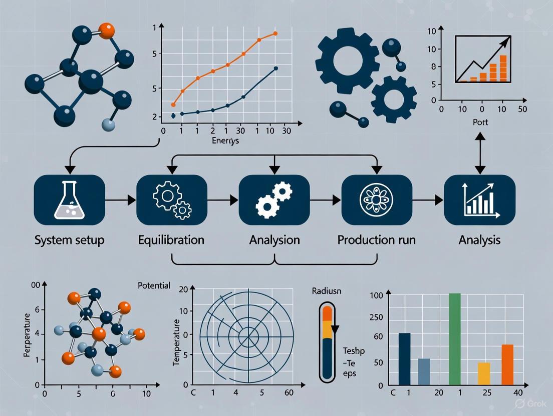
A complete MD simulation involves multiple stages that extend beyond the core integration algorithm. The typical workflow includes:
Initialization: The system is defined by initial positions (typically from experimental structures) and initial velocities (usually drawn from a Maxwell-Boltzmann distribution). The potential energy V arising from interatomic interactions is computed [2].
Force Computation: Forces on each atom are calculated as Fᵢ = -∂V/∂rᵢ. This is the most computationally intensive step, as it involves evaluating all bonded and non-bonded interactions in the system [2].
Integration: The Velocity Verlet algorithm propagates the system forward by one time step, updating positions and velocities.
Iteration: Steps 2-3 are repeated for the desired number of time steps, generating a trajectory of the system [2].
Analysis: The resulting trajectory is analyzed to extract physically meaningful properties, such as energies, structural changes, or dynamic correlations.
The Scientist's Toolkit: Essential Components for MD Simulations
Table 2: Essential Research Reagents and Computational Tools for Molecular Dynamics
| Component | Type | Function/Purpose | Examples |
|---|---|---|---|
| Integration Algorithms | Software Component | Numerically solve equations of motion | Velocity Verlet, Leapfrog [2] [4] |
| Force Fields | Parameter Set | Define potential energy functions | CHARMM, AMBER, OPLS [5] |
| Solvent Models | Parameter Set | Represent water and other solvents | TIP3P, SPC/E, implicit solvent [1] |
| Simulation Software | Application Platform | Implement MD algorithms and workflows | OpenMM, GROMACS, NAMD [5] [6] |
| Analysis Tools | Software Library | Process trajectories and compute properties | MDTraj, Crossflow [5] [7] |
| Enhanced Sampling | Advanced Method | Accelerate rare events | Metadynamics, Umbrella Sampling [8] |
Advanced Applications and Recent Developments
Specialized Applications of Velocity Verlet
The robustness of the Velocity Verlet algorithm has enabled its adaptation to specialized simulation scenarios. Researchers have developed modifications to handle strong external magnetic fields, where conventional techniques demand the simulation time step Δt be small compared to the Larmor oscillation time 2π/Ω. The modified Velocity Verlet approach builds the magnetic field directly into the propagation equations, making the choice of Δt independent of 2π/Ω and thus significantly improving efficiency for strongly magnetized systems [9]. Such specialized applications demonstrate the algorithm's flexibility and continued relevance across diverse physical scenarios.
Integration with Modern Computational Workflows
Contemporary research increasingly incorporates MD simulations into larger, automated workflows. Tools like Crossflow, a Python library built on Dask.distributed, enable researchers to construct complex computational workflows that integrate Velocity Verlet-based MD with other simulation and analysis tasks [7]. Similarly, MDCrow represents an LLM-based agentic system that can automate MD workflow setup and execution, including parameter selection, simulation running, and analysis [5]. These developments are making sophisticated MD simulations more accessible while maintaining the fundamental integration algorithms like Velocity Verlet at their core.
Emerging Trends and Future Directions
The field of molecular dynamics continues to evolve, with several emerging trends building upon foundational integration methods. Machine learning approaches are being integrated with MD simulations for enhanced analysis of complex trajectories [8]. Quantum mechanics/molecular mechanics (QM/MM) methods combine the accuracy of quantum chemistry with the efficiency of classical force fields, with Velocity Verlet often serving as the integration engine for the classical regions [8]. GPU-accelerated computing has dramatically expanded the accessible timescales of MD simulations, from nanoseconds in the 1990s to routine microsecond simulations today, all while relying on the same fundamental integration algorithms [8]. These advances ensure that the Velocity Verlet algorithm will remain a cornerstone of molecular simulation methodology for the foreseeable future.
In the molecular dynamics (MD) workflow for atomic trajectories research, the force field serves as the fundamental computational model that defines the potential energy of a system and governs the forces between atoms. The choice between an all-atom (AA) and a coarse-grained (CG) representation constitutes one of the most critical early decisions in any MD study, with profound implications for the balance between computational efficiency and atomistic detail. A force field consists of mathematical functions and parameters used to calculate the potential energy of a system at the atomistic level, typically including terms for both bonded interactions (bonds, angles, dihedrals) and nonbonded interactions (electrostatic and van der Waals forces) [10]. This technical guide provides researchers and drug development professionals with a comprehensive framework for selecting appropriate force field resolutions based on their specific research objectives, system characteristics, and computational resources.
Fundamental Concepts: Resolution Levels and Physical Basis
All-Atom, United-Atom, and Coarse-Grained Representations
Molecular dynamics force fields exist along a spectrum of resolution, with each level offering distinct advantages and limitations for simulating atomic trajectories:
All-Atom (AA) Force Fields: AA force fields explicitly represent every atom in the system, including hydrogen atoms. This approach provides the highest level of detail, making it suitable for studying phenomena where atomic-level interactions are critical, such as precise ligand binding, chemical reactions, or detailed conformational changes [11] [10]. The CHARMM36 and AMBER ff19SB are examples of widely used AA force fields in biomolecular simulations [12].
United-Atom (UA) Force Fields: UA force fields represent aliphatic hydrogens implicitly by grouping them with their parent carbon atoms, thereby reducing the total number of particles in the system. This offers a middle ground between computational efficiency and atomic detail [11].
Coarse-Grained (CG) Force Fields: CG force fields significantly simplify the molecular representation by grouping multiple atoms into single interaction centers or "beads." Popular CG force fields like MARTINI and SIRAH can improve computational efficiency by several orders of magnitude, enabling the simulation of larger systems and longer timescales [12] [13]. This reduction in detail smooths the energy landscape and reduces molecular friction, allowing faster exploration of conformational space [13].
Table 1: Comparison of Force Field Resolutions for Molecular Dynamics
| Feature | All-Atom (AA) | United-Atom (UA) | Coarse-Grained (CG) |
|---|---|---|---|
| Atomic Representation | Explicit representation of all atoms, including hydrogens | Aliphatic hydrogens grouped with carbon atoms | Multiple atoms grouped into single "beads" |
| Computational Cost | Highest | Moderate | Significantly reduced |
| Simulation Timescales | Nanoseconds to microseconds | Microseconds | Microseconds to milliseconds |
| Spatial Scales | Small to medium systems (up to ~1 million atoms) | Medium systems | Large systems (millions to billions of atoms) |
| Level of Detail | Atomic-level interactions | Atomic-level for heavy atoms, simplified for aliphatic groups | Mesoscopic, missing atomic details |
| Common Force Fields | CHARMM36, AMBER ff19SB, OPLS-AA | OPLS-UA, GROMOS | MARTINI, SIRAH, UNRES |
| Typical Applications | Ligand binding, detailed conformational changes, reaction mechanisms | Membrane systems, lipid bilayers | Large macromolecular complexes, cellular components |
Mathematical Foundations of Force Fields
The basic functional form of the potential energy in most molecular mechanics force fields follows a consistent pattern, though the specific implementation varies between different force fields. The total energy is typically decomposed into bonded and nonbonded components [10]:
[ E{\text{total}} = E{\text{bonded}} + E_{\text{nonbonded}} ]
Where the bonded terms are further decomposed as: [ E{\text{bonded}} = E{\text{bond}} + E{\text{angle}} + E{\text{dihedral}} ] And the nonbonded terms include: [ E{\text{nonbonded}} = E{\text{electrostatic}} + E_{\text{van der Waals}} ]
The bond stretching energy is typically modeled using a harmonic potential approximating Hooke's law: [ E{\text{bond}} = \frac{k{ij}}{2}(l{ij} - l{0,ij})^2 ] where ( k{ij} ) is the bond force constant, ( l{ij} ) is the actual bond length, and ( l_{0,ij} ) is the equilibrium bond length [10].
Electrostatic interactions are generally represented by Coulomb's law: [ E{\text{Coulomb}} = \frac{1}{4\pi\varepsilon0}\frac{qi qj}{r{ij}} ] where ( qi ) and ( qj ) are the atomic charges, ( r{ij} ) is the distance between atoms, and ( \varepsilon_0 ) is the vacuum permittivity [10].
Practical Selection Framework: Choosing the Appropriate Resolution
Systematic Decision Criteria for Force Field Selection
Selecting the appropriate force field resolution requires careful consideration of multiple scientific and practical factors. The following workflow provides a structured approach to this decision process:
The selection of force field resolution directly impacts the physical accuracy and computational feasibility of MD simulations. The following table summarizes key performance characteristics and limitations of each approach:
Table 2: Performance Characteristics and Limitations of Different Force Field Resolutions
| Aspect | All-Atom (AA) | Coarse-Grained (CG) |
|---|---|---|
| Accuracy of Atomic Interactions | High - captures detailed atomic interactions and stereochemistry | Limited - loses atomic details, may miss specific interactions |
| Computational Efficiency | Lower - requires significant computational resources for meaningful simulations | Higher - enables simulation of larger systems and longer timescales |
| Sampling Efficiency | Slower - rugged energy landscape with high barriers | Faster - smoothed energy landscape with reduced friction [13] |
| Representation of Energetics | Direct - based on physical principles with some empirical parameterization | Indirect - often based on statistical potentials from databases [12] |
| Handling of Polarization Effects | Explicit - through polarizable force fields or fixed-charge approximations with scaling | Implicit - through effective parameters, with recent advances in polarizable CG models [13] |
| Transferability | Generally good for related systems, but requires careful validation | Can be limited, especially for systems not well-represented in training data [12] |
| Physical Interpretation | More straightforward connection to physical chemistry principles | Requires mapping back to atomic details for full interpretation |
Case Studies and Empirical Comparisons
Real-world comparisons between AA and CG simulations reveal practical performance differences that inform selection decisions. In a study comparing AA (CHARMM36) and CG (MARTINI) simulations of a POPC lipid bilayer under equibiaxial stretching, the CG system exhibited approximately half the von Mises stress values of the AA system despite identical simulation conditions [14]. This discrepancy was attributed to reduced friction and fewer entropic contributions in the CG representation, where multiple atoms are collapsed into single beads, particularly during non-equilibrium processes like deformation [14].
For intrinsically disordered proteins (IDPs) like amyloid-β, both AA and CG approaches can provide reasonable results, but CG methods may lack certain atomistic details, such as precise secondary structure recognition, due to the inherent simplifications in the model [12]. Recent improvements in CG force fields, particularly adjustments to protein-water interaction scaling in MARTINI, have enhanced their ability to capture IDP behavior more accurately [12].
Methodological Protocols: Implementation Guidelines
Standard Simulation Workflow for AA and CG Simulations
The following diagram illustrates the general MD workflow, highlighting key differences between AA and CG approaches:
Detailed Experimental Protocols
All-Atom Simulation Protocol for Intrinsically Disordered Proteins
Based on established methodologies for studying systems like amyloid-β [12]:
System Setup
- Obtain initial protein structure from experimental data or homology modeling
- Solvate the protein in an appropriate water model (OPC recommended for IDPs with AMBER ff19SB)
- Add ions to neutralize the system and achieve desired physiological concentration
Energy Minimization
- Apply steepest descent algorithm for 5,000-10,000 steps
- Use position restraints on protein heavy atoms (force constant: 1000 kJ/mol/nm²)
- Confirm significant reduction in potential energy and maximum force < 1000 kJ/mol/nm
Equilibration
- NVT equilibration for 100-500 ps with protein heavy atoms restrained
- Maintain temperature at 310 K using modified Berendsen thermostat
- NPT equilibration for 1-5 ns with protein heavy atoms restrained
- Maintain pressure at 1 bar using Parrinello-Rahman barostat
- Gradually release position restraints on protein backbone and side chains
Production Simulation
- Run multiple independent trajectories (3-5) of 100 ns - 1 µs each
- Use a 2-fs time step with bonds constrained to hydrogen atoms using LINCS
- Employ replica exchange molecular dynamics if enhanced sampling is required
Coarse-Grained Simulation Protocol Using MARTINI
System Preparation
- Convert atomistic structure to CG representation using appropriate mapping
- For proteins, use the martinize.py script with Elnedyn elastic network
- Solvate the system with standard MARTINI water molecules
- Add ions as needed for neutralization
Energy Minimization
- Perform steepest descent minimization for 1,000-5,000 steps
- No position restraints typically required for CG systems
Equilibration
- NVT equilibration for 10-100 ns with protein backbone restraints (force constant: 1000 kJ/mol/nm²)
- Maintain temperature using velocity rescale thermostat
- NPT equilibration for 50-200 ns with protein backbone restraints
- Maintain pressure at 1 bar using Parrinello-Rahman barostat
- Gradually release restraints in 2-3 stages
Production Simulation
- Run production for 1-10 µs depending on system size and processes of interest
- Use 10-20 fs time step
- For IDPs, apply protein-water interaction scaling (0.85-0.95) to prevent over-compaction
Table 3: Essential Tools and Resources for Molecular Dynamics Simulations
| Tool Category | Specific Tools/Software | Primary Function | Key Features |
|---|---|---|---|
| Simulation Packages | GROMACS [14] [12], AMBER [12] | Molecular dynamics engine | High performance, extensive force field support |
| Visualization Software | VMD, ChimeraX [15] | Trajectory analysis and visualization | Multiple representation styles, scripting capability |
| Force Field Databases | MolMod [10], TraPPE [10] | Force field parameter repositories | Curated parameters for specific molecular classes |
| Analysis Tools | MDTraj, MDAnalysis | Trajectory analysis | Python-based, programmable analysis workflows |
| Specialized CG Tools | MARTINI [12] [13], SIRAH [12] | Coarse-grained force fields | Balanced detail and efficiency for large systems |
| Validation Resources | PDB, NMR data [12] | Simulation validation | Experimental reference data for force field testing |
Emerging Trends and Future Directions
The field of molecular dynamics continues to evolve with several emerging trends that impact force field selection and application. Machine learning approaches are increasingly being applied to both force field development and surrogate modeling of MD trajectories [13] [16]. Generative models of molecular trajectories, such as MDGen, represent a promising approach for learning flexible multi-task surrogate models from MD data, enabling applications in forward simulation, transition path sampling, trajectory upsampling, and dynamics-conditioned molecular design [16].
Polarizable force fields constitute another significant advancement, addressing the critical limitation of fixed-charge models in handling electronic polarization effects [13]. For CG models, recent developments include polarizable variants using Drude oscillators and QM-based polarizable models that more accurately capture the electrostatic environments in complex systems like ionic liquids [13].
Multi-scale modeling approaches that seamlessly integrate different resolutions are also gaining traction, allowing researchers to apply high-resolution AA models to critical regions while using efficient CG representations for less critical parts of the system. These advancements are progressively blurring the traditional boundaries between AA and CG approaches, offering researchers more nuanced options for balancing computational efficiency with physical accuracy.
As the field advances toward simulating increasingly complex systems, including entire cellular environments [15], the judicious selection and application of appropriate force fields will remain fundamental to generating physically meaningful atomic trajectories and extracting biologically significant insights from molecular dynamics simulations.
In molecular dynamics (MD) research, the initial system setup is a critical determinant of simulation reliability and accuracy. This phase transforms a static molecular structure into a dynamic model that approximates realistic experimental or physiological conditions. Proper configuration of the simulation box, solvation environment, and ion concentration establishes the physical context for atomic trajectory research, directly influencing the thermodynamic and kinetic properties extracted from simulations [17] [18]. For researchers and drug development professionals, rigorous implementation of these foundational steps ensures that subsequent trajectory analysis provides meaningful insights into molecular behavior, binding interactions, and dynamic processes relevant to therapeutic design.
The simulation setup process bridges the gap between isolated molecular structures and their behavior in complex environments. As MD simulations track the movement of individual atoms and molecules over time by numerically solving Newton's equations of motion, they offer a unique window into atomic-scale processes that are often difficult or impossible to observe experimentally [17] [19]. The accuracy of this "computational microscope" depends fundamentally on how well the simulated system represents reality, making initial setup decisions critical for generating physically meaningful trajectories.
Defining the Simulation Box and Boundary Conditions
Simulation Box Fundamentals
The simulation box defines the spatial domain containing all particles to be simulated. This finite volume must be carefully constructed to balance computational efficiency with physical accuracy, as its dimensions directly determine the number of atoms in the system and consequently the computational resources required [20]. The primary challenge lies in simulating biologically or materials-relevant behavior with a tractable number of atoms, typically thousands to millions rather than the Avogadro-scale numbers found in macroscopic systems [19].
The selection of box shape represents a critical early decision with significant implications for sampling efficiency. While a simple cubic box may be most intuitive, other geometries often provide better performance for biomolecular simulations [20].
Table 1: Common Simulation Box Geometries and Their Applications
| Box Type | Mathematical Definition | Primary Advantages | Typical Applications |
|---|---|---|---|
| Cubic/Orthorhombic | Three equal or unequal edge lengths at 90° angles | Simple implementation; intuitive | General purpose; crystalline materials |
| Rhombic Dodecahedron | Twelve identical rhombic faces | Most efficient for spherical molecules; minimal volume | Globular proteins; micellar simulations |
| Truncated Octahedron | Eight hexagonal and six square faces | Good balance of efficiency and simplicity | Solvated proteins; nucleic acids |
| Hexagonal Prism | Two hexagonal bases with rectangular sides | Suitable for elongated molecules | DNA; filamentous proteins |
Periodic Boundary Conditions
Periodic Boundary Conditions (PBCs) represent the most widely adopted solution to the surface artifact problem inherent to finite simulation volumes. Rather than simulating an isolated cluster of atoms with artificial surfaces, PBCs create an infinite periodic system by tiling space with identical copies of the primary simulation cell [20]. Under this framework, each atom in the primary cell interacts not only with other atoms in the same cell but also with their periodic images in adjacent cells.
The mathematical implementation of PBCs treats particle coordinates as modular with respect to box dimensions. For a particle at position r = (x, y, z) in a cubic box of side length L, its periodic images appear at positions r + (iL, jL, kL) for all integer combinations of i, j, k [20]. When a particle exits the primary box through one face, it simultaneously re-enters from the opposite face, maintaining a constant number of particles throughout the simulation [20].
The minimum image convention governs interatomic interactions within PBCs, specifying that each atom interacts only with the single closest copy of every other atom (either the original or one of its images) [20]. This convention requires that the box dimensions exceed twice the non-bonded interaction cutoff distance (L > 2r_cut) to prevent atoms from interacting with multiple copies of the same particle. For typical biomolecular simulations with cutoff distances of 1.0-1.2 nm, this necessitates box sizes of at least 2.0-2.4 nm in each dimension [20].
Solvation: Creating the Aqueous Environment
Explicit vs. Implicit Solvent Models
Solvation refers to the process of surrounding solute molecules (proteins, nucleic acids, drug compounds) with solvent molecules to create a realistic environmental context. The choice between explicit and implicit solvent representations represents a fundamental trade-off between computational efficiency and physical accuracy [19].
Table 2: Comparison of Explicit and Implicit Solvation Methods
| Parameter | Explicit Solvent | Implicit Solvent |
|---|---|---|
| Representation | Individual solvent molecules (e.g., ~3 atoms for TIP3P water) | Continuum dielectric medium |
| Computational Cost | High (thousands of additional atoms) | Low (no additional atoms) |
| Accuracy for | Hydrogen bonding, specific hydration, diffusion | Thermodynamic properties, rapid screening |
| Common Models | TIP3P, TIP4P, SPC, OPC [21] [22] | Generalized Born (GB), Poisson-Boltzmann (PB) |
| Implementation | Solvent molecules added to simulation box | Dielectric constant assigned to extra-molecular space |
Explicit solvent models provide atomic detail of solute-solvent interactions at the expense of significantly increased system size and computational requirements. For a typical globular protein, water molecules can constitute 80-90% of the total atoms in the system [19]. Implicit solvent (continuum) models approximate the solvent as a dielectric medium characterized by a dielectric constant, dramatically reducing system complexity while potentially sacrificing specific interaction details [23] [19].
Practical Solvation Methodology
The technical process of solvation begins with placing the solute molecule in an appropriately sized simulation box, followed by insertion of solvent molecules into all regions not occupied by the solute. The solvatebox command in tools like tLEaP (AMBER) or solvation utilities in GROMACS automatically fill the available volume with solvent molecules arranged in pre-equilibrated configurations [21].
A critical consideration is ensuring sufficient solvent padding between the solute and box boundaries. For proteins, a minimum distance of 1.0-1.5 nm between any protein atom and the box edge is generally recommended to prevent artificial correlations between periodic images [21] [22]. This padding ensures that the solute does not interact with its own periodic images across the box boundaries, which would create unphysical constraints on conformational dynamics.
The following workflow diagram illustrates the sequential steps in system solvation:
Adding Ions: Neutralization and Physiological Conditions
Purpose of Ion Addition
The introduction of ions into the simulation system serves two primary purposes: neutralizing the overall system charge and establishing physiologically relevant salt concentrations. Most biomolecules carry substantial net charges under physiological conditions - for example, lysozyme possesses a charge of +8 [22]. Without counterions, these charged systems would generate unrealistic electrostatic interactions under periodic boundary conditions, leading to unphysical dynamics and artifacts in atomic trajectories [21].
Beyond neutralization, the addition of salt ions at appropriate concentrations mimics the physiological or experimental environment being modeled. Ionic composition affects conformational sampling, dynamics, and function of biological macromolecules through screening of electrostatic interactions and specific ion binding effects [21]. For simulations targeting biological relevance, 150 mM NaCl approximates physiological salt concentration, though specialized contexts may require different ionic compositions or concentrations [21].
Ion Placement Methods
Two principal methodologies exist for introducing ions into solvated systems: random placement and electrostatic potential-guided placement. Random placement substitutes randomly selected solvent molecules with ions, while potential-guided placement positions ions at points of favorable electrostatic potential relative to the solute [21].
The number of ions required for neutralization depends directly on the net charge of the solute macromolecule. For a system with net charge +Q, exactly Q counterions (typically Cl⁻ for positively charged solutes) must be added to achieve neutrality [21] [22]. To establish specific salt concentrations beyond neutralization, the number of additional ion pairs follows the formula:
Nions = 0.0187 × [Molarity] × Nwater
where N_water represents the number of water molecules in the system, and [Molarity] is the target salt concentration [21]. For increased accuracy, computational servers like SLTCAP can calculate ion numbers corrected for screening effects, which may yield slightly different values than this empirical formula [21].
Table 3: Ion Types and Properties in Common Force Fields
| Ion Type | Common Force Field Parameters | Hydration Properties | Typical Applications |
|---|---|---|---|
| Na⁺ | CHARMM, AMBER, OPLS variants | Strong first hydration shell; low diffusion | Physiological mimicry; nucleic acid systems |
| K⁺ | CHARMM, AMBER, OPLS variants | Weaker hydration; higher diffusion | Intracellular environments; ion channels |
| Cl⁻ | CHARMM, AMBER, OPLS variants | Moderate hydration; anion interactions | General counterion; charge neutralization |
| Ca²⁺ | Specialized parameters | Strong coordination; slow exchange | Signaling systems; metalloproteins |
| Mg²⁺ | Specialized parameters | Tight hydration; high charge density | Nucleic acid folding; ATP-dependent enzymes |
The following workflow illustrates the ion addition process:
Integrated Workflow: From Structure to Solvated System
Complete Setup Procedure
Implementing a robust system setup requires sequential execution of the aforementioned steps, typically facilitated by MD preparation tools such as tLEaP (AMBER), GROMACS utilities, or CHARMM scripting. The following integrated protocol details a complete workflow from initial structure to solvated, ionized system ready for energy minimization:
Initial Structure Preparation: Obtain atomic coordinates from databases such as the Protein Data Bank (PDB) or Materials Project. Process the structure to remove heteroatoms, add missing residues or atoms, and assign protonation states appropriate for the target pH [22] [24].
Force Field Selection: Choose an appropriate force field (e.g., AMBER, CHARMM, OPLS-AA) and water model consistent with the research objectives and compatible with the solute molecule [22] [18]. Apply force field parameters to generate molecular topology.
Simulation Box Definition: Center the solute in an appropriately sized box with geometry selected based on molecular shape. Ensure minimum distance of 1.0-1.5 nm between solute and all box boundaries [20] [22].
System Solvation: Fill the simulation box with water molecules using the selected water model. For explicit solvent simulations, this typically employs pre-equilibrated water configurations that are merged with the solute structure [21] [22].
Ion Addition: First, add sufficient counterions to neutralize the system net charge. Subsequently, add additional ion pairs to achieve the target physiological or experimental salt concentration [21] [25].
System Validation: Verify final system composition, check for atomic overlaps, and confirm appropriate charge distribution before proceeding to energy minimization.
The following diagram provides a comprehensive overview of the complete system setup workflow:
Table 4: Essential Software Tools and Databases for MD System Setup
| Tool Category | Specific Tools/Resources | Primary Function | Access/Reference |
|---|---|---|---|
| Structure Databases | Protein Data Bank (PDB); Materials Project; PubChem | Source experimental structures | https://www.rcsb.org/; https://materialsproject.org/ |
| Force Fields | AMBER (ff19SB); CHARMM36; OPLS-AA; GROMOS | Molecular mechanics parameters | [22] [24] |
| Setup Utilities | tLEaP (AMBER); pdb2gmx (GROMACS); CHARMM-GUI | Topology generation; system building | [21] [22] |
| Solvation Tools | Solvate tool (GROMACS); Solvate plugin (VMD) | Add explicit solvent molecules | [21] [22] |
| Ion Placement | Autoionize (VMD); genion (GROMACS); SLTCAP server | Add ions for neutralization/salt concentration | [21] [25] |
| Validation Tools | VMD; ChimeraX; GROMAC energy analysis | Visual inspection; energy sanity checks | [24] [18] |
The meticulous setup of simulation boxes, solvation environments, and ion distributions establishes the physical basis for meaningful molecular dynamics trajectories. These initial conditions directly control the quality and biological relevance of the dynamic behavior observed in atomic-level simulations. For research aimed at understanding molecular mechanisms or supporting drug development initiatives, rigorous implementation of these foundational steps aligns simulation outcomes with experimental observables, creating a robust platform for extracting scientifically valid insights from atomic trajectories. As MD simulations continue to bridge theoretical and experimental approaches in molecular science, standardized, well-documented system preparation remains indispensable for generating reproducible, physically-grounded computational results.
Within the broader molecular dynamics (MD) workflow for atomic trajectories research, the establishment of stable initial conditions is a critical prerequisite for obtaining physically meaningful and reproducible simulation data. This guide details the core protocols for energy minimization and system equilibration, two foundational steps that ensure a simulation starts from a stable, low-energy configuration. Proper execution of these steps mitigates instabilities caused by unphysical atomic overlaps, incorrect bond geometries, or high internal stresses, which could otherwise lead to simulation failure or inaccurate results. For researchers, scientists, and drug development professionals, a rigorous approach to these initial phases is indispensable for the reliability of subsequent trajectory analysis.
Energy Minimization: Core Algorithms and Protocols
Energy minimization (EM), also known as energy optimization, is the process of iteratively adjusting atomic coordinates to find a local minimum on the potential energy surface. This step resolves steric clashes and unphysical conformations that may exist in the initial structure, often resulting from model building or experimental structure limitations.
Three common algorithms for energy minimization are the steepest descent, conjugate gradient, and L-BFGS methods [26]. The choice of algorithm involves a trade-off between robustness, computational efficiency, and the specific requirements of the system.
Steepest Descent: This robust algorithm is highly effective in the initial stages of minimization when the system is far from an energy minimum. It moves atomic coordinates in the direction of the negative energy gradient (the force). Although not the most efficient, it is very stable for poorly conditioned systems. The maximum displacement is dynamically adjusted based on whether a step decreases the potential energy; it is increased by 20% for successful steps and reduced by 80% for rejected steps [26].
Conjugate Gradient: This algorithm is more efficient than steepest descent as it approaches the energy minimum but can be less robust in the early stages. It uses information from previous steps to choose conjugate descent directions, leading to faster convergence near the minimum. A key limitation is that it cannot be used with constraints, meaning flexible water models are required if water is present [26].
L-BFGS (Limited-memory Broyden–Fletcher–Goldfarb–Shanno): A quasi-Newtonian method, L-BFGS builds an approximation of the inverse Hessian matrix (the matrix of second derivatives) to achieve faster convergence. It typically converges faster than conjugate gradients but is not yet parallelized in all MD software packages due to its reliance on correction steps from previous iterations [26].
Table 1: Comparison of Energy Minimization Algorithms in GROMACS
| Algorithm | Strengths | Weaknesses | Recommended Use Case |
|---|---|---|---|
| Steepest Descent | Robust, easy to implement, effective with large forces | Slow convergence near minimum | Initial minimization of poorly conditioned systems |
| Conjugate Gradient | More efficient closer to minimum | Less robust initially; cannot be used with constraints | Subsequent minimization after initial steepest descent |
| L-BFGS | Fastest convergence | Not yet fully parallelized in some software | Minimization of well-conditioned systems where speed is critical |
Practical Implementation and Stopping Criteria
A common and effective strategy is to use a hybrid approach, initiating minimization with the steepest descent algorithm and then switching to conjugate gradient or L-BFGS for final convergence. A real-world protocol for a solvated glycoprotein system, for instance, involved 10,000 steps of steepest descent followed by 10,000 steps of conjugate gradient [27].
The minimization process is typically stopped when the maximum force components in the system fall below a specified threshold, ε. An overly tight criterion can lead to endless iterations due to numerical noise. A reasonable value for ε can be estimated from the root-mean-square force of a harmonic oscillator at a given temperature. For a weak oscillator, this value is on the order of 1-10 kJ mol⁻¹ nm⁻¹, which provides an acceptable stopping criterion [26].
System Equilibration: Achieving Thermodynamic Equilibrium
Following energy minimization, the system must be equilibrated to bring it to the target temperature and pressure, allowing the solvent to relax around the solute and the system to adopt a representative configuration for the desired thermodynamic ensemble.
A Phased Equilibration Protocol
Equilibration is often performed in stages, gradually releasing positional restraints on the solute to prevent large structural distortions as the solvent environment stabilizes. A detailed protocol from a large-scale MD dataset (mdCATH) illustrates this process [28]:
- Restrained Equilibration: The system is equilibrated for 10 ns in the NPT ensemble (constant Number of particles, Pressure, and Temperature). During this phase, harmonic restraints are applied to the protein's Cα atoms (with a force constant of 1.0 kcal/mol/Ų) and all heavy atoms (0.1 kcal/mol/Ų) to maintain the protein's native structure.
- Unrestrained Equilibration: The restraints are removed, and the system is equilibrated for a further 10 ns in the NPT ensemble. This allows the entire system to fully relax.
Another protocol for a glycosylated system involved a 400 ps equilibration at 300 K with restraints on solute heavy atoms, followed by a 1 ns equilibration with restraints only on the Cα atoms before initiating production simulations [27].
Ensemble and Thermostat/Barostat Selection
The choice of thermodynamic ensemble and regulation methods is critical. The mdCATH dataset performed production runs in the NVT (constant Number of particles, Volume, and Temperature) ensemble to avoid issues with the poor reproduction of the water phase diagram by the TIP3P water model [28]. For temperature coupling, the Langevin thermostat (with a collision frequency of 2 ps⁻¹ in one study [27] and 0.1 ps⁻¹ in another [28]) and the Berendsen thermostat (with a very short time constant in automated workflows [29]) are commonly used, especially during equilibration. For pressure coupling, the Berendsen barostat is often used during equilibration due to its robustness, as in the protocol that used a 1 ps time constant [27].
Table 2: Example Equilibration and Production Parameters from Published Protocols
| Parameter | Protocol A (Glycoprotein) [27] | Protocol B (mdCATH Dataset) [28] |
|---|---|---|
| Force Field | AMBER14SB & GLYCAM06j | CHARMM22* |
| Water Model | TIP3P | TIP3P |
| Electrostatics | Particle Mesh Ewald (PME) | Particle Mesh Ewald (PME) |
| Equilibration Ensemble | NPT | NPT |
| Thermostat | Langevin (2 ps⁻¹) | Langevin (0.1 ps⁻¹) |
| Barostat | Berendsen (1 ps) | Monte Carlo |
| Positional Restraints | Heavy atoms, then Cα only | Cα and heavy atoms, then none |
| Production Ensemble | NPT | NVT |
Integrated Workflows and Visualization
The energy minimization and equilibration steps are integral parts of a larger, automated MD workflow. These steps are often embedded within larger simulation paradigms, such as active learning for machine learning potentials, where an initial structure is prepared, its energy is minimized, and it is equilibrated before active learning production cycles begin [30]. Specialized MD workflows also implement automated "first-aid" functions to rescue simulations that fail, which can include re-invoking minimization and equilibration protocols [31].
The following diagram outlines the logical progression from initial system construction to a production-ready simulation, highlighting the decision points within the energy minimization and equilibration phases.
The Scientist's Toolkit: Essential Reagents and Software
Successful execution of energy minimization and equilibration protocols relies on a suite of software tools and "research reagents," which include force fields, solvent models, and analysis utilities.
Table 3: Essential Research Reagent Solutions for MD Preparation
| Category | Item | Function/Brief Explanation |
|---|---|---|
| MD Engines | GROMACS [26], AMBER [27], OpenMM (via drMD) [31], LAMMPS [32] | Software that performs the numerical integration of the equations of motion for energy minimization and dynamics. |
| Force Fields | CHARMM22* [28], AMBER14SB [27], GLYCAM06j [27], Martini [33] | Empirical potential functions defining bonded and non-bonded interactions between atoms. Critical for energy evaluation. |
| Solvent Models | TIP3P [27] [28] | A common 3-site water model used to solvate the system during the building phase. |
| Analysis & Visualization | VMD [32], Travis [32], HTMD [28] | Tools for visualizing trajectories, calculating properties like RMSD/RMSF, and checking the stability of equilibration. |
| System Building | PACKMOL [32], drMD [31] | Tools for creating initial simulation boxes by packing molecules (e.g., solute, water, ions) into a defined volume. |
Energy minimization and equilibration are not merely procedural formalities but are scientifically critical steps for ensuring the stability and physical validity of molecular dynamics simulations. By understanding the algorithms, implementing phased protocols with appropriate restraints and thermodynamic controls, and utilizing the available software tools effectively, researchers can generate reliable initial conditions. This rigorous approach lays the necessary foundation for obtaining accurate atomic trajectories, which is paramount for subsequent analysis in fields ranging from fundamental biophysics to computer-aided drug design.
This technical guide details the critical parameters for the production phase of a Molecular Dynamics (MD) simulation, framed within the broader thesis of understanding the MD workflow for atomic trajectories research. The production run is the final stage where a physically sound trajectory is generated for subsequent analysis, making the correct configuration of time step, total steps, and ensemble controls paramount for obtaining reliable, publishable results. This document provides in-depth methodologies and structured data to guide researchers and drug development professionals in optimizing these core parameters.
The molecular dynamics workflow is a multi-stage process that progresses from system preparation and energy minimization through equilibration, culminating in the production run [22]. While equilibration stabilizes the system's temperature and pressure, the production simulation is where the actual trajectory used for data analysis is generated [34]. The parameters chosen for this phase directly control the physical accuracy, numerical stability, and statistical significance of the simulation. A well-configured production run samples the correct thermodynamic ensemble, conserves energy (or its extended equivalent), and avoids numerical artifacts, thereby providing a trustworthy foundation for analyzing atomic trajectories.
The Integration Time Step
The integration time step (dt) is the most fundamental numerical parameter, determining the interval at which Newton's equations of motion are solved. An excessively small dt leads to unrealistically long simulation times for a given number of steps, while an overly large dt causes instability and energy drift, potentially crashing the simulation [35].
Theoretical Foundation: The Nyquist Criterion and Fastest Vibrations
The upper limit for the time step is governed by the Nyquist sampling theorem, which states that the time step must be half or less of the period of the quickest dynamics in the system [35]. In practice, a more conservative ratio of 0.01 to 0.033 of the shortest vibrational period is recommended for accurate integration [35]. The highest-frequency motions in biomolecular systems are typically bond vibrations involving hydrogen atoms (e.g., C-H bonds with a period of ~11 femtoseconds), which would theoretically permit a time step of about 5 fs [35]. However, standard practice often uses a 2 fs time step when bonds involving hydrogens are constrained, providing a good balance between accuracy and efficiency [35].
Practical Validation: Monitoring Energy Conservation
Theoretical rules of thumb must be validated empirically. The most robust method for assessing time step appropriateness is to monitor the drift in the conserved quantity (e.g., total energy in an NVE ensemble) over a short simulation [35]. A reasonable rule of thumb is that the long-term drift should be less than 1 meV/atom/ps for publishable results, and can be up to 10 meV/atom/ps for qualitative work [35]. A significant drift indicates that the time step is too large or the integrator is not behaving time-reversibly.
Table 1: Guidelines for Time Step Selection
| System / Condition | Recommended Time Step (fs) | Key Considerations |
|---|---|---|
| Standard atomistic (with H-bonds constrained) | 2 | Default for most biomolecular simulations with constraints [35] |
| Systems with light nuclei (H) | 0.25 - 1 | Necessary for accurate hydrogen dynamics [35] |
| Using mass repartitioning | 3 - 4 | Mass of light atoms is scaled up, allowing a larger dt [36] |
| Target energy drift (publishable) | Configure to achieve < 1 meV/atom/ps | Must be checked in an NVE simulation [35] |
| Target energy drift (qualitative) | Configure to achieve < 10 meV/atom/ps | Must be checked in an NVE simulation [35] |
The following workflow diagram outlines the process of selecting and validating a time step:
Total Simulation Steps and Time
The nsteps parameter determines the total number of integration steps and, when multiplied by the time step (dt), defines the total simulated time. The choice of nsteps is dictated by the scientific question, specifically the timescales of the processes under investigation [18].
Connecting Steps to Physical Time and Phenomena
The required simulation time can range from nanoseconds for local side-chain motions to microseconds or milliseconds for large conformational changes and protein folding [18]. It is critical to ensure that the total simulated time is long enough to sample the relevant biological process multiple times to obtain statistically meaningful results. For instance, a 1 ns simulation requires nsteps = 500,000 when using a 2 fs time step.
Thermostat and Barostat Controls
Thermostats and barostats are algorithms that maintain the temperature and pressure of the system, respectively, mimicking experimental conditions. Their proper configuration is essential for sampling the correct thermodynamic ensemble (e.g., NPT or NVT).
Thermostat Parameters
Thermostats maintain temperature by scaling particle velocities. Key parameters include the reference temperature (ref-t or temperature) and the coupling time constant (tau-t).
Table 2: Common Thermostat Algorithms and Parameters
| Thermostat | Algorithm Type | Key Parameters | Typical tau-t Value |
Notes |
|---|---|---|---|---|
| Nose-Hoover [37] | Deterministic | tau-t |
0.5 - 1.0 ps | Produces a correct canonical ensemble; often preferred for production. |
| Berendsen [37] | Stochastic | tau-t |
0.1 - 0.5 ps | Strongly damped; good for equilibration but not production [37]. |
| Velocity Rescale | Stochastic | tau-t |
0.1 - 0.5 ps | Corrects Berendsen's flaws; suitable for production. |
| Langevin [36] | Stochastic | tau-t (inverse friction) |
~2 ps [36] | Good for production; tau-t of 2 ps provides lower friction than water's internal friction [36]. |
Barostat Parameters
Barostats control the system pressure by adjusting the simulation box size. The choice of barostat must be consistent with the thermostat to achieve the desired ensemble.
Table 3: Common Barostat Algorithms and Parameters
| Barostat | Algorithm Type | Key Parameters | Typical tau-p Value |
Notes |
|---|---|---|---|---|
| Parrinello-Rahman | Deterministic | tau-p, compressibility |
1.0 - 5.0 ps | Produces a correct isobaric ensemble; often preferred for production. |
| Berendsen [37] | Stochastic | tau-p, compressibility |
0.5 - 1.0 ps | Strongly damped; good for equilibration but can produce an incorrect ensemble in production [37]. |
| MTK (Martyna-Tobias-Klein) | Deterministic | tau-p, compressibility |
1.0 - 5.0 ps | Extension of Nose-Hoover for pressure; used with Nose-Hoover thermostat for correct NPT ensemble. |
The relationship between these controls and the resulting thermodynamic ensemble is summarized below:
The Scientist's Toolkit: Essential Research Reagents and Software
This table details key software tools and "reagents" essential for conducting and analyzing MD production runs.
Table 4: Essential Software Tools for MD Production and Analysis
| Tool / Reagent | Type / Function | Relevance to Production Runs |
|---|---|---|
| GROMACS [38] [22] | MD Simulation Engine | High-performance, open-source software for running production simulations; implements all discussed parameters and algorithms. |
| MDP File [36] | Parameter Input File | A plain-text file that contains all parameters (e.g., dt, nsteps, thermostat settings) for a GROMACS simulation [36]. |
| MDTraj [39] | Trajectory Analysis Library | A modern, fast Python library for analyzing production trajectories (e.g., calculating RMSD, Rgyr). |
| TrajMap.py [40] | Trajectory Visualization Tool | A Python script for creating trajectory maps—2D heatmaps that visualize backbone movements over time. |
| PLUMED | Enhanced Sampling Plugin | A library for adding advanced sampling methods to production runs, often necessary for simulating rare events. |
Integrated Protocol for a Production MD Run
This protocol outlines the steps for configuring and launching a production run using common MD software like GROMACS, based on the parameters detailed above.
- Prepare the Equilibrated System: Use the final coordinates and topology from the successful NPT equilibration step as the input for the production run [34].
- Configure the MDP Parameters:
- Integrator: Set
integrator = md(leap-frog) orintegrator = md-vv(velocity Verlet) [36]. - Time Step: Define
dt = 0.002for a 2 fs time step [35]. - Total Steps: Set
nsteps = 500000for a 1 ns simulation. Adjust based on the timescale of your process of interest [18]. - Thermostat: Enable with
pcoupl = nofor NVT or use a thermostat like Nose-Hoover (tcoupl = Nose-Hoover) with atau-t = 1.0and the desiredref-t[36] [37]. - Barostat: For NPT ensembles, use a barostat like Parrinello-Rahman (
pcoupl = Parrinello-Rahman) with atau-p = 5.0and the correctcompressibilityfor your solvent [37].
- Integrator: Set
- Run the Simulation: Execute the production simulation using the MD engine. For large systems, this is typically done on a high-performance computing cluster.
- Validate the Output:
- Check Log Files: Monitor the potential energy, temperature, and pressure for stability.
- Verify Conservation (NVE): If an NVE test was run, confirm the energy drift is within acceptable limits (< 1 meV/atom/ps) [35].
- Analyze the Trajectory: Use analysis tools like MDTraj [39] to compute properties such as Root Mean Square Deviation (RMSD) and Radius of Gyration (Rgyr) from the production trajectory [34] [40].
Advanced MD Techniques and Their Applications in Drug Discovery and Diagnostics
Molecular Dynamics (MD) simulation serves as a computational microscope, enabling researchers to observe and quantify atomic-scale motions that govern biological and chemical processes. However, conventional MD faces fundamental limitations in capturing rare events—transitions between stable states separated by high energy barriers—due to the femtosecond time steps required for numerical integration, which collectively restrict simulations to microsecond or millisecond timescales at best. Many processes of biological and chemical significance, including protein folding, ligand binding, and chemical reactions, occur on timescales ranging from milliseconds to hours, creating a formidable sampling gap [41].
Enhanced sampling methods have emerged to bridge this timescale divide, employing sophisticated algorithms to accelerate the exploration of configurational space. These methods can be broadly categorized into several strategic families: those that apply bias potentials in collective variable space (such as Umbrella Sampling and Metadynamics), approaches utilizing generalized ensembles or replica exchange, and path-sampling techniques [41]. The focus of this technical guide is on two foundational methods in the first category: Umbrella Sampling (US) and Metadynamics (MTD), which have become essential tools for simulating rare events and calculating free energy landscapes across diverse scientific domains from drug discovery to materials science [42] [43].
At the core of these methods lies the concept of the collective variable (CV)—a low-dimensional representation of the system's slow degrees of freedom that typically captures the essential physics of the transition process. Proper selection of CVs is critical for the success of any enhanced sampling simulation, as inadequate CVs may fail to distinguish between relevant states or miss important transition pathways entirely [43]. As we will explore, recent advances in machine learning are revolutionizing CV selection and bias potential construction, pushing the boundaries of what can be studied computationally [41] [44].
Theoretical Foundations of Umbrella Sampling
Principles and Mathematical Framework
Umbrella Sampling is a biased sampling technique designed to overcome energy barriers by enforcing systematic exploration along a predetermined reaction coordinate. The fundamental concept involves dividing the reaction pathway into discrete windows and applying harmonic restraints to maintain the system within each window during independent simulations [42]. The methodology follows a well-defined workflow: initially, configurations are generated along the reaction coordinate, often through steered molecular dynamics; these configurations are then used as starting points for multiple independent simulations with harmonic biases; finally, the weighted histogram analysis method (WHAM) is employed to reconstruct the unbiased free energy profile, known as the potential of mean force (PMF) [42].
The harmonic bias potential applied in each window takes the form:
$$ Ui(\xi) = \frac{1}{2}ki(\xi - \xi_i^0)^2 $$
where $ki$ represents the force constant, $\xi$ is the instantaneous value of the reaction coordinate, and $\xii^0$ is the center of the $i^{th}$ window. The force constant must be sufficiently strong to ensure adequate overlap between adjacent windows while allowing natural fluctuations within each window [42].
The power of Umbrella Sampling lies in its ability to reconstruct the unbiased free energy profile through post-processing of multiple biased simulations. The WHAM algorithm solves coupled equations to determine the unbiased probability distribution along the reaction coordinate:
$$ P(\xi) = \frac{\sum{i=1}^{N} ni(\xi)}{\sum{i=1}^{N} Ni e^{-(Fi - Ui(\xi))/k_B T}} $$
where $P(\xi)$ represents the unbiased probability distribution, $ni(\xi)$ denotes the histogram of values observed in window $i$, $Ni$ is the total number of samples in window $i$, $F_i$ is the free energy constant for window $i$, and $T$ is the simulation temperature [42] [43].
Practical Implementation Protocol
Implementing a complete Umbrella Sampling calculation requires careful execution of multiple stages. The following protocol outlines the key steps, with specific examples drawn from a GROMACS tutorial on studying peptide dissociation from Aβ42 fibrils [42]:
System Preparation: Generate molecular topology using standard tools like
pdb2gmx. For protein-ligand systems, special considerations for force field parameters may be necessary. Properly define position restraints for reference groups—in the Aβ42 example, Chain B was position-restrained while Chain A was pulled away [42].Unit Cell Definition: Create a simulation box with sufficient space along the pulling direction to prevent spurious periodic interactions. The Aβ42 tutorial emphasizes that "the pulling distance must always be less than half the length of the box vector along which the pulling is performed" to satisfy minimum image convention [42].
Solvation and Ion Addition: Solvate the system using tools like
solvateand add ions withgenionto achieve physiological concentration and neutralize charge [42].Energy Minimization and Equilibration: Perform standard energy minimization followed by NPT equilibration to relax the system to proper density and temperature [42].
Configuration Generation: Run a steered molecular dynamics simulation to generate configurations along the reaction coordinate. In the Aβ42 example, a 500ps MD simulation was used with a pulling rate of 0.01 nm/ps and force constant of 1000 kJ mol⁻¹ nm⁻², saving snapshots every 1ps [42].
Window Extraction: Extract frames corresponding to desired COM distances from the steered MD trajectory to serve as starting configurations for umbrella windows [42].
Umbrella Simulations: Run independent simulations for each window with harmonic restraints centered at specific values along the reaction coordinate.
PMF Construction: Use WHAM implementation (such as
gmx wham) to combine data from all windows and reconstruct the potential of mean force.
Table 1: Critical Pulling Parameters for Umbrella Sampling Configuration Generation in GROMACS
| Parameter | Setting | Purpose |
|---|---|---|
pull |
yes |
Activates pulling code |
pull_ncoords |
1 |
Defines one reaction coordinate |
pull_ngroups |
2 |
Two groups defining reaction coordinate endpoints |
pull_coord1_type |
umbrella |
Applies harmonic potential |
pull_coord1_geometry |
distance |
Simple distance increase |
pull_coord1_dim |
N N Y |
Pull along Z-axis only |
pull_coord1_rate |
0.01 nm/ps |
Pulling speed (10 nm/ns) |
pull_coord1_k |
1000 kJ mol⁻¹ nm⁻² |
Force constant |
Figure 1: Umbrella Sampling Workflow - This diagram illustrates the sequential steps in a complete Umbrella Sampling calculation, from system preparation through free energy analysis.
Metadynamics: Theory and Implementation
Core Algorithm and Mathematical Formulation
Metadynamics is an adaptive enhanced sampling technique that accelerates rare events by discouraging the system from revisiting previously sampled configurations in the collective variable space. Unlike Umbrella Sampling, which maintains the system in predefined windows, Metadynamics actively explores free energy landscapes by depositing repulsive potential energy "hills" at the system's current location in CV space [41]. This history-dependent bias potential gradually fills free energy basins, allowing the system to escape metastable states and explore new regions.
The time-dependent bias potential in Metadynamics takes the form:
$$ V{bias}(s,t) = \sum{ti < t} H \cdot \exp\left(-\frac{|s-s(ti)|^2}{2w^2}\right) $$
where $H$ represents the height of each Gaussian hill, $w$ determines its width, $s$ is the collective variable, $s(ti)$ is the value of the CV at time $ti$, and the summation runs over all previous hill depositions [43]. As the simulation progresses, the accumulated bias potential converges toward the negative of the underlying free energy surface:
$$ F(s) = -\lim{t \to \infty} V{bias}(s,t) + C $$
where $C$ is an arbitrary constant. This relationship enables direct estimation of free energies from the bias potential [43].
Well-tempered Metadynamics, a variant of the method, introduces a tempering parameter that reduces the hill height over time, ensuring more robust convergence. The hill height in well-tempered Metadynamics decays according to:
$$ H(t) = H0 \cdot \exp\left(-\frac{V{bias}(s,t)}{k_B \Delta T}\right) $$
where $H_0$ is the initial hill height, and $\Delta T$ is an effective temperature parameter that controls the rate of decay [41].
Practical Implementation Guide
Implementing Metadynamics requires careful parameter selection and monitoring. The following workflow outlines a typical Metadynamics simulation using the MindSponge framework, as demonstrated in a peptide system case study [45]:
Collective Variable Selection: Identify CVs that capture the essential dynamics of the process. Common choices include distances, angles, dihedral angles, or coordination numbers. For protein systems, torsion angles often serve as effective CVs [45].
Parameter Selection: Choose appropriate values for Gaussian height ($H$), width ($w$), and deposition stride ($δt$). These parameters significantly impact convergence and should be selected based on system properties and preliminary simulations [43].
Simulation Setup: Configure the Metadynamics simulation within your MD engine. In the MindSponge example, this involved defining a
Metadynamicsmodule and specifying CVs as torsion angles [45].Production Simulation: Run the biased simulation while monitoring the evolution of the bias potential and CV distributions.
Convergence Assessment: Verify that the free energy estimate has stabilized by examining the time evolution of the reconstructed profile.
Free Energy Analysis: Reconstruct the free energy surface from the accumulated bias potential.
Table 2: Metadynamics Parameters and Their Impact on Sampling
| Parameter | Role | Considerations for Selection |
|---|---|---|
| Gaussian Height (H) | Controls the strength of each bias addition | Larger values accelerate exploration but reduce accuracy; typically 0.1-2 kJ/mol |
| Gaussian Width (w) | Determines the spatial extent of each bias addition | Should match the typical fluctuation scale of the CV; too small wastes computational effort |
| Deposition Stride (δt) | Time interval between hill additions | Must allow system relaxation between additions; typically 100-1000 steps |
| CV Grid Resolution | Discretization for bias storage | Finer grids increase memory usage but improve bias representation |
| Bias Factor (Well-Tempered) | Controls hill height decay | Higher values enable broader exploration but slow convergence |
The power of Metadynamics is evident when comparing biased and unbiased simulations. In a MindSponge demonstration, conventional MD of a peptide system remained trapped in a single energy minimum, while Metadynamics enabled broad exploration of the Ramachandran plot, visiting multiple conformational states within equivalent simulation time [45].
Hybrid and Advanced Approaches
Combined Metadynamics and Umbrella Sampling
The complementary strengths of Umbrella Sampling and Metadynamics have motivated the development of hybrid approaches that leverage the advantages of both methods. Metadynamics excels at exploring complex free energy landscapes and identifying reaction pathways, while Umbrella Sampling provides rigorous free energy estimates along predefined coordinates [43] [46]. A combined MTD/US method addresses the challenge of defining appropriate reaction coordinates for complex processes such as ion transport through protein channels [43].
In this hybrid approach, Metadynamics first identifies the ion transport pathway, which often follows a curved trajectory through the protein rather than a straight Cartesian coordinate. Umbrella Sampling simulations are then performed along this physically realistic pathway to obtain a converged potential of mean force [43]. This methodology avoids the discontinuity problem associated with normal Umbrella Sampling calculations that assume a straight-line reaction coordinate [43].
The mathematical framework for this combined approach involves computing the free energy along a curvilinear pathway parameterized by $α ∈ [0,1]$:
$$ F(s(α)) - F(s(0)) = \int0^α dα' \sum{i=1}^N \frac{dsi(α')}{dα'} \frac{∂F(s(α'))}{∂si} $$
where the mean force for each window can be estimated from Umbrella Sampling simulations using:
$$ \frac{∂F(s)}{∂sj} ≈ kT \int0^T dt (sj - sj(x(t))) $$
where $k$ is the force constant, $T$ is the simulation time, $sj$ is the equilibrium value of the reaction coordinate, and $sj(x(t))$ is its instantaneous value [43].
Machine Learning-Enhanced Sampling
The integration of machine learning with enhanced sampling represents a paradigm shift in molecular simulation methodology. Recent advances have produced three primary integration pathways: data-driven collective variable learning, intelligent bias potential optimization, and generative model-based sampling [41].
Data-Driven Collective Variable Learning employs supervised or unsupervised learning to automatically extract low-dimensional representations from simulation data. Techniques such as autoencoders, principal component analysis, and graph neural networks can capture slow modes of protein folding and conformational changes that might be difficult to identify through physical intuition alone [41]. For instance, deep learning classifiers like Deep-LDA and Deep-TDA can automatically distinguish between different thermodynamic states and identify relevant order parameters [41].
Bias Potential Learning and Optimization utilizes neural networks to directly approximate high-dimensional free energy surfaces, enabling intelligent bias construction. Methods such as VesNet, OPES, and Deep Bias NN implement dynamic adaptive biasing that updates based on incoming simulation data, creating a self-improving sampling workflow [41].
Generative Models and Reinforcement Learning represent the cutting edge of sampling methodology. Boltzmann generators employ normalizing flows to learn the equilibrium distribution and generate statistically independent configurations, effectively bypassing the rare event problem entirely [41]. Reinforcement learning approaches, such as the Adaptive CVgen method developed by the National Nanoscience Center, treat sampling as a decision process where an intelligent agent selects simulation parameters or biasing strategies to maximize exploration efficiency [44].
Table 3: Machine Learning Approaches for Enhanced Sampling
| Method Category | Key Algorithms | Advantages | Application Examples |
|---|---|---|---|
| CV Learning | Autoencoders, Deep-LDA, Deep-TDA | Automates feature detection; Handles high-dimensional data | Protein folding, RNA conformational changes |
| Bias Optimization | VesNet, OPES, Deep Bias NN | Accelerates convergence; Handles complex energy landscapes | Ligand binding, Chemical reactions |
| Generative Sampling | Boltzmann Generators, Diffusion Models, RL samplers | Direct sample generation; Avoids rare event problem | Protein structure prediction, Molecular design |
Figure 2: Machine Learning-Enhanced Sampling Framework - This diagram illustrates the three primary pathways for integrating machine learning with enhanced sampling methods and their key applications.
Research Applications and Case Studies
Biomolecular Systems: Protein Folding and Ligand Binding
Enhanced sampling methods have produced transformative insights into biomolecular structure and function. In protein folding, methods like Umbrella Sampling and Metadynamics have elucidated folding pathways and intermediate states that are inaccessible to experimental observation. The Adaptive CVgen method, which leverages reinforcement learning, has demonstrated remarkable versatility by simulating the folding of proteins with diverse secondary structures without parameter adjustment [44].
In drug discovery, enhanced sampling enables quantitative calculation of ligand binding affinities, a critical parameter in pharmaceutical development. Umbrella Sampling can be employed to compute the potential of mean force along a dissociation coordinate, providing the binding free energy directly. These approaches have been successfully applied to study the binding mechanisms of inhibitors to challenging targets such as KRAS, a historically "undruggable" oncoprotein [47].
Case Study: Cryptic Pocket Discovery in KRAS
KRAS represents a compelling case study in the application of enhanced sampling methods to address difficult biological problems. For decades, KRAS was considered undruggable due to its relatively flat surface with few apparent binding pockets and picomolar affinity for its natural ligands (GTP/GDP) [47]. The discovery of cryptic pockets—transient cavities that are not apparent in static crystal structures—revolutionized KRAS-targeted therapy development.
Researchers employed weighted ensemble molecular dynamics simulations using inherent normal modes as progress coordinates to systematically explore cryptic pocket dynamics in KRAS [47]. This approach leveraged the protein's intrinsic dynamics as a guide for sampling, revealing previously unrecognized binding sites. The simulations successfully predicted known cryptic pockets in KRAS, including the Switch-II pocket targeted by FDA-approved drugs sotorasib and adagrasib [47].
The study further illuminated the molecular mechanisms of pocket formation, demonstrating the synergistic roles of conformational selection (where the protein spontaneously samples open states) and induced fit (where ligand binding stabilizes the open conformation) [47]. This detailed mechanistic understanding, enabled by enhanced sampling, provides a foundation for structure-based drug design against challenging targets.
Successful implementation of enhanced sampling methods requires both specialized software tools and careful selection of computational parameters. The following table summarizes key resources mentioned across the surveyed literature:
Table 4: Essential Research Reagents and Computational Tools for Enhanced Sampling
| Resource Type | Specific Examples | Function and Application |
|---|---|---|
| Simulation Software | GROMACS [42], MindSponge [45], DL_POLY [43] | Molecular dynamics engines with enhanced sampling capabilities |
| Enhanced Sampling Packages | PLUMED [43], Metadynamics module in MindSponge [45] | Implements bias potentials and collective variable analysis |
| Force Fields | AMBER FF14SB [45], GROMOS96 53A6 [42] | Provides potential energy functions for different molecular classes |
| Analysis Tools | WHAM [42], VMD [42] | Free energy calculation and trajectory visualization |
| Collective Variables | Distance, Torsion angles [45], Normal modes [47] | Low-dimensional representations of slow degrees of freedom |
| Solvent Models | SPC [42], TIP3P, Mixed solvents (ethanol/benzene) [47] | Environment representation for biomolecular simulations |
When planning enhanced sampling studies, several practical considerations emerge from the literature. For Umbrella Sampling, careful attention to box size is critical to avoid periodicity artifacts, with the pulling distance always less than half the box length along the pulling direction [42]. For Metadynamics, parameter selection (Gaussian height, width, and deposition frequency) requires balancing exploration efficiency with convergence properties [43]. Across all methods, collective variable selection remains perhaps the most critical determinant of success, with recent machine learning approaches offering promising avenues for automating this challenging task [41] [44].
As enhanced sampling methodologies continue to evolve, particularly through integration with machine learning, researchers can anticipate increasingly automated and efficient approaches for simulating rare events and calculating free energy landscapes across diverse chemical and biological systems.
The prediction of protein-ligand interactions represents a cornerstone of modern structural biology and rational drug design. While seminal advances like AlphaFold have revolutionized static protein structure prediction, protein function is not solely determined by static three-dimensional structures but is fundamentally governed by dynamic transitions between multiple conformational states [48]. This dynamic view is essential for understanding the mechanistic basis of protein function and regulation, particularly for drug discovery where therapeutic molecules often exert their effects by stabilizing specific conformational states [49]. The molecular dynamics (MD) workflow for atomic trajectories research provides a powerful computational framework for capturing these biomolecular interactions at atomic resolution, bridging the gap between static structural snapshots and the functionally relevant dynamics that underlie biological processes. This technical guide examines contemporary methodologies, tools, and analytical frameworks for simulating protein-ligand binding and conformational changes, with particular emphasis on recent advances in artificial intelligence-driven approaches and enhanced sampling techniques that have transformed this field in the post-AlphaFold era.
Fundamental Concepts in Protein Conformational Dynamics
Proteins exist as conformational ensembles rather than static entities, sampling multiple states under physiological conditions [48]. These dynamic conformations involve transitions between stable states, metastable states, and transition states across a complex energy landscape. The conformational ensemble represents the collection of independent conformations a protein adopts under specific conditions, reflecting structural diversity at thermodynamic equilibrium [48].
Protein dynamics are modulated by both intrinsic and extrinsic factors. Intrinsic factors include the presence of disordered regions, relative domain movements, and sequence-encoded conformational preferences. Proteins such as G protein-coupled receptors (GPCRs), transporters, and kinases inherently undergo conformational changes to perform their biological functions [48]. Extrinsic factors encompass ligand binding, interactions with other macromolecules, environmental conditions (temperature, pH, ion concentration), and mutations [48]. Understanding these dynamics is particularly crucial for investigating pathological conditions, as many diseases including Alzheimer's disease and Parkinson's disease stem from protein misfolding or abnormal dynamic conformations [48].
Two primary mechanistic models describe ligand-induced conformational changes: induced fit, where ligand binding precedes conformational rearrangement, and conformational selection, where ligands selectively bind to pre-existing conformational states. A recent comprehensive study on glutamine-binding protein (GlnBP) combining isothermal titration calorimetry, single-molecule FRET, and surface plasmon resonance spectroscopy provided evidence for a dominant induced-fit mechanism, where ligand binding occurs prior to conformational rearrangements [50].
Computational Methodologies
Molecular Dynamics Simulations
Molecular dynamics simulations serve as a fundamental tool for exploring protein dynamic conformations by directly simulating the physical movements of molecular systems based on empirical force fields [48]. The standard MD workflow encompasses system preparation, energy minimization, equilibration, production simulation, and trajectory analysis.
System Preparation involves embedding the protein in a biologically relevant environment (solvent, membranes, ions). For membrane proteins, this requires careful placement within lipid bilayers [51]. Energy Minimization removes steric clashes and unfavorable contacts through steepest descent or conjugate gradient algorithms. Equilibration gradually brings the system to target temperature and pressure through restrained dynamics, typically proceeding in stages with decreasing restraints. Production Simulation generates the trajectory data for analysis, with timescales ranging from nanoseconds to microseconds depending on system size and computational resources. Enhanced sampling techniques like metadynamics are often employed to accelerate rare events [31].
Specialized tools have emerged to automate MD workflows, making them more accessible to non-experts. drMD provides an automated pipeline using OpenMM with comprehensive quality-of-life features, including real-time progress updates and automated simulation "vitals" checks [31]. NAMD-Agent leverages large language models (specifically Gemini-2.0-Flash) in conjunction with Python scripting and Selenium-based web automation to streamline generation of MD input files through CHARMM-GUI [52]. This approach reduces setup time, minimizes manual errors, and offers scalable solutions for handling multiple protein systems in parallel.
Table 1: Molecular Dynamics Simulation Software Packages
| Software | Key Features | Automation Tools | Primary Applications |
|---|---|---|---|
| GROMACS | High performance, extensive analysis tools | CHAPERONg, Gmx_qk | General biomolecular simulations |
| AMBER | Sophisticated force fields, enhanced sampling | easyAmber | Proteins, nucleic acids, drug design |
| CHARMM | Comprehensive force field, membrane proteins | CHARMM-GUI | Complex systems, membranes |
| OpenMM | GPU acceleration, Python API | drMD | Custom protocols, method development |
| NAMD | Scalable parallelization | NAMD-Agent | Large systems, multimillion atoms |
Deep Learning Approaches
The post-AlphaFold era has witnessed the emergence of deep learning methods that complement traditional MD simulations. DynamicBind represents a significant advancement—a geometric deep generative model that employs equivariant geometric diffusion networks to construct a smooth energy landscape, promoting efficient transitions between different equilibrium states [49]. Unlike traditional docking methods that treat proteins as rigid entities, DynamicBind efficiently adjusts protein conformation from initial AlphaFold predictions to holo-like states through a morph-like transformation during training [49]. This approach demonstrates remarkable capability in handling large conformational changes, such as the DFG-in to DFG-out transition in kinase proteins, which presents challenges for conventional MD simulations due to the rarity of these transitions at timescales typically accessible to all-atom simulations [49].
Other AI-enhanced approaches build upon AlphaFold2 by modifying model inputs, including multiple sequence alignment (MSA) masking, subsampling, and clustering to capture different co-evolutionary relationships and generate diverse predicted conformations [48]. Generative models leveraging diffusion and flow matching techniques have emerged as powerful tools for predicting multiple conformations, effectively predicting equilibrium distributions of molecular systems and sampling diverse, functionally relevant structures [48].
Enhanced Sampling and Free Energy Calculations
For quantitative assessment of binding affinities, the Molecular Mechanics Poisson-Boltzmann Surface Area (MMPBSA) method provides a balance between accuracy and computational efficiency. Recent extensions address membrane protein systems, incorporating ensemble simulations with a multi-trajectory approach and entropy corrections to enhance accuracy for systems exhibiting large ligand-induced conformational changes [51]. This novel methodology has been validated using the human purinergic platelet receptor P2Y12R, which exhibits well-documented agonist-induced conformational changes [51].
Analysis Frameworks and Tools
Trajectory Analysis
MD simulations generate extensive datasets requiring specialized analysis tools. DynamiSpectra is a Python-based software package and web platform designed to automate descriptive statistical analysis and visualization of MD trajectories [53]. It enables streamlined processing of GROMACS-generated files, supporting comparative analyses across multiple simulation replicas without requiring topology file handling or programming expertise. The package performs key structural and dynamic analyses, including:
- Root Mean Square Deviation (RMSD): Measures structural drift from reference structures
- Root Mean Square Fluctuation (RMSF): Quantifies residue-specific flexibility
- Radius of Gyration (Rg): Assesses global compactness
- Solvent Accessible Surface Area (SASA): Evaluates surface exposure
- Hydrogen Bonds and Salt Bridges: Identifies key interactions
- Principal Component Analysis (PCA): Extracts essential dynamics
- Secondary Structure Analysis: Tracks structural elements over time
DynamiSpectra stands out for its ability to automate the analysis of multiple replicas and calculate mean and standard deviation, features often lacking in other packages [53].
Feature Extraction for Machine Learning
Bridging MD simulations with machine learning requires specialized feature extraction tools. Nearl is an automated pipeline designed to extract dynamic features from large ensembles of MD trajectories, identifying intrinsic patterns of molecular motion and providing informative features for predictive modeling tasks [54]. It implements two classes of dynamic features:
- Marching Observers: Capture local atomic motions while maintaining a view of global configuration
- Property-Density Flow (PDF): Transforms substructures into three-dimensional grids suitable for 3D convolutional neural networks (3D-CNNs) [54]
Nearl employs 3D voxelization based on distance-based Gaussian interpolation, essentially creating 3D images of molecular structures. By extending this approach to consecutive MD frames, it generates time series of discretized properties that capture dynamic behavior [54].
Table 2: Key Analysis Metrics for MD Trajectories
| Metric | Description | Biological Significance |
|---|---|---|
| RMSD | Measures average distance between atoms of superimposed structures | Overall structural stability, conformational changes |
| RMSF | Quantifies deviation of residues from their mean position | Local flexibility, functional regions |
| Rg | Radius of gyration calculates compactness | Global folding, unfolding events |
| SASA | Solvent accessible surface area | Binding interfaces, hydrophobic core formation |
| Hydrogen Bonds | Counts specific donor-acceptor interactions | Structural integrity, molecular recognition |
| Salt Bridges | Measures charged residue interactions | Protein stability, allosteric regulation |
| Dihedral Angles | Torsion angles of protein backbone and side chains | Rotamer states, conformational preferences |
Experimental Protocols
Standard MD Protocol for Protein-Ligand Systems
The following protocol outlines a comprehensive approach for simulating protein-ligand interactions using GROMACS, adaptable to other MD engines:
System Setup
- Obtain protein structure from experimental data or AlphaFold prediction
- Prepare ligand structure using RDKit or similar tools, assigning proper bond orders and charges
- Generate protein-topology using appropriate force field (GROMOS, CHARMM, AMBER)
- Parameterize ligand using tools like CGenFF or ACPYPE
- Solvate the system in a dodecahedral box with 1.0-1.2 nm minimum distance between protein and box edge
- Add ions to neutralize system charge and achieve physiological concentration (e.g., 150mM NaCl)
Simulation Parameters
- Employ V-rescale thermostat for temperature coupling (300K)
- Use Parrinello-Rahman barostat for pressure coupling (1 bar)
- Apply LINCS algorithm to constrain bond lengths
- Set particle mesh Ewald method for long-range electrostatics
- Use 2-fs integration time step
Simulation Stages
- Energy minimization: 50,000 steps of steepest descent
- NVT equilibration: 100 ps with position restraints on protein heavy atoms
- NPT equilibration: 100 ps with position restraints on protein heavy atoms
- Production simulation: 50-1000 ns without restraints [53]
Enhanced Sampling Protocol for Binding Events
For studying ligand binding and unbinding events, enhanced sampling techniques are essential:
System Preparation
- Identify reaction coordinates (collective variables) describing binding process
- Position ligand at various distances and orientations from binding site
- For membrane proteins: use CHARMM-GUI Membrane Builder for proper membrane embedding [51]
Metadynamics Setup
- Define collective variables (e.g., protein-ligand distance, interaction angles)
- Set Gaussian hill height (0.1-0.5 kJ/mol) and deposition rate (1-2 ps)
- Use well-tempered metadynamics for convergence
- Run multiple independent simulations (3-5 replicas) of 100-500 ns each
Analysis
- Reconstruct free energy landscape from bias potential
- Identify minimum energy pathways between states
- Calculate binding affinities using MMPBSA with entropy corrections [51]
Visualization and Interpretation
Effective visualization is crucial for interpreting complex simulation data. The following workflow diagrams illustrate key processes in dynamic docking and trajectory analysis:
Dynamic Docking Workflow (DynamicBind)
MD Trajectory Analysis Workflow
The Scientist's Toolkit
Table 3: Essential Research Reagents and Computational Tools
| Tool/Resource | Type | Function | Access |
|---|---|---|---|
| GROMACS | MD software | High-performance molecular dynamics | https://www.gromacs.org |
| AMBER | MD software | Force fields enhanced sampling | https://ambermd.org |
| CHARMM-GUI | Web service | Simulation system preparation | https://charmm-gui.org |
| OpenMM | MD toolkit | GPU-accelerated simulations | https://openmm.org |
| DynamicBind | Deep learning model | Dynamic docking with large conformational changes | https://github.com/dynamicbind |
| DynamiSpectra | Analysis package | Automated trajectory analysis statistics | https://pypi.org/project/DynamiSpectra |
| Nearl | Feature extraction | Dynamic features from MD for machine learning | https://github.com/miemiemmmm/Nearl |
| PDBbind | Database | Experimental protein-ligand structures affinities | https://www.pdbbind.org.cn |
| GPCRmd | Database | MD trajectories of GPCR proteins | https://www.gpcrmd.org |
| ATLAS | Database | MD simulations of representative proteins | https://www.dsimb.inserm.fr/ATLAS |
The field of biomolecular simulation has evolved from static structure analysis to dynamic ensemble representations, significantly enhancing our understanding of protein-ligand interactions and conformational changes. The integration of molecular dynamics simulations with artificial intelligence approaches, particularly deep generative models, has created powerful synergies that address longstanding challenges in sampling biologically relevant timescales and conformational transitions. Automated workflow tools have simultaneously increased accessibility for non-specialists while improving reproducibility and standardization across the field. As these methodologies continue to mature, they promise to deepen our fundamental understanding of protein function and accelerate the discovery of novel therapeutic agents targeting dynamic conformational states. The ongoing development of specialized databases, analysis frameworks, and feature extraction tools will further bridge the gap between simulation data and biological insight, ultimately enabling more accurate predictions of protein behavior in cellular contexts.
Lateral Flow Immunoassays (LFIAs) represent a cornerstone of point-of-care (POC) diagnostics, prized for their rapid results, user-friendliness, and low cost [55] [56]. Despite their widespread use in clinical, food safety, and environmental monitoring, conventional LFIAs often face significant limitations in sensitivity and specificity, largely governed by the efficiency of antibody-antigen binding interactions [55] [57]. Traditional optimization methods, reliant on empirical "trial-and-error," are often time-consuming, resource-intensive, and fail to provide molecular-level insights.
Integrating Molecular Dynamics (MD) simulations into the development workflow represents a paradigm shift. MD allows researchers to probe antibody-antigen interactions at an atomic level, transforming the optimization process from a black box into a rational, knowledge-driven endeavor [55]. This case study explores how MD simulations, framed within a broader thesis on molecular dynamics workflows for atomic trajectory research, can be leveraged to fundamentally enhance the analytical performance of LFIAs by precisely engineering these critical binding events.
Molecular Dynamics Fundamentals for LFIA Optimization
Molecular Dynamics is a computational technique that simulates the physical movements of atoms and molecules over time. The atoms and molecules are allowed to interact for a fixed period, yielding a view of the dynamic evolution of the system [55]. The foundational principle of MD is based on Newton's second law of motion, where the force applied on an atom is calculated as the negative gradient of the potential energy function, or force field [55] [8].
For LFIA development, MD simulations provide an atomic-resolution lens to study the binding event between an antibody (immobilized on the strip) and its target antigen (in the sample). Key analyzable parameters include:
- Binding Free Energy: Quantified using methods like MM/PBSA (Molecular Mechanics/Poisson-Boltzmann Surface Area), it predicts the strength of the antigen-antibody interaction, which directly correlates with assay sensitivity [55].
- Conformational Dynamics: MD trajectories can reveal structural adjustments in the antibody's complementarity-determining regions (CDRs) and the antigen's epitope upon binding, informing on specificity [55].
- Interfacial Water Dynamics: The entropy change from the rearrangement of water molecules at the binding interface upon complex formation is a critical, often overlooked, contributor to binding affinity [55].
The following diagram illustrates the core workflow of an MD simulation for studying antibody-antigen interactions.
Advanced sampling techniques, such as umbrella sampling and metadynamics, are often employed to overcome the timescale limitations of standard MD and adequately sample rare events like unbinding or large conformational changes [8]. Furthermore, the integration of machine learning and big data analysis with MD is emerging as a powerful trend. Techniques like Markov State Modeling (MSM) and VAMPnet can extract long-timescale kinetic information and identify key conformational states from massive MD trajectory data [8].
MD-Driven Optimization Strategies for LFIA
Antibody Orientation and Immobilization
A critical factor influencing LFIA sensitivity is the orientation of antibodies immobilized on the nitrocellulose membrane and the conjugate pad. Random immobilization can block antigen-binding sites, drastically reducing detection capability [57]. MD simulations can guide strategies for directional antibody immobilization.
For instance, microsecond-level MD simulations have been used to model the interaction between the antibody's Fc region and the solid surface, identifying the optimal orientation angle for the Fab fragment [55]. This knowledge allows for the rational design of immobilization protocols using specific protein affinities. One successful approach involves leveraging Protein A or Protein G, which have high affinity for the antibody Fc region, thereby presenting the antigen-binding sites away from the surface [57] [58]. MD can simulate these interactions to screen and engineer optimal fusion proteins or linkers for maximal antigen accessibility.
Binding Affinity and Specificity Enhancement
The core of assay performance lies in the affinity and specificity of the antibody-antigen pair. MD simulations enable a deep dive into the molecular determinants of binding.
- Free Energy Calculations: By applying methods like umbrella sampling and MM/PBSA on MD trajectories, researchers can calculate the binding free energy (ΔG) between an antibody and its target [55] [8]. This allows for the in silico ranking of different antibody candidates or engineered variants before costly wet-lab experiments.
- Cross-reactivity Prediction: MD simulations can model an antibody's interaction not only with the target antigen but also with structurally similar interferents. Differences in binding stability, hydrogen bonding patterns, and interaction energies can predict cross-reactivity, guiding the selection of highly specific clones [55].
A documented success of this approach includes the use of MD to screen for high-affinity antibodies against carcinoembryonic antigen (CEA), which provided a quantitative basis for selection and ultimately improved the LFIA's limit of detection [55].
Optimizing Assay Conditions and Materials
MD simulations extend beyond biomolecules to model the interaction of antibodies with the materials that constitute the LFIA strip. The surface chemistry of the nitrocellulose membrane and the nanoparticle labels can significantly influence antibody stability and function.
Simulations can probe how antibodies adsorb onto different gold nanoparticle (AuNP) surfaces (a common label) and how parameters like curvature and surface charge affect antibody conformation [55]. This information is vital for designing conjugation protocols that preserve antibody activity. Furthermore, MD can model the local environment on the membrane, providing insights into how surface properties and running buffers impact the efficiency of the immunoreaction [55].
Table 1: Key MD Simulation Software and Their Applications in LFIA Development
| Software | Key Features | Relevance to LFIA Optimization |
|---|---|---|
| GROMACS [55] | Open-source, high performance, optimized for biomolecules | Suitable for simulating antibody-antigen binding dynamics and solvation effects. |
| NAMD [55] | Designed for large biomolecular systems, parallel efficiency | Ideal for simulating large complexes like antibodies on nanoparticle surfaces. |
| LAMMPS [55] | General-purpose, strong in material science | Can model interactions between biomolecules and inorganic surfaces (e.g., AuNPs, membranes). |
| AMBER [55] | Suite for biomolecular simulation, extensive force fields | Excellent for detailed free energy calculations of antibody-antigen interactions. |
| CHARMM [55] | Comprehensive simulation package, all-atom and coarse-grained | Useful for simulating large-scale systems and different levels of resolution. |
Experimental Protocols for MD-Guided LFIA Development
The following protocols outline a hybrid computational-experimental workflow for optimizing antibody-antigen binding in LFIAs.
Protocol: MD Simulation of Antibody-Antigen Binding
This protocol details the steps for simulating and analyzing an antibody-antigen interaction.
System Preparation:
- Obtain 3D structures of the antibody Fv fragment and antigen from protein databanks (e.g., PDB) or via homology modeling.
- Use a tool like PDB2GMX or CHARMM-GUI to solvate the complex in a water box (e.g., TIP3P) and add ions (e.g., Na⁺, Cl⁻) to neutralize the system and achieve a physiological salt concentration (e.g., 150 mM NaCl).
Force Field Selection:
- Choose an appropriate all-atom force field such as AMBER14sb or CHARMM36m, which are well-parameterized for proteins.
Simulation Run:
- Energy Minimization: Run 5,000-10,000 steps of steepest descent minimization to remove steric clashes.
- Equilibration:
- Perform NVT equilibration for 100 ps to stabilize the temperature at 310 K.
- Perform NPT equilibration for 100 ps to stabilize the pressure at 1 bar.
- Production Simulation: Run an unrestrained MD simulation for a minimum of 100-500 ns, saving atomic coordinates every 10 ps. Use a 2-fs integration time step.
Trajectory Analysis:
- Root Mean Square Deviation (RMSD): Calculate to ensure the system has stabilized and assess overall conformational stability.
- Root Mean Square Fluctuation (RMSF): Analyze to identify flexible regions in the antibody and antigen.
- Binding Free Energy: Use the MM/PBSA method on 100-200 snapshots from the stable simulation trajectory to calculate the ΔG_bind.
- Intermolecular Interactions: Identify and quantify specific hydrogen bonds, salt bridges, and hydrophobic contacts at the binding interface.
Protocol: Experimental Validation of MD-Optimized Antibodies
This protocol describes how to validate the computational predictions using a real LFIA setup.
Materials:
- Nitrocellulose membrane (e.g., FF120HP from Millipore)
- Conjugate pad (e.g., Glass Fiber from Cytiva)
- Sample pad and absorbent pad
- Gold nanoparticles (e.g., 40 nm from Sigma-Aldrich)
- Antibodies (MD-optimized candidate and a control)
- Running buffer (e.g., PBS with 1% BSA and 0.05% Tween-20)
- Strip scanner or reader (e.g., from Optricon)
Conjugate Pad Preparation:
- Conjugate the MD-optimized antibody to AuNPs via passive adsorption or EDC/NHS chemistry [58].
- Block the conjugate with a suitable buffer (e.g., containing sucrose and BSA) and spray it onto the conjugate pad. Dry overnight.
Membrane Coating:
- Dispense the capture antibody (for sandwich assay) or antigen/competitor (for competitive assay) on the membrane to form the test line. Dispense a secondary antibody for the control line.
- Dry the membrane and assemble the full strip with backing card, sample pad, conjugate pad, membrane, and absorbent pad.
Assay Testing and Validation:
- Apply samples with known antigen concentrations (including a negative control) to the sample pad.
- Let the strip run for 10-15 minutes.
- Measure the test line intensity (T) and control line intensity (C) using a strip scanner. For a competitive assay, calculate the signal inhibition % = (1 - T/C) * 100.
- Compare the Limit of Detection (LOD) and dynamic range of the MD-optimized antibody with the control antibody.
Table 2: Key Reagents and Materials for LFIA Development and Optimization
| Research Reagent / Material | Function in LFIA Development | Example |
|---|---|---|
| Monoclonal Antibodies | Primary recognition element; high specificity and consistent supply are critical [56]. | Mouse IgG against target antigen. |
| Gold Nanoparticles (AuNPs) | Visual label for colorimetric detection; requires colloidal stability and efficient conjugation [56] [59]. | 40 nm colloidal gold. |
| Nitrocellulose Membrane | Porous matrix for capillary flow and immobilization of capture molecules; pore size affects flow rate and sensitivity [56]. | Millipore HF135. |
| Protein A/G | Used for oriented immobilization of antibodies, ensuring antigen-binding sites are exposed [57] [58]. | Recombinant Protein A. |
| Blocking Agents | Reduce non-specific binding by blocking unused sites on membranes and conjugates [59]. | Bovine Serum Albumin (BSA), Casein. |
| Crosslinking Agents | Facilitate covalent conjugation of antibodies to nanoparticles for stable linkage. | EDC, Sulfo-NHS [60] [58]. |
The integration of Molecular Dynamics simulations into the LFIA development workflow marks a transformative advance from empirical guesswork to rational design. By providing atomic-level insights into antibody orientation, binding affinity, and interfacial interactions, MD empowers researchers to systematically enhance the sensitivity and specificity of these vital diagnostic tools. Documented successes, such as a 300% signal increase from optimized antibody orientation, underscore the tangible benefits of this approach [55].
Future progress in this field will be driven by several key developments. Multiscale modeling, which combines coarse-grained and all-atom simulations, will enable the study of larger systems over longer timescales. The deepening integration of machine learning with MD will accelerate the analysis of complex trajectories and the prediction of optimal antibody sequences. Furthermore, overcoming current limitations related to computational cost, force field accuracy for modified biomolecules, and the modeling of complex solid-liquid interfaces will be crucial [55] [8]. As these computational techniques become more accessible and powerful, their role in crafting the next generation of rapid, reliable, and ultra-sensitive point-of-care diagnostics will undoubtedly become indispensable.
Molecular dynamics (MD) simulation has emerged as a powerful, physics-based method for predicting and validating the three-dimensional structures of peptides and proteins. Unlike knowledge-based approaches that rely on existing sequence and structure databases, MD simulations utilize atomic-level force fields to model the physical forces that drive biomolecular folding, offering a fundamental approach to structure prediction [61]. This is particularly valuable for modeling novel peptide folds, cyclic peptides, and systems where closely related structural templates are unavailable, scenarios where informatics-based methods often falter [61] [62]. This case study provides an in-depth technical examination of the MD workflow for peptide structure prediction, from initial setup to rigorous validation, framing it within the broader context of atomic trajectory research.
The critical advantage of MD lies in its foundation in statistical mechanics: it aims to identify the native-state structure of a peptide by searching for its lowest-free-energy conformation through explicit simulation of atomic motions over time [61]. With advancements in computing hardware, such as GPU acceleration and specialized supercomputers like Anton, the timescales accessible to all-atom MD simulations have grown exponentially, now enabling the routine folding of small proteins and peptides [61]. Furthermore, the integration of MD with experimental data, such as Nuclear Magnetic Resonance (NMR) spectroscopy, creates a powerful synergistic loop for validating and refining predicted structural models [63].
MD Methodology for Peptide Structure Prediction
Core Principles and Workflow
The process of using MD for peptide structure prediction involves a series of methodical steps, each critical for ensuring the physical accuracy and reliability of the final model. The overarching workflow integrates system setup, simulation, and analysis, often in an iterative manner.
The following diagram illustrates the logical sequence and iterative nature of a comprehensive MD workflow for peptide structure prediction and validation:
System Setup and Force Field Selection
The initial setup is a foundational step that dictates the realism and stability of the simulation.
- Initial Structure Preparation: The process begins with a starting conformation. This can be an experimental structure from the Protein Data Bank (PDB), a model from bioinformatics tools like AlphaFold or PEP-FOLD, or an extended peptide chain [64] [62]. The structure file (e.g., PDB format) must be processed to add missing hydrogen atoms, which is typically done by tools like
pdb2gmxin GROMACS [64]. - Solvation and Ionization: The peptide is placed in a simulation box (e.g., cubic, dodecahedron) with periodic boundary conditions (PBC) to eliminate edge effects. The box is then solvated with explicit water molecules (e.g., TIP3P, TIP4P, OPC) to mimic an aqueous environment [64] [63]. Ions are added to neutralize the system's net charge and to approximate physiological ionic strength [64].
- Force Field Selection: The choice of force field is critical, as it defines the potential energy function and parameters for bonded and non-bonded atomic interactions. Recent versions of established force fields like CHARMM36 and AMBER are widely used and continuously refined to improve their accuracy [61] [63]. The selection must be compatible with the chosen water model; for instance, CHARMM36 is often paired with the OPC water model for accurate viscosity and dynamics, as demonstrated in studies of peptide-micelle complexes [63].
Table 1: Key Software and Tools for MD Simulations
| Software/Tool | Primary Function | Key Features |
|---|---|---|
| GROMACS [64] | MD Simulation Suite | High performance, open-source, extensive analysis tools. |
| OpenMM [5] | MD Simulation Library | Flexibility, GPU acceleration, Python API. |
| CHARMM36 [63] | Force Field | Parameters for proteins, lipids, and nucleic acids. |
| AMBER [61] | Force Field | Known for accurate protein and DNA parameters. |
| MDCrow [5] | LLM-Assisted Workflow | Automates setup, simulation, and analysis using expert-designed tools. |
Enhanced Sampling and Production Simulation
Conventional MD simulations are often limited to microsecond timescales, which may be insufficient to observe slow processes like peptide folding. Enhanced sampling methods are employed to overcome energy barriers and accelerate conformational exploration.
- Replica-Exchange MD (REMD): This is a widely used method where multiple replicas of the system are simulated simultaneously at different temperatures. Periodically, exchanges between replicas are attempted based on a Metropolis criterion. This allows conformations trapped in local energy minima at low temperatures to escape by visiting higher temperatures, leading to a more thorough sampling of the conformational landscape [61].
- Amplified Collective Motion (ACM): This method uses a coarse-grained model, like the Anisotropic Network Model (ANM), to identify a protein's slow collective modes from a single configuration. In the subsequent atomistic MD simulation, motions along these slow modes are coupled to a higher temperature bath, amplifying large-scale conformational changes while higher-frequency motions remain at a normal temperature [65]. This has been successfully used for refolding peptides like the S-peptide analog [65].
Following system equilibration and energy minimization, a production run is performed. This is a long, unperturbed simulation (or a set of simulations) used to generate the trajectory data for analysis. Key parameters include the integration time step (typically 1-2 femtoseconds), temperature and pressure coupling schemes, and the total simulation time, which should be long enough to observe the folding event or achieve conformational convergence [64] [36].
Validation of Predicted Peptide Structures
Integration with Experimental Data
Validation is essential to confirm the accuracy of an MD-predicted structure. A powerful approach is to integrate MD simulations directly with experimental data.
A synergistic protocol combining MD with NMR experiments has proven highly effective for validating the dynamic landscape of peptides in complex environments like micelles [63]. The following workflow outlines this integrated validation approach:
This methodology involves measuring spin relaxation times (T1, T2, and heteronuclear NOE) via solution-state NMR, which are sensitive to ps-ns timescale motions of the peptide backbone [63]. Concurrently, all-atom MD simulations of the peptide in its molecular environment (e.g., a micelle) are run. The same NMR parameters are predicted directly from the physical interactions in the MD trajectory. A good agreement between experimental and simulated relaxation times validates that the MD force field and model accurately capture the real dynamic behavior of the system. Discrepancies can guide refinement of the simulation model, such as adjusting the size of the surrounding micelle [63].
Comparative Analysis of Modeling Algorithms
MD can also serve as a validation tool for structures generated by other bioinformatic methods. A 2025 study compared four modeling algorithms—AlphaFold, PEP-FOLD, Threading, and Homology Modeling—by subjecting their predicted structures for 10 antimicrobial peptides to 100 ns MD simulations [62]. The stability of these structures was assessed by analyzing the root-mean-square deviation (RMSD) and radius of gyration (Rg) over the simulation trajectory.
Table 2: Algorithm Performance in Peptide Structure Prediction from MD Analysis [62]
| Modeling Algorithm | Reported Strengths | Stability Assessment via MD |
|---|---|---|
| AlphaFold | Compact structure prediction for most peptides. | Complementary to Threading for hydrophobic peptides. |
| PEP-FOLD | Compact and stable dynamics for most peptides. | Complementary to Homology Modeling for hydrophilic peptides. |
| Threading | Complementary to AlphaFold for hydrophobic peptides. | Performance varies with peptide sequence properties. |
| Homology Modeling | Nearly realistic structures if template available. | Performance varies with peptide sequence properties. |
The study concluded that different algorithms have distinct strengths dependent on the peptide's physicochemical properties, suggesting that future approaches should leverage integrated strategies [62]. MD simulation provides the critical tool for performing such comparative stability assessments.
Table 3: Research Reagent Solutions for MD-based Peptide Studies
| Item | Function/Description | Example Use Case |
|---|---|---|
| Force Field | Defines potential energy function and parameters for atoms. | CHARMM36 with OPC water for peptide-micelle systems [63]. |
| Explicit Solvent Model | Represents water molecules individually for realistic solvation. | TIP3P, TIP4P, OPC (for accurate viscosity) [61] [63]. |
| Molecular Topology File | Describes molecular structure, bonds, angles, and force field parameters. | Generated from PDB input; defines system for the MD engine [64]. |
| Parameter File (.mdp) | Specifies simulation run parameters (integrator, temperature, pressure). | Controls the physics and behavior of the GROMACS simulation [64] [36]. |
| Trajectory Analysis Tools | Software to process and analyze output trajectories from MD runs. | MDTraj for RMSD, Rg, etc.; used in automated workflows like MDCrow [5]. |
Molecular dynamics simulation represents a cornerstone technique in the modern computational structural biology toolkit. As a physics-based method, it provides a fundamental approach to peptide structure prediction that is not solely reliant on existing databases, making it uniquely suited for novel peptide sequences and folds. The rigorous workflow—encompassing careful system setup, enhanced sampling, production simulation, and quantitative validation—ensures that MD-derived models are both physically plausible and experimentally relevant. The emergence of automated and AI-assisted platforms like MDCrow and DynaMate is making these complex workflows more accessible, promising to further integrate MD simulations into the standard practice of atomic-level peptide and protein research [5] [66]. As force fields continue to be refined and computational power grows, the role of MD in bridging the gap between sequence and structure will only become more pronounced.
Accurately predicting the binding affinity of a small molecule (ligand) for its biological target is a central goal in computational chemistry and drug discovery. The strength of this interaction, quantified as the binding free energy (ΔGbind), directly influences a potential drug's efficacy and is a crucial parameter for prioritizing compounds. Among the various computational approaches developed, end-point free energy methods have gained significant popularity as they offer a balance between computational cost and predictive accuracy. This guide provides an in-depth technical examination of these methods, with a focus on the Molecular Mechanics Poisson-Boltzmann Surface Area (MM/PBSA) approach and its counterparts, framing them within a broader molecular dynamics (MD) workflow for atomic-level research.
Theoretical Foundations of End-Point Methods
End-point methods calculate binding free energy by considering only the initial (unbound) and final (bound) states of the system, unlike more computationally intensive methods that simulate all intermediate states. The most prominent end-point approaches are MM/PBSA and its close relative, Molecular Mechanics Generalized Born Surface Area (MM/GBSA).
The MM/PBSA and MM/GBSA Framework
In MM/PBSA, the binding free energy for a reaction (Receptor + Ligand ⇌ Complex) is calculated as follows [67] [68]:
ΔGbind = G(Complex) - G(Receptor) - G(Ligand)
The free energy (G) for each species (complex, receptor, ligand) is estimated from a sum of molecular mechanics energy and solvation terms [67]:
G = EMM + Gsolvation - TS
The components are:
EMM: The gas-phase molecular mechanics energy, comprising internal (bond, angle, dihedral), electrostatic, and van der Waals energies.Gsolvation: The solvation free energy, decomposed into a polar component (Gpolar) and a non-polar component (Gnon-polar).-TS: The entropic contribution at absolute temperature T, often the most challenging and computationally expensive term to compute.
The key difference between MM/PBSA and MM/GBSA lies in the calculation of the polar solvation energy (Gpolar). MM/PBSA uses the Poisson-Boltzmann (PB) equation, a numerical method that provides a more rigorous solution but is computationally slower [69] [68]. MM/GBSA uses the Generalized Born (GB) model, an analytical approximation that is faster but generally less accurate than the full PB solution [67] [68]. The non-polar component is typically estimated as being linearly proportional to the Solvent Accessible Surface Area (SASA) [67] [70].
Key Methodological Choices and Approximations
Several critical decisions significantly impact the performance and cost of an MM/PBSA calculation.
Trajectory Sampling Approach: A fundamental choice is whether to use one, two, or three separate MD simulations [67].
- One-Average (1A-MM/PBSA): The most common approach. Only the complex is simulated. Snapshots of the unbound receptor and ligand are generated by simply deleting the other component from the complex trajectory. This improves precision and leads to a beneficial cancellation of the bonded energy terms, but it ignores conformational changes in the receptor and ligand upon binding [67].
- Three-Average (3A-MM/PBSA): Separate simulations are run for the complex, the free receptor, and the free ligand. This can better capture binding-induced reorganization but results in much larger statistical uncertainties and is computationally more expensive [67].
Entropy Estimation: The entropic term (
-TS) is notoriously difficult to calculate. Common methods include [71]:- Normal Mode Analysis (NMA): Considered accurate but is extremely computationally expensive and can be noisy.
- Quasi-Harmonic Approximation: Less expensive than NMA but can be unstable.
- Interaction Entropy: A computationally efficient method that estimates entropy from fluctuations in the interaction energy during the MD simulation. Studies suggest it can provide comparable or better results than NMA, especially for diverse datasets [71].
Dielectric Constant: The value chosen for the protein's internal dielectric constant (
εin) is a subject of ongoing investigation. While a value of 1 is physically intuitive for a protein interior, values between 2 and 4 are often used empirically to account for electronic polarization and small-scale reorganization [67] [71] [72].
The following diagram illustrates the logical workflow and key decision points in a standard MM/PBSA calculation.
MM/PBSA Method Selection Workflow
Performance and Protocols
Accuracy and Performance Considerations
MM/PBSA and MM/GBSA are considered intermediate in accuracy and computational effort between fast docking methods and highly rigorous alchemical methods like Free Energy Perturbation (FEP) [67] [70]. They have been successfully used to reproduce experimental results, rationalize binding trends, and improve virtual screening outcomes [67] [72].
However, these methods contain several crude approximations that limit their absolute accuracy [67]:
- The lack of conformational entropy in most calculations.
- The treatment of water molecules, particularly those in the binding site, is often inadequate.
- The performance is highly system-dependent, and there is no single set of parameters that works optimally for all cases.
- Perhaps counterintuitively, most attempts to improve the methods with more accurate components (e.g., quantum mechanics, polarizable force fields) have often led to worse results, suggesting a delicate balance and potential for error cancellation in the standard approach [67].
The table below summarizes key quantitative findings on the impact of different entropy calculation methods and force field choices on MM/GBSA performance, based on a large-scale study of over 1500 protein-ligand systems [71].
Table 1: Impact of Entropy Calculation and Force Fields on MM/GBSA Performance (Data from [71])
| Factor | Method / Force Field | Key Finding | Computational Cost |
|---|---|---|---|
| Entropy Calculation (on MD trajectories) | Truncated NMA (εin=4) | Gives lowest average absolute deviation vs. experiment | Very High |
| Interaction Entropy (εin=1-2) | Can give better results than truncated-NMA | Low (No extra cost) | |
| Interaction Entropy (εin=4) | Gives comparable results to truncated-NMA | Low (No extra cost) | |
| Force Field | ff03 (proteins) + GAFF (ligands) | Performs the best among tested force fields | - |
| Other AMBER force fields (ff14SB, ff99SB) | Give comparable predictions, less sensitive than entropy | - |
Comparative Analysis with Other Free Energy Methods
To contextualize MM/PBSA within the broader toolkit, it is essential to compare it with other prominent free energy methods.
Table 2: Comparison of Free Energy Calculation Methods for Binding Affinity Prediction
| Method | Theoretical Basis | Accuracy (Typical RMSE) | Speed | Key Applications | Major Limitations |
|---|---|---|---|---|---|
| Docking & Scoring | Empirical/Knowledge-based | Low (2-4 kcal/mol) [70] | Very Fast (min on CPU) [70] | High-throughput virtual screening, pose prediction | Low accuracy, poor at ranking congeneric series |
| MM/PBSA/GBSA | End-point, continuum solvent | Medium (Variable, system-dependent) [67] | Medium (hours-days on GPU/CPU) | Binding affinity ranking, rationalizing SAR [67] [68] | Crude approximations, system-dependent performance, entropy estimation [67] |
| Free Energy Perturbation (FEP) | Alchemical transformation | High (≈0.5-1.0 kcal/mol) [73] [70] | Slow (days on GPU) [70] | Lead optimization, relative binding affinities for congeneric series [73] | High computational cost, limited chemical change scope per calculation [73] |
| Absolute Binding FEP (ABFE) | Alchemical transformation | Medium-High (can have offset errors) [73] | Very Slow (10x RBFE) [73] | Hit identification from virtual screening [73] | Very high cost, potential protonation/conformation state errors [73] |
The following diagram provides a strategic guide for selecting the appropriate free energy method based on project goals and constraints.
Free Energy Method Selection Guide
Advanced Applications and Recent Developments
Extension to Membrane Proteins and Other Complex Systems
A significant frontier for MM/PBSA is its application to membrane protein-ligand systems, which are crucial drug targets (e.g., GPCRs). The membrane environment adds considerable complexity. Recent developments in tools like Amber have introduced automated parameterization for the membrane, allowing for more accurate calculations by incorporating a heterogeneous dielectric model that represents the lipid bilayer [74]. For systems with large ligand-induced conformational changes, using a multi-trajectory approach (where distinct protein conformations are used for the unbound and bound states) combined with ensemble simulations has been shown to significantly improve accuracy and sampling [74].
Automation and Integration with Machine Learning
The field is moving towards greater automation and integration with machine learning (ML). New software toolkits have made MM/PBSA calculations more accessible and efficient [68]. Furthermore, ML concepts are being explored to augment free energy methods. For instance, Active Learning FEP combines accurate but slow FEP calculations with faster, less accurate 3D-QSAR methods to efficiently explore large chemical spaces [73]. ML is also being used in path-based methods to generate binding pathways and improve free energy estimates [75].
The Scientist's Toolkit: Essential Research Reagents and Materials
The table below details key computational tools and resources essential for conducting research involving MM/PBSA and related free energy calculations.
Table 3: Key Research Reagent Solutions for Free Energy Simulations
| Tool/Resource Name | Type | Primary Function in Research | Relevant Context |
|---|---|---|---|
| AMBER | Software Suite | Performs MD simulations and includes the MMPBSA.py module for end-point free energy calculations. | The standard tool for MMPBSA; recently added features for membrane proteins [68] [74]. |
| OpenMM | Software Library | A high-performance toolkit for MD simulations, often used as an engine. | Provides implicit solvent models (GBSA) for solvation energy calculations [70]. |
| CHARMM/GUI Membrane Builder | Web Service | Prepares complex simulation systems, especially membrane-protein systems. | Crucial for setting up accurate initial structures for membrane protein MM/PBSA [74]. |
| Open Force Field (OpenFF) | Initiative/Parameter Set | Develops accurate, extensible force fields for biomolecular simulations. | Aims to improve the accuracy of ligand parametrization, which is critical for all force field-based methods [73]. |
| Orion Platform (OpenEye) | Cloud Computing Platform | Provides scalable cloud resources for computationally intensive simulations like FEP. | Enables running large-scale FEP calculations (FE-NES) by providing on-demand GPU resources [76]. |
| 3D-RISM / GIST | Analytical Method | Theor./comp. methods to study liquid structure and hydration thermodynamics. | Used to analyze and ensure proper hydration of binding sites in FEP setups [73]. |
| Grand Canonical Monte Carlo (GCMC) | Sampling Method | A computational method to simulate systems that exchange particles with a reservoir. | Used in FEP (as GCNCMC) to correctly sample water molecules in binding sites, reducing hysteresis [73]. |
MM/PBSA and MM/GBSA remain widely used and valuable tools in the computational researcher's arsenal, offering a practical balance between cost and accuracy for predicting binding affinities within an MD workflow. Their success hinges on a clear understanding of their inherent approximations—such as the treatment of entropy, solvent, and conformational change—and careful attention to methodological choices like the sampling approach and dielectric constant. While rigorous alchemical methods like FEP offer higher accuracy for lead optimization, MM/PBSA is well-suited for broader screening and mechanistic studies. The future of these methods lies in their continued development for challenging systems like membrane proteins, increased automation, and intelligent integration with machine learning techniques to expand their applicability and robustness in drug discovery and molecular design.
Optimizing and Troubleshooting MD Simulations for Performance and Accuracy
In the molecular dynamics workflow for atomic trajectories research, geometry optimization serves as a fundamental step for locating local energy minima on the complex potential energy surface (PES). This process is crucial for predicting molecular stability, reactivity, and various other properties essential in drug development and materials science [77]. While most optimization algorithms perform adequately on simple systems, their performance varies significantly when applied to complex, high-dimensional molecular structures typically encountered in pharmaceutical research.
This technical guide provides an in-depth benchmark analysis of three prevalent optimizers—L-BFGS, FIRE, and Sella—evaluating their performance specifically with modern Neural Network Potentials (NNPs). NNPs are increasingly serving as drop-in replacements for computationally expensive Density Functional Theory (DFT) calculations in routine optimization tasks [78]. The quantitative results and protocols presented herein aim to equip researchers with the necessary information to select the optimal optimizer for their specific molecular systems.
Theoretical Framework of Geometry Optimizers
Geometry optimization algorithms can be broadly classified into two categories: local optimization methods, which find a nearby local minimum, and global optimization methods, which attempt to locate the global minimum on a complex PES—a significantly more challenging task [79]. This work focuses exclusively on local optimizers, which are routinely used for refining molecular structures in preparation for subsequent dynamic simulations or property calculations.
The convergence criterion for a successful local optimization is typically defined by the maximum force acting on any individual atom. A structure is considered optimized when the condition max𝑎|𝐹⃗ 𝑎|<𝑓max is satisfied, where 𝑓max is a user-defined threshold, often set to 0.01 eV/Å (0.231 kcal/mol/Å) for precise work [78] [79].
Algorithmic Fundamentals
Quasi-Newton Methods (L-BFGS): The Limited-memory Broyden–Fletcher–Goldfarb–Shanno (L-BFGS) algorithm is a classic quasi-Newton method that approximates the Hessian matrix (the matrix of second derivatives of energy with respect to nuclear coordinates) using updates from force information gathered during successive optimization steps [78] [79]. This approximate Hessian guides the search direction, often leading to quadratic convergence near the minimum. Its "limited-memory" variant is designed to handle systems with a large number of degrees of freedom without the prohibitive memory cost of storing the full Hessian.
Dynamics-Based Methods (FIRE): The Fast Inertial Relaxation Engine (FIRE) is a first-order minimization method that uses a molecular-dynamics-based approach with added friction to converge to an energy minimum [78] [79]. It leverages Newtonian dynamics and incorporates an adaptive time step to accelerate convergence on complex landscapes, making it notably noise-tolerant compared to Hessian-based methods.
Internal Coordinate Methods (Sella): Sella is an open-source package that implements rational function optimization using an internal coordinate system, alongside a trust-step restriction and a quasi-Newton Hessian update [78]. While often used for transition-state optimization, it is also effective for locating minima. The use of internal coordinates can be more chemically intuitive and efficient, as they naturally describe bond stretches, angle bends, and torsions.
Diagram 1: A taxonomy of optimization algorithms, highlighting the three local optimizers benchmarked in this guide.
Experimental Protocol for Benchmarking
To provide a fair and informative comparison, we outline the standardized experimental protocol derived from recent benchmark studies [78]. Adherence to this protocol ensures the reproducibility of the results presented in the following section.
Molecular Test Set and Computational Setup
The benchmark utilizes a diverse set of 25 drug-like molecules to evaluate optimizer performance under realistic conditions encountered in pharmaceutical research. These structures are openly available on GitHub for validation and further testing [78].
Convergence Criteria:
- Force Tolerance (
fmax): 0.01 eV/Å (0.231 kcal/mol/Å). Optimization is considered successful when the maximum force on any atom falls below this threshold. - Maximum Steps: 250 steps per optimization. Runs exceeding this limit are classified as failures [78].
Post-Optimization Analysis:
- Minimum Verification: Each successfully optimized structure undergoes a frequency calculation to confirm it is a true local minimum (characterized by zero imaginary frequencies), rather than a saddle point [78].
- Performance Metrics: The analysis focuses on four key metrics for each optimizer-NNP pair:
- Success Count: The number of molecules successfully optimized within 250 steps.
- Average Steps: The mean number of steps required for successful optimizations.
- Minima Found: The number of optimized structures that are true local minima.
- Imaginary Frequencies: The average number of imaginary frequencies per optimized structure.
Evaluated Neural Network Potentials
The benchmark tests the optimizers with several modern NNPs to assess performance across different potential energy surfaces:
- OrbMol: Trained on the full OMol25 dataset.
- OMol25 eSEN: The "Conserving Small" model from the Open Molecules 2025 dataset.
- AIMNet2 and Egret-1: Other contemporary NNPs.
- GFN2-xTB: A semiempirical method included as a low-cost control [78].
Benchmark Results and Comparative Analysis
The following tables synthesize the quantitative results from the benchmark study, offering a clear comparison of optimizer performance across multiple critical dimensions [78].
Table 1: Number of molecules (out of 25) successfully optimized within 250 steps.
| Optimizer | OrbMol | OMol25 eSEN | AIMNet2 | Egret-1 | GFN2-xTB |
|---|---|---|---|---|---|
| ASE/L-BFGS | 22 | 23 | 25 | 23 | 24 |
| ASE/FIRE | 20 | 20 | 25 | 20 | 15 |
| Sella | 15 | 24 | 25 | 15 | 25 |
| Sella (internal) | 20 | 25 | 25 | 22 | 25 |
| geomeTRIC (tric) | 1 | 20 | 14 | 1 | 25 |
Table 2: Average number of steps required for successful optimizations.
| Optimizer | OrbMol | OMol25 eSEN | AIMNet2 | Egret-1 | GFN2-xTB |
|---|---|---|---|---|---|
| ASE/L-BFGS | 108.8 | 99.9 | 1.2 | 112.2 | 120.0 |
| ASE/FIRE | 109.4 | 105.0 | 1.5 | 112.6 | 159.3 |
| Sella | 73.1 | 106.5 | 12.9 | 87.1 | 108.0 |
| Sella (internal) | 23.3 | 14.9 | 1.2 | 16.0 | 13.8 |
| geomeTRIC (tric) | 11 | 114.1 | 49.7 | 13 | 103.5 |
Table 3: Number of optimized structures that are true local minima (with zero imaginary frequencies).
| Optimizer | OrbMol | OMol25 eSEN | AIMNet2 | Egret-1 | GFN2-xTB |
|---|---|---|---|---|---|
| ASE/L-BFGS | 16 | 16 | 21 | 18 | 20 |
| ASE/FIRE | 15 | 14 | 21 | 11 | 12 |
| Sella | 11 | 17 | 21 | 8 | 17 |
| Sella (internal) | 15 | 24 | 21 | 17 | 23 |
| geomeTRIC (tric) | 1 | 17 | 13 | 1 | 23 |
Key Performance Insights
L-BFGS demonstrates robust reliability, achieving high success rates across most NNP types. It represents a safe, general-purpose choice, particularly for systems where the PES is not excessively noisy [78].
FIRE shows competitive speed and good noise tolerance. However, its main weakness is a higher propensity to converge to saddle points, as evidenced by a lower count of true minima found (e.g., 11 for Egret-1) [78]. This necessitates subsequent frequency calculations to verify the nature of the stationary point.
Sella exhibits high efficiency and a strong tendency to find true minima when using its internal coordinate system ("Sella (internal)"). This variant is notably the fastest in terms of steps to convergence. However, its performance can be inconsistent with certain NNPs like OrbMol and Egret-1 in the standard Cartesian mode [78].
NNP-Specific Performance: The optimizer performance is not absolute but depends on the specific NNP. For instance, AIMNet2 is highly robust and converges quickly with all optimizers, while OrbMol presents more challenges, particularly for Sella and geomeTRIC [78].
Diagram 2: A simplified decision workflow for selecting an appropriate geometry optimizer based on research priorities and system properties.
The Scientist's Toolkit: Essential Research Reagents and Software
Table 4: Key software tools and resources for molecular geometry optimization.
| Item Name | Type | Primary Function |
|---|---|---|
| Atomic Simulation Environment (ASE) | Software Library | Provides a versatile Python framework for running, comparing, and automating simulations, including the L-BFGS and FIRE optimizers used in this benchmark [79]. |
| Sella | Software Package | An open-source optimizer specialized for internal coordinate optimization, effective for both minima and transition state searches [78]. |
| geomeTRIC | Software Library | A general-purpose optimization library that implements advanced internal coordinates (TRIC) and is often used with quantum chemistry codes [78]. |
| Neural Network Potentials (NNPs) | Computational Method | Machine-learned potentials, such as OrbMol and AIMNet2, that provide DFT-level accuracy at a fraction of the computational cost, enabling rapid geometry optimizations [78]. |
| Drug-like Molecule Test Set | Dataset | A curated set of 25 molecular structures used for benchmarking and validating optimization protocols in a pharmaceutically relevant context [78]. |
Based on the comprehensive benchmark data, we conclude that there is no single "best" optimizer for all scenarios. The choice depends critically on the specific NNP, the molecular system, and the research goals.
For general-purpose use with NNPs, L-BFGS is recommended due to its consistent performance and high success rate across diverse potentials. It strikes a reliable balance between speed and robustness.
When computational speed is the highest priority and the NNP is compatible, Sella with internal coordinates is the superior choice, often converging in a fraction of the steps required by other methods while also finding a high number of true minima.
For optimizations on noisy potential energy surfaces where robustness against imperfections is key, FIRE is a suitable candidate, though researchers must always confirm the final structure is a minimum via frequency analysis.
Finally, this benchmark underscores the critical importance of validating optimized geometries through frequency calculations. An optimizer's success in reaching a force threshold does not guarantee a local minimum, and this step is essential for ensuring the integrity of subsequent simulations and property calculations in the molecular dynamics workflow.
Molecular dynamics (MD) simulations are a vital tool for understanding biological and materials systems at a molecular level, with applications ranging from drug discovery to the characterization of virus-host interactions [80]. However, the inherent multiscale nature of biological processes presents a significant challenge for all-atom (AA) MD simulations, which are limited to short timescales and small conformational changes due to computational constraints [80]. Coarse-grained (CG) MD addresses this limitation by reducing molecular complexity, grouping multiple atoms into single interaction sites (beads), thereby extending simulations to biologically relevant time and length scales [80] [81]. The popular Martini force field implements a four-to-one mapping scheme, where on average four heavy atoms and associated hydrogens are represented by a single interaction center [82]. This simplification comes at a cost: the sacrifice of atomic-level accuracy, making the parameterization of reliable and transferable potentials a persistent challenge [80].
Recent advancements are bridging this accuracy gap. The integration of machine learning (ML) with CG approaches is enhancing simulation accuracy while maintaining the extended scale coverage [80]. This technical guide explores the current state of coarse-grained MD, focusing on the Martini force field and the machine learning methods refining it, providing researchers with a roadmap for implementing these techniques in their molecular dynamics workflow.
The Martini Coarse-Grained Force Field
The Martini force field is a generic coarse-grained model suited for molecular dynamics simulations of a broad variety of (bio)molecular systems [82]. Its parameterization combines top-down and bottom-up strategies: non-bonded interactions are primarily based on reproducing experimental partitioning free energies, while bonded interactions are typically derived from reference all-atom simulations [82].
Core Principles and Mapping
Martini employs a four-to-one mapping scheme, where approximately four heavy atoms and their associated hydrogens are represented by a single CG bead [82]. Some chemical groups, particularly those in ring-like compounds, are defined with higher resolution. The model's simplicity is maintained through a limited set of main interaction site types: polar (P), non-polar (N), apolar (C), charged (Q), and halogen (X) [82]. Each particle type has subtypes, allowing for an accurate representation of the underlying atomistic chemistry. This building-block approach, while powerful, has traditionally made the parametrization of new molecules a "highly frustrating and tedious task" [83].
Limitations and the Need for Refinement
While Martini 3 offers reasonable accuracy across diverse biological and material systems, its generality precludes high accuracy for specific sub-classes of molecules [84]. It often struggles with materials exhibiting varying degrees of polymerization and can fail to meet the accuracy demands of domain-specific applications [84]. Consequently, methods to refine Martini topologies for specialized applications have become a key area of development.
Table 1: Key Features of the Martini Coarse-Grained Force Field
| Feature | Description | Application Scope |
|---|---|---|
| Mapping Resolution | Four-to-one mapping (avg. 4 heavy atoms per bead) | Broad biomolecular systems [82] |
| Interaction Types | Polar (P), Non-polar (N), Apolar (C), Charged (Q), Halogen (X) | Captures essential chemical nature [82] |
| Parametrization Strategy | Hybrid: non-bonded from experimental data, bonded from AA simulations | Combines experimental and computational accuracy [82] |
| Topology Availability | Lipids, proteins, nucleotides, saccharides, metabolites, drug-like molecules | Comprehensive coverage of biomolecules [82] |
| Primary Limitation | Sacrifices atomic-level accuracy for computational efficiency | Addressed by ML refinement [80] |
Machine Learning-Driven Refinement of Coarse-Grained Models
Machine learning is revolutionizing coarse-grained MD by introducing powerful new methods for parameterizing and refining CG models. These approaches can be broadly categorized into optimization-based methods and novel potential learners.
Bayesian Optimization for Topology Refinement
Bayesian Optimization (BO) provides a powerful approach for refining Martini3 topologies—specifically the bonded interaction parameters within a given CG mapping—for specialized applications [84]. This method is particularly effective in high-dimensional parameter spaces where traditional optimization struggles. BO treats the optimization as a black-box problem, strategically balancing exploration and exploitation through probabilistic surrogate models. This enables global optimization without requiring gradient information, making it robust to noisy evaluations from MD simulations [84]. The bonded parameters ((\theta)) typically optimized include bond lengths ((b0)), bond constants ((kb)), angle magnitudes ((\Phi)), and angle constants ((k_\Phi)) [84]. For polymer chains containing aromatic rings, an additional bond length parameter ((c)) is included to preserve the ring's topology [84].
Particle Swarm Optimization for Automated Parametrization
For small molecule parametrization, Particle Swarm Optimization (PSO) has proven effective. The CGCompiler Python package implements a mixed-variable PSO that optimizes both categorical (predefined bead types) and continuous (bonds, angles, dihedrals) variables simultaneously [83]. This approach circumvents the problem of assigning predefined nonbonded interaction types while simultaneously optimizing bond parameters, overcoming the inherent dependency between nonbonded and bonded interactions [83]. The optimization process matches structural and dynamic targets, including experimental log P values (octanol-water partition coefficients) and atomistic density profiles in lipid bilayers [83].
Enhanced Sampling for Efficient Learning
A central limitation of traditional force matching for coarse-graining is its reliance on long, unbiased atomistic trajectories, which poorly sample transition regions between metastable states [85]. Enhanced sampling methods address this by applying a bias along coarse-grained coordinates and then recomputing forces with respect to the unbiased atomistic potential [85]. This strategy simultaneously shortens the simulation time required to produce equilibrated data and enriches sampling in transition regions, while preserving the correct potential of mean force (PMF) [85].
Functional-Group Coarse-Graining with Attention Mechanisms
Beyond parameter optimization, ML also enables novel coarse-graining representations. Attention-based functional-group coarse-graining creates a graph-based intermediate representation of molecules, serving as a low-dimensional embedding that reduces data demands for training [86]. This approach uses a self-attention mechanism to learn the chemical context of functional groups, consistently outperforming existing approaches for predictions of multiple thermophysical properties [86].
Table 2: Machine Learning Approaches for CG-MD Refinement
| ML Method | Core Function | Advantages | Example Tools/Implementations |
|---|---|---|---|
| Bayesian Optimization (BO) | Refines bonded parameters in existing Martini topologies [84] | Efficient global optimization, handles noisy data, few evaluations [84] | Custom implementations for polymer parametrization [84] |
| Particle Swarm Optimization (PSO) | Automated parametrization of small molecules [83] | Handles mixed variables, avoids manual parameter tweaking [83] | CGCompiler Python package [83] |
| Enhanced Sampling + Force Matching | Improves data generation for CG ML potential training [85] | Better sampling of transition states, faster convergence [85] | Applied to Müller-Brown potential and capped alanine [85] |
| Attention Mechanisms | Learns coarse-grained representations from functional groups [86] | Data-efficient, captures long-range chemical interactions [86] | Functional-group-based graph autoencoders [86] |
Integrated Workflows and Experimental Protocols
Combining Martini with machine learning refinement enables powerful multiscale workflows for studying complex biomolecular systems.
Ultra-Coarse-Grained Workflows for Protein Interactions
The MuMMI (Multiscale Machine-learned Modeling Infrastructure) framework combines AA, CG, and ultra-coarse-grained (UCG) simulations to study protein interactions like RAS-RAF [87]. This workflow leverages CG Martini simulation data to automatically refine intramolecular interactions in UCG models [87]. Machine learning-based backmapping methods, particularly diffusion models, learn the mapping between scales to recover more detailed CG Martini structures from UCG structures [87]. The resulting UCG-mini-MuMMI provides an accessible and less compute-intensive version of MuMMI as a community resource [87].
Automated Parametrization Protocol for Small Molecules
For researchers needing to parametrize small molecules within the Martini 3 framework, the following protocol based on CGCompiler provides an automated approach [83]:
- Initial Mapping: Determine the grouping of atoms into CG beads. This can be done manually or using automated tools like Auto-Martini [83].
- Target Definition: Provide target data for the optimization. This should include:
- Experimental log P values (octanol-water partition coefficients)
- Atomistic density profiles within lipid bilayers
- Solvent Accessible Surface Area (SASA) targets from high-sampling atomistic simulations
- System Setup: Create a set of CG training systems for the optimization process, including octanol-water partitioning systems and membrane bilayer environments.
- PSO Execution: Run the mixed-variable particle swarm optimization algorithm, which will:
- Iteratively generate candidate parameters
- Run MD simulations with these parameters
- Score solutions based on reproduction of targets
- Update solutions using the swarm's knowledge
- Validation: The final optimized parameters should be validated against independent experimental or atomistic simulation data not used in the training process.
Protocol for Bayesian Optimization of Polymer Topologies
To refine Martini3 bonded parameters for polymers using Bayesian Optimization [84]:
- Parameter Space Definition: Identify the bonded parameters ((\theta)) to be optimized: bond lengths ((b0)), bond constants ((kb)), angle magnitudes ((\Phi)), and angle constants ((k_\Phi)). For aromatic polymers, include the ring bond length parameter ((c)).
- Reference Data Generation: Run all-atom MD simulations for the target polymer at multiple degrees of polymerization to obtain ground truth data for density ((\rho)) and radius of gyration ((R_g)).
- Surrogate Model Setup: Initialize the Bayesian Optimization with a Gaussian process surrogate model and an appropriate acquisition function (e.g., Expected Improvement).
- Iterative Refinement:
- The BO algorithm proposes new parameter sets
- Run CGMD simulations with proposed parameters
- Calculate objective function (difference between CG and AA (\rho) and (R_g))
- Update the surrogate model with new results
- Convergence Check: Continue until improvement falls below a threshold or evaluation budget is exhausted.
- Transferability Validation: Validate the optimized parameters against higher polymerization degrees not included in the training.
CG-ML Workflow: Integrated coarse-grained and machine learning refinement pipeline for multiscale molecular dynamics.
Implementing coarse-grained MD with machine learning refinement requires specific computational tools and resources. The following table details key research reagent solutions essential for this field.
Table 3: Essential Tools for Coarse-Grained MD with ML Refinement
| Tool/Resource | Type | Primary Function | Relevance to CG-ML Workflows |
|---|---|---|---|
| GROMACS [83] | MD Simulation Engine | High-performance molecular dynamics | Backend for CG simulations in optimization loops [83] |
| CGCompiler [83] | Python Package | Automated parametrization of small molecules | Uses PSO for Martini 3 parametrization guided by experimental data [83] |
| Martini Database [82] | Topology Database | Repository of pre-parametrized molecules | Starting point for refinement efforts [82] |
| Auto-Martini [83] | Automated Mapping Tool | Initial coarse-grained mapping | Provides crude parametrization for refinement with CGCompiler [83] |
| LAMMPS [88] | MD Simulation Engine | Large-scale atomic/molecular simulator | Used in polymer simulation workflows and AI agent systems [88] |
| MuMMI/UCG-mini-MuMMI [87] | Multiscale Framework | Integrated AA/CG/UCG simulations | Machine learning backmapping from UCG to CG resolutions [87] |
| Bayesian Optimization Frameworks [84] | Optimization Library | Parameter space optimization | Refining Martini3 bonded parameters for specific applications [84] |
Advanced Applications and Case Studies
Protein-Membrane Interactions with Gō-MARTINI
The Gō-MARTINI model addresses limitations of the elastic network MARTINI (EN-MARTINI) by combining the flexibility of Cα-based Gō-like models with the versatility of the MARTINI force field [89]. This enables the simulation of large-scale conformational changes in proteins, which was not possible with the commonly used elastic network model [89]. In a study of F-BAR Pacsin1 protein on lipid membranes, researchers optimized the Gō-MARTINI model by tuning the cutoff distance for native contacts and the interaction strength of the Lennard-Jones potentials [89]. The optimized model successfully reproduced structural fluctuations observed in atomistic simulations and demonstrated proper assembly of Pacsin1 dimers through lateral interaction on the lipid membrane [89].
AI Agents for Automated Polymer Simulations
ToPolyAgent represents a cutting-edge development: a multi-agent AI framework for performing coarse-grained MD simulations of topological polymers through natural language instructions [88]. The system integrates large language models (LLMs) with domain-specific computational tools to support simulations across diverse polymer architectures (linear, ring, brush, star, dendrimers) [88]. This framework demonstrates how AI agents can lower barriers to complex computational workflows, making advanced CG-MD simulations accessible to researchers without extensive computational backgrounds [88].
Multiscale Resolution: Relationship between simulation resolutions and ML enhancement approaches in coarse-grained molecular dynamics.
The integration of machine learning with coarse-grained molecular dynamics, particularly the Martini force field, represents a transformative advancement in biomolecular simulation. By addressing the fundamental trade-off between speed and accuracy, these approaches enable researchers to access biologically relevant timescales and system sizes while maintaining increasingly accurate representations of molecular interactions. From Bayesian optimization refining bonded parameters to diffusion models enabling accurate backmapping, ML techniques are solving persistent challenges in CG-MD. As these methods mature and become more accessible through automated workflows and AI agents, they promise to significantly accelerate research in drug discovery, materials science, and fundamental molecular biology. The continued development of these integrated CG-ML approaches will further bridge the gap between computational efficiency and physical accuracy, opening new frontiers in our understanding of complex molecular systems.
Molecular dynamics (MD) simulation is a powerful computational method for studying the time-dependent behavior of atoms and molecules, providing critical insights into biological processes, material properties, and drug design [15]. Despite significant advancements fueled by increased high-performance computing capabilities, MD practitioners routinely confront three persistent challenges that can compromise the validity and utility of their simulations: numerical instability, generation of non-physical results, and failure to converge to proper equilibrium states or accurate rare event statistics [90] [91] [92]. These issues become particularly acute when simulating complex biomolecular systems such as protein-ligand complexes, lipid nanoparticles (LNPs), and polymeric composites, where the interplay of multiple forces and timescales creates a computationally demanding landscape [93] [92] [94].
This technical guide examines the root causes of these common failures within the broader context of the molecular dynamics workflow for atomic trajectory research. We present diagnostical approaches, theoretical underpinnings, and practical solutions grounded in recent methodological advances, including machine-learned potentials, structure-preserving integrators, and enhanced sampling techniques. By addressing these failures systematically, researchers can enhance the reliability of their simulations and accelerate scientific discovery in computational biophysics and drug development.
Understanding and Resolving Numerical Instability
Numerical instability in MD manifests as unphysical energy explosions, system blow-ups, or premature simulation termination. These failures typically originate from inappropriate integration time steps, force field inaccuracies, or inadequate treatment of fast-varying potentials.
Time Step Selection and Symplectic Integrators
The choice of integration time step (Δt) critically balances computational efficiency with numerical stability. Conventional MD requires small time steps (typically 1-2 fs) to accurately resolve the fastest vibrational modes (e.g., bond stretching involving hydrogen atoms), severely limiting the accessible simulation timescales [91]. Recent machine learning approaches have demonstrated the potential to extend time steps by two orders of magnitude, but often at the cost of violating fundamental physical conservation laws [91].
A robust solution lies in adopting structure-preserving (symplectic) integrators derived from generating functions that maintain the geometric properties of Hamiltonian flow. These methods ensure long-term stability and near-conservation of energy even with extended time steps [91]. The generating function approach defines the symplectic map through partial derivatives:
where S³(p̄, q̄) is the generating function in midpoint form, p̄ = (p + p′)/2, and q̄ = (q + q′)/2 [91]. This formulation guarantees time-reversibility and exact symplecticity for any time step, eliminating energy drift in closed systems.
Table 1: Comparison of Integration Methods for Numerical Stability
| Method | Maximum Stable Δt | Energy Conservation | Computational Cost | Key Applications |
|---|---|---|---|---|
| Verlet (Standard) | 1-2 fs | Good (short-term) | Low | Routine biomolecular simulations |
| Machine Learning Predictors | 100-200 fs | Poor (unstable) | Medium | Fast trajectory prediction |
| Symplectic ML Integrators | 50-100 fs | Excellent | Medium-High | Long-timescale dynamics [91] |
| Enhanced Sampling MD | 1-2 fs | Good | High | Rare events and transitions |
Force Field Parameterization and Validation
Inaccurate force field parameters, particularly for novel molecules or non-standard residues, introduce instability through unrealistic potential energy surfaces. For lipid nanoparticle (LNP) simulations, environment-dependent protonation states of ionizable lipids present a significant challenge, as standard force fields fail to capture pH-dependent behavior [92]. The scalable constant pH molecular dynamics (CpHMD) method addresses this by implementing λ-dynamics that interpolate between protonated and deprotonated states, achieving mean average errors of 0.5 pKa units compared to experimental values [92].
Validation protocols should include:
- Energy minimization convergence tests to ensure the absence of steric clashes and distorted geometries [93]
- Equilibration monitoring through stable potential energy, temperature, and density profiles
- Comparison with experimental observables such as density, diffusion coefficients, and spectral properties when available
Identifying and Correcting Non-Physical Results
Non-physical results encompass a range of artifacts including lack of energy conservation, violation of equipartition theorem, incorrect ensemble distributions, and unrealistic structural properties.
Hamiltonian Structure Preservation
Machine learning-based MD simulations frequently exhibit pathological behaviors such as energy non-conservation and unequal distribution of kinetic energy across degrees of freedom (violation of equipartition) [91]. These artifacts emerge because standard ML predictors approximate the time evolution map without preserving its Hamiltonian structure.
The action-derived machine learning integrator eliminates these pathologies by learning the generating function (mechanical action) rather than directly predicting new coordinates and momenta [91]. This approach maintains symplecticity and time-reversibility by construction, ensuring the existence of a shadow Hamiltonian that closely approximates the true energy landscape. Implementation requires:
- Generating reference data through short, high-frequency trajectories
- Parameterizing the generating function
S³using neural networks - Iteratively refining the model to minimize prediction error while preserving geometric structure
Thermodynamic Ensemble Consistency
Inaccurate ensemble distributions indicate improper sampling of phase space, often resulting from inadequate thermostatting/barostatting methods or insufficient simulation time. For the GF/PDMS composite systems, traditional MD potentials produce non-physical thermal transport properties due to poor transferability across deformation states [94].
The neuroevolution potential (NEP) framework combines density functional theory (DFT) data with machine learning to create accurate, transferable potentials that reproduce quantum-mechanical energy surfaces while maintaining computational efficiency [94]. Validation against DFT references shows sub-meV/atom energy root-mean-square errors (RMSEs) and force deviations below 0.1 eV/Å, representing a 30-million-fold speedup over ab initio molecular dynamics while preserving physical accuracy [94].
Table 2: Troubleshooting Guide for Non-Physical Results
| Non-Physical Observation | Potential Causes | Diagnostic Tests | Corrective Actions |
|---|---|---|---|
| Energy drift | Non-symplectic integrator, large time step | Monitor total energy over time | Implement symplectic integrator, reduce Δt [91] |
| Violation of equipartition | ML model artifacts, inadequate thermostating | Check kinetic energy distribution | Use structure-preserving ML, Langevin thermostat [91] |
| Unrealistic structural properties | Force field inaccuracies, insufficient sampling | Compare with experimental data | Implement NEP potential, enhance sampling [94] |
| Incorrect ensemble distributions | Faulty thermostat/barostat, short simulations | Check radial distribution functions | Validate thermostat implementation, extend simulation time |
Achieving Meaningful Convergence
Failure to converge represents one of the most insidious challenges in MD, particularly for rare events and slow relaxation processes. Convergence failures manifest as insufficient sampling of relevant configurations, inaccurate estimation of kinetic rates, and poor reproducibility of free energy landscapes.
Enhanced Sampling for Rare Events
Conformational transitions in biomolecules typically occur on timescales inaccessible to standard MD simulations. The AMORE-MD (Atomistic Mechanism Of Rare Events in Molecular Dynamics) framework addresses this by combining the ISOKANN algorithm with gradient-based analysis to extract mechanistic information without predefined collective variables [90].
The methodology comprises four key steps:
- Learning a neural membership function χ through iterative application of the Koopman operator followed by affine transformation
- Reconstructing transition pathways as χ-minimum-energy paths (χ-MEPs) aligned with the gradient of χ
- Quantifying atomic contributions through gradient-based sensitivity analysis
- Iterative enhanced sampling to enrich transition regions and improve rare event coverage [90]
This approach successfully recovers known mechanisms in benchmark systems like alanine dipeptide and reveals chemically interpretable rearrangements in the elastin-derived hexapeptide VGVAPG [90].
For lipid nanoparticle development, enhanced sampling techniques including umbrella sampling, metadynamics, and replica exchange MD overcome timescale limitations for rare events such as membrane reorganization during LNP formulation and RNA release from endosomes [92].
Collective Variable Selection and Validation
The effectiveness of enhanced sampling hinges on appropriate collective variables (CVs) that capture the essential slow modes of the system. Suboptimal CVs lead to poor phase space exploration and incorrect free energy estimates. The AMORE-MD framework bypasses this requirement by discovering intrinsic reaction coordinates directly from simulation data through the ISOKANN algorithm, which approximates the dominant eigenfunction of the backward Kolmogorov operator [90].
When predefined CVs are necessary, the variational approach to conformational dynamics (VAC) and its deep learning extensions provide principled methods for identifying optimal linear or nonlinear combinations of features that maximize the spectral gap, ensuring separation between slow and fast processes [90].
Convergence Assessment and Uncertainty Quantification
Robust convergence assessment requires multiple independent simulations with different initial conditions, monitoring of time-correlation functions, and block averaging to estimate statistical uncertainties. For the teriparatide aggregation study, all simulations were performed in triplicate to ensure reproducibility and enable statistical analysis of structural and dynamic properties [93].
The Atomistic Mechanism of Rare Events in Molecular Dynamics (AMORE-MD) Framework utilizes iterative retraining to improve the membership function χ, progressively refining the reaction coordinate and pathway characterization until consistent mechanisms emerge across independent trials [90].
Experimental Protocols and Methodologies
Protocol for Teriparatide Aggregation Analysis
This protocol from scientific investigations of peptide drug aggregation [93] provides a robust framework for studying concentration-dependent behavior:
System Preparation:
- Obtain teriparatide structure from PDB ID: 1ZWA and prepare at physiological pH (7.4) using Avogadro software
- Create systems with 1, 5, and 10 TPTD molecules in cubic boxes using PACKMOL
- Solvate with explicit water molecules using VMD solvation plugin, adjusting water count inversely with peptide concentration
- Employ CHARMM36 force field for parameterization
Simulation Parameters:
- Energy minimization: 5,000 steps steepest descent to remove steric clashes
- Heating: 0 to 310 K using Langevin dynamics (damping coefficient 1 ps⁻¹)
- Equilibration: NPT ensemble (310 K, 1.01325 bar) using Langevin piston method
- Production: 100 ns NPT simulation with 2 fs time step
- Replication: Perform all simulations in triplicate for statistical robustness
Analysis Metrics:
- Root-mean-square deviation (RMSD) for structural stability
- Free energy landscapes via probability distributions
- Secondary structure probabilities using DSSP or similar
- Kirkwood-Buff integrals from radial distribution functions
- Intermolecular contact analysis for aggregation hotspots
Protocol for Machine Learning Potential Development
The neuroevolution potential (NEP) framework [94] enables accurate and efficient modeling of complex materials:
Training Set Generation:
- Employ multiscale sampling covering defective/pristine graphene, pure PDMS chains, and GF/PDMS interfaces
- Generate reference energies, forces, and virial tensors using VASP software suite (DFT)
- Select representative structures via farthest-point sampling to maximize diversity
- Apply Ab Initio Molecular Dynamics (AIMD) to create initial configurations
Model Training:
- Utilize NEP-4 architecture with Separable Natural Evolution Strategy (SNES) for global optimization
- Train on energy, force, and virial data using GPUMD for GPU acceleration
- Validate against testing configurations uniformly sampled from trajectory data
- Target sub-meV/atom energy RMSE and sub-0.1 eV/Å force deviations
Validation and Deployment:
- Perform convergence checks during final 10 ns of MD simulations
- Compare NEP predictions with DFT calculations under extreme deformation conditions
- Verify force RMSE <300 meV/Å against reference quantum mechanical data
- Benchmark computational efficiency relative to AIMD and classical force fields
Research Reagent Solutions
Table 3: Essential Computational Tools for Molecular Dynamics Research
| Research Reagent | Function | Key Features | Application Context |
|---|---|---|---|
| GROMACS | High-performance MD simulation | Optimized for biomolecular systems, extensive analysis tools | Structure-based drug design, protein-ligand dynamics [95] |
| NAMD 2.14 | Scalable MD simulation | Efficient parallelization, multi-platform support | Teriparatide aggregation studies [93] |
| LAMMPS | Large-scale atomic/molecular simulator | Extensive force fields, GPU acceleration | String and ring dynamics in disordered systems [96] |
| VASP | Ab initio electronic structure | DFT calculations, AIMD capabilities | Reference data generation for ML potentials [94] |
| GPUMD | GPU-accelerated MD | High performance, NEP implementation | Training machine learning potentials [94] |
| CHARMM36 Force Field | Empirical energy function | Accurate biomolecular parametrization | Peptide and protein simulations [93] |
| Martini Coarse-Grained Model | Reduced-resolution modeling | Extended spatiotemporal scales | Lipid nanoparticle self-assembly [92] |
| ISOKANN Algorithm | Reaction coordinate discovery | Koopman operator approximation | Rare event mechanism extraction [90] |
| Neuroevolution Potential (NEP) | Machine-learned interatomic potential | Quantum-mechanical accuracy, high efficiency | Complex material modeling [94] |
Visualization of Molecular Dynamics Workflows
MD Workflow with Common Failures and Solutions
Enhanced Sampling with AMORE-MD Framework
The molecular dynamics workflow for atomic trajectory research, while powerful, remains susceptible to fundamental challenges of instability, non-physical artifacts, and convergence failures. Addressing these issues requires both theoretical understanding and practical implementation of advanced computational techniques. Structure-preserving integrators maintain numerical stability while enabling longer time steps. Machine learning potentials like NEP provide quantum-mechanical accuracy with dramatically improved efficiency. Frameworks such as AMORE-MD enable the discovery of intrinsic reaction coordinates and rare event mechanisms without predefined collective variables. As MD simulations continue to expand in scale and complexity, embracing these sophisticated approaches will be essential for producing reliable, physically meaningful results that advance our understanding of atomic-scale phenomena in biological systems, materials science, and drug discovery.
Molecular dynamics (MD) simulations are a cornerstone of modern computational chemistry and biology, providing invaluable insights into the dynamic behavior of biomolecular systems at an atomic level. Despite their importance, these simulations remain challenging to automate due to the need for expert intuition in selecting parameters, preparing structures, and analyzing complex trajectory data [5]. The emergence of large language model (LLM)-based agents represents a paradigm shift in tackling this automation challenge. This technical guide examines two pioneering frameworks—MDCrow and DynaMate—that leverage AI agents to automate MD workflow setup and analysis, specifically within the context of atomic trajectories research. These systems demonstrate how LLM-driven agents can manage the intricate decision-making processes required for successful simulation campaigns, from initial structure preparation to final trajectory analysis.
System Architectures: A Comparative Analysis
MDCrow: A Specialized Tool-Based Approach
MDCrow implements an agentic LLM assistant built upon a ReAct (Reasoning + Acting) paradigm using the LangChain framework [5] [97]. Its core innovation lies in employing chain-of-thought reasoning across over 40 expert-designed tools specifically tailored for molecular dynamics workflows [98]. The system architecture is organized into four specialized tool categories that work in concert to handle the complete MD pipeline:
Information Retrieval Tools: These include API wrappers for UniProt, providing access to protein data such as 3D structures, binding sites, and kinetic properties. A LiteratureSearch tool leveraging PaperQA enables the system to retrieve and contextualize information from scientific literature in real-time [5] [97].
PDB & Protein Tools: This category handles protein structure files through tools like PDBFixer for cleaning structures, along with visualization capabilities through Molrender and NGLview [5].
Simulation Tools: Built on OpenMM for simulation execution and PackMol for solvent addition, these tools manage dynamic parameter selection, error handling, and script generation [5].
Analysis Tools: The largest tool category, primarily built on MDTraj functionalities, enables computation of essential trajectory analysis metrics including root mean square deviation (RMSD), radius of gyration, and secondary structure evolution [5].
A critical feature of MDCrow's architecture is its persistent checkpointing system, which maintains LLM-generated summaries of user prompts and agent traces associated with unique run identifiers. This enables users to pause and resume complex simulation campaigns without losing context or progress [5].
DynaMate: A Modular Multi-Agent Framework
DynaMate employs a fundamentally different architectural philosophy centered on modularity and customizability. Rather than a fixed toolset, DynaMate provides a template-based multi-agent framework designed for easy integration of user-defined tools [66]. Its architecture consists of three core components that facilitate rapid customization:
Input Type Classes: Python classes built using BaseModel that strictly define input types (string, integer, boolean) and their descriptions, ensuring the LLM correctly understands tool parameters [66].
Tool Functions: The core Python functions containing the actual workflow logic, which can incorporate any Python-accessible functionality for molecular simulations [66].
Structured Tool Assemblers: Components that combine input definitions with tool functions using LangChain's StructuredTool package, creating fully described tools that the LLM can properly utilize [66].
DynaMate's multi-agent system employs a scheduler agent that determines which specialized sub-agent possesses the appropriate tools for a given task, enabling coordinated workflow execution across different domains of expertise [66]. This modular approach allows researchers to quickly adapt the system to specialized workflows by simply adding new tool functions with appropriate type annotations.
Table 1: Architectural Comparison Between MDCrow and DynaMate
| Feature | MDCrow | DynaMate |
|---|---|---|
| Core Philosophy | Domain-specialized toolset | Modular template for customization |
| Architecture Type | Single-agent with tool categories | Multi-agent with scheduler |
| Tool Integration | Fixed set of 40+ expert-designed tools | User-defined Python functions |
| Implementation Framework | LangChain with ReAct prompt | LangChain with StructuredTool |
| Primary Dependencies | OpenMM, MDTraj, PDBFixer | LangChain, BaseModel |
| Learning Curve | Lower for standard MD workflows | Higher but more flexible |
Experimental Protocols and Performance Benchmarks
MDCrow Evaluation Methodology
The research team assessed MDCrow's capabilities using a rigorous experimental protocol involving 25 distinct tasks of varying complexity levels [5]. These tasks required between 1 and 10 subtasks for completion, with complexity defined by the minimum number of necessary steps. The evaluation metric was based on successful completion of required subtasks, with penalties for omitted essential steps [5].
In a representative complex task requiring 10 subtasks, the successful protocol involved: (1) downloading the PDB file, (2) performing three separate simulations under different conditions, and (3) executing two different analyses on each simulation output [5]. The agent needed to correctly sequence these operations and handle intermediate outputs without human intervention.
The evaluation encompassed multiple LLM backbones including GPT series models (gpt-3.5-turbo-0125, gpt-4-turbo-2024-04-09, gpt-4o-2024-08-06), Llama models (llama-v3p1-405b-instruct, llama-v3p1-70b-instruct), and Claude models (claude-3-opus-20240229, claude-3-5-sonnet-20240620) [5]. Each model was tested against the complete task suite to determine performance variations across model architectures and scales.
Quantitative Performance Results
Table 2: MDCrow Performance Across LLM Backbones [5]
| LLM Model | Task Completion Rate | Robustness to Prompt Variations | Complex Task Handling |
|---|---|---|---|
| gpt-4o | 72% | High | Excellent (10 subtasks) |
| llama3-405b | 68% | High | Good |
| gpt-4-turbo | 56% | Moderate | Moderate |
| Claude-3-Opus | 44% | Low | Poor |
| Basic LLM (Python REPL only) | 28% | Very Low | Very Poor |
The results demonstrated that MDCrow, when powered by advanced models like GPT-4o or Llama3-405b, significantly outperformed basic LLM setups equipped only with a Python interpreter [5]. The specialized toolset proved crucial for handling the domain-specific requirements of MD workflows, with the performance gap widening as task complexity increased [97].
DynaMate Validation Protocols
DynaMate's capabilities were validated through a series of representative tests including solvent simulations, metal-organic framework analyses, radial distribution function calculations, and free energy landscape determinations [66]. The modular architecture allowed researchers to quickly assemble tools for these diverse applications without fundamental framework changes.
The validation process emphasized the system's ability to coordinate multiple specialized agents through the scheduler component. In a typical workflow, the scheduler would parse a user prompt, identify the required subtasks, and delegate operations to the appropriate agents with the necessary tools [66]. This approach demonstrated particular strength for complex, multi-domain research problems requiring specialized expertise at different workflow stages.
Implementation Guide: From Theory to Practice
MDCrow Deployment and Configuration
Implementing MDCrow begins with environment setup and API configuration. The following protocol outlines the deployment process:
Environment Setup: Clone the repository from the official GitHub source and install dependencies [99].
API Configuration: Set up API keys for LLM providers (OpenAI, TogetherAI, Fireworks, or Anthropic) in a .env file, using the provided .env.example as a template [99].
Agent Initialization: Instantiate the MDCrow agent with the selected model:
Task Execution: Run MD workflows through natural language prompts:
For TogetherAI models, prefix the model specification with "together/" (e.g., "together/meta-llama/Meta-Llama-3.1-70B-Instruct-Turbo") [99].
DynaMate Template Implementation
Deploying a custom agent using the DynaMate template involves three targeted modifications:
Define Input Schema: Create a Python class inheriting from BaseModel to specify tool inputs with type annotations and descriptions:
Implement Tool Function: Create the core Python function containing the workflow logic:
Create Structured Tool: Combine the input schema and function into a registered tool:
This three-step pattern enables researchers to rapidly convert existing Python workflows into tools accessible to the LLM agent [66].
Essential Research Reagent Solutions
Table 3: Core Software Tools for AI-Augmented MD Workflows
| Tool/Component | Function | Implementation |
|---|---|---|
| OpenMM | MD simulation engine | Simulation execution in MDCrow |
| MDTraj | Trajectory analysis | Analysis tools in MDCrow |
| PDBFixer | Structure preparation | PDB cleaning and preprocessing |
| PackMol | Solvent box preparation | Solvation in simulation setup |
| LangChain | LLM tool integration | Framework for both systems |
| UniProt API | Protein data retrieval | Information gathering in MDCrow |
| PaperQA | Literature search | Context building from scientific papers |
Workflow Architecture and System Operation
The operational workflow of both MDCrow and DynaMate follows a structured process from task interpretation to execution. The following diagram illustrates the core logical flow:
AI Agent Workflow Logic
MDCrow's specialized tool approach provides deeper integration for standard MD workflows, while DynaMate's modular design offers greater flexibility for customized or novel research applications. The multi-agent architecture of DynaMate enables more complex workflow orchestration but requires greater setup overhead.
Architectural Comparison: MDCrow vs. DynaMate
The integration of AI agents into molecular dynamics workflows represents a significant advancement in computational biochemistry. MDCrow demonstrates that LLM-driven systems with specialized toolkits can successfully automate complex MD pipelines, achieving 72% task completion rates for challenging multi-step workflows [5]. Meanwhile, DynaMate's modular template approach offers a flexible foundation for building customized research assistants that can adapt to specialized simulation requirements [66].
For researchers focused on standard MD simulations of biological systems, MDCrow provides a more complete, out-of-the-box solution with extensive pre-integrated tools. For investigations requiring novel analysis methods or specialized simulation types, DynaMate's modular architecture offers better extensibility and customization potential. Both systems significantly reduce the technical barrier to conducting sophisticated MD studies, potentially accelerating drug discovery and materials design.
As LLM capabilities continue to advance and simulation tools become more sophisticated, we anticipate further convergence between these approaches, potentially yielding hybrid systems that combine specialized toolkits with extensible modular architectures. The ongoing development of AI agents for scientific workflows promises to make complex molecular simulations increasingly accessible to broader research communities, ultimately accelerating the pace of discovery in computational chemistry and biology.
Molecular Dynamics (MD) simulations serve as a fundamental tool for predicting the physical and chemical properties of molecular systems, providing crucial insights into processes ranging from protein folding to material design [84]. The predictive power of these simulations hinges critically on the accuracy of the underlying force fields—the mathematical functions and parameters that describe the potential energy surface governing atomic interactions [100]. While all-atom MD simulations provide high resolution, their computational cost limits application to small systems and short timescales. Coarse-grained MD (CGMD) methods address this limitation by simplifying molecular structures into representative beads, enabling the study of larger systems over longer periods but often sacrificing precision in the process [84].
General-purpose coarse-grained force fields like Martini3 offer reasonable accuracy across diverse molecular classes but frequently fail to meet the stringent accuracy demands of domain-specific applications, particularly for materials exhibiting varying degrees of polymerization [84]. This accuracy-efficiency trade-off has spurred the development of machine learning-driven approaches to force field refinement, with Bayesian optimization emerging as a particularly powerful technique for optimizing force field parameters for specialized applications [84] [101]. By treating force field parameterization as a probabilistic inference problem, Bayesian methods provide a rigorous framework for incorporating prior knowledge, handling uncertainty, and efficiently navigating complex parameter spaces with minimal computational cost [102] [101].
Theoretical Foundations of Bayesian Optimization for Force Fields
The Bayesian Optimization Framework
Bayesian optimization (BO) is a sequential model-based approach for global optimization that is particularly effective for problems where objective function evaluations are expensive, the search space is high-dimensional, and gradients are unavailable or unreliable [84] [103]. The method operates by constructing a probabilistic surrogate model of the objective function and using an acquisition function to decide where to sample next, thereby balancing exploration of uncertain regions with exploitation of promising areas [103].
At the core of Bayesian optimization lies Bayes' theorem, which describes the relationship between conditional probabilities:
[ p(A|B) = \frac{p(B|A)p(A)}{p(B)} ]
In the context of force field optimization, this translates to updating our beliefs about parameter distributions ((A)) given new simulation or experimental data ((B)) [101]. The optimization process iteratively refines these posterior distributions, progressively converging toward parameter sets that maximize agreement with target data [102].
Why Bayesian Optimization Excels for Force Field Refinement
Bayesian optimization offers several distinct advantages over traditional parameter optimization methods for force field development:
Efficiency in High-Dimensional Spaces: BO efficiently navigates complex parameter spaces with relatively few evaluations, making it suitable for optimizing force field parameters where each evaluation requires computationally expensive MD simulations [84] [102].
Handling Noisy Objectives: MD simulations inherently produce noisy observables due to statistical sampling; BO's probabilistic framework naturally accommodates this uncertainty [102].
No Gradient Requirement: Unlike gradient-based methods, BO does not require derivative information, which is particularly advantageous for force field parameterization where the relationship between parameters and observables is often non-differentiable and complex [84].
Natural Uncertainty Quantification: The Bayesian framework provides natural uncertainty estimates for optimized parameters, offering insights into parameter identifiability and transferability [101].
Comparative studies have demonstrated that BO identifies superior solutions with smaller sample sizes and fewer iterations compared to genetic algorithms and particle swarm optimization, making it particularly suitable for CGMD parameter optimization in polymer systems and other complex materials [84].
Methodological Implementation: A Step-by-Step Technical Guide
Defining the Optimization Problem
The first step in implementing Bayesian optimization for force field refinement involves carefully defining the optimization problem, including the parameter space, objective function, and target data.
Parameter Space Definition: For coarse-grained molecular topologies, the key bonded parameters typically include:
- Bond equilibrium length ((b0)) and force constant ((kb))
- Angle magnitude ((\Phi)) and force constant ((k_\Phi))
- For aromatic systems, an additional bond length parameter ((c)) to preserve ring topology [84]
This parameter set can be represented as: [ \boldsymbol{\theta} = \begin{cases} \left[b{0}, k{b}, \Phi, k{\Phi}\right] & \text{for non-aromatic molecules} \ \left[b{0}, k{b}, \Phi, k{\Phi}, c\right] & \text{for aromatic molecules} \end{cases} ]
Objective Function Formulation: The objective function quantifies the discrepancy between simulation results and reference data. Common formulations include:
[ \chi^2[\boldsymbol{\theta}] = \sum{k=1}^{M} \frac{\left[\langle yk(\boldsymbol{\theta}) \rangle - Yk^{\text{ref}}\right]^2}{\sigmak^2} ]
where (\langle yk(\boldsymbol{\theta}) \rangle) represents the simulated ensemble average of observable (k) with parameters (\boldsymbol{\theta}), (Yk^{\text{ref}}) is the reference value, and (\sigma_k^2) is the associated uncertainty [102]. Target observables typically include thermodynamic properties (density, enthalpy), structural properties (radius of gyration, radial distribution functions), and dynamic properties (diffusion coefficients) [84] [101].
Table 1: Common Target Observables for Force Field Optimization
| Observable Type | Specific Properties | Physical Significance |
|---|---|---|
| Thermodynamic | Density ((\rho)), heat of vaporization, free energy differences | Bulk material properties, phase behavior |
| Structural | Radius of gyration ((R_g)), radial distribution functions (RDFs) | Molecular size, shape, and local ordering |
| Dynamic | Diffusion coefficients, viscosity, hydrogen bond lifetimes | Molecular mobility and interaction kinetics |
Bayesian Optimization Workflow
The Bayesian optimization process follows an iterative cycle of simulation, surrogate model updating, and parameter selection:
Figure 1: Bayesian optimization iterative workflow for force field refinement
Step 1: Initial Sampling Begin with a space-filling experimental design (e.g., Latin Hypercube Sampling) to generate an initial set of parameter points spanning the defined parameter space. Typically, 10-50 initial points are sufficient, depending on parameter space dimensionality [103].
Step 2: Surrogate Model Construction Construct a Gaussian process (GP) surrogate model that approximates the relationship between force field parameters and the objective function: [ f(\boldsymbol{\theta}) \sim \mathcal{GP}(\mu(\boldsymbol{\theta}), k(\boldsymbol{\theta}, \boldsymbol{\theta}')) ] where (\mu(\boldsymbol{\theta})) is the mean function and (k(\boldsymbol{\theta}, \boldsymbol{\theta}')) is the covariance kernel, typically chosen as the Matérn or squared exponential kernel [103].
Step 3: Acquisition Function Optimization Use an acquisition function to determine the most promising parameter set to evaluate next. Common acquisition functions include:
- Expected Improvement (EI)
- Upper Confidence Bound (UCB)
- Probability of Improvement (PI)
The acquisition function (\alpha(\boldsymbol{\theta})) balances exploration (sampling uncertain regions) and exploitation (sampling regions likely to improve the objective): [ \boldsymbol{\theta}{\text{next}} = \arg\max{\boldsymbol{\theta}} \alpha(\boldsymbol{\theta}) ]
Step 4: Molecular Dynamics Simulation Execute an MD simulation using the selected parameter set (\boldsymbol{\theta}{\text{next}}) and compute the target observables (\langle yk(\boldsymbol{\theta}_{\text{next}}) \rangle).
Step 5: Posterior Update Update the Gaussian process surrogate with the new data point ({\boldsymbol{\theta}{\text{next}}, f(\boldsymbol{\theta}{\text{next}})}) to refine the posterior distribution.
Step 6: Convergence Checking Repeat steps 2-5 until convergence criteria are met, typically when:
- The objective function improvement falls below a specified tolerance
- A maximum number of iterations is reached
- The uncertainty in the optimum falls below a threshold
Advanced Methodological Variations
Multi-Level Bayesian Optimization: For complex chemical spaces, a hierarchical approach can be employed using multiple coarse-graining resolutions. Lower-resolution models quickly explore broad regions of chemical space, while higher-resolution models refine promising candidates [104].
Figure 2: Multi-level Bayesian optimization workflow using hierarchical coarse-grained models
Bayesian Inference of Force Fields (BioFF): This method combines a simplified prior on force field parameters with an entropic prior acting on the ensemble, compensating for oversimplifications in the parameter prior [102]. The BioFF posterior is given by: [ \mathcal{P}[p(\mathbf{x})] \propto e^{-\theta S{\mathrm{KL}}[p(\mathbf{x})]-\chi^2[p(\mathbf{x})]/2} ] where (S{\mathrm{KL}}) is the Kullback-Leibler divergence providing the entropic regularization [102].
Case Studies and Experimental Validation
Polymer Systems with Varying Degrees of Polymerization
A recent study demonstrated the effectiveness of Bayesian optimization for refining Martini3 coarse-grained topologies for three common polymers across varying degrees of polymerization [84]. The methodology achieved accuracy comparable to all-atom simulations while retaining the computational speed of CGMD.
Experimental Protocol:
- Reference Data Generation: All-atom MD simulations were performed for short polymer chains to generate reference data for density ((\rho)) and radius of gyration ((R_g))
- Parameterization: BO was used to optimize the bonded parameters (bond lengths, angles, and associated force constants) against the reference data
- Validation: The optimized force field was validated against longer polymer chains not included in the training set
Table 2: Performance Metrics for BO-Optimized Polymer Force Fields
| Polymer Type | Degree of Polymerization | Density Error (%) | Rg Error (%) | Speedup vs AA-MD |
|---|---|---|---|---|
| Non-aromatic | 10-50 | < 2.0 | < 3.5 | 100-1000x |
| Aromatic | 10-50 | < 2.5 | < 4.0 | 100-1000x |
| Complex architecture | 10-100 | < 3.0 | < 5.0 | 100-1000x |
The optimized CG potential accommodated any degree of polymerization, offering a generalized parametrization scheme independent of chain length [84].
Biomolecular Force Fields with Uncertainty Quantification
In biomolecular applications, a Bayesian framework was used to optimize partial charge distributions for 18 biologically relevant molecular fragments capturing key motifs in proteins, nucleic acids, and lipids [101]. The method learned classical force field parameters from ab initio MD simulations of solvated molecular fragments, incorporating solvent-mediated polarization effects.
Experimental Protocol:
- Reference Data Generation: Ab initio MD simulations in explicit solvent provided reference radial distribution functions and hydrogen bond statistics
- Surrogate Modeling: Local Gaussian process surrogates mapped partial charges to quantities of interest, enabling efficient evaluation of candidate parameters
- Posterior Sampling: Markov chain Monte Carlo sampling of the posterior distribution provided optimal charge parameters with uncertainty estimates
Performance Metrics:
- Hydration structure errors (characterized by RDFs) remained below 5% for most species
- Hydrogen bond counts typically deviated by less than 10-20% from AIMD reference
- Systematic improvements were observed across nearly all species compared to baseline CHARMM36 force field [101]
As a proof of concept, the optimized parameters were successfully applied to model calcium binding to troponin—a key event in cardiac regulation that is challenging to simulate due to multiple charged groups [101].
Small Molecule Optimization for Lipid Bilayer Phase Separation
A multi-level Bayesian optimization approach was used to identify small molecules that enhance phase separation in phospholipid bilayers [104]. The method effectively balanced exploration and exploitation at different coarse-graining resolutions, outperforming standard BO applied at a single resolution level.
Experimental Protocol:
- Multi-Resolution Modeling: Three CG resolution levels were defined (15, 45, and 96 bead types) sharing the same atom-to-bead mapping but differing in bead type assignments
- Chemical Space Encoding: Graph neural network-based autoencoders embedded CG structures into continuous latent spaces for each resolution
- Free Energy Calculations: MD simulation-based free energy differences quantified phase separation behavior as the optimization objective
The funnel-like strategy successfully identified optimal compounds while providing insights into relevant neighborhoods in chemical space [104].
Research Reagent Solutions: Tools and Software
Successful implementation of Bayesian optimization for force field refinement requires specialized software tools for optimization, molecular dynamics, and analysis.
Table 3: Essential Research Tools for Bayesian Force Field Optimization
| Tool Category | Specific Software | Key Features | Application in Workflow |
|---|---|---|---|
| Bayesian Optimization Frameworks | BoTorch, GPyOpt, Ax | Gaussian process regression, various acquisition functions | Core optimization engine |
| Molecular Dynamics Engines | GROMACS, LAMMPS, OpenMM, ReaxFF | High-performance MD simulation, force field implementation | Objective function evaluation |
| Coarse-Graining Tools | VOTCA, MagiC, Martini | Coarse-grained mapping, parameter optimization | System preparation and simulation |
| Force Field Parameterization | ForceBalance, ChemTrain | Systematic parameter optimization | Reference implementation and validation |
| Analysis Tools | MDTraj, MDAnalysis | Trajectory analysis, observable calculation | Objective function computation |
Key Software Specifications:
- BoTorch: Modern Bayesian optimization library built on PyTorch, supporting multiple objectives and constraints [103]
- GROMACS: High-performance MD package with extensive force field support and GPU acceleration [84]
- ForceBalance: Systematic force field optimization tool using flexible combinations of experimental and theoretical reference data [105]
- ReaxFF: Reactive force field implementation capable of modeling bond formation and breaking during simulations [106]
Integration with Molecular Dynamics Workflow
Bayesian optimization serves as a critical component in the broader molecular dynamics workflow for atomic trajectories research, bridging the gap between force field development and production simulations.
Figure 3: Integration of Bayesian optimization within the molecular dynamics workflow
The optimized force fields generated through Bayesian optimization enable more accurate and efficient prediction of atomic trajectories, particularly for complex systems where standard force fields lack sufficient accuracy. By providing rigorously parameterized force fields tailored to specific applications, this approach enhances the predictive power of molecular dynamics for studying phenomena such as protein-ligand binding, material self-assembly, and polymer phase behavior [84] [101].
The Bayesian framework also naturally accommodates multi-fidelity data integration, allowing researchers to combine high-level quantum mechanical calculations, experimental measurements, and fast approximate simulations within a unified inference framework [102] [105]. This capability is particularly valuable for force field development, where different types of reference data are available at varying computational costs and levels of accuracy.
Validating, Analyzing, and Benchmarking MD Trajectories for Robust Results
Molecular Dynamics (MD) simulations generate vast amounts of data through atomic-level trajectory information, creating a critical need for robust analytical metrics that can translate atomic coordinates into scientifically meaningful insights. Among the plethora of available analysis tools, four metrics have emerged as fundamental for interpreting MD trajectories: Root Mean Square Deviation (RMSD), Root Mean Square Fluctuation (RMSF), Radius of Gyration (Rg), and Hydrogen Bonding analysis. These metrics provide complementary perspectives on protein behavior, enabling researchers to quantify structural stability, characterize flexible regions, assess compactness, and identify crucial molecular interactions. Within the broader context of a molecular dynamics workflow for atomic trajectories research, these metrics form the essential analytical bridge between raw simulation data and biological understanding, particularly in drug development where they inform on binding stability, conformational changes, and target engagement.
Technical Foundations of Key Metrics
Root Mean Square Deviation (RMSD)
Root Mean Square Deviation serves as the primary metric for assessing structural conservation and global conformational changes throughout a simulation. RMSD quantifies the average distance between atoms of a structure after optimal superposition with a reference structure, typically the starting conformation or an experimentally resolved structure. The mathematical formulation for calculating RMSD for a structure compared to a reference is given by:
$$RMSD(t) = \sqrt{\frac{1}{N} \sum{i=1}^{N} \lVert \vec{r}i(t) - \vec{r}_i^{ref} \rVert^2}$$
where ( \vec{r}i(t) ) represents the position of atom (i) at time (t), ( \vec{r}i^{ref} ) is the position of the corresponding atom in the reference structure, and (N) is the total number of atoms considered in the calculation. The calculation requires prior roto-translational least-squares fitting to eliminate global translation and rotation, ensuring the measurement captures only internal structural changes [107].
In practical applications, researchers often calculate an ensemble-average pairwise RMSD (( \langle RMSD^2 \rangle^{1/2} )) to characterize the global structural diversity of a molecular ensemble. This approach involves computing all-against-all RMSD values between structures in an ensemble and provides a single value summarizing structural heterogeneity. This metric has been shown to be directly related to experimental B-factors from X-ray crystallography under conservative assumptions, with typical ensemble-average backbone RMSD values for protein X-ray structures approximately 1.1 Å [107].
Root Mean Square Fluctuation (RMSF)
Root Mean Square Fluctuation provides a residue-specific measure of local flexibility and thermal stability throughout a simulation. Unlike RMSD, which measures global changes, RMSF quantifies the deviation of each atom or residue from its average position, making it ideal for identifying flexible loops, terminal regions, and hinge domains. The RMSF for atom (i) is calculated as:
$$RMSF(i) = \sqrt{\frac{1}{T} \sum{t=1}^{T} \lVert \vec{r}i(t) - \langle \vec{r}_i \rangle \rVert^2}$$
where ( \langle \vec{r}_i \rangle ) is the time-averaged position of atom (i), and (T) is the total number of frames in the trajectory. RMSF has a fundamental relationship with experimental X-ray B-factors, described by:
$$RMSFi^2 = \frac{3Bi}{8\pi^2}$$
where (B_i) is the B-factor (temperature factor) for atom (i) derived from crystallographic experiments [107]. This relationship enables direct validation of MD simulations against experimental data and provides a means to quantify local structural heterogeneity in macromolecular crystals.
Radius of Gyration (Rg)
Radius of Gyration is a measure of the spatial distribution of atoms in a structure and serves as an indicator of compactness and global folding状态. In structural biology, Rg is particularly valuable for monitoring folding/unfolding transitions, comparing mutant effects on protein structure, and characterizing intrinsically disordered proteins. The mass-weighted Rg about a molecule's center of mass is defined as:
$$Rg = \sqrt{\frac{\sum{i=1}^{N} mi \lVert \vec{r}i - \vec{r}{CM} \rVert^2}{\sum{i=1}^{N} m_i}}$$
where (mi) is the mass of atom (i), (\vec{r}i) is its position, and (\vec{r}_{CM}) is the center of mass of the molecule [108]. A low Rg indicates a compact structure with atoms closely packed around the center of mass, while a high Rg signifies an extended conformation. The radius of gyration can be equivalently calculated using pairwise distances between all atoms, mirroring the relationship between RMSF and pairwise RMSD:
$$Rg^2 = \frac{1}{2Nm^2} \sum{i=1}^{Nm} \sum{j=1}^{Nm} \lVert \vec{r}i - \vec{r}j \rVert^2$$
where (N_m) is the total number of monomers in a chain [107].
Hydrogen Bonding Analysis
Hydrogen bonding analysis identifies and quantifies specific interactions that play crucial roles in protein stability, secondary structure formation, and molecular recognition. Hydrogen bonds correspond to attractive electrostatic interactions between a hydrogen atom bonded to an electronegative donor atom (D) and an electronegative acceptor atom (A). Most analysis tools employ geometric criteria to identify hydrogen bonds, typically requiring a maximum donor-acceptor distance (usually 3.0-3.5 Å) and a minimum donor-hydrogen-acceptor angle (usually 135-180°) [109].
Beyond simple identification, advanced analytical approaches model hydrogen bond stability using probabilistic frameworks that predict the persistence of H-bonds over time. The stability of a hydrogen bond (H) present in conformation (c) over time interval Δ is defined as:
$$\sigma(H, c, \Delta) = \int{q \in M(c)} \pi(q) \left[ \frac{1}{\Delta} \int{0}^{\Delta} I(q, H, t) dt \right] dq$$
where (M(c)) is the set of all possible trajectories through (c), (\pi(q)) is the probability distribution over these trajectories, and (I(q, H, t)) is an indicator function equal to 1 if bond (H) is present at time (t) [109]. Machine learning approaches have demonstrated that models incorporating multiple environmental predictors outperform those based solely on H-bond energy, achieving approximately 20% better prediction accuracy [109].
Table 1: Fundamental Equations for Key MD Analysis Metrics
| Metric | Mathematical Formula | Key Variables | Structural Interpretation |
|---|---|---|---|
| RMSD | (RMSD(t) = \sqrt{\frac{1}{N} \sum{i=1}^{N} \lVert \vec{r}i(t) - \vec{r}_i^{ref} \rVert^2}) | (N): Number of atoms(\vec{r}i(t)): Position at time (t)(\vec{r}i^{ref}): Reference position | Global structural change from reference |
| RMSF | (RMSF(i) = \sqrt{\frac{1}{T} \sum{t=1}^{T} \lVert \vec{r}i(t) - \langle \vec{r}_i \rangle \rVert^2}) | (T): Number of frames(\langle \vec{r}_i \rangle): Average position | Local flexibility of individual residues |
| Radius of Gyration | (Rg = \sqrt{\frac{\sum{i=1}^{N} mi \lVert \vec{r}i - \vec{r}{CM} \rVert^2}{\sum{i=1}^{N} m_i}}) | (mi): Atomic mass(\vec{r}{CM}): Center of mass | Structural compactness |
| H-bond Stability | (\sigma(H, c, \Delta) = \int{q \in M(c)} \pi(q) \left[ \frac{1}{\Delta} \int{0}^{\Delta} I(q, H, t) dt \right] dq) | (H): Hydrogen bond(c): Conformation(\Delta): Time interval | Probability of H-bond persistence |
Experimental Protocols and Methodologies
RMSD and RMSF Calculation Protocol
The calculation of RMSD and RMSF requires careful trajectory preprocessing and parameter selection. The standard protocol involves the following steps:
Trajectory Preprocessing: First, remove periodicity artifacts by image centering the protein in the simulation box. Subsequently, remove solvent molecules and ions to isolate the protein structure for analysis.
Reference Structure Selection: Align all trajectory frames to a reference structure using least-squares fitting. Common references include the initial simulation frame, an experimentally determined structure (e.g., from PDB), or an average structure.
Atom Selection for Alignment: Select appropriate atoms for the fitting procedure. Backbone atoms (N, Cα, C, O) are typically used for global protein alignment as they provide a robust representation of the overall fold.
RMSD Calculation: After alignment, calculate the RMSD for the atoms of interest (often Cα atoms for protein backbone analysis). Most MD analysis packages perform this calculation automatically once alignment is complete.
RMSF Calculation: Using the aligned trajectory, compute the average position for each residue or atom of interest. The RMSF is then calculated as the standard deviation of atomic positions around this average.
For pairwise RMSD calculations to assess ensemble structural diversity, implement an all-against-all comparison where each structure in the ensemble is aligned to every other structure, and the resulting RMSD distribution is analyzed [107]. Modern automated analysis tools like FastMDAnalysis can significantly streamline these workflows, reducing the required lines of code by over 90% while maintaining numerical accuracy [110].
Radius of Gyration Calculation Protocol
The calculation of radius of gyration involves these specific steps:
Atom Selection: Choose the atoms for analysis. This could include all protein atoms, backbone atoms only, or specific domains.
Center of Mass Calculation: Compute the center of mass using the formula:
$$\vec{r}{CM} = \frac{\sum{i=1}^{N} mi \vec{r}i}{\sum{i=1}^{N} mi}$$
where (mi) is the atomic mass and (\vec{r}i) is the atomic position [108].
Rg Calculation: Compute the mass-weighted average of squared distances from the center of mass using the formula provided in Section 2.3.
A sample Python implementation for Rg calculation demonstrates the practical application:
Hydrogen Bond Analysis Protocol
Hydrogen bond analysis employs both geometric criteria and stability modeling:
Geometric Identification: Apply geometric criteria to identify hydrogen bonds in each trajectory frame. Standard criteria include:
- Donor-Acceptor distance ≤ 3.5 Å
- Donor-Hydrogen-Acceptor angle ≥ 135°
H-bond Tracking: Implement algorithms to track specific H-bonds across consecutive frames, noting formation and breakage events.
Lifetime Analysis: Calculate hydrogen bond lifetimes by determining continuous persistence durations and computing correlation functions.
Stability Modeling (Advanced): For probabilistic stability models, calculate the measured stability (y) for each H-bond occurrence as:
$$y = \frac{m}{l}$$
where (l = \Delta/\delta) is the number of ticks over the prediction duration, and (m) is the number of ticks where the H-bond remains present [109]. Regression trees with 32 input attributes describing the H-bond and its local environment have shown superior performance compared to energy-based predictions alone [109].
Table 2: Standard Geometric Criteria for Hydrogen Bond Identification
| Criteria | Typical Value Range | Remarks |
|---|---|---|
| Donor-Acceptor Distance | 2.5 - 3.5 Å | Shorter distances indicate stronger bonds |
| Donor-Hydrogen-Acceptor Angle | 135 - 180° | 180° represents ideal linear geometry |
| Hydrogen-Acceptor Distance | 1.5 - 2.5 Å | Primary determinant of bond strength |
| Angle Acceptor-Donor-Acceptor Base | 90 - 180° | For acceptor geometry specificity |
Integration in Molecular Dynamics Workflow
The four analysis metrics function as interconnected components within a comprehensive molecular dynamics workflow for atomic trajectories research. The typical analytical progression begins with global assessment via RMSD to verify simulation stability and identify major conformational transitions. Subsequent analysis moves to local flexibility through RMSF to pinpoint regions of dynamic importance, while radius of gyration provides simultaneous monitoring of global compaction. Hydrogen bond analysis then offers molecular-level explanation for observed stability and flexibility patterns.
MD Analysis Workflow: This diagram illustrates the standard workflow for analyzing molecular dynamics trajectories, showing how key metrics are calculated in parallel after trajectory preprocessing and integrated to generate biological insights.
The relationships between these metrics become particularly revealing when correlated. For instance, regions exhibiting high RMSF often correspond to sites with transient hydrogen bonding, while stable periods in RMSD profiles typically align with consistent radius of gyration values and persistent H-bond networks. This integrative approach enables researchers to move beyond isolated observations to develop comprehensive models of protein dynamics.
Advanced Applications and Interpretation
Intermetric Relationships and Structural Insights
Understanding the mathematical and physical relationships between different metrics enhances their interpretive power. A key derivation shows that the root mean-square ensemble-average pairwise RMSD (( \langle RMSD^2 \rangle^{1/2} )) is directly proportional to average experimental B-factors (( \langle B \rangle )) and ( \langle RMSF^2 \rangle^{1/2} ) for a single molecular species [107]. This relationship mirrors the dual definitions of radius of gyration, which can be calculated either from pairwise atomic distances or distances from the center of mass.
The relationship between RMSD and RMSF can be conceptualized through the structural radius (( R{struct} )), which serves as an ensemble analog to the radius of gyration. Just as ( Rg ) describes atomic distribution around a center of mass, ( R_{struct} ) describes structural distribution in an ensemble, formally linking pairwise RMSD measurements with RMSF from an average structure [107].
Practical Considerations for Drug Development
For researchers in pharmaceutical development, these metrics provide critical insights for target validation and compound optimization:
- RMSD identifies ligand-induced stabilization by comparing protein stability in apo and holo simulations.
- RMSF pinpoints regions of allosteric regulation and identifies binding sites with desirable flexibility profiles.
- Radius of Gyration detects compound-induced compaction or expansion that may affect protein function.
- Hydrogen Bonding quantifies specific ligand-protein interactions and identifies key residues for molecular recognition.
Advanced hydrogen bond analysis can predict interaction stability, with regression tree models identifying the least stable 10% of H-bonds with approximately 80% accuracy [109]. This predictive capability is invaluable for rational drug design, where modifying compounds to target stable H-bond networks can significantly improve binding affinity and specificity.
Table 3: Benchmark Values for MD Metrics in Different Protein States
| Protein State | Typical Backbone RMSD (Å) | Typical Rg Variation | H-bond Stability Range |
|---|---|---|---|
| Well-folded, Stable | 1.0 - 2.5 Å | < 5% fluctuation | 0.7 - 1.0 (highly stable) |
| Ligand-bound | Lower than apo form | Often more compact | Increased stabilizing interactions |
| Flexible/Disordered Regions | N/A | High local fluctuation | 0.1 - 0.4 (transient) |
| Unfolded/Denatured | > 5.0 Å | > 20% expansion | 0.0 - 0.2 (rarely stable) |
Table 4: Essential Research Reagents and Computational Tools for MD Analysis
| Tool/Resource | Type | Primary Function | Application Context |
|---|---|---|---|
| FastMDAnalysis | Software Package | Unified, automated environment for end-to-end MD trajectory analysis | Reduces scripting overhead by >90% for standard workflows; integrates RMSD, RMSF, Rg, and H-bonding analyses [110] |
| CHARMM | Molecular Simulation Program | Atomic-level simulation of many-particle systems, particularly macromolecules | Provides foundational algorithms for dynamics simulations and analysis methods [108] |
| AMBER | Molecular Dynamics Package | Specialized biomolecular simulation with extensive analysis tools | Industry-standard for pharmaceutical research with advanced hydrogen bonding analysis |
| HDX Workflow Tools | Experimental Analysis | Hydrogen-deuterium exchange mass spectrometry analysis | Correlates simulation data with experimental dynamics measurements [111] |
| Byonic | Protein Identification Software | Advanced peptide and protein identification by tandem mass spectrometry | Validates structural models derived from MD simulations [111] |
| NMR Spectrometers | Experimental Instrumentation | Measuring protein dynamics via chemical shift, intensity, and linewidth analysis | Provides experimental validation of MD-predicted flexibility and conformational exchange [112] |
| CPK Coloring Standards | Visualization Convention | Atom-type coloring for molecular visualization (O=red, N=blue, C=gray, etc.) | Standardized representation of molecular structures across publications [113] |
Metric Relationship Map: This diagram illustrates how different analysis metrics derived from MD simulations contribute to various drug development applications, showing the pathway from raw data to practical insights.
The integrated analysis of RMSD, RMSF, radius of gyration, and hydrogen bonding provides a comprehensive framework for extracting meaningful biological insights from molecular dynamics simulations. These metrics collectively enable researchers to bridge the gap between atomic-level trajectory data and macromolecular function, each contributing unique and complementary information about protein structure, dynamics, and interactions. For drug development professionals, mastering these analytical approaches is particularly valuable, as they offer predictive capabilities for assessing target druggability, optimizing compound properties, and understanding mechanisms of action at unprecedented spatial and temporal resolution. As MD simulations continue to evolve in duration and complexity, these foundational metrics will remain essential tools for translating computational data into biological knowledge and therapeutic advances.
Validating Simulated Structures Against Experimental Data and Quantum Chemistry
The validation of computational models against experimental data is a critical step in ensuring the reliability of molecular dynamics (MD) and quantum chemistry simulations. This guide details rigorous methodologies for validating atomic trajectories and quantum simulations, focusing on quantitative error metrics, experimental protocols, and the integration of quantum-classical workflows. Drawing from recent advances in co-simulation architectures and quantum error correction, we provide a framework for researchers to benchmark simulated structures, thereby enhancing the predictive power of computational research in drug development and materials science.
Validation transforms computational models from theoretical exercises into trusted tools for scientific discovery. In the context of molecular dynamics workflows for atomic trajectories research, validation is the process of quantifying the agreement between simulated properties and experimental observables. This process is essential for characterizing the limitations of a force field, a quantum chemical method, or an entire simulation protocol. For quantum computing, which holds immense potential for accurately simulating strongly correlated electronic systems that challenge classical computers, demonstrating that a quantum simulation faithfully reproduces experimental or highly accurate theoretical benchmarks is a critical milestone on the path to quantum advantage [114] [115]. This guide outlines the core principles, metrics, and practical protocols for performing this essential validation across a range of computational approaches.
Core Validation Methodologies
A robust validation strategy requires selecting appropriate experimental data and quantitative metrics for comparison. The methodologies below are foundational to this process.
Quantitative Validation Metrics and Statistical Analysis
A validation exercise is incomplete without quantifying the agreement between simulation and experiment using standardized statistical metrics.
Table 1: Key Statistical Metrics for Simulation Validation
| Metric | Formula | Interpretation & Application |
|---|---|---|
| Normalized Mean Bias Error (NMBE) | ( \text{NMBE} = \frac{\sum{i=1}^{n}(yi - \hat{y}_i)}{(n-p) \times \bar{y}} ) | Indicates the average tendency of the simulated values to over- or under-predict the experimental data. A value near zero is ideal [116]. |
| Coefficient of Variation of RMSE (CV(RMSE)) | ( \text{CV(RMSE)} = \frac{\sqrt{\frac{\sum{i=1}^{n}(yi - \hat{y}_i)^2}{(n-p)}}}{\bar{y}} ) | Measures the relative magnitude of the variation between the model and observations. It is useful for comparing model performance across different datasets with different scales [116]. |
| Radial Distribution Function (RDF) - (g(r)) | ( g(r) = \frac{N(r)}{V(r) \times \rho_{\text{tot}}} ) | A fundamental structural metric in MD, comparing the density of atomic distances (N(r)) to a homogeneous system. Used to validate liquid structure, solvation shells, and more [117]. |
These metrics should be applied consistently. For whole-building energy models, ASHRAE Guideline 14 provides standard formulas and acceptable error thresholds, a concept that can be adapted to molecular simulation validation [116]. Furthermore, to assess the equilibration and convergence of a simulation, the trajectory can be divided into multiple blocks (e.g., using the NBlocksToCompare parameter in trajectory analysis tools). The variation in analysis results (e.g., RDF) across these blocks provides a standard deviation and an error estimate for the computed property [117].
Experimental Benchmarking and Co-Simulation
Experimental validation provides the highest standard for assessing simulation accuracy. A powerful example comes from building physics, where a co-simulation architecture coupling a whole-building energy model (EnergyPlus) with a detailed electrical distribution system model (BEEAM) was validated using experimental data from a full-scale test cell at Lawrence Berkeley National Laboratory's FLEXLAB facility. The study demonstrated that the integrated model could accurately predict electrical, mechanical, and thermal performance, highlighting the critical interaction often missed in isolated simulations: that electrical losses produce heat, which in turn affects a building's thermal load [116]. This principle of integrated validation is directly analogous to biomolecular systems, where the energy from a conformational change or a chemical reaction interacts with the solvent environment.
In quantum chemistry, the gold standard for validation often involves comparing computed molecular properties to experimental crystal structure data or highly accurate spectroscopic measurements. The ADAPT-VQE (Adaptive Variational Quantum Eigensolver) is a quantum algorithm designed to efficiently prepare the ground state of a molecule. Its accuracy is benchmarked by comparing the computed energy and properties to those from full configuration interaction (FCI) calculations on classical computers or, where available, experimental data [114] [115].
Detailed Experimental Protocols
This section provides detailed methodologies for key experiments and simulations cited in this guide, serving as a template for designing validation studies.
Protocol: Co-Simulation Validation for Integrated System Performance
This protocol is based on the experimental validation of a building energy/electrical distribution co-simulation [116].
- Experimental Setup: Conduct experiments in a controlled, full-scale test facility (e.g., FLEXLAB). Instrument the system to collect synchronized data on all relevant performance metrics (e.g., electrical power, thermal load, temperature).
- Model Coupling: Establish a co-simulation architecture using a standard like the Functional Mock-up Interface (FMI). Embed a whole-system performance model (e.g., EnergyPlus for building energy) with a detailed component-level model (e.g., BEEAM in Modelica for electrical systems).
- Data Exchange: Configure the co-simulation to exchange calculated parameters at each time step. For example, the system-level model outputs component electrical loads, which are inputs for the electrical model; the electrical model then outputs distribution losses (as heat gains), which are fed back to the system-level model.
- Simulation Execution & Comparison: Run the co-simulation using the experimental conditions as input. Compare the output (e.g., total energy consumption, zone temperatures) against the measured experimental data.
- Error Quantification: Calculate quantitative validation metrics such as NMBE and CV(RMSE) for the key output variables to objectively assess model accuracy [116].
Protocol: Quantum Simulation of Molecular Ground States
This protocol outlines the workflow for validating quantum simulations of molecular electronic systems, based on recent advances combining DUCC and ADAPT-VQE [114].
- System Preparation: Select a target molecule and obtain its geometry from experimental databases (e.g., crystallographic data) or optimize it using a high-level classical method.
- Hamiltonian Downfolding (Classical Pre-processing): Apply the double unitary coupled cluster (DUCC) theory to the molecular system. This generates an effective, downfolded Hamiltonian that encapsulates the electronic correlations outside a selected active space into the active space Hamiltonian, reducing the quantum computational resource requirements without sacrificing accuracy.
- Quantum State Preparation: Use the adaptive, problem-tailored variational quantum eigensolver (ADAPT-VQE) on a quantum processor to prepare the ground state of the DUCC-effective Hamiltonian. The ADAPT-VQE algorithm iteratively builds a problem-specific ansatz circuit, which is more efficient than using a fixed, generic ansatz.
- Energy Calculation & Property Estimation: Compute the expectation value of the Hamiltonian to obtain the ground state energy. Other properties (e.g., dipole moment, charge distribution) can be derived from the resulting quantum state.
- Validation: Compare the computed ground state energy and other properties against experimental values or results from exact classical methods (e.g., Full CI) for the same molecular geometry. The use of DUCC should enable higher accuracy for a given quantum resource compared to using a bare active space Hamiltonian [114].
Protocol: Trajectory Analysis for Radial Distribution Functions
This protocol details how to compute a radial distribution function (RDF) from a molecular dynamics trajectory, a common validation task for comparing simulated structure to experimental X-ray or neutron scattering data [117].
- Trajectory Selection: Specify one or more trajectory files from an MD or Monte Carlo simulation. The
TrajectoryInfoblock is used to define the input files and the range of frames to analyze. - Atom Selection: Define the sets of atoms for the RDF calculation using the
AtomsFromandAtomsToblocks within theRadialDistributionblock. Atoms can be selected by element, index, or region. - Execution and Output: Run the analysis program. The tool computes the normalized histogram of distances, converts it to a density, and normalizes it by the total system density to produce the final (g(r)). The results are typically output as both a text file and a binary file for plotting [117].
- Validation: Compare the simulated (g(r)) against an experimentally derived RDF. For non-periodic systems, the maximum radius (r_{\text{max}}) must be explicitly defined using the
Rangekeyword [117].
Data Presentation and Visualization Standards
Effective presentation of quantitative data is paramount for clear communication of validation results. Tables and graphs should be designed for immediate comprehension and objectivity.
Table 2: Standards for Presenting Quantitative Validation Data
| Element | Best Practice | Rationale |
|---|---|---|
| Table/Figure Numbering | Use consecutive Arabic numerals (Table 1, Figure 1) with a separate series for tables and figures [118]. | Allows for clear, unambiguous referencing in the text. |
| Titles & Labels | Provide a brief, self-explanatory title explaining what, where, and when. Clearly label all axes, columns, and data series [118]. | Enables the reader to understand the figure without detailed reference to the text. |
| Data Ordering | Order rows in a meaningful sequence (e.g., by size, importance, chronologically). Place comparisons from left to right [119]. | Facilitates pattern recognition and comparison. |
| Footnotes | Use for definitions of abbreviations, explanatory notes, and data sources [118]. | Provides essential context without cluttering the main title or labels. |
| Graph Choice | Use line graphs for trends over time, bar graphs for comparing discrete categories, and scatter plots for relationships between two continuous variables [118] [119]. | Matching the chart type to the data structure ensures the correct story is conveyed. |
| Consistency | Maintain uniform formatting (fonts, colors, design elements) across all tables and figures [118]. | Creates a professional appearance and allows for easy comparison across multiple exhibits. |
The Scientist's Toolkit: Essential Research Reagents & Solutions
This section details key computational tools and resources used in the advanced validation workflows discussed in this guide.
Table 3: Key Research Reagent Solutions for Validation Workflows
| Tool/Solution | Type | Primary Function in Validation |
|---|---|---|
| BEEAM (Building Electrical Efficiency Analysis Model) | Modelica Library | Models detailed building electrical distribution systems and calculates efficiency losses, enabling co-simulation validation of integrated energy systems [116]. |
| EnergyPlus | Whole-Building Energy Simulation Software | Models a building's thermal load and HVAC system performance; used as one component in a co-simulation to validate against real-world energy use [116]. |
| Functional Mock-up Interface (FMI) | Standard | An open standard that allows for the exchange and co-simulation of dynamic models using a combination of XML files and compiled C code. It is the backbone of the co-simulation architecture [116]. |
| ADAPT-VQE (Adaptive Variational Quantum Eigensolver) | Quantum Algorithm | Iteratively prepares the ground state of a molecular system with a compact quantum circuit; its results are validated against classical benchmarks or experiment [114]. |
| DUCC (Double Unitary Coupled Cluster) | Quantum Chemistry Theory | Creates effective Hamiltonians that include dynamic correlation from outside an active space, increasing quantum simulation accuracy without increasing quantum resource demands [114]. |
| Trajectory Analysis Utility (e.g., AMS) | Software Module | Performs analysis of MD trajectories, computing key validation metrics like radial distribution functions (RDFs) and mean square displacement [117]. |
| InQuanto | Quantum Computational Chemistry Platform | A software platform that provides tools and workflows to explore and develop quantum computing applications in chemistry, including algorithms like VQE and QPE, facilitating end-to-end simulation and validation [115]. |
Workflow Visualization with Graphviz
The following diagrams, generated using the DOT language, illustrate the core logical workflows and relationships described in this technical guide.
End-to-End Simulation Validation Workflow
Quantum Chemistry Validation Protocol
Comparative Analysis of Simulation Algorithms and Force Field Performance
Molecular dynamics (MD) simulations have become an indispensable tool in structural biology and drug development, enabling researchers to investigate the structure and dynamics of biological macromolecules at atomic resolution. The core of any MD simulation is the force field (FF)—a set of empirical potential energy functions and parameters that determine the accuracy and reliability of the simulated trajectories. This review provides a comprehensive analysis of contemporary simulation algorithms and force field performance, examining the progression from well-established additive FFs to advanced polarizable models. We frame this discussion within the broader molecular dynamics workflow for atomic trajectory research, with particular emphasis on practical considerations for researchers engaged in drug discovery and biomolecular engineering.
The development of protein force fields has reached a mature state after more than 35 years of refinement, with current additive functions being of sufficient quality for predictive studies of protein dynamics, protein-protein interactions, and pharmacological applications [120]. Nevertheless, the next major advancement in force field accuracy requires improved representation of electronic polarization effects, which are critical for modeling electrostatic interactions influenced by ions, solvent, and other macromolecules [120].
Force Field Classification and Theoretical Foundations
Force Field Energy Functions
A force field comprises empirical energy functions used to calculate the potential energy of a system as a function of atomic coordinates. The total potential energy is expressed as:
[U(\vec{r}) = \sum{U{bonded}}(\vec{r}) + \sum{U{non-bonded}}(\vec{r})]
where the bonded terms describe covalent interactions, and non-bonded terms describe electrostatic and van der Waals interactions [121].
Bonded Interactions include:
- Bond stretching: (V{Bond} = kb(r{ij}-r0)^2)
- Angle bending: (V{Angle} = k\theta(\theta{ijk}-\theta0)^2)
- Torsional rotations: (V{Dihed} = k\phi(1+\cos(n\phi-\delta)))
- Improper dihedrals: (V{Improper} = k\phi(\phi-\phi_0)^2) (enforces planarity)
Non-bonded Interactions include:
- Lennard-Jones potential: (V_{LJ}(r) = 4\epsilon\left[\left(\frac{\sigma}{r}\right)^{12}-\left(\frac{\sigma}{r}\right)^{6}\right]) describing van der Waals forces
- Electrostatic potential: (V{Elec} = \frac{q{i}q{j}}{4\pi\epsilon{0}\epsilon{r}r{ij}}) based on Coulomb's law [121]
Force Field Hierarchies
Force fields are systematically classified into three hierarchical categories based on their complexity and treatment of electronic effects:
Class 1 Force Fields utilize simple harmonic potentials for bond stretching and angle bending, omitting correlations between these motions. Prominent examples include AMBER, CHARMM, GROMOS, and OPLS [121].
Class 2 Force Fields incorporate anharmonic cubic and/or quartic terms for bonds and angles, along with cross-terms describing coupling between adjacent internal coordinates. Examples include MMFF94 and UFF [121].
Class 3 Force Fields explicitly include electronic polarization and other advanced electronic effects such as stereoelectronic and electronegativity effects. Leading examples are AMOEBA and Drude polarizable force fields [121].
Comparative Analysis of Modern Force Fields
Additive Force Fields
CHARMM Additive Force Field
The CHARMM additive all-atom force field has undergone significant development since the 1980s, achieving comprehensive coverage of biological macromolecules including proteins, nucleic acids, lipids, and carbohydrates [120]. The C36 version represents a substantial improvement over previous iterations through:
- A new backbone CMAP potential optimized against experimental data for small peptides and folded proteins
- New side-chain dihedral parameters optimized using quantum mechanical energies and NMR data from unfolded proteins
- Improved Lennard-Jones parameters for aliphatic hydrogens and specific residues like tryptophan [120]
These refinements have produced a more balanced potential energy surface that better reproduces protein structure and dynamics.
AMBER Additive Force Fields
The AMBER family of force fields has evolved through multiple iterations focused on improving specific aspects of protein conformation:
- ff99SB introduced changes to the backbone potential by fitting to additional quantum-level data
- ff99SB-ILDN modified side-chain torsion potentials for four amino acid types
- ff99SB-ILDN-Phi incorporated perturbations to the ϕ backbone dihedral to improve sampling in aqueous solution [120]
The AMBER ff10 collection integrates these protein parameters with updated DNA (BSC0), RNA, and carbohydrate (Glycam) parameters, providing comprehensive coverage for biomolecular simulations [120].
Polarizable Force Fields
Drude Polarizable Force Field
The CHARMM Drude polarizable force field incorporates electronic polarization through massless charged particles (Drude oscillators) attached to atoms via harmonic springs. Development began in 2001, with parameters now available for various molecular classes including water (SWM4-NDP model), alkanes, alcohols, aromatics, and biomolecular building blocks [120]. The Drude model properly treats dielectric properties essential for accurate modeling of hydrophobic solvation and electrostatic interactions in heterogeneous environments [120].
AMOEBA Polarizable Force Field
The AMOEBA force field employs inducible point dipoles to model electronic polarization, providing a more physically realistic representation of molecular electrostatics. This approach captures many-body effects that are neglected in additive force fields, potentially improving the description of intermolecular interactions and solvent effects [121].
Performance Assessment for Nucleic Acid Hybrids
Recent benchmark studies have evaluated force field performance for DNA/RNA hybrid duplexes, which are essential in biological processes like transcription and CRISPR gene editing [122]. The assessment revealed significant challenges:
Table 1: Force Field Performance for DNA/RNA Hybrid Duplexes
| Force Field | DNA Sugar Pucker | Inclination | Base Pair Stability | Key Limitations |
|---|---|---|---|---|
| AMBER OL15/OL3 | Underestimates C3'-endo | Underestimated | Stable | Inaccurate pucker population |
| AMBER OL21/OL3 | Underestimates C3'-endo | Underestimated | Stable | Inaccurate pucker population |
| CHARMM36 | Accurate C3'-endo | Accurate | Instability observed | Base pair instability in long trajectories |
| DES-Amber | Variable | Slightly improved | Stable | Conflict between RNA/DNA parameters |
| Drude Polarizable | Mixed performance | Deviations in helical parameters | Generally stable | Challenges with helical parameters |
| AMOEBA Polarizable | Mixed performance | Deviations in helical parameters | Generally stable | Challenges with helical parameters |
None of the tested force fields fully reproduced all experimental structural features of hybrid duplexes. AMBER force fields systematically underestimated the C3'-endo pucker population in DNA strands, while CHARMM36 accurately reproduced puckering but showed base pair instability in some systems [122]. Polarizable force fields (Drude and AMOEBA) demonstrated challenges in accurately reproducing helical parameters, highlighting the ongoing development needs for nucleic acid simulations [122].
Molecular Dynamics Workflow and Methodologies
The molecular dynamics workflow encompasses several stages from system preparation to trajectory analysis, each requiring careful execution to ensure physically meaningful results.
Experimental Protocols for Benchmark Studies
Comprehensive assessment of force field performance requires standardized benchmarking protocols. Recent studies on DNA/RNA hybrids provide exemplary methodologies:
System Building and Simulation Parameters
Initial Structure Preparation:
- Experimental structures (e.g., Dickerson-Drew dodecamer, polypurine tract hybrid) served as starting points
- Identical sequences were prepared in A-form and B-form geometries to assess convergence
- Thymines were replaced with uracils for RNA strands [122]
Solvation and Ion Placement:
- Duplexes solvated in an octahedral box with SPC/E water molecules
- Minimal distance of 12 Å between solute and box boundary
- KCl ions added to neutralize systems and establish 0.15 M excess salt concentration [122]
Simulation Parameters:
- Production simulations: 3 μs with three independent trajectories per system
- Integration time step: 4 fs (enabled by SHAKE and hydrogen mass repartitioning)
- Long-range electrostatics: Particle Mesh Ewald method
- Temperature control: Langevin thermostat
- Pressure control: Monte Carlo barostat (AMBER) or stochastic velocity rescale (GROMACS) [122]
Enhanced Sampling Techniques
Terminal Base Pair Stabilization:
- Application of 1 kcal/mol structure-specific HBfix potential to Watson-Crick hydrogen bonds in terminal base pairs
- Eliminates terminal base pair fraying that would complicate force field comparison
- Implemented via PLUMED 2.5 for GROMACS simulations [122]
Trajectory Analysis Methods
Advanced analysis of MD trajectories provides quantitative assessment of force field performance:
Radial Distribution Functions (RDF):
- Computed using tools like the AMS Analysis utility
- Measures density of distances between particle pairs relative to average distance density
- For homogeneous systems, (g(r) = 1) for all distances [117]
- Calculated as: (g(r) = \frac{N(r)}{V(r)\times\rho{\textrm{tot}}}) where (N(r)) is the normalized histogram of distances, (V(r)) is the volume of a spherical slice, and (\rho{\textrm{tot}}) is the total system density [117]
Convergence Assessment:
- Trajectories divided into multiple blocks for statistical comparison
- Standard deviation between blocks quantifies equilibration and sampling quality [117]
Helical Parameter Analysis:
- Sugar pucker pseudorotation analysis
- Base pair parameters (buckle, propeller, opening)
- Helical parameters (inclination, twist, roll) [122]
The Scientist's Toolkit: Essential Research Reagents and Software
Table 2: Essential Resources for Molecular Dynamics Simulations
| Resource | Type | Function | Key Applications |
|---|---|---|---|
| AMBER | Software Suite | MD simulation and analysis | Biomolecular simulations with AMBER force fields |
| CHARMM | Software Suite | MD simulation and analysis | Simulations with CHARMM force fields |
| NAMD | Software Suite | High-performance MD | Large-scale parallel simulations |
| GROMACS | Software Suite | High-performance MD | Efficient biomolecular simulations |
| PLUMED | Plugin | Enhanced sampling | Free energy calculations, metadynamics |
| AMS Analysis | Utility | Trajectory analysis | RDF, mean square displacement, autocorrelation |
| SPC/E Water | Water Model | Solvation environment | Standard for biomolecular simulations |
| SWM4-NDP | Water Model | Polarizable solvation | Drude polarizable simulations |
| TIP4P-D | Water Model | Modified water model | DES-Amber force field simulations |
The comparative analysis of simulation algorithms and force field performance reveals a dynamic field with ongoing challenges and advancements. Additive force fields like CHARMM36 and AMBER ff99SB provide robust performance for many biological applications, while polarizable force fields offer improved physical accuracy but at increased computational cost and with ongoing parameterization challenges.
The benchmark studies on DNA/RNA hybrids highlight that no current force field perfectly reproduces all experimental structural features, emphasizing the importance of force field selection based on specific research applications. Future developments will likely focus on improving the balance between computational efficiency and physical accuracy, particularly for heterogeneous systems and complex biomolecular interactions.
For researchers in drug development, careful consideration of force field limitations and strengths is essential for designing reliable simulation protocols. The continued refinement of force fields, coupled with advanced sampling algorithms and improved water models, promises to enhance the predictive power of molecular dynamics simulations in pharmaceutical applications.
In the molecular dynamics workflow for atomic trajectories research, confirming that a geometry optimization has converged to a true local minimum on the potential energy surface (PES) is a fundamental step with profound implications for the reliability of subsequent simulations and property predictions. A structure optimized to a true minimum exhibits exclusively real vibrational frequencies, whereas the presence of imaginary frequencies (negative values in computational outputs) indicates a saddle point on the PES—a transition state or higher-order stationary point where the curvature is negative along at least one normal mode [123] [124].
Failure to identify and resolve these imaginary frequencies can compromise the validity of numerous downstream applications. This includes the calculation of thermodynamic properties like Gibbs free energy, the prediction of experimentally observable vibrational spectra (IR, Raman), and the execution of reliable molecular dynamics simulations [124] [125]. This guide provides an in-depth technical framework for performing frequency calculations, interpreting their results, and implementing systematic protocols to eliminate imaginary frequencies, thereby ensuring that research in drug development and materials science rests upon a solid computational foundation.
Theoretical Foundation: The Hessian Matrix and Vibrational Frequencies
The harmonic approximation forms the cornerstone of standard frequency analysis. Within this model, the potential energy surface near a stationary point is described by a second-order Taylor expansion. The key quantity is the Hessian matrix, a 3N × 3N matrix (where N is the number of atoms) of the second derivatives of the potential energy with respect to the nuclear coordinates [124] [125]:
[ H{ij} = \frac{\partial^2E}{\partial Ri\partial R_j} ]
Here, (Ri) and (Rj) represent the Cartesian coordinates of the atoms. Diagonalization of the mass-weighted Hessian matrix yields eigenvalues, ( \lambdak ), and eigenvectors. The eigenvalues are related to the vibrational frequencies, ( \omegak ), by ( \omegak = \sqrt{\lambdak} ). A positive eigenvalue corresponds to a real frequency, signifying positive curvature along that normal mode (a "valley" on the PES). A negative eigenvalue corresponds to an imaginary frequency (often reported as a negative number in computational outputs), signifying negative curvature (a "hill" on the PES) [124]. The eigenvectors describe the atomic displacements of each normal mode of vibration.
Table 1: Interpretation of Hessian Matrix Eigenvalues and Frequencies
| Hessian Eigenvalue | Calculated Frequency | PES Curvature | Stationary Point Character |
|---|---|---|---|
| λ > 0 | ω > 0 (Real) | Positive | Minimum (Zero imaginary frequencies) |
| λ < 0 | ω < 0 (Imaginary) | Negative | Saddle Point (One or more imaginary frequencies) |
Computational Protocols for Frequency Calculations
Standard Methodology: Numerical Hessian Calculation
For most quantum chemical engines, the full Hessian is constructed through numerical differentiation of the analytical energy gradients. This process involves systematically displacing each atom in the positive and negative directions of each Cartesian coordinate and recalculating the force [124]. As this requires 2 calculations per coordinate (6N single-point calculations), it can be computationally demanding for large systems [124] [126].
The following workflow diagram illustrates the standard and advanced protocols for conducting a frequency analysis to confirm a true minimum:
Convergence Criteria for Preceding Geometry Optimization
The accuracy of a frequency calculation is predicated on the quality of the preceding geometry optimization. A poorly optimized geometry, where residual forces remain, will inevitably lead to unreliable frequencies. Most computational packages allow users to define convergence criteria, typically based on energy changes, gradients (forces), and step sizes [123].
Table 2: Standard Geometry Optimization Convergence Criteria (AMS Documentation Example)
| Quality Setting | Energy (Ha/atom) | Gradients (Ha/Å) | Step (Å) | Use Case |
|---|---|---|---|---|
| VeryBasic | 10⁻³ | 10⁻¹ | 1 | Initial, coarse screening |
| Basic | 10⁻⁴ | 10⁻² | 0.1 | Preliminary optimizations |
| Normal | 10⁻⁵ | 10⁻³ | 0.01 | Standard default for most applications |
| Good | 10⁻⁶ | 10⁻⁴ | 0.001 | High-accuracy optimizations |
| VeryGood | 10⁻⁷ | 10⁻⁵ | 0.0001 | Spectroscopy-level precision |
For frequency calculations aimed at confirming a true minimum, a "Good" or "Normal" level of convergence is typically the minimum requirement to ensure that the gradients are sufficiently small to trust the resulting Hessian [123].
Interpretation of Results and Identification of Artifacts
Diagnicating the Nature of the Stationary Point
Upon completing a frequency calculation, the output must be scrutinized. The primary task is to count the number of imaginary frequencies. A true local minimum will exhibit zero imaginary frequencies. A single imaginary frequency is characteristic of a transition state, while more than one suggests a higher-order saddle point [123] [124].
It is critical to examine the magnitude and eigenvector of any imaginary frequency. Very low magnitudes (e.g., below -20 cm⁻¹) can sometimes be numerical artifacts arising from insufficient optimization convergence, the use of approximate numerical methods, or the presence of flat potential energy surfaces [124]. The eigenvector (normal mode) associated with the imaginary frequency provides atomic-level insight into the nuclear displacements that lead downhill from the saddle point. Visualizing this mode is essential for diagnosing the problem and formulating a resolution strategy.
Advanced and AI-Accelerated Methods
The field of frequency calculation is being transformed by artificial intelligence (AI) and novel algorithms:
- AI-Hessian Prediction: New models like HIP (Hessian Interatomic Potentials) can directly predict the full Hessian matrix orders of magnitude faster than traditional methods, bypassing the need for expensive quantum mechanics or numerical differentiation [126].
- Anharmonic Methods: For low-frequency vibrations, which are highly anharmonic, methods like FRESEAN (FREquency-SElective ANharmonic) mode analysis can extract accurate fundamental frequencies from molecular dynamics trajectories without relying on the harmonic approximation [127].
- Mode-Selective Calculations: For large systems, calculating the full Hessian is prohibitive. Techniques like the Mobile Block Hessian (MBH) or symmetry-adapted displacements allow for the calculation of specific, relevant vibrational modes, dramatically reducing computational cost [124].
Protocols for Resolving Imaginary Frequencies
When one or more imaginary frequencies are identified in a structure intended to be a minimum, the following structured protocol should be employed.
Manual and Automated Restart Procedures
The most common and robust approach is to restart the geometry optimization from a displaced geometry. The eigenvector of the imaginary frequency indicates the direction of negative curvature. The molecule should be distorted slightly along this normal mode to guide the optimizer toward the adjacent minimum [123].
Many modern software packages, such as AMS, can automate this process. When enabled, this feature performs a PES point characterization upon convergence. If a saddle point is found, the geometry is automatically distorted along the imaginary mode and the optimization is restarted. This cycle continues until a true minimum is located [123].
Table 3: Troubleshooting Guide for Persistent Imaginary Frequencies
| Problem | Possible Cause | Recommended Solution |
|---|---|---|
| A single, small imaginary frequency (< 20i cm⁻¹) | Incomplete geometry optimization; numerical noise. | Tighten optimization convergence criteria (e.g., to "Good"); use a higher numerical quality setting in the engine. |
| A single, large imaginary frequency | Optimizer converged to a transition state. | Use the automated restart protocol or manually displace the geometry along the imaginary mode. |
| Multiple imaginary frequencies | The initial geometry was far from any minimum; the system is floppy. | Re-examine the initial molecular configuration; consider using a conformational search tool; apply constraints to stiff parts of the molecule. |
| Imaginary frequencies in periodic systems | Incorrect lattice parameters. | Perform a full optimization of both atomic positions and lattice vectors (OptimizeLattice Yes). |
The Scientist's Toolkit: Essential Research Reagents and Software
Table 4: Key Computational Tools for Frequency Analysis and Minimization
| Tool / "Reagent" | Function | Example/Note |
|---|---|---|
| Quantum Chemistry Engine | Calculates energies, forces, and potentially Hessians. | ADF (analytic Hessians), Orca, Gaussian, CP2K (often with numerical differentiation). |
| Simulation Driver | Manages geometry optimization and frequency tasks. | AMS driver, ASE (Atomic Simulation Environment) [128]. |
| Machine Learning Potentials | Provides near-DFT accuracy for energies/forces at low cost for large systems. | OMol25/UMA models via fairchem-core [128]; HIP for direct Hessian prediction [126]. |
| Optimization Algorithm | Finds local minima on the PES. | Quasi-Newton, L-BFGS, FIRE (often used for lattice optimization) [123]. |
| Visualization Software | Critical for visualizing normal modes and molecular structures. | AMSspectra, VMD, PyMOL, Jmol. |
Within the molecular dynamics workflow for atomic trajectories research, the step of frequency calculation to ensure a true minimum is non-negotiable for producing reliable, reproducible results. By understanding the origin of imaginary frequencies, employing rigorous optimization and frequency protocols, and utilizing advanced tools like AI-accelerated Hessian calculators and automated restart workflows, researchers can systematically eliminate spurious saddle points. This diligence ensures that subsequent analyses—from thermodynamic property calculation to drug-receptor binding affinity prediction—are conducted on a firm and physically meaningful foundation.
In atomic trajectory research, molecular dynamics (MD) simulations serve as a cornerstone for exploring atomistic-scale phenomena across disciplines from drug discovery to materials science [129] [8]. The reliability of insights derived from these simulations hinges on rigorous benchmarking against standardized criteria. Without systematic validation, molecular models may produce plausible but physically inaccurate trajectories, compromising scientific conclusions [130] [131]. This technical guide establishes a comprehensive framework for assessing MD simulation quality through three interdependent pillars: completion (successful execution), convergence (physical reliability), and computational efficiency (practical feasibility). By integrating recent advances in machine learning interatomic potentials (MLIPs), enhanced sampling, and specialized hardware, we provide researchers with standardized methodologies for quantifying simulation success within a robust molecular dynamics workflow.
Completion Criteria: Defining Successful Simulation Execution
Completion criteria determine whether a simulation successfully finishes its intended course without catastrophic failure. These represent the fundamental baseline for any productive MD study.
Optimization Success Metrics
For geometry optimization tasks—a prerequisite for stable MD simulations—successful completion is quantitatively measured through several key indicators:
- Successful Optimization Count: The number of molecular systems that converge within a predefined step limit (e.g., 250 steps) using a specific force threshold (e.g., maximum atomic force < 0.01 eV/Å) [78].
- Step Efficiency: The average number of optimization steps required to reach convergence across successful runs [78].
- Termination Causes: Analysis of failure modes, including step limit exceeded, internal errors, or numerical instabilities [78].
Recent benchmarking of neural network potentials (NNPs) reveals significant variability in optimization success rates across different optimizer-model combinations (Table 1) [78].
Table 1: Optimization Success Rates for Different Optimizer-Model Combinations (25 drug-like molecules)
| Optimizer | OrbMol | OMol25 eSEN | AIMNet2 | Egret-1 | GFN2-xTB |
|---|---|---|---|---|---|
| ASE/L-BFGS | 22 | 23 | 25 | 23 | 24 |
| ASE/FIRE | 20 | 20 | 25 | 20 | 15 |
| Sella | 15 | 24 | 25 | 15 | 25 |
| Sella (internal) | 20 | 25 | 25 | 22 | 25 |
| geomeTRIC (cart) | 8 | 12 | 25 | 7 | 9 |
| geomeTRIC (tric) | 1 | 20 | 14 | 1 | 25 |
Dynamics Simulation Completion
For production MD simulations, completion extends beyond simple trajectory generation to encompass:
- Stability Maintenance: The simulation must conserve energy and avoid unphysical drift (e.g., temperature or energy divergence) [130] [131].
- Configuration Space Coverage: The trajectory should sample the intended thermodynamic ensemble without getting trapped in metastable states [8].
- Hardware/Software Resilience: Successful execution without numerical overflows, memory exhaustion, or parallelization failures, especially critical for large-scale GPU-accelerated simulations [129] [8].
Convergence Assessment: Ensuring Physical Reliability
Convergence criteria evaluate whether simulation results represent physically meaningful, reproducible properties rather than numerical artifacts.
Energetic and Structural Convergence
- Potential Energy Surface Fidelity: For MLIPs, the root-mean-square error (RMSE) of potential energy (εe) should be < 1.0 kcal/mol (43.4 meV/atom) to maintain "quantum mechanical accuracy" [129]. Atomic force RMSE (εf) should approach standard DFT convergence thresholds (e.g., 23.1-40.0 meV/Å) [129].
- True Minima Identification: For optimized structures, the absence of imaginary frequencies confirms local minima rather than saddle points [78]. Benchmark studies show significant variation in minima-finding capability across optimizers (Table 2) [78].
Table 2: Minima Identification Across Optimizer-Model Combinations
| Optimizer | OrbMol | OMol25 eSEN | AIMNet2 | Egret-1 | GFN2-xTB |
|---|---|---|---|---|---|
| ASE/L-BFGS | 16 | 16 | 21 | 18 | 20 |
| ASE/FIRE | 15 | 14 | 21 | 11 | 12 |
| Sella | 11 | 17 | 21 | 8 | 17 |
| Sella (internal) | 15 | 24 | 21 | 17 | 23 |
| geomeTRIC (cart) | 6 | 8 | 22 | 5 | 7 |
| geomeTRIC (tric) | 1 | 17 | 13 | 1 | 23 |
Property-Based Convergence Metrics
- Equilibrium Property Stability: Key properties (density, radial distribution functions, diffusion coefficients) must stabilize within statistical uncertainty [129] [8]. For example, radial distribution functions of liquid water should match established MLMD and experimental references [129].
- Sampling Completeness: For free energy calculations, convergence requires sufficient barrier crossing events. Metadynamics and umbrella sampling simulations should show histogram flatness and minimal bias energy drift [8].
- Markov State Model Validation: For complex biomolecular systems, implied timescales should plateau as a function of lag time, indicating proper state discretization [8].
Computational efficiency determines the practical feasibility of MD simulations, especially for large systems and long timescales relevant to drug discovery.
Performance Metrics
- Time Consumption (ηt): Measured in seconds/step/atom, this metric enables cross-method comparison [129]. State-of-the-art MLMD on CPUs/GPUs achieves ηt ≈ 10-3-10-2 s/step/atom, while specialized hardware can reduce this to ηt ≈ 10-6-10-5 s/step/atom [129].
- Power Consumption (ηp): Critical for environmental impact and operational costs, measured in Watts [129]. CPU/GPU-based MLMD typically consumes ηp ≈ 103-106 W, while specialized architectures can reduce this to ηp ≈ 100-101 W [129].
- Strong/Weak Scaling: Parallel efficiency measurement crucial for large-scale simulations on HPC resources [129].
Hardware and Algorithmic Advances
Recent innovations dramatically improve efficiency without sacrificing accuracy:
- Specialized MD Processing Units (MDPUs): Application-specific integrated circuits (ASICs) can reduce time and power consumption by approximately 10³ times compared to MLMD on CPUs/GPUs, while maintaining ab initio accuracy [129].
- Dynamic Training of MLIPs: Incorporating temporal sequence information during neural network potential training improves data efficiency and simulation stability, reducing the need for expensive retraining [131].
- GPU Acceleration and Enhanced Sampling: Combining GPU-accelerated MD with advanced sampling methods like metadynamics enables microsecond-scale simulations of complex biomolecular systems [8].
Experimental Protocols for Benchmarking
Standardized Benchmarking Pipeline
A robust benchmarking protocol requires standardized workflows, datasets, and validation metrics. The following diagram illustrates the complete benchmarking workflow for MD simulations:
MLIP Validation Protocol
For machine-learned interatomic potentials, comprehensive validation requires going beyond single-point energy accuracy:
- Dataset Curation: Collect diverse reference configurations including small molecules, molecular liquids, proteins, and materials [130].
- Architecture Selection: Choose appropriate MLIP architecture (e.g., equivariant graph neural networks, message-passing networks) [131].
- Training with Temporal Awareness: Implement dynamic training using subsequences from ab initio MD trajectories to enhance stability [131].
- Multi-faceted Testing: Evaluate on static properties (energy/force errors), dynamic properties (diffusion, vibration), and complex phenomena (phase transitions, reaction barriers) [130].
The following diagram illustrates the specialized benchmarking approach for MLIPs:
Benchmarking Software and Platforms
Table 3: Essential Software Tools for MD Benchmarking
| Tool/Platform | Type | Primary Function | Application Context |
|---|---|---|---|
| ENERGY STAR Portfolio Manager [132] | Benchmarking Tool | Building energy performance tracking | Maryland BEPS compliance for large buildings |
| MLIPAudit [130] | Benchmarking Suite | Standardized MLIP evaluation | Model validation and comparison |
| ASE (Atomic Simulation Environment) [78] | Simulation Interface | Atomistic simulations and optimizers | Geometry optimization, MD setup |
| geomeTRIC [78] | Optimization Library | Molecular structure optimization | Transition state location, minimum search |
| Sella [78] | Optimization Package | Internal coordinate optimization | Efficient geometry optimization |
| VAMPnet [8] | Analysis Tool | Deep learning for molecular kinetics | Markov state model construction |
Optimization Algorithms
Table 4: Optimization Methods for Molecular Geometry
| Optimizer | Algorithm Type | Key Features | Best Use Cases |
|---|---|---|---|
| L-BFGS [78] | Quasi-Newton | Memory-efficient, gradient-based | Smooth potential energy surfaces |
| FIRE [78] | First-order MD-based | Fast inertial relaxation, noise-tolerant | Initial structure relaxation |
| Sella (internal) [78] | Internal coordinate | Bond-angle-torsion space, efficient | Complex molecular systems |
| geomeTRIC (TRIC) [78] | Translation-rotation internal | Automatic coordinate system | Biomolecules, flexible systems |
Robust benchmarking of molecular dynamics simulations requires integrated assessment across completion, convergence, and efficiency dimensions. Standardized frameworks like MLIPAudit provide essential validation protocols, while specialized hardware and dynamic training methods push the boundaries of simulation capability. As MD applications expand in drug discovery and materials design, rigorous benchmarking ensures that computational insights remain physically meaningful and computationally feasible. By adopting the comprehensive criteria outlined in this guide, researchers can significantly enhance the reliability and impact of their atomic trajectory research.
Conclusion
The molecular dynamics workflow for atomic trajectories is a powerful, multi-stage process that bridges theoretical physics and practical biomedical application. Mastering the fundamentals of system setup and force field selection is paramount for generating reliable data. The strategic application of enhanced sampling and free energy calculations can unlock deep insights into molecular interactions critical for drug design and diagnostic optimization. Furthermore, the field is being transformed by optimization strategies, from the intelligent selection of geometry optimizers to the use of coarse-grained models and AI-driven automation, which collectively enhance accuracy and computational efficiency. Finally, rigorous validation and comparative benchmarking are not merely final steps but essential practices that underpin the scientific integrity of any MD study. Future directions point toward greater integration of machine learning for force field development, increased automation of complex workflows, and the wider application of multiscale simulations, promising to further solidify MD's role as an indispensable tool in biomedical and clinical research.
References
- 1. Molecular dynamics [https://en.wikipedia.org/wiki/Molecular_dynamics]
- 2. Molecular Dynamics: Equations of motion [https://www.compchems.com/molecular-dynamics-equations-of-motion/]
- 3. Comparison of velocity Verlet and leapfrog algorithms [https://scicomp.stackexchange.com/questions/24232/comparison-of-velocity-verlet-and-leapfrog-algorithms]
- 4. Time-propagation algorithms in molecular dynamics [https://www.vasp.at/wiki/Time-propagation_algorithms_in_molecular_dynamics]
- 5. MDCrow: Automating Molecular Dynamics Workflows with ... [https://arxiv.org/html/2502.09565v1]
- 6. Building a tightly coupled molecular dynamics workflow ... [https://aws.amazon.com/blogs/compute/building-a-tightly-coupled-molecular-dynamics-workflow-with-multi-node-parallel-jobs-in-aws-batch/]
- 7. A Python Library for Computational Chemistry Workflows [https://openresearchsoftware.metajnl.com/en/articles/10.5334/jors.539]
- 8. Advanced Research on Molecular Modeling of Protein ... [https://pmc.ncbi.nlm.nih.gov/articles/PMC12386937/]
- 9. Classical Molecular Dynamics Simulation with the Velocity ... [https://www.sciencedirect.com/science/article/pii/S002199919996237X]
- 10. Force field (chemistry) [https://en.wikipedia.org/wiki/Force_field_(chemistry)]
- 11. Of Force Fields and Simulations: Whether it's All-Atom (AA), ... [https://www.funisconsulting.com/articles/of-force-fields-and-molecular-simulations-whether-it-s-all-atom-united-atom-or-coarse-grained]
- 12. A Practical Guide to All-Atom and Coarse-Grained Molecular ... [https://pmc.ncbi.nlm.nih.gov/articles/PMC11204378/]
- 13. Coarse-grained models for ionic liquids and applications to ... [https://pubs.rsc.org/en/content/articlehtml/2025/im/d5im00021a]
- 14. Comparing all-atom and coarse-grained simulation [https://gromacs.bioexcel.eu/t/comparing-all-atom-and-coarse-grained-simulation/1438]
- 15. From complex data to clear insights: visualizing molecular ... [https://pmc.ncbi.nlm.nih.gov/articles/PMC11043564/]
- 16. Generative Modeling of Molecular Dynamics Trajectories [https://arxiv.org/html/2409.17808v1]
- 17. Molecular Dynamics Simulations for Materials and ... [https://matlantis.com/en/resources/blog/md-intro/]
- 18. Best Practices for Foundations in Molecular Simulations ... [https://pmc.ncbi.nlm.nih.gov/articles/PMC6884151/]
- 19. An Introduction to Molecular Dynamics Simulations [https://portal.valencelabs.com/blogs/post/an-introduction-to-molecular-dynamics-simulations-C9nXeGJ8hbNYghL]
- 20. Simulation Box - an overview [https://www.sciencedirect.com/topics/engineering/simulation-box]
- 21. Solvating a System, Adding Ions and Generating Input Files [https://computecanada.github.io/molmodsim-amber-md-lesson/12-Adding_Ions/index.html]
- 22. Running molecular dynamics simulations using GROMACS [https://training.galaxyproject.org/training-material/topics/computational-chemistry/tutorials/md-simulation-gromacs/tutorial.html]
- 23. Calculation of solvation force in molecular dynamics ... [https://pmc.ncbi.nlm.nih.gov/articles/PMC11393703/]
- 24. SNP2SIM: a modular workflow for standardizing molecular ... [https://bmcbioinformatics.biomedcentral.com/articles/10.1186/s12859-019-2774-9]
- 25. Adding Ions in Coarse-Grained MD: A Small Step That Can ... [https://blog.samson-connect.net/adding-ions-in-coarse-grained-md-a-small-step-that-can-complicate-everything]
- 26. Energy Minimization - GROMACS 2025.3 documentation [https://manual.gromacs.org/documentation/2025.3/reference-manual/algorithms/energy-minimization.html]
- 27. Energy minimization and molecular dynamics simulations [https://bio-protocol.org/exchange/minidetail?id=7681144&type=30]
- 28. mdCATH: A Large-Scale MD Dataset for Data-Driven ... [https://www.nature.com/articles/s41597-024-04140-z]
- 29. Molecular dynamics — Workflows 2025.1 documentation - SCM [https://www.scm.com/doc/Workflows/ReactionsDiscovery/MolecularDynamics.html]
- 30. General — Workflows 2025.1 documentation - SCM [https://www.scm.com/doc/Workflows/SimpleActiveLearning/General.html]
- 31. drMD: Molecular Dynamics for Experimentalists [https://www.sciencedirect.com/science/article/pii/S0022283624005485]
- 32. Electrolyte System Modeling and Classical MD Workflow [https://wiki.cheng-group.net/en/wiki/new_comers/md/2025-cmd/]
- 33. Free energy techniques [https://cgmartini.nl/docs/tutorials/Martini3/Free_Energy_Techniques/]
- 34. Step 5: Production Molecular Dynamics Simulation [https://documentation.samson-connect.net/tutorials/gromacs-wizard/production-md/]
- 35. How should one choose the time step in a molecular ... [https://mattermodeling.stackexchange.com/questions/498/how-should-one-choose-the-time-step-in-a-molecular-dynamics-integration]
- 36. Molecular dynamics parameters (.mdp options) [https://manual.gromacs.org/current/user-guide/mdp-options.html]
- 37. 10.2.5. Barostats [https://docs.lammps.org/Howto_barostat.html]
- 38. Molecular Dynamics - GROMACS 2024-rc documentation [https://manual.gromacs.org/documentation/2024-rc/reference-manual/algorithms/molecular-dynamics.html]
- 39. MDTraj: A Modern Open Library for the Analysis of ... [https://www.sciencedirect.com/science/article/pii/S0006349515008267]
- 40. Trajectory maps: molecular dynamics visualization and ... [https://pmc.ncbi.nlm.nih.gov/articles/PMC10789246/]
- 41. Chem. Rev. | 机器学习时代的增强采样:算法与应用(综述) [https://hub.baai.ac.cn/view/49806]
- 42. GROMACS Tutorial 3-SMD & Umbrella Sampling 翻译 [https://blog.csdn.net/CocoCream/article/details/124514466]
- 43. A Combined Metadynamics and Umbrella Sampling Method ... [https://pmc.ncbi.nlm.nih.gov/articles/PMC4120845/]
- 44. 国家纳米中心等开发出基于强化学习的增强采样方法 [https://www.cas.cn/syky/202410/t20241031_5038071.shtml]
- 45. MindSponge分子动力学模拟——增强采样(2024.11) 原创 [https://blog.csdn.net/baidu_37157624/article/details/143444225]
- 46. Sampling Free Energy Surfaces as Slices by Combining ... [https://ui.adsabs.harvard.edu/abs/2015arXiv150706764A/abstract]
- 47. 使用增强采样沿着正则模坐标来探索隐秘口袋 [http://blog.molcalx.com.cn/2025/09/10/exploration-of-cryptic-pockets-using-enhanced-sampling.html]
- 48. Beyond static structures: protein dynamic conformations ... [https://pmc.ncbi.nlm.nih.gov/articles/PMC12262120/]
- 49. DynamicBind: predicting ligand-specific protein ... [https://www.nature.com/articles/s41467-024-45461-2]
- 50. Dissecting Mechanisms of Ligand Binding and ... [https://elifesciences.org/reviewed-preprints/95304v2/reviews]
- 51. Extending the MMPBSA method to membrane proteins: ... [https://chemrxiv.org/engage/chemrxiv/article-details/67ecac5f81d2151a02a2b8d4]
- 52. Automating MD simulations for Proteins using Large ... [https://arxiv.org/html/2507.07887v1]
- 53. DynamiSpectra: A Python Software Package and Web ... [https://pmc.ncbi.nlm.nih.gov/articles/PMC12421658/]
- 54. Nearl: extracting dynamic features from molecular dynamics ... [https://pmc.ncbi.nlm.nih.gov/articles/PMC12233089/]
- 55. Molecular dynamics – Driven innovation in lateral flow ... [https://www.sciencedirect.com/science/article/pii/S0167701225000727]
- 56. Lateral flow assays - PMC [https://pmc.ncbi.nlm.nih.gov/articles/PMC4986465/]
- 57. The importance of antibody orientation for enhancing ... [https://www.sciencedirect.com/org/science/article/pii/S2635099824001341]
- 58. Simple workflow to repurpose SARS-CoV-2 swab/serum ... [https://link.springer.com/article/10.1007/s00216-021-03654-4]
- 59. Optimization by the 4S Sequential Experimental Design ... [https://www.mdpi.com/2072-6651/17/11/557]
- 60. Lateral Flow Assay Development Services [https://www.sigmaaldrich.com/US/en/services/ivd-development-manufacturing/lateral-flow-services?srsltid=AfmBOoqtl2l7RrcbHrKzhu3aOYYTpzv2u8i8YtR9NErEZjzj2U1Tv2VQ]
- 61. Applications of Molecular Dynamics Simulation in Structure ... [https://pmc.ncbi.nlm.nih.gov/articles/PMC6709365/]
- 62. A comparative study of computational modeling ... [https://www.nature.com/articles/s41598-025-16866-w]
- 63. Probing the dynamic landscape of peptides in molecular ... [https://www.nature.com/articles/s42004-024-01115-4]
- 64. Protocol for Molecular Dynamics Simulations of Proteins [https://en.bio-protocol.org/en/bpdetail?id=2051&type=0]
- 65. Molecular Dynamics Simulations of Peptides and Proteins ... [https://pmc.ncbi.nlm.nih.gov/articles/PMC1302944/]
- 66. leveraging AI-agents for customized research workflows [https://pubs.rsc.org/en/content/articlehtml/2025/me/d5me00062a]
- 67. The MM/PBSA and MM/GBSA methods to estimate ligand- ... [https://pmc.ncbi.nlm.nih.gov/articles/PMC4487606/]
- 68. Recent Developments and Applications of the MMPBSA ... [https://www.frontiersin.org/journals/molecular-biosciences/articles/10.3389/fmolb.2017.00087/full]
- 69. Protocol for MM/PBSA Molecular Dynamics Simulations of ... [https://pmc.ncbi.nlm.nih.gov/articles/PMC1303073/]
- 70. Exploring Protein–Ligand Binding-Affinity Prediction | Rowan [https://rowansci.com/blog/exploring-protein-ligand-binding-affinity-prediction]
- 71. Assessing the performance of MM/PBSA and MM/GBSA ... [https://pubs.rsc.org/en/content/articlelanding/2018/cp/c7cp07623a]
- 72. Using molecular dynamics simulations to evaluate active ... [https://pubs.rsc.org/en/content/articlehtml/2019/ra/c9ra02406a]
- 73. FEP in 2025: We're Going to Need a Bigger Drug Discovery ... [https://cresset-group.com/science/science-resources/fep-in-2025/]
- 74. Article Extending MMPBSA for membrane proteins [https://www.sciencedirect.com/science/article/pii/S0006349525003182]
- 75. On Free Energy Calculations in Drug Discovery [https://pubmed.ncbi.nlm.nih.gov/41071960/]
- 76. Webinar: OpenEye's Free energy prediction for drug ... [https://www.eyesopen.com/webinars/recordings/webinar-openeyes-free-energy-prediction-for-drug-discovery-ideas-at-breakfast-discoveries-by-lunch]
- 77. A Review of Global Optimization Methods for Molecular ... [https://pmc.ncbi.nlm.nih.gov/articles/PMC12537999/]
- 78. Which Optimizer Should You Use With NNPs? | Rowan [https://www.rowansci.com/blog/which-optimizer-should-you-use-with-nnps]
- 79. Structure optimization — ASE documentation [https://wiki.fysik.dtu.dk/ase/ase/optimize.html]
- 80. Recent advances in machine learning and coarse-grained ... [https://www.sciencedirect.com/science/article/pii/S0006349525003790]
- 81. A unified framework for coarse grained molecular ... [https://arxiv.org/html/2403.17513v2]
- 82. Martini Force Field Initiative [https://cgmartini.nl/]
- 83. Automated parametrization of small molecules within the ... [https://www.nature.com/articles/s41598-025-24757-3]
- 84. Refining coarse-grained molecular topologies: a Bayesian ... [https://www.nature.com/articles/s41524-025-01729-9]
- 85. Enhanced Sampling for Efficient Learning of Coarse- ... [https://arxiv.org/html/2510.11148v1]
- 86. Attention-based functional-group coarse-graining [https://www.nature.com/articles/s41524-025-01836-7]
- 87. Integrating ultra-coarse-grained protein models into ... [https://chemrxiv.org/engage/chemrxiv/article-details/688b08b223be8e43d6fe7e58]
- 88. ToPolyAgent: AI Agents for Coarse-Grained Topological ... [https://arxiv.org/html/2510.12091v1]
- 89. Optimizing Gō-MARTINI Coarse-Grained Model for F-BAR ... [https://www.frontiersin.org/journals/molecular-biosciences/articles/10.3389/fmolb.2021.619381/full]
- 90. Revealing the Atomistic Mechanism of Rare Events ... [https://arxiv.org/html/2511.15514v1]
- 91. Learning the action for long-time-step simulations of ... [https://arxiv.org/html/2508.01068v1]
- 92. Challenges and opportunities in computational studies for ... [https://www.nature.com/articles/s44386-025-00024-3]
- 93. Detailed atomistic investigation of aggregation and ... [https://www.nature.com/articles/s41598-025-23842-x]
- 94. Machine learning-driven molecular dynamics decodes ... [https://www.nature.com/articles/s41524-025-01710-6]
- 95. Removing friction in Structure-Based Drug Design through ... [https://www.desertsci.com/2025/03/19/removing-friction-in-structure-based-drug-design-through-advanced-molecular-dynamics/]
- 96. The origin of strings and rings in the atomic dynamics ... [https://www.sciencedirect.com/science/article/abs/pii/S1359645425004999]
- 97. [Literature Review] MDCrow: Automating Molecular ... [https://www.themoonlight.io/en/review/mdcrow-automating-molecular-dynamics-workflows-with-large-language-models]
- 98. AI Now Handles Molecular Simulations: Thanks To MDCrow [https://dataconomy.com/2025/02/14/ai-now-handles-molecular-simulations-thanks-to-mdcrow/]
- 99. ur-whitelab/MDCrow: Molecular dynamics simulations with ... [https://github.com/ur-whitelab/MDCrow]
- 100. Modeling the potential energy surface by force fields for ... [https://pmc.ncbi.nlm.nih.gov/articles/PMC12581199/]
- 101. Bayesian learning for accurate and robust biomolecular ... [https://arxiv.org/html/2511.05398v1]
- 102. Empirical optimization of molecular simulation force fields ... [https://link.springer.com/article/10.1140/epjb/s10051-021-00234-4]
- 103. Bayesian optimisation for chemical problems - RSC Publishing [https://pubs.rsc.org/en/content/articlehtml/2024/dd/d3dd00234a]
- 104. multi-level Bayesian optimization with hierarchical coarse- ... [https://pmc.ncbi.nlm.nih.gov/articles/PMC12332539/]
- 105. Building Force Fields - an Automatic, Systematic and ... [https://pmc.ncbi.nlm.nih.gov/articles/PMC9649520/]
- 106. ReaxFF - SCM [https://www.scm.com/amsterdam-modeling-suite/reaxff/]
- 107. Determination of Ensemble-Average Pairwise Root Mean- ... [https://pmc.ncbi.nlm.nih.gov/articles/PMC2830444/]
- 108. Lesson 10: Center of Mass and Radius of Gyration [https://charmm-gui.org/?doc=lecture&module=scientific&lesson=10]
- 109. Learning probabilistic models of hydrogen bond stability from ... [https://pmc.ncbi.nlm.nih.gov/articles/PMC3044290/]
- 110. FastMDAnalysis: Software for Automated Analysis of ... [https://chemrxiv.org/engage/chemrxiv/article-details/69097c5aef936fb4a23023b0]
- 111. Resources [https://www.proteinmetrics.com/resources]
- 112. An introduction to NMR-based approaches for measuring ... [https://pmc.ncbi.nlm.nih.gov/articles/PMC3061256/]
- 113. Considering best practices in color palettes for molecular ... [https://pmc.ncbi.nlm.nih.gov/articles/PMC9377702/]
- 114. Increasing Simulation Accuracy for Quantum Computing [https://www.pnnl.gov/publications/increasing-simulation-accuracy-quantum-computing]
- 115. Unlocking Scalable Chemistry Simulations for Quantum- ... [https://www.quantinuum.com/blog/unlocking-scalable-chemistry-simulations-for-quantum-supercomputing]
- 116. Experimental validation of a co-simulation architecture for ... [https://www.sciencedirect.com/science/article/abs/pii/S0378778825006474]
- 117. Trajectory Analysis — AMS 2025.1 documentation - SCM [https://www.scm.com/doc/AMS/Utilities/TrajectoryAnalysis.html]
- 118. Utilizing tables, figures, charts and graphs to enhance the ... [https://pmc.ncbi.nlm.nih.gov/articles/PMC10394528/]
- 119. Presentation of Quantitative Data [https://ihatepsm.com/blog/presentation-quantitative-data]
- 120. Current Status of Protein Force Fields for Molecular ... [https://pmc.ncbi.nlm.nih.gov/articles/PMC4554537/]
- 121. Force Fields and Interactions - GitHub Pages [https://computecanada.github.io/molmodsim-md-theory-lesson-novice/01-Force_Fields_and_Interactions/index.html]
- 122. Comprehensive Assessment of Force-Field Performance in ... [https://pmc.ncbi.nlm.nih.gov/articles/PMC11325551/]
- 123. Geometry optimization — AMS 2025.1 documentation - SCM [https://www.scm.com/doc/AMS/Tasks/Geometry_Optimization.html]
- 124. Vibrational Spectroscopy — AMS 2025.1 documentation - SCM [https://www.scm.com/doc/AMS/Vibrational_Spectroscopy.html]
- 125. AI-powered exploration of molecular vibrations, phonons, and ... [https://pubs.rsc.org/en/content/articlehtml/2025/dd/d4dd00353e]
- 126. Shoot from the HIP: Hessian Interatomic Potentials Without ... [https://arxiv.org/html/2509.21624v1]
- 127. High-Throughput Computation of Anharmonic Low-Frequency ... [https://pmc.ncbi.nlm.nih.gov/articles/PMC12574307/]
- 128. How to Run the OMol25/UMA Models - Rowan Scientific [https://www.rowansci.com/blog/how-to-run-open-molecules-2025]
- 129. High-speed and low-power molecular dynamics ... [https://www.nature.com/articles/s41524-024-01422-3]
- 130. MLIPAudit: A benchmarking tool for Machine Learned ... [https://arxiv.org/html/2511.20487v1]
- 131. Dynamic Training Enhances Machine Learning Potentials ... [https://pmc.ncbi.nlm.nih.gov/articles/PMC12344694/]
- 132. Benchmarking - Maryland Energy Administration [https://energy.maryland.gov/Pages/BuildingBenchmarking.aspx]