Fick's Laws of Diffusion: Theory, Applications, and Modern Challenges in Biomedical Research

Abstract

This article provides a comprehensive exploration of Fick's Laws of Diffusion, from their foundational principles to their critical applications in drug development and biomedical engineering. Tailored for researchers and scientists, it covers the mathematical formulation of both the first and second laws, detailed methodologies for measuring diffusion coefficients, and common pitfalls in applying these models to complex biological systems. The content further examines the limitations of classical Fickian diffusion and discusses advanced, non-Fickian frameworks essential for modeling modern controlled-release pharmaceuticals and nanoporous materials, offering a vital resource for optimizing therapeutic agent design and delivery.

The Foundations of Molecular Diffusion: Understanding Fick's Core Principles

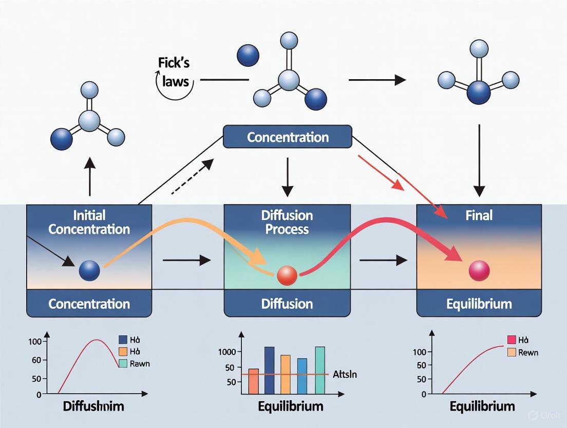
Diffusion describes the random movement of particles from a region of high concentration to a region of low concentration, driven by a concentration gradient to ultimately achieve uniform distribution [1] [2]. This spontaneous process results from random thermal motions and serves as a fundamental mass transfer mechanism across scientific and engineering disciplines [3]. First mathematically described by Adolf Fick in 1855, diffusion principles form the core of our understanding of transport in gases, liquids, and solids [4] [1]. In biological systems, diffusion governs crucial processes including gas exchange in lungs, drug delivery mechanisms, and cellular signaling [5] [1], while industrial applications span pharmaceutical development, semiconductor fabrication, food processing, and environmental remediation [1] [6]. This technical guide provides an in-depth examination of diffusion theory, experimental methodologies, and research applications framed within contemporary molecular diffusion research.

Theoretical Foundations

Fundamental Principles

Diffusion occurs as a statistical consequence of random particle movements in a concentration gradient. Each particle moves independently, with the net directional flow occurring from high to low concentration regions due to purely probabilistic considerations [3] [2]. The diffusion coefficient (D) quantifies how quickly particles spread through a medium, with dimensions of area per time (m²/s) [4] [3]. This coefficient depends on temperature, viscosity, and particle size according to the Stokes-Einstein relation [4] [3]:

Table 1: Typical Diffusion Coefficient Values

System Type	Diffusion Coefficient Range (m²/s)	Examples
Ions in solution	0.6×10⁻⁹ to 2×10⁻⁹	Na⁺, Cl⁻ in water
Biological molecules	10⁻¹¹ to 10⁻¹⁰	Proteins, DNA
Gases	10⁻⁶ to 10⁻⁵	Oxygen in air

Two operational regimes characterize diffusion processes: steady-state diffusion occurs when concentration profiles remain constant over time (∂c/∂t = 0), while transient diffusion involves time-dependent concentration changes [2].

Fick's First Law

Fick's first law describes steady-state diffusion where the concentration profile does not change with time [4] [2]. It establishes that the diffusive flux is proportional to the negative concentration gradient:

For one-dimensional systems: J = -D(dφ/dx)

For multi-dimensional systems: J = -D∇φ

where J represents the diffusion flux (amount of substance per unit area per unit time), D is the diffusion coefficient, φ denotes concentration, and x is position [4]. The negative sign indicates that diffusion occurs down the concentration gradient [1]. In biological systems, Fick's first law generates the permeability equation: Diffusion Flux = -P(c₂-c₁), where P represents an experimentally determined membrane conductance [1].

Fick's Second Law

Fick's second law predicts how diffusion causes concentrations to change with time, making it essential for modeling transient diffusion processes [4] [3]. This partial differential equation relates temporal concentration changes to spatial variations:

For one-dimensional systems: ∂φ/∂t = D(∂²φ/∂x²)

For multi-dimensional systems: ∂φ/∂t = D∇²φ

where ∂φ/∂t represents the rate of concentration change over time [4] [7]. The second law derives from applying mass conservation to Fick's first law, assuming constant diffusion coefficient [4]. This equation shares identical mathematical form with the heat equation, enabling cross-disciplinary application of solution methods [4].

Experimental Methodologies

Laboratory-Scale Diffusion Analysis

Investigating diffusion phenomena at laboratory scale requires carefully controlled conditions to isolate mechanistic behavior. The following protocol, adapted from groundwater contaminant transport research, provides a robust methodology for visualizing and quantifying diffusion processes [6].

Experimental Setup for Diffusion Visualization

• Apparatus: Plexiglas tank (68cm × 40cm × 7cm) divided into mixing and porous media chambers
• Porous Media: High-permeability quartz sand (Dâ‚…â‚€ = 700μm) with embedded low-permeability lenses
• Tracer Selection: Sodium fluorescein (2g/L concentration) selected for non-toxidity, visibility, and fluorescence properties
• Monitoring System: 3CCD camera with UV illumination (Philips Actinic BL TL-D 18W-10 UV-A G13) for excitation
• Flow Control: Peristaltic pumps maintaining constant flow rate (~26 mL/min)

Experimental Procedure

• System Saturation: Completely saturate tank with deionized water to eliminate air pockets
• Tracer Introduction: Slowly inject fluorescein solution into mixing chamber
• Effluent Monitoring: Collect outlet samples periodically for fluorometer analysis
• Image Acquisition: Capture RGB format images during flushing and rest phases
• Data Processing: Apply Image Analysis techniques to determine concentration fields
• Flux Calculation: Compute diffusive fluxes from low-permeability zones using concentration gradients

This experimental design enables direct observation of both forward diffusion (into low-permeability zones) and back-diffusion (release from these zones), critical processes in environmental remediation and drug delivery systems [6].

Research Reagent Solutions

Table 2: Essential Research Materials for Diffusion Experiments

Reagent/Material	Specification	Function in Experimental System
Sodium Fluorescein	2g/L in aqueous solution	Colored tracer for visualization and quantification
Quartz Sand	D₅₀ = 700μm, porosity ~0.3	High-permeability matrix simulating aquifer or biological environment
Quartz Flour	D₅₀ = 12-15μm, porosity ~0.4	Low-permeability lens material for diffusion studies
Sodium Bentonite	D₅₀ = 1.3μm, porosity ~0.5	Very low-permeability material for contrast studies
UV Light Source	254nm wavelength	Fluorescein excitation for image analysis

Boundary Conditions in Diffusion Analysis

Appropriate boundary conditions are essential for solving Fick's laws across experimental and modeling applications [7]:

Dirichlet Conditions: Specify concentration values at system boundaries

• Constant surface concentration (e.g., saturated solution interface)
• Fixed concentration ratio at membrane boundaries

Neumann Conditions: Define flux values at system boundaries

• Constant flux application (e.g., evaporation rate)
• Impermeable boundary (zero flux condition)

Robin Conditions: Combine concentration and flux relationships

• Convective mass transfer at interfaces
• Reaction-diffusion boundaries in biological systems

Table 3: Boundary Condition Applications in Diffusion Models

Condition Type	Mathematical Form	Common Applications
Dirichlet	c(0,t) = câ‚€	Constant source concentration, saturated systems
Neumann	-D(∂c/∂x) = J₀	Controlled release systems, evaporation
Robin	-D(∂c/∂x) = h(c - c∞)	Convective mass transfer, reaction interfaces

Advanced Applications and Research Implications

Pharmaceutical and Drug Development

In drug development, diffusion principles govern critical processes from API synthesis to targeted delivery systems. Membrane diffusion according to Fick's first law determines drug release rates from controlled-release formulations, with permeability coefficients optimized for specific therapeutic windows [1]. Back-diffusion phenomena from tissue reservoirs create long-term release profiles that impact dosing regimens and therapeutic efficacy [6]. Understanding these mechanisms enables rational design of nanocarrier systems and diffusion-controlled delivery platforms.

Environmental Remediation

Contaminant transport in groundwater systems exemplifies complex diffusion applications. Low-permeability zones act as contaminant reservoirs through forward diffusion during plume passage, followed by long-term back-diffusion that sustained concentration tails after primary source removal [6]. This process undermines remediation efforts and necessitates sophisticated models incorporating Fick's laws with hydrological parameters. Research demonstrates that diffusion-dominated transport in heterogeneous aquifers requires characterization of both high-permeability pathways and low-permeability storage zones for accurate prediction of contaminant persistence.

Biological and Medical Systems

Molecular diffusion within cellular environments presents unique challenges due to crowding, binding interactions, and compartmentalization. Intracellular diffusion coefficients for biological molecules typically range from 10⁻¹¹ to 10⁻¹⁰ m²/s, significantly lower than in dilute solutions due to molecular crowding [4] [3]. Educational visualization of these processes must balance accuracy with conceptual clarity, addressing common misconceptions about molecular agency while representing random thermal motion realistically [5]. Advanced imaging techniques combined with computational modeling based on Fick's laws enable quantification of transmembrane transport rates critical for understanding drug uptake and nutrient exchange.

Diffusion, mathematically formalized through Fick's laws, remains a cornerstone transport phenomenon with expanding applications across scientific and engineering disciplines. The fundamental principles established 170 years ago continue to inform contemporary research in pharmaceutical development, environmental management, and biological systems. Current challenges include extending diffusion theory to non-Fickian regimes, multi-component systems, and heterogeneous environments where classical relationships require modification. Emerging visualization and computational technologies enable increasingly sophisticated investigation of diffusion processes across spatial and temporal scales, ensuring continued relevance of these fundamental transport principles in addressing complex research and application challenges.

In 1855, a 26-year-old German physician and physiologist, Adolf Eugen Fick(1829-1901), published his seminal paper "Ãœber Diffusion" in Annalen der Physik, establishing the fundamental laws of diffusion that bear his name [8] [9]. Fick, who excelled in mathematics and physics, approached physiology with a rigorous, quantitative mindset, believing that physical laws governing mass and energy transport were essential to understanding biological systems [8]. His work was inspired by earlier experiments on gases by Thomas Graham and drew a direct mathematical analogy to Jean-Baptiste Joseph Fourier's law of heat conduction [4] [9]. Remarkably, Fick first formulated his laws based on this theoretical analogy and physical reasoning, with experimental verification following the theoretical work [8] [10]. This groundbreaking publication not only laid the foundation for modern diffusion theory but also exemplified cross-disciplinary research, impacting fields from physical chemistry and engineering to medicine and materials science [9].

Theoretical Foundations: Fick's Laws of Diffusion

The Core Principles

Fick's laws provide a complete mathematical description of diffusion, defining the relationship between concentration gradients, flux, and temporal changes.

Table 1: Core Principles of Fick's Laws of Diffusion

Law	Mathematical Expression	Key Variables	Fundamental Principle
Fick's First Law	J = -D(dφ/dx)	J: Diffusion Flux [(mol/m²s)]D: Diffusion Coefficient [(m²/s)]φ: Concentration [(mol/m³)]x: Position [m]	The diffusive flux is proportional to the negative concentration gradient. It describes movement from high to low concentration.
Fick's Second Law	∂φ/∂t = D(∂²φ/∂x²)	t: Time [s]φ: Concentration [(mol/m³)]D: Diffusion Coefficient [(m²/s)]x: Position [m]	The rate of change of concentration over time is proportional to the second derivative of the concentration gradient.

Mathematical and Conceptual Analogy

Fick conceptualized diffusion as a binary process where solute particles move in one direction while water moves in the other [10]. He intuitively understood that the concentration gradient served as the driving force for this spontaneous process, analogous to how a temperature gradient drives heat flow [4] [9]. His first law provides a steady-state description, while the second law predicts how concentration evolves in non-steady-state, time-dependent scenarios [4] [3]. A process that obeys these relationships is termed normal or Fickian diffusion, while those that do not are classified as anomalous or non-Fickian diffusion [4] [11].

The 1855 Experiments: Methodology and Validation

Experimental Design and Setup

Fick's experimental validation, detailed in "On Liquid Diffusion," was elegantly simple yet powerful. His apparatus consisted of two reservoirs containing salt solutions at different concentrations, connected by a tube filled with water [4] [12]. This design allowed him to measure the concentrations and fluxes of salt diffusing between the reservoirs under a controlled concentration gradient [4]. He sought to test the hypothesis that the movement of particles in a solution could be described by the same mathematical formalism Fourier had established for heat flow [10] [9].

Table 2: Key Research Reagents and Materials in Fick's Experiments

Research Reagent/Material	Function in the Experiment
Salt (Solute)	The diffusing species whose transport was measured. Its concentration gradient provided the driving force for diffusion.
Water (Solvent)	The fluid medium within the connecting tube through which the salt diffusion occurred.
Glass Tube	Provided a confined, linear path for one-dimensional diffusion, simplifying the measurement of flux and gradient.
Fluid Membranes/Barriers	Used to study implications of binary diffusion and transport in more complex systems, relevant to biological membranes [10].

Protocol and Workflow

The following diagram outlines the general workflow derived from Fick's pioneering experimental approach.

Quantitative Findings and Diffusion Coefficients

Fick's experiments allowed him to verify the proportional relationship between flux and concentration gradient. While his original work focused on establishing this relationship, subsequent research has quantified diffusion coefficients for various substances, which are critical for practical applications.

Table 3: Typical Diffusion Coefficient (D) Values in Aqueous Solutions at Room Temperature

Substance Category	Diffusion Coefficient (m²/s)	Notes
Ions	0.6 × 10⁻⁹ to 2 × 10⁻⁹	Relatively similar values in dilute aqueous solutions [4].
Biological Molecules	10⁻¹¹ to 10⁻¹⁰	Larger molecules result in slower diffusion [4] [3].
Small Gases/Molecules	~10⁻⁹	Order of magnitude estimate for small solutes in water.

The diffusion coefficient itself depends on factors such as temperature, viscosity of the fluid, and the size of the diffusing particles, as later described by the Stokes-Einstein relation [4] [3].

Beyond the Basics: Nuances and Later Refinements

Fick's Original Conceptualization

A careful reading of Fick's 1855 paper reveals that his conceptualization was more comprehensive than the common simplification of his first law. He visualized diffusion as a binary process with simultaneous counter-movement of salt and water [10]. He also intuitively described what would later be formalized as chemical potential, referring to a "force of suction... proportional to the difference of concentration" [10]. Furthermore, he dedicated significant discussion to the implications of diffusion through membranes, making his work immediately relevant to biological systems [10].

Modern Critiques and the Limits of Fick's Laws

While Fick's laws are foundational, their limitations in certain physical regimes have been a subject of ongoing research. For over a century, it has been recognized that concentration gradient is not the true thermodynamic driving force; rather, it is the gradient of chemical potential [13]. However, research in the 21st century has suggested that even the chemical potential gradient may not be the complete picture in all cases, and that the fundamental equation might require modification, especially in systems with large mean free paths (e.g., low-pressure gases, nanoporous materials) where wave-like density phenomena can occur [13]. These are active areas of research, demonstrating that the understanding of diffusion, initiated by Fick, continues to evolve.

Applications and Impact Across Disciplines

Fick's laws of diffusion have transcended their origin in physiology to become a cornerstone of modern science and technology.

• Biological and Medical Sciences: Fick's laws are fundamental to understanding gas exchange in the lungs (a application Fick himself pioneered with the Fick principle for cardiac output) [8], nutrient and drug transport across cell membranes [11] [14], and the design of controlled-release pharmaceuticals [11] [14].
• Semiconductor Fabrication: The diffusion equations are critical for processes like doping, where impurity atoms are diffused into silicon wafers to modulate electronic properties [11] [14].
• Materials Science and Engineering: Applications include modeling the carburization of steel, hydrogen storage in metals, and the development of novel materials [14].
• Food Science: Diffusion principles are applied to processes such as salting, drying, and flavoring [11].
• Environmental Engineering: Used to model the spread of contaminants in groundwater and pollutants in the atmosphere [12] [9].

Adolf Fick's 1855 work represents a paradigm shift in how scientists conceptualize and quantify the spontaneous mixing of substances. By forging a powerful analogy between mass and heat transport, he provided a mathematical framework that has proven remarkably durable and widely applicable. His laws remain the essential starting point for modeling transport phenomena across an immense spectrum of scientific and engineering disciplines. While modern research continues to explore the boundaries and refine the theory, particularly for non-Fickian and anomalous diffusion, Fick's groundbreaking insight continues to underpin our fundamental understanding of diffusion.

Fick's laws of diffusion, first posited by physiologist Adolf Fick in 1855, form the foundational framework for understanding molecular diffusion [4]. Inspired by the earlier experiments of Thomas Graham and analogous to contemporary scientific relationships like Ohm's law for charge transport and Fourier's law for heat transport, Fick's work established the fundamental principles governing the transport of mass through diffusive means [4]. Within this framework, Fick's First Law provides the essential relationship between the diffusive flux and the underlying concentration gradient that drives the process. This article presents an in-depth technical examination of Fick's First Law, detailing its physical meaning, mathematical expression, and derivation, with specific consideration for its applications in scientific research and drug development.

Physical Meaning of the Diffusion Flux

Conceptual Foundation

Diffusion can be described as the random movement of particles through space, typically due to a concentration gradient, and represents a spontaneous process resulting from random thermal motions between particles [3]. At its core, Fick's First Law postulates that the diffusive flux moves from regions of high concentration to regions of low concentration, with a magnitude proportional to the concentration gradient (spatial derivative) [4]. In more simplistic terms, the law encapsulates the concept that a solute will move from a region of high concentration to a region of low concentration across a concentration gradient [4].

The driving force for one-dimensional diffusion is the quantity −∂φ/∂x, which for ideal mixtures is the concentration gradient [4]. This spontaneous flow occurs as particles undergo random thermal motions, leading to a net displacement from regions of higher chemical potential to regions of lower chemical potential [3].

Definition of Diffusion Flux

In the context of Fick's First Law, the diffusion flux, typically denoted by J, is defined as the amount of substance that flows through a unit area during a unit time interval [4]. Mathematically, flux is defined by the number of particles moving past a given region divided by the area of that region multiplied by the time interval [3]. The standard units for flux are mol m⁻² s⁻¹, though variations exist depending on the specific formulation of the law and the system of units employed [3].

Table 1: Key Parameters in Fick's First Law

Parameter	Symbol	Definition	Typical Units
Diffusion Flux	J	Amount of substance flowing through unit area per unit time	mol m⁻² s⁻¹
Concentration	φ, c	Amount of substance per unit volume	mol m⁻³
Position	x	Distance along diffusion direction	m
Diffusion Coefficient	D	Proportionality constant characterizing mobility of diffusing species	m² s⁻¹
Concentration Gradient	dφ/dx, dc/dx	Spatial rate of change of concentration	mol m⁻⁴

Mathematical Expression of Fick's First Law

Fundamental Equation

The fundamental mathematical expression of Fick's First Law in one spatial dimension states that the diffusion flux is proportional to the negative concentration gradient [4] [3]. The most common form of the equation, expressed in a molar basis, is:

[ J = -D \frac{d\varphi}{dx} ]

where:

• J is the diffusion flux [mol m⁻² s⁻¹]
• D is the diffusion coefficient or diffusivity [m² s⁻¹]
• dφ/dx is the concentration gradient [mol m⁻⁴]
• φ is the concentration [mol m⁻³]
• x is the position [m] [4] [3]

The negative sign in the equation indicates that the direction of diffusion is opposite to the direction of increasing concentration – meaning flow occurs from high to low concentration regions [4] [3].

Variations and Alternative Formulations

Several variations of Fick's First Law exist for different applications and systems. When expressed with the primary variable as mass fraction (y_i), the equation becomes:

[ \mathbf{J}i = -\frac{\rho D}{Mi} \nabla y_i ]

where:

• the index i denotes the ith species
• J_i is the diffusion flux of the ith species [mol m⁻² s⁻¹]
• M_i is the molar mass of the ith species
• ρ is the mixture density [kg m⁻³]
• y_i is the mass fraction of the ith species [4]

For chemical systems other than ideal solutions or mixtures, where the driving force is the gradient of chemical potential, Fick's First Law can be written as:

[ Ji = -\frac{D ci}{RT} \frac{\partial \mu_i}{\partial x} ]

where:

• c_i is the concentration [mol m⁻³]
• R is the universal gas constant [J K⁻¹ mol⁻¹]
• T is the absolute temperature [K]
• μ_i is the chemical potential [J mol⁻¹] [4]

In two or more dimensions, the gradient operator (∇) generalizes the first derivative, resulting in:

[ \mathbf{J} = -D \nabla \varphi ]

where J and ∇φ are vector quantities [4].

Table 2: Diffusion Coefficient Values for Different Systems

System Type	Diffusing Species	Typical D Values [m²/s]	Conditions
Aqueous Solutions	Ions	0.6–2 × 10⁻⁹	Room Temperature [4]
Biological Systems	Molecules	10⁻¹¹ – 10⁻¹⁰	Room Temperature [4]
Gases	COâ‚‚ in n-alkanes	Variable with pressure	High-pressure reservoirs [15]

Derivation of Fick's First Law

Atomic-Scale Derivation Using the Random Walk Model

The derivation of Fick's First Law can be approached by considering atomic-scale motion within a crystal lattice, modeling diffusion as a random walk process [16]. Consider a crystal structure where each plane contains Cλ atoms per unit area, where C is the concentration and λ is the jump distance between atomic planes [16].

For an increment of distance (δx) of λ, the corresponding increment of concentration (δC) is given by:

[\partial C = \lambda \left{ {\frac{{\partial C}}{{\partial x}}} \right}] [16]

In a three-dimensional crystal, an atom can move in one of six directions. If the jump frequency is ν, the fluxes of atoms from left to right and from right to left are given by:

[{J{L \to R}} = \frac{1}{6}\nu C\lambda ] [{J{R \to L}} = \frac{1}{6}\nu (C + \partial C)\lambda ] [16]

The net flux J is therefore:

[ J = {J{L \to R}} - {J{R \to L}} ] [ J = - \frac{1}{6}\nu \partial C\lambda ] [ J = - \frac{1}{6}\nu \left{ {\frac{{\partial C}}{{\partial x}}} \right}{\lambda ^2} ] [ J \equiv - D\left{ {\frac{{\partial C}}{{\partial x}}} \right} ] [16]

where D = (1/6)νλ² is identified as the diffusivity of the diffusing species [16]. This derivation establishes Fick's First Law from fundamental atomic-scale motions.

Continuum Derivation from Mass Conservation

An alternative derivation approaches diffusion from a continuum perspective, considering the flow of particles due to a concentration gradient across a membrane [17] [18]. This approach defines the flow of particles across a membrane as:

[ J_{\text{diffusion}} = -D \frac{d[I]}{dx} ]

where J is the flow of particles due to diffusion, [I] is the ion concentration, dx is the membrane thickness, and D is the diffusivity constant [m²/s] [17]. The negative sign indicates that the flow of ions is from higher to lower concentration [17].

This derivation can be visualized by considering a still liquid in a long pipe of constant cross-sectional area, where a small quantity of dye is placed in a cross-section and allowed to diffuse [18]. Defining u(x,t) as the concentration of dye at position x along the pipe, Fick's law of diffusion assumes the mass flux J across a cross-section is given by:

[ J = -D u_x ]

where u_x = ∂u/∂x, and D > 0 is the diffusion constant [18].

Experimental Protocols and Research Methodologies

Molecular Dynamics Approaches

Modern computational methods enable the calculation of Fick diffusion coefficients through molecular dynamics simulations [15]. The modified Fourier Correlation Method (mFCM) represents an innovative approach to calculate binary Fick diffusion coefficients directly through equilibrium molecular dynamics (EMD) simulations [15].

Protocol: Modified Fourier Correlation Method (mFCM)

• System Setup: Create a molecular model of the binary mixture of interest (e.g., COâ‚‚ and n-alkane mixtures) at specified temperature, pressure, and composition conditions [15].

• Equilibrium Simulation: Perform equilibrium molecular dynamics (EMD) simulations to generate trajectory data of molecular positions and velocities over time [15].

• Structure Factor Calculation: Compute the partial time-dependent structure factors S_ij(q,t) from the EMD trajectories [15].

• Diffusion Coefficient Extraction: Determine the binary Fick diffusion coefficient D₁₂ by analyzing the decay of concentration fluctuations in the Fourier domain, using the relationship:

  [ \frac{dS{ij}(q,t)}{dt} = -D{12}(q)q^2S_{ij}(q,t) ]

  which has the solution:

  [ S{ij}(q,t) = S{ij}(q,0)e^{-D_{12}(q)q^2t} ]

  where D₁₂(q) is the wavenumber-dependent Fick diffusion coefficient [15].

• Thermodynamic Limit Evaluation: Assess finite-size effects and extrapolate to the thermodynamic limit, as the mFCM approach considerably reduces the finite-size effect of the simulation box on calculated diffusion coefficients [15].

Traditional Experimental Approaches

While molecular dynamics offers powerful computational approaches, traditional experimental methods remain valuable for measuring diffusion coefficients:

Protocol: Traditional Diffusion Cell Method

• Apparatus Setup: Utilize a diffusion cell consisting of two well-mixed reservoirs separated by a permeable membrane or capillary tube [4].

• Initial Conditions: Establish different initial concentrations in each reservoir to create a known concentration gradient across the membrane [4].

• Flux Measurement: Monitor the change in concentration in one or both reservoirs over time to determine the flux J [4].

• Diffusion Coefficient Calculation: Apply Fick's First Law (J = -D·dc/dx) to calculate the diffusion coefficient D from the measured flux and the known concentration gradient [4].

Table 3: Research Reagent Solutions for Diffusion Studies

Reagent/Material	Function in Experiment	Application Context
Binary Fluid Mixtures (e.g., COâ‚‚ + n-alkane)	Model system for studying mutual diffusion	High-pressure mass transfer, reservoir engineering [15]
Isotopically Labeled Compounds	Tracers for tracking diffusion pathways	Self-diffusion measurements in multicomponent systems [15]
Polymer Membranes	Barrier for studying vapour transmission	Packaging materials, drug delivery systems [19]
Electrolyte Solutions	Study ion diffusion in aqueous systems	Biological systems, battery research [4] [3]
Porous Media	Matrix for studying confined diffusion	Geology, construction materials, drug delivery [17]

Applications in Drug Development and Research

Fick's First Law finds critical applications in pharmaceutical research and drug development, particularly in the design and optimization of drug delivery systems [20]. Understanding and controlling diffusion processes enables the development of controlled drug delivery systems that combat problems associated with conventional drug delivery, such as poor bioavailability and fluctuations in plasma drug levels [20].

In transdermal drug delivery, Fick's First Law directly informs the design of patches where the rate of drug transfer through the skin is proportional to the concentration difference across the skin layers and inversely proportional to the thickness of the membrane [19]. Similarly, in oral dosage forms, the dissolution and subsequent diffusion of active pharmaceutical ingredients (APIs) through gastrointestinal membranes follow the principles established by Fick's First Law [20].

The Biopharmaceutics Classification System (BCS) classifies drugs into four categories based on their solubility and permeability characteristics, with Fick's First Law providing the fundamental basis for understanding the permeability aspects [20]. For BCS Class II drugs (high permeability, low solubility) and BCS Class IV drugs (low permeability, low solubility), diffusion limitations significantly impact bioavailability, necessitating sophisticated formulation strategies grounded in Fick's principles [20].

Limitations and Considerations

While Fick's First Law provides a fundamental description of diffusion processes, several limitations and considerations must be acknowledged for accurate application in research contexts:

• Finite Medium Effects: Fick's law is derived for an infinite homogeneous medium, while real systems often have boundaries. The law remains valid for points away from edges by few mean free paths [17].

• Nonuniform Media: For nonuniform media where scattering properties change sharply, Fick's law requires modification or re-evaluation, though it remains valid provided sharp changes don't lead to rapid flux variation [17].

• Proximity to Sources or Sinks: Near strong sources or sinks, Fick's law may break down, though it remains valid at few mean free paths away from such boundaries [17].

• Anisotropic Scattering: The assumption of isotropic scattering is not generally true. With moderate anisotropy, Fick's law can be used with a modified diffusion coefficient [17].

• Highly Absorbing Media: In highly absorbing media where the flux varies rapidly spatially, higher-order terms may be necessary, and exact transport theory may be more appropriate [17].

• Time-Dependent Flux: For time-dependent fluxes, Fick's law assumes instantaneous propagation, while physically there is finite travel time between collisions [17].

Fick's First Law provides the fundamental relationship between diffusive flux and concentration gradients, serving as a cornerstone for understanding mass transport phenomena across numerous scientific disciplines. From its basis in atomic-scale random walk processes to its manifestations in continuum systems, the law establishes a proportional relationship between flux and concentration gradient with the diffusion coefficient as the constant of proportionality. While the law has limitations in specific scenarios, modern research methodologies including molecular dynamics simulations continue to extend its applicability and precision. For drug development professionals and researchers, Fick's First Law remains an essential principle for designing and optimizing delivery systems, understanding bioavailability limitations, and developing controlled release strategies that maximize therapeutic efficacy while minimizing adverse effects.

Fick's second law is a fundamental partial differential equation that describes how the concentration of a substance changes with time due to diffusion. This law serves as the cornerstone for predicting time-dependent diffusion processes across numerous scientific and engineering disciplines, from pharmaceutical drug release to materials science. While Fick's first law describes the steady-state flux of particles under a constant concentration gradient, the second law addresses the more common non-steady-state scenarios where concentrations evolve over time [4] [17].

Derived from Fick's first law combined with the principle of mass conservation, Fick's second law mathematically expresses how the rate of change of concentration at a point in space is proportional to the second derivative of the concentration field [4] [21]. For one-dimensional systems, this is expressed as ∂C/∂t = D(∂²C/∂x²), where C represents concentration, t is time, x is position, and D is the diffusion coefficient [22] [4] [23]. In multiple dimensions, this generalizes to ∂C/∂t = D∇²C, where ∇² is the Laplace operator [4].

The following diagram illustrates the fundamental relationship between Fick's first and second laws and their role in describing diffusion phenomena:

Fundamental Theory and Mathematical Formulation

Core Equation and Physical Interpretation

Fick's second law establishes that the time evolution of concentration is governed by the spatial curvature of the concentration profile. Where the concentration profile is concave up (positive second derivative), the concentration at that point will increase with time; where it is concave down (negative second derivative), the concentration will decrease [4]. The diffusion coefficient D (m²/s) determines the rate at which this process occurs and is typically temperature-dependent, following an Arrhenius relationship: D = D₀exp(-Eₐ/kBT) [23].

The derivation of Fick's second law combines Fick's first law, which states that the diffusive flux J is proportional to the negative concentration gradient (J = -D∂C/∂x), with the continuity equation from mass conservation (∂C/∂t = -∂J/∂x) [4] [21]. Substituting the first law into the continuity equation yields Fick's second law, assuming a constant diffusion coefficient [4] [21]. This derivation highlights how the second law naturally emerges from the conservation of mass when combined with the linear response approximation of the first law.

Analytical Solutions for Key Boundary Conditions

For specific initial and boundary conditions, Fick's second law admits exact analytical solutions that provide profound insight into diffusion behavior. The two most fundamental cases are the "thin source" and "infinite source" scenarios [22] [24].

Table 1: Boundary Conditions and Solutions for Fick's Second Law

Scenario	Boundary Conditions	Solution	Application Examples
Thin Source	Fixed amount of solute B in semi-infinite medium; Initial concentration = 0 [22] [24]	C(x,t) = B/√(πDt) · exp(-x²/(4Dt)) [22] [24]	Dopant diffusion in semiconductors; tracer studies
Infinite Source	Constant surface concentration Cₛ in semi-infinite medium; Initial concentration = C₀ [22] [23] [24]	C(x,t) = Cₛ - (Cₛ - C₀) · erf(x/(2√Dt)) [22] [23] [24]	Case hardening of metals; drug release from transdermal patches

The error function (erf) in the infinite source solution arises from integrating Gaussian distributions and is defined as erf(z) = (2/√π) ∫₀^z exp(-u²) du [22] [24]. This function exhibits a characteristic s-shaped profile that gradually penetrates deeper into the material over time, with the diffusion front progressing proportionally to √Dt [22] [23].

The following workflow illustrates how these analytical solutions are derived and applied to solve practical diffusion problems:

Experimental Methodologies and Measurement Techniques

Research Reagent Solutions and Materials

Table 2: Essential Research Reagents and Materials for Diffusion Studies

Reagent/Material	Function/Application	Example Specifications
Liposome Vesicles	Model membrane system for drug diffusion studies [25]	POPC phospholipids; 30-100 nm diameter [25]
Polyethylene Glycol (PEG)	Polymer steric stabilizer for "stealth" liposomes [25]	Molecular weight: 1-10 kDa; conjugated to lipid heads [25]
Sucrose Solutions	Diffusion rate modifier in layered experimental systems [25]	Concentration: 0.1-1.0 M; D ≈ 4.586×10⁻¹⁰ m²/s [25]
Solid Lipid Nanoparticles (SLNs)	Alternative drug carrier system with Fickian release [25]	Composed of solid lipids stabilized with emulsifying layer [25]
Optical-Clearing Reagents	Enhance tissue transparency for diffusion imaging [25]	Commercially available formulations (e.g., FocusClear) [25]

Protocol for Thin Source Diffusion Measurement

Objective: Quantify the diffusion coefficient of a tracer substance in a solid or gel matrix using the thin source method [22] [24].

Materials Preparation:

• Prepare sample plates of the matrix material with polished, parallel surfaces
• Create a thin layer of tracer material through vapor deposition, spin-coating, or brief immersion in a concentrated solution
• For radioactive tracers, ensure proper safety protocols and detection equipment

Experimental Procedure:

• Assemble the diffusion couple with the tracer layer at the interface
• Place in a temperature-controlled furnace or environmental chamber at the target temperature (±0.5°C)
• Maintain for predetermined time intervals (typically hours to days depending on D)
• Rapidly quench samples to room temperature to stop diffusion
• Section samples perpendicular to the diffusion direction and prepare for concentration profiling

Concentration Profiling:

• For chemical tracers: Use techniques like SEM-EDS, SIMS, or spectroscopic methods
• For radioactive tracers: Employ autoradiography or sequential sectioning with counting
• Measure concentration as a function of distance from the initial interface

Data Analysis:

• Plot concentration versus distance profiles for each diffusion time
• Fit data to the thin source solution: C(x,t) = B/√(πDt) · exp(-x²/(4Dt))
• Extract D from the Gaussian width parameter using the relationship: σ² = 2Dt
• Repeat at multiple temperatures to determine activation energy Eₐ

Advanced Applications and Current Research Frontiers

Drug Delivery Systems

Fick's second law provides the theoretical foundation for controlled-release drug delivery systems. In transdermal patches, the law predicts how drug molecules diffuse through skin layers over time, enabling optimization of therapeutic dosing [25]. Multi-vesicular liposomes employ concentric phospholipid bilayers to create diffusion barriers that control drug release kinetics according to Fickian principles [25]. Recent advances include "stealth liposomes" that use surface-grafted polyethylene glycol to evade immune detection while maintaining controlled diffusion profiles [25].

Numerical solutions of Fick's second law enable the design of complex multi-layered drug delivery systems. Researchers have demonstrated that specific layer sequences can create near-constant release rates (zero-order kinetics) by maintaining a constant concentration gradient at the delivery interface [25]. Finite-element simulations of Fick's law accurately predict how different layer compositions and thicknesses affect the temporal release profile, reducing experimental optimization time.

Diffusion Cloaking and Transformation Thermodynamics

A cutting-edge application of Fick's second law emerges in the field of diffusion cloaking, where engineered materials are designed to control mass flux in unconventional ways [25]. By creating composite structures with specifically ordered layers of different diffusivities, researchers can guide diffusion fronts around enclosed regions, effectively "hiding" objects from diffusing species [25]. This approach, derived from transformation thermodynamics, uses coordinate transformations of Fick's equation to design material parameters that manipulate diffusion pathways [25].

Experimental realizations have employed concentric layered structures with alternating high and low diffusivity materials. For example, a liposome nanoparticle (D ≈ 1.9×10⁻¹¹ m²/s) surrounded by alternating sucrose (D ≈ 4.586×10⁻¹⁰ m²/s) and chloroform (higher D) layers can exhibit markedly different external concentration profiles compared to uncloaked particles [25]. These structured diffusion media can maintain higher internal concentrations for extended periods, potentially enhancing drug stability and circulation time [25].

Numerical Approaches for Complex Systems

For realistic geometries, variable diffusion coefficients, or coupled physical processes, numerical methods are essential for solving Fick's second law [22] [24] [21]. The finite difference method discretizes the partial differential equation onto a spatial grid and marches forward in time using explicit or implicit schemes [22]. The finite element method handles complex geometries and boundary conditions more effectively, making it suitable for biological tissues or engineered devices with irregular shapes [25].

Commercial packages like COMSOL Multiphysics implement Fick's second law alongside other physics for coupled simulation of heat transfer, fluid flow, and chemical reaction [21]. For multi-component systems where diffusion coefficients depend on composition, the Maxwell-Stefan equations extend Fick's approach to account for inter-species interactions [21]. These advanced implementations remain rooted in the fundamental principles established by Fick's second law while addressing its limitations for concentrated solutions.

Table 3: Numerical Methods for Solving Fick's Second Law

Method	Key Features	Implementation Considerations
Finite Difference	Simple implementation; Direct discretization of derivatives [22]	Stability limits (∆t ∝ (∆x)²); Suitable for regular geometries
Finite Element	Handles complex geometries; Adaptive meshing [25]	Higher computational cost; More complex implementation
Finite Volume	Conservative by construction; Handles discontinuous coefficients	Intermediate complexity; Widely used in fluid dynamics
Boundary Element	Reduces dimensionality; Only requires surface discretization	Dense matrices; Challenging for nonlinear problems

Limitations and Extensions of Fick's Second Law

While Fick's second law provides an excellent description of diffusion in many systems, several important limitations must be recognized. The law assumes a constant diffusion coefficient, which fails for concentrated solutions where D becomes concentration-dependent [4] [21]. In such cases, the more general form ∂C/∂t = ∇·(D(C)∇C) must be used [4]. The derivation also assumes isotropic scattering and homogeneous media, limitations particularly relevant in neutron diffusion and composite materials [17].

Anomalous diffusion refers to cases where the mean squared displacement follows ⟨x²⟩ ∝ t^α with α ≠ 1, violating the fundamental assumption of Fickian diffusion [4]. This occurs in porous media, polymer networks, and intracellular environments where obstacles and binding sites create complex energy landscapes for diffusing particles [4] [17]. For such systems, fractional derivative formulations may better describe the transport physics.

When advection accompanies diffusion, the convection-diffusion equation extends Fick's second law: ∂C/∂t + v·∇C = D∇²C, where v is the velocity field [25] [21]. This coupled equation describes many environmental and physiological transport processes where bulk fluid motion significantly contributes to mass transfer. Similarly, reaction-diffusion systems incorporate source terms: ∂C/∂t = D∇²C + R(C), enabling modeling of chemical patterning and biological morphogenesis [25].

Within the study of molecular diffusion, the diffusion coefficient, denoted as (D), serves as a fundamental kinetic parameter that quantifies the rate at which particles spread from regions of high concentration to low concentration. This transport phenomenon, critical across disciplines from chemical engineering to pharmaceutical sciences, is macroscopically described by Fick's laws of diffusion [3]. The value of the diffusion coefficient is not an intrinsic constant; it is highly sensitive to environmental conditions, with temperature exerting one of the most profound influences. This temperature dependence is powerfully captured by the Arrhenius equation, a cornerstone of physical chemistry that relates the rate of a process to the thermal energy available to the system [26] [27].

Framed within a broader thesis on the theory of molecular diffusion, this whitepaper provides an in-depth examination of the diffusion coefficient. It will elucidate its physical significance, establish its fundamental units, and explore its temperature-driven behavior through the lens of the Arrhenius relationship. The discussion is extended to include practical methodologies for its experimental determination, providing researchers and drug development professionals with a comprehensive technical guide.

Theoretical Foundations of Diffusion

Fick's Laws of Diffusion

The mathematical framework for diffusion was established by Adolf Fick in the 19th century. His two laws form the bedrock of quantitative diffusion analysis.

• Fick's First Law describes the steady-state flux, where the concentration profile does not change with time. It states that the diffusive flux, (J), is proportional to the negative of the concentration gradient [3]. The law is expressed as: [ J = -D \dfrac{dc}{dx} ] where:

  • (J) is the flux density (mol m⁻² s⁻¹),
  • (D) is the diffusion coefficient (m²/s),
  • (\dfrac{dc}{dx}) is the spatial concentration gradient (mol m⁻⁴). The negative sign indicates that diffusion occurs down the concentration gradient.

• Fick's Second Law describes non-steady-state or transient diffusion, where concentrations change with time. It is derived from the first law and the principle of mass conservation [3] [28]: [ \dfrac{dc}{dt} = D \dfrac{d^2c}{dx^2} ] where (\dfrac{dc}{dt}) is the rate of change of concentration at a specific point. This partial differential equation can be solved for various initial and boundary conditions to model real-world diffusion processes.

Physical Significance and Typical Values of (D)

The diffusion coefficient parameterizes the random thermal motion of particles. Its value is a function of the diffusing substance, the medium through which diffusion occurs, temperature, and pressure [29]. The magnitude of (D) varies dramatically between states of matter, reflecting the differing molecular mobility.

Table 1: Typical Diffusion Coefficient Values in Different Phases at 25°C

Phase	Solute	Solvent	D (m²/s)	D (cm²/s)
Gas [30]	CO₂	Air	1.6 × 10⁻⁵	0.160
Gas [30]	H₂O	Air	2.6 × 10⁻⁵	0.260
Liquid [30]	CO₂	Water	1.6 × 10⁻⁹	1.6 × 10⁻⁵
Liquid [30]	Ethanol	Water	8.4 × 10⁻¹⁰	0.84 × 10⁻⁵
Liquid [31]	Small Molecules	Water	~10⁻¹⁰ to 10⁻⁹	~10⁻⁶ to 10⁻⁵

As evidenced in Table 1, diffusion coefficients in gases are typically ~10,000 times greater than in liquids, due to the lower density and greater mean free path in gases [30] [31]. In solids, diffusion is slower still, often described by a different physical mechanism involving crystal vacancies or interstitial sites [30].

Units of the Diffusion Coefficient

A dimensional analysis of Fick's first law reveals the units of (D). Rewriting the equation as (D = -J / (dc/dx)), the units can be derived as follows [3] [32]:

• Flux (J) has units of (amount of substance) per unit area per time (e.g., mol m⁻² s⁻¹).
• Concentration gradient (dc/dx) has units of (amount of substance) per volume per length (e.g., mol m⁻⁴).

Therefore, the units of (D) are: [ \dfrac{\text{mol m}^{-2} \text{s}^{-1}}{\text{mol m}^{-4}} = \text{m}^2/\text{s} ] The SI unit is square meters per second (m²/s), though the CGS unit of square centimeters per second (cm²/s) is also frequently used, where 1 m²/s = 10⁴ cm²/s [30] [32].

Temperature Dependence and the Arrhenius Equation

The Arrhenius Relationship

The strong temperature dependence of the diffusion coefficient is empirically and theoretically described by the Arrhenius equation [30] [26] [33]. For diffusion, it is expressed as: [ D = D0 \exp\left(-\frac{E{\text{A}}}{RT}\right) ] where:

• (D) is the diffusion coefficient at temperature (T) (m²/s),
• (D_0) is the pre-exponential factor or the maximum diffusion coefficient as (T \to \infty) (m²/s),
• (E_A) is the activation energy for diffusion (J/mol),
• (R) is the universal gas constant (8.314 J/mol·K),
• (T) is the absolute temperature (K) [30] [26].

The exponential term, (\exp(-EA/RT)), represents the fraction of molecules that possess sufficient energy to overcome the energy barrier, (EA), associated with the diffusion process (e.g., breaking free from a solvent cage or jumping into a vacancy) [26] [27].

Temperature Dependence Across Different Phases

The Arrhenius model is universally applicable, though the magnitude of (EA) and the physical interpretation of (D0) vary with the system.

• Solids: In crystalline solids, diffusion is an activated process where atoms move via interstitial or vacancy mechanisms. The Arrhenius equation is particularly well-suited, with (E_A) representing the energy required to form and move into a vacancy [30].
• Liquids: The temperature dependence in liquids is often modeled using the Stokes-Einstein equation, which relates (D) to the solvent viscosity (\mu): (D = kT / (6\pi \eta r)), where (r) is the hydrodynamic radius of the solute [3] [28]. Since viscosity itself is temperature-dependent and follows an Arrhenius-type relation, the overall dependence of (D) on (T) remains exponential [30] [31].
• Gases: According to the kinetic theory of gases, the diffusion coefficient in low-pressure gases is proportional to (T^{3/2}) [30] [29]. This is often incorporated into a modified Arrhenius form, (D \propto T^n \exp(-E_A/RT)), where (n) is a constant [26].

Table 2: Summary of Diffusion Coefficient Temperature Dependence

Phase	Primary Model	Activation Energy, (E_A)	Key Influencing Factors
Solids	Arrhenius Equation [30]	High; energy for vacancy formation/atomic jumping [30]	Crystal structure, defect concentration, crystallinity [34]
Liquids	Stokes-Einstein / Arrhenius [30] [28]	Moderate; related to solvent viscosity and solute size [28]	Viscosity, solute radius, molecular association [29]
Gases	Chapman-Enskog Theory / Arrhenius [30]	Low; weak intermolecular forces [30]	Temperature, pressure, molecular size and mass [30] [29]

The following diagram illustrates the conceptual relationship between temperature, activation energy, and the diffusion coefficient as governed by the Arrhenius equation.

Experimental Determination of the Diffusion Coefficient

Accurate measurement of (D) is crucial for material characterization, drug formulation, and process design. Several established methodologies exist, each suited to different systems.

Steady-State Flux Method

This method is typically used for membrane permeation studies. A membrane of thickness (h) separates a donor compartment with high concentration (Cd) from a receiver compartment with low concentration (Cr). After an initial transient period, a steady-state concentration profile is established within the membrane, and the flux (J_{ss}) becomes constant [28].

• Protocol:
  • Mount a well-characterized membrane (e.g., polymer film) in a diffusion cell.
  • Fill the donor compartment with a solution of known concentration (Cd). The receiver compartment is maintained at a much lower concentration (often zero via sink conditions).
  • Agitate both compartments to minimize aqueous boundary layer effects, which can distort results [28].
  • Periodically sample the receiver compartment and analyze the solute concentration.
  • Plot the cumulative amount of solute permeated per unit area versus time. The linear portion of this plot corresponds to steady state, and its slope is (J{ss}).
• Calculation: The diffusion coefficient is calculated using a form of Fick's first law [28]: [ Dm = \frac{J{ss} \cdot h}{K \cdot \Delta C} ] where (K) is the partition coefficient of the solute between the membrane and the solution, and (\Delta C) is the concentration difference across the membrane. If boundary layers are significant, more complex analysis is required [28].

Lag Time Method

This technique leverages the transient period before steady state is achieved in a membrane permeation experiment [28].

• Protocol:
  • Follow the initial steps of the steady-state flux method with a membrane initially free of solute.
  • Extend the plot of cumulative permeation versus time. The x-intercept of the linear (steady-state) portion is the lag time, (t_L).
• Calculation: For a homogeneous membrane without significant boundary layer effects or solute adsorption, the diffusion coefficient is given by [28]: [ D = \frac{h^2}{6 \cdot t_L} ] This method is sensitive to the presence of impermeable domains or adsorptive fillers, which require a modified equation accounting for tortuosity ((\tau)) and binding capacity [28].

Sorption and Desorption Methods

These methods monitor the uptake or release of a solute by a polymer matrix over time [28].

• Protocol (Desorption):
  • Equilibrate a polymer sample (e.g., a thin film) with the solute to a uniform initial concentration (C0).
  • Immerse the sample in a large volume of well-agitated solvent (sink conditions).
  • Measure the amount of solute released, (Qt), at multiple time points.
• Calculation: For early-time release data (where (Qt / Q\infty \leq 0.6)), the following short-time approximation is used [28]: [ Qt = \frac{2 \cdot C0 \cdot A}{\sqrt{\pi}} \sqrt{D \cdot t} ] where (A) is the surface area. A plot of (Qt) versus (\sqrt{t}) is linear, and its slope (k) is used to find (D): [ D = \pi \left( \frac{k}{2 \cdot C0 \cdot A} \right)^2 ]

The workflow for selecting and applying these key experimental methods is summarized below.

The Scientist's Toolkit: Essential Research Reagents and Materials

Table 3: Key Materials and Reagents for Diffusion Experiments

Item	Function/Description	Critical Considerations
Diffusion Cell (Franz Cell)	A two-chamber apparatus for membrane permeation studies. The donor and receiver compartments are separated by the test membrane [28].	Material must be inert (e.g., glass). Standardized orifice area ensures reproducible flux measurements.
Semi-Permeable Membrane	Acts as the barrier through which solute diffusion is measured. Can be synthetic polymer, biological, or composite [28].	Thickness ((h)) must be uniform and precisely measured. Material should be well-characterized (porosity, tortuosity).
Analytical Instrumentation	Used to quantify solute concentration in the receiver chamber or solution. Examples: HPLC, UV-Vis Spectrophotometer [28].	Must have sufficient sensitivity and low limit of detection for the solute. Requires calibration with standard solutions.
Thermostated Water Bath	Maintains the entire diffusion cell apparatus at a constant, controlled temperature [28].	Temperature stability is critical as (D) is highly temperature-sensitive.
Buffer Solutions	Provide the solvent medium for the solute, maintaining constant pH and ionic strength.	pH and ionic strength can affect solute charge, stability, and interaction with the membrane.
16-Epipyromesaconitine	16-Epipyromesaconitine, MF:C24H37NO8, MW:467.6 g/mol	Chemical Reagent
SB03178	SB03178, MF:C44H56F2N10O10, MW:923.0 g/mol	Chemical Reagent

Advanced Considerations and Applications

Diffusion in Porous and Composite Media

In porous media (e.g., tissues, catalyst pellets, composite materials), the path for diffusion is longer and more complex than in a free fluid. The effective diffusion coefficient, (D{\text{eff}}), is used to describe this macroscopic transport [30] [31]. It is related to the diffusion coefficient in the fluid filling the pores, (D), by: [ D{\text{eff}} = \frac{D \varepsilon \delta}{\tau} ] where (\varepsilon) is the porosity available for transport, (\delta) is the constrictivity (accounting for slowed diffusion in narrow pores), and (\tau) is the tortuosity (a measure of the winding nature of the pores) [30] [31]. Correlations such as the Millington-Quirk equation ((\tau = \varepsilon^{-1/3})) are often used to estimate tortuosity from porosity [31].

Application in Drug Development

In preformulation and drug delivery, the diffusion coefficient is a critical parameter. It helps predict:

• Drug Release Rates: From controlled-release formulations like transdermal patches and polymer-based tablets [28].
• Membrane Permeation: The passive transport of drug molecules across biological barriers like the skin, intestinal epithelium, or blood-brain barrier can be modeled using Fick's laws, with (D) being a key variable [28].
• Intrinsic Dissolution Rate: The diffusion coefficient is characteristic of a solid drug compound in a given solvent and is determined during preformulation to understand dissolution behavior [28].

The diffusion coefficient, (D), is a fundamental parameter that bridges the molecular-scale random walk of particles and the macroscopic laws of diffusion described by Fick. Its value is not static but is profoundly governed by temperature, a relationship elegantly quantified by the Arrhenius equation. Understanding this dependence is paramount for predicting and controlling mass transfer in systems ranging from industrial gas separations to the release of a pharmaceutical agent from a polymer matrix.

This guide has outlined the theoretical underpinnings of (D), its units, and the practical methodologies for its experimental determination, providing researchers with a foundational toolkit. The ability to accurately measure and model the diffusion coefficient, especially its temperature-driven changes, remains a critical capability in the advancement of material science, chemical engineering, and drug development research. Future work in this domain may focus on refining predictive models for complex, multi-component systems and further elucidating diffusion mechanisms in heterogeneous and biological environments.

Distinguishing Between Steady-State and Non-Steady-State Diffusion Regimes

Molecular diffusion, the process by which substances move from regions of high concentration to regions of low concentration, serves as a foundational transport mechanism across numerous scientific disciplines. Within chemical engineering, materials science, and pharmaceutical development, accurately predicting and controlling diffusion is paramount for optimizing processes ranging from drug delivery to metallurgical treatments. The mathematical framework for describing these phenomena was first established by Adolf Fick in 1855, whose two laws of diffusion remain the cornerstone of quantitative analysis in this field [4]. These laws enable researchers to distinguish between two fundamental modes of mass transport: steady-state and non-steady-state diffusion.

Understanding the distinction between these regimes is not merely an academic exercise but a practical necessity for professionals designing controlled-release pharmaceuticals, developing novel materials, or modeling environmental contaminant dispersion. The steady-state regime describes systems where concentration profiles no longer change with time, while the non-steady-state regime characterizes the transient period during which concentrations evolve. This guide provides an in-depth technical examination of both diffusion regimes, framed within the context of Fick's laws, and equips researchers with the methodologies needed to identify, analyze, and leverage each regime in experimental and applied settings.

Theoretical Foundations of Diffusion

Fick's First Law: The Foundation of Steady-State Diffusion

Fick's First Law provides the fundamental relationship for diffusion under steady-state conditions. It postulates that the diffusive flux is proportional to the negative of the concentration gradient [35] [4]. Mathematically, this is expressed as:

J = -D(∂C/∂x)

Where:

• J represents the diffusion flux, with dimensions of amount of substance per unit area per unit time (e.g., mol/m²s)
• D is the diffusion coefficient or diffusivity (m²/s)
• ∂C/∂x is the concentration gradient in the direction of the x-axis (mol/m⁴)
• The negative sign indicates that diffusion occurs "downhill" from regions of higher concentration to regions of lower concentration [35]

The diffusion coefficient, D, is a proportionality constant that reflects the mobility of the diffusing species within a specific medium. Its value depends on factors including temperature, pressure, and the nature of both the diffusing substance and the host medium [36]. Like many rate processes, diffusion is thermally activated, and the temperature dependence of the diffusion coefficient typically follows an Arrhenius-type relationship [35]:

D = Dâ‚€e^(-Ea/RT)

Where Dâ‚€ is a pre-exponential factor, Ea is the activation energy for diffusion, R is the universal gas constant, and T is the absolute temperature.

Fick's Second Law: Predicting Temporal Changes

For non-steady-state conditions where concentrations change with time, Fick's Second Law applies. This partial differential equation describes how the concentration evolves spatially and temporally [4] [36]. In one dimension, it is expressed as:

∂C/∂t = D(∂²C/∂x²)

Where:

• ∂C/∂t represents the rate of change of concentration with time
• ∂²C/∂x² describes the spatial curvature of the concentration profile

In multiple dimensions, this generalizes to ∂C/∂t = D∇²C, where ∇² is the Laplace operator [4]. The solution to this equation depends on the initial concentration distribution and the boundary conditions imposed on the system. For a simple case of diffusion from a constant source into a semi-infinite medium, the concentration field can be described by error functions.

Characterizing Diffusion Regimes

Fundamental Distinctions

The steady-state and non-steady-state diffusion regimes represent fundamentally different system conditions with distinct mathematical descriptions and practical implications.

Table 1: Key Characteristics of Diffusion Regimes

Feature	Steady-State Diffusion	Non-Steady-State Diffusion
Concentration Profile	Constant with time (∂C/∂t = 0) [35]	Changes with time (∂C/∂t ≠ 0) [35]
Governing Law	Fick's First Law [35]	Fick's Second Law [4]
Flux	Constant with time [35]	Varies with time [35]
Concentration Gradient	Constant and linear [35]	Changes with time and position [36]
Mathematical Complexity	Algebraic equation [35]	Partial differential equation [4]
Common Applications	Membrane processes, permeation studies [36]	Drug release kinetics, heat treatment of alloys [36]

Conceptual Relationship Between Diffusion Regimes

The following diagram illustrates the conceptual relationship between the key parameters in both diffusion regimes and their governing laws:

This diagram illustrates how Fick's First Law establishes that the concentration gradient directly drives the diffusion flux. In non-steady-state conditions, spatial variations in this flux (its negative divergence) lead to temporal concentration changes, as described by Fick's Second Law. These concentration changes, in turn, modify the original gradient, creating a feedback loop that continues until a steady state is reached.

Experimental Methodologies and Protocols

Establishing Steady-State Diffusion Conditions

Protocol: Membrane Permeability Measurement

Objective: To determine the diffusion coefficient of a solute through a synthetic membrane under steady-state conditions.

Materials and Equipment:

• Diffusion cell with two compartments separated by a membrane
• Synthetic membrane of known thickness and area
• Analyte solution of known concentration
• Receiver solution (typically pure solvent)
• Analytical instrument (e.g., UV-Vis spectrophotometer, HPLC)
• Temperature-controlled water bath
• Magnetic stirrers and stir bars
• Sampling equipment (syringes, pipettes)

Procedure:

• Mount the membrane between the two compartments of the diffusion cell, ensuring no leaks.
• Fill the donor compartment with the analyte solution at concentration Câ‚€.
• Fill the receiver compartment with the pure solvent.
• Maintain the entire apparatus at constant temperature using the water bath.
• Activate stirrers in both compartments to minimize boundary layer effects.
• At predetermined time intervals, sample small volumes from the receiver compartment.
• Analyze sample concentrations using appropriate analytical methods.
• Continue sampling until the flux calculated from receiver concentration vs. time becomes constant.

Data Analysis: Once steady state is achieved, the flux J is calculated from the steady-state slope of the receiver concentration vs. time curve. The diffusion coefficient can then be determined using Fick's First Law rearranged as:

D = -J / (ΔC/Δx)

Where ΔC is the concentration difference across the membrane and Δx is the membrane thickness.

Characterizing Non-Steady-State Diffusion

Protocol: Drug Release Kinetics from a Polymer Matrix

Objective: To measure the time-dependent concentration profiles of an active pharmaceutical ingredient (API) released from a polymeric drug delivery system.

Materials and Equipment:

• Polymer matrix loaded with API
• Dissolution apparatus with paddles or baskets
• Phosphate buffer saline (PBS) at physiological pH
• UV-Vis spectrophotometer or HPLC system
• Temperature-controlled dissolution vessels
• Automated sampling system
• Data acquisition software

Procedure:

• Place the API-loaded polymer matrix in the dissolution vessel containing PBS at 37°C.
• Operate the paddles at a standardized rotation speed (e.g., 50-100 rpm).
• At predetermined time points, automatically withdraw samples from the dissolution medium.
• Filter samples to remove any particulate matter.
• Analyze API concentration in each sample using calibrated analytical methods.
• Continue sampling until complete release is achieved or equilibrium is reached.

Data Analysis: Plot cumulative drug release versus time. The initial portion of the release curve (typically up to 60% release) often follows the Higuchi model for non-steady-state diffusion from a planar matrix:

Q = 2C₀√(Dt/π)

Where Q is the cumulative amount of drug released per unit area at time t, C₀ is the initial drug concentration in the matrix, and D is the diffusion coefficient. A plot of Q versus √t should yield a straight line with slope proportional to √D, allowing determination of the diffusion coefficient.

Quantitative Data in Diffusion Studies

Representative Diffusion Coefficients

Table 2: Experimentally Determined Diffusion Coefficients for Selected Systems

Diffusing Substance	Solvent/Medium	Temperature (°C)	Diffusion Coefficient (m²/s)	Regime
Oxygen	Air	25	1.8 × 10⁻⁵	Steady-state [35]
Sucrose	Water	25	5.2 × 10⁻¹⁰	Non-steady-state [35]
Ions	Water	25	(0.6-2)×10⁻⁹	Non-steady-state [4]
Biological Molecules	Water	25	10⁻¹⁰ to 10⁻¹¹	Non-steady-state [4]
Au (Gold)	Pb (Lead)	285	4.6 × 10⁻¹⁰	Non-steady-state [35]

Characteristic Times for Regime Transition

The transition from non-steady-state to steady-state diffusion can be characterized by the time required to approach equilibrium. For a membrane of thickness L, the characteristic time for establishing steady-state conditions is approximately:

τ ≈ L² / D

Where Ï„ is the characteristic time. This relationship demonstrates that the time to reach steady state increases with the square of the diffusion distance and decreases with increasing diffusivity.

Table 3: Characteristic Times for Diffusion Regime Transition

System	Diffusion Distance (L)	Diffusion Coefficient (D)	Characteristic Time (Ï„)	Experimental Method
Drug in polymer matrix	100 μm	10⁻¹² m²/s	~2.8 hours	Release kinetics [36]
Oxygen in tissue	1 mm	10⁻⁹ m²/s	~16.7 minutes	Oxygen microsensor [35]
Water in concrete	10 cm	10⁻¹⁰ m²/s	~3.2 years	Gravimetric analysis [35]

The Researcher's Toolkit: Essential Materials and Reagents

Table 4: Key Research Reagents and Materials for Diffusion Studies

Reagent/Material	Function in Diffusion Experiments	Example Applications
Synthetic membranes	Provide a controlled barrier of known thickness and properties	Permeability studies, mimicking biological barriers [36]
Radiolabeled compounds (³H, ¹⁴C)	Enable highly sensitive tracer detection without interference	Measuring low diffusion coefficients, in vivo tracking [35]
Fluorescent probes	Visualize concentration gradients and diffusion pathways	Microscopy-based diffusion measurements, cellular uptake [37]
Diffusion cells (Franz/Side-Bi-Side)	Create controlled compartments for flux measurements	Transdermal drug delivery research, membrane characterization [36]
Hydrogel matrices	Mimic biological tissues for controlled release studies	Drug delivery system development, tissue engineering [36]
Analytical standards	Quantify solute concentrations in diffusion experiments	HPLC/UV-Vis calibration for accurate concentration measurement [36]
TUG-2099	TUG-2099, MF:C16H19NO2, MW:257.33 g/mol	Chemical Reagent
MK2-IN-5	MK2-IN-5, MF:C61H113N21O16, MW:1396.7 g/mol	Chemical Reagent

Advanced Considerations and Applications

Experimental Workflow for Diffusion Regime Analysis

The following diagram outlines a comprehensive experimental approach for characterizing diffusion regimes:

This workflow emphasizes the importance of time-series measurements to distinguish between diffusion regimes. The key decision point involves determining whether the system has reached a constant flux (steady state) or continues to exhibit temporal changes (non-steady state). This determination directly dictates the appropriate mathematical framework for data analysis.

Applications in Drug Development

In pharmaceutical research, distinguishing between diffusion regimes has profound implications. For transdermal drug delivery, steady-state diffusion across the skin barrier determines the maintenance dose rate, while non-steady-state diffusion governs initial loading and time to therapeutic effect [36]. In controlled-release oral formulations, the non-steady-state regime often dominates the release profile, with the diffusion front moving through a hydrogel matrix as the drug is released. Understanding these principles enables formulators to optimize dosage forms for specific release profiles—whether immediate, sustained, or pulsatile.

Advanced drug delivery systems increasingly employ stimuli-responsive materials where diffusion coefficients change in response to environmental triggers (pH, temperature, enzymes). In such systems, transitions between diffusion regimes may occur multiple times during delivery, requiring sophisticated modeling that combines both Fick's laws with kinetic equations describing the material response.

The distinction between steady-state and non-steady-state diffusion regimes represents a fundamental concept in mass transport theory with significant practical applications across scientific and engineering disciplines. Steady-state diffusion, characterized by time-invariant concentration profiles and governed by Fick's First Law, predominates in systems with constant driving forces. Non-steady-state diffusion, described by Fick's Second Law, captures the temporal evolution of concentration fields during transient processes. Researchers can successfully navigate between these regimes by employing appropriate experimental protocols, analytical techniques, and mathematical models, enabling precise control of diffusion processes in applications ranging from pharmaceutical development to materials engineering. As diffusion studies continue to evolve, particularly in complex biological and engineered systems, the foundational principles outlined in this guide remain essential for advancing both basic science and technological applications.

From Theory to Practice: Measuring Diffusivity and Applying Fick's Laws in Drug Development

The Taylor dispersion method stands as a powerful experimental technique for determining molecular diffusion coefficients within fluid systems. First elucidated by G. I. Taylor in 1953 and later extended by Rutherford Aris, this method leverages the interplay between convective flow and molecular diffusion to quantify diffusivity with remarkable precision [38]. The technique has found widespread application across diverse fields including pharmaceutical development, chemical engineering, and environmental science, where accurate knowledge of diffusion coefficients is essential for predicting mass transport phenomena.

This method operates within the theoretical framework established by Adolf Fick's laws of diffusion, which provide the fundamental mathematical description of diffusive processes [4] [39]. Fick's first law establishes that the diffusive flux of particles proceeds from regions of high concentration to low concentration with a magnitude proportional to the concentration gradient, while Fick's second law predicts how this concentration gradient evolves over time [4]. The Taylor dispersion method represents an ingenious application of these principles under flowing conditions, where apparent dispersion is enhanced by velocity gradients within the flow field.

Theoretical Foundation

Fick's Laws of Diffusion

The theoretical basis for molecular diffusion begins with Fick's empirical laws. Fick's first law relates the diffusive flux to the concentration gradient:

J = -D∇φ

Where J represents the diffusion flux (amount of substance per unit area per unit time), D is the diffusion coefficient (area per unit time), and ∇φ is the concentration gradient [4]. The negative sign indicates that diffusion occurs down the concentration gradient.

Fick's second law describes how diffusion causes concentrations to change over time:

∂φ/∂t = D∇²φ

This partial differential equation predicts the temporal evolution of concentration profiles due to diffusive processes [4]. For one-dimensional systems, this simplifies to ∂φ/∂t = D(∂²φ/∂x²).

Taylor Dispersion Theory

Taylor dispersion arises when a soluble substance is introduced into a fluid flowing through a small-diameter tube. The interaction between the fluid's parabolic velocity profile (Poiseuille flow) and transverse molecular diffusion creates an effective dispersive process that can be quantified [38].

In the canonical case of flow through a cylindrical tube, the fluid velocity follows a parabolic distribution:

u = w₀(1 - r²/a²)ẑ

Where wâ‚€ is the maximum velocity, a is the tube radius, and r is the radial coordinate [38]. The key insight was recognizing that at sufficiently long times, the cross-sectionally averaged concentration evolves according to a one-dimensional diffusion equation with an enhanced effective diffusion coefficient:

Deff = D(1 + Pe²/48)

Where Pe = aw̄/D represents the Péclet number, a dimensionless quantity comparing convective to diffusive transport rates [38]. This relationship holds when two critical conditions are met: the system has evolved for times t ≫ a²/D, and the observation point is sufficiently far from the injection point (L ≫ aPe).

Table 1: Key Parameters in Taylor Dispersion Theory

Parameter	Symbol	Description	Role in Analysis
Diffusion Coefficient	D	Molecular diffusivity of the species	Fundamental property being measured
Effective Diffusivity	Deff	Apparent diffusion coefficient enhanced by shear flow	Quantity determined from experimental peak broadening
Péclet Number	Pe = aw̄/D	Ratio of convective to diffusive transport	Determines the enhancement of dispersion over molecular diffusion
Tube Radius	a	Characteristic transverse dimension	Sets the length scale for transverse diffusion
Mean Velocity	w̄	Cross-sectionally averaged flow velocity	Controlled experimentally to optimize dispersion

Experimental Design and Methodology

Apparatus Configuration

A typical Taylor dispersion apparatus consists of several key components arranged in series:

• Mobile Phase Reservoir: Contains the solvent or carrier fluid, typically degassed to prevent bubble formation.
• Precision Pump: Generates pulse-free flow at precisely controlled rates; syringe pumps are preferred for their steady flow characteristics.
• Sample Injection System: A rotary injection valve with a calibrated sample loop for introducing a sharp bolus of the analyte.
• Dispersion Capillary: A long, straight tube of precisely known diameter and length, typically made of stainless steel or fused silica.
• Detection System: A concentration-sensitive detector (UV-Vis, refractive index, or fluorescence) placed at the capillary outlet.
• Data Acquisition System: Computer interface for recording detector output as a function of time.

The dispersion capillary represents the core component where the Taylor dispersion process occurs. Its dimensions must be carefully selected based on the expected diffusion coefficient to ensure the validity of the Taylor dispersion regime.

Critical Operating Conditions

For the Taylor dispersion analysis to yield accurate diffusion coefficients, specific operational criteria must be satisfied:

• Fully Developed Laminar Flow: The Reynolds number must remain sufficiently low (typically < 2000) to avoid turbulent flow.
• Sufficient Development Time: The experiment must satisfy the condition t ≫ a²/D to ensure the asymptotic dispersion regime has been established.
• Negligible Wall Interactions: The capillary walls must not absorb or react with the analyte species.
• Appropriate Péclet Number: Optimal measurements typically occur in the regime where Pe²/48 ≫ 1, ensuring significant enhancement over molecular diffusion.

Table 2: Experimental Parameters and Their Typical Values

Parameter	Typical Range	Influence on Measurement
Capillary Length	0.5 - 10 m	Longer capillaries enhance dispersion but increase pressure requirements
Capillary Diameter	0.1 - 1.0 mm	Smaller diameters reduce the time to reach asymptotic dispersion regime
Flow Rate	0.01 - 1.0 mL/min	Higher flow rates increase Péclet number and enhance dispersion
Sample Volume	1 - 50 μL	Smaller volumes produce sharper initial conditions
Temperature Control	± 0.1 °C	Critical as diffusion coefficients typically have 2-3% temperature dependence per °C

Experimental Protocol

System Preparation

• Capillary Conditioning: Flush the dispersion capillary extensively with the mobile phase to remove any contaminants and ensure consistent surface properties.
• Flow Stabilization: Establish a stable flow at the desired rate and allow the system to reach thermal equilibrium with the environment.
• Detector Baseline: Monitor the detector output until a stable baseline is achieved, indicating system readiness.

• Sample Loading: Fill the injection loop with the analyte solution of known concentration, ensuring no air bubbles are present.
• Flow Restoration: Immediately restore flow through the capillary after injection.
• Peak Monitoring: Record the detector output continuously as the dispersed sample bolus passes through the detection window.
• Multiple Flow Rates: Repeat the procedure at different flow rates to verify the consistency of the measured diffusion coefficient.

The following workflow diagram illustrates the key stages of the experimental procedure:

Data Analysis Procedure

The analysis of Taylor dispersion data relies on characterizing the temporal variance of the concentration peak measured at the capillary outlet. The procedural steps include:

• Peak Moment Analysis: Calculate the first moment (mean retention time) and second central moment (variance) of the detected concentration profile.

• Flow Rate Correlation: Relate the temporal variance (σₜ²) to the system parameters and flow conditions using the relationship:

  σₜ² = (2DeffL)/w̄³

  Where L is the capillary length between injection and detection points.

• Diffusivity Calculation: Substitute the expression for Deff and solve for the molecular diffusion coefficient D:

  σₜ² = (2LD)/w̄³ + (aL)²/(24Dw̄)

This equation reveals that a plot of σₜ² versus 1/w̄³ should yield a straight line with a slope proportional to D and an intercept that also depends on D, providing two independent measures for validation.

Technical Considerations and Optimization

Methodological Validation

To ensure accurate results, several validation steps should be implemented:

• Flow Rate Dependence: Measure diffusion coefficients at multiple flow rates to confirm consistency and verify that measurements occur within the valid Taylor regime.
• Reference Standards: Use substances with well-established diffusion coefficients (such as potassium chloride in aqueous solutions) to calibrate and validate the apparatus.
• Systematic Error Assessment: Evaluate potential contributions from extra-column volumes, injection profile imperfections, and detector response time.

Troubleshooting Common Issues

Several practical challenges may arise during Taylor dispersion experiments:

• Peak Asymmetry: Often indicates incomplete conditioning, wall interactions, or imperfect injection profiles.
• Excessive Peak Broadening: May result from too high flow rates, extra-column dispersion, or excessive sample volume.
• Poor Reproducibility: Suggests temperature fluctuations, pump pulsations, or inadequate system equilibration.

Research Reagent Solutions

The following table details essential materials and reagents required for implementing the Taylor dispersion method:

Table 3: Essential Research Reagents and Materials for Taylor Dispersion Experiments

Reagent/Material	Function/Purpose	Specification Guidelines
Dispersion Capillary	Flow conduit where Taylor dispersion occurs	Precise, uniform diameter (typically 0.1-1.0 mm); chemically inert material (stainless steel, PEEK, or fused silica)
Mobile Phase Solvent	Carrier fluid for the analyte	High purity; degassed to prevent bubble formation; filtered to remove particulates
Analytic Standards	Reference compounds for method validation	Known diffusion coefficients in the solvent of interest; high chemical stability
Syringe Pump	Provides pulse-free, constant flow	Precise flow control (typically 0.01-1 mL/min); minimal pulsation
Detection System	Monitors concentration at capillary outlet	UV-Vis spectrophotometer, refractive index detector, or fluorescence detector depending on analyte properties
Temperature Control	Maintains constant temperature	Water bath or oven with stability of ±0.1°C; temperature monitoring capability

Comparative Analysis with Alternative Methods

The Taylor dispersion method offers distinct advantages and limitations compared to other techniques for measuring diffusion coefficients:

Advantages:

• High precision and accuracy when properly implemented
• Absolute method requiring no calibration standards
• Applicable to a wide range of temperatures and pressures
• Amenable to both liquid and supercritical fluid systems

Limitations:

• Requires significant solute quantities compared to microscopic methods
• Limited to systems without significant wall interactions
• Less suitable for rapidly reacting or unstable species
• Requires careful control of flow conditions

The following diagram illustrates the relationship between Taylor dispersion and other transport phenomena, contextualizing it within the broader framework of Fick's laws:

Advanced Applications and Recent Developments

The Taylor dispersion method continues to evolve with several advanced implementations extending its capabilities:

• Multi-component Systems: Modern applications include determining mutual diffusion coefficients in binary and ternary mixtures relevant to pharmaceutical formulations.
• High-Pressure Systems: Specialized apparatus now enables measurements in supercritical fluids and compressed gases for applications in green chemistry and extractions.
• Microfluidic Platforms: Miniaturized Taylor dispersion systems exploit microchannels for high-throughput screening with minimal sample consumption.
• Interfacial Studies: Modified approaches can probe diffusion near interfaces and in confined geometries relevant to membrane processes and chromatography.

These developments continue to expand the utility of Taylor dispersion as a precise and versatile method for diffusion coefficient determination across increasingly diverse scientific and industrial applications.

The accurate prediction of diffusion coefficients, or diffusivity, is fundamental to modeling rate-controlled processes across numerous scientific and engineering disciplines. Within the framework of Fick's laws of diffusion, which describe the movement of particles from regions of high concentration to low concentration [4] [40], the diffusion coefficient (D) is the pivotal proportionality constant [29]. While Fick's first law relates the diffusive flux to the concentration gradient (J = -D dc/dx), and the second law predicts how concentration changes with time (∂c/∂t = D ∂²c/∂x²) [4] [3], these laws do not predict the value of D itself. Experimental determination of diffusivities is often scarce, leading to a critical reliance on predictive models [41]. This whitepaper provides an in-depth examination of correlation-based models for estimating binary diffusion coefficients, with a focus on the widely used Wilke-Chang equation and its modern alternatives, contextualized within the broader scope of molecular diffusion research.

Theoretical Foundation: Fick's Laws of Diffusion

Fick's laws form the cornerstone of our understanding of diffusive mass transport. Formulated by Adolf Fick in 1855, these laws are analogous to Fourier's law for heat conduction and Ohm's law for electrical conduction [4].

Fick's First Law

Fick's first law describes the steady-state flux of a diffusing species. It postulates that the diffusive flux, J, is proportional to the negative of the concentration gradient [4] [17]. The mathematical expression for one-dimensional diffusion is:

J = -D ∂φ/∂x [4] [3]

where:

• J is the diffusion flux (amount of substance per unit area per unit time, e.g., mol m⁻² s⁻¹)
• D is the diffusion coefficient or diffusivity (m² s⁻¹)
• φ is the concentration (amount of substance per unit volume, e.g., mol m⁻³)
• x is the position (length)

The negative sign indicates that diffusion occurs down the concentration gradient [4].

Fick's Second Law

Fick's second law predicts how diffusion causes the concentration to change with time. It is a partial differential equation that, in one dimension, reads [4] [40]:

∂φ/∂t = D ∂²φ/∂x²

This equation assumes a constant diffusion coefficient, D [4] [21]. For non-steady-state conditions where the diffusion coefficient is constant, the rate of change of concentration at a point in space is proportional to the second derivative of the concentration with respect to space [21].

The Wilke-Chang Equation

The Wilke-Chang equation, proposed in 1955, remains one of the most widely used correlations for estimating binary diffusion coefficients in dilute liquid solutions [42] [41] [29].

Model Formulation and Parameters

The Wilke-Chang equation is expressed as [42]:

D_12 = (7.4 × 10⁻⁸ (φ M₁)^0.5 T) / (μ₁ V₂^0.6)

where:

• D₁₂ is the binary diffusion coefficient of the solute in the solvent (cm²/s)
• φ is the association parameter of the solvent (dimensionless)
• M₁ is the molecular weight of the solvent (g/mol)
• T is the temperature (K)
• μ₁ is the solvent viscosity (cP)
• Vâ‚‚ is the molar volume of the solute at its normal boiling point (cm³/mol)

The solvent association parameter, φ, accounts for the fact that associated molecules (e.g., through hydrogen bonding) behave as larger entities and diffuse more slowly. Wilke and Chang recommended the following values for common solvents [29]:

• Water: 2.6
• Methanol: 1.9
• Ethanol: 1.5
• Benzene, heptane, ether, and other unassociated solvents: 1.0

For the solute molar volume, Vâ‚‚, if the critical volume is known, it can be estimated using the relationship: V₂ ≈ 0.285 V_c^1.048, where V_c is the critical volume [42].

Underlying Principles and Limitations

The Wilke-Chang equation is based on the Stokes-Einstein model, which describes the motion of a spherical particle in a continuous viscous fluid [29]. It represents a hydrodynamic model where the diffusing solute molecule is treated as a sphere moving through a continuum solvent [41].

Despite its widespread use, the Wilke-Chang equation has notable limitations. It is primarily applicable to dilute solutions with low viscosities and can produce significant errors when applied to concentrated solutions or high-viscosity solvents [29]. A recent comprehensive evaluation reported average absolute relative deviations (AARD) of 40.92% for polar systems and 29.19% for nonpolar systems when compared to experimental data, highlighting its potential inaccuracy for quantitative predictions in modern applications [41].

Alternative Predictive Models for Diffusivity

Several other correlations and models have been developed to predict diffusion coefficients, each with specific applications and limitations.

Table 1: Classical Correlations for Predicting Diffusion Coefficients

Model Name	Applicability	Key Input Parameters	Advantages/Limitations
Wilke-Chang [42] [29]	Dilute liquid solutions	Solvent molecular weight & viscosity, solute molar volume, temperature	Widely used; simple but can have high error (>40% AARD) [41]
Tyn-Calus [41]	Liquid systems	Solvent and solute critical volumes, surface tensions	Alternative hydrodynamic model; performance varies
Scheibel [29]	Dilute liquid solutions	Solvent viscosity, molar volumes of solute and solvent	Semi-empirical; may be more accurate than Wilke-Chang in some cases
Stokes-Einstein [3] [29]	Spherical particles in liquid	Temperature, solvent viscosity, solute radius	Theoretical basis; limited to large spherical molecules in continuum [29]
Fuller-Schettler-Gittings [29]	Gas mixtures	Temperature, pressure, molecular weights, diffusion volumes	For gas phases; uses atomic diffusion volumes

Advanced and Machine Learning Approaches

Recent advances have introduced more accurate predictive models, particularly using machine learning (ML) techniques. A 2021 study developed ML models for polar and nonpolar systems using gradient boosted algorithms [41]. These models require more input parameters but offer significantly improved accuracy:

• Polar Systems Model (6 parameters): Temperature, solvent viscosity, solute molar mass, solute critical pressure, solvent molar mass, and solvent Lennard-Jones energy constant. This model achieved an AARD of 5.07% [41].
• Nonpolar Systems Model (5 parameters): The same parameters as the polar model, excluding the Lennard-Jones constant. This model achieved an AARD of 5.86% [41].

These ML models substantially outperform the Wilke-Chang equation in accuracy, though they require more extensive input data [41].

Table 2: Comparison of Model Performance (AARD %) [41]

Model Type	Polar Systems	Nonpolar Systems
Wilke-Chang	40.92%	29.19%
Magalhães et al. (2-parameter)	5.19%	6.19%
Machine Learning (Gradient Boosted)	5.07%	5.86%

Experimental Protocols for Diffusivity Measurement

Validating predictive models requires accurate experimental determination of diffusion coefficients. Several established methodologies exist, each with specific protocols and applications.

Experimental Workflow

The following diagram illustrates the logical workflow for selecting and applying diffusivity estimation methods, from problem definition to model validation.

Key Experimental Techniques

While a comprehensive review of experimental techniques is beyond this scope, several methods are commonly employed:

• Taylor Dispersion Method: A widely used technique where a small pulse of solute is injected into solvent flowing through a capillary tube. The diffusion coefficient is determined by analyzing the concentration profile of the dispersed pulse as it travels along the tube.
• Nuclear Magnetic Resonance (NMR) Spectroscopy: Pulsed-field gradient NMR (PFG-NMR) can directly measure the self-diffusion coefficient of molecules by tracking the displacement of spins in a magnetic field gradient.
• Optical and Interferometric Methods: These techniques, such as holographic interferometry, monitor the change in concentration gradients in a diffusion cell by measuring refractive index variations, allowing for precise determination of diffusion coefficients.

These experimental results provide the critical data needed to validate the predictive models discussed in this whitepaper.

The Scientist's Toolkit: Essential Research Reagents and Materials

Successful diffusivity prediction and measurement require careful consideration of system components and their properties. The following table details key parameters and their roles in correlation-based estimation.

Table 3: Key Parameters and Their Functions in Diffusivity Estimation

Parameter/Reagent	Function/Role in Diffusivity Estimation
Solvent Viscosity (μ)	Fundamental input for hydrodynamic models (e.g., Wilke-Chang, Stokes-Einstein); higher viscosity typically reduces diffusivity [42] [29].
Solute Molar Volume (Vâ‚‚)	Represents the size of the diffusing molecule; a key parameter in Wilke-Chang and other models [42] [29].
Solvent Association Parameter (φ)	Accounts for hydrogen bonding or association in solvents (e.g., water, alcohols), correcting for their non-ideal behavior in the Wilke-Chang model [29].
Critical Properties (Tc, Vc, P_c)	Used in equations of state and advanced models (e.g., ML models, Zhu et al.) to account for thermodynamic non-idealities [41].
Lennard-Jones Parameters (σ, ε)	Describe intermolecular potential energy; used in kinetic theory models for gases and advanced liquid-state models [41] [29].
AMRI-59	AMRI-59, MF:C25H27N3O2, MW:401.5 g/mol
AP-C7	AP-C7, MF:C18H15N5O, MW:317.3 g/mol

The Wilke-Chang equation represents a foundational correlation for predicting diffusion coefficients in dilute liquid solutions, offering simplicity and ease of use that has sustained its popularity for over half a century. However, its significant predictive errors, particularly for polar systems, necessitate careful consideration of its limitations. The emergence of more accurate machine learning models, achieving errors below 6%, signals a shift toward data-driven approaches for applications requiring high precision. The selection of an appropriate model—whether a classical correlation like Wilke-Chang or an advanced ML algorithm—must be guided by the specific system properties, the required accuracy, and the availability of input parameters. As research in molecular diffusion continues to evolve, the integration of robust predictive models with targeted experimental validation will remain crucial for advancing drug development, chemical process design, and materials science.

The Role of Diffusion in Reactor Design and Catalytic Process Optimization

Diffusion, the net movement of particles or molecules from a region of higher concentration to a region of lower concentration, represents a cornerstone physical phenomenon in chemical engineering and reactor design [40]. This process is driven by a concentration gradient and plays a critical role in determining the efficiency and performance of catalytic processes across various industries, including pharmaceutical development, fine chemical synthesis, and energy conversion systems [43] [44]. The theoretical foundation for understanding and quantifying diffusion processes was established by Adolf Fick in 1855, whose now-famous laws provide the mathematical framework for describing diffusive transport [4] [40].

In the context of catalytic reactor engineering, diffusion often serves as the rate-limiting step in heterogeneous reactions, where reactants must first transport to active catalyst sites before transformation can occur [43] [44]. This is particularly relevant in multiphase systems such as trickle-bed reactors, where gas-liquid-solid interactions govern overall process efficiency [43]. The critical importance of diffusion is further highlighted in systems with immobilized catalysts, where the design of the reactor itself must facilitate optimal mass transfer to catalytic surfaces [45]. As chemical processes increasingly shift toward continuous manufacturing paradigms in pharmaceutical and specialty chemical production, understanding and optimizing diffusive phenomena has become paramount for achieving intensification goals and improving sustainability metrics.

Theoretical Foundations: Fick's Laws of Diffusion

Fundamental Principles

Fick's laws of diffusion provide the mathematical foundation for describing diffusive mass transfer. Fick's first law relates the diffusive flux to the concentration gradient, establishing that particles will move from regions of high concentration to regions of low concentration at a rate proportional to the gradient magnitude [4] [40]. This relationship can be mathematically expressed as:

J = -D(∂φ/∂x)

Where J represents the diffusion flux (amount of substance per unit area per unit time), D is the diffusion coefficient or diffusivity, φ is the concentration (amount of substance per unit volume), and x is the position coordinate [4] [40]. The negative sign indicates that diffusion occurs in the direction of decreasing concentration.

Fick's second law predicts how diffusion causes the concentration to change with time and is derived from the first law combined with mass conservation principles [4] [40]. In its one-dimensional form, it is expressed as:

∂φ/∂t = D(∂²φ/∂x²)

Where t represents time. This partial differential equation describes the temporal evolution of the concentration field due to diffusive processes [4] [40]. For multidimensional systems, the equation extends to include spatial derivatives in all relevant directions.

Advanced Mathematical Framework

In systems with three or more components, diffusion is described as multicomponent diffusion, which plays a significant role in many chemical engineering processes including distillation, extraction, and complex reaction systems [43]. For a ternary system consisting of solute (1), solute (2), and solvent, the equations of Fick are expressed as [43]:

J₁ = -D₁₁∇φ₁ - D₁₂∇φ₂ J₂ = -D₂₁∇φ₁ - D₂₂∇φ₂

Where the off-diagonal diffusion coefficients (D₁₂, D₂₁) account for the coupling between the diffusion fluxes of different species, a phenomenon that becomes significant in concentrated solutions [43].

The temperature dependence of diffusion coefficients in liquids follows the Stokes-Einstein relation:

D = kₙT/(6πrη)

Where kₙ is Boltzmann's constant, T is the absolute temperature, r is the hydrodynamic radius of the diffusing particle, and η is the viscosity of the fluid [43]. This relationship explains why diffusion coefficients generally increase with temperature, as the numerator increases linearly with T while the denominator decreases due to reduced viscosity [43].

Experimental Determination of Diffusion Coefficients

Methodologies and Protocols

Accurate determination of diffusion coefficients is essential for reactor design and optimization. The Taylor dispersion method has emerged as a predominant technique for measuring mutual diffusion coefficients in both binary and ternary systems [43]. This method is based on the dispersion of a pulse of a solution in a current of slightly different concentration flowing through a long, thin tube with circular cross-section under laminar flow conditions [43].

Experimental Protocol for Taylor Dispersion Method:

• Apparatus Setup: A Teflon tube (typically 20 m in length with an inner diameter of 3.945 × 10⁻⁴ m) is coiled to form a 40-centimeter diameter helix and immersed in a thermostat to maintain constant temperature [43].

• Solution Preparation: Binary solutions of glucose-water and sorbitol-water, along with ternary solutions of glucose-sorbitol-water at various concentrations, are prepared using solutes previously dried at 40°C for 2 hours [43].

• Sample Introduction: Using a peristaltic pump and injector, 0.5 cm³ of solution is introduced into the tube containing a continuous flow of carrier fluid with slightly different composition [43].

• Detection and Analysis: Samples are analyzed at the tube outlet by a differential refractive index analyzer with sensitivity of 8 × 10⁻⁸ RIU, which continuously sends the measured signal to a data acquisition system [43].

• Data Processing: The diffusion coefficient is determined from the variance of the resulting concentration distribution, which spreads as it travels along the tube due to the combined action of diffusion and the parabolic flow profile [43].

For systems where experimental determination is impractical, diffusion coefficients can be estimated using empirical correlations such as the Wilke-Chang and Hayduk and Minhas models, though these may significantly overestimate values at elevated temperatures (e.g., 65°C) [43].

Representative Experimental Data

Table 1: Experimentally Determined Diffusion Coefficients for Sugar-Water Systems [43]

System	Temperature (°C)	Concentration	Diffusion Coefficient (m²/s)
Glucose-Water	25	Infinite dilution	6.84 × 10⁻¹⁰
Glucose-Water	45	Infinite dilution	1.32 × 10⁻⁹
Glucose-Water	65	Infinite dilution	2.15 × 10⁻⁹
Sorbitol-Water	25	Infinite dilution	6.12 × 10⁻¹⁰
Sorbitol-Water	45	Infinite dilution	1.21 × 10⁻⁹
Sorbitol-Water	65	Infinite dilution	1.98 × 10⁻⁹
Glucose-Sorbitol-Water	25	Various	5.95 × 10⁻¹⁰ - 7.02 × 10⁻¹⁰

Table 2: Comparison of Experimental and Predicted Diffusion Coefficients at 65°C [43]

System	Experimental Value (m²/s)	Wilke-Chang Prediction (m²/s)	Deviation (%)
Glucose-Water	2.15 × 10⁻⁹	3.42 × 10⁻⁹	+59.1%
Sorbitol-Water	1.98 × 10⁻⁹	3.18 × 10⁻⁹	+60.6%

Diffusion Modeling and Simulation Approaches

Computational Frameworks

Advanced computational tools have been developed to simulate diffusion processes in complex reactor environments. The Diffusion Module (DICTRA) represents a sophisticated approach based on the numerical solution of multicomponent diffusion equations coupled with the CALPHAD method for thermodynamic calculations [46]. This framework enables simulation of various diffusion-controlled transformations including microsegregation during solidification, homogenization of alloys, growth and dissolution of secondary phases, and interdiffusion in coating systems [46].

For molecular-level simulations, particle-based reaction-diffusion (PBRD) algorithms model the diffusional motion of individual molecules and their reactions in cellular environments [47]. These tools operate at different levels of modeling detail:

• Level 1: Free Diffusion - Point particles diffuse in continuous space according to Brownian motion, with reactions occurring when particles come within a specified interaction distance [47].
• Level 2: Confined Diffusion - Incorporates cellular geometry constraints, allowing diffusion on 2D planes (membranes) or along 1D channels with compartmental confinement [47].
• Level 3: Excluded Volume - Accounts for particle volume, preventing overlap and introducing crowding effects that influence apparent diffusion mobility [47].
• Level 4: Particle-Particle Potentials - Includes interaction potentials between particles, enabling modeling of phenomena such as molecular cluster formation and dissociation [47].

Emerging AI-Driven Approaches

Recent advances integrate artificial intelligence with diffusion modeling for reactor optimization. The Reac-Discovery platform exemplifies this approach, combining parametric design of periodic open-cell structures (POCS) with machine learning optimization of process parameters and topological descriptors [45]. This digital platform operates through three interconnected modules:

• Reac-Gen - Facilitates digital construction of POCS using mathematical equations with parameters defining size, level, and resolution of the structures [45].
• Reac-Fab - Employs stereolithography for high-resolution 3D printing of validated structures, with printability assessed through a predictive ML model [45].
• Reac-Eval - A self-driving laboratory that simultaneously evaluates multiple structured catalytic reactors using real-time NMR monitoring and machine learning optimization [45].

For constrained optimization problems, diffusion-based frameworks such as DiOpt have been developed, utilizing a two-phase approach with initial warm-start implementation via supervised learning followed by a bootstrapping training phase to iteratively refine solutions while satisfying problem constraints [48].

Diffusion in Catalytic Process Optimization

Mass Transfer Limitations in Heterogeneous Systems

In catalytic systems, particularly those involving multiple phases, diffusion often governs the overall reaction rate through mass transfer limitations. This is especially critical in trickle-bed reactors used for processes such as glucose hydrogenation to sorbitol, where the gaseous hydrogen must dissolve into the liquid phase and diffuse to the catalyst surface before reaction can occur [43] [44]. The efficiency of these multiphase transformations depends critically on the interfacial area and mixing regimes, which determine whether the process is reaction-limited or diffusion-limited [45].

The presence of catalyst deactivation further complicates diffusion-reaction interactions. As catalysts degrade over time through mechanisms such as poisoning, fouling, or thermal degradation, the optimal operating conditions must evolve to compensate for activity loss while maintaining selectivity [44]. Traditional approaches gradually increase reaction temperature over the catalyst lifetime, but more sophisticated strategies involve optimizing both reactor configuration and operating conditions simultaneously over the entire catalyst lifecycle [44].

Integrated Optimization Frameworks

Advanced optimization approaches consider catalyst deactivation during the initial reactor design phase rather than as an afterthought. For the ethylene oxide synthesis—an industrially relevant case study—this integrated approach has demonstrated potential for higher average selectivity and longer catalyst lifetime compared to conventional designs [44]. The mathematical optimization problem aims to maximize overall reactor performance over the entire catalyst lifetime, with objective functions targeting metrics such as average selectivity [44].

Table 3: Impact of Diffusion Optimization on Industrial Catalytic Processes

Process	Diffusion Limitation	Optimization Strategy	Performance Improvement
Ethylene Oxide Synthesis	Gas-liquid mass transfer to catalyst surface	Integrated design considering catalyst deactivation	Increased selectivity and prolonged catalyst lifetime [44]
Glucose Hydrogenation	Liquid-solid mass transfer to catalyst pores	Taylor dispersion-based diffusion coefficient measurement	Improved conversion profile accuracy in reactor simulations [43]
COâ‚‚ Cycloaddition	Triphasic gas-liquid-solid mass transfer	Periodic open-cell structures with AI optimization	Highest reported space-time yield for immobilized catalysts [45]

Research Reagent Solutions and Experimental Tools

Table 4: Essential Materials for Diffusion and Catalysis Research

Research Reagent	Specifications	Function/Application
d(+)-Glucose	≥99.5% purity, dried at 40°C for 2 hours	Model solute for diffusion coefficient measurements in aqueous systems [43]
d-Sorbitol	≥98% purity, dried at 40°C for 2 hours	Product species in catalytic hydrogenation studies; diffusion characterization [43]
Deionized Water	Conductivity of 1.6 μS (Elix 3 system, Millipore)	Solvent for aqueous diffusion studies; eliminates ionic interference [43]
Periodic Open-Cell Structures	3D-printed via stereolithography	Advanced reactor geometries enhancing surface-to-volume ratio for improved mass transfer [45]
Immobilized Catalyst Systems	Metal-based (Ni, Rh, Ru) on structured supports	Heterogeneous catalysis enabling continuous flow processes with enhanced diffusion pathways [43] [45]

Visualization of Diffusion-Reaction Systems

Diagram 1: Fundamental diffusion-reaction processes in catalytic systems

Diagram 2: Experimental workflow for diffusion coefficient measurement

Diffusion processes fundamentally govern the performance and efficiency of catalytic reactor systems across chemical, pharmaceutical, and energy applications. The integration of Fick's theoretical framework with advanced experimental techniques such as Taylor dispersion provides robust methodologies for quantifying diffusion parameters essential for rational reactor design. Emerging approaches that combine artificial intelligence with additive manufacturing and high-throughput experimentation represent a paradigm shift in reactor optimization, enabling simultaneous consideration of geometric and operational parameters. As chemical processes increasingly emphasize sustainability and intensification, the precise understanding and manipulation of diffusive phenomena will continue to serve as critical enablers for innovation in catalytic process engineering.

"Drug release" refers to the process wherein active pharmaceutical ingredients (APIs) migrate from their initial position within a polymeric system to the material's outer surface and subsequently into the surrounding release medium [49]. This seemingly straightforward process is governed by complex interplay among various factors, with diffusion standing as a fundamental mechanism. Fick's laws of diffusion provide the foundational mathematical framework for describing solute transport from polymeric matrices, making them indispensable tools for predicting and optimizing controlled release systems [49]. In the context of drug delivery, Fick's first law describes the flux of drug molecules driven by concentration gradients, while Fick's second law predicts how this concentration changes with time, enabling researchers to model release profiles.

The significance of Fick's laws extends beyond mere theoretical interest; they provide critical insights for designing drug delivery systems that maintain therapeutic drug levels within the therapeutic window – the concentration range between efficacy and toxicity [50] [20]. When the polymer relaxation time (tr) significantly exceeds the characteristic solvent diffusion time (td), the release follows Fickian diffusion. However, when these time scales become comparable (tr ≈ td), the macroscopic drug release deviates from ideal Fickian behavior, exhibiting anomalous or non-Fickian transport [49]. Understanding these nuances is crucial for developing advanced drug delivery systems that meet clinical requirements for specific treatment regimens.

Theoretical Foundations of Fick's Laws

Mathematical Formulations

The entire framework of mathematical modeling for drug release is built upon Fick's fundamental equations. The diffusion equation (Fick's second law) in its one-dimensional form establishes the relationship between temporal and spatial concentration changes:

∂c∂t=D∂2c∂x2

In this equation, c represents the concentration of the drug, t is time, x is the spatial coordinate, and D is the diffusion coefficient [50]. This partial differential equation has infinite solutions without specific constraints, making initial and boundary conditions essential for obtaining meaningful solutions relevant to drug delivery systems.

Fick's first law provides the foundation for describing steady-state flux, stating that the drug flux J (amount of drug passing through a unit area per unit time) is proportional to the concentration gradient:

J=-D∂c∂x

The diffusion coefficient D is a critical parameter that quantifies the mobility of drug molecules within the polymeric matrix. This coefficient depends on multiple factors including molecular size and shape of the drug, polymer chain mobility, porosity of the matrix, and the interaction between drug and polymer [49]. For binary mixtures, the mutual diffusion coefficient described by Fick differs from self-diffusion coefficients, as mutual diffusion represents a non-equilibrium process driven by chemical potential gradients, while self-diffusion is an equilibrium phenomenon involving molecular Brownian motion without net mass flow [15].

Boundary Conditions in Drug Release Systems

The practical application of Fick's laws to drug delivery systems requires appropriate boundary conditions that define the physicochemical environment at the system interfaces. Crank's classification of boundary conditions for mass transfer includes several scenarios highly relevant to drug delivery [50]:

• BC1: Constant Surface Concentration - The interface maintains a constant concentration, often the saturation concentration (Cs), with partitioning between different phases.

• BC2: Specified Flux - A defined flux F(t) crosses the interface, described by -D(∂c/∂x) = F(t).

• BC3: Impermeable Surface - No drug transport occurs across the boundary, with ∂c/∂x = 0.

• BC4: Radiation Boundary Condition - Flux is proportional to the difference between surface and medium concentrations, analogous to Newton's law of cooling.

• BC5: Well-Stirred Release Medium - The acceptor compartment has uniform concentration with fixed volume.

• BC6: Interface Between Two Media - Conservation principles apply with possible concentration discontinuities.

• BC7: Internal Source or Sink - Incorporates terms for phenomena like drug degradation or generation.

• BC8: Moving Boundaries - Accounts for changing dimensions due to polymer swelling or erosion.

These boundary conditions enable researchers to adapt the general diffusion equation to specific drug delivery system geometries and environmental factors, facilitating more accurate modeling of release kinetics.

Drug Release Kinetics from Polymeric Matrices

Non-degradable Polymer Systems

Non-degradable polymers including polyurethanes, silicone rubber (PDMS), and poly(ethylene vinyl acetate) (PEVA) have been extensively utilized in controlled drug delivery applications such as peroral dosage forms, transdermal films, and implantable devices [49]. These materials are characterized by their durability, robust structure, mechanical strength, and biocompatibility, making them suitable for long-term applications where material integrity is essential. Non-degradable polymers are typically fabricated into either reservoir-type or matrix-type devices, each exhibiting distinct drug release mechanisms rooted in Fickian principles [49].

In reservoir-type devices, the drug core is surrounded by a polymeric membrane that functions as a rate-controlling barrier. The release rate from such systems remains relatively constant (zero-order kinetics) as it is primarily determined by the membrane's permeability and thickness rather than the drug's concentration gradient [49]. This design is particularly valuable for maintaining steady drug levels over extended periods. Conversely, matrix-type devices disperse the drug throughout the polymer, and release typically follows Fickian diffusion mechanisms where the concentration gradient, diffusion distance, and swelling degree govern the release profile [49]. The initial burst release often observed in matrix systems results from rapid diffusion of drug molecules located near the surface, followed by slower release as drugs from deeper regions diffuse through longer pathways.

Table 1: Drug Release Kinetics from Selected Non-degradable Polymeric Systems

Polymer	Device Type	Drug Loaded	Release Duration	Release Kinetics	Transport Mechanism
Segmented Polyurethane	Drug-eluting stent	1,3-Dipropyl-8-cyclopentyl xanthine	~20 days	Near linear after initial burst	Non-Fickian diffusion
PDMS	Rod (matrix)	Ivermectin	50 days	First order	Diffusion-controlled
PDMS	Intravaginal ring (reservoir)	TMC120	30 days	Near zero-order	Case II transport
PEVA	Thin film	Acyclovir, Chlorhexidine diacetate	~8 days	Near zero-order	Non-Fickian diffusion
PEVA	Membrane	Furosemide	Variable	Higuchi model	Fickian diffusion

Degradable Polymer Systems

Degradable polymers introduce additional complexity to drug release kinetics as they combine diffusion with polymer degradation phenomena. Systems based on polymers like poly(d,l-lactide-co-glycolide) (PLGA) exhibit release profiles that often span multiple stages, each dominated by different mechanisms [51]. For electrospun fiber systems incorporating PLGA, the release profile can be divided into three distinct stages: Stage I is characterized by fiber swelling and diffusion according to Fick's second law; Stage II demonstrates very slow release controlled by diffusion through a fused membrane structure; and Stage III involves accelerated release governed by polymer degradation [51].

This multi-stage release behavior highlights the limitation of relying solely on Fickian models for degradable systems, as the diffusion coefficient D becomes time-dependent due to ongoing polymer erosion and structural changes. The moving boundary conditions (BC8) must be considered as the interface between the drug-loaded region and the release medium evolves over time [50]. The degradation process alters polymer chain mobility, porosity, and tortuosity, thereby modifying the effective diffusion path for drug molecules. For these systems, more comprehensive models that integrate diffusion with degradation kinetics are necessary to accurately predict release profiles.

Mathematical Modeling of Drug Release

Fundamental Release Models

Mathematical modeling serves to simplify complex release processes and elucidate the underlying mechanisms governing drug transport from delivery systems. Well-established models typically focus on one or two dominant driving forces, with the Higuchi model standing as a classical approach for describing drug release from matrix systems based solely on Fickian diffusion [49]. The Higuchi equation expresses the cumulative amount of drug released per unit area (Q) as proportional to the square root of time: Q = 2C₀√(Dt/π), where C₀ is the initial drug concentration, D is the diffusion coefficient, and t is time.

The Noyes-Whitney equation (and its modifications by Nernst and Brunner) addresses dissolution-limited release scenarios, which are particularly relevant for poorly soluble drugs [52]. This model describes the dissolution rate as dC/dt = (Dₛₜₐ₉A(t)/hₛₜₐ₉)(Cₛ - C(t)), where A(t) is the total surface area of solid drug, hₛₜₐ₉ is the stagnant layer thickness, Cₛ is the solubility, and C(t) is the concentration at time t [52]. For systems where drug release occurs through a membrane, combined models incorporating both dissolution and membrane diffusion have been developed. These integrated approaches define characteristic time scales for diffusion (tdiff = Vₗᵢq/(DₘₑₘAₘₑₘ/hₘₑₘ)) and dissolution (tdiss = (Vₗᵢqhₛₜₐ₉)/(Dₛₜₐ₉A₀Cₛ)), with their ratio (λ = tdiss/tdiff) determining whether dissolution or diffusion serves as the rate-limiting process [52].

Advanced Modeling Approaches

As drug delivery systems grow more complex, incorporating multiple components or stimuli-responsive elements, more sophisticated modeling approaches become necessary. Numerical methods including finite difference and finite element analysis enable researchers to solve diffusion equations with complex boundary conditions and moving interfaces that lack analytical solutions [50]. Additionally, molecular dynamics simulations have emerged as powerful tools for predicting Fick diffusion coefficients from first principles, providing insights into molecular-level interactions that govern mass transport [15].

The Maxwell-Stefan approach offers an alternative to Fick's formulation, particularly for multicomponent systems, by describing diffusion as a balance between driving forces and molecular friction [15]. For binary systems, the relationship between Fick (D₁₂) and Maxwell-Stefan (D₁₂) diffusion coefficients is given by D₁₂ = ΓD₁₂, where Γ represents the thermodynamic factor defined as Γ = 1 + x₁(∂lnγ₁/∂x₁)ₜ,ₚ, with γ₁ being the activity coefficient of component 1 [15]. This formulation explicitly accounts for non-ideal thermodynamic effects that influence drug transport in concentrated systems.

Diagram 1: Integrated approaches for modeling drug release kinetics, combining mathematical, experimental, and computational methods.

Experimental Methodologies and Characterization

In Vitro Release Testing Methods

Various standardized and novel experimental setups have been developed to characterize drug release kinetics, with the appropriate choice depending on the drug delivery system and administration route. For oral solid dosage forms, USP Apparatus 1 (basket) and USP Apparatus 2 (paddle) are widely used compendial methods [52]. For inhaled products and transdermal systems, modified Franz diffusion cells provide valuable data on drug release and permeation [52]. These horizontal diffusion cells typically consist of donor and acceptor compartments separated by a membrane, with the drug release primarily mediated by diffusion across this barrier.

The flow-through cell (USP Apparatus 4) offers advantages for poorly soluble drugs by maintaining sink conditions through continuous medium replenishment [52]. For inhalable powders, impactor-type dose deposition systems like the Andersen Cascade Impactor (ACI) or Next-Generation Impactor (NGI) are often employed to deposit drug particles onto membranes before transfer to dissolution equipment [52]. Each experimental setup imposes specific boundary conditions that must be accounted for when interpreting release data and developing mathematical models.

Table 2: Key Excipients and Materials in Controlled Release Systems

Material/Reagent	Function in Drug Delivery System	Application Examples
Polyurethanes	Non-degradable polymer matrix for implants	Cardiac pacing leads, wound dressings, drug-eluting stents
Poly(d,l-lactide-co-glycolide) (PLGA)	Biodegradable polymer for sustained release	Electrospun fiber systems, injectable implants
Poly(ethylene vinyl acetate) (PEVA)	Rate-controlling membrane in reservoir systems	Transdermal patches, implant coatings
Polydimethylsiloxane (PDMS)	Non-degradable elastomer for sustained release	Intravaginal rings, subcutaneous implants
Hydroxypropyl methylcellulose (HPMC)	Swellable polymer for matrix tablets	Oral controlled-release tablets
Dextran sulfate	Polyelectrolyte for microencapsulation	Protein drug delivery, insulin microcapsules
Cyclodextrins	Solubility enhancers via complex formation	Difunisal tablet formulations

The Scientist's Toolkit: Essential Research Reagents

Developing and characterizing controlled release systems requires specialized materials and analytical approaches. The Biopharmaceutics Classification System (BCS) provides a framework for categorizing drugs based on solubility and permeability, guiding formulation strategies [20]. BCS Class II drugs (high permeability, low solubility) and Class IV drugs (low permeability, low solubility) present particular challenges for controlled delivery, often requiring sophisticated formulation approaches to achieve adequate bioavailability [20].

Excipients play crucial roles in modifying drug release profiles beyond their traditional functions as fillers and binders. Release modifiers including pore formers, erosion controllers, and permeability enhancers can be incorporated to achieve desired release kinetics. For example, in tablet formulations, disintegrants facilitate rapid breakdown for immediate release, while hydrophobic polymers or waxes can retard drug release for extended durations [20]. The selection of appropriate excipients must consider their compatibility with the drug substance, processability, and regulatory acceptance.

Advanced Applications and Future Perspectives

Complex and Stimuli-Responsive Systems

Recent advances in drug delivery have introduced increasingly sophisticated systems that challenge traditional Fickian modeling approaches. Electrospun fiber mats comprising blended polymers exemplify such complexity, exhibiting triphasic release profiles that transition from Fickian diffusion to membrane-controlled release and finally degradation-mediated release [51]. These systems demonstrate how simple blending of polymers with different properties can tailor release profiles to meet specific clinical requirements for long-term therapy.

Stimuli-responsive systems that release drugs in response to environmental triggers (pH, temperature, enzymes) or external stimuli (light, magnetic fields) represent another frontier where Fickian models require adaptation. These systems often exhibit highly non-linear release kinetics with sharp transitions between "on" and "off" states, necessitating models that incorporate feedback mechanisms and threshold phenomena. The development of robust mathematical frameworks for such complex systems remains an active research area, with hybrid models combining Fickian diffusion with trigger-activated mechanisms showing particular promise.

Challenges and Future Directions

Despite significant advances, several challenges persist in applying Fick's laws to modern drug delivery systems. The disconnect between theoretical models and experimental data often arises from oversimplification of complex transport processes involving multiple simultaneous mechanisms [49]. Future modeling efforts must better account for the interplay between diffusion, swelling, erosion, and specific drug-polymer interactions. Additionally, there is growing recognition of the need to incorporate biological factors including tissue penetration, cellular uptake, and metabolic processes into release models to establish meaningful in vitro-in vivo correlations.

The emergence of nanoscale drug delivery systems introduces additional complexities related to large surface area-to-volume ratios, quantum effects, and predominantly curved interfaces [50]. At this scale, traditional continuum models may require modification or replacement with molecular simulations that better capture discrete molecular interactions. Furthermore, the trend toward personalized medicine demands models that can accommodate patient-specific variables including physiological differences and disease states, moving beyond one-size-fits-all approaches to drug delivery design.

Diagram 2: Interplay of factors influencing drug release kinetics from polymeric systems, with Fickian diffusion as a central mechanism.

Fick's laws of diffusion continue to provide the fundamental framework for understanding and modeling drug release from solid dosage forms and polymeric matrices, despite the increasing complexity of modern drug delivery systems. The persistence of these laws over more than a century of scientific advancement testifies to their robust physical basis and adaptability to diverse pharmaceutical applications. From simple monolithic matrices to sophisticated stimuli-responsive systems, Fickian principles offer the starting point for analyzing mass transport phenomena, even as additional mechanisms like polymer swelling, degradation, and erosion modify the basic diffusion process.

The future of Fick's laws in drug delivery lies in their integration with more comprehensive models that account for the multifaceted nature of drug release in biological environments. As molecular dynamics simulations advance and computational power increases, opportunities emerge for connecting macroscopic release kinetics with molecular-level interactions in ways that were previously impossible. This multiscale approach, combining Fickian continuum models with molecular simulations and experimental validation, promises to accelerate the development of optimized drug delivery systems tailored to specific therapeutic needs. For researchers and drug development professionals, mastering both the fundamentals of Fick's laws and their modern adaptations remains essential for advancing controlled release technologies that improve patient outcomes.

Biotransport phenomena are fundamental to sustaining life, governing the movement of essential substances like nutrients and gases in biological systems. This whitepaper examines the critical applications of biotransport in nutrient absorption and gas exchange, framed within the theoretical context of Fick's laws of diffusion. These principles provide the mathematical foundation for predicting mass transport rates, essential for understanding physiological processes from cellular respiration to systemic circulation. For researchers and drug development professionals, a deep understanding of these mechanisms is indispensable for innovating therapeutic interventions, from targeted drug delivery systems to treatments for cardiovascular and metabolic diseases. The integration of mathematical modeling with experimental physiology reveals the exquisite efficiency of biological transport systems and provides a framework for biomedical engineering advances.

Biotransport phenomena describe the movement of mass, momentum, and energy in biological systems, operating across a spectrum of scales from molecular to organismal levels. This interdisciplinary field examines the common principles of momentum, heat, and mass transfer, applying these fundamentals in conjunction with conservation laws to construct mathematical models for both physiological and engineered systems [53]. In biological contexts, transport processes are not merely physical phenomena but are intricately regulated by cellular and biochemical mechanisms that have evolved to optimize efficiency. The scientific examination of biological transport phenomena initially had roots in physiology and now plays a pivotal role in shaping advances in biomedical engineering, physiology, immunology, and cell and molecular biology [53].

The practical application of biological transport principles contributes to advancements in medical devices, drug and gene delivery systems, biological signal transmission, and tissue engineering. A comprehensive understanding of the core mechanisms behind transport processes and their relevance to biological and biomedical contexts is therefore a critical component of the education of biomedical engineers and researchers [53]. This whitepaper focuses specifically on mass transport applications in nutrient absorption and gas exchange, two processes fundamental to sustaining metabolic function across diverse biological systems.

Theoretical Foundation: Fick's Laws of Diffusion

Mathematical Formalism

Fick's laws of diffusion, first posited by Adolf Fick in 1855, provide the fundamental mathematical framework for describing diffusive transport [4]. These laws are analogous to other transport relationships discovered in the same epoch, including Darcy's law (hydraulic flow), Ohm's law (charge transport), and Fourier's law (heat transport) [4].

Fick's First Law describes the steady-state diffusive flux and states that particles move from regions of high concentration to regions of low concentration with a flux proportional to the concentration gradient:

Where J represents the diffusion flux (amount of substance per unit area per unit time), D is the diffusion coefficient or diffusivity (area per unit time), φ is the concentration (amount of substance per unit volume), and x is position [4]. The negative sign indicates that diffusion occurs down the concentration gradient.

Fick's Second Law predicts how diffusion causes concentration to change with time:

This partial differential equation describes time-dependent diffusion processes, where t represents time [4]. For biological applications, this law is crucial for modeling transient phenomena such as drug release kinetics or time-dependent nutrient uptake.

Diffusion in Biological Contexts

In biological systems, Fick's laws help explain fundamental processes including gas exchange in lungs and nutrient absorption in intestines by quantifying how quickly substances move across membranes [54]. The rate of diffusion in these contexts is influenced by factors such as temperature, molecular weight, and medium viscosity [54]. For nutrient and gas transport, these factors are optimized through evolutionary adaptations that maximize transport efficiency.

The diffusion coefficients for biological molecules typically range from 10⁻¹⁰ to 10⁻¹¹ m²/s, while for ions in dilute aqueous solutions at room temperature, diffusion coefficients range from (0.6-2)×10⁻⁹ m²/s [4]. These values are critical for accurate modeling of biotransport phenomena in physiological and drug delivery contexts.

Table 1: Diffusion Coefficients of Key Biological Molecules

Molecule	Diffusion Coefficient (m²/s)	Biological Context
Oxygen	1.0×10⁻⁹	Alveolar-capillary barrier
Glucose	6.7×10⁻¹⁰	Cellular uptake
Nitric Oxide	3.3×10⁻⁹	Vascular signaling
Sodium ions	1.3×10⁻⁹	Neural conduction
MK-1468	MK-1468, MF:C26H33ClN4O4, MW:501.0 g/mol	Chemical Reagent
MSU-42011	MSU-42011, MF:C24H34N2O2, MW:382.5 g/mol	Chemical Reagent

Biotransport in Nutrient Absorption

Cellular Transport Mechanisms

Biological systems have evolved intricate mechanisms to enable the selective movement of molecules, ions, and fluids. This selectivity is a hallmark of biological membranes, such as cell membranes, which serve as dynamic barriers regulating the passage of substances into and out of cells [53]. Unlike simple diffusion described by Fick's laws, biological nutrient absorption often employs specialized transport mechanisms:

• Active Transport: Biological systems harness active transport mechanisms that demand input of energy, typically in the form of adenosine triphosphate (ATP), to translocate molecules against their concentration gradients [53]. This mechanism is central to numerous physiological processes, including ion pumping and nutrient uptake.

• Carrier Proteins: Integral to transport phenomena in biological systems are carrier proteins which serve as molecular gatekeepers, ushering specific molecules across membranes [53]. These proteins undergo dynamic conformational changes enabling controlled movement of essential compounds. The glucose transporter (GLUT) in cell membranes serves as a paradigmatic example of the role played by carrier proteins in maintaining glucose homeostasis [53].

• Bulk Flow: Beyond single cells, biological transport encompasses bulk flow which governs movement of fluids - blood in circulatory systems or sap in plants [53]. Bulk flow is responsible for distribution of nutrients, gases, and other vital substances throughout multicellular organisms, a feat essential to their survival.

Systemic Nutrient Distribution

In complex organisms, the circulatory system functions as the primary distribution network for nutrients. In all animals except simple types, the circulatory system transports nutrients and gases through the body [55]. Simple diffusion allows some water, nutrient, waste, and gas exchange in primitive animals only a few cell layers thick; however, bulk flow is the only method by which the entire body of larger, more complex organisms is accessed [55].

The architecture of circulatory systems varies significantly across species:

• Open Circulatory Systems: Found in arthropods and many mollusks, where blood is not enclosed in vessels but pumps into a cavity called a hemocoel, mixing with interstitial fluid to form hemolymph [55].
• Closed Circulatory Systems: Characteristic of vertebrates, where blood remains contained within vessels and circulates unidirectionally from the heart through systemic circulation before returning [55].

The closed system of vertebrates allows for higher pressure and more efficient nutrient delivery to metabolically active tissues, illustrating the evolutionary optimization of transport efficiency.

Biotransport in Gas Exchange

Respiratory Gas Exchange

Gas exchange constitutes a critical application of Fick's laws, where diffusion drives the movement of oxygen and carbon dioxide across respiratory surfaces. The process is fundamentally governed by concentration gradients, as gases move from regions of higher partial pressure to regions of lower partial pressure [54]. In mammalian lungs, oxygen diffuses from alveolar air (higher POâ‚‚) to pulmonary capillary blood (lower POâ‚‚), while carbon dioxide moves in the opposite direction [54].

The efficiency of gas exchange is influenced by several factors derivable from Fick's laws:

• Surface Area: The extensive surface area of alveolar membranes maximizes the area available for diffusion.
• Membrane Thickness: Minimal diffusion distance across the alveolar-capillary barrier reduces resistance to gas movement.
• Concentration Gradient: Maintained by continuous blood flow and ventilation, ensuring steep partial pressure gradients.

Oxygen and Nitric Oxide Coupling in Microcirculation

Mathematical modeling of coupled gas transport reveals sophisticated interactions in physiological systems. A notable example is the interdependence between nitric oxide (NO) and oxygen (Oâ‚‚) in the microcirculation [56]. All nitric oxide synthase (NOS) isoforms require Oâ‚‚ to produce NO, while tissue Oâ‚‚ consumption is reversibly inhibited by NO [56]. This creates a complex regulatory feedback system that can be modeled using diffusion-reaction equations:

Where C_i represents the concentration of species i (0 = NO, 1 = Oâ‚‚), D_i is the diffusion coefficient, v represents fluid velocity, and R_i represents reaction terms [56].

Finite element computational models of this coupled transport around arterioles predict that:

• Concentration changes in one species significantly affect transport of the other species, with the degree of interaction dependent on spatial gradients [56].
• eNOS-derived NO production rates depend more on NO scavenging in blood than in tissue [56].
• Relatively low NO production rates in tissue from nNOS or iNOS can elevate vascular wall NO, compensating for possible reductions in NO production from eNOS [56].
• Increased tissue NO can increase Oâ‚‚ delivery to distal regions by inhibiting Oâ‚‚ consumption in other regions [56].

Comparative Gas Exchange Systems

Gas exchange systems vary considerably across species, reflecting adaptations to different environments and metabolic demands:

Table 2: Gas Exchange Mechanisms Across Species

Organism	Gas Exchange Structure	Transport Mechanism	Efficiency Factors
Fish	Gills	Counter-current flow	Water flow direction vs. blood flow maximizes Oâ‚‚ extraction
Insects	Tracheal system	Direct diffusion	Network of air-filled tubes delivers air directly to tissues
Amphibians	Skin and lungs	Pulmocutaneous circulation	Supplemental cutaneous diffusion in moist environments
Mammals	Alveoli in lungs	Bulk flow with diffusion	Extensive alveolar surface area with thin membrane barrier

In fish, unidirectional flow of blood produces a gradient of oxygenated to deoxygenated blood around the systemic circuit, limiting oxygen delivery capacity compared to terrestrial vertebrates [55]. In amphibians, reptiles, birds, and mammals, blood flow is directed in two circuits: pulmonary circulation through the lungs and systemic circulation throughout the body [55]. The evolution of separate circuits represents a major advancement in gas transport efficiency.

Experimental Methodologies and Mathematical Modeling

Computational Modeling Approaches

The investigation of biotransport phenomena increasingly relies on computational models to simulate complex physiological interactions. Finite element modeling, as employed in the study of NO and Oâ‚‚ interactions, provides a powerful tool for predicting spatial and temporal concentration profiles under varying physiological conditions [56]. These models integrate multiple parameters including diffusion coefficients, reaction kinetics, and geometric constraints to simulate transport in realistic biological geometries.

The development of mathematical models for NO biotransport illustrates this approach. Early models using planar geometry suggested NO could not reach sufficient concentrations to activate soluble guanylate cyclase due to strong scavenging by hemoglobin [56]. Subsequent models employing cylindrical geometry could simulate higher NO levels in the vascular wall, demonstrating the importance of realistic anatomical representation [56].

Experimental Protocol: Tracing Nutrient Pathways

Objective: To quantify glucose transport across intestinal epithelium and model its diffusion kinetics.

Methodology:

• Tissue Preparation: Isolate intestinal epithelial tissue and mount in Using chamber maintaining physiological temperature and oxygenation.
• Tracer Application: Introduce radiolabeled (¹⁴C) glucose to the mucosal side while monitoring appearance on serosal side.
• Sampling Protocol: Collect serial samples from both compartments at 5-minute intervals for 60 minutes.
• Inhibition Studies: Repeat with specific transport inhibitors (phlorizin for SGLT1, phloretin for GLUT2) to characterize transport mechanisms.
• Analysis: Measure radioactivity via scintillation counting and calculate flux rates using Fick's first law.

Mathematical Modeling:

• Apply Fick's second law to model time-dependent concentration changes
• Fit parameters to determine apparent permeability coefficients
• Compare modeled versus experimental values to validate transport mechanisms

Experimental Protocol: Microcirculatory Gas Exchange

Objective: To measure Oâ‚‚ and NO gradients around arterioles and validate coupled transport models.

Methodology:

• Animal Preparation: Implement window chamber model in rodents for direct microvascular observation.
• Sensor Placement: Position dual Oâ‚‚ and NO microsensors at varying radial distances from identified arterioles.
• Measurement Protocol: Record simultaneous POâ‚‚ and NO concentrations at 10μm intervals from vessel wall to parenchymal tissue.
• Intervention Studies: Measure changes during:
  • Localized NOS inhibition (L-NAME application)
  • Hypoxic challenge (reduced ambient Oâ‚‚)
  • Increased metabolic demand (local electrical stimulation)
• Data Integration: Combine concentration measurements with vessel diameter and blood flow data for comprehensive modeling.

Mathematical Analysis:

• Solve coupled diffusion-reaction equations using measured boundary conditions
• Optimize model parameters to minimize difference between predicted and measured values
• Calculate apparent diffusion coefficients and reaction rate constants for both species

Research Reagent Solutions

Table 3: Essential Research Reagents for Biotransport Studies

Reagent/Category	Function	Example Applications
Microsensors (Oâ‚‚, NO, pH)	Real-time measurement of solute concentrations in tissues and fluids	Mapping radial concentration gradients in microvasculature [56]
Radiolabeled Tracers (¹⁴C-glucose, ³H-water)	Quantitative tracking of molecular flux across barriers	Measuring transmembrane transport rates in epithelial tissues
Specific Transport Inhibitors (phlorizin, ouabain, amiloride)	Pharmacological dissection of transport mechanisms	Differentiating active vs. passive transport pathways
NOS Isoform Inhibitors (L-NAME, 7-NI, 1400W)	Selective inhibition of nitric oxide synthase isoforms	Elucidating NO production sources in vascular regulation [56]
Recombinant Transport Proteins (GLUT, MCT, NHE)	In vitro reconstitution of transport systems	Mechanistic studies of specific transporter function
Fluorescent Dyes (BCECF, Fura-2, calcein)	Visualization of pH, ion concentration, and permeability	Live imaging of transport phenomena in cell cultures

Visualizing Biotransport Pathways and Interactions

Coupled NO-Oâ‚‚ Transport in Microcirculation

Nutrient Absorption Pathways

The principles of biotransport, fundamentally governed by Fick's laws of diffusion, provide the theoretical framework for understanding nutrient absorption and gas exchange in physiological systems. These processes are not merely passive physical phenomena but are dynamically regulated through specialized cellular mechanisms, bulk flow systems, and complex feedback interactions. The integration of mathematical modeling with experimental physiology, as demonstrated in the coupled transport of nitric oxide and oxygen, reveals the sophisticated efficiency of biological transport systems.

For researchers and drug development professionals, understanding these biotransport mechanisms has profound implications. Therapeutic interventions for conditions ranging from cardiovascular disease to metabolic disorders can be optimized by targeting specific transport pathways. Drug delivery systems can be engineered to exploit natural transport mechanisms for enhanced efficacy. Continued advancement in computational modeling and experimental techniques will further elucidate the complex interplay between diffusion, convection, and active transport in maintaining physiological homeostasis and mitigating pathological states.

Molecular diffusion, governed by Fick's laws of diffusion, represents a fundamental transport phenomenon with profound implications across the chemical, pharmaceutical, and food industries [4]. This case study examines diffusion within glucose-sorbitol-water systems, a ternary mixture of critical importance to continuous sorbitol production via catalytic glucose hydrogenation. Understanding and accurately quantifying diffusion coefficients in this system is not merely an academic exercise but an essential prerequisite for optimizing industrial reactors and enhancing process efficiency on an industrial scale [43]. The principles outlined by Adolf Fick in 1855 provide the mathematical foundation for analyzing these mass transfer processes, with Fick's first law relating the diffusive flux to the concentration gradient, and the second law predicting how diffusion causes the concentration to change with time [4] [3]. This technical guide explores the intersection of theoretical principles, experimental determination, and practical application, framing the analysis within the broader context of Fick's laws of diffusion research.

Theoretical Foundations of Diffusion

Fick's Laws of Diffusion

The mathematical description of diffusion originates with Fick's two laws:

• Fick's First Law establishes that the diffusive flux, J, is proportional to the negative concentration gradient. In one dimension, it is expressed as J = -D(∂φ/∂x), where D is the diffusion coefficient, and φ is the concentration [4] [3]. This law describes the steady-state condition where the flux remains constant in time.
• Fick's Second Law describes how diffusion leads to changes in concentration over time: ∂φ/∂t = D(∂²φ/∂x²) [4] [3]. This partial differential equation is crucial for modeling transient diffusion processes commonly encountered in industrial applications.

For ternary and more complex multi-component systems, the simple form of Fick's law must be extended to account for interactions between different diffusing species. In a glucose-sorbitol-water system, the diffusion of each component is influenced by the concentration gradients of all others [43] [21].

The Stokes-Einstein Relation and Temperature Dependence

The Stokes-Einstein relation provides a physical basis for understanding the diffusion coefficient, connecting it to temperature and molecular friction: D = kT/(6πηa), where k is Boltzmann's constant, T is absolute temperature, η is viscosity, and a is the hydrodynamic radius of the diffusing molecule [43] [3]. This relationship predicts the experimentally observed increase of diffusion coefficients with temperature, arising from both the direct proportionality to T and the decrease in solvent viscosity (η) as temperature rises [43].

Table 1: Key Diffusion Equations and Their Applications

Equation Name	Mathematical Form	Parameters	Application Context
Fick's First Law	J = -D(∂φ/∂x)	J: Flux, D: Diffusivity, φ: Concentration	Steady-state diffusion, flux calculation
Fick's Second Law	∂φ/∂t = D(∂²φ/∂x²)	t: Time, x: Position	Time-dependent concentration changes
Stokes-Einstein	D = kT/(6πηa)	k: Boltzmann's constant, η: Viscosity, a: Radius	Predicting temperature dependence of D
Wilke-Chang Correlation	D = (1.173×10⁻¹⁶)(φM)⁰·⁵T/(ηV⁰·⁶)	φ: Association parameter, M: Molar mass, V: Molar volume	Estimating diffusion coefficients in liquids

Experimental Determination of Diffusion Coefficients

The Taylor Dispersion Method

The Taylor dispersion technique has emerged as a predominant method for determining mutual diffusion coefficients in liquid systems due to its experimental simplicity and reliability [43]. The method is based on the dispersion of a small pulse of solution introduced into a laminar carrier stream of solvent or solution of slightly different composition flowing through a long capillary tube.

Experimental Protocol:

• A Teflon capillary tube (typically 20 meters in length with an inner diameter of 3.945×10⁻⁴ m) is coiled into a helix and immersed in a thermostatic bath to maintain constant temperature [43].
• A peristaltic pump maintains a steady, pulse-free laminar flow of the carrier solution.
• A precise volume (0.5 cm³) of injected solution with slightly different composition is introduced into the stream.
• At the outlet of the capillary, a differential refractive index detector with high sensitivity (8×10⁻⁸ RIU) continuously monitors the concentration profile.
• The output signal is recorded by a data acquisition system for subsequent analysis.

The underlying principle relies on the parabolic flow profile in laminar flow: solute near the tube center moves faster than solute near the walls, causing the injected pulse to disperse as it travels along the tube. The variance of the resulting Gaussian concentration profile is directly related to the diffusion coefficient [43].

Figure 1: Taylor Dispersion Method Workflow. The experimental setup shows the flow path from reservoir through the capillary tube to detection and data acquisition.

Materials and Sample Preparation

Research Reagent Solutions:

• d(+)-Glucose (≥99.5% purity): The primary reactant in the hydrogenation process to produce sorbitol [43].
• d-Sorbitol (≥98% purity): The target product of glucose hydrogenation, used in binary and ternary diffusion studies [43].
• High-Purity Water (Conductivity 1.6 μS): Prepared using an Elix 3 system (Millipore) to minimize ionic interference [43].
• Activated Carbon (AC) Support: Provides high surface area structure with excellent diffusional properties for catalyst preparation [57].
• Ruthenium-based Catalysts (e.g., Ru/ASMA@AC): Highly effective catalysts for glucose hydrogenation, with ruthenium coordinated with amino styrene-co-maleic anhydride polymer encapsulated on activated carbon [57].

Sample Preparation Protocol:

• Solutes (glucose, sorbitol) are dried at 40°C for 2 hours before use to ensure consistent initial conditions [43].
• Binary solutions (glucose-water, sorbitol-water) and ternary solutions (glucose-sorbitol-water) are prepared at various concentrations by dissolving weighed amounts in distilled water.
• For infinite dilution measurements, multiple pulses with decreasing solute concentration are injected to extrapolate to infinite dilution conditions.
• Stock solutions are prepared, and test solutions are created through serial dilution to achieve slightly different concentrations for differential measurement.

Diffusion Data Analysis and Results

Quantitative Diffusion Coefficients

Experimental determination of diffusion coefficients for glucose-water, sorbitol-water, and glucose-sorbitol-water systems across a temperature range of 25°C to 65°C provides critical data for reactor design [43].

Table 2: Experimentally Determined Diffusion Coefficients in Aqueous Systems

System	Temperature (°C)	Diffusion Coefficient (m²/s)	Notes
Glucose-Water	25	~6.7×10⁻¹⁰	Similar to literature values at 25°C [43] [58]
Glucose-Water	65	~1.8×10⁻⁹	Significant temperature dependence observed [43]
Sorbitol-Water	25	~6.2×10⁻¹⁰	Lower than glucose due to larger molecular size [43]
Glucose-Sorbitol-Water	25	Complex interaction	Cross-diffusion effects significant [43]
Glucose in Konjac Gel	25	10⁻¹⁰ to 10⁻⁸	Effective diffusivity in porous food matrix [58]

Temperature Dependence and Model Predictions

The temperature dependence of diffusion coefficients follows an Arrhenius-type relationship, with values increasing significantly with temperature [43] [3]. For the glucose-sorbitol-water system:

• Both the Wilke-Chang and Hayduk and Minhas correlations provide reasonable estimates of diffusion coefficients at moderate temperatures (25-45°C) [43].
• At elevated temperatures (65°C), these models significantly overestimate experimental diffusion coefficients, highlighting the importance of experimental validation across the entire operational temperature range [43].
• In ternary systems at 25°C, both glucose and sorbitol are primarily transported by their own concentration gradients, with cross-diffusion effects becoming more pronounced at higher concentrations [43].

Table 3: Comparison of Experimental vs. Predicted Diffusion Coefficients

Temperature (°C)	Experimental D (m²/s)	Wilke-Chang Prediction (m²/s)	Deviation	Application Notes
25	~6.7×10⁻¹⁰	~7.0×10⁻¹⁰	<5%	Good agreement, model reliable
45	~1.3×10⁻⁹	~1.4×10⁻⁹	~8%	Moderate agreement
65	~1.8×10⁻⁹	~2.5×10⁻⁹	>35%	Significant overprediction, experimental data critical

Industrial Applications in Sorbitol Production

Catalytic Hydrogenation of Glucose to Sorbitol

The hydrogenation of glucose to sorbitol represents a commercially significant process with global production ranging between 650,000-900,000 tons annually [43] [57]. This transformation is typically performed using nickel, rhodium, or ruthenium-based supported catalysts in continuous reactors at elevated pressures and temperatures [43] [57].

Optimal Process Conditions for Ru/ASMA@AC Catalyst:

• Catalyst: 2.5 wt.% ruthenium loading on ASMA@AC support [57]
• Substrate: 20% glucose solution [57]
• Temperature: 130°C [57]
• Pressure: 4.0 MPa Hâ‚‚ [57]
• Reaction Time: 3 hours [57]
• Agitation: 600 rpm [57]
• Performance: 99.68% glucose conversion with 93.04% sorbitol selectivity [57]

The Ru/ASMA@AC catalyst demonstrates superior stability, maintaining performance after five cycles, while traditional Ru/AC catalysts show a 10% decrease in sorbitol yield after just three cycles [57]. This enhanced stability is attributed to the coordination structure that fully immobilizes and confines the active metal, preventing deactivation.

Reactor Design and Diffusion Implications

Trickle-bed reactors are extensively used in industrial sorbitol production, where gas-liquid-solid catalytic reactions are characterized by high reactivity [43]. In these systems, diffusion plays a crucial role in determining overall reaction rates and selectivity.

Reactor simulations comparing experimentally determined diffusion coefficients with those estimated using the Wilke-Chang correlation reveal significantly different glucose conversion profiles along the reactor axis [43]. This underscores the critical importance of accurate diffusion data for predictive reactor modeling and scale-up.

Figure 2: Industrial Sorbitol Production Process. The flow diagram illustrates the trickle-bed reactor system for continuous glucose hydrogenation.

Mass Transfer Considerations:

• At high temperatures, gas phase expansion can reduce gas-liquid interfacial area, leading to mass transfer limitations [43].
• High pressures are frequently employed to enhance heat and mass transport, slowing down deactivation of the catalytic bed [43].
• In concentrated solutions, the Maxwell-Stefan diffusion formulation must replace simple Fick's law to account for multi-component interactions [21].

Advanced Diffusion Modeling Approaches

Free Volume Theory

For concentrated solutions and complex matrices, free volume theory has emerged as a powerful predictive framework for moisture diffusivity [59]. This approach is particularly relevant for glucose homopolymers and sugar matrices, where universal behavior arises from hydrogen-bonded networks that facilitate water molecule movement via rearrangement of free volume [59].

The theory distinguishes between:

• Self-diffusion coefficient (Dâ‚›): Related to the mean squared displacement of individual molecules [59].
• Mutual diffusion coefficient (D): The coefficient that appears in Fick's laws, describing the macroscopic interdiffusion of components [59].

In concentrated regimes, experimental data for diverse biopolymers collapses to a single curve, enabling predictive modeling of diffusion behavior across a wide range of compositions and temperatures [59].

Diffusion in Complex Matrices

The diffusion behavior of glucose and similar compounds in complex matrices like konjac and egg white gel demonstrates the importance of microstructure on mass transfer [58]. Effective diffusion coefficients in these systems range from 10⁻¹⁰ to 10⁻⁸ m²/s, increasing with temperature and exhibiting activation energies of approximately 17 kJ/mol for konjac and 9 kJ/mol for egg white gel [58].

Distribution coefficients, defined as the slopes of sorption isotherms, decrease with increasing temperature, with enthalpy changes of approximately -2 kJ/mol for glucose in both konjac and egg white gel [58]. These parameters are essential for predicting seasoning transport in food systems and have analogous applications in pharmaceutical matrix design.

This case study demonstrates the critical importance of accurate diffusion coefficient determination for industrial process optimization, particularly in the context of glucose hydrogenation to sorbitol. The experimental data reveals significant deviations from predicted values at elevated temperatures, highlighting the limitations of theoretical correlations and the necessity of empirical measurement. The Taylor dispersion method provides a robust technique for obtaining these essential parameters across relevant temperature and concentration ranges.

The integration of fundamental diffusion principles with practical industrial applications underscores the enduring relevance of Fick's laws in modern chemical process design. Furthermore, the extension of these principles to ternary systems and complex matrices through advanced theoretical frameworks like free volume theory enables more accurate prediction and optimization of mass transfer-limited processes across the pharmaceutical, food, and chemical industries. As industrial processes continue to evolve toward continuous operation and intensified reactor designs, the precise characterization of diffusion in multi-component systems will remain an essential component of process development and optimization.

Beyond Ideal Behavior: Troubleshooting Non-Fickian Diffusion and Model Limitations

Identifying Common Pitfalls in the Application of Fick's Formulations for Intraparticle Diffusion

Within the theory of molecular diffusion, Fick's laws represent a foundational framework for describing mass transport phenomena. Formulated by Adolf Eugen Fick in 1855, these laws draw direct inspiration from Fourier's heat transfer equations and establish that particles move from regions of higher concentration to regions of lower concentration [9] [40]. While this framework has enabled critical advances across biological, pharmaceutical, and engineering sciences for over a century, its application to complex systems such as intraparticle diffusion in porous media is fraught with challenges [60]. Fick's first law, expressed as ( J = -D \frac{\partial \phi}{\partial x} ), describes the steady-state diffusion flux ((J)) as proportional to the negative concentration gradient, with the diffusion coefficient ((D)) as the proportionality constant [40]. Fick's second law, ( \frac{\partial \phi}{\partial t} = D \frac{\partial^2 \phi}{\partial x^2} ), extends this description to non-steady-state conditions, predicting how concentration changes over time [40] [61].

Despite their mathematical elegance and widespread adoption, these formulations incorporate significant assumptions that render them "hopelessly inadequate" for many intraparticle diffusion scenarios, often failing even at a qualitative level to describe observed experimental phenomena [60]. This technical guide examines the common pitfalls encountered when applying Fick's formulations to intraparticle diffusion systems, provides a critical analysis of the underlying assumptions, and presents advanced modeling frameworks and experimental protocols that address these limitations for researchers and drug development professionals.

Fundamental Theoretical Limitations of Fick's Formulations

Core Assumptions and Their Violation in Porous Media

The derivation of Fick's laws relies on several ideal conditions that are frequently violated in practical applications involving porous adsorbents and biological systems. A critical examination of these assumptions reveals fundamental limitations:

• Infinite Homogeneous Medium: Fick's laws were originally derived for an infinite homogeneous medium, while practical applications involve finite particles with boundaries. The formulation remains valid only at points several mean free paths away from edges or interfaces [17].

• Isotropic Scattering and Uniform Microenvironment: The assumption of isotropic scattering holds only for heavy nuclei at lower energies. In biological and porous systems, anisotropic diffusion is common, requiring modified diffusion coefficients based on transport theory: ( D = \frac{1}{3\Sigmat(1-\overline{\mu})} ) where (\Sigmat) is the total cross-section and (\overline{\mu}) is the average cosine of the scattering angle [17].

• Non-Interacting Species and Ideal Behavior: Fickian diffusion assumes non-interacting particles moving independently, while in multicomponent mixtures within porous media, competitive adsorption and molecular interactions significantly impact transport [60].

• Slowly Varying Flux and Linear Response: The framework assumes slowly varying spatial flux profiles, which becomes invalid in highly absorbing media or near sources/sinks where higher-order terms in Taylor series expansions become significant [17].

The Multicomponent Diffusion Challenge

A particularly severe limitation emerges in multicomponent systems, where Fick's formulation fails to account for coupling effects between diffusing species. In macroporous and microporous media involving gaseous mixtures, the interdependent motion of multiple components creates phenomena that Fick's laws cannot accurately describe [60]. The Maxwell-Stefan formulation provides a superior approach for these scenarios, borrowing concepts developed by James Clerk Maxwell and Josef Stefan that model porous walls as giant dust molecules accorded pseudo-species status [60]. This unified approach handles bulk, Knudsen, and surface diffusion within a consistent framework that can predict observed experimental phenomena where Fick's formulation fails qualitatively.

Table 1: Quantitative Comparison of Diffusion Formulations for Intraparticle Systems

Characteristic	Fick's Formulation	Maxwell-Stefan Formulation	Dusty Gas Model
Multicomponent Systems	Poor handling of coupling effects	Explicit accounting of component interactions	Unified approach for mixtures
Porous Media Adaptation	Requires empirical correction factors	Models walls as pseudo-species	Walls as giant dust molecules
Diffusion Types Handled	Limited scope	Bulk, Knudsen, and surface diffusion	Comprehensive integration
Predictive Capability	Often fails qualitatively	Accurate quantitative predictions	Rediscovered multiple times in history
Implementation Complexity	Low	Moderate to high	High

Common Pitfalls in Practical Applications

Misapplication to Intraparticle Diffusion Models

The misapplication of Fick's formulations manifests prominently in adsorption and drug delivery systems, where intraparticle diffusion controls key rate processes. Recent analyses of 70 published studies with R² > 0.95 applying diffusion-chemisorption models reveal systematic errors and controversies that adversely impact research conclusions and industrial applications [62]. These pitfalls include:

• Incorrect Model Selection: Applying Fickian models to systems dominated by surface diffusion or cooperative mechanisms, leading to fundamental misinterpretation of transport phenomena.

• Boundary Condition Neglect: Failure to properly account for finite medium effects and boundary conditions in particulate systems, particularly near interfaces where concentration gradients are steepest [17].

• Time-Scale Confusion: Applying steady-state solutions (Fick's first law) to transient phenomena requiring Fick's second law or more sophisticated approaches [40] [61].

• Anisotropy Oversimplification: Treating anisotropic porous structures as isotropic media, thereby misrepresenting the true diffusion pathways and rates [17].

The propagation of these mistakes in literature necessitates improved frameworks for classifying adsorption systems based on intraparticle diffusion, such as the solid-phase mass transfer index (R_DC) and characteristic curves derived from diffusion-chemisorption kinetic models [63].

Experimental System Mismatches

Beyond theoretical limitations, practical experimental considerations frequently create mismatches with Fick's underlying assumptions:

• Finite Medium Effects: In drug delivery systems using polymeric nanoparticles, the finite particle size creates boundary effects that violate the infinite medium assumption, requiring significant corrections to extract meaningful diffusion coefficients [17].

• Highly Absorbing Media: In pharmaceutical formulations with high API loading, the strong absorption creates rapid spatial variations in flux that invalidate the slowly varying flux assumption, necessitating transport theory approaches [17].

• Proximity to Sources/Sinks: In controlled release systems, the proximity to drug reservoirs or release boundaries creates conditions where Fick's law validity is compromised within few mean free paths from these interfaces [17].

Advanced Modeling Frameworks

Maxwell-Stefan Approach and Dusty Gas Model

For multicomponent diffusion in porous media, the Maxwell-Stefan formulation provides a rigorous framework that overcomes Fick's limitations through a unified, consistent approach [60]. This methodology borrows concepts developed by Maxwell and Stefan that model the walls of porous adsorbents as giant dust molecules, according them pseudo-species status. The approach offers several critical advantages:

• Unified Treatment: Handles bulk, Knudsen, and surface diffusion within a single consistent framework rather than requiring separate models for different diffusion regimes.

• Predictive Capability: The kinetic gas theory can predict Knudsen diffusion coefficients without extensive empirical parameter fitting.

• Surface Diffusion Extension: For surface diffusion of multicomponent mixtures, the crated dusty gas model introduces vacant sites as additional pseudo-species (conceptualized as craters on dust "molecules"), enabling accurate description of adsorbate transport.

This formulation has proven particularly valuable in practical applications including single-component sorption, uptake of binary mixtures by zeolites and activated carbon, and multicomponent diffusion with chemical reaction within catalyst pellets [60].

Physics-Informed Neural Networks (PINN)

Recent advances in machine learning have introduced Physics-Informed Neural Networks (PINN) that integrate Fick's laws directly into neural network architectures to overcome traditional limitations in diffusion coefficient identification [61]. This hybrid approach addresses the instability, nonlinearity, and computational demands inherent in inverse problems of parameter identification:

• Physics-Constrained Training: PINN incorporates Fick's laws directly into the loss function, calculating physical residual terms that penalize solutions violating fundamental conservation principles.

• Data-Efficient Learning: The integration of physical laws enables accurate parameter estimation with limited experimental data by constraining the solution space to physically plausible outcomes.

• Handling Data Gaps: PINN can estimate diffusion coefficients under challenging conditions where either diffusion flux or concentration gradient data is unavailable, using the known physical relationships to compensate for missing information.

The PINN framework achieves convergence in less than 1000-3000 iterations depending on data availability, significantly faster than traditional finite element or analytical methods [61].

Table 2: Classification of Intraparticle Diffusion Systems by Characteristic Curves

System Type	R_DC Range	Particle Characteristics	Prevalence in Literature	Recommended Model
Type I	Low values	Large particles, high porosity	8.5%	Maxwell-Stefan with surface diffusion
Type II	Moderate low	Mixed particle size, medium porosity	36%	Modified Fickian with corrections
Type III	Moderate high	Small particles, low porosity	32.5%	Dusty Gas Model
Type IV	High values	Powdered adsorbents, very low porosity	23%	PINN or numerical simulation

Experimental Protocols and Methodologies

FRAP for Diffusion Coefficient Determination

Fluorescence Recovery After Photobleaching (FRAP) provides a powerful experimental methodology for quantifying diffusion coefficients in complex systems, including biological condensates and drug delivery platforms [64]. The precise protocol involves:

• Sample Preparation:

  • Label molecules of interest with fluorescent tags (e.g., GFP for proteins)
  • Form condensates or prepare particulate systems in appropriate buffer conditions
  • Mount samples on imaging-compatible substrates

• Data Acquisition:

  • Use confocal or light sheet microscopy to define region of interest (ROI)
  • Apply high-intensity laser pulse to photobleach fluorophores in ROI
  • Monitor fluorescence recovery with low-intensity excitation light
  • Capture time-series images until complete recovery or steady state

• Data Analysis:

  • Extract spatio-temporal concentration profiles of unbleached molecules
  • Apply solution to diffusion equation with dynamic boundary conditions
  • Fit with appropriate physical model to extract diffusion coefficient (D_{in})

For spherical condensates of radius (R), the concentration of unbleached components (cu(r,t)) follows: [ \partialt cu(r,t) = -\nabla \cdot \mathbf{j}u ] [ \mathbf{j}u = -D{in}\nabla cu ] with boundary condition (cu(r=R^-,t)) determined experimentally [64].

This approach enables precise determination of diffusion coefficients without unrealistic assumptions about infinite system size or instantaneous external diffusion.

Intraparticle Diffusion in Adsorption Systems

For characterizing intraparticle diffusion in porous adsorbents, a systematic methodology enables proper identification of rate-controlling mechanisms:

• Batch Adsorption Experiments:

  • Prepare adsorbent with well-characterized particle size distribution
  • Establish controlled hydrodynamic conditions to isolate intraparticle diffusion
  • Measure uptake kinetics across relevant concentration ranges
  • Vary stirring velocity to confirm intraparticle diffusion control (independence from hydrodynamics)

• Model Fitting and Validation:

  • Apply multiple intraparticle diffusion models (Boyd, Reichenberg, Vermeulen)
  • Use nonlinear curve fitting without transformation for highest accuracy
  • Employ MATLAB for solving models with infinite series terms
  • Validate with complementary techniques (FT-IR, microscopy)

• Parameter Extraction:

  • Determine solid-phase mass transfer index ((R_{DC}))
  • Classify system according to characteristic curves (Types I-IV)
  • Calculate half-times of adsorption reactions
  • Map operating time as function of sorbent saturation [62] [63]

This protocol specifically addresses mistakes in literature applications, including improper forms of Bangham-Sever and fractal-like Vermeulen models, and eliminates further propagation of these errors [62].

The Scientist's Toolkit: Essential Research Reagents and Materials

Table 3: Key Research Reagent Solutions for Intraparticle Diffusion Studies

Reagent/Material	Function	Application Examples	Technical Considerations
Fluorescent Proteins (GFP, rsFPs)	Molecular tagging for visualization	FRAP experiments in biological condensates [64]	Photoswitching variants enable advanced techniques
Porous Adsorbents	Model diffusion substrates	Zeolites, activated carbon studies [60]	Well-characterized pore structure essential
Polyelectrolyte Complexes	Synthetic condensate models	PLYS/ATP, CMD/PLYS coacervates [64]	Controlled composition and charge density
Double-Tagged FPs (dt-FPs)	Enhanced orientation control	FPM with reduced fluorophore mobility [65]	Farnesylation/palmitoylation for membrane anchoring
LAURDAN Probe	Membrane structure sensing	Polarity-sensitive membrane diffusion studies [65]	Environment-sensitive emission spectrum
Physics-Informed Neural Network Framework	Data-physics dual-drive modeling	Diffusion coefficient identification [61]	Integration of Fick's laws into loss function
Salicyloyltremuloidin	Salicyloyltremuloidin, MF:C27H26O10, MW:510.5 g/mol	Chemical Reagent	Bench Chemicals
IR-251	IR-251, MF:C51H70BrClN4O2, MW:886.5 g/mol	Chemical Reagent	Bench Chemicals

While Fick's laws of diffusion provide an essential foundation for understanding molecular transport phenomena, their application to intraparticle diffusion systems requires critical assessment of inherent limitations. The assumption of infinite homogeneous media, non-interacting species, and isotropic environments frequently violates the physical reality of porous adsorbents, biological condensates, and drug delivery platforms. For multicomponent systems, the Maxwell-Stefan formulation and dusty gas models offer superior approaches that correctly capture coupling effects and porous media interactions.

Modern experimental methodologies, particularly FRAP with proper boundary condition analysis and advanced modeling frameworks including PINN, enable researchers to overcome traditional pitfalls in diffusion coefficient determination. By selecting appropriate models based on system characteristics—classified through solid-phase mass transfer indices and characteristic curves—researchers and drug development professionals can achieve accurate quantification of intraparticle diffusion processes, ultimately advancing materials design, separation processes, and therapeutic delivery systems.

Classical Fick's laws provide the foundational framework for describing molecular diffusion, yet their application to real-world systems is constrained by several inherent assumptions. This technical guide examines the principal limitations of Fick's laws, including their breakdown in highly absorbing media, anisotropic scattering environments, finite and nonuniform systems, and proximity to sources or sinks. We quantitatively analyze these constraints through systematically structured data and present advanced experimental and computational methodologies that extend beyond classical theory. For researchers and drug development professionals, understanding these limitations is crucial for accurately modeling diffusion-reaction systems in pharmaceuticals, designing controlled-release devices, and predicting biomarker transport in biological tissues. The integration of modified Fickian approaches with molecular dynamics simulations represents a promising frontier for addressing these challenges in complex systems.

Fick's laws of diffusion, first posited by Adolf Fick in 1855, provide the fundamental mathematical framework for describing the transport of mass through diffusive means [4]. These laws draw direct analogy to other contemporary transport principles, including Fourier's law for heat conduction and Ohm's law for electrical conduction [4]. The classical formulation consists of two complementary laws that address steady-state and transient diffusion scenarios.

Fick's First Law describes diffusion under steady-state conditions where the concentration profile does not change with time. It establishes that the diffusive flux is proportional to the negative concentration gradient [4] [21]. Mathematically, for one-dimensional systems, this is expressed as:

[ J = -D \frac{\partial \varphi}{\partial x} ]

where ( J ) represents the diffusion flux (amount of substance per unit area per unit time), ( D ) is the diffusion coefficient or diffusivity (area per unit time), ( \varphi ) is the concentration (amount of substance per unit volume), and ( x ) is the position coordinate [4] [40]. The negative sign indicates that diffusion occurs down the concentration gradient, from regions of high concentration to regions of low concentration.

Fick's Second Law predicts how diffusion causes concentrations to change with time, making it essential for modeling transient processes [4] [40]. In its one-dimensional form, it is expressed as:

[ \frac{\partial \varphi}{\partial t} = D \frac{\partial^2 \varphi}{\partial x^2} ]

where ( t ) represents time [40] [23]. This partial differential equation relates the temporal evolution of concentration to its spatial curvature, with the diffusion coefficient ( D ) as the proportionality constant.

The derivation of Fick's laws relies on several fundamental assumptions: a homogeneous medium, isotropic scattering properties, the absence of bulk fluid motion, dilute solutions with constant diffusion coefficients, and no chemical reactions or external forces [17] [21]. While these simplifications make the laws mathematically tractable, they precisely define the boundaries beyond which classical Fickian analysis breaks down, necessitating more sophisticated modeling approaches.

Fundamental Assumptions and Theoretical Limitations

The classical derivation of Fick's laws incorporates specific simplifying assumptions that limit their applicability to ideal systems. When these assumptions are violated in practical scenarios, the laws fail to accurately predict diffusive behavior. The core assumptions and their corresponding limitations are systematically summarized in Table 1 below.

Table 1: Core Assumptions and Limitations of Classical Fick's Laws

Assumption	Mathematical Representation	Physical Implication	Key Limitations
Infinite, Homogeneous Medium	Derived for infinite domain with constant material properties	No boundary effects; uniform diffusion coefficient	Invalid near physical boundaries; fails in composite or structured materials [17]
Isotropic Scattering (LAB frame)	Isotropic scattering cross-section	Equal probability of scattering in all directions	Fails for most realistic scatterers where anisotropy occurs; requires modified transport theory [17]
Constant Diffusion Coefficient	( D ) independent of concentration, position, time	Linear relationship between flux and concentration gradient	Breaks down for concentrated solutions; requires composition-dependent ( D ) [21] [15]
Absence of Chemical Reactions	No source/sink terms in derivation	Conservation of diffusing species	Invalid in reactive systems where species are consumed/generated [2]
Dilute Solution Approximation	( D ) constant, no molecular interactions	Molecules diffuse independently	Fails for concentrated mixtures where molecular interactions significantly affect transport [21]
Slowly Varying Flux	Taylor series expansion truncated at first order	Linear concentration profiles over small distances	Fails in highly absorbing media with rapid spatial variations [17]

Mathematical Framework and Boundary Condition Constraints

The mathematical derivation of Fick's laws incorporates several critical constraints that limit their practical application. The first law is specifically derived for steady-state conditions (( \partial\varphi/\partial t = 0 )), while the second law assumes constant diffusivity throughout the medium [2] [23]. The solutions to these equations depend heavily on boundary conditions, with analytical solutions primarily available for simple geometries and idealized constraints.

For finite media, Fick's law remains valid only at points several mean free paths away from physical boundaries [17]. Near edges or interfaces, the exponential decay of the influence function in the derivation kernel becomes truncated, leading to significant deviations from predicted behavior. Similarly, at the interface between two media with different scattering properties, Fick's law only remains valid if the sharp change in properties does not cause rapid variation of flux [17].

The following diagram illustrates the logical relationships between Fick's fundamental assumptions and their resulting limitations in real-world applications:

Diagram 1: Logical relationships between Fick's law assumptions and limitations. Assumptions (yellow) lead to specific limitations (red) while enabling specific applications (green) where assumptions hold.

Transport Regimes and Scattering Anisotropy

A critical limitation of classical Fick's law emerges from its assumption of isotropic scattering in the laboratory (LAB) frame of reference. This assumption only holds true for scattering from heavy nuclei at lower energies [17]. In most practical scenarios involving moderate to strong scattering anisotropy, Fick's law can only be applied with a modified diffusion coefficient derived from transport theory:

[ D = \frac{1}{3\Sigmat(1 - \bar{\mu})} = \frac{\lambda{tr}}{3} ]

where ( \Sigmat ) is the total cross-section, ( \bar{\mu} ) is the average cosine of the scattering angle, and ( \lambda{tr} ) is the transport mean free path [17]. This modification becomes increasingly important in systems where the absorption cross-section ( \Sigma_a ) is not negligible compared to the total cross-section, requiring additional correction terms:

[ D = \frac{1}{3\Sigmat} \left[ \frac{1 - \bar{\mu}}{1 - \frac{4\Sigmaa}{5\Sigma_t} + \cdots} \right] ]

These mathematical refinements highlight how the simple constant diffusivity in classical Fick's law fails to capture the complexity of particle transport in anisotropic regimes, particularly in nuclear reactor physics, light scattering in turbid media, and electron transport in semiconductors.

Quantitative Analysis of Limitations

The theoretical limitations of Fick's laws manifest quantitatively in specific system configurations. Through systematic analysis of diffusion coefficients, flux discrepancies, and spatial-temporal constraints, we can delineate the precise conditions under which classical Fickian analysis remains valid.

Table 2: Quantitative Boundaries of Fick's Law Validity

Limitation Factor	Valid Range	Invalid Range	Quantitative Impact
Distance from Boundary	>3 mean free paths from boundary	<3 mean free paths from boundary	Flux deviation up to 60% at boundary [17]
Absorption Strength	( \Sigmaa \ll \Sigmat ) (weak absorption)	( \Sigmaa \approx \Sigmat ) (strong absorption)	Requires 3rd-order terms in Taylor expansion [17]
Temporal Variation	Fractional change < 1.5×10⁻⁶ over λₛ travel	Faster flux changes	Non-Fickian time dependence [17]
Anisotropy Factor	( \bar{\mu} ≈ 0 ) (isotropic)	( \bar{\mu} > 0 ) (anisotropic)	( D ) correction factor of ( 1/(1-\bar{\mu}) ) [17]
Solution Concentration	Dilute solutions (<0.01M)	Concentrated solutions (>0.1M)	Requires Darken relation or MS theory [21] [15]

Spatial and Temporal Constraints

The validity of Fick's law exhibits strong dependence on spatial and temporal scales. For time-dependent flux, the classical derivation assumes the flux changes slowly compared to the time required for neutrons to travel about three scattering mean free paths (λₛ) [17]. The time needed for a slow neutron to travel this distance can be calculated as:

[ \Delta t \approx \frac{3\lambda_s}{v} \approx \frac{3 \times 1 \text{ cm}}{2 \times 10^5 \text{ cm/s}} = 1.5 \times 10^{-5} \text{ s} ]

For Fick's law to remain valid, the fractional change in flux during this time interval must be small (e.g., approximately ( 1.5 \times 10^{-6} ) for a 10%/s rate of change) [17]. This temporal constraint becomes particularly important in rapidly evolving systems such as pulse-induced diffusion, drug burst release, or reactive mixing processes.

Spatially, Fick's law remains valid only several mean free paths away from sources, sinks, or physical boundaries [17]. In highly absorbing media, large spatial variations in flux necessitate including higher-order terms in the Taylor series expansion used in the derivation. While second-order terms typically cancel out, third-order contributions become significant within a few mean free paths of strong sources or sinks, rendering the classical first-order approximation inadequate.

Diffusion Coefficient Dependencies

The diffusion coefficient ( D ), central to both Fick's laws, exhibits complex dependencies that challenge the assumption of constant diffusivity. For solids, the diffusion coefficient follows an Arrhenius-type temperature dependence:

[ D = D0 e^{-\frac{Ea}{k_B T}} ]

where ( D0 ) is the maximum diffusivity, ( Ea ) is the activation energy, ( k_B ) is the Boltzmann constant, and ( T ) is absolute temperature [23]. This relationship underscores how diffusivity varies significantly with temperature, particularly in solid-state diffusion and membrane transport processes.

In concentrated solutions, the diffusion coefficient becomes strongly composition-dependent, necessitating the use of the Darken equation or Maxwell-Stefan formulation [15]. For binary mixtures, the Fick diffusion coefficient relates to the Maxwell-Stefan coefficient through the thermodynamic factor:

[ D{12} = \Gamma D{12} ]

where ( \Gamma ) is the thermodynamic factor given by:

[ \Gamma = 1 + x1 \left( \frac{\partial \ln \gamma1}{\partial x1} \right){T,P} ]

where ( \gamma_1 ) is the activity coefficient of component 1 [15]. This relationship highlights how strongly non-ideal solutions deviate from classical Fickian behavior with constant diffusivity.

Experimental Protocols for Investigating Limitations

Modified Fick's Law Approach for Porous Media

The diffusion of nutrients (NH₄⁺, NO₃⁻, and PO₄³⁻) in intertidal sediment pore waters represents an exemplary system for quantifying Fick's law limitations in complex porous media [66]. The experimental protocol involves:

Sample Collection and Preparation:

• Establish sampling stations across the environmental gradient (e.g., 9 stations in cross-shore orientation)
• Collect pore water from sediments using syringes and buried tubes with inlets at multiple depths (0 cm to 40 cm below sediment surface)
• Filter water samples through mixed cellulose ester filter paper (1 μm pore size)
• Analyze nutrient concentrations using continuous flow analyzers (e.g., QuAAtro analyzer by SEAL/BLTEC) [66]

Activity Coefficient Determination:

• Calculate activity coefficients of target ions using the Pitzer model, which extends beyond the Debye-Hückel limiting law
• For NH₄⁺, the activity coefficient is given by:

[ \ln \gamma{\text{NH}4^+} = Z{\text{NH}4^+}^2 f^\gamma + 2IB{(\text{NH}4)2\text{SO}4} + IC{(\text{NH}4)2\text{SO}4} + I^2(Z{\text{NH}4^+}^2 B{(\text{NH}4)2\text{SO}4}^1 + Z{\text{NH}4^+} C{(\text{NH}4)2\text{SO}4}) ]

where ( f^\gamma = -0.392\sqrt{I}/(1 + 1.2\sqrt{I}) + 2/1.2 \ln(1 + 1.2\sqrt{I}) ) represents the Debye-Hückel contribution and ( I ) is the ionic strength [66]

• Determine coefficients ( B ), ( B^1 ), and ( C ) from literature values of ( \beta^0 ), ( \beta^1 ), and ( C^\Theta ) for specific ion pairs [66]

Flux Calculation and Correction:

• Calculate classical flux using Fick's first law: ( J = -D_{\text{eff}} \frac{dC}{dz} )
• Compute modified flux accounting for activity coefficients: ( J = -D_{\text{eff}} \frac{d(\gamma C)}{dz} )
• Apply flux correction factor ( F\gamma ) to account for depth-dependent activity coefficients: ( J = -D{\text{eff}} \frac{dC}{dz} \cdot F_\gamma ) [66]
• Statistically compare results from classical and modified approaches (e.g., t-tests for 27 flux pairs) to quantify significance of deviations [66]

The experimental workflow for this approach is systematically presented below:

Diagram 2: Experimental workflow for quantifying Fick's law limitations in porous media through activity coefficient corrections.

Molecular Dynamics Approach for Fick Diffusion Coefficients

Molecular dynamics (MD) simulations provide a powerful computational methodology for investigating Fick's law limitations at the molecular level, particularly for concentrated mixtures where classical assumptions break down [15]. The protocol includes:

System Preparation:

• Construct simulation boxes containing binary mixtures (e.g., COâ‚‚ and n-alkanes) at reservoir conditions
• Employ validated force fields (e.g., TraPPE for n-alkanes, EPM2 for COâ‚‚)
• Equilibrate systems at target temperatures and pressures using NPT ensembles
• Verify density agreement with equation of state predictions (e.g., GERG-2008 via REFPROP) [15]

Modified Fourier Correlation Method (mFCM):

• Perform equilibrium molecular dynamics (EMD) simulations
• Calculate intermediate scattering functions from velocity autocorrelations
• Extract wave-number dependent diffusion coefficients ( D(q) ) using the relationship:

[ \frac{dS{ij}(q,t)}{dt} = -D(q)q^2S{ij}(q,t) ]

where ( S_{ij}(q,t) ) is the partial dynamic structure factor [15]

• Extrapolate to thermodynamic limit (( q \rightarrow 0 )) to obtain Fick diffusion coefficients
• Compare with traditional approaches using Onsager coefficients and thermodynamic factors [15]

Validation and Analysis:

• Validate against experimental data for binary mixtures
• Quantify finite-size effects by varying simulation box dimensions
• Calculate thermodynamic factors directly in Fourier domain using Ornstein-Zernike theory
• Assess composition dependence of Fick coefficients across mixture range [15]

This methodology successfully addresses several Fick's law limitations by directly incorporating non-ideal thermodynamic effects, handling concentrated mixtures, and accounting for molecular-level interactions that classical theory neglects.

Research Reagent Solutions and Materials

The experimental investigation of Fick's law limitations requires specialized reagents and materials tailored to specific diffusion environments. The following toolkit details essential resources for both traditional and advanced diffusion studies.

Table 3: Essential Research Reagents and Materials for Diffusion Studies

Category	Specific Items	Function/Application	Technical Specifications
Sampling Equipment	Buried tubes with depth inlets; Syringes; Mixed cellulose ester filters	Pore water collection from sediment profiles; Sample filtration	1μm pore size filters; Multiple inlet depths (0-40cm) [66]
Analytical Instruments	Continuous flow analyzer (e.g., QuAAtro by SEAL/BLTEC); Molecular dynamics simulation software	Nutrient concentration measurement; Molecular-level diffusion computation	Capable of measuring NH₄⁺, NO₃⁻, PO₄³⁻, TDN, TDP [66]
Computational Resources	Lobo-Carneiro Supercomputer; REFPROP software package; Custom MD codes	High-performance calculation of diffusion coefficients; Equation of state validation	GERG-2008 equation implementation [15]
Chemical Models	Pitzer model parameters; Maxwell-Stefan diffusion framework; Modified Fourier Correlation Method	Activity coefficient calculation; Multi-component diffusion analysis	Binary interaction parameters for ion pairs [66] [15]
Reference Materials	Certified ion standards; LJ-fluid reference systems; COâ‚‚-n-alkane mixture data	Analytical calibration; Method validation	Experimental diffusion coefficient databases [15]

Advanced Theoretical Frameworks Beyond Fick

When Fick's classical approach proves inadequate, several advanced theoretical frameworks provide more comprehensive descriptions of diffusion in complex systems.

Maxwell-Stefan Diffusion Theory

For concentrated mixtures and multi-component systems, the Maxwell-Stefan (MS) approach offers significant advantages over Fick's formulation by explicitly accounting for molecular friction forces and intermolecular interactions [15]. The MS equation relates chemical potential gradients to molar fluxes:

[ \frac{xi}{RT} \nabla{T,P} \mui = \sum{\substack{j=1 \ j \neq i}}^{n} \frac{xi Jj - xj Ji}{ct D{ij}} ]

where ( xi ) is the mole fraction of component ( i ), ( \mui ) is its chemical potential, ( Ji ) and ( Jj ) are molar fluxes, ( ct ) is the total molar concentration, and ( D{ij} ) are the MS diffusion coefficients [15].

Unlike Fick coefficients, MS coefficients are always positive, symmetric (( D{ij} = D{ji} )), and independent of the reference velocity frame [15]. They provide a more fundamental description of binary pair interactions without the strong composition dependence that characterizes Fick diffusivities. The relationship between Fick and MS formulations for binary systems is given by:

[ D{12} = \Gamma D{12} ]

where ( \Gamma ) is the thermodynamic factor defined as:

[ \Gamma = 1 + x1 \left( \frac{\partial \ln \gamma1}{\partial x1} \right){T,P} ]

This framework effectively handles non-ideal mixtures where classical Fick's law fails, particularly in chemical process design, membrane transport, and materials engineering [15].

Modified Fickian Approaches with Activity Corrections

For diffusion in electrochemical systems and porous media where activity effects dominate, a modified Fick's law incorporating activity coefficients provides improved accuracy [66]. The flux equation becomes:

[ J = -D_{\text{eff}} \frac{d(\gamma C)}{dz} ]

which expands to:

[ J = -D_{\text{eff}} \left( \gamma \frac{dC}{dz} + C \frac{d\gamma}{dz} \right) ]

where ( \gamma ) is the activity coefficient that varies with position ( z ) [66]. This approach led to the development of a flux correction factor ( F_\gamma ) that multiplies the classical concentration gradient term:

[ J = -D{\text{eff}} \frac{dC}{dz} \cdot F\gamma ]

Experimental implementation for nutrient diffusion in intertidal sediments demonstrated that while 88.9% of flux comparisons between classical and modified methods showed no significant difference, 11.1% exhibited statistically significant deviations, particularly for NO₃⁻ and PO₄³⁻ at specific stations [66]. This selective significance highlights how system-specific factors determine when Fick's classical formulation becomes inadequate.

The relationship between different diffusion modeling approaches and their applicable domains is visualized below:

Diagram 3: Hierarchy of diffusion modeling approaches, showing how advanced methods address limitations of classical Fick's law for specific application domains.

Classical Fick's laws, while foundational to diffusion theory, face significant limitations in real-world systems characterized by finite boundaries, anisotropic scattering, highly absorbing media, concentrated solutions, and non-uniform or reactive environments. These constraints manifest quantitatively through spatial boundaries (several mean free paths from interfaces), temporal constraints (slow flux changes), and composition dependencies (strongly non-ideal mixtures).

Advanced methodologies including activity-modified Fick's laws, Maxwell-Stefan theory, and molecular dynamics simulations successfully address these limitations by incorporating activity coefficients, molecular friction models, and first-principles calculations. For drug development professionals, these advanced approaches enable more accurate prediction of drug release kinetics, transport through biological barriers, and distribution in complex tissues. Similarly, materials scientists benefit from enhanced models for membrane design, catalyst development, and functional material engineering.

Future research directions should focus on integrating multi-scale approaches that bridge molecular dynamics with continuum models, developing machine learning methods for predicting diffusion in complex systems, and creating standardized validation frameworks for non-Fickian transport models across diverse application domains.

Challenges in Highly Absorbing Media, Anisotropic Systems, and Near Physical Boundaries

The study of molecular diffusion, fundamentally governed by Fick's laws, is pivotal across diverse scientific and engineering disciplines, from drug delivery in neuroscience to reservoir management in chemical engineering. Fick's first law posits that the diffusive flux is proportional to the negative concentration gradient, while Fick's second law predicts how this gradient evolves over time [4]. However, the practical application of these classical laws faces significant challenges in complex environments such as highly absorbing media, anisotropic systems, and near physical boundaries. These environments distort simple diffusion dynamics, leading to phenomena like anomalous diffusion, wave reflection, and directional dependence of mass transport [67] [68] [25]. Within the broader context of molecular diffusion research, this whitepaper examines these specific challenges, detailing advanced modeling approaches, experimental protocols, and their critical implications for fields like pharmaceutical development where precise control over molecular transport is essential.

Theoretical Foundations of Diffusion and Its Limitations

Fick's Laws of Diffusion

Fick's laws provide the foundational framework for describing diffusion processes. The first law establishes a linear relationship between the diffusive flux and the concentration gradient, expressed as ( J = -D \nabla \phi ), where ( J ) represents the diffusion flux, ( D ) is the diffusion coefficient, and ( \nabla \phi ) is the concentration gradient [4]. This equation effectively models the movement of particles from regions of high concentration to low concentration. Building upon this, the second law describes the time-dependent nature of diffusion, formulated as ( \frac{\partial \phi}{\partial t} = D \nabla^2 \phi ) for isotropic media with constant ( D ) [4]. This partial differential equation governs the spatial and temporal evolution of concentration profiles, forming the basis for predicting diffusion behavior in various systems.

Key Limitations in Complex Media

Real-world applications frequently encounter media where classical Fickian assumptions break down, presenting several key limitations:

• Anisotropic Systems: In heterogeneous or structured materials, the diffusion coefficient transforms from a scalar quantity to a second-order tensor (( \overline{\overline{\Gamma}} )), leading to a generalized Fick's law: ( \vec{q} = -\overline{\overline{\Gamma}} \cdot \nabla \phi ) [68]. This complexity introduces mixed derivative terms in the diffusion equation, significantly complicating analytical and numerical solutions.
• Absorbing Media and Physical Boundaries: At interfaces between different media or at computational domain boundaries, artificial wave reflections can occur, distorting the accuracy of simulations and measurements [67]. These reflections stem from impedance mismatches and require specialized boundary formulations to mitigate.
• Non-Ideal Thermodynamics: In concentrated mixtures or systems with significant intermolecular interactions, the thermodynamic factor (( \Gamma )) must be incorporated, relating Fick diffusivity (( D{12} )) to the Maxwell-Stefan diffusivity (( \mathcal{D}{12} )) via ( D{12} = \Gamma \mathcal{D}{12} ) [15]. This factor accounts for deviations from ideal mixture behavior.

Table 1: Key Parameters in Generalized Diffusion Frameworks

Parameter	Symbol	Description	Role in Non-Ideal Diffusion
Diffusion Coefficient Tensor	( \overline{\overline{\Gamma}} )	A second-order tensor describing direction-dependent diffusivity.	Essential for modeling diffusion in anisotropic materials like brain white matter or composite solids [68].
Thermodynamic Factor	( \Gamma )	Corrects for non-ideal thermodynamic effects in mixtures.	Relates Fick and Maxwell-Stefan diffusivities; crucial for concentrated solutions [15].
Fractional Anisotropy (FA)	FA	Scalar measure of diffusion directionality (0 = isotropic, 1 = fully anisotropic).	Quantifies microstructural anisotropy in biological tissues via DTI [69] [70].
Mean Diffusivity (MD)	MD	Average magnitude of molecular diffusion.	Provides a general measure of diffusion in a voxel, sensitive to cellular changes [70].

Specific Challenges and Advanced Modeling Approaches

Challenge 1: Highly Absorbing Media and Physical Boundaries

In finite computational domains or systems with strong energy dissipation, absorbing boundaries are essential to prevent spurious wave reflections that contaminate numerical simulations. The Added Degree of Freedom Method (ADM) represents a novel approach to this challenge, introducing additional DOFs within the absorbing domain specifically designed to attenuate outgoing elastic waves [67].

The core principle involves adjusting the stiffness and mass properties of both conventional and added DOFs to reduce the propagation speed of waves within the absorbing boundary. This deliberate reduction prolongs the interaction duration between the wave and the medium, allowing damping forces applied to the added DOFs to effectively dissipate vibrational energy [67]. Critically, these adjustments maintain a constant wave impedance ratio at the interface to prevent initial reflection. The method demonstrates robust absorption across a broad frequency spectrum for both one-dimensional and two-dimensional elastic waves, offering a computationally efficient alternative to complex methods like Perfectly Matched Layers (PML) [67].

Challenge 2: Diffusion in Anisotropic Systems

Anisotropic media, where diffusion rates vary significantly with direction, are ubiquitous—from biological tissues to geological formations. Modeling diffusion in such systems requires extending Fick's law to account for the directional dependence of the diffusion coefficient.

A powerful approach involves decomposing the anisotropic diffusive flux into isotropic and anisotropic components. The methodology reformulates the governing equation as: ( -\nabla \cdot \vec{q} + S = 0 ) with ( \vec{q} = -\overline{\overline{\Gamma}} \cdot \nabla \phi ), where ( \overline{\overline{\Gamma}} ) is the anisotropic diffusion tensor [68]. This tensor can be decomposed as ( \overline{\overline{\Gamma}} = \Gamma{max} \overline{\overline{I}} + \overline{\overline{\GammaD}} ), where ( \Gamma{max} \overline{\overline{I}} ) represents the isotropic part and ( \overline{\overline{\GammaD}} ) captures the departure from isotropy [68].

This decomposition enables solving the complex anisotropic problem using standard solvers for isotropic diffusion, with the anisotropic component ( \overline{\overline{\Gamma_D}} ) treated as a source term and integrated via a deferred correction approach. This method has been successfully validated for diffusion in heterogeneous anisotropic media with known analytical solutions [68].

Challenge 3: Near-Boundary Phenomena and Cloaking

The region near physical boundaries presents unique challenges, particularly for controlling diffusion pathways to protect specific areas. The concept of diffusion cloaking has emerged as an innovative solution, adapting principles from transformational optics to mass transfer.

This approach utilizes coordinate transformations in the n-dimensional, time-dependent Fick's equation to design material properties that guide diffusion fluxes around a protected region. The cloak typically consists of concentric layers with carefully selected, homogeneous isotropic diffusivities that collectively mimic anisotropic heterogeneous behavior, effectively rendering the central object "invisible" to diffusing species [25]. Potential applications in bioengineering include designing multi-layered liposomes for controlled drug delivery, where the cloak maintains high and uniform drug concentrations in the core for extended periods by shielding it from rapid environmental diffusion [25].

Diagram 1: Diffusion Cloaking with Multi-Layered Structure. The concentric layers guide diffusive flux around the protected core using alternating diffusivity properties.

Experimental Protocols and Measurement Techniques

Molecular Dynamics for Fick Diffusion Coefficients

Molecular Dynamics (MD) simulations provide a powerful tool for calculating mutual diffusion coefficients in systems where experimental measurement is challenging. The modified Fourier Correlation Method (mFCM) offers an innovative approach derived from equilibrium MD simulations [15].

Protocol Overview:

• System Setup: Construct a simulation box containing the binary mixture of interest (e.g., COâ‚‚ and n-alkanes) at specified temperature, pressure, and composition conditions.
• Equilibrium MD: Perform an equilibrium molecular dynamics simulation to generate trajectory data of particle motions.
• Structure Factor Calculation: Compute the partial structure factors ( S_{ij}(q, t) ) from the trajectory data in the Fourier domain.
• mFCM Analysis: Apply the modified Fourier Correlation Method, which solves the differential equation ( \frac{dS{ij}(q,t)}{dt} = -D{12}(q) q^2 S{ij}(q,t) ) to extract the wavenumber-dependent Fick diffusion coefficient ( D{12}(q) ) [15].
• Thermodynamic Limit: Extrapolate ( D_{12}(q) ) to the zero-wavenumber limit (( q \rightarrow 0 )) to obtain the macroscopic Fick diffusion coefficient, effectively minimizing finite-size effects.

This method directly computes the Fick diffusivity from a single equilibrium simulation, eliminating the need for separate calculation of the thermodynamic factor required by traditional approaches [15].

Tracer-Based MRI for Brain Interstitial Space Diffusion

Visualizing and quantifying drug distribution within the brain's interstitial space (ISS) is critical for neurological drug development. Tracer-based MRI using Gadolinium-DTPA (Gd-DTPA) as a contrast agent enables real-time monitoring of diffusion dynamics in vivo [71].

Experimental Workflow:

• Animal Preparation: Anesthetize rats and secure them in a stereotactic coordinate system.
• Baseline MRI: Perform pre-injection MRI scans using T1-weighted sequences (e.g., MPRAGE) to establish baseline signal intensity.
• Tracer Administration: Slowly infuse Gd-DTPA (e.g., 2 μl at 0.2 μl/min) directly into the target brain structure (e.g., caudate nucleus).
• Dynamic Imaging: Conduct sequential MRI scans at multiple time points post-injection (e.g., 10, 30, 60, 90, 120, 180, 240, 300, and 360 minutes).
• Image Processing: Co-register all images and subtract baseline images from post-injection images to compute the signal intensity increment (ΔSI) representing tracer distribution.
• Parameter Fitting: Apply a modified anisotropic diffusion model with Laplace transform and linear regression to calculate the diffusion coefficient (D) and clearance rate constant (k) [71].

Diagram 2: Experimental MRI Workflow for Brain ISS Diffusion. The protocol involves baseline imaging, tracer injection, dynamic scanning, and model-based parameter extraction.

Table 2: Key Reagents and Materials for Diffusion Experiments

Research Reagent/Material	Function in Experiment	Application Context
Gadolinium-DTPA (Gd-DTPA)	Exogenous MRI contrast agent that alters signal intensity as it diffuses.	Tracing drug distribution pathways and kinetics in the brain interstitial space [71].
Chloroform-Methanol Solvents	Organic solvents used in liposome fabrication for creating multi-layered vesicles.	Forming concentric layers in diffusion cloaking applications for controlled drug delivery [25].
Phospholipids (e.g., POPC)	Primary structural components of lipid bilayers in liposome formation.	Creating vesicular structures for drug encapsulation and diffusion studies [25].
Sucrose/Glycine/Alanine	Substances used to create layers with specific diffusivity in cloaking constructs.	Coating drug carriers to control interfacial diffusion properties [25].

Applications in Drug Development and Clinical Translation

Understanding and overcoming diffusion challenges directly impacts the efficiency of CNS drug development, where the ability to predict and control drug distribution is paramount. Functional imaging technologies, particularly Diffusion Tensor Imaging (DTI), have emerged as valuable tools across clinical trial phases [72].

In Phase I trials, DTI can objectively demonstrate CNS penetration and target engagement, providing critical pharmacokinetic data for dose-finding studies [72]. By visualizing drug distribution and its effects on white matter microstructure, DTI offers biomarkers more objective than traditional subjective ratings. In Phase II and III trials, DTI parameters such as Fractional Anisotropy (FA), Mean Diffusivity (MD), Axial Diffusivity (Da), and Radial Diffusivity (Dr) can differentiate drug responders from non-responders, identify potential side effects on white matter integrity, and provide mechanistic insights into drug efficacy [69] [70]. Specific substance abuse studies reveal distinct white matter alterations—alcohol and cannabis tend to reduce FA, while opiates may increase it, highlighting the specificity of diffusion measures to different pharmacological mechanisms [69].

Table 3: DTI Parameters in Substance-Specific White Matter Pathology

Substance of Abuse	Primary DTI Findings	Implied Microstructural Change
Alcohol	↓ Fractional Anisotropy (FA) in corpus callosum and corona radiata [69]	Axonal degradation, demyelination, or reduced fiber coherence.
Cannabis	↓ FA, ↑ Mean Diffusivity (MD) and Radial Diffusivity (RD) [69]	Possible demyelination or dysmyelination indicated by increased RD.
Opiates/Heroin	↑ Fractional Anisotropy (FA) [69]	Distinct pathological mechanism differing from other substances; requires further investigation.
Cocaine	Mixed findings, generally ↓ FA and ↑ MD [69]	General white matter deterioration, though less consistently documented.

The challenges of modeling and experimenting with diffusion in highly absorbing media, anisotropic systems, and near physical boundaries require sophisticated extensions to classical Fick's laws. Methods like the Added Degree of Freedom Method for absorbing boundaries, decomposition approaches for anisotropic diffusion, and transformational concepts for diffusion cloaking provide powerful solutions to these complex problems. Concurrently, advanced measurement techniques including molecular dynamics simulations and tracer-based MRI offer robust protocols for quantifying diffusion parameters in these challenging environments. The integration of these advanced modeling and measurement approaches, particularly through imaging biomarkers like DTI, holds significant promise for accelerating drug development and improving our fundamental understanding of mass transport in biological and engineered systems. As these methodologies continue to evolve, they will undoubtedly enhance our ability to predict and control molecular diffusion across an expanding range of scientific and clinical applications.

Understanding and Modeling Anomalous (Non-Fickian) Diffusion in Complex Media

The phenomenon of diffusion, classically described by Fick's laws, represents a fundamental transport process in numerous scientific and engineering disciplines. For over two centuries, Fickian diffusion has served as the cornerstone for modeling mass transport, characterized by a linear relationship between the mean square displacement (MSD) of particles and time (MSD ∝ t) [73]. However, in complex heterogeneous media ranging from biological cells to porous geological formations, experimental observations frequently deviate from this classical behavior, giving rise to what is now termed anomalous or non-Fickian diffusion [74] [75]. In these systems, the mean square displacement follows a nonlinear power-law scaling with time, expressed as MSD ∝ tα, where α ≠ 1 [76]. When 0 < α < 1, the process is classified as subdiffusion, indicating a slower-than-normal spreading of particles, while α > 1 signifies superdiffusion, characterized by accelerated transport [77] [75].

The observation of anomalous diffusion has profound implications for predictive modeling across disciplines. In pharmaceutical research, it affects drug release kinetics from polymeric matrices [49]. In cellular biology, it influences molecular transport within the crowded intracellular environment [78] [73]. In environmental engineering, it governs contaminant transport in heterogeneous geological formations [74]. The limitations of classical Fickian models in these contexts have driven the development of more sophisticated theoretical frameworks and experimental methodologies to capture the underlying mechanisms governing anomalous transport behavior [74] [77]. This technical guide provides a comprehensive overview of the current understanding of anomalous diffusion, detailing its physical mechanisms, mathematical formulations, and experimental characterization techniques relevant to researchers and drug development professionals.

Fundamental Mechanisms and Physical Origins

Anomalous diffusion in complex media emerges from various microscopic mechanisms that impose constraints on particle motion or introduce correlations that fundamentally alter transport behavior. These mechanisms can be broadly categorized into those giving rise to subdiffusion and those responsible for superdiffusion, though real-world systems often involve interplay between multiple processes [74].

Subdiffusion Mechanisms

Subdiffusive behavior primarily arises from processes that introduce waiting times or obstacles that impede particle motion. Continuous Time Random Walks (CTRW) with heavy-tailed waiting time distributions represent one fundamental mechanism, where particles experience long periods of immobilization between movements [74] [75]. This model effectively describes systems where sorption effects or trapping in low-permeability zones (e.g., dead-end pores) temporarily remove particles from the mobile phase [74]. Additionally, diffusion in constrained environments such as fractal structures or percolation clusters exhibits subdiffusion due to the geometric hindrance of the medium itself [77]. Recent research on diffusion in biomolecular condensates has revealed that glassy, arrested states of the matrix can lead to subdiffusion, with a transition to more dynamic states upon binding events that fluidize the local environment [78].

Superdiffusion Mechanisms

Superdiffusion, in contrast, emerges from processes that facilitate more rapid transport than predicted by Brownian motion. Preferential flow pathways (e.g., fractures in porous media, capillary networks) create channels that allow particles to bypass the bulk matrix, resulting in accelerated transport and typically non-Gaussian concentration profiles [74]. Lévy flights and Lévy walks, characterized by heavy-tailed step length distributions, represent another mechanism for superdiffusion where occasional long jumps displace particles far beyond what would be expected in normal diffusion [77] [75]. Transport dominated by velocity correlations in turbulent flows or active biological processes can also yield superdiffusive behavior, as implemented in Spatial Markov Models (SMM) that capture persistent velocity states along streamlines [74].

Competing and Coupled Mechanisms

In realistic complex media, multiple mechanisms often operate simultaneously or compete, leading to rich transport behaviors that cannot be fully characterized by the scaling exponent α alone [74]. For instance, a system might exhibit the same anomalous scaling exponent while having fundamentally different breakthrough curves and spatial solute distributions depending on whether the dominant mechanism is preferential flow, sorption, or velocity correlation [74]. This highlights the critical importance of identifying not just the scaling law but the underlying physical mechanism when modeling anomalous diffusion for practical applications such as drug delivery system design or environmental contaminant transport prediction.

Table 1: Fundamental Mechanisms of Anomalous Diffusion

Mechanism Class	Physical Origin	Typical Environments	Characteristic Signatures
Subdiffusion	Trapping/Immobilization	Porous media, gels	Heavy-tailed breakthrough curves
	Geometric Constraints	Fractal structures, polymers	Time-dependent diffusion coefficient
	Binding/Sorption	Biological tissues, chromatographic media	Power-law waiting time distribution
Superdiffusion	Preferential Pathways	Fractured media, vascular networks	Early arrival peaks in BTCs
	Lévy Processes	Ecological systems, optical materials	Large jumps in particle trajectories
	Active Transport	Cellular cytoplasm, active gels	Persistent velocity correlations

Mathematical Modeling Frameworks

The modeling of anomalous diffusion has necessitated the development of mathematical frameworks that extend beyond the classical advection-dispersion equation. These models incorporate memory effects, non-Gaussian statistics, and spatial correlations to capture the essential physics of non-Fickian transport.

Continuous Time Random Walk (CTRW)

The CTRW framework provides a powerful approach for modeling anomalous diffusion by explicitly accounting for random waiting times between particle jumps [74]. In CTRW, the motion of particles in heterogeneous media is described using probability density functions (PDFs) for both waiting times and jump lengths [74]. Subdiffusion emerges when the waiting time distribution follows a heavy-tailed power law, leading to particles being temporarily trapped. The CTRW formulation successfully captures transport behavior in disordered media where the classical Fick's law is no longer applicable [74]. The model has been particularly valuable in groundwater contaminant transport, where direct experimental measurement of dispersion parameters is challenging [74].

Fractional Calculus Approaches

Fractional differential equations provide a continuum description of anomalous diffusion that naturally incorporates memory effects through non-integer order derivatives [77]. The fractional diffusion equation takes the form:

∂C(x,t)/∂t = Kα ∂^(α)C(x,t)/∂|x|^(α)

where Kα is the generalized diffusion coefficient, and α is the anomalous exponent [77]. These models are mathematically connected to the CTRW framework in the continuum limit but offer computational advantages for certain boundary value problems [77]. However, important limitations exist, particularly for reaction-diffusion systems, where simply adding a reaction term to a fractional diffusion equation may yield unphysical results such as negative concentrations [77].

Spatial Markov Models (SMM)

SMMs address limitations of CTRW in capturing velocity correlations along streamlines [74]. Unlike CTRW, which assumes constant particle velocity within characteristic durations, SMMs incorporate spatial variability of velocity based on a random relaxation process [74]. This approach better represents intermittent particle behavior observed in many natural systems, where particles exhibit periods of slow movement punctuated by rapid motion [74]. SMMs have demonstrated particular utility in quantifying anomalous transport driven by velocity correlation effects in heterogeneous porous media [74].

Non-Fickian Reaction-Diffusion Equations

Incorporating chemical reactions into anomalous diffusion models presents significant theoretical challenges [77]. For normal diffusion, reaction and diffusion terms can be simply added in governing equations, but this approach fails for many non-Fickian systems with memory effects [77]. Physically consistent frameworks for reaction-anomalous diffusion coupling include the Feynman-Kac formalism and models based on fractal environments [77]. These approaches have important implications for chemical reactor engineering, affecting key design parameters such as the Thiele modulus and effectiveness factor [77].

Table 2: Mathematical Frameworks for Anomalous Diffusion

Model	Governing Equation/Approach	Applicable Mechanisms	Limitations
CTRW	Particle-based with waiting time and jump length distributions	Trapping, sorption, disorder	Less effective for velocity correlations
Fractional Diffusion	∂C/∂t = Kα ∂^αC/∂|x|^α	Memory effects, power-law waiting times	Unphysical for simple reaction coupling
Spatial Markov Model	Velocity transition probabilities along streamlines	Velocity correlation, preferential flow	Requires detailed velocity statistics
Diffusion on Fractals	∂C/∂t = (1/r^(df-1)) ∂/∂r [D·r^(2-dw) r^(df-1) ∂C/∂r]	Geometric constraints, porous media	Specific to fractal geometries

Experimental Characterization and Analysis

Accurately characterizing anomalous diffusion from experimental data presents unique challenges that have driven the development of specialized analytical frameworks and computational tools.

Mean Square Displacement Analysis

The mean square displacement (MSD) remains the fundamental metric for identifying anomalous diffusion [75] [76]. For normal diffusion, MSD exhibits linear growth with time (MSD ∝ t), while anomalous diffusion follows MSD ∝ tα [76]. The MSD can be computed as an ensemble average (EA-MSD) over multiple particles or as a time average (TA-MSD) for individual particle trajectories [76]. However, traditional MSD analysis has significant limitations, particularly for short or noisy trajectories, heterogeneous systems, and non-ergodic processes where time and ensemble averages differ [75] [76]. These limitations are especially pronounced in experimental systems such as single-molecule tracking in biological environments, where trajectory lengths are often limited by photobleaching or biological constraints [76].

The Anomalous Diffusion (AnDi) Challenge

To objectively compare methods for characterizing anomalous diffusion, the scientific community organized the Anomalous Diffusion (AnDi) Challenge [75] [76]. This competition evaluated algorithms across three critical tasks: (1) inference of the anomalous exponent α, (2) classification of the underlying diffusion model, and (3) segmentation of trajectories with changing diffusion properties [76]. The results demonstrated that machine-learning-based approaches generally outperformed traditional methods across all tasks, particularly for dealing with short trajectories and heterogeneous behavior [75] [76]. This benchmark study provides practical guidance for researchers selecting analysis methods for experimental trajectory data.

Experimental Protocols for Anomalous Diffusion Measurement

Single Particle Tracking (SPT) Protocol:

• Sample Preparation: For biological systems, introduce fluorescent probes (quantum dots, organic dyes, or fluorescent proteins) at appropriate concentrations to resolve individual particles [76].
• Image Acquisition: Use high-speed fluorescence microscopy with appropriate temporal resolution to capture particle motion. For intracellular measurements, typical frame rates range from 10-100 Hz depending on the process of interest [76].
• Trajectory Reconstruction: Apply localization algorithms (e.g., Gaussian fitting, single-particle tracking) to extract particle coordinates with sub-pixel precision [76].
• Trajectory Validation: Filter trajectories based on minimum length and signal-to-noise ratio to ensure statistical reliability [76].

Analysis Workflow:

• MSD Calculation: Compute ensemble-averaged or time-averaged MSD depending on system ergodicity [76].
• Model Selection: Use machine learning classifiers or statistical tests to identify the appropriate diffusion model [75] [76].
• Parameter Estimation: Extract the anomalous exponent α and other relevant parameters using optimized estimators [76].
• Ergodicity Testing: Evaluate the equivalence of ensemble and time averages to assess system ergodicity [73].

Figure 1: Experimental Analysis Workflow for Anomalous Diffusion Characterization

Applications in Drug Delivery and Pharmaceutical Research

Anomalous diffusion principles play a critical role in pharmaceutical research, particularly in the design and optimization of controlled drug delivery systems where drug release from polymeric matrices often deviates from Fickian behavior [49].

Drug Release Kinetics from Polymeric Matrices

In controlled drug delivery, solute transport from polymeric systems is influenced by multiple competing mechanisms, including solute diffusion, polymeric matrix swelling, and material degradation [49]. The classification of release kinetics follows the comparison between the polymer relaxation time (tr) and the characteristic solvent diffusion time (td) [49]. When tr ≈ td, the macroscopic drug release becomes anomalous or non-Fickian, displaying characteristics of both diffusion-controlled and swelling-controlled release [49]. This intermediate behavior is frequently observed in systems such as polyurethane-based devices, which exhibit near-linear release profiles after an initial burst phase [49].

Case Studies in Non-Fickian Drug Release

Polyurethane-Based Delivery Systems: Segmented polyurethane copolymers consisting of alternating "soft" and "hard" segments have demonstrated near-linear release profiles for various therapeutic agents, including 1,3-dipropyl-8-cyclopentyl xanthine and dexamethasone acetate [49]. Release from these systems typically follows non-Fickian diffusion mechanisms, with duration ranging from days to weeks depending on the specific drug-polymer combination [49].

Silicone Rubber Devices: Polydimethylsiloxane (PDMS) matrix and reservoir-type devices have shown distinct release kinetics for compounds like ivermectin [49]. Matrix devices exhibit first-order release over approximately 50 days, while reservoir systems demonstrate zero-order release for up to 84 days, indicative of Case II transport mechanisms [49].

Poly(ethylene vinyl acetate) Systems: PEVA-based delivery systems for drugs such as acyclovir and chlorhexidine diacetate have displayed near-zero-order release over extended periods (up to 8 days), following non-Fickian diffusion profiles [49]. The vinyl acetate content significantly influences drug release rates, with higher VA content generally increasing permeability [49].

Research Reagent Solutions for Drug Delivery Studies

Table 3: Essential Materials for Anomalous Diffusion Studies in Drug Delivery

Material/Reagent	Function in Research	Example Applications
Segmented Polyurethanes	Model non-degradable polymer matrix	Long-term implantable devices
Silicone Rubber (PDMS)	Reservoir and matrix devices	Intravaginal rings, subcutaneous implants
Poly(ethylene vinyl acetate)	Rate-controlling membrane	Transdermal patches, stent coatings
Fluorescent Tracers	Diffusion visualization and quantification	Confocal microscopy of drug release
DNA-Condensate Systems	Biomolecular diffusion models	Study of ballistic wave diffusion mechanisms

Emerging Research Directions and Methodologies

The field of anomalous diffusion continues to evolve rapidly, with several emerging research directions advancing both fundamental understanding and practical applications.

Machine Learning and AI-Enhanced Analysis

The integration of machine learning (ML) and artificial intelligence (AI) has revolutionized the analysis of anomalous diffusion, particularly through the development of automated classification tools for single-particle trajectories [75] [76]. ML approaches have demonstrated superior performance in determining anomalous exponents, identifying underlying diffusion models, and detecting changes in diffusion characteristics within individual trajectories [76]. These methods effectively address limitations of traditional MSD analysis when dealing with short, noisy, or heterogeneous trajectory data [75] [76]. Furthermore, AI-driven methods are being increasingly applied to predict diffusion coefficients and activation energies in complex materials, enabling inverse design workflows in pharmaceutical and materials science [79].

Biomolecular Condensates and Ballistic Wave Diffusion

Recent research on biomolecular condensates has revealed a novel diffusion mechanism termed "ballistic wave diffusion" [78]. This phenomenon occurs when diffusing molecules bind to a glassy, arrested condensate matrix and induce a local glassy-to-dynamic transition, creating a sharp propagation front that moves with constant velocity [78]. Unlike classical Fickian diffusion, which produces blurry, gradually advancing fronts, ballistic wave diffusion exhibits a distinct, sharply defined interface between penetrated and unpenetrated regions [78]. This mechanism can be tuned between ballistic wave propagation and classical Fickian diffusion by adjusting environmental parameters such as magnesium concentration in DNA condensate systems [78].

Multiscale Modeling Frameworks

Addressing anomalous diffusion across spatial and temporal scales requires integrated multiscale modeling approaches that bridge atomic-scale mechanisms with macroscopic transport behavior [79]. Advanced computational methods, including first-principles calculations, molecular dynamics simulations, and phase-field modeling, are being combined with experimental techniques such as atom probe tomography and synchrotron-based in situ X-ray imaging to create comprehensive diffusion models [79]. These frameworks are particularly valuable for complex pharmaceutical applications where diffusion behavior in polymer-based delivery systems depends on interrelated factors including polymer composition, drug physicochemical properties, and environmental conditions [49] [79].

Figure 2: Integrated Research Framework for Anomalous Diffusion Studies

The study of anomalous diffusion has evolved from recognizing deviations from Fick's laws to developing sophisticated theoretical frameworks that capture the rich physics of transport in complex media. This progression has been driven by experimental observations across diverse fields, from single-molecule tracking in cells to drug release from polymeric matrices. The key insight emerging from recent research is that identical scaling laws for mean square displacement can arise from fundamentally different physical mechanisms, necessitating approaches that go beyond simple exponent determination to identify underlying processes [74].

Future directions in anomalous diffusion research will likely focus on several challenging frontiers. These include developing physically consistent models for reaction-diffusion processes in anomalous regimes [77], creating robust analytical tools for heterogeneous and non-ergodic systems [76] [73], and integrating multiscale simulations with machine learning approaches to predict diffusion behavior in novel materials [79]. Additionally, the recent discovery of novel diffusion mechanisms such as ballistic wave diffusion in biomolecular condensates suggests that our understanding of transport in complex media remains incomplete, with potentially fundamental mechanisms yet to be uncovered [78].

For researchers and drug development professionals, the practical implications of anomalous diffusion are significant. Accurately characterizing and modeling non-Fickian transport can inform the design of more precise drug delivery systems, improve predictions of environmental contaminant spread, and enhance our understanding of molecular mobility in cellular environments. As characterization methods continue to advance, particularly through machine learning and multiscale modeling, the ability to predict and control anomalous diffusion will undoubtedly expand, opening new possibilities for technological innovation across multiple disciplines.

The Impact of Molecular Weight, Viscosity, and Membrane Porosity on Diffusive Transport

Diffusive transport, the process by which molecules move from regions of high concentration to low concentration, is a fundamental phenomenon critical to fields ranging from drug delivery and biomedical engineering to industrial separation processes. The pioneering work of Adolf Fick in 1855 established the quantitative laws governing diffusion, providing a mathematical framework that remains central to transport analysis today [80]. Fick's first law relates the diffusive flux to the concentration gradient, while Fick's second law predicts how concentration changes with time [80]. However, the practical application of these laws requires a detailed understanding of how molecular and system properties influence the diffusion process.

This technical guide examines three critical parameters that significantly impact diffusive transport: molecular weight, viscosity, and membrane porosity. Within drug development, understanding these factors is essential for optimizing therapeutic agent design, controlling drug release kinetics, and predicting in vivo distribution. This review synthesizes current research and experimental findings to provide researchers with a comprehensive resource for analyzing and predicting diffusive behavior in complex systems.

Theoretical Foundations: Fick's Laws of Diffusion

Fick's laws form the cornerstone of quantitative diffusion analysis. Fick's first law states that the diffusive flux, J, is proportional to the negative concentration gradient. In one dimension, this is expressed as:

[ J = -D \frac{d\varphi}{dx} ]

where J is the diffusion flux, D is the diffusion coefficient, φ is the concentration, and x is position [80]. The diffusion coefficient represents the proportionality constant that encapsulates how easily a particular solute moves through a specific medium.

For non-steady state conditions where concentrations change with time, Fick's second law applies:

[ \frac{\partial \varphi}{\partial t} = D \frac{\partial^2 \varphi}{\partial x^2} ]

where t is time [80]. This partial differential equation describes how the concentration field evolves spatially and temporally due to diffusion. The solutions to this equation, subject to appropriate boundary conditions, provide the concentration profiles over time.

The following conceptual diagram illustrates the fundamental principles of Fickian diffusion and its driving force:

While Fick's laws provide the fundamental framework, their practical application requires accounting for how specific molecular and environmental factors influence the diffusion coefficient, D. The subsequent sections examine these critical factors in detail.

Molecular Weight and Shape Effects on Diffusion

The molecular weight of a diffusing species significantly influences its mobility through a medium. Heavier molecules generally diffuse more slowly than lighter ones, though the relationship is complex and depends on the nature of the medium and molecular shape.

Quantitative Relationships in Different Media

The effect of molecular weight on diffusion varies between gases and liquids. In gases, diffusion coefficients are inversely proportional to the square root of molecular mass, as predicted by kinetic theory [81]. This relationship arises because heavier gas molecules move with lower average velocities according to the Maxwell-Boltzmann distribution.

In liquids, the situation is more complex due to the continuous interactions with solvent molecules. While one might expect a strong inverse relationship with molecular weight, experimental evidence suggests that diffusion coefficients in liquids are directly proportional to temperature but do not show a simple, direct dependence on molecular weight alone [81]. Instead, the molecular size and shape become critical factors.

Experimental Evidence from Biological Systems

Recent research on solute transport through the bone lacunar-canalicular system (LCS) provides quantitative data on how molecular weight affects diffusivity in biologically relevant environments. Using fluorescence recovery after photobleaching (FRAP), researchers measured diffusion coefficients for tracer molecules of varying molecular weights in murine tibiae [82].

Table 1: Diffusion Coefficients of Tracers in Bone Lacunar-Canalicular System

Tracer	Molecular Weight (Da)	Molecular Shape	Diffusion Coefficient in LCS (µm²/s)
Sodium Fluorescein	376	Spherical	295 ± 46
Dextran-3k	3,000	Linear	128 ± 32
Parvalbumin	12,300	Globular	157 ± 88
Ovalbumin	43,000	Globular	65 ± 21
Dextran-10k	10,000	Linear	No recovery detected

The data reveals that diffusivity generally decreases with increasing molecular weight, though molecular shape introduces significant variations. Notably, the linear dextran-10k molecule showed no detectable mobility, while the globular parvalbumin (12,300 Da) diffused more readily than the smaller but linear dextran-3k (3,000 Da) [82]. This highlights the importance of molecular conformation in addition to molecular weight.

FRAP Experimental Protocol

The FRAP methodology used in the bone LCS studies provides a powerful approach for measuring diffusion in complex biological environments [82]:

• Tracer Selection and Preparation: Fluorescent tracers are selected to cover a range of molecular weights and shapes. Tracers are conjugated with appropriate fluorophores (e.g., fluorescein for smaller molecules, Alexa Fluor 488 or Texas Red for larger proteins).

• Animal Preparation and Tracer Administration: Skeletally mature mice are injected with the tracer via tail vein under anesthesia. The tracer circulates for a predetermined time to reach maximal intensity in the bone tissue.

• Tissue Preparation: The tibia is exposed and rigidly fixed in a custom holder within a phosphate-buffered saline bath at room temperature.

• Photobleaching and Recovery Measurement: A confocal laser scanning microscope is used to photobleach fluorescence in a selected region of interest (typically an individual osteocyte lacuna). Recovery of fluorescence is monitored through time-series imaging.

• Data Analysis: Fluorescence recovery data is fitted to appropriate diffusion models to calculate diffusion coefficients. For the bone LCS studies, a two-compartment model was used to account for the complex geometry.

Viscosity and Diffusive Transport

Viscosity, a fluid's resistance to flow, plays a critical role in determining molecular mobility in liquid systems. The relationship between viscosity and diffusion is formally described by the Stokes-Einstein equation, which for spherical molecules states:

[ D = \frac{k_B T}{6\pi\eta r} ]

where D is the diffusion coefficient, k_B is Boltzmann's constant, T is absolute temperature, η is dynamic viscosity, and r is the hydrodynamic radius of the diffusing molecule.

Experimental Validation in Oils

Nuclear Magnetic Resonance (NMR) relaxometry studies of various vegetable oils have provided quantitative evidence for the relationship between diffusion and viscosity [83]. These studies measured translation diffusion coefficients for oil molecules and correlated them with macroscopic viscosity measurements.

Table 2: Diffusion Coefficients and Viscosity of Selected Oils

Oil Type	Diffusion Coefficient (10⁻¹² m²/s)	Viscosity (10⁻² N·s/m²)	Relative to Water
Hazelnut	8.48	6.39	~200x slower
Olive	8.85	6.13	~200x slower
Hemp	13.8	4.24	~200x slower
Water (Reference)	~2000	~0.89	-

The results demonstrate that diffusion in oils is approximately 200 times slower than in bulk water, with variation among oil types correlating with their viscosity [83]. Most oils followed the expected inverse relationship between diffusion coefficient and viscosity, though deviations were observed for some oils, potentially due to variations in molecular composition and effective molecular radii.

NMR Relaxometry Methodology

The NMR relaxometry approach for measuring diffusion coefficients involves [83]:

• Sample Preparation: Oil samples are placed in NMR tubes without any additional preparation to maintain natural state.

• ¹H Spin-Lattice Relaxation Measurement: NMR relaxation rates are measured across a broad frequency range (typically 10 kHz to 10 MHz) at controlled temperature.

• Data Analysis: The relaxation data is analyzed using a quantitative model that separates intra-molecular and inter-molecular relaxation contributions. The translation diffusion coefficient is extracted from the inter-molecular relaxation component, which depends on the relative translational motion of neighboring molecules.

• Viscosity Correlation: Experimentally determined diffusion coefficients are plotted against reciprocal viscosity to test the Stokes-Einstein relationship.

Membrane Porosity and Diffusion Resistance

Porous membranes present a complex environment for diffusive transport, where the arrangement, density, and dimensions of pores significantly influence overall permeability. Understanding these factors is crucial for designing drug delivery systems and separation membranes.

Pore Restriction Effects

In composite membranes used for gas separation, reverse osmosis, and other applications, the porous support structure imposes significant restrictions on diffusion. Molecules permeating through a non-porous top layer can only exit through the pores in the underlying support, creating increased path length and concentration gradients near pore openings [84].

Computational fluid dynamics (CFD) simulations have quantified this restriction effect through a restriction factor, Ψ, defined as:

[ \psi = \frac{(P/H){\text{effective}}}{(P/H){\text{intrinsic}}} ]

where P is permeability and H is layer thickness [84]. The restriction factor depends on support porosity (φ) and normalized thickness (τ = H/R, where R is pore radius). A correlation developed from CFD data accurately predicts the restriction factor:

[ \psi = \frac{\phi + 1.6 \cdot NR^{1.1}}{1 + 1.6 \cdot NR^{1.1}} \quad \text{with} \quad N_R = \tau \cdot \frac{\phi}{1 - \phi} ]

This correlation demonstrates that the effective permeance of composite membranes can be significantly lower than the intrinsic permeance, especially for thick selective layers and low-porosity supports [84].

Channel Crowding and Membrane Permeability

For membranes with multiple channels, the spatial distribution and density of pores affect overall permeability. The permeability of a porous membrane with straight cylindrical channels can be expressed as:

[ P = \frac{n \cdot a \cdot Db}{R{\text{total}}} ]

where n is the number of channels per unit area, a is the channel radius, Db is the bulk diffusivity, and Rtotal is the total dimensionless diffusion resistance [85]. At low channel densities, each channel functions independently, and permeability increases linearly with n. However, as channel density increases, interference between neighboring channels reduces the efficiency of each individual channel, leading to non-linear behavior.

The following diagram illustrates key factors affecting membrane diffusion:

CFD Simulation Protocol for Membrane Restriction

The computational approach for analyzing membrane restriction effects involves [84]:

• Geometry Creation: An idealized 3D model is created with a non-porous top layer of thickness H supported by a porous structure with pores of equal radius R distributed in a specific pattern.

• Parameter Definition: Two independent parameters define the system: support porosity (φ = Ï€R²/4L², where L is half the distance between pores) and normalized thickness (Ï„ = H/R).

• Boundary Conditions: Constant concentration is maintained at the top surface of the non-porous layer and at the pore openings, with zero flux at all other boundaries.

• Simulation Execution: The steady-state diffusion equation is solved using computational fluid dynamics software to determine concentration fields and flux distributions.

• Data Analysis: The restriction factor is calculated from the simulated fluxes and correlated with the system parameters to develop predictive equations.

The Scientist's Toolkit: Key Research Reagents and Materials

Table 3: Essential Research Materials for Diffusion Studies

Reagent/Material	Function/Application	Key Characteristics
Sodium Fluorescein	Small molecule tracer for FRAP	376 Da, spherical, fluorescein tag
Fluorescein-conjugated Dextrans	Linear tracers of varying MW	3-10 kDa, polydisperse, customizable sizes
Alexa Fluor 488-conjugated Parvalbumin	Globular protein tracer	12.3 kDa, stable fluorophore for longer imaging
Texas Red-conjugated Ovalbumin	Large globular protein tracer	43 kDa, photostable red fluorophore
Vegetable Oil Series	Viscous media for NMR studies	Varying fatty acid composition, known viscosity
Composite Membrane Samples	Porous support diffusion studies	Controlled porosity, pore size distribution
NMR Relaxometry Setup	Molecular dynamics measurement	Broad frequency range (10 kHz-10 MHz)
Confocal Microscope with FRAP	Spatial diffusion measurement	High spatial resolution, photobleaching capability

The integration of molecular weight, viscosity, and membrane porosity analyses provides a comprehensive framework for understanding and predicting diffusive transport in complex systems. Molecular weight primarily influences diffusion through molecular size, with heavier molecules generally diffusing more slowly, though molecular shape introduces significant variations. Viscosity directly impedes molecular motion according to the Stokes-Einstein relationship, with experimental evidence showing predictable inverse correlations in most liquids. Membrane porosity introduces complex geometric constraints that can significantly reduce effective permeability through path length extension and concentration gradient effects.

For drug development professionals, these relationships are crucial in designing therapeutic agents with optimal distribution characteristics, developing controlled-release delivery systems, and predicting biological barrier penetration. Future research directions should focus on developing more sophisticated multi-scale models that integrate these factors for predictive design and exploring anomalous diffusion regimes where classical Fickian analysis breaks down. The continued refinement of experimental techniques like FRAP and NMR relaxometry will provide increasingly precise data to validate these models and guide development of next-generation therapeutic systems.

This technical guide examines the critical limitations of concentration-based diffusion models and establishes the superior predictive accuracy of chemical potential gradients for molecular transport in complex systems. Framed within ongoing research into Fick's laws, we demonstrate that concentration gradients alone fail to accurately describe diffusion in non-ideal mixtures, near phase transitions, in porous materials, and for ionic species. Through quantitative analysis of experimental data and detailed methodologies, we provide researchers and drug development professionals with a framework for selecting appropriate diffusion models and protocols for implementing chemical potential-driven approaches across various applications, from membrane permeation to separation technologies.

Fick's laws of diffusion, which relate diffusive flux to concentration gradients, provide adequate description for many simple systems where components diffuse down their concentration gradient. However, a wide variety of scientifically and industrially important processes exhibit non-Fickian diffusion behavior that requires more rigorous modeling approaches. The primary limitation of concentration-based models arises from their assumption of ideal or dilute solutions, where chemical activity coefficients remain approximately unity. In reality, thermodynamic non-idealities are significant in many systems, particularly for operations close to phase transition regions, in multicomponent mixtures with strong intermolecular interactions, and in confined environments where molecular crowding occurs [86].

The Maxwell-Stefan formulation, utilizing chemical potential gradients as driving forces, provides a unified description of diffusion that accurately captures phenomena such as uphill diffusion (where components diffuse against their concentration gradient) and transient overshoots in approach to steady-state [86]. Understanding when to transition from concentration-based to chemical potential-based models is essential for optimizing predictive accuracy in pharmaceutical development, materials design, and separation process optimization.

Theoretical Foundation: From Concentration to Chemical Potential

Fundamental Definitions and Relationships

Chemical potential (μ) represents the change in Gibbs free energy of a system when one mole of a substance is added or removed at constant temperature, pressure, and composition of other components. It encompasses all factors that affect molecular movement, including concentration, intermolecular interactions, electrical fields, and pressure effects [87] [88].

The driving force for diffusion is fundamentally the gradient of chemical potential rather than concentration. For a component i in a mixture, the diffusive flux Jáµ¢ can be expressed as:

Ji = - (Dᵢcᵢ/RT) (∂μᵢ/∂x) [86] [4]

where Dᵢ is the diffusion coefficient, cᵢ is the concentration, R is the gas constant, T is temperature, and ∂μᵢ/∂x is the chemical potential gradient.

For ideal mixtures, the chemical potential relates to concentration through μᵢ = μᵢ° + RTln(xᵢ), making concentration gradients proportional to chemical potential gradients. However, in non-ideal systems, the relationship becomes μᵢ = μᵢ° + RTln(γᵢxᵢ), where γᵢ is the activity coefficient that accounts for thermodynamic non-idealities [86] [88].

Comparative Framework: Concentration vs. Chemical Potential Gradients

Table 1: Key Differences Between Concentration and Chemical Potential Gradient Approaches

Aspect	Concentration Gradient Model	Chemical Potential Gradient Model
Fundamental Driving Force	Gradient of concentration (∇c)	Gradient of chemical potential (∇μ)
Governing Equation	J = -D∇c (Fick's First Law)	J = -(Dc/RT)∇μ (Maxwell-Stefan)
Thermodynamic Basis	Assumes ideal or dilute solutions	Accounts for non-ideal thermodynamics
Component Coupling	Treats species as independent	Explicitly accounts for diffusional coupling
Prediction Capability	Limited to down-gradient diffusion	Predicts uphill diffusion and overshoots
Mathematical Complexity	Relatively simple	More complex, requires activity models
Application Range	Dilute solutions, simple systems	Concentrated solutions, complex mixtures

When Chemical Potential Gradients Are Essential: Experimental Evidence

Uphill Diffusion in Multicomponent Systems

In multicomponent mixtures, the diffusion flux of any species can be strongly coupled to that of partner species, often causing uphill transport where a component diffuses against its own concentration gradient. This phenomenon is impossible to model with Fick's law without negative diffusion coefficients, which lack physical significance [86].

Experimental Protocol: Two-Bulb Diffusion Apparatus

• Apparatus: Two reservoirs (A and B) connected by a capillary tube
• Gas System: He(1)/N2(2)/CO2(3) mixtures with different initial compositions
• Procedure: Initialize bulbs with different compositions but identical N2 concentrations
• Measurement: Monitor transient composition changes in both bulbs
• Results: N2 diffuses between bulbs despite identical initial concentrations, exhibiting overshoots and undershoots before equilibrium [86]

Table 2: Experimental Evidence of Uphill Diffusion Across Systems

System Type	Components	Observation	Implications
Ternary Gas Mixtures	He/Nâ‚‚/COâ‚‚ and Hâ‚‚/Nâ‚‚/COâ‚‚	Nâ‚‚ diffusion despite zero initial concentration gradient	Strong coupling with partner species drives transport
Liquid-Liquid Extraction	Glycerol/Acetone/Water	Curvilinear equilibration trajectories in two-phase region	Phase transition thermodynamics dominate kinetics
Ion Exchange	H⁺/Zn⁺⁺/Na⁺ in DOWEX resin	Supra-equilibrium loadings and asymmetric forward/reverse exchange	Electroneutrality constraints create coupling
Zeolite Uptake	CO₂/C₂H₆ in DDR zeolite	CO₂ loading overshoot in approach to equilibrium	Molecular crowding in confined spaces
Metal Alloy Diffusion	Co/Fe/Ni at 1588K	Ni transport despite identical initial concentrations	Thermodynamic factors overcome concentration driving force
Carburizing Steel	C in high-Si vs low-Si austenite	Carbon transport to high-Si region despite equal initial C	Activity gradients drive uphill transport [86]

Diffusion Near Phase Boundaries

In partially miscible ternary mixtures, diffusion paths can enter meta-stable regions during equilibration, impacting resulting morphologies in processes like membrane formation via immersion precipitation. When two different compositions of glycerol/acetone/water mixtures are brought into contact, the equilibration trajectories follow strongly curvilinear paths rather than the linear trajectories predicted by Fickian models with constant diffusivities [86].

Experimental Protocol: Immersion Precipitation for Membrane Formation

• Preparation: 10% solution of Cellulose Acetate in acetone
• Coagulation Bath: Aqueous solution of acetone
• Process Monitoring: Track composition trajectory during phase inversion
• Observation: Curvilinear trajectory enters meta-stable region before equilibrium
• Impact: Membrane structure determined by non-Fickian diffusion path [86]

Electrochemical Potential Gradients for Ionic Species

The transport of ionic species is invariably coupled with partner ions due to electroneutrality constraints, which may accelerate or decelerate specific ions resulting in uphill transport. Electrochemical gradients combine both chemical (concentration) and electrical potential components [89].

For an ion species i with charge zᵢ, the electrochemical potential is: μ̄ᵢ = μᵢ(r) + zᵢFφ(r)

where F is Faraday's constant and φ is the local electric potential [89].

Methodological Implementation

Research Reagent Solutions and Materials

Table 3: Essential Research Materials for Diffusion Studies

Material/Reagent	Function/Application	Specific Examples
Two-Bulb Diffusion Apparatus	Studying gaseous diffusion coupling	He/Nâ‚‚/COâ‚‚ mixtures [86]
Stirred Lewis Cell	Liquid-liquid diffusion near phase boundaries	Glycerol/Acetone/Water systems [86]
Cation Exchange Resins	Investigating ionic coupling effects	DOWEX 50WX10 resin with H⁺/Na⁺/Zn⁺⁺ [86]
Microporous Adsorbents	Studying confined diffusion	DDR zeolite for CO₂/C₂H₆ separation [86]
Molecular Dynamics Software	Non-equilibrium permeability calculations	Oâ‚‚ permeation across POPC bilayers [90]
Fluorescence Correlation Spectroscopy	Measuring ligand gradients near membranes	EGF concentration near cell surfaces [91]

Experimental Protocol: Measuring Membrane Permeability with Chemical Potential Gradients

Objective: Determine membrane permeability under non-equilibrium conditions using chemical potential gradients rather than concentration differences alone [90].

Methodology:

• System Setup: Create a lipid bilayer (e.g., POPC) in an MD simulation box with periodic boundary conditions
• Gradient Generation: Apply directional bias to permeant motion (e.g., Oâ‚‚ molecules) across periodic boundaries
• Concentration Profiling: Measure local permeant concentrations across the membrane width
• Flux Measurement: Quantify net permeant flow across the membrane
• Permeability Calculation: Apply J = PΔc using the chemical potential-driven flux

Key Considerations:

• Use unphysiologically high permeant concentrations to improve sampling statistics
• Account for amphiphilic membrane structure in concentration profiles
• Monitor gradient stability throughout simulation duration
• Validate against equilibrium methods (e.g., ISD model) [90]

Computational Approaches for Chemical Potential Gradients

Molecular Dynamics with Non-Equilibrium Gradients: Modern molecular dynamics approaches can generate and maintain steady-state concentration gradients across membranes in periodic systems by imposing directional bias to permeant motion. This method allows direct observation of net permeant flow for bulk permeability determination via direct application of J = PΔc, complementing traditional equilibrium methods like the inhomogeneous solubility-diffusion model [90].

Solving Fokker-Planck Equation for Hindered Diffusion: For systems with spatially varying diffusivity (e.g., due to extracellular matrix effects), the Fokker-Planck equation can be solved using experimentally determined diffusion coefficients to calculate local concentration gradients arising from locally hindered diffusion, as demonstrated for EGF concentration peaks near cell membranes expressing ErbB2 [91].

Applications in Pharmaceutical Development and Biotechnology

Drug Transport and Membrane Permeability

Accurate prediction of drug permeability across biological membranes is crucial for pharmaceutical development. Traditional concentration-based approaches often fail to account for the complex interplay between drug molecules, membrane components, and the resulting chemical potential landscapes that actually drive transport.

Case Study: EGF Gradient Formation Near Cell Membranes

• Experimental System: CHO cells expressing EGFR and ErbB2
• Technique: Fluorescence correlation spectroscopy (FCS)
• Finding: EGF concentration at plasma membrane is 3× higher than bulk solution
• Mechanism 1: Membrane turnover creates proximal concentration peak (~5μm from membrane)
• Mechanism 2: Locally hindered diffusion from extracellular matrix creates distal peak (10-20μm)
• Impact: Altered apparent receptor affinity and cooperativity [91]

Controlled Release Systems

In drug delivery applications, understanding chemical potential gradients enables precise control over release kinetics from polymeric matrices. The transition of microemulsions to more viscous liquid crystalline states upon cyclodextrin complexation sustains drug release primarily through increased viscosity reducing diffusion flux according to Fick's first law, rather than through complexation itself significantly slowing release [92].

Tissue Engineering and Biomaterial Design

Gradient-based approaches in tissue engineering combine physical (via biomaterial design) and chemical (with growth/differentiation factors) signal delivery to achieve continuous transitions in structure and function. These strategies recognize that native tissues contain gradients in cellular and extracellular architecture, mechanical properties, and signaling molecule concentrations that guide tissue formation and regeneration [93].

The accurate description of molecular diffusion requires careful consideration of when to use chemical potential gradients rather than concentration gradients as the appropriate driving force. While Fick's law based on concentration gradients provides adequate prediction for ideal or dilute systems, most real-world applications in pharmaceutical development and materials science involve conditions where thermodynamic non-idealities, multicomponent coupling, and complex molecular interactions make chemical potential gradients essential for predictive accuracy.

The Maxwell-Stefan formulation using chemical potential gradients provides a unified framework that successfully predicts and explains experimentally observed phenomena including uphill diffusion, transient overshoots, supra-equilibrium loadings, and asymmetrical forward/reverse transport kinetics. Implementation of these approaches requires more sophisticated experimental protocols and computational methods but delivers substantially improved predictive capability for optimizing processes ranging from membrane-based separations to drug delivery system design.

Researchers should transition from concentration-based to chemical potential-based models when working with concentrated solutions, systems near phase boundaries, ionic species, microporous materials, or any application where diffusional coupling between components may significantly impact transport behavior.

Validating and Advancing Diffusion Models: Comparative Analysis and Future Frameworks

Fick's laws of diffusion, first posited by Adolf Fick in 1855, provide the fundamental mathematical framework for describing diffusion processes—the movement of particles from regions of high concentration to regions of low concentration [4] [94]. These laws form the cornerstone of our understanding of mass transport across numerous scientific and engineering disciplines, from physiology and material science to chemical engineering and drug development [4] [95]. Fick's first law governs steady-state diffusion where concentrations do not change with time, while Fick's second law describes how diffusion causes concentrations to change over time [4] [94].

The validation of Fick's laws through experimental data represents a critical endeavor in molecular diffusion research. While these principles have demonstrated remarkable predictive power across diverse applications, significant discrepancies emerge when real-world conditions deviate from the ideal assumptions underlying Fick's theoretical framework [4] [15]. This whitepaper examines the experimental successes and limitations of Fickian diffusion models, with particular emphasis on methodologies and applications relevant to pharmaceutical research and development.

Theoretical Foundation of Fick's Laws

Fick's First Law

Fick's first law applies to steady-state diffusion systems where the concentration profile remains constant with time. It establishes that the diffusive flux is proportional to the negative gradient of concentration [4] [94]. Mathematically, the one-dimensional form is expressed as:

[ J = -D \frac{\partial \varphi}{\partial x} ]

where:

• ( J ) represents the diffusion flux (amount of substance per unit area per unit time)
• ( D ) is the diffusion coefficient or diffusivity (area per unit time)
• ( \frac{\partial \varphi}{\partial x} ) is the concentration gradient in the direction x
• The negative sign indicates that diffusion occurs down the concentration gradient [4]

In multiple dimensions, this generalizes to ( \vec{J} = -D \nabla C ), where ( \nabla ) is the gradient operator [94].

Fick's Second Law

Fick's second law predicts how diffusion causes concentrations to change with time, making it essential for modeling non-steady-state or transient diffusion processes [4] [95]. In one dimension, it is expressed as:

[ \frac{\partial \varphi}{\partial t} = D \frac{\partial^2 \varphi}{\partial x^2} ]

where:

• ( \frac{\partial \varphi}{\partial t} ) is the rate of change of concentration with time
• ( \frac{\partial^2 \varphi}{\partial x^2} ) is the second derivative of concentration with respect to position [4]

This partial differential equation has the same mathematical form as the heat equation, and its fundamental solution for an initial Dirac delta function concentration is a Gaussian distribution whose standard deviation grows proportionally to ( \sqrt{2Dt} ), illustrating that diffusion distance scales with the square root of time [94].

Experimental Methodologies for Validation

Molecular Dynamics Simulations

Molecular Dynamics (MD) simulations provide a powerful computational approach for validating Fick's laws at the molecular level. The modified Fourier Correlation Method (mFCM) represents a recent advancement that enables direct calculation of Fick diffusion coefficients from equilibrium MD simulations [15].

Experimental Protocol (mFCM):

• System Preparation: Construct simulation boxes containing binary mixtures of interest (e.g., COâ‚‚ and n-alkanes) at specified compositions, temperatures, and pressures.
• Force Field Parameterization: Employ appropriate molecular force fields (e.g., Lennard-Jones potentials with Coulomb interactions) to describe intermolecular interactions.
• Equilibrium Simulation: Perform equilibrium MD simulations using integrators such as Velocity Verlet with periodic boundary conditions.
• Trajectory Analysis: Calculate the intermediate scattering function ( S_{ij}(q,t) ) from concentration fluctuations in Fourier space.
• Diffusivity Calculation: Extract the Fick diffusion coefficient ( D{12} ) from the decay rate of ( S{ij}(q,t) ) using the relationship ( \frac{dS{ij}(q,t)}{dt} = -D{12}q^2S_{ij}(q,t) ) [15].

This approach substantially reduces finite-size effects compared to traditional methods and provides Fick coefficients directly through a single equilibrium calculation, eliminating the need for separate determination of thermodynamic factors [15].

Pulsed Field Gradient Nuclear Magnetic Resonance (PFG-NMR)

Pulsed Field Gradient NMR serves as an established experimental technique for measuring molecular diffusion coefficients in various media, including polymer membranes relevant to drug delivery systems [96].

Experimental Protocol (PFG-NMR):

• Sample Preparation: Place the sample (e.g., solvent-polymer system) in a standard NMR tube and allow it to reach thermal equilibrium.
• Pulse Sequence Application: Implement the pulsed field gradient spin-echo (PFGSE) sequence with precisely controlled magnetic field gradient pulses.
• Signal Attenuation Measurement: Measure the echo signal attenuation as a function of gradient strength or diffusion time.
• Diffusion Coefficient Calculation: Analyze signal attenuation using the Stejskal-Tanner equation to extract the self-diffusion coefficient [96].

When combined with independent sorption measurements, PFG-NMR data can parameterize the solution-diffusion model for predicting membrane permeation rates, enabling direct validation of Fick's law predictions against experimental permeation data [96].

Membrane Transport Studies

The solution-diffusion model remains the cornerstone framework for interpreting mass transport in nonporous polymeric membranes, with direct relevance to controlled drug delivery systems [96].

Experimental Protocol (Solution-Diffusion Validation):

• Sorption Measurement: Independently measure equilibrium uptake of penetrant molecules (e.g., drugs, solvents) by polymer membranes under varying fugacities using gravimetric or spectroscopic methods.
• Diffusion Coefficient Determination: Measure mutual diffusion coefficients using techniques such as PFG-NMR or transient sorption/desorption experiments.
• Permeation Experiment: Conduct independent permeation experiments (e.g., hydraulic permeation, organic solvent reverse osmosis, pervaporation) to measure steady-state flux through membranes.
• Model Prediction: Calculate predicted permeation rates using independently measured sorption and diffusion parameters based on Fick's first law.
• Validation: Compare model predictions with directly measured permeation rates to assess the accuracy of Fick's laws [96].

This methodology has demonstrated that when independently measured sorption and diffusion coefficients are used to calculate permeation rates, the resulting values align closely with those obtained through direct permeation experiments across multiple transport modalities [96].

Quantitative Data and Comparison

Table 1: Experimentally Measured Diffusion Coefficients for Various Systems

System	Temperature (°C)	Pressure	Experimental Method	Fick Diffusion Coefficient (m²/s)	Reference
CO₂ + n-hexane	313.15	10 MPa	mFCM/MD Simulation	6.75 × 10⁻⁹	[15]
CO₂ + n-decane	344.15	10 MPa	mFCM/MD Simulation	3.92 × 10⁻⁹	[15]
NaCl in water	25	Atmospheric	Traditional experimental	1.24 × 10⁻⁹	[95]
CO₂ in water	25	Atmospheric	Traditional experimental	1.80 × 10⁻⁹	[95]
N₂ in water	25	Atmospheric	Traditional experimental	2.00 × 10⁻⁹	[95]

Table 2: Key Factors Affecting Fickian Diffusion Validity

Factor	Effect on Fickian Behavior	Experimental Evidence
System Microstructure	Porous media often exhibit non-Fickian diffusion	Rock microstructure studies show anomalous diffusion [97]
Concentration Dependence of D	Strong concentration dependence leads to discrepancies	Molecular simulations show D varies with composition [15]
Polymer Swelling	Swelling penetrants cause non-Fickian behavior	Membrane transport deviations from ideal Fickian predictions [4] [96]
Molecular Alignment	Anisotropic materials show direction-dependent diffusion	Discrete Spatial Diffusion model developed to address this [97]

Successes in Fickian Prediction

Membrane Transport Validation

Recent comprehensive studies have demonstrated remarkable success in validating Fick's laws for membrane transport processes. When independent measurements of sorption and diffusion coefficients are used to parameterize the solution-diffusion model, the predicted permeation rates align closely with experimental values across diverse transport modalities including hydraulic permeation, organic solvent reverse osmosis, pervaporation, and vapor permeation [96]. This consistency holds for various organic molecules and water, reinforcing that Fick's laws provide a physically consistent and quantitatively accurate description of transport phenomena in dense membranes when appropriate system-specific parameters are employed [96].

Molecular Dynamics Verification

Advanced molecular simulation techniques have successfully verified Fick's laws for binary fluid mixtures under well-defined conditions. The modified Fourier Correlation Method has demonstrated that Fick diffusion coefficients calculated from equilibrium molecular dynamics simulations show excellent agreement with experimental data for COâ‚‚ and n-alkane mixtures at high pressures [15]. These validations confirm that Fick's laws accurately describe mutual diffusion processes in molecular systems where the thermodynamic factors are properly accounted for, particularly through the relationship ( D{12} = \Gamma \mathcal{D}{12} ), where ( \mathcal{D}_{12} ) represents the Maxwell-Stefan diffusivity and ( \Gamma ) is the thermodynamic factor [15].

Discrepancies and Non-Fickian Behavior

Discrete Spatial Systems

A significant limitation of traditional Fickian models emerges in discrete spatial systems where conservation principles must be strictly maintained. Conventional generative diffusion models typically operate on continuous intensities and diffuse independently across pixels and color channels, violating scientific principles such as the conservation of matter in closed systems [97]. This limitation is particularly problematic for scientific applications modeling subsurface rock microstructures or lithium-ion battery electrodes, where discrete quantities of material must be conserved [97]. Researchers at Los Alamos National Laboratory have developed a Discrete Spatial Diffusion approach that honors these physical constraints by preserving particle counts in both forward and reverse diffusion processes, addressing fundamental discrepancies in standard Fickian models when applied to discrete scientific data [97].

Anomalous Diffusion in Complex Media

Many real-world systems exhibit anomalous or non-Fickian diffusion behavior where the mean squared displacement does not scale linearly with time [4] [94]. This occurs particularly in heterogeneous or structured environments such as porous geological formations, polymer networks, and biological tissues [4]. The diffusion process in these systems depends on structural characteristics at multiple length scales, leading to significant deviations from Fick's law predictions [97] [4]. Such non-Fickian behavior is formally recognized when diffusion processes do not obey Fick's laws, as happens in cases of diffusion through porous media and diffusion of swelling penetrants, among others [4].

Advanced Modeling Approaches

Discrete Spatial Diffusion Model

The Discrete Spatial Diffusion model represents a significant advancement for scientific applications where traditional Fickian models fail due to violation of physical constraints [97]. This approach trains a model to generate data using discrete quantities already available—such as particle counts or material units—ensuring conservation of mass throughout both noising and denoising processes [97]. The model introduces stochasticity while maintaining particle conservation, achieving physically realistic results for challenging applications including subsurface rock microstructures and lithium-ion battery electrodes [97]. This methodology demonstrates how insights from traditional physics models can inspire new machine learning approaches that better honor scientific principles.

Hybrid Fickian-Optimization Methods

Recent research has explored hybrid approaches that combine Fick's law principles with optimization algorithms for parameter estimation in complex systems. The Fick's Law Algorithm (FLA) and its enhanced variants (DFLA, FLA-OBL) emulate the principles of Fick's law to identify optimal solutions in high-dimensional parameter spaces [98] [99] [100]. These metaheuristic methods have shown particular utility in extracting optimal fuel cell parameters, where traditional gradient-based methods struggle with nonlinear behavior and multiple local optima [100]. While not directly validating Fick's laws, these applications demonstrate the continued relevance of Fickian concepts in contemporary computational science.

Research Toolkit

Table 3: Essential Research Reagent Solutions for Diffusion Studies

Reagent/Material	Function in Diffusion Experiments	Application Examples
Polymer Membranes	Provide controlled diffusion medium for transport studies	Pervaporation, organic solvent reverse osmosis [96]
Binary Fluid Mixtures	Serve as model systems for mutual diffusion studies	COâ‚‚ and n-alkane mixtures at reservoir conditions [15]
Porous Rock Samples	Enable study of diffusion in heterogeneous materials	Subsurface rock microstructure analysis [97]
Electrode Materials	Facilitate investigation of solid-state diffusion	Lithium-ion battery electrode characterization [97]
Deuterated Solvents	Allow NMR-based diffusion measurements without interfering signals	PFG-NMR diffusion studies [96]

The validation of Fick's laws through experimental data reveals a nuanced landscape of remarkable predictive power alongside significant limitations. While Fick's original formulations continue to provide accurate descriptions of diffusion processes in homogeneous systems under steady-state conditions, numerous discrepancies emerge in complex environments including porous media, structured materials, and systems with strong concentration dependencies. Contemporary research has developed sophisticated modeling approaches such as the Discrete Spatial Diffusion model and advanced molecular dynamics techniques to address these limitations while maintaining the fundamental physical insights of Fick's pioneering work. For researchers in drug development and material science, recognizing both the applicability boundaries of Fickian models and the availability of advanced validation methodologies remains essential for leveraging these foundational principles in cutting-edge applications.

Visualizations

Fick's Law Validation Workflow

Experimental Methods for Diffusion Validation

Molecular diffusion, the process by which molecules migrate due to random thermal motion, represents a fundamental transport mechanism critical to numerous scientific and industrial processes. The mathematical description of diffusion has evolved substantially since Adolf Fick first proposed his now-famous laws in 1855, drawing inspiration from Fourier's work on heat conduction [4]. While Fick's laws provide an excellent framework for describing diffusion in binary and dilute systems, their application to multicomponent mixtures presents significant theoretical and practical challenges. For complex systems involving multiple interacting species, the Maxwell-Stefan equations offer a more comprehensive framework based on the fundamental principle that deviation from equilibrium between molecular friction and thermodynamic interactions generates diffusion flux [101] [102].

The selection between these formulations carries substantial implications for researchers modeling transport phenomena in chemical processes, pharmaceutical development, and materials engineering. This technical guide provides an in-depth comparative analysis of Fick's Law and Maxwell-Stefan equations, examining their theoretical foundations, mathematical structure, practical applications, and implementation considerations to inform selection for multicomponent diffusion problems.

Theoretical Foundations and Mathematical Formulations

Fick's Laws of Diffusion

Fick's first law establishes that the diffusive flux of particles from regions of high concentration to low concentration is directly proportional to the concentration gradient. In its most common form for one-dimensional transport, it is expressed as:

[ J = -D \frac{d\varphi}{dx} ]

where ( J ) represents the diffusion flux (amount of substance per unit area per unit time), ( D ) is the diffusion coefficient or diffusivity (area per unit time), ( \varphi ) is the concentration (amount of substance per unit volume), and ( x ) is the position coordinate [4]. The negative sign indicates that diffusion occurs down the concentration gradient. In multiple dimensions, this becomes ( \mathbf{J} = -D \nabla \varphi ), using the del or gradient operator [4].

Fick's second law predicts how diffusion causes concentration to change with time:

[ \frac{\partial \varphi}{\partial t} = D \frac{\partial^2 \varphi}{\partial x^2} ]

which extends to multiple dimensions as ( \frac{\partial \varphi}{\partial t} = D \Delta \varphi ), where ( \Delta ) represents the Laplacian operator [4]. This partial differential equation has the same mathematical form as the heat equation, with its fundamental solution being a Gaussian distribution [4].

For multicomponent systems, the Fickian approach typically employs a diagonal diffusion matrix, which represents an approximation that assumes minimal interaction between diffusing species [103]. This formulation works well for ideal or dilute systems but demonstrates limitations for highly interacting components or non-ideal mixtures.

Maxwell-Stefan Equations

The Maxwell-Stefan formulation, developed independently by James Clerk Maxwell for dilute gases and Josef Stefan for liquids, models diffusion in multicomponent systems using a fundamentally different approach [101]. The basic equation for an n-component system is:

[ ai \frac{\nabla \mui}{RT} = \nabla ai = \sum{\substack{j=1 \ j \neq i}}^{n} \frac{\chij}{\mathfrak{D}{ij}} (\vec{v}j - \vec{v}i) = \sum{\substack{j=1 \ j \neq i}}^{n} \frac{cj}{c \mathfrak{D}{ij}} \left( \frac{\vec{J}j}{cj} - \frac{\vec{J}i}{c_i} \right) ]

where ( \chi ) represents mole fraction, ( \mu ) is chemical potential, ( a ) is activity, ( \mathfrak{D}{ij} ) are the Maxwell-Stefan diffusivities, ( \vec{v}i ) is the velocity of component i, ( ci ) is the molar concentration of component i, c is the total molar concentration, and ( \vec{J}i ) is the molar diffusion flux of component i [101].

The fundamental assumption of Maxwell-Stefan theory is that the driving force for diffusion is balanced by friction between diffusing species, with the friction between components i and j proportional to their difference in velocity and their mole fractions [101] [102]. This formulation can be derived from the kinetic theory of gases and has been extended to liquids and porous media.

Table 1: Key Variables in Maxwell-Stefan Equations

Symbol	Quantity	Dimensions	Physical Meaning
( \mu_i )	Chemical potential	J/mol	Thermodynamic potential per mole of component i
( \mathfrak{D}_{ij} )	Maxwell-Stefan diffusivity	m²/s	Inverse friction factor between components i and j
( \chi_i )	Mole fraction	Dimensionless	Ratio of moles of i to total moles in mixture
( \vec{v}_i )	Velocity	m/s	Average velocity of component i
( \vec{J}_i )	Diffusion flux	mol/(m²·s)	Molar flux of component i relative to mixture velocity

Comparative Analysis: Key Differences and Applications

Fundamental Conceptual Distinctions

The primary distinction between the two approaches lies in their conceptualization of the diffusion driving force. Fick's Law identifies the concentration gradient as the direct driving force, while the Maxwell-Stefan formulation identifies the chemical potential gradient as the fundamental driving force, with concentration gradients representing just one possible contributor [102]. This difference becomes particularly significant in non-ideal systems where activity coefficients deviate substantially from unity.

Another crucial distinction is that Fick's Law implicitly incorporates all molecular interactions into a single diffusion coefficient, while the Maxwell-Stefan approach explicitly separates thermodynamic non-idealities (represented through activities) from molecular friction (represented through the Maxwell-Stefan diffusivities) [102] [104]. This separation often provides more physically meaningful parameters that show less concentration dependence than Fickian diffusion coefficients.

For membrane transport processes, the Maxwell-Stefan formulation can be extended to include friction with the membrane matrix itself, treated as an (n+1)th component [102]. The resulting equation for transport through a dense membrane is:

[ -\frac{\phii}{\phit RT} \frac{d\mui}{dy} = \sum{\substack{j=1 \ j \neq i}}^{n} \frac{\phij Ji - \phii Jj}{\phit \mathfrak{D}{ij}} + \frac{\phim Ji}{\phit \mathfrak{D}{im}} ]

where ( \phii ) is the concentration of species i in the membrane, ( \phit ) is the total concentration, ( \phim ) is the membrane concentration, and ( \mathfrak{D}{im} ) is the diffusivity of i in the membrane [102].

Practical Implications for Multicomponent Systems

Research comparing these formulations in practical applications reveals specific domains where each approach excels. In polymer electrolyte membrane fuel cell (PEMFC) gas diffusion layers, for instance, studies have demonstrated that both formulations yield similar predictions when air is used as an oxidant [103]. However, significant deviations emerge in specific scenarios:

• When nitrogen in air is replaced by helium, the formulations give quite different results [103]
• For anode operation with dilute hydrogen streams, notable differences appear between predictions [103]
• In highly non-ideal liquid mixtures with strong molecular associations (e.g., cyclohexane + toluene + acetone + methanol), Maxwell-Stefan diffusivity maxima can coincide with Fick diffusivity minima due to the thermodynamic factor [104]

Table 2: Domain of Applicability for Diffusion Formulations

System Characteristics	Recommended Formulation	Rationale
Binary ideal mixtures	Fick's Law	Simplicity and adequate accuracy
Dilute multicomponent systems	Fick's Law with diagonal diffusivity matrix	Minimal component interactions
Concentrated non-ideal liquid mixtures	Maxwell-Stefan	Accounts for thermodynamic non-idealities
Systems with strong molecular associations	Maxwell-Stefan	Captures friction-based interactions
Membrane transport processes	Maxwell-Stefan with membrane friction	Explicitly includes matrix interactions
Gas mixtures with similar properties	Fick's Law	Computational efficiency
Gas mixtures with dissimilar properties	Maxwell-Stefan	Accounts for differential molecular friction

The Maxwell-Stefan formulation's ability to predict phenomena such as osmotic diffusion (diffusion flux without a concentration gradient) and reverse diffusion (a component diffusing against its concentration gradient) represents a significant advantage for complex systems [102]. These phenomena, which are not describable within the original Fick's law framework, arise from the coupling between fluxes in multicomponent systems.

Implementation Considerations and Computational Aspects

Experimental Protocols and Parameter Determination

Implementation of either diffusion formulation requires determination of relevant parameters through experimental or computational methods. For Maxwell-Stefan approaches, this presents particular challenges:

Molecular Dynamics Simulations: Modern implementations use molecular dynamics simulations with the Green-Kubo formalism to predict Maxwell-Stefan diffusion coefficients and intradiffusion coefficients, while determining the thermodynamic factor through Kirkwood-Buff integration [104]. These simulations can model complex mixtures like cyclohexane + toluene + acetone + methanol and validate results against experimental measurements.

Vignes Correlation: For binary systems, the Vignes correlation provides an empirical method to estimate concentration-dependent Maxwell-Stefan diffusivities [4] [101]. This approach relates the MS diffusivity at a given composition to the infinite dilution diffusivities of the components.

Entropy Scaling: Recent advances have demonstrated the use of entropy scaling approaches to predict diffusion coefficients in fluid mixtures, providing a physically-motivated method for parameter estimation [4] [101].

For Fickian approaches, diffusion coefficients are typically measured directly through experimental techniques that monitor concentration profiles over time, such as diaphragm cell experiments or optical methods. The limitation is that these measurements must be repeated for each composition of interest, as Fickian diffusion coefficients often show strong concentration dependence.

Computational Implementation Framework

The following diagram illustrates the key decision process for selecting between diffusion formulations:

Diagram 1: Formulation Selection Workflow

Implementation complexity differs significantly between the two approaches. The Fickian formulation requires solving:

[ \frac{\partial \varphi}{\partial t} = \nabla \cdot (D \nabla \varphi) ]

which, for constant diffusivity, reduces to a linear partial differential equation solvable with standard numerical methods [4] [17]. For the Maxwell-Stefan approach, the equations form a system of coupled differential equations:

[ (J) = -c_t [B]^{-1} [\Gamma] (\nabla x) ]

where ([B]) is a matrix of multicomponent diffusivities, and ([\Gamma]) is the matrix of thermodynamic factors [102]. This system requires more sophisticated numerical methods and greater computational resources.

Research Reagent Solutions and Methodological Tools

Successful implementation of diffusion studies requires specific methodological tools and computational approaches. The following table outlines key resources for researchers investigating multicomponent diffusion:

Table 3: Essential Research Tools for Diffusion Studies

Tool/Category	Specific Examples	Function/Application
Computational Software	COMSOL Multiphysics, ANSYS Fluent	Finite element method simulation of transport phenomena with variable transport properties
Molecular Dynamics Packages	GROMACS, LAMMPS, Desmond	Prediction of Maxwell-Stefan diffusivities via Green-Kubo formalism
Thermodynamic Models	NRTL, UNIQUAC, UNIFAC	Calculation of activity coefficients for thermodynamic factors in Maxwell-Stefan equations
Parameter Estimation Methods	Vignes correlation, Entropy scaling	Prediction of concentration-dependent diffusivities in liquid mixtures
Experimental Techniques	Diaphragm cell, Taylor dispersion, Optical interferometry	Measurement of Fick diffusion coefficients for model validation
Analytical Methods	Kirkwood-Buff integration	Determination of thermodynamic factors from molecular simulations

For researchers focusing on pharmaceutical applications, additional considerations include the need to model diffusion in polymer matrices for controlled drug release, where the Maxwell-Stefan approach with polymer friction terms has demonstrated particular utility [102]. In such systems, the ability to separate thermodynamic interactions from molecular mobility provides valuable insights for formulation design.

The comparative analysis of Fick's Law and Maxwell-Stefan equations reveals a nuanced landscape for modeling multicomponent diffusion. While Fick's Law provides a computationally efficient and sufficiently accurate approach for binary and dilute systems, the Maxwell-Stefan formulation offers a more fundamentally sound framework for concentrated, non-ideal mixtures with significant molecular interactions. The key advantage of the Maxwell-Stefan approach lies in its physically meaningful parameters that separately account for thermodynamic non-idealities and molecular friction.

Future research directions in this field include the development of more accurate predictive models for Maxwell-Stefan diffusivities in complex mixtures, enhanced computational methods for solving the coupled differential equations more efficiently, and extended formulations for novel materials such as ionic liquids and deep eutectic solvents. For researchers and drug development professionals, the selection between these formulations should be guided by the specific system characteristics, required accuracy, and available computational resources, following the decision framework outlined in this analysis.

As computational power increases and molecular simulation methods become more accessible, the industry trend is shifting toward broader adoption of Maxwell-Stefan approaches for challenging multicomponent systems, particularly in pharmaceutical formulation development where accurate prediction of multicomponent diffusion is critical to product performance.

Fick's laws of diffusion, first posited by Adolf Fick in 1855, have served as the fundamental mathematical framework for describing mass transport phenomena for nearly 170 years [4]. These laws postulate that diffusion occurs as particles move from regions of high concentration to low concentration, with a flux proportional to the concentration gradient according to Fick's first law, and predict how this gradient changes over time according to Fick's second law [4]. This classical understanding has proven instrumental across countless scientific and engineering domains, from pharmaceutical development to chemical process design. However, emerging research challenges the completeness of this traditional model, particularly in non-ideal systems where anomalous diffusion patterns manifest.

Recent investigations have revealed that the concentration gradient may not be the true driving force for diffusion in all systems, prompting a scientific reevaluation of Fick's foundational assumptions [13]. At the forefront of this paradigm shift is the discovery of what researchers have termed the "Batman Profile" – a distinctive, non-Fickian density wave pattern that emerges under specific conditions where classical diffusion theory fails [13]. This phenomenon, along with the recognition of wave-like behavior in diffusive processes, represents a significant advancement in our understanding of mass transport, with profound implications for fields ranging from drug delivery to materials science.

Theoretical Background: From Classical Fickian Diffusion to Modern Challenges

The Mathematical Foundation of Fick's Laws

Fick's first law establishes the proportional relationship between diffusive flux and the concentration gradient. In one-dimensional form, it is expressed as:

[ J = -D \frac{\partial \varphi}{\partial x} ]

where ( J ) represents the diffusion flux, ( D ) is the diffusion coefficient, and ( \frac{\partial \varphi}{\partial x} ) is the concentration gradient along the spatial dimension ( x ) [4]. The negative sign indicates that diffusion occurs down the concentration gradient.

Fick's second law describes how diffusion causes concentration changes over time:

[ \frac{\partial \varphi}{\partial t} = D \frac{\partial^2 \varphi}{\partial x^2} ]

where ( \frac{\partial \varphi}{\partial t} ) represents the rate of concentration change over time [4]. This partial differential equation has the same mathematical form as the heat equation, with its fundamental solution being a Gaussian distribution that spreads over time [4].

Limitations of Classical Fickian Theory

While Fick's laws accurately describe diffusion in many ideal systems, they rely on several assumptions that limit their applicability to non-ideal scenarios [17]:

• Finite Medium Effects: Derived for infinite homogeneous media, Fick's laws are only valid points away from boundaries by few mean free paths in finite systems [17].
• Anisotropic Scattering: The assumption of isotropic scattering is generally not true, requiring modified diffusion coefficients based on transport theory [17].
• Highly Absorbing Media: In strongly absorbing materials, rapid spatial flux variations necessitate higher-order terms not captured by Fick's approximation [17].
• Non-Ideal Thermodynamics: For chemical systems beyond ideal solutions, the driving force for diffusion is actually the gradient of chemical potential, not concentration [4].

These limitations become particularly significant in complex systems such as low-pressure gases, nanoporous materials, and biological environments where non-Fickian behavior predominates [13].

The 'Batman Profile': Challenging Classical Diffusion Assumptions

Discovery and Defining Characteristics

The "Batman Profile" emerged from research led by Marc Donohue and Gregory Aranovich at Johns Hopkins University, who sought to identify the true driving force for diffusion [13]. Their investigation began by questioning whether chemical potential, widely believed to be the correct variable after concentration was disproven, actually governed diffusive flux [13]. Surprisingly, they determined that neither concentration nor chemical potential fully explained observed phenomena, leading to the conclusion that "the equation itself is wrong" [13].

The Batman Profile manifests as a distinctive density wave phenomenon during diffusion, characterized by:

• Non-Monotonic Density Distribution: Unlike the smooth, Gaussian concentration profile predicted by Fick's second law, the Batman Profile exhibits oscillatory density variations [13].
• Wave-like Molecular Movement: Rather than infinitesimal random walks, molecules can travel large distances, creating layered buildups that form characteristic "spiky ears" on concentration profiles [13].
• Distinctive Silhouette: When profiled graphically, the density distribution resembles the frontal silhouette of Batman's head, with generally rounded features interrupted by two prominent density spikes [13].

Table 1: Comparison of Classical Fickian Diffusion vs. Batman Profile Characteristics

Characteristic	Classical Fickian Diffusion	Batman Profile Diffusion
Driving Force	Concentration gradient	Complex interplay of factors beyond concentration
Molecular Motion	Random walk with infinitesimal steps	Large-distance movement with wave phenomena
Concentration Profile	Smooth Gaussian distribution	Oscillatory density waves with spikes
Graphical Representation	"Loaf of bread" - even distribution	"Batman silhouette" with distinctive spikes
Applicable Systems	Ideal mixtures, uniform media	Low-pressure gases, nanoporous materials, astronomical scales

Conditions for Batman Profile Manifestation

The Batman Profile emerges under specific conditions where classical Fickian assumptions break down [13]:

• Low-Pressure Gases: Where molecular mean free paths approach system dimensions
• Nanoporous Materials: Where confinement effects dominate transport mechanisms
• Astronomical Scales: Where molecules travel long distances between collisions
• Small-Scale Systems: Where finite-size effects become significant

These conditions share the common feature that the scale of molecular motion differs substantially from the continuum assumption underlying Fick's original formulation.

Experimental Evidence and Methodologies

Spectroscopic Approaches to Diffusion Measurement

Advanced spectroscopic techniques have enabled direct observation of non-Fickian diffusion phenomena. Time-resolved Fourier Transform Infrared (FTIR) spectroscopy, particularly in Attenuated Total Reflectance (ATR) mode, has emerged as a powerful method for measuring diffusion coefficients in complex media [105].

In a 2024 study investigating asthma drug diffusion through artificial mucus, researchers employed ATR-FTIR to monitor the diffusion process of theophylline and albuterol [105]. The experimental protocol involved:

• Sample Configuration: Placing an artificial mucus layer in contact with drug solutions, with the lower mucus surface positioned against a zinc selenide crystal [105].
• Time-Resolved Measurement: Collecting FTIR spectra at constant time intervals and monitoring quantitative changes in spectral peaks corresponding to specific functional groups in each drug [105].
• Concentration Correlation: Relating peak height changes to concentration through Beer's Law principles [105].
• Data Analysis: Applying Fick's second law of diffusion with Crank's trigonometric series solution for a planar semi-infinite sheet to determine diffusion coefficients [105].

This methodology yielded diffusivity coefficients of ( D = 6.56 \times 10^{-6} ) cm²/s for theophylline and ( D = 4.66 \times 10^{-6} ) cm²/s for albuterol through artificial mucus [105]. The success of this approach demonstrates how coupling analytical and experimentally determined drug diffusion data provides a fast, non-invasive method for assessing diffusion profiles through complex biological media.

Molecular Dynamics Simulations

Computational approaches have provided crucial insights into non-Fickian diffusion phenomena. Molecular dynamics (MD) simulations enable the calculation of Fick diffusion coefficients through methods like the modified Fourier Correlation Method (mFCM), which addresses limitations of traditional approaches [15].

Key advantages of molecular dynamics approaches include:

• Direct Coefficient Calculation: Ability to compute Fick coefficients directly through single equilibrium calculations [15].
• Finite-Size Effect Reduction: The mFCM approach considerably reduces the finite-size effect of simulation boxes on calculated diffusion coefficients [15].
• Thermodynamic Factor Integration: Novel methods allow calculation of thermodynamic factors in the Fourier domain using Ornstein-Zernike theory [15].

These simulations have proven particularly valuable for studying binary mixtures at high pressures, such as COâ‚‚ and n-alkane systems relevant to oil and gas reservoirs [15]. The ability to model diffusion under extreme conditions provides critical validation for theoretical models explaining the Batman Profile and wave phenomena.

Table 2: Experimentally Determined Diffusion Coefficients in Complex Media

System	Diffusing Species	Medium	Temperature	Diffusion Coefficient (cm²/s)	Method
Asthma Drug Delivery	Theophylline	Artificial Mucus	Ambient	( 6.56 \times 10^{-6} )	ATR-FTIR [105]
Asthma Drug Delivery	Albuterol	Artificial Mucus	Ambient	( 4.66 \times 10^{-6} )	ATR-FTIR [105]
COâ‚‚/n-alkane mixtures	COâ‚‚	n-alkanes	High Pressure	Varies with composition	Molecular Dynamics [15]
Methanol/Water	Methanol	Nafion	Ambient	Matched permeation cell data	ATR-FTIR [105]

The Scientist's Toolkit: Essential Reagents and Materials

Table 3: Key Research Reagents and Materials for Diffusion Studies

Reagent/Material	Function/Application	Experimental Considerations
Artificial Mucus	Simulates pulmonary environment for drug diffusion studies [105]	Hydrophobic nature with crosslinked mucin fiber networks affects diffusion rates [105]
ZnSe Crystals	ATR element for FTIR spectroscopy measurements [105]	Allows contact with lower mucus surface for time-resolved measurements [105]
Theophylline	Model asthma drug for diffusion coefficient determination [105]	Molecular weight, lipophilicity, and hydrophilicity influence diffusion characteristics [105]
Albuterol (Salbutamol)	Rescue asthma medication for diffusion profiling [105]	Surface charge affects electrostatic binding to mucus components [105]
Nafion Membranes	Polymer matrix for validating diffusion measurement techniques [105]	Used in method validation against permeation cell measurements [105]
COâ‚‚/n-alkane Mixtures	Model systems for high-pressure diffusion studies [15]	Important for reservoir condition simulations in oil and gas applications [15]

Implications for Pharmaceutical Development and Drug Delivery

The recognition of non-Fickian diffusion phenomena and the Batman Profile has profound implications for pharmaceutical development, particularly in pulmonary drug delivery systems. The diffusion of therapeutic agents through mucus layers represents a critical barrier for effective treatment of respiratory conditions like asthma [105].

Factors Influencing Drug Diffusion in Biological Systems

Research has identified multiple factors that govern drug diffusion through complex biological media like pulmonary mucus:

• Particle Size: Nanoparticles (>100 nm) can remain in lungs for weeks, while larger particles (1-5 μm) are cleared within 24 hours [105].
• Surface Charge: Positively charged low molecular weight drugs bind electrostatically to negatively charged mucus components [105].
• Molecular Weight: Inverse relationship exists between molecular weight and diffusion coefficient [105].
• Lipophilicity/Hydrophilicity: Strongly lipophilic particles exhibit lower diffusion coefficients, while hydrophobicity reduces permeability due to mucus's hydrophobic nature [105].
• Mucoadhesive vs. Mucus-Inert Strategies: Mucoadhesion slows particle transfer to improve absorption, while hydrophilic coatings increase diffusion rates [105].

Advanced Drug Delivery Strategies

Understanding non-Fickian diffusion enables innovative approaches to drug delivery system design:

• Wave-Enhanced Delivery: Leveraging density waves could potentially improve penetration through biological barriers.
• Size-Optimized Formulations: Designing particles with specific aerodynamic properties (1-5 μm) for optimal airway deposition [105].
• Surface-Modified Carriers: Using mucus-inert polymers or hydrophilic coatings to increase diffusion rates [105].
• Charge-Modulated Systems: Engineering surface charge to minimize electrostatic binding to mucus components [105].

Future Research Directions and Methodological Advancements

The discovery of the Batman Profile and wave phenomena in diffusion represents not an endpoint but a promising beginning for renewed investigation into mass transport mechanisms. Several critical research directions emerge from these findings:

Theoretical Development

• Comprehensive Model Formulation: Developing a more complete theoretical framework that incorporates wave phenomena while reducing to Fickian behavior under appropriate conditions.
• Multi-Scale Modeling Approaches: Bridging molecular-level interactions with continuum-scale transport phenomena through advanced computational methods.
• Non-Equilibrium Thermodynamics Integration: Incorporating principles from non-equilibrium statistical mechanics to explain density wave formation and propagation.

Experimental Innovations

• Advanced Visualization Techniques: Utilizing super-resolution microscopy and other nanoscale imaging methods to directly observe density waves in diffusing systems.
• Microfluidic Platforms: Developing lab-on-a-chip devices with precise environmental control to systematically study Batman Profile formation conditions.
• In-situ Spectroscopy Enhancement: Expanding FTIR and other spectroscopic methods to capture real-time molecular interactions during non-Fickian diffusion events.

Practical Applications

• Smart Drug Delivery Systems: Designing pharmaceutical formulations that leverage wave phenomena for enhanced tissue penetration.
• Nanoporous Material Engineering: Optimizing separation membranes and catalytic surfaces based on improved understanding of nanoconfined diffusion.
• Energy Storage Materials: Applying non-Fickian principles to improve ion transport in battery electrolytes and fuel cell systems.

As researcher Marc Donohue acknowledged, "This is not going to be solved completely in my lifetime. Our biggest contribution is that we've shown people that the current theory is limited in its applicability, and we're pointing them in the direction of a more complete theory" [13]. This statement underscores both the significance of the Batman Profile discovery and the substantial work that remains in fully understanding and harnessing non-Fickian diffusion phenomena for scientific and technological advancement.

Examining the Applicability of Fick's Laws in Nanoscale and Macro-Scale Environments

Fick's laws of diffusion, first posited by Adolf Fick in 1855, form the cornerstone of our understanding of molecular transport processes [4]. These principles describe how particles move from regions of higher concentration to regions of lower concentration, with Fick's First Law quantifying the steady-state diffusive flux and Fick's Second Law predicting how concentration changes with time [4] [106]. While these laws have proven remarkably durable across scientific disciplines, their applicability across vastly different spatial scales—from macroscopic systems down to the nanoscale environments critical in modern medicine and technology—presents significant challenges and limitations.

This technical guide examines the applicability of Fick's laws across scale boundaries, with particular emphasis on the deviations observed in nanoscale environments where conventional assumptions of continuous, well-mixed media break down. We provide a comprehensive framework for researchers working in drug development, materials science, and biomedical engineering to understand both the theoretical foundations and practical limitations of diffusion modeling in complex systems. By integrating recent research findings, quantitative comparisons, and detailed methodological approaches, this work aims to equip scientists with the necessary tools to appropriately apply Fick's principles while recognizing scenarios where more sophisticated models are required.

Theoretical Foundations of Fick's Laws

Fundamental Principles

Fick's First Law establishes that the diffusive flux (J) is proportional to the negative concentration gradient, with the diffusion coefficient (D) serving as the proportionality constant [4]. The fundamental equation for one-dimensional diffusion is expressed as:

[ J = -D \frac{\partial \varphi}{\partial x} ]

where J represents the diffusion flux (amount of substance per unit area per unit time), D is the diffusion coefficient (area per unit time), φ is the concentration (amount of substance per unit volume), and x is position [4]. The negative sign indicates that diffusion occurs down the concentration gradient, from regions of high concentration to low concentration.

In multiple dimensions, this relationship generalizes using the del operator (∇):

[ \mathbf{J} = -D \nabla \varphi ]

Fick's Second Law predicts how diffusion causes concentration changes over time:

[ \frac{\partial \varphi}{\partial t} = D \frac{\partial^2 \varphi}{\partial x^2} ]

which in three dimensions becomes:

[ \frac{\partial \varphi}{\partial t} = D \nabla^2 \varphi ]

This partial differential equation governs transient diffusion processes, where concentration evolves in both space and time [4] [106].

Historical Context and Analogous Principles

Fick's work was inspired by earlier experiments of Thomas Graham and shares mathematical similarities with contemporary scientific principles established by other eminent scientists, including Darcy's law (hydraulic flow), Ohm's law (charge transport), and Fourier's law (heat transport) [4]. This cross-disciplinary correspondence enables researchers to apply similar mathematical frameworks to diverse transport phenomena.

Table 1: Fundamental Parameters in Fick's Laws of Diffusion

Parameter	Symbol	Units	Description
Diffusion Flux	J	mol·m⁻²·s⁻¹	Amount of substance flowing through unit area per unit time
Concentration	φ	mol·m⁻³	Amount of substance per unit volume
Concentration Gradient	∂φ/∂x	mol·m⁻⁴	Spatial rate of concentration change
Diffusion Coefficient	D	m²·s⁻¹	Proportionality constant measuring diffusivity
Time	t	s	Temporal variable
Position	x	m	Spatial variable

Scale-Dependent Applicability of Fick's Laws

Macro-Scale Environments

In macroscopic systems, Fick's laws provide highly accurate descriptions of diffusion phenomena across numerous applications:

• Chemical Engineering Processes: Design of separation equipment including distillation columns and membrane systems, where diffusion rates dictate efficiency and throughput [106]
• Environmental Transport: Modeling pollutant dispersion in atmospheric and aquatic systems [106]
• Biological Systems: Describing oxygen transport in tissues and nutrient uptake in organisms [106]
• Materials Processing: Predicting carbon diffusion in steels during carburization treatments to enhance strength and hardness properties [106]

In these macroscopic domains, the assumption of continuous media remains valid, and concentration gradients can be treated as smooth functions of space and time. The diffusion coefficient (D) typically remains constant or shows predictable dependencies on environmental factors like temperature and viscosity [4].

Nanoscale Environments and Limitations

At nanoscale dimensions, several factors undermine the classical assumptions of Fick's laws, leading to what is termed "anomalous" or "non-Fickian" diffusion [4]:

• Molecular Cooperativity: Natural systems exploit multi-valency and cooperative interactions to achieve precision in molecular transport, a phenomenon absent from traditional Fickian diffusion models [107]. For instance, hemoglobin exhibits binding cooperativity with a Hill coefficient of ~3 for oxygen transport, while myoglobin shows non-cooperative binding (Hill coefficient ~1) [107].

• Discrete Molecular Effects: When system dimensions approach molecular mean free paths, the continuum assumption breaks down, requiring molecular dynamics approaches or modified diffusion equations.

• Confinement and Boundary Effects: Nanoconfined environments significantly alter diffusion pathways and rates due to increased surface-to-volume ratios and molecular wall interactions.

• Active Transport Mechanisms: Biological systems frequently employ energy-driven transport mechanisms that operate contrary to passive diffusion gradients.

Table 2: Comparative Analysis of Diffusion Characteristics Across Scales

Characteristic	Macro-Scale	Nanoscale	Biological Examples
Dominant Transport	Fickian diffusion	Non-Fickian, anomalous diffusion	Hemoglobin cooperativity [107]
Mathematical Formulation	J = -D∇φ	Modified flux expressions, fractional derivatives	Ultra-pH-sensitive nanoparticle disassembly [107]
Concentration Profile	Smooth, continuous	Discrete, heterogeneous	LDL nanoparticle cellular uptake [107]
Timescale Behavior	Predictable, linear	Non-linear, memory effects	Drug release from liposomes [25]
Environmental Sensitivity	Moderate	Highly sensitive to local conditions	Bohr effect in hemoglobin [107]

Experimental Methodologies and Protocols

Computational Fluid Dynamics for Binary Solutions

The investigation of flow and diffusion in binary solutions requires sophisticated computational approaches, particularly when applied to medical scenarios such as hemolytic agent delivery for intracranial hematoma treatment [108].

Protocol: Flow and Diffusion Simulation Using COMSOL Multiphysics

Objective: To simulate and visualize the flow of hemolytic agents in drainage tubes and their diffusion into hematomas.

Theoretical Framework:

• Navier-Stokes Equation (for fluid flow):

[ \frac{\partial \mathbf{u}}{\partial t} + \mathbf{u} \cdot \nabla \mathbf{u} + \frac{1}{\rho} \nabla p = \mathbf{g} + \mu \nabla \cdot \nabla \mathbf{u} ]

with incompressibility condition: (\nabla \cdot \mathbf{u} = 0)

where (\mathbf{u}) is fluid velocity, ρ is density, p is pressure, (\mathbf{g}) is gravitational acceleration, and μ is the kinematic viscosity coefficient [108].

• Fick's Law Implementation (for diffusion):

  [ Ni = -Di \nabla c_i ]

  where (Ni) is the molar flux, (Di) is the diffusion coefficient, and (c_i) is the concentration for substance i [108].

• Maxwell-Stefan Extension (for multicomponent systems):

  [ -ci \nablaT \mui = RT \sum{j=1}^n \frac{\xij Ni - \xii Nj}{\bar{D}_{ij}} ]

  where (\mui) is the chemical potential, ξ is the molar fraction, and (\bar{D}{ij}) is the binary diffusion coefficient [108].

Methodology:

• Set physical fields and initial boundary conditions according to parametric properties of the fluid and drainage tube
• Define mesh parameters appropriate for the geometric configuration
• Implement governing equations using the CFD module in COMSOL Multiphysics
• Solve coupled equations iteratively until convergence criteria are met
• Visualize streamline distribution and concentration profiles
• Validate results against experimental data where available

Multi-Threshold Medical Image Segmentation Using Enhanced FLA

Medical image segmentation represents a critical application where diffusion principles have been algorithmically adapted for optimization purposes.

Protocol: Ameliorated Fick's Law Algorithm (MsFLA)

Objective: To develop an enhanced Fick's Law Algorithm for multi-threshold medical image segmentation, addressing limitations of conventional optimization methods.

Algorithmic Enhancements:

• Optimized Sine-Cosine Strategy: Extends molecular diffusion process to prevent convergence to local optima
• Local Minimal Value Avoidance: Enriches individual molecular information to enhance local search capability
• Optimal Neighborhood Learning Strategy: Ensures careful reliance on optimal solutions to reduce local convergence [109]

Methodology:

• Initialize population randomly within the search space
• Divide population into two equal subgroups (i and j)
• Calculate transition parameter ( TFt = \sinh\left(\frac{t}{T}^{C1}\right) ) where t is current iteration, T is maximum iterations, and C₁ = 0.5
• Apply operators based on TFâ‚œ value:
  • Diffusion Operator when TFâ‚œ < 0.9
  • Equilibrium Operator when 0.9 ≤ TFâ‚œ ≤ 1
  • Steady-State Operator when TFâ‚œ > 1
• Compute direction of flow (DOF) in diffusion phase: ( DOF = \exp(-C2 \times |TFt - r_1|) ) with Câ‚‚ = 2 and random r₁ ∈ [0,1]
• Implement optimal neighborhood learning for solution refinement
• Continue until convergence criteria or maximum iterations reached

Validation: Test on CEC2017 benchmark functions and apply to grayscale images of COVID-19, brain images, and color images of Lung and Colon cancer histopathology using Cross entropy [109].

Applications in Drug Delivery Systems

Conventional Drug Delivery Limitations

Traditional drug delivery systems (tablets, capsules, syrups, ointments) suffer from poor bioavailability, plasma drug level fluctuations, and inability to achieve sustained release [20]. Without efficient delivery mechanisms, therapeutic processes can be rendered useless, necessitating controlled drug delivery systems that target specific sites with precise release rates [20].

The Biopharmaceutics Classification System (BCS) categorizes drugs into four types based on permeability and solubility, highlighting diffusion-related challenges:

• Class I: High permeability, high solubility (well absorbed, e.g., metoprolol, paracetamol)
• Class II: High permeability, low solubility (bioavailability limited by solvation rate, e.g., glibenclamide, aceclofenac)
• Class III: Low permeability, high solubility (absorption limited by permeation rate, e.g., cimetidine)
• Class IV: Low permeability, low solubility (poorly absorbed with high variability, e.g., Bifonazole) [20]

Nanoscale Drug Delivery Systems

Liposomes and Nano-Carriers

Liposomes are concentric bilayered vesicles where aqueous volumes containing water-soluble drugs are enclosed by membranous lipid bilayers [25]. "Stealth liposomes" incorporate polyethylene glycol as a polymeric steric stabilizer to enhance stability and circulation time [25]. These systems employ 'invisibility' concepts to evade the immune system by coupling water-soluble polymers to lipid heads, masking liposomes from immune cells in blood [25].

Drug release from these nanocarriers often follows Fick's first law of diffusion [25], though with modifications accounting for nanoscale confinement effects. Solid Lipid Nanoparticles (SLNs), composed of solid lipids stabilized with an emulsifying layer in aqueous dispersion, represent an alternative approach where drug release from the enriched core is based on Fick's first law [25].

Ultra-pH-Sensitive (UPS) Nanoparticles

Cooperativity-based designs represent advanced applications of diffusion principles in nanomedicine. UPS nanoparticles exploit all-or-nothing protonation cooperativity during micelle assembly/disassembly to achieve rapid drug release in acidic microenvironments [107]. This approach demonstrates how nanoscale cooperativity can sense and amplify physiological signals to improve therapeutic outcomes, moving beyond conventional inert carriers that rely on passive diffusion mechanisms [107].

Table 3: Research Reagent Solutions for Diffusion Studies

Reagent/Material	Function/Application	Diffusion Coefficient	Reference
Sucrose	Layer formation in liposome cloaking	4.586 × 10⁻¹⁰ m²·s⁻¹	[25]
Chloroform	Alternative layer material for liposomes	Similar to sucrose	[25]
POPC (1-palmitoyl-2-oleoyl-sn-glycero-3-phosphocholine)	Lipid for nanoparticle construction	1.9 × 10⁻¹¹ m²·s⁻¹ (dehydrated)	[25]
PEG-PLGA (Poly(ethylene glycol)-b-poly(lactic-co-glycolic acid))	Biodegradable polymeric micelles for drug delivery	System-dependent	[107]
Water/Plasma	Biological environment simulation	2.1 × 10⁻⁹ m²·s⁻¹	[25]

Fick's laws of diffusion maintain robust applicability in macro-scale environments where continuum assumptions hold true and system dimensions substantially exceed molecular mean free paths. However, in nanoscale environments critical to modern drug delivery and biomedical applications, significant deviations from classical Fickian behavior emerge due to molecular cooperativity, confinement effects, and discrete molecular interactions.

The ongoing evolution of diffusion modeling—from classical Fickian approaches to sophisticated computational frameworks incorporating Maxwell-Stefan theory, cooperative effects, and anomalous diffusion principles—demonstrates the dynamic nature of this fundamental scientific area. For researchers and drug development professionals, recognizing both the power and limitations of Fick's laws across spatial scales is essential for designing effective therapeutic systems, interpreting experimental results, and advancing innovative treatment modalities.

Future directions will likely focus on developing multi-scale models that seamlessly bridge macroscopic and nanoscopic domains, incorporating machine learning approaches to predict diffusion in complex environments, and designing novel drug delivery systems that exploit rather than fight non-Fickian phenomena for enhanced therapeutic outcomes.

For nearly 170 years, Fick's laws of diffusion have provided the fundamental mathematical framework for describing how particles—from ions to drug molecules—spread from regions of high concentration to low concentration [4]. First posited by physiologist Adolf Fick in 1855, these laws draw direct analogies to other foundational physical laws describing hydraulic flow (Darcy's law), charge transport (Ohm's law), and heat transport (Fourier's law) [4]. The first law establishes that the diffusive flux is proportional to the negative concentration gradient, while the second law predicts how this gradient changes with time [4]. Despite their enduring utility and widespread application across scientific disciplines, these laws represent a simplification of far more complex underlying physical processes. A diffusion process that obeys Fick's laws is termed "normal" or "Fickian" diffusion; all others are classified as "anomalous" or "non-Fickian" diffusion [4].

Research over the past century has consistently revealed limitations in Fick's original formulation. As early as 2008, researchers at Johns Hopkins University were questioning the very foundations of Fick's Law, noting that "for the past century, everyone has known that concentration is not really the right variable to use in the equation" [13]. The Johns Hopkins team, led by Professor Marc Donohue, discovered that even the commonly proposed substitute of chemical potential as the true driving force was insufficient, ultimately concluding that "the equation itself is wrong" [13]. Their research revealed that diffusion includes not only the classic dissipative process but also a wave phenomenon, creating density waves that manifest as distinctive "Batman Profile" patterns on distribution graphs—a significant departure from the smooth, even distribution predicted by classical Fickian diffusion [13]. These non-Fickian behaviors are particularly pronounced in extreme conditions: in low-pressure gases, at nanoscales in porous materials, and on astronomical scales where molecules travel vast distances between collisions [13].

Table 1: Key Limitations of Classical Fick's Laws

Limitation	Traditional Fickian View	Modern Experimental Challenge
Driving Force	Proportional to concentration gradient	Neither concentration nor chemical potential alone suffices [13]
Molecular Motion	Random, infinitesimally small steps	Can involve large movements and density waves [13]
Spatial Scaling	Universal application across scales	Breaks down at nanoscales and in porous media [13] [4]
Temporal Behavior	Smooth, monotonic concentration changes	Can exhibit wave phenomena and "Batman Profile" patterns [13]
Mathematical Foundation	Complete and accurate description	The equation itself is fundamentally limited [13]

This whitepaper examines the current frontiers of diffusion research, the experimental methodologies driving discovery, and the promising paths toward a more complete theory of diffusion with particular relevance to drug development professionals, materials scientists, and researchers across disciplines.

Contemporary Research Frontiers in Diffusion

Anomalous and Non-Fickian Diffusion in Complex Materials

The impressive progress in single-particle tracking, scattering techniques, and numerical simulations has revealed that many diffusion phenomena in soft matter and complex systems exceed the paradigm of standard Brownian motion [110]. The upcoming conference "Complex Diffusion in Soft Matter and Beyond" (July 2025) highlights several active research frontiers where non-Fickian behaviors manifest, including anomalous diffusion, Fickian yet non-Gaussian diffusion, intermittent and heterogeneous dynamics in glassy materials, and diffusion in active and living systems [110]. These phenomena are particularly relevant for drug delivery systems, where diffusion through complex matrices often determines release kinetics.

In pharmaceutical applications, purely diffusional drug release remains a critical area of investigation, especially for composite, inhomogeneous, or porous devices [111]. For instance, drug release from cylindrical matrices demonstrates how device geometry influences release profiles in ways not fully captured by simple Fickian models. The aspect ratio (height to diameter) of cylindrical tablets creates a continuum of release behaviors between the two limiting cases of thin slabs and long cylindrical rods [111]. This geometrical influence necessitates more sophisticated modeling approaches than provided by classical Fickian analysis alone.

Information Diffusion and Cultural Evolution

Beyond physical systems, diffusion frameworks have been productively applied to understanding the spread of information, innovations, and behaviors through populations. The diffusion of innovations (DOI) theory, founded on differential models of disease transmission, provides a quantitative framework for analyzing how novel concepts, technologies, or conservation behaviors propagate through social systems [112]. Recent research has integrated DOI with cultural evolutionary theory, recognizing that individuals do not adopt new behaviors randomly but employ various learning biases, such as success-biased learning (copying perceived successful individuals) or conformist-biased learning (disproportionately copying the dominant behavioral trait) [112].

Studies of online information diffusion have revealed intriguing patterns with implications for controlling misinformation. Analysis of Twitter cascades showed that structural differences between true and false news propagation (depth, breadth, virality) can almost entirely be explained by false news cascades being larger, suggesting their spread may be governed by similar underlying mechanisms but with higher "infectiousness" [113]. In contrast, differences in how videos, images, news, and petitions spread persist even when controlling for size, indicating fundamentally different diffusion mechanisms for these content types [113].

Computational Advances: Diffusion Models in Machine Learning

The recent revolution in artificial intelligence has seen diffusion models emerge as state-of-the-art approaches for generative modeling across data types [114]. These models have rapidly surpassed Generative Adversarial Networks (GANs) and Variational Autoencoders (VAEs) by addressing limitations such as training instability, mode collapse, and poor representation of multimodal distributions [114]. The core intuition behind diffusion models involves a forward process that gradually adds noise to data and a reverse process that learns to reconstruct data from noise [114].

In the domain of tabular data—ubiquitous in healthcare, finance, and research—diffusion models have begun showcasing significant advantages [114] [115]. Applications include data augmentation (addressing class imbalance in classification tasks), data imputation (filling missing values), trustworthy data synthesis (generating privacy-preserving synthetic datasets), and anomaly detection [115]. The unique challenges of tabular data, including heterogeneous feature types, non-Gaussian distributions, and complex feature dependencies, have driven the development of specialized diffusion approaches that cannot be directly adapted from image or text domains [114].

Table 2: Emerging Applications of Diffusion Models Across Domains

Application Domain	Specific Challenges	Diffusion Model Solutions
Tabular Data Synthesis	Mixed data types, non-Gaussian distributions, feature dependencies	TabDDPM, CoDi, STaSy, TabSyn [115]
Drug Release Modeling	Complex geometries, matrix heterogeneity	Analytical solutions of diffusion equation with geometrical parameters [111]
Information Spread	Size-dependent structural properties, multiple content types	Matching methodology to control for cascade size, SIR and IC models [113]
Healthcare Data Generation	Privacy concerns, multimodal data, missing values	EHRDiff, DPM-EHR, MedDiff, EHR-D3PM [115]
Anomaly Detection	Defining "normal" distribution, rare event detection	TabADM, DTE, SDAD [115]

Experimental Methodologies for Advanced Diffusion Research

Protocol: Investigating Density Wave Phenomena in Gaseous Systems

Background: Research has revealed that diffusion includes not just random molecular motion but also wave phenomena, particularly in low-pressure gases or extreme scale environments [13]. This protocol outlines methodology for investigating these non-Fickian density waves.

Materials and Equipment:

• Low-pressure gas chamber with precise pressure control
• High-resolution laser-induced fluorescence (LIF) system for density mapping
• Traceable gas species with fluorescent properties (e.g., NOâ‚‚)
• High-speed camera with 1000+ fps capability
• Temperature stabilization system (±0.1°C)
• Data acquisition system with synchronized timing

Procedure:

• Prepare the low-pressure chamber with pure carrier gas (Nâ‚‚) at precisely controlled pressure (0.1-10 torr).
• Introduce a bolus of tracer gas at one end of the chamber using a pulsed injection system.
• Initiate simultaneous recording of LIF system and high-speed camera.
• Capture density profiles at 1 ms intervals for 10 seconds post-injection.
• Repeat experiments at varying pressure levels (0.1, 0.5, 1, 5, 10 torr).
• For each pressure, perform 10 replicate experiments to ensure statistical significance.

Data Analysis:

• Convert fluorescence intensity to concentration maps using pre-calibrated standards.
• Analyze spatial distribution patterns for evidence of density waves ("Batman Profile").
• Calculate wave propagation speeds and compare to theoretical predictions.
• Perform Fourier analysis on temporal sequences to identify characteristic frequencies.

Expected Outcomes: At lower pressures (<1 torr), distinct density waves should emerge, manifesting as spatiotemporal patterns not predicted by classical Fickian equations. These waves demonstrate the non-local transport phenomena that challenge traditional diffusion models.

Protocol: Quantifying Diffusion in Nanoporous Materials for Drug Delivery

Background: Diffusion at nanoscales, such as in nanoporous materials used for controlled drug delivery, often exhibits non-Fickian characteristics [13] [110]. This protocol measures these anomalous diffusion behaviors.

Materials and Equipment:

• Nanoporous matrix with well-characterized pore size distribution (e.g., mesoporous silica)
• Model drug compound (e.g., fluorescein-labeled dextran)
• Confocal fluorescence correlation spectroscopy (FCS) setup
• Quartz crystal microbalance with dissipation monitoring (QCM-D)
• Small-angle X-ray scattering (SAXS) instrument
• High-performance liquid chromatography (HPLC) system for concentration verification

Procedure:

• Characterize the nanoporous material using SAXS to determine pore structure and connectivity.
• Load the drug compound into the matrix using supercritical COâ‚‚ impregnation for uniform distribution.
• Mount samples in flow cell with controlled buffer solution (pH 7.4, 37°C).
• Initiate release study with continuous flow of fresh buffer at physiological flow rates.
• Monitor release kinetics using multiple complementary techniques:
  • FCS for molecular mobility within pores
  • QCM-D for mass changes and viscoelastic properties
  • Periodic HPLC analysis of effluent for concentration quantification
• Continue measurements until complete release or equilibrium establishment (typically 24-72 hours).

Data Analysis:

• Compare release profiles to Fickian predictions for cylindrical geometries [111].
• Calculate mean-squared displacement (MSD) from FCS data and fit to power law (MSD ~ t^α).
• Classify diffusion type: Fickian (α=1), subdiffusive (α<1), or superdiffusive (α>1).
• Correlate structural parameters from SAXS with diffusion anomalies.

Expected Outcomes: Significant deviations from Fickian predictions are expected, particularly demonstrating subdiffusive behavior (α<1) due to molecular crowding and confinement effects within nanopores. The release profiles should show dependence on matrix geometry not captured by simple Fickian models.

Diagram 1: Experimental workflow for nanoporous diffusion studies.

The Scientist's Toolkit: Essential Research Reagents and Materials

Table 3: Key Research Reagents and Materials for Advanced Diffusion Studies

Reagent/Material	Function/Application	Example Use Cases
Mesoporous Silica Nanoparticles	Controlled geometry nanoporous matrix	Drug release studies, nanoconfinement effects [110]
Fluorescein-Labeled Dextrans	Fluorescent tracer molecules of varying sizes	Tracking molecular mobility in complex fluids [110]
Supercritical COâ‚‚ System	Solvent-free impregnation method	Loading active compounds into porous matrices without solvent residues
Quartz Crystal Microbalance with Dissipation (QCM-D)	Real-time mass adsorption/desorption monitoring	Studying drug-polymer interactions and release kinetics [110]
Fluorescence Correlation Spectroscopy (FCS)	Single-molecule tracking in confined environments	Measuring anomalous diffusion coefficients in cells and materials [110]
Cylindrical Matrix Templates	Geometrically defined drug delivery devices	Studying aspect ratio effects on release profiles [111]
Stokes-Einstein Tracer Particles	Reference standards for viscosity measurements	Calibrating diffusion measurements in complex fluids

Theoretical Frameworks Beyond Fick's Laws

Modified Continuum Models

The recognition of Fick's laws' limitations has spurred development of enhanced theoretical frameworks. While Fick's first law is often expressed as J = -D∇φ (where J is flux, D is diffusivity, and φ is concentration), research has shown that for non-ideal systems, the driving force must be reconceptualized [4]. A more fundamental approach expresses diffusion flux in terms of chemical potential gradients: Ji = -(Dci/RT)∂μi/∂x, where μi is the chemical potential of species i, R is the gas constant, T is temperature, and c_i is concentration [4]. However, even this refinement has proven insufficient to explain phenomena like density waves observed in extreme conditions [13].

For drug delivery applications, mathematical modeling has evolved to handle complex geometries and boundary conditions. The release from cylindrical matrices, for instance, is described by:

Mt/M∞ = 1 - 32/π² Σm Σn [1/(λm²(2n+1)²)] exp(-[4A²λm² + (2n+1)²π²]τ)

where A is the aspect ratio (height/diameter), λ_m are roots of the Bessel function J₀(x), and τ is dimensionless time [111]. This formulation demonstrates how device geometry fundamentally influences release kinetics in ways not captured by simple Fickian models.

Discrete and Stochastic Approaches

At molecular scales, continuum models break down, necessitating discrete and stochastic approaches. Discrete diffusion models have been developed specifically to handle the heterogeneous nature of tabular data with categorical variables [115]. These approaches are particularly relevant for modeling diffusion in systems with inherent discreteness, such as molecular binding states or digital information spread.

The Independent Cascade (IC) and Susceptible-Infectious-Recovered (SIR) models from epidemiology have been adapted to model information diffusion, with recent research showing that when controlling for cascade size, structural differences between true and false news propagation largely disappear [113]. This suggests that content-specific infectiousness parameters, rather than fundamentally different diffusion mechanisms, may explain observed differences in spreading patterns.

Diagram 2: Evolution of theoretical frameworks beyond Fick's laws.

Future Research Directions and Unresolved Challenges

The path toward a more complete theory of diffusion requires addressing several fundamental challenges across disciplines. As Professor Marc Donohue noted, "This is not going to be solved completely in my lifetime," highlighting the complexity of developing a unified diffusion theory [13]. Several key research directions emerge as particularly promising:

Cross-Scale Integration

A fundamental challenge lies in bridging diffusion phenomena across scales—from molecular motions in nanoconfined environments to information spread in global social networks. The "Complex Diffusion in Soft Matter and Beyond" conference (July 2025) aims to foster cross-disciplinary dialogue toward this goal [110]. Future research must develop multiscale frameworks that can seamlessly transition between quantum, molecular, continuum, and population-level descriptions of diffusion processes.

Experimental Validation Platforms

Advanced materials with precisely controlled geometries offer promising platforms for testing new diffusion theories. Cylindrical drug delivery devices, with their tunable aspect ratios, provide ideal testbeds for quantifying how geometry influences diffusion [111]. Similarly, nanoporous materials with engineered pore architectures enable systematic studies of confinement effects. Future work should develop standardized experimental systems specifically designed for diffusion theory validation.

Computational and AI-Enhanced Approaches

The rapid advances in diffusion models for generative AI suggest promising applications for understanding physical diffusion processes [114] [115]. These models' ability to learn complex, multimodal distributions could be harnessed to identify patterns in experimental data that elude traditional analytical approaches. Future research should explore how physical constraints can be embedded in diffusion models to ensure thermodynamic consistency while maintaining their expressive power.

Table 4: Priority Research Areas for Advancing Diffusion Theory

Research Area	Key Challenges	Potential Applications
Multiscale Theory Development	Bridging molecular mechanisms to continuum descriptions	Predictive drug release modeling, materials design
Non-Fickian Phenomenology	Mathematical description of density waves and anomalous diffusion	Controlled release systems, nanomedicine
Cross-Disciplinary Framework Unification	Common mathematical language for physical, information, and cultural diffusion	Misinformation mitigation, innovation adoption
Experimental Benchmark Systems	Standardized materials and protocols for theory validation	Reproducible diffusion research, model comparison
AI-Enhanced Diffusion Modeling	Incorporating physical constraints into data-driven approaches	Accelerated materials discovery, drug formulation

The journey toward a more complete theory of diffusion represents one of the enduring challenges in interdisciplinary science. While Fick's laws established an invaluable foundation nearly two centuries ago, contemporary research has consistently revealed their limitations across domains—from the anomalous diffusion of molecules in nanoporous materials to the complex spread of information through social networks. The path forward requires integrating insights across traditionally separate disciplines, leveraging advanced experimental techniques, and developing novel theoretical frameworks that can handle the non-Fickian behaviors ubiquitous in complex systems.

For drug development professionals specifically, these advances promise more predictive models of drug release from complex delivery systems, enabling rational design of formulations with precisely controlled release kinetics. The recognition that device geometry fundamentally influences diffusion, as exemplified by cylindrical matrices with their aspect ratio-dependent release profiles, provides both a challenge and opportunity for optimizing therapeutic systems [111]. As research continues to illuminate the rich phenomena beyond Fick's classical paradigm, our ability to harness diffusion processes for technological and therapeutic applications will continue to grow, ultimately leading to more effective medicines, advanced materials, and deeper understanding of spreading processes across physical, biological, and social systems.

Implications for Next-Generation Biomaterials and Intelligent, Stimuli-Responsive Drug Delivery Systems

The foundational theory of molecular diffusion, as described by Fick's laws, has been a cornerstone for predicting passive drug release from conventional biomaterials. Fick's first law relates the diffusive flux to the concentration gradient, while the second law predicts how diffusion causes the concentration field to change with time [116]. However, the increasing complexity of biological environments and the demand for precision medicine have revealed the limitations of classical models. Biological systems often operate out of equilibrium, featuring active surfaces and interfaces that infuse energy into their surroundings [117]. This understanding has catalyzed the development of next-generation, intelligent biomaterials that do not merely facilitate diffusion but actively manipulate it. These systems are engineered to respond to specific physiological stimuli, dynamically controlling drug release kinetics to maintain therapeutic efficacy. This whitepaper examines how modern biomaterials extend beyond Fickian principles by incorporating active targeting and feedback mechanisms, providing a technical guide for researchers and drug development professionals working at the forefront of controlled release technologies.

Theoretical Foundations: Extending Fick's Laws for Active Biological Systems

Traditional applications of Fick's laws in drug delivery often assume passive diffusion in equilibrium states. However, biological environments are replete with "active carpets"—surfaces like ciliary arrays in the airways or biofilms—that consume energy and generate non-equilibrium conditions [117]. Recent theoretical work has derived a mathematical expression to explain the accelerated diffusion of particles as a function of distance from such an active carpet.

The extended model accounts for microscopic fluctuations driven by active components (e.g., cytoskeletal motors, cilia), which can significantly enhance molecular fluxes compared to diffusion driven by thermal energy alone [117]. This theoretical framework is crucial for predicting drug transport in complex biological settings, such as:

• Biofilm nutrient uptake: Predicting how bacteria in biofilms can efficiently uptake nutrients by creating flows.
• Pathogen clearance: Modeling the self-cleaning effect of ciliated airways, which can repel particles.
• Targeted delivery: Designing systems where active components enhance drug transport to specific cellular sinks.

This advancement provides a new toolkit for modeling drug release and transport in physiologically realistic, non-equilibrium environments, forming a theoretical bridge to the stimuli-responsive systems detailed in the following sections.

Advanced Biomaterial Platforms for Controlled Drug Delivery

Mesoporous Silica Nanoparticles (MSNs)

MSNs are inorganic nanocarriers characterized by a high surface area (approx. 700–1300 m²/g) and tunable pore sizes (2-50 nm) [118]. Their rigid silica framework confers significant stability against temperature, pH, and enzymatic degradation [118].

Table 1: Key Physicochemical Properties of MSNs and Their Therapeutic Influence

Property	Technical Parameters	Impact on Drug Delivery
Particle Size	20 nm - 1 µm; tunable during synthesis [118]	Smaller particles (<100 nm): enhanced cellular uptake. Larger particles (~500 nm): slower API release, longer half-life [118].
Surface Functionalization	Addition of -NHâ‚‚, -COOH, -SH, PEG groups; attachment of biological ligands [118]	Controls surface charge (Zeta potential), API-pore interactions, cellular targeting, and reduces opsonization [118].
Pore Structure	Diameter 2-50 nm; various structures (e.g., hexagonal, cubic) [118]	Determines size of loadable API (from small molecules to proteins); enables size-exclusion separation [118].
Gated Systems	"Gatekeepers" responsive to pH, redox, enzymes, light [118]	Prevents premature API release; enables controlled, stimuli-responsive release at the target site [118].

Experimental Protocol: MSN-based pH-Responsive Drug Delivery System

• Objective: To develop a chitosan-hydrogel coated MSN system for controlled drug release on a titanium implant [119].
• Synthesis of MSNs: MSNs are synthesized via a sol-gel process using tetraethyl orthosilicate (TEOS) as a precursor and a surfactant template (e.g., CTAB) to create the mesoporous structure. The template is subsequently removed via calcination or solvent extraction [118].
• Drug Loading: Ibuprofen (IB) is loaded into the MSNs by immersion of the particles in a concentrated drug solution, allowing for API absorption into the pores [119].
• Surface Coating: A chitosan hydrogel containing the IB-loaded MSNs is co-electrodeposited onto a titanium (Ti) implant surface [119].
• Release Kinetics Testing: The coated implant is incubated in media at different pH levels (e.g., pH 4.0, 7.4, and 10). The cumulative drug release is quantified over time using UV-Vis spectroscopy or HPLC [119]. The release mechanism is a two-stage process: IB release from MSNs to the chitosan matrix, followed by release from chitosan to the external medium [119].

Diagram 1: MSN-based pH-Responsive Drug Delivery Workflow (Chars: 98)

Smart Hydrogels

Smart hydrogels are three-dimensional polymer networks that undergo abrupt, reversible changes in their physical properties in response to external stimuli [119]. They are ideal for prolonged-release systems, reducing dosing frequency and minimizing side effects [119].

Table 2: Classification and Applications of Stimuli-Responsive Hydrogels

Stimulus Type	Key Materials & Mechanisms	Therapeutic Application Examples
pH-Responsive (PRHs)	Anionic (e.g., Eudragit S100): deprotonate at pH > pKa. Cationic (e.g., Chitosan): protonate at pH < pKb [119].	Targeted drug release in wound pH (~7.4) vs. healthy skin (acidic) [119]. Anti-inflammatory drug release (e.g., Dexamethasone) in acidic inflammatory sites [119].
Temperature-Responsive (TRHs)	LCST-type (e.g., PNIPAM): undergo sol-to-gel transition upon heating above LCST [119].	Easy administration as a liquid that solidifies at body temperature for sustained release (e.g., Doxorubicin carriers) [119].
Biomolecule-Responsive	Incorporation of motifs that respond to enzymes (e.g., matrix metalloproteinases) or specific antigens [120].	Plant-based hydrogels with dragon's blood resin and sage extracts for dynamic response to wound oxidative stress and inflammatory signals [120].

Experimental Protocol: In Situ Forming Thermosensitive Hydrogel

• Objective: To create a fast-gelling thermosensitive hydrogel for periodontal tissue regeneration [120].
• Hydrogel Formulation: A chitosan-based hydrogel is formulated with incorporated drugs Erythropoietin (EPO) and FK506. The polymer solution is prepared in an acidic aqueous medium [120].
• Gelation Test: The rheological properties are characterized using a rheometer. The viscosity and modulus are measured as the temperature is raised from ambient to 37°C to confirm rapid sol-to-gel transition at body temperature [120].
• In Vivo Efficacy Evaluation: The hydrogel is injected into a rat experimental periodontitis model. Control groups receive no treatment or a non-responsive gel. Periodontal regeneration is assessed by measuring inflammatory markers (TNF-α, IL-6, IL-1β) and bone regeneration markers (Collagen I, Runx2, OPN, OCN) via immunohistochemistry and qPCR [120].

Engineered Natural Polymer Systems

Modified Alginates: Alginate is a natural polysaccharide modified through ionic crosslinking, cyclodextrin-linking, and chemical modification of its carboxyl and hydroxyl groups (e.g., esterification, amidation) to enhance its drug release mechanisms [121]. These modifications allow for the creation of diverse systems, including hydrogels, nanoparticles, and nanofibers, for targeted delivery in cancer, inflammatory diseases, and wound healing [121].

Protein-Based Biomaterials: Proteins are unique biomaterials that can be engineered into hydrogels, scaffolds, fibers, and nanoparticles [122]. They are particularly useful for solving challenges like poor drug solubility, low bioavailability, and the encapsulation of active pharmaceutical ingredients (APIs) [122]. Advanced designs include mucoadhesive structures, lymphatic-targeting systems, and environmentally responsive carriers [122].

The Scientist's Toolkit: Essential Research Reagents and Materials

Table 3: Key Research Reagent Solutions for Biomaterial Development

Reagent / Material	Function in Research & Development
Mesoporous Silica Nanoparticles (MSNs)	High-surface-area inorganic carrier for API absorption; core platform for building gated delivery systems [118].
Chitosan	A cationic, pH-responsive natural polymer; used as a hydrogel matrix or coating material for mucoadhesion and sustained release [119].
Poly(N-isopropylacrylamide) - PNIPAM	A classic temperature-responsive polymer with an LCST near 32°C; backbone for injectable, thermosensitive hydrogels [119].
Alginate (and Modified Derivatives)	Natural polymer for hydrogel formation via ionic (Ca²⁺) crosslinking; modified to control degradation, hydrophobicity, and introduce new functionalities [121].
Poly(Lactic-co-Glycolic Acid) - PLGA	A biodegradable and biocompatible synthetic polymer; widely used in nanoparticles and microparticles for controlled release [120].
Eudragit S100	An anionic, pH-responsive polymer (methacrylic acid copolymer); used for colon-targeted delivery as it dissolves at pH > 7 [119].
Poly(ethylene glycol) - PEG	Used for surface functionalization ("PEGylation") to reduce opsonization, prolong circulation time, and enhance biocompatibility [118] [119].

The field of intelligent drug delivery is rapidly evolving beyond the passive diffusion described by classical Fick's laws. The integration of advanced materials like MSNs, smart hydrogels, and engineered natural polymers enables precise spatial and temporal control over drug release, driven by the specific pathophysiology of the target site. Future research will focus on bridging the gap between laboratory studies and clinical applications.

Key emerging trends include AI-assisted material design for optimizing biomaterial properties [120], the development of multi-stimuli-responsive systems for enhanced specificity, and a deeper investigation of the interactions between biomaterials and the immune system to ensure safety and efficacy [120]. Furthermore, the clinical translation of innovative platforms like microrobots [120] and advanced nanofibers [120] will be critical for advancing personalized medicine, offering therapeutic strategies that are as dynamic and complex as the biological systems they are designed to treat.

Conclusion

Fick's Laws of Diffusion remain an indispensable cornerstone for modeling mass transport, providing a robust framework for applications ranging from chemical reactor design to the development of controlled drug delivery systems. However, their limitations in highly non-ideal, anisotropic, or nanoconfined environments necessitate a sophisticated understanding of their boundary conditions. The future of diffusion modeling in biomedical research lies in integrating classical Fickian principles with more advanced frameworks that account for anomalous diffusion and chemical potential. This evolution will be crucial for pioneering next-generation therapeutic strategies, including targeted nano-drug delivery and the creation of smart biomaterials capable of precise, stimuli-responsive release, ultimately enhancing therapeutic efficacy and patient outcomes.

References

• 1. Fick's Laws of Diffusion: Formulas, Equations, & Examples [https://www.sciencefacts.net/ficks-laws.html]
• 2. 6.1 Fick's Laws of Diffusion - Heat And Mass Transfer [https://fiveable.me/heat-mass-transfer/unit-6/ficks-laws-diffusion/study-guide/5PGQk8QFa78ZqMW0]
• 3. 9: Diffusion [https://chem.libretexts.org/Bookshelves/Physical_and_Theoretical_Chemistry_Textbook_Maps/Supplemental_Modules_(Physical_and_Theoretical_Chemistry)/Kinetics/09%3A_Diffusion]
• 4. Fick's laws of diffusion [https://en.wikipedia.org/wiki/Fick%27s_laws_of_diffusion]
• 5. Design principles for molecular animation [https://www.frontiersin.org/journals/bioinformatics/articles/10.3389/fbinf.2024.1353807/full]
• 6. Image analysis procedure for studying Back-Diffusion ... [https://www.nature.com/articles/srep30400]
• 7. 3.2 Fick's laws of diffusion - Separation Processes [https://fiveable.me/separation-processes/unit-3/ficks-laws-diffusion/study-guide/BCwUrbIvpDUyZrrS]
• 8. Adolf Eugen Fick (1829-1901) – The Man Behind ... [https://www.sciencedirect.com/science/article/abs/pii/S0002914920307761]
• 9. On the sesquicentennial of Fick's laws of diffusion [https://www.nature.com/articles/nsmb0405-280]
• 10. Fick's Insights on Liquid Diffusion - UNT Digital Library [https://digital.library.unt.edu/ark:/67531/metadc784988/]
• 11. Ficks Law Of Diffusion [https://byjus.com/physics/ficks-law-of-diffusion/]
• 12. What is Diffusion (Fick's Law)? | SimWiki [https://www.simscale.com/docs/simwiki/cfd-computational-fluid-dynamics/what-is-diffusion-ficks-laws/]
• 13. Fixing Fick's Law - JHU Engineering Magazine [https://engineering.jhu.edu/magazine-archive/2008/01/fixing-ficks-law/]
• 14. (PDF) Fick's Laws of Diffusion [https://www.academia.edu/109104477/Fick_s_Laws_of_Diffusion]
• 15. Fick diffusion coefficients via molecular dynamics [https://www.sciencedirect.com/science/article/abs/pii/S0167732221001860]
• 16. Derivation of Fick's first law [https://www.doitpoms.ac.uk/tlplib/diffusion/fick1_derivation.php]
• 17. Fick's Law - an overview [https://www.sciencedirect.com/topics/engineering/ficks-law]
• 18. 9.1: Derivation of the Diffusion Equation [https://math.libretexts.org/Bookshelves/Differential_Equations/Differential_Equations_(Chasnov)/09%3A_Partial_Differential_Equations/9.01%3A_Derivation_of_the_Diffusion_Equation]
• 19. fick's first and second laws [https://www.versaperm.com/Ficks%20Law.php]
• 20. Controlled Drug Delivery Systems: Current Status and Future ... [https://pmc.ncbi.nlm.nih.gov/articles/PMC8512302/]
• 21. Diffusion Equation: Fick's Laws of ... [https://www.comsol.com/multiphysics/diffusion-equation]
• 22. Fick's second law [https://www.doitpoms.ac.uk/tlplib/diffusion/fick2.php]
• 23. 6.26: Steady State Diffusion, Diffusion Coefficient, Fick's ... [https://chem.libretexts.org/Bookshelves/Inorganic_Chemistry/Introduction_to_Solid_State_Chemistry/06%3A_Recitations/6.26%3A_Steady_State_Diffusion_Diffusion_Coefficient_Ficks_Second_Law]
• 24. 2.2.3: Fick's Second Law of Diffusion [https://eng.libretexts.org/Workbench/Materials_Science_for_Electrical_Engineering/02%3A_Solids/2.02%3A_Diffusion/2.2.03%3A_Fick's_Second_Law_of_Diffusion]
• 25. Fick's second law transformed: one path to cloaking in ... [https://pmc.ncbi.nlm.nih.gov/articles/PMC3645418/]
• 26. Arrhenius equation [https://en.wikipedia.org/wiki/Arrhenius_equation]
• 27. 6.2.3.1: Arrhenius Equation [https://chem.libretexts.org/Bookshelves/Physical_and_Theoretical_Chemistry_Textbook_Maps/Supplemental_Modules_(Physical_and_Theoretical_Chemistry)/Kinetics/06%3A_Modeling_Reaction_Kinetics/6.02%3A_Temperature_Dependence_of_Reaction_Rates/6.2.03%3A_The_Arrhenius_Law/6.2.3.01%3A_Arrhenius_Equation]
• 28. Diffusion Coefficient - an overview [https://www.sciencedirect.com/topics/biochemistry-genetics-and-molecular-biology/diffusion-coefficient]
• 29. DIFFUSION COEFFICIENT [https://www.thermopedia.com/content/696/]
• 30. Mass diffusivity [https://en.wikipedia.org/wiki/Mass_diffusivity]
• 31. Diffusion Coefficient Definition [https://www.comsol.com/multiphysics/diffusion-coefficient]
• 32. What are the units for D? - MathBench - University of Maryland [https://mathbench.umd.edu/modules/cell-processes_diffusion/page11.htm]
• 33. Arrhenius Equation - an overview | ScienceDirect Topics [https://www.sciencedirect.com/topics/engineering/arrhenius-equation]
• 34. arrhenius law equation activation energy diffusion ... [https://composite-analytica.com/messages/3945.html]
• 35. 1.9: Diffusion [https://chem.libretexts.org/Bookshelves/Inorganic_Chemistry/Introduction_to_Solid_State_Chemistry/01%3A_Lectures/1.09%3A_Diffusion]
• 36. Key Concepts of Fick's Law of Diffusion to Know for Heat ... [https://fiveable.me/lists/key-concepts-of-ficks-law-of-diffusion]
• 37. Locality in Image Diffusion Models Emerges from Data ... [https://arxiv.org/html/2509.09672v2]
• 38. Taylor dispersion [https://en.wikipedia.org/wiki/Taylor_dispersion]
• 39. On the sesquicentennial of Fick ' s of laws | Nature Structural... diffusion [https://www.nature.com/articles/nsmb0405-280?error=cookies_not_supported&code=4c9e7765-9e3a-4d36-9025-a9fd425d0c5b]
• 40. Fick's Law of Diffusion [https://www.geeksforgeeks.org/chemistry/ficks-law-of-diffusion/]
• 41. Predictive Models for the Binary Diffusion Coefficient at ... [https://pmc.ncbi.nlm.nih.gov/articles/PMC7866074/]
• 42. Wilke-Chang equation [https://www.egichem.com/tools/calculators/wilke-chang/]
• 43. The importance of measuring diffusion coefficients in reactor ... [https://pmc.ncbi.nlm.nih.gov/articles/PMC12070269/]
• 44. Optimal reactor design and operation taking catalyst ... [https://www.sciencedirect.com/science/article/abs/pii/S000925091730619X]
• 45. Reac-Discovery: an artificial intelligence–driven platform ... [https://www.nature.com/articles/s41467-025-64127-1]
• 46. Diffusion Simulations (DICTRA) [https://thermocalc.com/products/add-on-modules/diffusion-module-dictra/]
• 47. Simulation tools for particle-based reaction-diffusion dynamics ... [https://bmcbiophys.biomedcentral.com/articles/10.1186/s13628-014-0011-5]
• 48. Exploring the Boundary of Diffusion-based Methods for ... [https://arxiv.org/html/2502.10330v2]
• 49. Drug Release Kinetics and Transport Mechanisms of Non- ... [https://pmc.ncbi.nlm.nih.gov/articles/PMC2846103/]
• 50. Mathematical Modeling of Release Kinetics from ... [https://pmc.ncbi.nlm.nih.gov/articles/PMC6471682/]
• 51. Mechanism of a long-term controlled drug release system ... [https://www.sciencedirect.com/science/article/pii/S0168365920300286]
• 52. Model for the Analysis of Membrane-Type Dissolution ... [https://pmc.ncbi.nlm.nih.gov/articles/PMC7467770/]
• 53. BIOTRANSPORT. Phenomenon of Changing the Niche of… [https://medium.com/@nishant.chavhan19/biotransport-2913790b9041]
• 54. Fick's Laws of Diffusion - (Biomedical Engineering II) [https://fiveable.me/key-terms/biomedical-engineering-ii/ficks-laws-of-diffusion]
• 55. Chapter 24: Nutrient Transport and Gas Exchange [https://raider.pressbooks.pub/biology2/chapter/24-nutrient-transport-gas-exchange/]
• 56. Interactions between NO and O 2 in the microcirculation [https://www.sciencedirect.com/science/article/abs/pii/S0026286204000275]
• 57. Production of Sorbitol via Hydrogenation of Glucose over ... [https://www.mdpi.com/1420-3049/28/12/4830]
• 58. Distribution and diffusion coefficients of glucose ... [https://www.jstage.jst.go.jp/article/fstr/27/3/27_359/_html/-char/en]
• 59. Moisture diffusivity in food materials [https://www.sciencedirect.com/science/article/abs/pii/S0308814612016007]
• 60. Problems and pitfalls in the use of the fick formulation ... [https://www.sciencedirect.com/science/article/abs/pii/000925099380324J]
• 61. PINN Model of Diffusion Coefficient Identification Problem in ... [https://pmc.ncbi.nlm.nih.gov/articles/PMC10809368/]
• 62. A revisit on intraparticle diffusion models with analytical ... [https://www.sciencedirect.com/science/article/abs/pii/S2214714424004732]
• 63. characteristic curves of the diffusion-chemisorption kinetic model [https://academic.oup.com/etc/advance-article/doi/10.1093/etojnl/vgaf052/8026697]
• 64. Quantitative theory for the diffusive dynamics of liquid ... [https://pmc.ncbi.nlm.nih.gov/articles/PMC8580480/]
• 65. High contrast fluorescence polarization microscopy ... [https://www.nature.com/articles/s44303-025-00094-y]
• 66. A Modified Fick's First Law Incorporating a Flux Correction ... [https://www.mdpi.com/2073-4441/17/20/2958]
• 67. Advanced absorbing boundaries for elastodynamic finite ... [https://www.sciencedirect.com/science/article/abs/pii/S0045782524000082]
• 68. Modeling anisotropic diffusion using a departure from ... [https://www.sciencedirect.com/science/article/abs/pii/S0045793013003010]
• 69. Substance Abuse and White Matter: Findings, Limitations, and ... [https://pmc.ncbi.nlm.nih.gov/articles/PMC6440853/]
• 70. Review article Diffusion Tensor Imaging of the Brain [https://www.sciencedirect.com/science/article/pii/S1878747923006530]
• 71. Stimulation Modeling on Three-Dimensional Anisotropic ... [https://www.frontiersin.org/journals/neuroinformatics/articles/10.3389/fninf.2019.00006/full]
• 72. Use of functional imaging across clinical phases in CNS ... [https://www.nature.com/articles/tp201343]
• 73. Anomalous Diffusion: A Basic Mechanism for the Evolution ... [https://www.frontiersin.org/journals/physics/articles/10.3389/fphy.2019.00018/full]
• 74. Physical mechanism analysis of anomalous diffusion ... [https://www.sciencedirect.com/science/article/abs/pii/S0378437125006636]
• 75. Objective comparison of methods to decode anomalous ... [https://arxiv.org/html/2105.06766v2]
• 76. Objective comparison of methods to decode anomalous ... [https://www.nature.com/articles/s41467-021-26320-w]
• 77. A review of non-fickian reaction-diffusion equations [https://www.sciencedirect.com/science/article/abs/pii/S0960077925016868]
• 78. Anomalous diffusion in biomolecular condensates [https://communities.springernature.com/posts/anomalous-diffusion-in-biomolecular-condensates]
• 79. Mechanisms and modelling of diffusion in solids [https://link.springer.com/article/10.1007/s43621-025-01746-0]
• 80. Fick's laws of diffusion - Wikipedia [https://en.wikipedia.org/wiki/Fick's_laws_of_diffusion]
• 81. Why Does the Rate of Diffusion Vary With Molecular ... [https://education.seattlepi.com/rate-diffusion-vary-molecular-weight-temperature-6379.html]
• 82. The dependency of solute diffusion on molecular weight and ... [https://pmc.ncbi.nlm.nih.gov/articles/PMC2753708/]
• 83. Diffusion in oils versus their viscosity – Insight from Nuclear ... [https://www.sciencedirect.com/science/article/abs/pii/S0260877421003745]
• 84. Influence of the porous support on diffusion in composite ... [https://www.sciencedirect.com/science/article/abs/pii/S0376738815300752]
• 85. Permeability and diffusion resistance of porous membranes [https://pmc.ncbi.nlm.nih.gov/articles/PMC10162835/]
• 86. Diffusing uphill with James Clerk Maxwell and Josef Stefan [https://www.sciencedirect.com/science/article/abs/pii/S0009250918307516]
• 87. Free energy and chemical potential - Biophysical Chemistry [https://fiveable.me/biophysical-chemistry/unit-2/free-energy-chemical-potential/study-guide/tNakPYDzzIHyZxHl]
• 88. Chemical Potential [https://www.physicallensonthecell.org/chemical-potential]
• 89. Electrochemical gradient [https://en.wikipedia.org/wiki/Electrochemical_gradient]
• 90. Generating Concentration Gradients across Membranes for ... [https://www.mdpi.com/1422-0067/25/7/3616]
• 91. Local ligand concentration gradients induced by the plasma ... [https://pmc.ncbi.nlm.nih.gov/articles/PMC12273584/]
• 92. Diffusion flux – Knowledge and References [https://taylorandfrancis.com/knowledge/Medicine_and_healthcare/Physiology/Diffusion_flux/]
• 93. Strategies and Applications for Incorporating Physical and ... [https://pmc.ncbi.nlm.nih.gov/articles/PMC2737593/]
• 94. ' Fick | Prefetch s laws [https://prefetch.eu/know/concept/ficks-laws/]
• 95. ' Fick of Diffusion: Formula, Derivation & Applications s Law [https://www.vedantu.com/physics/ficks-law-of-diffusion]
• 96. Independent Experimental Measurements of Diffusion ... [https://www.sciencedirect.com/science/article/pii/S0376738825010440]
• 97. New diffusion modeling approach developed for scientific ... [https://www.lanl.gov/media/news/1124-new-discrete-diffusion-modeling]
• 98. ' Fick Algorithm: A physical s -based algorithm for numerical... Law law [https://research.torrens.edu.au/en/publications/ficks-law-algorithm-a-physical-law-based-algorithm-for-numerical-]
• 99. Fick's Law Algorithm Enhanced with Opposition-Based ... [https://www.mdpi.com/2227-7390/13/16/2556]
• 100. Extracting optimal fuel cell parameters using dynamic ... [https://www.sciencedirect.com/science/article/abs/pii/S0957417424024680]
• 101. Maxwell–Stefan diffusion [https://en.wikipedia.org/wiki/Maxwell%E2%80%93Stefan_diffusion]
• 102. Maxwell-Stefan Equation - an overview [https://www.sciencedirect.com/topics/engineering/maxwell-stefan-equation]
• 103. A comparison of Fick and Maxwell-Stefan diffusion ... [http://ui.adsabs.harvard.edu/abs/2017HMT....53..205L/abstract]
• 104. Fick and Maxwell-Stefan diffusion of the liquid mixture ... [https://www.sciencedirect.com/science/article/pii/S000925092400962X]
• 105. Experimental and modeling approaches to determine drug ... [https://pmc.ncbi.nlm.nih.gov/articles/PMC11619999/]
• 106. Fick's Laws: Diffusion & First Law [https://www.studysmarter.co.uk/explanations/engineering/chemical-engineering/ficks-laws/]
• 107. Exploiting Nanoscale Cooperativity for Precision Medicine [https://pmc.ncbi.nlm.nih.gov/articles/PMC7736475/]
• 108. Visual analysis of flow and diffusion of hemolytic agents and ... [https://pmc.ncbi.nlm.nih.gov/articles/PMC7846623/]
• 109. Ameliorated Fick's law algorithm based multi-threshold ... [https://link.springer.com/article/10.1007/s10462-024-10919-8]
• 110. Complex Diffusion 2025 [https://sites.google.com/view/complexdiffusion2025capri/home/]
• 111. Diffusion Dominated Drug Release from Cylindrical Matrices [https://www.mdpi.com/2227-9717/13/12/3850]
• 112. A quantitative application of diffusion of innovations for ... [https://www.sciencedirect.com/science/article/abs/pii/S0304380022002460]
• 113. Comparing information diffusion mechanisms by matching on ... [https://pmc.ncbi.nlm.nih.gov/articles/PMC8609637/]
• 114. Diffusion Models for Tabular Data: Challenges, Current ... [https://arxiv.org/html/2502.17119v1]
• 115. Awesome Diffusion Models For Tabular Data [https://github.com/Diffusion-Model-Leiden/awesome-diffusion-models-for-tabular-data]
• 116. Diffusion in biological media: a comprehensive numerical ... [https://www.nature.com/articles/s41598-024-67348-4]
• 117. Scientists Extend Fick's Laws of Diffusion to Explain ... [https://www.genengnews.com/insights/scientists-extend-ficks-laws-of-diffusion-to-explain-movement-over-natural-active-carpets/]
• 118. Mesoporous Silica Nanoparticles as Drug Delivery Systems [https://pmc.ncbi.nlm.nih.gov/articles/PMC12472845/]
• 119. Smart Hydrogels for Advanced Drug Delivery Systems [https://www.mdpi.com/1422-0067/23/7/3665]
• 120. Editorial: Functional biomaterials for drug delivery [https://www.frontiersin.org/journals/bioengineering-and-biotechnology/articles/10.3389/fbioe.2025.1550444/full]
• 121. Modified alginates for precision drug delivery: Advances in ... [https://pmc.ncbi.nlm.nih.gov/articles/PMC12419010/]
• 122. Protein-based biomaterials: Advances in structural design ... [https://pubmed.ncbi.nlm.nih.gov/41224090/]