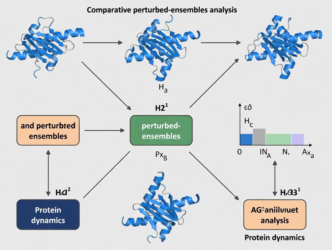
Comparative Perturbed-Ensembles Analysis: Decoding Functional Protein Dynamics for Drug Discovery
This article explores Comparative Perturbed-Ensembles Analysis, a powerful computational approach that compares conformational ensembles from molecular dynamics simulations under different perturbations to reveal functional protein dynamics.
Comparative Perturbed-Ensembles Analysis: Decoding Functional Protein Dynamics for Drug Discovery
Abstract
This article explores Comparative Perturbed-Ensembles Analysis, a powerful computational approach that compares conformational ensembles from molecular dynamics simulations under different perturbations to reveal functional protein dynamics. Aimed at researchers, scientists, and drug development professionals, we cover the foundational shift from static to dynamic structure paradigms, detailed methodologies for implementing the analysis, strategies to overcome computational and analytical challenges, and rigorous validation against experimental data. By synthesizing insights from recent advances in AI structure prediction and ensemble analysis tools, this guide provides a comprehensive resource for leveraging protein dynamics to understand allosteric mechanisms and accelerate the development of conformation-specific therapeutics.
From Static Structures to Dynamic Ensembles: The Paradigm Shift in Protein Science
Proteins are not static, rigid structures; they are inherently dynamic molecules whose functional motions—from loop rearrangements to secondary structure shifts—play pivotal roles in virtually all biological processes, including catalysis, signaling, and molecular interactions [1]. These conformational changes, often occurring on microsecond or slower timescales, are governed by an energy landscape that dictates the populations and interconversion rates of discrete states [1]. The time dependence of biomolecular structural changes remains underexplored yet is essential for defining the roles of transient states and dynamically driven allostery in protein function. Traditional static structural methods, such as X-ray crystallography, provide invaluable but limited snapshots of this complex dynamical repertoire. This application note explores the framework of comparative perturbed-ensembles analysis, a powerful approach for detecting functional dynamics in proteins, and details contemporary protocols and tools enabling this research within drug discovery and biotechnology contexts.
Comparative Perturbed-Ensembles Analysis: A Core Analytical Framework
The central challenge in molecular dynamics (MD) simulation lies not just in sampling the conformational energy landscape but in analyzing the resulting trajectories to extract biologically relevant information. The comparative perturbed-ensembles analysis approach addresses this by systematically comparing two or more conformational ensembles of a system generated by MD simulations under distinct perturbation conditions [2].
In this framework, perturbations can include different sequence variations (e.g., single-point mutations), ligand-binding conditions, post-translational modifications, or other physical/chemical modifications. Each simulation must be sufficiently long (e.g., microsecond-long) to ensure adequate sampling of local substates. Subsequently, sophisticated bioinformatic and statistical tools are applied to extract function-related information, including:
- Principal component analysis (PCA) to identify essential dynamics
- Residue-residue contact analysis
- Difference contact network analysis (dCNA) based on graph theory
- Statistical analysis of side-chain conformations [2]
By comparing distinct conformational ensembles, functional micro- to millisecond dynamics can be inferred—a timescale difficult to reach in a single simulation and even more challenging to link to specific functions without comparative analysis [2]. The workflow of this approach is illustrated in Diagram 1.
Diagram 1: Workflow of Comparative Perturbed-Ensembles Analysis
Applications and Validation
This approach has been successfully implemented to identify allosteric pathways in cyclophilin A (CypA), revealing two pathways consistent with NMR experiments and a novel third pathway [2]. It has further enabled dynamical-evolution analysis across human cyclophilin isoforms (CypA, CypD, and CypE), identifying both conserved and divergent conformational dynamics [2]. Computational findings from this approach require validation with experimental data, creating a closed loop of hypothesis generation and testing that significantly enhances the reliability of the functional dynamics detected.
Quantitative Benchmarks for Protein Dynamics Methodologies
The field of protein dynamics simulation employs diverse methodologies, each with distinct strengths, limitations, and performance characteristics. The table below summarizes key quantitative benchmarks for current technologies:
Table 1: Performance Comparison of Protein Dynamics Analysis Methods
| Method | Timescale | Spatial Resolution | Throughput | Key Applications | Sample Requirements |
|---|---|---|---|---|---|
| Molecular Dynamics (MD) [3] [4] | Nanoseconds to milliseconds | Atomic (~1-3 Å) | Low (months on supercomputers) | Folding/unfolding pathways, allosteric mechanisms | Computational resources intensive |
| Comparative Perturbed-Ensembles MD [2] | Microseconds to milliseconds | Atomic (~1-3 Å) | Medium (multiple μs-length simulations) | Allosteric pathway identification, functional dynamics | Requires multiple simulation conditions |
| BioEmu (AI) [4] | Equilibrium ensembles | Atomic (backbone frames) | Very High (1000s structures/hour on single GPU) | Genome-scale function prediction, cryptic pocket discovery | Single protein sequence; minimal compute |
| 2DIR with ML [5] | Picoseconds to milliseconds | Backbone (Cα RMSD ~2.5-3.3 Å) | Medium (theoretical spectra generation) | Folding trajectories, unknown protein structure prediction | Experimental or theoretical 2DIR spectra |
| Stopped-Flow EPR [1] | Milliseconds | Nanoscale (spin label distances) | Low (stopped-flow measurements) | Folding pathways, allosteric changes in membrane proteins | 10-100 μg of spin-labeled protein |
These methodologies represent complementary approaches, with traditional MD simulations offering high spatial resolution but limited timescales, while emerging AI-based methods like BioEmu dramatically accelerate the sampling of equilibrium ensembles with approximately 1 kcal/mol accuracy [4]. Experimental techniques like 2DIR spectroscopy and stopped-flow EPR provide crucial experimental validation, with the latter enabling investigation of complex, biologically relevant proteins that are often only available in limited quantities [5] [1].
Experimental Protocols for Dynamic Analysis
Protocol 1: Comparative Perturbed-Ensembles MD Analysis
This protocol outlines the procedure for implementing comparative perturbed-ensembles analysis using molecular dynamics simulations [2].
4.1.1 System Preparation and Perturbation Design
- Select a protein system of interest and identify perturbation conditions relevant to biological function (e.g., wild-type vs. mutant, apo vs. holo forms, different ligand-binding states, post-translational modifications)
- Obtain initial coordinates from the Protein Data Bank (PDB) and add missing atoms using standard software tools
- For each perturbation condition, prepare separate simulation systems with identical setup aside from the introduced perturbation
4.1.2 Molecular Dynamics Simulations
- Solvate each system in explicit water using the experimental water density for the temperature of interest
- Employ energy minimization to remove steric clashes, followed by gradual heating and equilibration phases
- Production simulations:
- Perform microsecond-length simulations for each perturbation condition (current benchmarks suggest ≥1 μs)
- Use a fully flexible force field with explicit water representation
- Maintain constant temperature and pressure using appropriate thermostats and barostats
- Save trajectories at sufficient frequency (e.g., every 100 ps) to capture relevant dynamics
4.1.3 Comparative Ensemble Analysis
- Align all trajectories to a reference structure to remove global rotation and translation
- Perform principal component analysis (PCA) to identify essential collective motions:
- Construct and diagonalize the covariance matrix of atomic positional fluctuations
- Compare the projection of each ensemble onto the principal components
- Conduct residue-residue contact analysis using a distance cutoff (e.g., 4.5 Å for heavy atoms)
- Implement difference contact network analysis (dCNA):
- Construct graphs where nodes represent residues and edges represent persistent contacts
- Identify differences in network connectivity between ensembles
- Analyze side-chain torsion-angle distributions to identify significant conformational changes
4.1.4 Validation and Interpretation
- Compare computational findings with available experimental data (NMR, EPR, etc.)
- Identify statistically significant differences between ensembles (e.g., using Kolmogorov-Smirnov tests for distribution comparisons)
- Map identified dynamic pathways and allosteric networks onto protein structure for functional interpretation
Protocol 2: AI-Enhanced Equilibrium Ensemble Generation with BioEmu
BioEmu represents a transformative AI-based approach for generating protein equilibrium ensembles, offering dramatic speed improvements over traditional MD [4].
4.2.1 Input Preparation and Model Configuration
- Input requirement: Protein amino acid sequence (single-chain proteins up to ~500 residues)
- Hardware requirement: Single GPU (recommended) or CPU alternative
- Install BioEmu package and dependencies as specified in the original implementation
- Configure model parameters based on desired trade-off between sampling speed and accuracy
4.2.2 Ensemble Generation Process
- Encode the input sequence using the Evoformer module from AlphaFold2 to generate single and pairwise representations
- Feed representations into the diffusion-based denoising model, which uses coarse-grained backbone frames
- Generate structural samples through 30-50 denoising steps, producing thousands of structures per hour on a single GPU
- For thermodynamic accuracy, employ Property Prediction Fine-Tuning (PPFT) if experimental stability data (e.g., melting temperature) is available
4.2.3 Analysis of Generated Ensembles
- Cluster generated structures to identify predominant conformational states
- Calculate free energy differences between states using Boltzmann distributions
- Identify cryptic pockets by analyzing surface accessibility across the ensemble
- Compare with experimental structures (e.g., from PDB) using RMSD metrics (target: ≤3 Å for domain motions)
Protocol 3: Machine Learning-Enabled 2DIR Spectroscopy for Dynamic Structures
This protocol details the procedure for predicting dynamic protein structures from two-dimensional infrared (2DIR) spectroscopy using machine learning [5].
4.3.1 Data Preparation and Spectral Generation
- Curate a diverse set of protein structures (up to 100 residues for initial training) from RCSB PDB and SWISS-PROT
- Generate theoretical 2DIR spectra for each protein conformation:
- Use the Frenkel exciton Hamiltonian within the amide I spectral window (1,575 to 1,725 cm⁻¹)
- Apply vibrational spectroscopic maps parameterized against experimental findings
- Calculate corresponding Cα distance maps as ground truth for ML training
- Convert 2DIR signals into standardized 3 × 224 × 224 RGB images for model input
4.3.2 Model Training and Validation
- Implement DeepLabV3 architecture for image segmentation to distance map prediction
- Configure model with:
- Feature extraction layers with atrous convolutions for multiscale context
- Upsampling path with skip connections to restore spatial dimensions
- MaskLoss function to handle variable protein sizes via padding
- Train model using Adam optimizer with batch normalization for stabilization
- Validate using k-fold cross-validation with metrics including:
- Mean Absolute Error (MAE) for distance maps (target: ~2.20 Å)
- Long-range precision (Top-L/5, Top-L/2, Top-L)
- Cα RMSD for final 3D structures (target: ~2.54 Å)
4.3.3 Prediction of Dynamic Structures
- For experimental applications, collect 2DIR spectra of the protein under study
- Preprocess experimental spectra to match training data format
- Apply trained model to predict Cα distance maps from input spectra
- Reconstruct 3D backbone structures using gradient-based folding algorithm
- Analyze folding trajectories by applying the protocol to time-resolved 2DIR data
Signaling Pathway Dynamics: Allosteric Regulation
Proteins often employ allosteric mechanisms to regulate their function, where a perturbation at one site (e.g., ligand binding or mutation) dynamically influences a distal functional site. The comparative perturbed-ensembles approach has been instrumental in elucidating these mechanisms, as demonstrated in studies of cyclophilin A and other systems [2]. Diagram 2 illustrates a generalized allosteric signaling pathway in a protein, highlighting the dynamic propagation of structural changes.
Diagram 2: Dynamic Allosteric Signaling Pathways in Proteins
Successful implementation of protein dynamics studies requires specific computational and experimental resources. The table below details key research reagent solutions for the featured methodologies.
Table 2: Research Reagent Solutions for Protein Dynamics Analysis
| Resource Name | Type | Primary Function | Key Features | Access Information |
|---|---|---|---|---|
| Dynameomics Database [3] | Data Resource | Repository of native state and unfolding simulation data | Contains ~200 μs of simulation data for >1000 proteins representing majority of globular folds | Publicly accessible at www.dynameomics.org |
| Comparative Perturbed-Ensembles Analysis [2] | Analytical Approach | Compare MD ensembles under different conditions | Identifies function-related dynamics through systematic comparison of perturbation states | Protocol detailed in Application Note Section 4.1 |
| BioEmu [4] | AI Software | Generate protein equilibrium ensembles | 4-5 orders of magnitude speedup vs MD; ~1 kcal/mol accuracy on single GPU | Implementation details in Lewis et al., Science 2025 |
| 2DIR-ML Protocol [5] | Analytical Protocol | Predict 3D structures from 2D IR spectra | Establishes "spectrum-structure" relationship; captures μs-ms dynamics | DeepLabV3-based model as described in PNAS 2025 |
| High-Sensitivity Stopped-Flow EPR [1] | Instrumentation | Monitor millisecond conformational kinetics | Custom dielectric resonator; minimized sample waste; 10-100 μg protein requirement | Technical specifications in Protein Science article |
| ilmm (in lucem molecular mechanics) [3] | MD Software | Perform molecular dynamics simulations | Fully flexible force field parameters; F3C water model | Development version used in Dynameomics project |
The integration of comparative perturbed-ensembles analysis with emerging AI technologies and advanced experimental methods represents a paradigm shift in protein science. By moving beyond static snapshots to embrace the intrinsically dynamic nature of proteins, researchers can uncover deeper insights into allosteric mechanisms, conformational landscapes, and functional dynamics. These approaches are already accelerating drug discovery by revealing cryptic pockets and enabling genome-scale dynamics predictions. As these methodologies continue to evolve and integrate, they promise to transform our understanding of protein function and open new avenues for therapeutic intervention.
The classical sequence-structure-function paradigm, which dominated twentieth-century molecular biology, tacitly stipulated that a single, well-defined three-dimensional structure governs a protein's function [6]. While foundational, this view is insufficient for describing the mechanisms that sustain cell life. Modern molecular biology now recognizes that function requires proteins to exist in more than a single structure, to switch between these structures, and for these structures to be incompletely organized [6]. This recognition has necessitated an updated sequence-conformational ensemble-function paradigm, with the powerful energy landscape concept as its foundation [6].
This framework embraces the reality that proteins are dynamic systems, constantly interconverting between conformational states with varying energies, where the relative stability of a conformation dictates its population within the ensemble [6]. The changes in the populations of these states—driven by interactions with ligands, membranes, other proteins, or through mutations—are fundamental to biological activity and cellular regulation [6]. Understanding these core principles is essential for comparative perturbed-ensembles analysis, a research approach that systematically compares these dynamic ensembles under different conditions to decipher functional mechanisms and dysfunction.
Core Principles and Definitions
The Conformational Ensemble
A protein does not possess a single rigid structure but exists as a collection of interconverting conformations, known as a conformational ensemble [6]. The powerful energy landscape idea, imported from physics and chemistry, forms the foundation for this modern understanding [6]. The ensemble includes the ground state (often the lowest energy, most populated conformation) as well as multiple higher-energy, less populated states. The relative propensities of these states, rather than a single rigid structure, are the true hallmark of cell life [6].
The Energy Landscape
The energy landscape is a multidimensional surface that maps all possible conformations of a protein and their associated energies [6] [7]. It describes the choreography of protein folding and dynamics.
- Energy Minima (Wells): Represent metastable conformational states. The depth of a minimum corresponds to the thermodynamic stability of that state [7].
- Energy Barriers (Peaks): Separate different conformational states. The height of a barrier dictates the kinetic stability—how readily the protein can transition from one state to another [7].
- Basin of Attraction: The region of the landscape surrounding a minimum; a protein within this basin will relax to that stable state.
The sequence of a functional protein is evolutionarily selected to create a "rough" energy landscape with multiple minima, which correlates with frustration in folding. This roughness is not a flaw but a functional necessity, enabling conformational malleability for binding-induced folding and allosteric regulation [7].
Functional States and Population Shifts
Functional properties like activation, inhibition, and allosteric regulation are governed by shifts in the populations of states within the conformational ensemble [6]. Under physiological conditions, proteins often predominantly populate their inactive conformations, with the active state representing only a minor population [6]. Function is triggered when effectors, the membrane, or oncogenic mutations stabilize the active state, increasing its population and driving a bistable switch [6]. The number of molecules in the active state ultimately determines protein function [6]. Allostery, the process by which binding at one site influences activity at a distant site, is a hallmark of this population-based regulation [6].
Quantitative Characterization of Ensembles and Landscapes
Experimental and computational methods are used to quantify the features of energy landscapes and the properties of conformational ensembles. The table below summarizes key parameters and the techniques used to measure them.
Table 1: Quantitative Parameters for Characterizing Conformational Ensembles and Energy Landscapes
| Parameter | Description | Experimental/Computational Methods |
|---|---|---|
| State Populations | The relative proportion of a specific conformation within the ensemble. | Markov Models from single-molecule data [8], NMR, Time-resolved cryo-EM [9]. |
| Transition Rates | The kinetic rate constants for interconversion between two conformational states. | Single-molecule techniques (e.g., NOTs) analyzed with Kramers' theory [8], MD simulations [10]. |
| Free Energy (ΔG) | The relative stability difference between two conformational states. | Inferred from state populations in single-molecule experiments (ΔG = -kT ln(PA/PB)) [8]. |
| Activation Energy (Ea) | The height of the energy barrier separating two states, determining transition kinetics. | Derived from temperature-dependent transition rates using Arrhenius or Kramers' theory [8]. |
| Entropy Change (ΔS) | The change in conformational disorder during a state transition. | Calculated from temperature-dependent free energy measurements (ΔG = ΔH - TΔS) [8]. |
| Molecular Polarizability | A measure of how a protein's electron cloud distorts in an electric field, reporting on structural changes. | Calculated from atomistic models and correlated with transmission signals in nanoaperture optical tweezers [8]. |
The following workflow illustrates the general process for mapping a protein's energy landscape from experimental data, as demonstrated in single-molecule studies:
Experimental Protocols for Ensemble Analysis
Protocol: Mapping Energy Landscapes with Nanoaperture Optical Tweezers (NOTs)
This protocol details the procedure for using NOTs to resolve the energy landscape of a single, unmodified protein, as demonstrated for Bovine Serum Albumin (BSA) [8].
I. Principle NOTs trap a single protein without the need for fluorescent labels or tethers. Conformational changes alter the protein's polarizability, which is detected as changes in the transmission intensity of the laser beam through the nanoaperture. This allows for direct, label-free observation of state transitions and the calculation of the underlying energy landscape [8].
II. Materials and Reagents
- Protein of Interest: Purified, e.g., Bovine Serum Albumin (BSA).
- Buffers: Appropriate physiological buffer at neutral pH for initial measurements.
- Nanoaperture Substrate: A chip fabricated with double nanoholes (DNH).
- Nanoaperture Optical Tweezer Setup: Consisting of:
- Laser source (e.g., 980 nm).
- Microscope objective for trapping and signal collection.
- Avalanche Photodiode (APD) for high-sensitivity transmission detection.
- Temperature control system (often via laser power modulation with pre-calibrated local heating).
III. Procedure
- Sample Preparation: Dilute the protein to a low concentration (pM-nM) in the desired buffer to ensure single-molecule trapping events.
- System Calibration:
- Calibrate the system using polystyrene nanoparticles of known size to establish a baseline signal and confirm the absence of discrete state transitions.
- Correlate specific transmission signal levels with known protein conformations, if available (e.g., for BSA, the N-state at neutral pH and F-state at low pH).
- Data Acquisition:
- Flow the protein solution over the DNH chip.
- Initiate trapping with the laser and record the transmission signal at a high sampling rate (e.g., 100 kHz) for an extended period.
- Systematically vary the local temperature by adjusting the laser power to probe temperature-dependent dynamics.
- Data Analysis:
- State Identification: Identify discrete conformational states from the step-like changes in the transmission time-series data.
- Point Spread Function (PSF) Deconvolution: Account for signal broadening due to translational/rotational motion and noise by deconvolving a predetermined PSF from the raw data.
- Probability Density Function (PDF): Generate a binned histogram of the deconvolved transmission signal to obtain the PDF.
- Energy Landscape Calculation: Calculate the free energy landscape using the relationship ( G = -k_B T \ln(P(V)) ), where ( P(V) ) is the PDF and ( V ) is the signal coordinate.
- Kinetic Modeling: Model the state transition dynamics using a Markov model and fit the transition rates with Kramers' theory to extract thermodynamic parameters (e.g., activation energy, entropy changes).
Protocol: The Relaxed Complex Scheme for Drug Discovery
This protocol outlines the Relaxed Complex Method (RCM), a computational strategy that integrates protein dynamics from Molecular Dynamics (MD) simulations into structure-based drug discovery [11].
I. Principle The RCM addresses the limitation of traditional docking, which often uses a single, static protein structure. It recognizes that binding involves selection from a pre-existing ensemble of conformations. By docking compound libraries into multiple representative snapshots (including cryptic pockets) from an MD trajectory, the RCM increases the probability of identifying hits that leverage protein flexibility for high-affinity binding [11].
II. Materials and Software
- Protein Structure: A high-resolution starting structure (from crystallography, cryo-EM, or AlphaFold2 prediction).
- MD Software: GROMACS, AMBER, or DESMOND [10].
- Molecular Docking Software: Any standard docking program (e.g., AutoDock Vina, Glide).
- Compound Library: A virtual library of drug-like molecules (e.g., ZINC, Enamine REAL Database) [11].
- High-Performance Computing (HPC) Cluster: With adequate CPU/GPU resources.
III. Procedure
- System Preparation:
- Prepare the protein structure (adding missing atoms, protonation states) and solvate it in a water box with appropriate ions.
- Molecular Dynamics Simulation:
- Perform an MD simulation of the target protein (apo or in a relevant state) for a timescale sufficient to capture functionally relevant motions (nanoseconds to microseconds).
- Ensure simulation stability by monitoring root-mean-square deviation (RMSD).
- Trajectory Clustering and Snapshot Selection:
- Cluster the MD trajectory based on structural similarity (e.g., using RMSD on the binding site residues).
- Select a set of representative snapshot structures from the major clusters, ensuring conformational diversity.
- Molecular Docking:
- Prepare the selected protein snapshots and the ligand library for docking.
- Perform molecular docking of the entire ligand library against each representative protein snapshot.
- Hit Identification and Analysis:
- Consolidate and rank the docking results from all snapshots based on scoring functions (e.g., binding affinity).
- Analyze top-ranking hits for consistent binding modes across multiple snapshots or for specific stabilization of a particular functional conformation (e.g., DFG-in vs. DFG-out in kinases).
The following diagram illustrates the logical flow of the RCM and its key advantage over static docking:
The Scientist's Toolkit: Key Research Reagents and Solutions
The following table details essential materials, software, and reagents used in the experimental and computational protocols featured in this note.
Table 2: Research Reagent Solutions for Conformational Ensemble Studies
| Item Name | Function/Application | Example Specifications/Products |
|---|---|---|
| Nanoaperture Substrate | Creates a highly confined optical trap to immobilize a single protein for label-free detection of conformational changes. | Double Nanohole (DNH) fabricated in a gold film [8]. |
| Bovine Serum Albumin (BSA) | A canonical model protein for method development and validation in single-molecule biophysics studies. | 66 kDa, water-soluble monomer; commercial purity >98% [8]. |
| MD Force Fields | Empirical potential functions defining interatomic interactions; critical for the accuracy of MD simulations. | CHARMM, AMBER, OPLS-AA [10]. |
| MD Simulation Software | Software suites to perform and analyze all-atom MD simulations of biomolecules. | GROMACS, AMBER, DESMOND [10]. |
| Ultra-Large Virtual Libraries | Source of billions of synthesizable compounds for virtual screening against dynamic targets. | Enamine REAL Database, Synthetically Accessible Virtual Inventory (SAVI) [11]. |
| AlphaFold2 | AI tool for highly accurate protein structure prediction from sequence; provides models for targets without experimental structures. | AlphaFold Protein Structure Database [11] [12]. |
| Generative AI Models for SBDD | De novo design of drug-like molecules considering protein flexibility and conformational changes. | DynamicFlow, other deep generative models [13]. |
| Time-Resolved Cryo-EM | Captures high-resolution snapshots of biomolecular machines in action, visualizing rare intermediate states. | Advanced cryo-electron microscopes with rapid plunge-freezing or microfluidics [9]. |
Defining Comparative Perturbed-Ensembles Analysis and its Core Hypothesis
Comparative Perturbed-Ensembles Analysis (CPEA) is a computational structural biology framework for quantifying changes in protein energy landscapes induced by perturbations such as ligand binding, mutations, or post-translational modifications. The methodology operates on the fundamental principle that proteins exist as ensembles of interconverting conformations, and that functional regulation often occurs through population shifts within these ensembles rather than through single, static structural changes [14].
The core hypothesis of CPEA posits that a precise comparison of conformational ensembles—between a reference state (e.g., apo protein) and a perturbed state (e.g., holo, phosphorylated, or mutated protein)—can reveal functionally relevant changes in structure and dynamics that are invisible to static structural comparisons. This hypothesis is formalized through its connection to thermodynamics; the measure used to compare ensembles, the Kullback-Leibler Divergence, is fundamentally a measure of the free energy difference between the two equilibrium ensembles [14]. This provides CPEA with a strong thermodynamic foundation that distinguishes it from simple geometric comparisons.
Key Applications in Protein Research
CPEA is particularly powerful for investigating complex biological phenomena where changes in dynamics are as critical as changes in structure.
- Allosteric Regulation: CPEA can identify changes in conformational distributions and dynamics at sites distant from the location of a perturbation, such as a ligand-binding event or a point mutation [14]. This allows for an unbiased discovery of allosteric networks.
- Post-Translational Modification (PTM) Effects: Systematically assessing the structural consequences of phosphorylation, as demonstrated in a global analysis of phosphorylated protein structures, which revealed that phosphorylation tends to induce small, stabilizing conformational changes and modulate protein dynamics [15].
- Drug Binding and Resistance: Understanding how mutations, particularly those conferring drug resistance, modulate ligand binding by altering the protein's energy landscape and conformational dynamics [14].
- Functional Site Identification: CPEA can help identify key functional residues by pinpointing regions where artificial perturbations cause large changes in the conformational ensemble, as these sites often co-localize with functional epitopes [14].
Quantitative Data from Perturbed-Ensemble Studies
Table 1: Quantitative Findings from a Global Analysis of Phosphorylation-Induced Structural Changes [15]
| Analysis Metric | Finding | Implication |
|---|---|---|
| Global Backbone RMSD | Median change: 1.14 ± 3.13 Å; Only 28.14% of phosphosites showed changes ≥ 2 Å. | Phosphorylation typically induces subtle conformational changes rather than large rearrangements. |
| Structural Uniformity | Median RMSD among phosphorylated structures is smaller than among non-phosphorylated counterparts. | Phosphorylation often stabilizes a particular backbone conformation, reducing structural heterogeneity. |
| Protein Kinase Domains | Median phosphorylation-induced RMSD: 1.51 Å (vs. 0.73 Å for rest of dataset). | Kinases undergo larger conformational changes upon phosphorylation, consistent with their regulatory mechanisms. |
Table 2: Key Metrics for Comparing Conformational Ensembles Using the Kullback-Leibler Divergence (KLD) [14]
| Metric/Parameter | Description | Role in CPEA |
|---|---|---|
| First-Order KLD Terms | KLD calculated for individual torsion angles (φ, ψ, χ). | Captures local population shifts and changes in flexibility at the single-residue level. |
| Second/Higher-Order KLD Terms | KLD calculated for pairs (or more) of correlated degrees of freedom. | Identifies coordinated changes and allosteric coupling between residues. |
| Mutual Divergence | Analogous to mutual information, but uses relative entropy. | Quantifies the co-dependence of conformational changes between two residues upon perturbation. |
Experimental and Computational Protocols
Protocol 1: CPEA Using Molecular Dynamics Simulations and Kullback-Leibler Divergence
This protocol is adapted from the methodology implemented in the MutInf software package [14].
1. Ensemble Generation:
- System Preparation: Create atomic-level structures for both the reference (e.g., apo protein) and perturbed (e.g., ligand-bound, mutated) systems.
- Molecular Dynamics (MD) Simulation: Perform multiple, independent MD simulations for each state to generate conformational ensembles. Ensure simulations are sufficiently long to achieve adequate sampling of relevant states. Save molecular snapshots at regular intervals (e.g., every 100 ps) for subsequent analysis.
2. Torsion Angle Space Transformation:
- Coordinate Extraction: For each saved snapshot, extract the backbone (φ, ψ) and side-chain (χ₁, χ₂, ...) torsion angles for all residues. The use of internal torsion coordinates avoids frame-fitting issues inherent in Cartesian coordinate analysis [14].
- Probability Density Estimation: Construct discrete probability distributions for each torsion angle in both the reference and perturbed ensembles. This is typically done by histogramming the torsion angle values over the entire simulation trajectory.
3. Kullback-Leibler Divergence Calculation:
- First-Order (Local) Analysis: Calculate the KLD for each individual torsion angle using the formula:
KLD = Σ [ρ(x) * ln(ρ(x) / ρ*(x))]whereρ(x)is the probability distribution of the perturbed ensemble andρ*(x)is the distribution of the reference ensemble [14]. - Statistical Filtering: Use bootstrap resampling to estimate the statistical significance of the calculated KLD values. Filter out results that are not statistically significant to ensure a low-background, high-signal analysis [14].
- Higher-Order (Correlated) Analysis (Optional): Calculate second-order KLD terms for pairs of torsion angles (e.g., within a residue or between interacting residues) to capture correlated motions using the Generalized Kirkwood Superposition Approximation [14].
4. Visualization and Interpretation:
- Residue-Level Mapping: Map the significant first-order KLD values for all torsions of a residue onto the protein structure, often creating a visualization where color intensity on the structure corresponds to the magnitude of the ensemble change.
- Identification of Allosteric Sites: Residues displaying high KLD values distal to the perturbation site are candidate allosteric residues.
Protocol 2: CPEA Using Experimental Structural Ensembles with EnsembleFlex
This protocol utilizes the EnsembleFlex computational suite for analyzing experimentally derived structural ensembles from the PDB (e.g., from X-ray crystallography, NMR, or cryo-EM) [16].
1. Data Curation and Superposition:
- Ensemble Collection: Compile a set of PDB structures for the protein in its reference and perturbed states. This may include multiple crystal forms, NMR models, or structures with and without a post-translational modification like phosphorylation [15].
- Structural Alignment: Superimpose all structures (both reference and perturbed) onto a common reference frame, typically using a conserved, rigid core of the protein to avoid bias [16].
2. Flexibility and Variability Analysis:
- Backbone Flexibility: Calculate per-residue Root-Mean-Square Fluctuation (RMSF) for the backbone atoms (Cα) within each ensemble to quantify flexibility [16].
- Side-Chain Conformational Heterogeneity: Analyze the rotameric states and spatial occupancy of side chains to identify residues with significant population shifts between ensembles.
- Principal Component Analysis (PCA): Perform PCA on the combined set of superposed structures. This reduces the dimensionality of the conformational data to identify the dominant collective motions that distinguish the reference and perturbed ensembles [16].
3. Binding-Site and Conservation Analysis:
- Ligand-Site Variability Mapping: If applicable, automatically map the variability of binding-site geometries across the ensemble [16].
- Conserved Water Identification: Identify structurally conserved water molecules within the ensembles, as these can be critical for function and their displacement can signal important ensemble shifts [16].
4. Comparative Quantification:
- State Identification: Use clustering algorithms on the principal components to identify distinct conformational states and quantify their populations in the reference versus perturbed ensembles [16].
- Statistical Testing: Perform statistical tests (e.g., Mann-Whitney U test) to rigorously assess whether observed differences in RMSF, state populations, or other metrics are significant [15].
Signaling Pathway and Workflow Visualization
The following diagram illustrates the logical workflow and data flow for a typical Comparative Perturbed-Ensembles Analysis, integrating both simulation and experimental approaches.
CPEA Core Workflow
The Scientist's Toolkit: Research Reagent Solutions
Table 3: Essential Software and Data Resources for CPEA
| Tool/Resource | Type | Primary Function in CPEA | Reference |
|---|---|---|---|
| MutInf | Software Package | Calculates the Kullback-Leibler Divergence between conformational ensembles from MD simulations to identify population shifts. | [14] |
| EnsembleFlex | Computational Suite | Performs integrated analysis of experimental structural ensembles (X-ray, NMR, cryo-EM) for flexibility, clustering, and binding-site variability. | [16] |
| CPDB (Protein Data Bank) | Database | Primary repository for experimentally solved protein structures, used as a source for building reference and perturbed ensembles. | [15] |
| GROMACS/AMBER | MD Simulation Engine | Generates conformational ensembles through atomic-level molecular dynamics simulations. | [14] |
| Climateprediction.net (CPDN) | Computing Platform | A distributed computing project that runs large perturbed-parameter ensembles; a conceptual model for large-scale ensemble simulation in biology. | [17] |
Proteins are inherently dynamic molecules that exist as an ensemble of interconverting conformations rather than single, static structures. This conformational heterogeneity is a fundamental determinant of protein function, enabling mechanisms such as allostery, catalysis, and signal transduction. The dynamic nature of proteins arises from two primary sources: intrinsic dynamics governed by the protein's amino acid sequence and energy landscape, and external perturbations induced by environmental factors, ligand binding, or cellular interactions. Understanding these conformational ensembles is crucial for advancing fundamental biology and accelerating drug discovery efforts, particularly for targeting proteins with significant structural flexibility, including many challenging drug targets.
Recent breakthroughs in artificial intelligence, particularly AlphaFold, have revolutionized static structure prediction but face limitations in capturing the full spectrum of protein dynamics [18] [19]. This application note provides a comprehensive overview of contemporary methodologies for studying conformational heterogeneity, presenting quantitative comparisons, detailed experimental protocols, and essential computational tools for researchers investigating protein dynamics.
Quantitative Comparison of Methodologies
The study of conformational ensembles employs diverse computational and experimental approaches, each with distinct strengths, limitations, and applicable resolution ranges. The table below summarizes key quantitative metrics for major methodologies discussed in this application note.
Table 1: Quantitative Comparison of Methodologies for Studying Conformational Heterogeneity
| Method | Spatial Resolution | Temporal Resolution | Key Measurable Parameters | Throughput | Information Gained |
|---|---|---|---|---|---|
| FiveFold [18] | Atomic (Cα) | Thermodynamic states | PFSC strings, conformational clusters | High | Complete folding space for 5-residue fragments, massive conformational ensembles |
| DIRseq [20] | Single residue | Binding equilibrium | Drug-interacting residue propensity | Very High | Sequence-based prediction of drug-binding residues in IDPs |
| MD-NMR Integration [21] | Atomic | ps-ms | R1, R2, NOE, ηxy rates, order parameters (S²) | Low | Atomistic dynamics, time-resolved 4D conformational ensembles |
| AI-2DIR Spectroscopy [5] | Atomic (Cα backbone) | μs-ms | Cα distance maps, RMSD (2.54 Å average) | Medium | Dynamic folding trajectories, static structures of uncharacterized proteins |
| ProFlex (NMA) [22] | Cα coarse-grained | Harmonic motions | RMSF profiles, flexibility alphabets | Very High | Global flexibility trends, relative dynamics across structural database |
| EnsembleFlex [16] | Backbone & side-chain | Structural snapshots | RMSD/RMSF, PCA/UMAP clusters, binding site variability | High | Conformational heterogeneity from experimental PDB ensembles |
Research Reagent Solutions Toolkit
Implementing conformational ensemble studies requires specialized computational tools and resources. The following table catalogizes essential research reagents and their applications in perturbed-ensemble analysis.
Table 2: Essential Research Reagents and Computational Tools for Ensemble Analysis
| Tool/Resource | Type | Primary Function | Access |
|---|---|---|---|
| FiveFold [18] | Algorithm & Web Server | Generates massive conformational ensembles using PFSC/PFVM | Web server |
| DIRseq [20] | Prediction Server | Identifies drug-interacting residues in disordered proteins from sequence | https://zhougroup-uic.github.io/DIRseq/ |
| EnsembleFlex [16] | Analysis Suite | Quantifies conformational heterogeneity from experimental PDB ensembles | Open access |
| ProFlex Toolkit [22] | Flexibility Analysis | Encodes protein flexibility into alphabetic representations for large-scale analysis | Available with publication |
| SwissDock 2024 [20] | Docking Server | Small-molecule docking with Attracting Cavities and AutoDock Vina | Web server |
| PDB-PFSC Database [18] | Structural Database | Repository of protein structures converted to PFSC strings | Database |
| 5AAPFSC Database [18] | Conformational Database | All possible folding patterns for five amino acid fragments | Database |
Experimental Protocols
Protocol: FiveFold Conformational Ensemble Prediction
The FiveFold approach addresses limitations of single-state predictions by generating comprehensive conformational ensembles based on local folding principles [18].
Materials:
- Protein amino acid sequence
- FiveFold software suite or web server
- PDB-PFSC database
- 5AAPFSC database (3.2 million five-amino-acid permutations)
Procedure:
- PFSC Assignment: Convert the input protein sequence into Protein Folding Shape Code (PFSC) strings using the 27-letter alphabet representing all possible five-residue folding patterns.
- PFVM Construction: Assemble the Protein Folding Variation Matrix (PFVM) to map local folding variations along the entire sequence, revealing intrinsic fluctuation patterns.
- Conformational Sampling: Generate a massive number of possible PFSC strings through optimized combinations of local folding patterns from the PFVM.
- Structure Assembly: Screen the PDB-PFSC database using generated PFSC strings to identify and retrieve compatible structural fragments.
- Ensemble Construction: Assemble complete 3D structures from compatible fragments, generating the final conformational ensemble for analysis.
Applications: Intrinsically disordered proteins, mutational analysis, folding pathway studies, and alternative conformation prediction.
Protocol: Integrative MD-NMR Ensemble Validation
This protocol combines molecular dynamics simulations with NMR relaxation data to generate and validate biologically relevant conformational ensembles [21].
Materials:
- AlphaFold-predicted protein structure or experimental structure
- High-performance computing resources for MD simulations
- NMR spectrometer (≥600 MHz)
- Isotopically labeled protein (¹⁵N, ¹³C)
- NMR data processing software (NMRPipe, CCPN)
- MD simulation software (AMBER, GROMACS, CHARMM)
- Back-calculation and analysis scripts (ABSURDer, MaxEnt)
Procedure:
- Initial Structure Preparation: Obtain starting structure from AlphaFold prediction or experimental determination. Perform energy minimization and solvation.
- MD Simulation: Conduct extensive free MD simulations (≥1 μs) using modern force fields (AMBER, CHARMM). Maintain physiological conditions (temperature, pH, ionic strength).
- NMR Data Acquisition: Collect ¹⁵N relaxation data (R₁, R₂, heteronuclear NOE) and cross-correlated relaxation (ηxy) rates using optimized pulse sequences.
- Trajectory Segmentation: Divide MD trajectory into segments based on RMSD plateaus, identifying structurally stable regions.
- Parameter Back-Calculation: Compute theoretical NMR relaxation parameters (R₁, R₂, NOE, ηxy) from each MD trajectory segment.
- Ensemble Selection: Identify trajectory segments where back-calculated parameters match experimental NMR data within acceptable error margins (χ² minimization).
- Validation: Analyze selected ensembles for functional relevance, particularly in flexible regions with biological significance.
Applications: Validation of dynamic ensembles, identification of functional conformational states, characterization of allosteric mechanisms.
Protocol: AI-Enhanced 2DIR Spectroscopy for Dynamic Structure Prediction
This innovative protocol combines two-dimensional infrared spectroscopy with machine learning to predict dynamic protein structures in real-time [5].
Materials:
- Protein sample (natural or isotopic labeling)
- 2DIR spectrometer with femtosecond laser system
- Curated protein structure database (RCSB PDB, SWISS-PROT)
- High-performance computing resources for spectral simulation
- DeepLabV3-based ML architecture with customized training
- Gradient-based folding algorithm for 3D reconstruction
Procedure:
- Database Curation: Collect diverse protein structures (up to 150 residues) from RCSB PDB and SWISS-PROT. For larger proteins, employ transfer learning approaches.
- Theoretical 2DIR Simulation: Generate 2DIR spectra for each protein conformation using Frenkel exciton Hamiltonian within the amide I spectral window (1575-1725 cm⁻¹).
- ML Model Training: Train DeepLabV3 architecture to predict Cα distance maps from 2DIR spectral descriptors. Use Maskloss function for variable-sized proteins.
- Experimental Data Acquisition: Collect experimental 2DIR spectra of target protein under physiological conditions.
- Structure Prediction: Process experimental 2DIR spectra through trained ML model to generate Cα distance maps.
- 3D Reconstruction: Apply gradient-based folding algorithm to convert distance maps into 3D protein backbone structures.
- Dynamic Tracking: Monitor structural evolution during folding processes (μs-ms timescales) by analyzing time-resolved 2DIR spectra.
Applications: Real-time monitoring of folding intermediates, characterization of previously unstudied proteins, analysis of rapid conformational changes.
Applications in Drug Discovery and Protein Engineering
Targeting Intrinsically Disordered Proteins with DIRseq
Intrinsically disordered proteins (IDPs) represent challenging yet valuable drug targets due to their conformational heterogeneity. DIRseq provides a computational framework for predicting drug-interacting residues in IDPs directly from sequence information, bypassing the need for structural data [20].
Implementation:
- Input the IDP amino acid sequence into the DIRseq web server
- The algorithm calculates contribution factors from all residues, with amplitude determined by amino acid type and attenuation with sequence distance
- Output identifies high-probability drug-interacting residues
- Validate predictions against known experimental data (e.g., p53 interactions at L22WK24 and Q52WFT55)
Advantages: Rapid screening of potential binding sites, guidance for NMR and MD studies, virtual screening against IDP targets.
Engineering Conformational Landscapes for Improved Function
Protein engineering campaigns increasingly recognize the importance of conformational dynamics in optimizing enzyme properties. Beneficial substitutions often influence global conformational ensembles rather than merely altering local active site geometry [23] [24].
Strategy:
- Conformational Analysis: Use EnsembleFlex or ProFlex to analyze conformational heterogeneity in parent enzyme
- Substitution Mapping: Introduce beneficial substitutions identified through directed evolution or rational design
- Ensemble Monitoring: Track changes to conformational landscapes using MD-NMR or AI-2DIR approaches
- Network Analysis: Identify allosteric networks and distal effects using amino acid interaction mapping
- Functional Validation: Correlate conformational shifts with improved catalytic properties, stability, or selectivity
Applications: Enzyme engineering for industrial biocatalysis, antibody optimization, and therapeutic protein design.
The integrative analysis of conformational heterogeneity through multiple complementary methodologies provides unprecedented insights into protein function and dynamics. While individual techniques offer specific advantages, the most powerful approaches combine computational predictions with experimental validation, leveraging the strengths of each method. The protocols and tools outlined in this application note empower researchers to move beyond static structural representations toward dynamic ensemble-based understanding, with significant implications for basic biology, drug discovery, and protein engineering. As these methodologies continue to evolve, particularly with advances in AI integration and experimental techniques, the capacity to correlate conformational heterogeneity with biological function will fundamentally transform structural biology and therapeutic development.
The revolutionary development of AlphaFold has provided an unprecedented view of the protein universe by predicting hundreds of millions of static structures with remarkable accuracy [25] [26]. This achievement, recognized by the 2024 Nobel Prize in Chemistry, has fundamentally transformed structural biology by making high-quality protein structure predictions widely accessible [25]. However, this static view represents only the first step toward understanding biological function. Proteins are dynamic entities that sample multiple conformational states, and their functional mechanisms emerge from these dynamic transitions [27]. The post-AlphaFold era is consequently focused on bridging the gap between static structural predictions and the functional dynamics that underlie biological activity, with comparative perturbed-ensembles analysis emerging as a key methodology for quantifying these dynamic properties.
The core challenge lies in the fact that biological function is encoded not in a single static structure but in the energy landscape and the conformational fluctuations within it [28] [27]. As nuclear magnetic resonance (NMR) studies have consistently demonstrated, proteins exist as ensembles of interconverting structures, with motions occurring across timescales from femtoseconds to seconds [27]. Understanding how proteins function—how they catalyze reactions, interact with partners, and respond to environmental changes—requires characterizing these ensembles and the transitions between them. This application note outlines integrated computational and experimental frameworks for moving beyond static predictions to capture the dynamic determinants of protein function, with particular emphasis on protocols suitable for drug discovery applications.
Methodological Framework: Integrating Computational and Experimental Approaches
AI-Driven Molecular Dynamics at Quantum Accuracy
The recent introduction of AI2BMD represents a transformative advancement for simulating protein dynamics with quantum-level accuracy while maintaining computational efficiency [28]. This AI-powered molecular dynamics system achieves a critical balance—delivering higher accuracy than classical force fields while being substantially faster than density functional theory (DFT) and other quantum mechanical methods [28]. The system employs a novel protein fragmentation strategy that decomposes proteins into 21 universal building blocks, enabling training on a dataset of over 20 million protein fragments and ensuring broad transferability across diverse protein families [28].
Table 1: Performance Comparison of Molecular Dynamics Simulation Methods
| Method | Accuracy Level | Computational Speed | System Size Limit | Key Applications |
|---|---|---|---|---|
| AI2BMD | Quantum (ab initio) | Hours to days | ~10,000 atoms | Drug binding, enzyme catalysis, allosteric regulation |
| Classical MD | Newtonian force fields | Minutes to hours | >100,000 atoms | Large-scale conformational changes, folding |
| Density Functional Theory | Quantum (ab initio) | Weeks to months | ~100 atoms | Chemical reactions, electronic properties |
| Hybrid QM/MM | Mixed quantum/classical | Days to weeks | ~1,000 atoms | Enzymatic reactions, spectroscopic properties |
For practical implementation, AI2BMD utilizes a client-server architecture that dynamically schedules CPU and GPU resources to achieve simulation speeds of tens of milliseconds per step [28]. This performance enables microsecond-scale simulations of small to medium-sized proteins at quantum accuracy, permitting direct comparison with experimental data through the calculation of experimental observables including J-couplings, enthalpy changes, heat capacity, folding free energy, melting temperature, and pKa values [28].
Experimental Protocol 1: AI2BMD Simulation for Drug Binding Sites
- System Preparation: Obtain protein structure from AlphaFold Database or experimental source. Define binding site region of interest based on structural or evolutionary data.
- Parameter Configuration: Set simulation temperature (typically 300K), ionic concentration, and simulation duration based on biological context. Use 1 femtosecond time steps.
- Simulation Execution: Run AI2BMD for sufficient duration to observe relevant dynamics (typically 100ns-1μs for local binding site motions).
- Trajectory Analysis: Calculate root-mean-square fluctuations of binding site residues, distance correlations between key residues, and conformational clustering of binding pocket geometries.
- Binding Affinity Prediction: Use free energy perturbation methods on identified conformational states to estimate ligand binding affinities.
Perturbed-Ensembles Analysis Inspired by Meteorological Science
The concept of ensemble perturbation methods has deep roots in numerical weather prediction, where addressing uncertainty in initial conditions is essential for forecast reliability [29] [30]. These methodologies provide a powerful framework for understanding how uncertainties in protein structural models propagate through dynamics simulations to affect functional predictions. Three principal perturbation approaches have been developed in meteorology and show direct applicability to protein dynamics:
- Singular Vector Method (SV): Identifies the fastest-growing perturbations in the initial conditions, emphasizing directions in phase space with maximal error growth [30]. For proteins, this translates to identifying conformational changes with the largest impact on functional states.
- Ensemble Transform Kalman Filter (ETKF): Utilizes a transformation matrix to convert forecast perturbations into analysis perturbations that maintain orthogonality in observation space [29]. This method effectively incorporates experimental constraints into ensemble generation.
- Breeding of Growing Modes (BGM): Generates perturbations through nonlinear model integration and rescaling, effectively capturing the dominant unstable structures [29]. This approach naturally adapts to protein-specific conformational landscapes.
Table 2: Perturbation Methods for Ensemble Generation in Protein Dynamics
| Method | Mathematical Foundation | Key Advantage | Experimental Constraints | Computational Cost |
|---|---|---|---|---|
| Singular Vector (SV) | Linear algebra (singular value decomposition) | Identifies most influential perturbations | Limited incorporation | High (requires adjoint models) |
| Ensemble Transform Kalman Filter (ETKF) | Statistical estimation (Kalman filter) | Optimally integrates experimental data | Strong incorporation | Medium (ensemble operations) |
| Breeding Growing Modes (BGM) | Nonlinear dynamics with rescaling | Captures naturally growing modes | Moderate incorporation | Low (forward integration only) |
Experimental Protocol 2: Multi-Scale Singular Vector Perturbation for Protein Ensembles
- Initial Structure Generation: Create an ensemble of starting structures using AlphaFold 2 or 3 with varying random seeds or template usage policies.
- Singular Vector Calculation: Compute singular vectors for the molecular dynamics force field using the system's linear response properties.
- Perturbation Application: Apply perturbations along the dominant singular vectors with amplitudes consistent with estimated structural uncertainties.
- Ensemble Propagation: Run parallel molecular dynamics simulations for each perturbed initial condition.
- Analysis of Variability: Quantify the growth of perturbations and their impact on functional metrics (e.g., binding site geometries, allosteric networks).
Experimental Probes of Protein Dynamics
On the experimental side, NMR spectroscopy remains the premier technique for site-specific characterization of protein dynamics across multiple timescales [27]. Recent methodological advances have addressed key limitations of traditional approaches:
Selective CPMG/CEST Experiments: Traditional Carr-Purcell-Meiboom-Gill (CPMG) and Chemical Exchange Saturation Transfer (CEST) experiments typically require collecting a series of two-dimensional spectra, which is time-consuming and limits application to proteins with favorable spectroscopic properties [27]. The innovative replacement of INEPT transfer with Hartmann-Hahn polarization transfer enables frequency-selective excitation, converting these experiments into one-dimensional measurements that dramatically reduce acquisition time from days to hours while simultaneously improving signal-to-noise by 3-4 fold [27].
Experimental Protocol 3: Selective 1D CPMG for Functional Site Dynamics
- Sample Preparation: Prepare uniformly 15N-labeled protein sample in appropriate buffer. Protein concentration should be 0.5-1.0 mM for optimal sensitivity.
- Magnetization Transfer: Apply Hartmann-Hahn cross-polarization with the continuous wave frequency set to the specific amide nitrogen resonance of interest.
- CPMG Pulse Train: Implement the CPMG sequence with varying pulsing frequencies (νCPMG typically 50-1000 Hz) to characterize millisecond timescale dynamics.
- Relaxation Dispersion Analysis: Measure effective transverse relaxation rates (R2,eff) as a function of νCPMG and fit to appropriate chemical exchange models to extract kinetic and thermodynamic parameters for conformational exchange processes.
- Site-Specific Mapping: Repeat for all functionally relevant residues (e.g., active site residues, allosteric network residues, flexible linkers).
Integrated Workflow for Drug Discovery Applications
Targeting Dynamic Protein-Ligand Interactions
The integration of AlphaFold 3 with dynamics simulations creates powerful opportunities for structure-based drug design, particularly for challenging targets where static structures provide insufficient insight [25] [31]. AlphaFold 3 demonstrates remarkable capability in predicting protein interactions with diverse ligands, antibodies, nucleic acids, and other molecular partners [31]. When combined with perturbed-ensembles analysis, researchers can map the conformational landscape of drug targets and identify cryptic binding sites that emerge only in specific dynamic states.
Experimental Protocol 4: Dynamic Binding Site Characterization for Drug Discovery
- Initial Complex Prediction: Use AlphaFold Server or AlphaFold 3 to generate models of protein-ligand complexes [25].
- Ensemble Expansion: Apply multi-scale perturbation methods to generate structurally diverse conformations around the predicted binding mode.
- Binding Site Dynamics Simulation: Run AI2BMD simulations on selected ensemble members to characterize the flexibility and solvation of the binding site [28].
- Pharmacophore Analysis: Identify conserved interaction patterns across the dynamic ensemble that could inform ligand design.
- Free Energy Calculations: Use molecular mechanics combined with enhanced sampling to compute relative binding affinities for candidate compounds against multiple conformational states.
Table 3: Research Reagent Solutions for Protein Dynamics Studies
| Reagent/Resource | Type | Function in Dynamics Studies | Access Information |
|---|---|---|---|
| AlphaFold Protein Structure Database | Database | Provides static structural models for ensemble initialization | Free access via EMBL-EBI |
| AlphaFold Server | Prediction Server | Generates protein-ligand complex predictions | Free for non-commercial research |
| AI2BMD | Simulation Software | Enables quantum-accurate molecular dynamics | Code available for academic use |
| MoleculeOS | Protein Design Platform | Offers dynamic design capabilities and complex prediction | Commercial platform |
| Protein Unit Dataset | Training Data | Enables development of custom machine learning force fields | Available via GitHub repository |
| Selective CPMG/CEST Pulse Sequences | Experimental Protocol | Enables efficient measurement of site-specific dynamics | Published in Journal of Magnetic Resonance |
AI-Guided Protein Engineering with Dynamics Awareness
The AiCE (AI-informed Constraints for protein Engineering) framework demonstrates how inverse folding models, which predict sequences compatible with given structural scaffolds, can leverage both structural and evolutionary constraints to guide protein engineering [32]. This approach achieves remarkable efficiency, requiring only approximately 1.15 CPU hours to identify single and double mutations for large proteins like SpCas9 (>1000 amino acids) [32]. By incorporating dynamics information through comparative ensemble analysis, the engineering process can optimize not only for structural stability but also for functional dynamics.
Experimental Protocol 5: Dynamics-Aware Protein Engineering with AiCE
- Target Identification: Select protein and desired functional improvement (e.g., thermostability, catalytic efficiency, altered specificity).
- Backbone Ensemble Generation: Create an ensemble of backbone conformations using perturbed-ensembles molecular dynamics simulations.
- Sequence Optimization: Apply AiCEsingle for identifying individual mutations and AiCEmulti for identifying coordinated mutation sets across the structural ensemble [32].
- Library Design: Combine top-ranking mutations into focused libraries for experimental screening.
- Functional Validation: Express and characterize variant proteins, focusing on both structural integrity and dynamic properties relevant to function.
The integration of AlphaFold's static predictions with comparative perturbed-ensembles analysis represents a paradigm shift in structural biology and drug discovery. This unified framework enables researchers to move beyond single-structure models to embrace the inherent dynamism of biological macromolecules. The methodologies outlined in this application note—from quantum-accurate AI2BMD simulations to efficient selective NMR experiments and dynamics-aware protein engineering—provide a comprehensive toolkit for characterizing functional protein dynamics.
As these approaches continue to mature, several exciting frontiers are emerging. The development of multi-scale perturbation methods that seamlessly integrate quantum, atomic, and coarse-grained representations will enable comprehensive characterization of large biomolecular complexes [30]. Advances in AI-driven experimental design will optimize the selection of perturbations and measurements to maximize information gain while minimizing resource expenditure. Finally, the creation of universal density maps that encode the full conformational landscape of proteins will transform our ability to predict functional effects of mutations and design proteins with novel dynamical properties.
The post-AlphaFold era is not merely about refining static structural predictions but about fundamentally reimagining proteins as dynamic systems. By embracing comparative perturbed-ensembles analysis, researchers can accelerate the translation of structural information into functional understanding, ultimately enabling more effective drug design and protein engineering.
Implementing Perturbed-Ensembles Analysis: A Step-by-Step Methodology and Real-World Applications
In the context of a broader thesis on comparative perturbed-ensembles analysis, the strategic selection of perturbations is a cornerstone for deriving biologically and therapeutically relevant insights from protein dynamics research. Proteins are inherently dynamic, and their functional mechanisms, including conformational changes and allosteric regulation, are central to biological activity and therapeutic intervention [33] [34]. Perturbation-based simulation studies aim to systematically manipulate these dynamics—through mutations, ligand binding, or environmental changes—to map the conformational landscape and understand how it is altered in disease or modulated by drug molecules [35] [33]. This application note provides detailed protocols and frameworks for selecting and applying these critical perturbations, ensuring that simulation experiments are robust, reproducible, and directly informative for drug discovery.
The Perturbation Toolkit: Types and Biological Rationale
Meaningful simulation experiments begin with a considered choice of perturbation type, each designed to answer specific biological questions. The table below summarizes the core categories of perturbations used in comparative ensemble analysis.
Table 1: Categories of Perturbations for Protein Dynamics Studies
| Perturbation Category | Specific Examples | Key Biological Questions Addressed |
|---|---|---|
| Mutations | Single-point mutations (e.g., oncogenic mutations like in KRAS), deletion of functional domains, pathogenic variants (e.g., in neurodegenerative diseases) | How do mutations alter stable conformational states? Do they shift populations towards active/inactive states? How is allosteric networking disrupted? |
| Ligands | Small-molecule drugs [33], substrates, co-factors, ions [35], allosteric modulators | How does binding induce conformational changes? Can ligands selectively stabilize rare, functionally relevant states? How does binding affinity correlate with dynamical shifts? |
| Environmental Conditions | pH changes, ionic strength, temperature, oxidative stress, post-translational modifications (phosphorylation) | How do proteins sense and respond to cellular signals? What is the molecular basis for pH-dependent activity? How does phosphorylation trigger long-range conformational changes? |
Ligand-Specific Conformational Selection
A principal goal in therapeutic discovery is understanding ligand-specific conformational selection. Advanced computational methods like DynamicBind demonstrate that drugs exert their effects by binding to specific conformations of a target protein, thereby altering its conformational landscape [33]. This is a critical consideration for selecting ligands; for example, a kinase inhibitor may preferentially stabilize the DFG-out "inactive" conformation over the DFG-out "active" state. When designing simulations, it is essential to include ligands with known divergent efficacies (e.g., agonist vs. antagonist) to decipher the structural basis for their functional differences.
Probing Mutational Impact on Dynamics
Mutations, particularly those associated with diseases, can profoundly alter protein dynamics without necessarily changing the static ground-state structure. In a comparative perturbed-ensembles framework, one would run parallel simulation campaigns for the wild-type and mutant proteins. The analysis focuses on quantifying differences in the collective motions, the population of key intermediate states, and the free energy landscapes. This approach can reveal how a mutation "rewires" the internal network of interactions, leading to gain-of-function or loss-of-function phenotypes [34].
Experimental Protocols for Perturbation Simulations
This section provides a detailed, step-by-step methodology for conducting a simulation study comparing the dynamics of a protein system under different perturbed conditions.
Protocol 1: Comparative Ensemble Analysis with Multiple Perturbations
Objective: To characterize and compare the conformational dynamics of a protein system (e.g., a kinase) under three conditions: wild-type, a pathogenic mutant, and wild-type bound to a small-molecule inhibitor.
Step-by-Step Workflow:
System Setup and Initialization:
- Structure Preparation: Obtain initial coordinates from experimental sources (PDB) or prediction tools (AlphaFold). For ligand-bound simulations, prepare the ligand parameter files using tools like CGenFF or GAUSSIAN. Caution: AlphaFold-predicted structures often represent apo-like conformations and may require careful assessment for ligand docking [33].
- System Building: Solvate the protein in an explicit solvent box (e.g., TIP3P water) and add ions to neutralize the system and achieve a physiologically relevant ionic concentration (e.g., 150 mM NaCl).
Equilibration and Production Run:
- Energy Minimization: Perform steepest descent minimization to remove steric clashes.
- Equilibration: Conduct a multi-stage equilibration under NVT and NPT ensembles to stabilize the temperature and pressure of the system.
- Production MD: Run multiple independent, unbiased MD simulations (≥ 3 replicas per condition) for a duration sufficient to sample the relevant biological motions. For many functional changes, this may range from hundreds of nanoseconds to microseconds. Use a GPU-accelerated MD package for computational efficiency [34].
Trajectory Analysis:
- Root Mean Square Deviation (RMSD): Assess the overall structural stability and convergence of simulations.
- Principal Component Analysis (PCA): Identify the dominant collective motions from the combined trajectory of all ensembles. Project trajectories from each condition (wild-type, mutant, ligand-bound) onto the same principal components to visualize their distinct sampling in conformational space [36].
- Distance/RMSD-based Clustering: Group similar conformations from the trajectory to identify and quantify the population of distinct metastable states.
- Analysis of Specific Coordinates: Monitor the behavior of known functional motifs (e.g., the DFG loop in kinases, ionic locks in GPCRs) to determine the state of the protein in each ensemble.
Free Energy Calculation:
- Construct potential of mean force (PMF) along the first principal component or a relevant reaction coordinate to compare the relative stability of states between the perturbed ensembles.
Diagram: Workflow for Comparative Perturbed-Ensembles Analysis
Protocol 2: Using Targeted Perturbations to Accelerate Rare Events
Objective: To generate a transition path between two known conformational states (e.g., active to inactive kinase) using a biased simulation method.
Methodology Selection: For processes that occur on timescales beyond the reach of standard MD, targeted methods are essential. The table below compares three common perturbation MD methods.
Table 2: Comparison of Perturbation Molecular Dynamics Methods
| Method | Key Principle | Perturbation Strength | Typical Application |
|---|---|---|---|
| Targeted MD (TMD) | Applies a holonomic constraint to smoothly reduce the RMSD to a target structure over time [37]. | Strongly constrained | Forcing a direct transition between two defined end-states. |
| Steered MD (SMD) | Applies a harmonic restraint (like AFM) on a progress variable, which is moved at a constant rate [37]. | Moderately constrained | Mimicking force-spectroscopy experiments; inducing unfolding or large-scale conformational changes. |
| Biased MD (BMD) | Applies a one-sided potential that only acts when the system moves away from the target, offering the least restraint [37]. | Weakly constrained | Exploring low-energy pathways and identifying metastable intermediates with minimal bias. |
Workflow:
- Define End States: Clearly identify the initial and target conformational states (e.g., from two different crystal structures).
- Select Progress Variable: Choose a suitable reaction coordinate (e.g., RMSD of the protein backbone, a specific inter-atomic distance, or dihedral angle) that distinguishes the two states.
- Run Simulations: Perform multiple independent TMD/SMD/BMD simulations, systematically varying parameters like the simulation length or biasing force constant to ensure the robustness of the observed path [37].
- Path Analysis: Cluster the resulting trajectories to identify common intermediates and transition states. The pathways generated by these different methods are often similar for a given progress variable, but the choice of the progress variable itself is critical [37].
The Scientist's Toolkit: Essential Research Reagents and Computational Solutions
A successful simulation study relies on a suite of software tools and resources. The following table details key solutions for different stages of the workflow.
Table 3: Research Reagent Solutions for Perturbation Ensemble Studies
| Tool Category | Example Solutions | Function in Protocol |
|---|---|---|
| Molecular Dynamics Engines | GROMACS, NAMD, AMBER, CHARMM [37] [34] | Core simulation software for running energy minimization, equilibration, and production MD or perturbation MD simulations. |
| Specialized Docking & Conformational Sampling | DynamicBind [33] | A deep learning method for "dynamic docking" that predicts ligand-specific protein conformations from apo structures, handling large conformational changes. |
| Visualization & Analysis | ParaView [38], VMD, PyMOL | Post-processing and visualization of large trajectory datasets, creation of publication-quality figures and movies. |
| Data Analysis & Graphing | Prism [39], Python (MDAnalysis, MDTraj) | Statistical analysis of trajectory data, generation of graphs (RMSD, RMSF, PCA plots), and creation of violin/estimation plots for ensemble comparison. |
| Contrast Checking (for Accessibility) | WebAIM Contrast Checker [40] | Ensuring that all diagrams and visualizations generated for publications and presentations meet WCAG guidelines for color contrast, aiding comprehensibility. |
Concluding Remarks on Protocol Design
The design of simulation experiments is as critical as their execution. Adherence to a well-defined simulation plan or protocol is imperative for ensuring the quality, reproducibility, and regulatory credibility of simulation studies in drug development [41]. This document has outlined specific, actionable protocols for applying key perturbations. By integrating these approaches within a comparative perturbed-ensembles analysis framework, researchers can move beyond static structures to generate a dynamic and mechanistic understanding of protein function, ultimately accelerating the development of novel therapeutics for previously undruggable targets [33].
The generation of conformational ensembles is a cornerstone of modern protein science, providing critical insights into functional mechanisms, allosteric regulation, and molecular recognition that are inaccessible from static structures alone. With the advent of highly accurate protein structure prediction tools like AlphaFold, the research frontier has shifted from structure prediction to understanding protein dynamics and their functional consequences. Molecular dynamics (MD) simulation serves as a "computational microscope" for observing these dynamics at atomic resolution, but its effectiveness is limited by the enormous gap between the timescales of simulation (microseconds) and functional processes (milliseconds to hours) [42]. This application note examines contemporary MD simulation and enhanced sampling methodologies for generating conformational ensembles, framed within a comparative perturbed-ensembles analysis framework for protein dynamics research. We provide detailed protocols, quantitative comparisons, and practical resources to enable researchers to select and implement appropriate strategies for their specific scientific questions.
Current Methodologies for Conformational Sampling
Molecular Dynamics Simulations
Traditional MD simulations numerically solve Newton's equations of motion for all atoms in a molecular system, generating trajectories that theoretically approximate physical reality. Classical MD employs empirical force fields to calculate potential energy and atomic forces, achieving speed at the cost of chemical accuracy [43]. In contrast, ab initio MD (AIMD) uses quantum chemical methods like density functional theory (DFT) for force calculations, providing superior accuracy but with prohibitive computational cost that scales approximately as O(N³) with system size [43].
Recent advances in artificial intelligence have bridged this accuracy-efficiency divide. The AI2BMD system combines a protein fragmentation approach with machine learning force fields (MLFFs) trained on DFT data to achieve ab initio accuracy with dramatically reduced computational time [43]. This system fragments proteins into 21 standardized dipeptide units, calculates intra- and inter-unit interactions using a ViSNet-based potential, and assembles them to determine total protein energy and forces. Benchmarking demonstrates that AI2BMD reduces energy calculation errors by approximately two orders of magnitude compared to classical force fields (0.045 vs. 3.198 kcal mol⁻¹ MAE) while accelerating calculations by up to 10⁶-fold compared to DFT [43].
For rapid screening applications, BioEmu represents a revolutionary alternative. This generative AI system uses diffusion models trained on AlphaFold2 representations and MD datasets to sample equilibrium ensembles with 1 kcal/mol accuracy on a single GPU, achieving 10⁴-10⁵ speedups compared to traditional MD [4]. BioEmu effectively samples large-scale conformational transitions like open-closed motions with 55-90% success rates for known changes, enabling previously infeasible genome-scale protein function predictions [4].
Enhanced Sampling Techniques
Enhanced sampling methods accelerate the exploration of conformational space by overcoming energy barriers that trap traditional MD simulations in local minima. These techniques can be broadly categorized into methods that enhance exploration of metastable states and those that focus on transition pathways between states [42].
The multicanonical (McMD) algorithm controls sampling to achieve a flat energy distribution, enabling frequent visits to high-energy regions that are rarely sampled in conventional simulations [44]. This method effectively maps free-energy landscapes and identifies stable states, particularly for protein folding and protein-ligand interactions. Similarly, adaptive umbrella (AU) sampling controls the distribution along a structural reaction coordinate, enhancing sampling of low-probability regions [44].
A groundbreaking advance in enhanced sampling addresses the critical challenge of identifying optimal collective variables (CVs). The generalized work functional (GWF) method identifies true reaction coordinates (tRCs) - the essential protein coordinates that control both conformational changes and energy relaxation [42]. By computing tRCs from energy relaxation simulations and applying bias potentials, this approach accelerates conformational changes in systems like the PDZ2 domain and HIV-1 protease by 10⁵ to 10¹⁵-fold while generating trajectories that follow natural transition pathways [42].
Table 1: Performance Comparison of Conformational Sampling Methods
| Method | Accuracy | Speed vs Traditional MD | System Size Limitations | Primary Applications |
|---|---|---|---|---|
| Classical MD | Moderate (MM force field error: ~3.2 kcal/mol) | 1x (baseline) | >100,000 atoms | Routine dynamics, equilibrium properties |
| AI2BMD | High (MLFF error: ~0.045 kcal/mol) | 10³-10⁶x faster than DFT | ~10,000 atoms | Ab initio accuracy folding/unfolding, J-couplings |
| BioEmu | High (~1 kcal/mol for stability) | 10⁴-10⁵x | Single-chain proteins (<500 residues) | Rapid ensemble generation, cryptic pocket discovery |
| McMD/AU Sampling | Thermodynamic | Varies by system | Medium-sized systems | Free energy landscapes, folding/binding |
| tRC-enhanced Sampling | High (follows natural pathways) | 10⁵-10¹⁵x acceleration | Demonstrated for HIV-PR, PDZ2 | Functional transitions, ligand unbinding |
Quantitative Data and Performance Metrics
Table 2: Quantitative Performance Metrics for AI-Accelerated Sampling Methods
| Metric | AI2BMD [43] | BioEmu [4] | Traditional MD [42] |
|---|---|---|---|
| Energy MAE | 0.045 kcal mol⁻¹ | ~1 kcal/mol (stability) | 3.198 kcal mol⁻¹ (MM) |
| Force MAE | 0.078 kcal mol⁻¹ Å⁻¹ | N/R | 8.125 kcal mol⁻¹ Å⁻¹ (MM) |
| Simulation Speed | 0.072-2.610 s/step (281-13,728 atoms) | Thousands of structures/hour/GPU | Months on supercomputers |
| Acceleration Factor | 10³-10⁶ vs DFT | 10⁴-10⁵ vs MD | Baseline |
| System Size Demonstrated | Up to 13,728 atoms | Single-chain proteins | Limited by timescale |
| Thermodynamic Accuracy | Accurate folding free energies | 1 kcal/mol for ΔG | Limited by sampling |
Experimental Protocols
Protocol: True Reaction Coordinate Identification and Enhanced Sampling
This protocol describes the identification of true reaction coordinates (tRCs) and their application for enhanced sampling of protein conformational changes, based on the generalized work functional method [42].
Input Requirements: A single protein structure (from crystallography, NMR, or prediction)
Step 1: System Preparation
- Solvate the protein in an explicit solvent box with appropriate dimensions (minimum 16 Å padding)
- Add ions to neutralize system and achieve physiological salt concentration (e.g., 150 mM NaCl)
- Energy minimization using conjugate gradient algorithm (≥10,000 steps with protein fixed, followed by ≥10,000 steps with protein free)
Step 2: Energy Relaxation Simulation
- Perform MD simulation in NPT ensemble (300 K, 1 atm pressure)
- Use particle-mesh Ewald method for electrostatic interactions
- Apply Lennard-Jones potential with appropriate cutoff for non-bonded interactions
- Save coordinates every 1 ps for subsequent analysis
- Simulation length: Varies by system; 200+ ns recommended for initial characterization
Step 3: Calculate Potential Energy Flows (PEFs)
- For each coordinate qᵢ, compute the mechanical work done: dWᵢ = -∂U(q)/∂qᵢ dqᵢ
- Integrate over time to obtain finite PEF: ΔWᵢ(t₁,t₂) = -∫[qᵢ(t₁) to qᵢ(t₂)] ∂U(q)/∂qᵢ dqᵢ
- Identify coordinates with highest PEF values as candidate tRCs
Step 4: Generalized Work Functional Analysis
- Apply GWF method to generate orthonormal singular coordinates (SCs)
- Identify tRCs as SCs with highest PEF values
- Validate tRCs by committor analysis (pB ≈ 0.5 for transition states)
Step 5: Enhanced Sampling with tRC Bias
- Apply bias potential (umbrella sampling or metadynamics) on identified tRCs
- Monitor acceleration of conformational transitions
- Generate multiple trajectories for ensemble analysis
Step 6: Natural Reactive Trajectory Generation
- Use transition path sampling (TPS) initiated from conformations with intermediate committor values (pB ∈ [0.1, 0.9])
- Validate trajectories through comparison with experimental data where available
Protocol: Multicanonical MD Simulation
This protocol outlines the procedure for performing multicanonical MD simulations to enhance conformational sampling [44].
Step 1: System Setup
- Prepare all-atom protein model with explicit solvent
- Define simulation box with periodic boundary conditions
Step 2: Multicanonical Parameter Determination
- Perform short preliminary canonical simulation to estimate energy distribution
- Iteratively update multicanonical parameters to achieve flat energy distribution
- Control sampling to frequently visit low-probability regions along energy coordinate
Step 3: Production Simulation
- Conduct extended multicanonical MD simulation
- Save conformations at regular intervals for ensemble construction
Step 4: Free-Energy Landscape Construction
- Apply weighted histogram analysis method (WHAM) to recover canonical distribution
- Project sampled conformations onto relevant reaction coordinates
- Identify stable states and transition pathways
Step 5: Validation
- Compare simulated ensembles with experimental data (NMR, cryo-EM)
- Assess convergence through replica simulations
Workflow Diagram
Conformational Ensemble Generation Workflow
Research Reagent Solutions
Table 3: Essential Research Reagents and Computational Tools
| Resource | Type | Function | Application Context |
|---|---|---|---|
| AI2BMD [43] | ML Force Field | Ab initio accuracy energy/force calculations | Protein folding, precise dynamics |
| BioEmu [4] | Generative AI | Equilibrium ensemble sampling | Rapid screening, cryptic pockets |
| GWF Method [42] | Analysis Algorithm | True reaction coordinate identification | Enhanced sampling, pathway analysis |
| CHARMM36 [45] | Force Field | Energy calculation for classical MD | General-purpose biomolecular simulation |
| AMOEBA [43] | Polarizable Force Field | Solvent modeling | AI2BMD explicit solvent simulations |
| ViSNet [43] | ML Architecture | Molecular representation learning | AI2BMD potential implementation |
| Markov State Models [4] | Analysis Framework | Extracting kinetics from trajectories | State decomposition, rates |
| Inverse Covariance [45] | Network Analysis | Identifying allosteric interactions | Dynamics network construction |
The integration of AI-driven approaches with physics-based sampling methods represents a paradigm shift in our ability to generate conformational ensembles of proteins. While traditional enhanced sampling methods like multicanonical MD continue to provide valuable insights, new techniques that identify and bias true reaction coordinates address the fundamental challenge of collective variable selection. Meanwhile, systems like AI2BMD and BioEmu dramatically expand the accessibility of accurate dynamics simulations by reducing computational costs from months on supercomputers to hours on single GPUs. For drug development professionals, these advances enable the rapid identification of cryptic pockets, allosteric pathways, and mechanistic insights that can guide therapeutic design. As these methodologies continue to mature, comparative analysis of perturbed ensembles will yield increasingly sophisticated understanding of the dynamic basis of protein function.
In the field of structural biology and drug development, understanding protein dynamics is essential for elucidating the molecular mechanisms underlying biological function and disease. This application note details four key analytical tools—Principal Component Analysis (PCA), side-chain conformation analysis, contact analysis, and dynamical covariance network analysis (dCNA)—framed within the broader thesis of comparative perturbed-ensembles analysis. This approach compares structural ensembles under different conditions (e.g., wild-type vs. mutant, apo vs. holo) to decode the mechanistic impacts of perturbations on protein function and stability. The protocols herein are designed for researchers, scientists, and drug development professionals seeking to implement these powerful computational methods in their workflows.
The following tables summarize the performance metrics and characteristics of the key analytical tools discussed in this note.
Table 1: Performance Metrics of Key Analytical Tools
| Tool | Primary Application | Key Performance Metric | Reported Value | Context & Requirements |
|---|---|---|---|---|
| ColabFold (AF2) [46] | Side-chain conformation prediction | Average χ1 dihedral angle error | ~14% (with templates) | Error increases to ~48% for χ3 angles; dependent on MSA depth and structural templates. |
| ColabFold (AF2) [46] | Side-chain conformation prediction | Average χ1 dihedral angle error | ~17% (without templates) | Highlights the utility of providing structural templates to guide predictions. |
| Local Contact Model (LCMB) [47] | B-factor prediction (all-atom) | Correlation with experimental B-factors | Average R = 0.75 | Tested on 98 ultra-high-resolution protein structures; includes crystal contact contributions. |
| Elastic Network Contact Model (ENCoM) [48] | Dynamics & mutation effect prediction | Accuracy in predicting destabilizing mutations | Comparable to best existing methods | First coarse-grained NMA method to account for atom-specific side-chain interactions. |
Table 2: Characteristics and Resource Requirements
| Tool / Method | Computational Cost | Data Input | Key Strengths | Key Limitations |
|---|---|---|---|---|
| Principal Component Analysis (PCA) [49] | Low to Moderate (post-MD) | MD Trajectory (Cartesian coordinates) | Identifies dominant collective motions; reduces dimensionality. | Requires prior generation of a representative ensemble (e.g., via MD). |
| Side-Chain Prediction (AF2) [46] | High (GPU required) | Amino Acid Sequence (optionally a structural template) | Provides full atomic model; captures backbone-side chain coupling. | Accuracy varies by residue type; biased toward common rotamers. |
| Contact Analysis (CONAN) [50] | Low to Moderate | MD Trajectory | Analyzes inter-residue contacts over time; correlates contacts with states. | Limited to analysis of pre-generated simulation data. |
| Coarse-Grained MD [51] | Moderate (vs. all-atom MD) | All-Atom Structure | Significantly faster than all-atom MD; captures essential collective motions. | Lower atomic detail; requires parameterization for specific systems. |
Detailed Experimental Protocols
Protocol 1: Principal Component Analysis (PCA) of Molecular Dynamics Trajectories
Purpose: To reduce the high dimensionality of MD simulation data and extract the essential collective motions that dominate protein conformational sampling [49].
Materials:
- Hardware: Workstation or computing cluster.
- Software: MD simulation package (e.g., GROMACS, NAMD, AMBER), Python/R with PCA libraries (e.g., MDTraj, scikit-learn).
- Input Data: A molecular dynamics trajectory file (e.g., .xtc, .dcd) and a corresponding topology file (e.g., .pdb, .psf).
Procedure:
- Trajectory Preparation:
- Align all frames of the trajectory to a reference structure (usually the first frame or an average structure) to remove global rotation and translation.
- Select the atoms for analysis. Common choices include Cα atoms for backbone motion or all heavy atoms for more detailed analysis.
- Covariance Matrix Construction:
- Calculate the covariance matrix C of the atomic coordinates: ( C{ij} = \langle (xi - \langle xi \rangle)(xj - \langle xj \rangle) \rangle ) where ( xi ) and ( x_j ) are the Cartesian coordinates of atoms i and j, and ( \langle \rangle ) denotes the average over all frames in the trajectory [49].
- Diagonalization:
- Diagonalize the covariance matrix to obtain eigenvectors and eigenvalues. ( C = Q \Lambda Q^T ) where the columns of Q are the eigenvectors (principal components, PCs), and Λ is a diagonal matrix of eigenvalues [49].
- Analysis and Interpretation:
- Scree Plot: Plot the eigenvalues in descending order. The first few PCs typically describe the largest collective motions [49].
- Projection: Project the trajectory onto the first few PCs to visualize the motion along these essential directions and identify conformational substates.
- Visualization: Use molecular visualization software (e.g., PyMOL, VMD) to animate the motion along each PC.
Protocol 2: Predicting Side-Chain Conformations with ColabFold/AlphaFold2
Purpose: To generate accurate 3D models of proteins, including the conformations of amino acid side chains, which is critical for studying mutations, protein stability, and ligand binding [46].
Materials:
- Hardware: Computer with internet access (ColabFold runs on cloud servers) or local AlphaFold2 installation (requires high-end GPU).
- Software: ColabFold (Google Colab notebook) or local AlphaFold2/OpenFold installation.
- Input Data: Protein amino acid sequence in FASTA format. (Optional: A structural template in PDB format).
Procedure:
- Input Preparation:
- Prepare the target protein's amino acid sequence in FASTA format.
- For enhanced accuracy, particularly for side-chain χ1 angles, consider providing a structural template (e.g., a homologous PDB file) [46].
- Configuration:
- Access the ColabFold notebook (https://github.com/sokrypton/ColabFold).
- Input your FASTA sequence.
- Adjust key parameters:
msa_mode: Choose between "MMseqs2 (UniRef+Environmental)" for a deep Multiple Sequence Alignment (MSA) or "single_sequence" for template-free modeling.template_mode: Select "Use templates" if you have a structural template to provide [46].num_models: Specify the number of models to generate (default is 5).num_recycles: Increase (e.g., to 12) for more refined models.
- Execution:
- Run the notebook cells to execute the prediction pipeline, which includes MSA construction, template processing (if used), and the structure prediction via the Evoformer and structure modules.
- Analysis of Results:
- Download the generated PDB files and the confidence scores (pLDDT).
- Analyze side-chain conformations (rotamer states) by comparing to experimental structures or between wild-type and mutant models. A prediction is often considered correct if its dihedral angle is within ±40° of the experimental value [46].
- Be aware that ColabFold demonstrates a bias toward the most prevalent rotamer states in the PDB and may struggle to capture rare conformations [46].
Protocol 3: Time-Evolving Contact Analysis with CONAN
Purpose: To identify, analyze, and visualize inter-residue contacts and their changes over the course of an MD simulation, linking specific contacts to functionally relevant conformational states [50].
Materials:
- Software: CONAN (freely available from GitHub: https://github.com/DeGol-Lab/CONAN).
- Input Data: An MD trajectory file and corresponding topology file.
Procedure:
- Input and Setup:
- Load the topology and trajectory files into CONAN.
- Define the criteria for an atomic contact (e.g., heavy-atom distance cutoff of 4.5 Å).
- Contact Map Calculation:
- Execute CONAN to compute the time-resolved contact map. This generates a data structure detailing which residue pairs are in contact at each frame of the trajectory.
- Correlation and Cluster Analysis:
- Perform correlation analysis on the contact time-series data to identify groups of contacts that form or break concurrently.
- Use built-in clustering algorithms (e.g., k-means) to group similar contact maps, thereby identifying the dominant conformational states sampled in the trajectory [50].
- Visualization and Interpretation:
- Use CONAN to create videos of the time-resolved contact map, showing the formation and breakage of contacts over time.
- Cross-reference the contact clusters with the PCA projections (from Protocol 1) to build a comprehensive model linking specific contact patterns to large-scale collective motions.
Protocol 4: Integrating DEER Distance Distributions with Deep Learning
Purpose: To guide protein structure prediction networks like AlphaFold2 using experimental distance distributions, such as those from Double Electron-Electron Resonance (DEER) spectroscopy, enabling the prediction of multiple conformations in a protein's ensemble [52].
Materials:
- Software: DEERFold (a modified version of AlphaFold2 fine-tuned on DEER data) or AlphaLink (fine-tuned on cross-linking data) [52].
- Input Data: Protein amino acid sequence and experimental distance distributions (e.g., between spin labels).
Procedure:
- Data Preparation:
- Obtain distance distributions between specific residue pairs from DEER experiments.
- Convert these distributions into a format compatible with the deep learning model. For DEERFold, this involves representing the data as distograms that account for spin-label rotameric freedom [52].
- Model Guidance:
- Input the amino acid sequence and the distance constraints into DEERFold.
- The model incorporates these constraints directly into its network architecture during the folding process, biasing the prediction toward conformations that satisfy the input distances [52].
- Ensemble Generation:
- Run multiple predictions. The incorporation of distance distributions, as opposed to fixed distances, allows the model to sample a heterogeneous set of structures, representing an ensemble of conformations [52].
- Validation:
- Validate the resulting models by checking their consistency with the input DEER data and other available structural information.
- Analyze the ensemble to understand the conformational landscape accessible to the protein, such as transitions between inward-facing and outward-facing states in transporters [52].
Research Reagent Solutions
Table 3: Essential Research Reagents and Tools for Protein Dynamics Analysis
| Tool / Resource | Type | Primary Function | Application in Comparative Perturbed-Ensembles |
|---|---|---|---|
| ColabFold [46] | Software Suite | Protein structure prediction from sequence. | Generate structural models for wild-type and mutant proteins to compare side-chain conformations and overall fold. |
| GROMACS/NAMD/AMBER [47] [36] | MD Simulation Engine | Generate atomic-level trajectories of protein motion. | Create ensembles under different conditions (e.g., with/without ligand, different temperatures) for subsequent PCA and contact analysis. |
| CONAN [50] | Analysis Tool | Analyze inter-residue contacts from MD trajectories. | Identify and compare contact networks that stabilize different functional states or are disrupted by perturbations. |
| DEERFold [52] | Integrative Modeling Tool | Incorporate DEER distance distributions into structure prediction. | Model specific conformational states for proteins where experimental data is available, enriching the perturbed ensemble. |
| Elastic Network Models (e.g., ENCoM, ANM) [36] [48] | Coarse-Grained Dynamics Model | Rapidly compute protein flexibility and normal modes. | Predict the functional consequences of mutations based on changes in vibrational entropy and dynamics. |
| Local Contact Model (LCM) [47] | Analytical Model | Predict atomic B-factors from structure. | Compare predicted flexibility between wild-type and mutant models to infer changes in structural rigidity. |
The integrated use of PCA, side-chain conformation prediction, contact analysis, and dCNA provides a powerful toolkit for comparative analysis of perturbed protein ensembles. By applying these protocols, researchers can move beyond static structural snapshots to dynamically understand how mutations, ligand binding, and other perturbations redistribute a protein's conformational landscape. This is fundamental for advancing research in structural biology, allosteric mechanism elucidation, and rational drug design, ultimately enabling the development of more effective therapeutic strategies.
Within the framework of comparative perturbed-ensembles analysis, understanding the conformational heterogeneity of proteins is paramount. This research paradigm investigates how different perturbations—such as ligand binding, mutations, or post-translational modifications—alter the structural energy landscape and functional dynamics of proteins. EnsembleFlex is a computational suite specifically designed to extract, quantify, and visualize this conformational heterogeneity from experimentally determined structure ensembles [16] [53]. It enables researchers to move beyond static structural snapshots to a dynamic view, providing actionable insights into protein dynamics, ligand interactions, and drug-design applications [16]. By integrating data from X-ray crystallography, NMR, and cryo-electron microscopy (cryo-EM), EnsembleFlex facilitates the direct comparison of ensembles under various perturbed conditions, making it an indispensable tool for modern protein dynamics research and therapeutic development [16] [54].
Key Analytical Capabilities of EnsembleFlex
EnsembleFlex provides a comprehensive set of analyses essential for probing protein dynamics from multiple angles, which is crucial for a robust comparative perturbed-ensembles study.
- Dual-Scale Flexibility Analysis: The tool performs backbone and side-chain flexibility analysis via root-mean-square deviation (RMSD) and root-mean-square fluctuation (RMSF) calculations after optimized structural superposition [16]. This allows researchers to quantify both large-scale conformational shifts and local residue-specific dynamics.
- Conformational State Identification: Through dimension reduction techniques like principal-component analysis (PCA) and uniform manifold approximation and projection (UMAP), followed by clustering, EnsembleFlex can identify distinct conformational states populated under different perturbation conditions [16] [55]. This is particularly valuable for identifying allosteric mechanisms and functionally relevant states.
- Ligand-Binding Site Variability Mapping: The suite automatically characterizes binding-site variability by mapping residue occurrence and flexibility within defined ligand proximity [16] [55]. This reveals how different perturbations affect pocket architecture and dynamics.
- Conserved Solvent Analysis: A conserved water analysis can be performed, which clusters water molecules from all structures in the ensemble and identifies conserved hydration sites [55]. This is critical for understanding the role of solvent in protein dynamics and ligand binding.
- Complementary Flexibility Predictions: Optionally, EnsembleFlex can integrate elastic network-model predictions (ANM/GNM) to complement experimental data with theoretical flexibility estimates [16].
Table 1: Core Analytical Modules in EnsembleFlex for Perturbed-Ensembles Research
| Analysis Module | Key Metrics | Application in Perturbed-Ensembles |
|---|---|---|
| Structural Superposition | RMSD | Aligns structures for meaningful comparison across conditions [55] |
| Backbone Flexibility | RMSF | Identifies regions with heightened structural variability upon perturbation [16] |
| Dimension Reduction | PCA, UMAP components | Visualizes and clusters conformational states from different perturbations [16] [55] |
| Binding-Site Analysis | Residue frequency, atomic fluctuations | Quantifies ligand-induced structural changes and pocket malleability [16] |
| Conserved Waters | Spatial clustering, occupancy | Identifies structurally important water networks affected by perturbations [55] |
Installation and Setup Protocols
System Requirements and Installation Options
EnsembleFlex is platform-adaptive with multiple installation pathways. The tool is composed of Python and R scripts that require several specific packages, and installation can be achieved through different environment managers for optimal reproducibility [55].
Table 2: EnsembleFlex Installation Methods Comparison
| Method | Recommended For | Advantages | Procedure |
|---|---|---|---|
| Docker | All users, especially those prioritizing reproducibility and avoiding dependency management [55] | Complete environment isolation; highest reproducibility | 1. git clone https://gitlab.ebi.ac.uk/melanie/ensembleflex.git2. cd ensembleflex3. docker build -t ensembleflex-image .4. Access GUI at http://localhost:8501/ [55] |
| Conda-Lock with Micromamba | Linux/macOS users requiring highly reproducible environments [55] | Exact package versioning; ensures compatibility | Use provided 'conda-lock' file with conda-lock install or micromamba install commands [55] |
| Conda/Mamba with environment.yml | Users comfortable with package managers seeking recent package versions [55] | More recent package versions; good compatibility management | 1. Clone repository2. mamba env create -f environment.yml (or use conda) [55] |
Post-Installation Configuration
After successful installation, additional configuration may be required:
- R Package Installation: The R package
bio3d.eddmis not available through conda and must be installed separately for ensemble Difference Distance Matrix (eDDM) calculations to be available [55]. - Input Preparation: For multi-chain proteins, equivalent chains across the ensemble must be split into separate folders using the provided
split_pdbs_bio3d.Rtool prior to analysis [55]. - GUI Access: When using Docker, input PDB files must be placed in the
ensembleflex/docker-data/directory or its subdirectories, as this is the mounted volume accessible from the container [55].
Experimental Protocol for Comparative Perturbed-Ensembles Analysis
The following workflow diagram illustrates the comprehensive protocol for analyzing perturbed protein ensembles using EnsembleFlex, from data preparation to final interpretation:
Step-by-Step Protocol
Step 1: Input Data Preparation
- Collect PDB structures representing different perturbation conditions (e.g., apo, holo, mutant, ligand-bound forms).
- For multi-chain proteins, split chains using the provided
split_pdbs_bio3d.Rscript to ensure equivalent chains are analyzed separately [55]. - Place all structures for a specific chain in a dedicated directory. For Docker installations, use the
ensembleflex/docker-data/directory [55].
Step 2: Structural Superposition
- Launch the EnsembleFlex GUI through your browser at
http://localhost:8501/after starting the Docker container [55]. - Select the input directory containing your PDB files.
- Choose a superposition method:
- Recommended: Bio3D for general use [55].
- Alternative: ProDy for specific applications.
- Execute superposition. This critical step ensures structures are aligned for meaningful comparison, with analysis results dependent on relative superposition [55].
Step 3: Core Flexibility Analysis
- Execute the dual-scale flexibility analysis:
- Backbone Dynamics: Calculate RMSD and RMSF to identify flexible regions and quantify global structural differences.
- Side-Chain Dynamics: Analyze rotameric states and side-chain mobility.
- Biophysical Properties: Compute solvent-accessible surface area (SASA) and radius of gyration using Biopython tools [55].
- Save results for cross-condition comparison.
Step 4: Conformational Landscape Mapping
- Perform dimension reduction using PCA to identify major modes of conformational variation [16] [55].
- Apply UMAP for nonlinear dimension reduction and visualization of conformational states [16].
- Execute clustering analysis to identify distinct conformational states populated under different perturbation conditions.
- Compare clustering patterns across perturbations to identify condition-specific states.
Step 5: Binding-Site Characterization
- Define the binding site of interest based on residue identifiers or distance to a reference ligand.
- Choose superposition method:
- Execute binding-site analysis to obtain residue occurrence statistics and all-atom flexibility metrics [55].
Step 6: Conserved Solvent Analysis
- Run conserved water analysis to identify structurally important water molecules.
- Examine the statistical output and generated PyMol script focused on the binding site of the reference structure (if liganded) [55].
- Compare hydration patterns across different perturbation conditions.
Step 7: Optional Flexibility Prediction
- Perform elastic network model Normal Mode Analysis (NMA) on the reference structure using either C-alpha coarse-grained or all-atom representations [55].
- Conduct Essential Site Scanning Analysis (ESSA) to identify key residues for dynamics [55].
- Compare theoretical predictions with experimental flexibility metrics.
Case Study Application: SARS-CoV-2 Main Protease Analysis
To illustrate the practical application of EnsembleFlex in perturbed-ensembles research, we present a case study analysis of the SARS-CoV-2 main protease (Mpro), a critical drug target.
Experimental Design
This study analyzed three perturbed conditions of Mpro: (1) apo form, (2) inhibitor-bound form (boceprevir), and (3) mutant form (C145A). For each condition, multiple PDB structures were compiled from the Protein Data Bank, representing different experimental conditions and resolutions.
Key Findings from Comparative Analysis
The application of EnsembleFlex to these perturbed ensembles revealed critical insights into the dynamics and allosteric regulation of Mpro.
Table 3: Quantitative Results from SARS-CoV-2 Mpro Perturbed-Ensembles Analysis
| Analysis Metric | Apo Form | Boceprevir-Bound | C145A Mutant | Biological Interpretation |
|---|---|---|---|---|
| Global Backbone RMSD (Å) | 1.8 ± 0.3 | 1.2 ± 0.2 | 2.1 ± 0.4 | Inhibitor binding stabilizes the global structure |
| Active Site RMSF (Å) | 0.9 ± 0.2 | 0.5 ± 0.1 | 1.3 ± 0.3 | Mutant shows increased active site flexibility |
| Distinct Conformational States (PCA Clusters) | 3 | 2 | 4 | Mutant samples more diverse conformational states |
| Conserved Waters in Active Site | 5 | 8 | 3 | Inhibitor binding organizes water network |
| Radius of Gyration (Å) | 21.4 ± 0.2 | 21.1 ± 0.1 | 21.8 ± 0.3 | Mutant shows more expanded conformations |
The analysis revealed that inhibitor binding not only stabilizes the active site but also reduces global protein dynamics, shifting the conformational equilibrium toward fewer dominant states. In contrast, the C145A mutant exhibited enhanced flexibility and sampled more conformational states, particularly in the active site region, explaining its reduced catalytic efficiency. Conserved water analysis identified key water molecules displaced by inhibitor binding and others that mediate protein-inhibitor interactions, providing critical information for future drug design efforts.
Essential Research Reagent Solutions
Successful implementation of EnsembleFlex for perturbed-ensembles analysis requires both computational and structural resources. The following table details the essential materials and their functions in the research workflow.
Table 4: Research Reagent Solutions for EnsembleFlex-Based Protein Dynamics Studies
| Resource Type | Specific Tool/Resource | Function in Analysis | Access Method |
|---|---|---|---|
| Structural Biology Software | Bio3D (R package) | Primary engine for structural superposition, RMSD/RMSF calculations, and PCA [55] | Installed via Conda during EnsembleFlex setup [55] |
| Structural Biology Software | ProDy (Python package) | Alternative engine for normal mode analysis and structural dynamics [55] | Installed via Conda during EnsembleFlex setup [55] |
| Structural Data Source | Protein Data Bank (PDB) | Repository for experimental structures (X-ray, NMR, cryo-EM) of different perturbed states [16] | Public access at https://www.rcsb.org/ |
| Visualization Software | PyMol | Structure visualization; used for examining results from conserved water analysis [55] | Separate installation required |
| Computational Environment | Docker Container | Reproducible environment for running EnsembleFlex with all dependencies [55] | Pre-built image available |
| Scripting Interface | Python/R Scripts | Command-line access to individual analysis modules for custom pipelines [55] | Included in EnsembleFlex distribution |
Troubleshooting and Best Practices
Common Implementation Challenges
- Package Installation Issues: If encountering package incompatibilities during installation, use the more restrictive
environment_versioned.ymlfile or the Docker installation for better reproducibility [55]. - Memory Limitations: For large ensembles (>100 structures), ensure sufficient system memory is available, particularly for dimension reduction and conserved water analysis steps.
- Multi-Chain Complexes: Remember that EnsembleFlex performs analysis for a single chain. For multi-chain proteins, split equivalent chains into separate directories before analysis [55].
Data Interpretation Guidelines
- Superposition Dependence: Always note that analysis results are dependent on the quality and method of structural superposition [55]. Validate key findings using different superposition approaches.
- Complementary Validation: Use the optional elastic network model predictions to distinguish experimentally observed dynamics from inherent theoretical flexibility patterns [16] [55].
- Statistical Significance: For binding-site analysis, establish appropriate distance cutoffs (typically 4-5 Å around ligands) and occurrence frequency thresholds to identify statistically significant binding residues.
EnsembleFlex represents a significant advancement in making sophisticated protein ensemble analysis accessible to both computational and experimental scientists. By following these detailed application notes and protocols, researchers can leverage this powerful tool to uncover the dynamic mechanisms underlying protein function and facilitate structure-based drug design across a wide range of biological systems and perturbations.
Within the framework of comparative perturbed-ensembles analysis, allostery is understood as a fundamental mechanism of biological regulation that governs protein activity through dynamic and conformational changes. This application note details practical protocols and analyses for elucidating allosteric networks in two prominent peptidyl-prolyl isomerase (PPIase) families: cyclophilins and Pin1. The study of these systems is crucial for understanding allosteric mechanisms driven by ligand binding and mutations, providing insights for targeted drug discovery in cancer, neurodegenerative diseases, and beyond.
Pin1: A Model of Domain-Mediated Allosteric Regulation
Allosteric Mechanism and Pathways
Pin1 is a phosphorylation-specific PPIase that comprises an N-terminal WW domain and a C-terminal PPIase domain. Extensive molecular dynamics (MD) simulations have revealed that substrate binding to the WW domain triggers allosteric effects on the distal PPIase catalytic site through two distinct pathways [56]:
- Path1: This pathway emanates from the backside of the WW domain, propagates through the inter-domain interface (involving residues like I28), and moves through the core of the PPIase domain to ultimately affect the β5-α4 and β6-β7 loops near the catalytic site.
- Path2: This pathway originates from the front pocket of the WW domain, travels via the bound substrate itself to the peripheral α1 helix of the PPIase domain, and proceeds through the α1-core interface to reach the catalytic loop (β4-α1 loop) [56].
Path1 pre-exists in the apo (unbound) state of Pin1 but remains dormant until Path2 is completed upon substrate-WW binding. The concerted action of both pathways results in the closure and rigidification of three catalytic-site loops, which reduces the conformational entropy cost for ligand binding and enhances the catalytic activity of the PPIase domain [56] [57]. This mechanism underscores the role of dynamic allostery, where functional changes are elicited through alterations in protein dynamics and conformational entropy without major structural rearrangements [58].
The following diagram illustrates the flow of allosteric information through these two pathways:
Quantitative Analysis of Pin1 Allostery
Table 1: Key Quantitative Findings from Pin1 Allosteric Studies
| Parameter | Finding | Experimental/ Computational Method | Biological Significance |
|---|---|---|---|
| Pathway Characterization | Two cooperative pathways (Path1 & Path2) identified | Molecular Dynamics (MD) Simulations [56] | Explains long-range communication between WW and PPIase domains |
| Conformational Effect | Closure and rigidification of three catalytic-site loops (β4-α1, β5-α4, β6-β7) | MD Simulations [56] | Preorganization reduces conformational entropy cost for binding |
| Impact of I28A Mutation | Perturbs inter-domain interface and weakens allosteric communication | MD Simulations & Mutagenesis [56] | Validates Path1's role and the necessity of cooperative pathway action |
| Inhibitor Potency (HWH8-33) | Suppressed tumor growth in xenograft mice after 4-week oral administration | In Vivo Xenograft Model [59] | Demonstrates potential of Pin1 inhibition as an anticancer therapy |
Experimental Protocol: Mapping Allosteric Networks in Pin1 via MD Simulations
Objective: To characterize the allosteric pathways in full-length Pin1 and quantify the effects of substrate binding to the WW domain on PPIase domain dynamics.
Materials:
- System Setup: Crystallographic structure of human Pin1 (e.g., PDB: 1PIN).
- Software: MD simulation package (e.g., GROMACS, NAMD, AMBER).
- Ligands: Phosphorylated peptide substrate (e.g., FFpSPR) for WW domain binding; cis and trans transition-state analog ligands for PPIase domain [56].
Method:
- System Preparation:
- Construct multiple simulation systems: Apo Pin1, WW-bound (FFpSPR bound to WW domain), PPIase-bound (cis ligand bound to PPIase domain), and Dual-bound (trans ligands bound to both domains).
- Solvate each protein system in an explicit water box (e.g., TIP3P water model) and add ions to neutralize the system charge.
Simulation Parameters:
- Employ a suitable force field (e.g., CHARMM36, AMBER ff14SB).
- Energy-minimize the system, followed by stepwise equilibration under NVT and NPT ensembles.
- Run production MD simulations for a minimum of 100 ns per system, saving trajectories at 1-10 ps intervals for analysis [56].
Trajectory Analysis:
- Conformational Change: Calculate the root-mean-square deviation (RMSD) of the protein backbone and the root-mean-square fluctuation (RMSF) of individual residues.
- Pathway Analysis: Identify networks of correlated motions and communication pathways using methods like dynamic cross-correlation analysis (DCCA) and residue interaction network analysis.
- Ensemble Comparison: Compare the conformational ensembles from different simulation conditions to identify substrate-binding-induced population shifts and rigidification of catalytic loops.
Cyclophilins: Isoform-Specific Dynamics and Inhibition
Allosteric Landscape and Functional Implications
Cyclophilins, another class of PPIases, exhibit diverse cellular functions. While their active sites are highly conserved, subtle structural differences allow for isoform-specific dynamics and allosteric regulation, which can be exploited for selective inhibition.
- CypA vs. CypB: CypA and CypB are two abundant cytosolic cyclophilins involved in inflammation, cancer progression, and HCV replication. Although they share high sequence and structural similarity, small-molecule inhibitors based on aryl 1-indanylketones can discriminate between them, selectively inhibiting CypA both in vitro and in cellular assays [60]. This selectivity suggests the presence of distinct dynamic and allosteric landscapes around their active sites.
- Dynamic Allostery in Evolution: Comparative analyses of ancestral and modern β-lactamases (a model system for studying enzyme evolution) reveal that evolution often fine-tunes protein function via dynamic allostery. Mutations at distal sites can redistribute rigid and flexible regions ("hinge-shift" mechanisms), altering collective motions and vibrational densities of states without changing the overall fold [58]. This principle is highly relevant for understanding functional diversification and drug resistance in cyclophilin isoforms.
Experimental Protocol: Differentiating Cyclophilin Isoforms via PPIase Activity Assays
Objective: To determine the inhibitory potency and isoform selectivity of small-molecule compounds against cyclophilins.
Materials:
- Enzymes: Recombinant human cyclophilin isoforms (CypA, CypB, CypD, etc.) [60].
- Assay Buffer: 35 mM HEPES, pH 7.8.
- Substrate: Suc-Ala-Ala-Pro-Phe-p-nitroanilide (pNA) [60].
- Enzyme: α-Chymotrypsin.
- Inhibitors: Compounds for testing (e.g., aryl 1-indanylketones, cyclosporin A as a control).
- Equipment: Real-time fluorescence detector or UV-Vis spectrophotometer.
Method:
- Reaction Setup:
- Prepare a master mix containing the cyclophilin isoform (e.g., 8 nM CypA) and the test inhibitor at various concentrations in assay buffer.
- Pre-incubate the enzyme-inhibitor mixture for 5-10 minutes.
Initiate Reaction:
- Rapidly add the PPIase substrate (e.g., Suc-AAPF-pNA) to the mixture to start the reaction. The final reaction volume is typically 1 mL.
Coupled Proteolysis:
- After a defined delay (e.g., 20 seconds), add a high concentration of α-chymotrypsin. This enzyme rapidly cleaves the substrate only when the prolyl bond is in the trans conformation, releasing p-nitroaniline.
Data Acquisition and Analysis:
- Monitor the increase in absorbance at 390 nm (for pNA) in real-time for 60-90 seconds.
- The initial rate of the absorbance change is directly proportional to the PPIase activity.
- Plot the reaction rate against inhibitor concentration and fit the data to determine the IC₅₀ value for each compound and cyclophilin isoform.
The workflow for this coupled assay is summarized below:
Quantitative Profile of Cyclophilin Inhibition
Table 2: Experimental Data on Cyclophilin Inhibition and Function
| Cyclophilin Isoform | Inhibitor / Intervention | Key Metric (IC₅₀ / Effect) | Functional / Therapeutic Context |
|---|---|---|---|
| CypA | Aryl 1-indanylketone | Selective inhibition over CypB [60] | Inhibition of CypA-mediated CD4+ T-cell chemotaxis [60] |
| CypA & CypB | Cyclosporin A (CsA) | Low nanomolar range [60] | Immunosuppression; Anti-HCV activity [60] |
| Pin1 & CypA | TME-001 | IC₅₀: 6.1 μM (Pin1); 13.7 μM (Cyp) [61] | First reported dual inhibitor of Pin1 and a cyclophilin [61] |
| CypD | Genetic Knockout | N/A | Protects neurons from Aβ- and oxidative stress-induced cell death [60] |
The Scientist's Toolkit: Essential Research Reagents and Solutions
Table 3: Key Reagents for Studying Allostery in PPIases
| Reagent / Resource | Specification / Example | Primary Function in Research |
|---|---|---|
| Recombinant Proteins | Human Pin1, CypA, CypB, CypD [60] [59] | Substrate for enzymatic assays, structural studies, and screening. |
| PPIase Substrates | Suc-Ala-Ala-Pro-Phe-pNA; Suc-Ala-Glu-Pro-Phe-MCA [61] [60] | Chromogenic/fluorogenic peptides for coupled PPIase activity assays. |
| Protease (for Coupled Assay) | α-Chymotrypsin [61] | Cleaves the isomerized trans form of the substrate to release a detectable signal. |
| Selective Chemical Inhibitors | Aryl 1-indanylketones (CypA); HWH8-33 (Pin1) [60] [59] | Tools for probing isoform-specific function and validating drug targets. |
| Molecular Modeling Software | MD packages (GROMACS, AMBER); Visualization (ChimeraX, PyMOL) [62] | Simulating protein dynamics and visualizing allosteric pathways and networks. |
The comparative analysis of allosteric networks in Pin1 and cyclophilins highlights the power of integrating computational simulations like MD with robust biochemical assays. The perturbed-ensembles approach reveals that allostery is not solely about large conformational shifts but often involves subtle redistributions of protein dynamics. Understanding these mechanisms, including the cooperative pathways in Pin1 and the isoform-specific dynamics in cyclophilins, provides a solid foundation for the rational design of targeted therapeutics aimed at modulating these critical regulatory nodes in health and disease.
Overcoming Computational Hurdles: Strategies for Efficient and Robust Analysis
The central challenge in modern computational studies of protein dynamics lies in efficiently sampling the vast conformational space to extract meaningful biological insights, while operating within practical computational constraints. Enhanced sampling algorithms have emerged as powerful tools to bridge the timescale gap between molecular simulations and biologically relevant conformational transitions. This application note provides a structured overview of current sampling efficiency strategies, focusing on practical implementation, comparative performance metrics, and integration with emerging data-driven approaches, all framed within the context of perturbed-ensembles analysis for protein dynamics research.
Current Sampling Methodologies: A Comparative Analysis
Enhanced Sampling Algorithms and Their Applications
Table 1: Comparative Analysis of Enhanced Sampling Methods for Protein Dynamics
| Method | Key Principle | Computational Efficiency | Accuracy/Biological Relevance | Ideal Use Cases |
|---|---|---|---|---|
| Evolutionary Couplings-Guided Adaptive Sampling (ECAS) [63] | Uses evolutionarily coupled residue distances as reaction coordinates to guide adaptive sampling | Reduces time to sample activation pathways by orders of magnitude; enables efficient Markov State Model construction | Predicts biologically competent structures and pathways; validates with experimental structures | Signaling proteins (GPCRs, kinases); protein folding studies; protein-protein association |
| FRESEAN Mode Analysis [64] | Identifies anharmonic low-frequency vibrations as natural collective variables from short MD trajectories | Enables sampling of conformational transitions within 24 hours on standard HPC hardware; coarse-grained representation accelerates computation | Highly reproducible modes; samples known conformational transitions without prior knowledge; validates against experimental dynamics | Multi-domain proteins; systems with unknown transition pathways; high-throughput conformational ensemble generation |
| Replica Exchange Method (REM) [65] | Parallel simulations at different temperatures with exchange attempts based on Metropolis criterion | Efficient barrier crossing; performance depends on optimal temperature distribution; can be combined with other methods | Provides canonical ensembles; good for thermodynamic properties; can suffer from poor sampling at low temperatures | Systems with rough energy landscapes; folded state dynamics; thermodynamic calculations |
| AlphaFold-NMR Conformer Selection [66] | Generates diverse conformers with AlphaFold2 enhanced sampling, then selects best-fit to experimental NMR data | Bypasses expensive restrained simulations; leverages pre-computed conformational diversity | Identifies previously hidden structural states; combines AI-predicted structures with experimental validation | Solution-state NMR structure determination; mapping conformational landscapes with experimental data |
Quantitative Efficiency Metrics
Table 2: Computational Efficiency Benchmarks for Sampling Methods
| Method | System Size | Acceleration Factor | Hardware Requirements | Sampling Timescale |
|---|---|---|---|---|
| Coarse-Grained Models [65] | Real-size proteins | ~4000x vs. all-atom with explicit solvent | Standard HPC | Microsecond to millisecond equivalent |
| ECAS [63] | β₂-adrenergic receptor, WW domain | Greatly diminished time for activation/folding | Production HPC cluster | Nanoseconds to microseconds of simulation time |
| FRESEAN [64] | 5 proteins (HEWL to KRAS) | Day-scale for conformational transitions | Standard HPC | 20ns equilibration + enhanced sampling |
| Conditional Diffusion Models (TSS-Pro) [67] | Alanine dipeptide to dCRY | High-throughput trajectory generation | GPU-accelerated | Instantaneous generation after training |
Experimental Protocols
Protocol 1: FRESEAN-Enhanced Sampling for Conformational Transitions
Purpose: To efficiently sample protein conformational dynamics using anharmonic low-frequency modes as collective variables without prior knowledge of transition pathways.
Materials:
- Protein structure (experimental or predicted)
- Molecular dynamics software (e.g., GROMACS, AMBER, NAMD)
- FRESEAN mode analysis implementation
- Enhanced sampling package (e.g., PLUMED)
Procedure:
- System Preparation:
- Obtain initial protein coordinates from PDB or prediction tools
- Solvate in appropriate water model and add ions for physiological concentration
- Energy minimize until forces < 1000 kJ/mol/nm
- Equilibrate with position restraints on protein heavy atoms (NPT ensemble, 310K, 1 bar, 100ps)
Equilibrium Sampling for Mode Analysis:
- Run 5 independent 20ns unbiased MD trajectories with randomized initial velocities
- Save coordinates every 10ps for analysis
- Ensure simulations reach stable RMSD and potential energy
FRESEAN Mode Calculation:
- Convert all-atom trajectories to coarse-grained representation (2 beads per residue)
- Perform FRESEAN mode analysis to extract low-frequency anharmonic modes
- Identify modes 7-9 (excluding translational/rotational modes 1-6) as collective variables
Enhanced Sampling:
- Use identified low-frequency modes as collective variables in enhanced sampling (metadynamics or umbrella sampling)
- Run biased simulations for 50-100ns per replica
- Validate convergence by monitoring free energy surface stabilization
Analysis:
- Construct free energy landscapes from biased simulations
- Identify metastable states and transition pathways
- Compare with experimental data (NMR, crystallography) where available
Validation: Reproducibility of low-frequency modes across independent replicas (subspace correlation >0.9); sampling of known conformational states; comparison with experimental structural ensembles [64].
Protocol 2: Evolutionary Couplings-Guided Adaptive Sampling (ECAS)
Purpose: To leverage evolutionary information to guide sampling toward biologically relevant conformational states.
Materials:
- Protein sequence or structure
- EVCouplings web server or software
- Molecular dynamics simulation package
- Markov State Model construction tools (e.g., MSMBuilder)
Procedure:
- Evolutionary Couplings Calculation:
- Input protein sequence into EVCouplings web server
- Use pseudolikelihood maximization method with default settings
- Extract top evolutionary couplings based on coupling scores
- Identify residue pairs with strongest evolutionary couplings
Reference Structure Preparation:
- Select known functional state as reference structure
- Calculate reference sum of evolutionary coupling pair distances (SEC_ref)
- Prepare simulation system with solvation and ionization
Adaptive Sampling Workflow:
- Round 1: Run 100-500 short unbiased simulations (10-100ns each) from initial structure
- Cluster trajectories based on structural RMSD
- For each cluster, calculate ΔSEC = SEC - SEC_ref
- Subsequent Rounds: Select structures from clusters with highest |ΔSEC| values
- Iterate for 5-10 rounds or until new functional states are sampled
Markov State Model Construction:
- Combine all trajectories from adaptive sampling
- Cluster frames based on relevant structural metrics (e.g., RMSD, dihedral angles)
- Build MSM with appropriate lag time (validated by implied timescales)
- Analyze transition pathways between states
Validation:
- Compare sampled states with known experimental structures
- Validate predictions with mutational studies or experimental data
- Assess reproducibility through multiple independent runs
Applications: Successfully applied to β₂-AR activation, WW domain folding, and protein-protein association studies [63].
Integration with Perturbed-Ensembles Analysis
The sampling strategies outlined above provide the foundational methodology for perturbed-ensembles analysis in protein dynamics research. By combining enhanced sampling with systematic perturbation of protein systems (through mutations, ligand binding, or post-translational modifications), researchers can map the energetic landscapes of protein variants and understand how sequence changes translate to functional differences.
Workflow Integration:
- Apply enhanced sampling to wild-type and perturbed systems
- Compare free energy landscapes and conformational ensembles
- Quantify shifts in population distributions and transition barriers
- Corrogate with evolutionary coupling information to identify functionally important residues
- Validate predictions through experimental collaborations
This integrated approach enables researchers to move beyond static structural analysis to dynamic ensemble-based understanding of protein function, with direct applications to drug development where understanding allosteric mechanisms and conformational selection is crucial.
The Scientist's Toolkit: Research Reagent Solutions
Table 3: Essential Computational Tools for Efficient Sampling of Protein Dynamics
| Tool/Resource | Type | Function | Access |
|---|---|---|---|
| EVCouplings Server [63] | Web Server | Calculates evolutionary couplings from protein sequences | Publicly available web interface |
| FRESEAN Mode Analysis [64] | Software Module | Identifies anharmonic low-frequency vibrations as collective variables | Custom implementation (contact authors) |
| PLUMED | Software Library | Enhanced sampling algorithms and collective variables | Open source |
| MSMBuilder [63] | Python Package | Markov State Model construction and analysis | Open source |
| AlphaFold2 [66] | Deep Learning Model | Protein structure prediction with enhanced sampling protocol | Open source/local installation |
| TSS-Pro [67] | Diffusion Model | Generates protein conformational trajectories | Code upon publication |
| OpenMM | MD Engine | GPU-accelerated molecular dynamics | Open source |
Workflow Visualization
Figure 1: Integrated Workflow for Efficient Sampling of Protein Dynamics
Figure 2: Evolutionary Couplings-Guided Adaptive Sampling Protocol
The integration of sophisticated sampling algorithms with bioinformatics data and experimental validation represents the cutting edge of protein dynamics research. The methods detailed in this application note provide researchers with practical strategies to balance computational cost with biological insight, enabling more efficient and accurate characterization of protein conformational landscapes. As these approaches continue to evolve and integrate with machine learning methods, they will play an increasingly vital role in drug discovery and protein engineering applications where understanding dynamics is essential for function.
Molecular dynamics (MD) simulations are a cornerstone of modern computational biology, providing atomic-level insight into protein structure, function, and dynamics. Despite significant advancements in computing hardware and software, sampling limitations remain a fundamental challenge. Microsecond-scale simulations, now relatively commonplace, often prove insufficient to capture rare biological events—such as large-scale conformational changes, allosteric transitions, and folding processes—that occur on millisecond to second timescales [2] [68]. This sampling gap can hinder the accurate characterization of functional protein ensembles, limiting the predictive power of simulations in mechanistic studies and drug discovery.
This Application Note frames the challenge within the paradigm of comparative perturbed-ensembles analysis [2]. This approach does not seek to achieve exhaustive sampling of a single system through brute-force simulation. Instead, it compares multiple, strategically perturbed ensembles—for instance, of a protein's wild-type versus mutant forms, or its apo versus ligand-bound states—to extract functional dynamics. The core principle is that by analyzing differences between these ensembles, researchers can infer functional motions that would be inaccessible from a single, limited-time simulation. This document provides a structured overview of advanced methods to overcome sampling barriers, complete with detailed protocols and practical resources.
Methodological Approaches and Quantitative Comparison
Several computational strategies have been developed to address the timescale challenge in MD simulations. They can be broadly categorized into methods that enhance traditional MD, those that leverage evolutionary information, and emerging AI-based techniques.
Table 1: Quantitative Comparison of Methods for Enhanced Sampling
| Method Category | Specific Method | Largest Demonstrated System (AA count) | Key Input(s) Required | Transferability | Key Output |
|---|---|---|---|---|---|
| Collective Variable-Based Enhanced Sampling | Markov State Model (MSM)-based Adaptive Sampling | β2-Adrenergic Receptor (GPCR) [63] | Initial short simulations, reaction coordinates | System-specific; requires definition of new CVs per project | Kinetic model, pathways, metastable states |
| Evolutionary Coupling-Guided Sampling | Evolutionary Couplings-Guided Adaptive Sampling (ECAS) | FiP35 WW Domain, β2-AR, Protein Complexes [63] | Multiple Sequence Alignment (MSA), evolutionary couplings | High; uses bioinformatic data to guide sampling | Functional conformations, association pathways |
| AI-Based Generative Models | AlphaFlow [68] | 768 AA [68] | Protein Sequence/Structure | High (trained on PDB and MD data) | Structural ensemble, RMSF profiles |
| Distributional Graphormer (DiG) [68] | 306 AA [68] | Protein Sequence/Structure | High (trained on PDB and MD data) | Structural ensemble, contact fluctuations | |
| Integrative Experimental-Computational | DEERFold [52] | Membrane Transporters (e.g., LmrP, PfMATE) | DEER distance distributions, protein sequence | High (method blueprint generalizable) | Conformational ensemble consistent with experimental data |
Detailed Experimental Protocols
Protocol 1: Evolutionary Couplings-Guided Adaptive Sampling (ECAS)
This protocol uses evolutionary information to guide simulations toward functionally relevant conformations, significantly accelerating the sampling of rare events [63].
Required Materials & Software:
- Molecular Dynamics Engine: GROMACS, AMBER, or NAMD.
- MSA & Coupling Analysis: EVCouplings web server or similar software.
- Analysis Tools: MSMBuilder or PyEMMA for Markov State Model construction.
Procedure:
- Calculate Evolutionary Couplings:
- Perform a deep multiple sequence alignment of the target protein's homologs.
- Input the MSA into the EVCouplings web server (or equivalent) using the pseudolikelihood maximization method to compute direct evolutionary couplings.
- Identify the top 20-30 residue pairs with the highest coupling scores, presumed to be functionally critical contacts.
Initial Sampling and State Discretization:
- Run an ensemble of 50-100 short, unbiased MD simulations (e.g., 10-100 ns each) from a known starting structure (e.g., an inactive state).
- For each simulated conformation, calculate the sum of distances between all selected evolutionarily coupled residue pairs (SEC).
- Cluster the pooled simulation data based on structural RMSD and the SEC value to define microstates.
Iterative Adaptive Sampling:
- From the constructed MSM, calculate the ΔSEC for each microstate: the difference between its SEC and the SEC of a reference functional state.
- Select structures from the microstates with the highest ΔSEC values (i.e., those most different from the reference in the evolutionarily coupled degrees of freedom).
- Use these selected structures as starting points for a new round of simulations.
- Repeat steps 2-3 for 5-10 iterations, or until a desired functional state (e.g., an active conformation) is satisfactorily sampled.
Model Validation:
- Combine all trajectories from every iteration and round.
- Construct a final MSM at an optimized lag time, validated by its implied timescales and Chapman-Kolmogorov test.
- Analyze the model to identify pathways of conformational change and the equilibrium population of functional states.
ECAS Adaptive Sampling Workflow
Protocol 2: Integrating DEER Spectroscopy Data with Deep Learning (DEERFold)
This protocol uses experimental distance distributions from DEER spectroscopy to guide a modified AlphaFold2 model in generating conformational ensembles that satisfy experimental constraints [52].
Required Materials & Software:
- DEERFold Framework: Available code and weights for DEERFold/AlphaLink.
- DEER Data: Experimental distance distributions between spin-labeled sites.
- Computing Environment: High-performance computing node with a modern GPU.
Procedure:
- Sample Preparation and Data Collection:
- Introduce cysteine mutations at desired sites for spin labeling. Purify and label the protein with a suitable spin probe (e.g., MTSSL).
- Acquire DEER spectroscopy data under relevant biochemical conditions (e.g., pH, presence of ligand) to populate specific conformational states.
- Extract the primary distance distribution from the DEER data.
Data Pre-processing for DEERFold:
- Model the spin label's rotameric freedom using a tool like
chiLifeto map the experimental spin-label distance distribution to a distribution between the beta atoms of the labeled residues. - Encode this distance distribution into a
LxLx128distogram format, which represents pairwise distance probabilities across 128 bins.
- Model the spin label's rotameric freedom using a tool like
Model Execution and Conformational Generation:
- Input the protein's amino acid sequence and the prepared distogram into the DEERFold model.
- Run multiple predictions. Unlike standard AlphaFold2, DEERFold is designed to yield heterogeneous outputs when guided by distance constraints.
- Collect an ensemble of generated models.
Ensemble Validation and Analysis:
- Validate the generated ensemble by back-calculating the expected DEER distribution from the models and comparing it to the experimental input.
- Analyze the ensemble to identify the predominant conformational states and the structural changes driven by the experimental constraints.
DEERFold Integrative Modeling Workflow
The Scientist's Toolkit: Research Reagent Solutions
Table 2: Essential Research Reagents and Computational Tools
| Item Name | Category | Function/Application | Example Tools/Suppliers |
|---|---|---|---|
| High-Performance Computing Cluster | Hardware | Runs long-timescale or high-throughput MD simulations; required for adaptive sampling protocols. | Local clusters, Cloud providers (AWS, Azure, Google Cloud), National supercomputing centers. |
| Molecular Dynamics Engines | Software | Performs the numerical integration of equations of motion for atomic-level simulation. | GROMACS, AMBER, NAMD, OpenMM [63] [69]. |
| Evolutionary Coupling Analysis Suite | Software/Bioinformatics | Infers direct residue-residue contacts from multiple sequence alignments to guide sampling. | EVCouplings Web Server, plmDCA [63]. |
| Markov State Model (MSM) Software | Software/Analysis | Analyzes many short simulations to build kinetic models and predict long-timescale dynamics. | MSMBuilder, PyEMMA [63]. |
| DEERFold/AlphaLink | Software/AI | Integrates experimental distance constraints into structure prediction to generate ensembles. | Open-source implementations of DEERFold/AlphaLink [52]. |
| Site-Directed Spin Labeling Kit | Wet Lab Reagent | Introduces cysteine mutations and attaches spin probes for DEER spectroscopy. | MTSSL (methanethiosulfonate spin label), commercial mutagenesis kits. |
| Color Blind-Friendly Palette | Data Visualization | Ensures scientific figures are accessible to readers with color vision deficiencies. | Paul Tol's schemes, ColorBrewer 'colorblind safe' option [70] [71]. |
The limitations of microsecond-scale MD simulations can be effectively addressed by moving beyond brute-force sampling. The methods detailed here—comparative perturbed-ensembles analysis, evolutionary coupling-guided sampling, and integrative experimental-computational approaches—provide a powerful toolkit for researchers. By applying these protocols, scientists can uncover the functional dynamics of proteins and other biomolecules, providing critical insights that drive fundamental biological understanding and accelerate drug discovery efforts.
The advent of artificial intelligence-based structural prediction tools, such as AlphaFold, has generated massive datasets of protein structures, presenting both unprecedented opportunities and significant challenges for structural bioinformatics. A major hurdle lies in effectively leveraging these vast structural atlases, as traditional analysis methods are often computationally intractable at such a scale [22]. This application note details the integration of a novel data compression approach—the ProFlex alphabet—within a research framework focused on comparative perturbed-ensembles analysis of protein dynamics. We provide a detailed protocol for using ProFlex to convert complex protein flexibility data into a simplified, searchable sequence format, enabling large-scale functional dynamics studies and accelerating drug discovery research [22] [72].
The following tables summarize key quantitative findings from the large-scale normal mode analysis (NMA) that underpins the ProFlex methodology.
Table 1: Global Analysis of Protein Flexibility from AlphaFold Structures
| Analysis Metric | Value or Finding | Implication |
|---|---|---|
| Dataset Size | >500,000 AlphaFold-predicted structures [22] [72] | Represents a comprehensive exploration of the predicted structural landscape. |
| Global Flexibility Range | 6 orders of magnitude [22] | Highlights the challenge of analyzing raw flexibility data, necessitating compression. |
| ProFlex Alphabet Size | 26 letters (a-z) [22] | Provides a manageable and relative metric for protein flexibility. |
| Periodicity in Flexibility | ~51% of dataset showed no periodicity; only 28 clusters identified [22] | Suggests that periodicity in global protein motions is biologically rare. |
| Flexibility vs. Sequence Size | Lower overall flexibility as sequence size increases [22] | Indicates that larger proteins are globally more constrained. |
Table 2: Performance Evaluation of ProFlex Binning Approaches
| Binning Approach | Description | Performance (p-value > 0.05) | Recommendation |
|---|---|---|---|
| Equal Binning | Divides RMSF range into equal intervals | 3,384 values (0.64% of dataset) [22] | Not statistically robust for this data. |
| Global Binning | Defines bin edges based on percentiles of the entire dataset | 430,778 values (81.8% of dataset) [22] | Recommended. High representativeness and enables cross-sequence comparisons. |
| Sequence-based Binning | Defines bin edges per individual sequence | 458,077 values (86.9% of dataset) [22] | Marginally better fit but not directly comparable between sequences. |
Application Notes & Protocols
Protocol 1: Generating a ProFlex Alphabet from an AlphaFold Structural Dataset
This protocol describes the process of converting a collection of protein structures into their corresponding ProFlex sequences, which summarize relative residue-wise flexibility [22].
Research Reagent Solutions:
- Structural Dataset: A set of protein structures in PDB format (e.g., AlphaFold-predicted structures).
- NMA Software: A computational tool capable of performing Normal Mode Analysis (e.g., Bio3D package with c-alpha forcefield) [22].
- ProFlex Toolkit: The suite of tools developed by Skvortsov and Magill, available for import or as a pre-compiled module [72].
Step-by-Step Methodology:
- Structure Preparation: Curate a dataset of protein structures. The original ProFlex study analyzed over 500,000 AlphaFold2 predictions [22] [72].
- Normal Mode Analysis (NMA): Subject each structure to NMA using a coarse-grained model (e.g., the c-alpha forcefield from the Bio3D package). This calculation produces a Hessian matrix, and its subsequent eigenvalue decomposition yields eigenvectors (direction of motion) and eigenvalues (squared frequency) for each normal mode [22].
- RMSF Calculation: For each protein, calculate the Root Mean Square Fluctuation (RMSF) from the low-frequency normal modes. The RMSF value for each residue reflects its relative flexibility within the protein structure.
- Global Percentile Binning: Pool all RMSF values from the entire dataset. Empirically define the ProFlex alphabet by assigning the 26 letters (a-z) to percentile bins of the global RMSF distribution. For example, the least flexible 1/residues are assigned 'a', the next bin 'b', and so on, with the most flexible 1/residues assigned 'z' [22].
- Sequence Generation: Map each residue in every protein to its corresponding ProFlex letter based on its RMSF percentile within the global distribution. The resulting string of letters is the ProFlex sequence for that protein.
Protocol 2: Integrating ProFlex with Comparative Perturbed-Ensembles Analysis
This protocol outlines how ProFlex sequences can be used within a comparative perturbed-ensembles analysis to detect functional dynamics, such as allosteric regulation [22] [2].
Research Reagent Solutions:
- Simulation Ensembles: Molecular dynamics (MD) or NMA-generated conformational ensembles for a protein system under different conditions (e.g., wild-type vs. mutant, apo vs. holo) [2].
- ProFlex Toolkit: For converting each conformational snapshot into a ProFlex sequence.
- Bioinformatic Tools: Software for sequence comparison, similarity matrix construction, and phylogenetic analysis.
Step-by-Step Methodology:
- Generate Perturbed Ensembles: For the protein system of interest, run simulations (e.g., microsecond-long MD) under distinct perturbation conditions. This could include the wild-type protein, specific mutants, or the protein in its free and ligand-bound states [2].
- Create ProFlex Profiles: For each conformational snapshot within every ensemble, generate a ProFlex sequence following Protocol 1.
- Construct Consensus Profiles: For each perturbation condition (e.g., "wild-type"), analyze the corresponding set of ProFlex sequences to determine a consensus ProFlex profile that represents the characteristic flexibility pattern for that state.
- Comparative Analysis: Compare the consensus ProFlex profiles between different conditions (e.g., wild-type vs. mutant). Changes in the ProFlex "sequence" directly indicate alterations in the protein's flexibility landscape due to the perturbation.
- Functional Correlation: Corserve the flexibility changes with known functional data. For instance, a change from a rigid (e.g., 'a') to a flexible (e.g., 'm') ProFlex letter in a specific region upon ligand binding may identify allosteric pathways, consistent with the principles of comparative perturbed-ensembles analysis [2].
The Scientist's Toolkit
Table 3: Essential Research Reagents and Tools for ProFlex Analysis
| Item Name | Function/Description | Application Note |
|---|---|---|
| AlphaFold Protein Structure Database | Provides a vast source of high-confidence protein structural models for analysis. | Serves as the primary input dataset for large-scale flexibility surveys [22] [72]. |
| Bio3D Package | A software package for structural biology that includes Normal Mode Analysis capabilities. | Used with its c-alpha forcefield for coarse-grained NMA calculations [22]. |
| ProFlex Toolkit | A suite of computational tools for converting structures to ProFlex format and performing subsequent analyses. | Available as importable modules; includes a pre-compiled SWISS-PROT ProFlex dataset [72]. |
| Foldseek | An algorithm that uses the 3Di alphabet to convert 3D structural information into a 1D string. | Precedent for using alphabets to compress 3D structural information; complementary to ProFlex [22]. |
| Comparative Perturbed-Ensembles Analysis Software | Custom or commercial software (e.g., for MD simulation analysis like dCNA) to compare conformational ensembles. | Used to validate functional dynamics detected by ProFlex against more detailed simulations [2]. |
Technical Validation and Considerations
The ProFlex alphabet has been statistically validated to be highly representative of the underlying dataset. A train-test approach demonstrated that even using only 10% of the data to define the global percentile bins resulted in generated ProFlex sequences with greater than 90% identity to those from the full dataset [22]. Furthermore, the influence of different NMA forcefields (c-alpha, ANM, SDENM) on the resulting percentiles was found to be statistically insignificant (Kruskal-Wallis p = 0.7296), though subtle differences in the resulting alphabet can occur [22]. It is therefore recommended that researchers consistently apply the same modeling and simulation parameters throughout their study. The ProFlex approach has shown practical utility in phylogenetic reconstructions of proteins that are difficult to classify with conventional sequence-based methods, demonstrating its value as a source of complementary functional information [72].
Understanding protein function requires moving beyond static structures to characterize dynamic conformational ensembles [73]. Molecular dynamics (MD) simulation serves as a powerful tool for this purpose, but it faces a fundamental challenge: biologically relevant conformational changes often occur over timescales that are computationally prohibitive to sample through standard simulations [63]. Adaptive sampling strategies have emerged as a critical solution to this sampling problem, accelerating the discovery of rare events like protein folding and activation without biasing the system's underlying physics [74] [63]. These methods intelligently prioritize which simulation configurations to extend, based on either model-based predictions or heuristic rules, thereby maximizing the efficiency of computational resource usage. Within the framework of comparative perturbed-ensembles analysis, which seeks to understand how mutations, ligands, or environmental changes alter a protein's conformational landscape, efficient and accurate sampling is not merely beneficial—it is essential. This document provides detailed application notes and protocols for implementing these powerful methods.
Quantitative Comparison of Adaptive Sampling Strategies
Selecting an optimal adaptive sampling strategy is paramount for research efficiency. The choice depends heavily on the specific research objective, whether it is to characterize a slow functional transition or to broadly explore conformational space. A systematic evaluation on fast-folding proteins provides quantitative performance metrics for different strategies [74].
Table 1: Performance Comparison of Adaptive Sampling Strategies
| Sampling Strategy | Optimal Use Case | Key Performance Insight | Required A Priori Knowledge |
|---|---|---|---|
| Metastable State-Based | Sampling slow processes (e.g., folding) [74] | Most efficient for sampling slow dynamical processes; speed-up increases for proteins with longer folding times [74] | Can be applied without prior knowledge of the system [74] |
| Microstate-Based | Exploring newer regions of conformational space [74] | Superior for goal of broad conformational exploration [74] | Can be applied without prior knowledge of the system [74] |
| Evolutionary Couplings-Guided (ECAS) | Predicting functional conformations and pathways [63] | Greatly diminishes time required for protein activation and folding; enables pathway identification [63] | Requires a multiple sequence alignment to infer evolutionary couplings [63] |
| Maximum Entropy Reweighting | Determining accurate conformational ensembles of IDPs [75] | Integrates MD with experimental data to produce force-field independent ensembles [75] | Requires experimental data (e.g., NMR, SAXS) for reweighting [75] |
Detailed Experimental Protocols
Protocol 1: Evolutionary Couplings-Guided Adaptive Sampling (ECAS)
ECAS leverages bioinformatic data to guide simulations towards functionally relevant conformations [63].
- Infer Evolutionary Couplings: Perform a statistical analysis of a multiple sequence alignment (MSA) of homologous proteins using a method like pseudolikelihood maximization to identify evolutionarily coupled residue pairs. Services like the EVCouplings web server can be used for this step [63].
- Define the Reaction Coordinate: For a system with N strongly coupled residue pairs, calculate the sum of all distances between these pairs for each simulation frame (d₁ + d₂ + ... + d_N). To target a specific functional state, subtract the value of this sum computed from a reference structure (e.g., an active state crystal structure) to obtain the ΔSEC (change in the sum of evolutionary couplings pair distances) score [63].
- Initial Seeding and Simulation: Begin with an initial set of short, unbiased MD simulations started from a structure of interest (e.g., an inactive state).
- Iterative Adaptive Sampling: a. Cluster and Score: Cluster all accumulated simulation frames based on structural similarity. Calculate the ΔSEC score for each cluster centroid. b. Seed New Simulations: Select the clusters with the highest ΔSEC scores (i.e., structures most different from the reference in the evolutionarily coupled degrees of freedom) and launch new rounds of short, unbiased simulations from these structures. c. Repeat: Iterate steps (a) and (b) until the conformational transition of interest (e.g., reaching the active state) has been sufficiently sampled.
- Model Construction and Validation: Combine all simulation data to build a Markov State Model (MSM). Validate the model and predicted pathways against any available experimental or structural data.
Protocol 2: Maximum Entropy Reweighting for Integrative Ensemble Determination
This protocol is used to refine conformational ensembles of proteins, particularly Intrinsically Disordered Proteins (IDPs), by integrating MD simulations with experimental data [75].
- Generate Initial Ensemble: Perform long-timescale or enhanced sampling all-atom MD simulations using a state-of-the-art force field (e.g., a99SB-disp, Charmm36m) to generate an initial, unbiased conformational ensemble.
- Acquire Experimental Data: Collect ensemble-averaged experimental data for the system. Key data sources include:
- Nuclear Magnetic Resonance (NMR) chemical shifts, scalar couplings, and residual dipolar couplings.
- Small-Angle X-Ray Scattering (SAXS) profiles.
- Develop Forward Models: Implement computational "forward models" that can predict the values of the experimental measurements from any given protein structure in the ensemble.
- Apply Maximum Entropy Reweighting: a. The goal is to find a set of weights for each simulation frame such that the reweighted ensemble's predicted observables match the experimental data, while minimizing the divergence from the original simulation ensemble. b. Use a robust, automated procedure where the strength of experimental restraints is balanced based on a single parameter: the desired effective ensemble size (Kish ratio, K). A typical threshold is K = 0.10, meaning the final ensemble effectively contains ~10% of the original frames with significant weight [75]. c. Optimize the weights to maximize the entropy of the distribution subject to the constraints of matching the experimental data.
- Validate and Analyze: Assess the agreement between the reweighted ensemble and the experimental data. The resulting ensemble is a force-field independent, atomic-resolution model of the protein's solution dynamics [75].
The Scientist's Toolkit: Research Reagent Solutions
Table 2: Essential Software and Data Resources for Adaptive Sampling and Ensemble Modeling
| Resource Name | Type | Function in the Pipeline |
|---|---|---|
| GROMACS/AMBER/OpenMM [73] | MD Simulation Engine | Performs the high-throughput molecular dynamics simulations that generate the raw conformational data. |
| MSMBuilder [63] | Analysis Software | Used to construct Markov State Models from large sets of simulation trajectories, enabling the analysis of kinetics and thermodynamics. |
| EVCouplings Server [63] | Bioinformatic Tool | Infers evolutionarily coupled residue pairs from protein sequences, providing restraints for the ECAS method. |
| ATLAS Database [73] | MD Database | Provides pre-computed MD trajectories for thousands of proteins, useful for method validation or as a starting point for analysis. |
| GPCRmd [73] | Specialized MD Database | A curated database of MD simulations for G Protein-Coupled Receptors, a key drug target family. |
| Protein Ensemble Database | Repository | A database for depositing and accessing conformational ensembles of disordered proteins, including those generated by reweighting [75]. |
Visualization and Workflow Specifications
The following diagram illustrates the logical decision process for selecting an appropriate adaptive sampling method based on research goals and available data.
Within the framework of comparative perturbed-ensembles analysis, a central challenge is differentiating collective, functionally relevant protein motions from ubiquitous background fluctuations. Proteins are dynamic entities, and their functional properties are governed not only by static structure but by their dynamic personalities across a free energy landscape [76]. The background consists of random, thermally driven atomic vibrations and small-scale, uncorrelated movements that do not contribute directly to the protein's biological function. In contrast, functional motions are often collective, concerted displacements of atoms or structural elements that enable biological processes such as ligand binding, catalysis, and allosteric regulation [77]. Accurately distinguishing these motions is critical for interpreting comparative dynamics studies, especially when assessing the effects of mutations, ligand binding, or allosteric perturbations in drug development.
Theoretical Framework: The Free Energy Landscape and Functional Dynamics
The functional properties of a protein are decided not only by its relatively rigid structure but, more importantly, by its dynamic personalities, as characterized by the thermodynamics and kinetics of the protein under the Free Energy Landscape (FEL) theory [76]. The rugged free energy surface, dictated by the non-complementary change between the entropy and enthalpy of the protein-solvent system, governs the distribution of relative populations of protein conformational states and the kinetics of conversion between them.
- Ligand-Binding Models: The three classical ligand-binding models are rationalized based on the FEL theory [76]:
- Lock-and-Key: Assumes a pre-formed, rigid binding site.
- Induced-Fit: The ligand induces a conformational change in the protein.
- Conformational Selection: The protein exists in a conformational ensemble, and the ligand selectively binds to and stabilizes a pre-existing, minor population.
- Entropy and Function: Entropy plays a key mechanistic role in cooperative structural transitions and allostery [78]. Generating conformational ensembles is essential to represent equilibrium fluctuations because entropy generally plays a critical role in governing cooperativity. Comparative perturbed-ensembles analysis operates by computationally generating or experimentally measuring these ensembles under different conditions (e.g., wild-type vs. mutant, apo vs. holo form) to identify shifts in the free energy landscape that reveal functional motions.
Key Analytical Methods and Protocols
A combination of methods is required to effectively separate functional motions from background noise. The following protocols outline a workflow for this purpose.
Protocol 1: Ensemble Generation and Trajectory Preparation
Objective: To generate a structurally aligned ensemble of protein conformations for subsequent analysis. Materials:
- Initial Structure: A PDB file of the protein structure.
- Software:
Procedure:
- PDB File Preparation: Clean the PDB file by removing extraneous molecules (e.g., crystallization agents) and X-ray reflections. Ensure no unaccounted-for post-translational modifications are present. Do not manually add hydrogens [79].
- System Setup: Using a tool like
tleapin AMBER, solvate the protein in an explicit solvent box, add counter-ions to neutralize the system, and apply an appropriate force field (e.g., ff14SB for proteins). For glycosylated proteins, use a compatible GLYCAM force field [79]. - Simulation Run: Perform the MD simulation (e.g., using
pmemd.cudain AMBER) to generate a trajectory of protein conformations. - Trajectory Alignment:
- For Cartesian PCA (cPCA), align each frame (conformation) from the trajectory to a reference structure (e.g., the initial frame) by superimposing the protein backbones. This removes global rotational and translational motions [80].
- For distance-based PCA (dpPCA), this alignment step is unnecessary as internal distances are invariant to rotation and translation [80].
Protocol 2: Essential Dynamics Analysis using Principal Component Analysis (PCA)
Objective: To reduce the dimensionality of the trajectory data and identify the large-amplitude collective motions (the "essential subspace").
Materials:
- Software: JED (Java Essential Dynamics) toolkit [80].
- Input: The aligned trajectory from Protocol 1.
Procedure:
- Construct Covariance Matrix: From the aligned Cartesian coordinates of Cα atoms, calculate the covariance matrix (Q) of atomic positions. The elements of the covariance matrix are given by ( Q{ij} = \langle (xi - \langle xi \rangle)(xj - \langle xj \rangle) \rangle ), where ( xi ) and ( x_j ) are atomic coordinates, and ( \langle \rangle ) denotes the average over all trajectory frames [77] [80].
- Diagonalize the Matrix: Perform eigenvalue decomposition on the covariance matrix to obtain a set of orthonormal eigenvectors (PCA modes) and corresponding eigenvalues.
- Interpret Results:
- The eigenvectors represent the directions of collective motions in the conformational space.
- The eigenvalues indicate the mean square fluctuation (variance) captured by each corresponding mode. The first few modes with the largest eigenvalues often describe large-scale, collective motions believed to be relevant for function, while higher modes describe smaller-scale, localized fluctuations [80].
- Generate a scree plot (eigenvalues vs. mode index) to visualize the fraction of total variance captured by the top modes [80].
Protocol 3: Functional Mode Analysis (FMA)
Objective: To identify the collective motion that is maximally correlated to a specific protein function, as quantified by a "functional quantity" [77].
Materials:
- Software: Implementation of FMA as described by Hub & de Groot [77].
- Input: The ensemble of protein structures and a scalar functional quantity for each structure.
Procedure:
- Define a Functional Quantity (𝑞): Choose a computable scalar quantity relevant to the protein's function. Examples include:
- The radius of a channel pore.
- Distance between key residues in an active site.
- Solvent accessibility of a binding cleft [77].
- Search for Maximally Correlated Motion (MCM):
- The goal is to find a normalized collective vector v such that the projection of the atomic coordinates onto v (i.e., ( p(t) = \mathbf{v} \cdot (\mathbf{x}(t) - \langle \mathbf{x} \rangle) )) is maximally correlated to the functional quantity 𝑞(𝑡).
- The correlation can be assessed using the Pearson correlation coefficient (for linear correlation) or Mutual Information (for any kind of interdependence, including non-linear) [77].
- Identify Ensemble-Weighted MCM (ewMCM): This estimates the most probable collective motion that accomplishes a substantial change in the functional quantity, weighted by the protein's energy landscape as sampled in the ensemble [77].
Table 1: Key Metrics for Distinguishing Functional Motions from Background Fluctuations
| Metric | Description | Interpretation for Functional Motions |
|---|---|---|
| PCA Eigenvalue | Variance (mean square fluctuation) captured by a mode [80]. | Top modes with large eigenvalues often correspond to large-scale, collective, and potentially functional motions. |
| Functional Correlation (FMA) | Pearson correlation or Mutual Information between a mode and a functional quantity [77]. | A high correlation value strongly indicates the mode is functional. The MCM is the vector with the highest correlation. |
| Collectivity | Degree to which a large number of atoms participate in a mode. | Functional motions often show high collectivity, involving coordinated movement of domains or subunits. |
| Residue Overlap | Overlap of a mode with known functional sites (e.g., active sites, allosteric sites). | Modes with high spatial overlap with functional sites are more likely to be functionally relevant. |
The Scientist's Toolkit: Research Reagent Solutions
Table 2: Essential Computational Tools for Analyzing Protein Dynamics
| Tool / Resource | Type | Primary Function in Analysis |
|---|---|---|
| AMBER | MD Simulation Suite | Performs molecular dynamics simulations to generate conformational ensembles [79]. |
| UCSF Chimera/ChimeraX | Molecular Visualization | Prepares PDB files, visualizes structures, and analyzes trajectories [79]. |
| JED | Essential Dynamics Analysis | Performs comparative PCA (cPCA, dpPCA) on multiple trajectories, calculates free energy landscapes, and visualizes essential motions [80]. |
| EnsembleFlex | Ensemble Analysis Suite | Performs dual-scale flexibility analysis, dimension reduction (PCA, UMAP), clustering, and binding-site variability mapping from PDB ensembles [16]. |
| DROIDS/maxDemon | Comparative Dynamics Pipeline | Utilizes machine learning to statistically compare functional dynamics between two protein states (e.g., wild-type vs. mutant) [79]. |
Workflow Integration and Data Visualization
The following diagram illustrates the integrated workflow for distinguishing functional motions from background fluctuations, combining the protocols and tools described above.
Application in Drug Development
For drug development professionals, distinguishing functional motions provides critical insights for structure-based drug design. For example, comparing dynamics of apo versus drug-bound protein ensembles can reveal how a lead compound stabilizes specific, functionally relevant conformations.
- Allosteric Drug Discovery: Comparative analysis of wild-type and mutant ensembles can identify key allosteric pathways. Methods like FMA can detect motions correlated with allosteric signal propagation, revealing novel drug targets [78] [77].
- Selectivity Analysis: By comparing dynamics across protein homologs, researchers can identify motions conserved within a target family but distinct from off-target proteins, aiding the design of highly selective inhibitors.
- Conserved Water and Binding Sites: Tools like EnsembleFlex can map conserved water molecules and binding-site variability across ensembles, identifying structural waters critical for binding or sites amenable to conformational selection, which informs ligand design [16].
The integration of these computational protocols allows for a move beyond static structural analysis towards a dynamic understanding of protein function, directly informing and accelerating the rational design of therapeutics.
Validating Dynamic Predictions and Comparing Methodological Approaches
The advent of sophisticated computational methods for predicting protein structure and dynamics has revolutionized molecular biology, yet their true utility depends entirely on rigorous validation against experimental data. Ground-truthing—the systematic process of correlating computational findings with experimental observations—serves as the critical bridge between theoretical predictions and biological reality. In protein dynamics research, nuclear magnetic resonance (NMR) spectroscopy has emerged as the gold standard experimental technique for validating computational ensembles, providing unparalleled insights into molecular motions at atomic resolution under near-physiological conditions [81]. This application note establishes detailed protocols for the comparative analysis of perturbed-ensembles in protein dynamics research, specifically addressing the correlation between computational predictions and NMR-derived parameters for researchers, scientists, and drug development professionals.
The fundamental challenge in computational protein dynamics is that most structure prediction methods, including AlphaFold2, are primarily trained on protein structures determined through X-ray crystallography, where proteins are packed in crystals at often cryogenic temperatures [81]. Consequently, these methods reliably capture only well-folded protein regions experiencing minimal conformational changes, while potentially overlooking the dynamic residues that frequently play crucial roles in biological function and drug binding. Experimental solution NMR, by contrast, directly probes protein dynamics at physiological conditions, providing experimental metrics that can validate, challenge, and refine computational approaches [81].
Quantitative Comparison of Computational and Experimental Methods for Protein Dynamics
Table 1: Capability Assessment of Protein Dynamics Methodologies
| Method | Time Scale | Spatial Resolution | Key Measurable Parameters | Limitations |
|---|---|---|---|---|
| NMR Spectroscopy | Picoseconds to seconds | Atomic | Order parameters (S²), relaxation rates (R₁, R₂), heteronuclear NOEs | Throughput limitations, isotope labeling required |
| Molecular Dynamics (MD) | Femtoseconds to milliseconds | Atomic | Root mean square deviation (RMSD), radius of gyration, dihedral angles | Computational cost, force field accuracy |
| AlphaFold2 | Static structures | Atomic | pLDDT confidence metric, static coordinates | Limited dynamics representation, training bias toward folded regions |
| BioEmu AI | Equilibrium ensembles | Atomic | Free energy differences, conformational state probabilities | Primarily single-chain proteins, limited complex data |
Table 2: Correlation Strength Between Computational and Experimental Dynamics Metrics
| Computational Metric | NMR Experimental Parameter | Correlation Strength | Applicable Conditions |
|---|---|---|---|
| AlphaFold2 pLDDT | NMR S² order parameters | Strong for rigid residues | Well-folded protein regions |
| Molecular Dynamics S² | NMR S² order parameters | Moderate to strong | Dependent on simulation length and force field |
| BioEmu ΔG predictions | NMR-derived thermodynamics | ~1 kcal/mol accuracy | Single-chain proteins <500 residues |
| Normal Mode Analysis | NMR relaxation data | Weak for flexible regions | Limited for gradations in dynamics |
Experimental Protocol: NMR-Based Validation of Computational Protein Ensembles
Sample Preparation and Data Collection for 15N/13C-Labeled Proteins
Purpose: To generate high-quality NMR relaxation data for validating computational predictions of protein dynamics.
Materials:
- Uniformly 15N/13C-labeled protein sample (≥500 μM concentration)
- NMR buffer (e.g., 20 mM phosphate, 50 mM NaCl, pH 6.5)
- NMR spectrometer (500-800 MHz) with triple-resonance cryoprobe
- Temperature control system
Procedure:
- Express and purify the target protein using isotopic labeling in minimal media with 15NH₄Cl and 13C-glucose as sole nitrogen and carbon sources.
- Prepare NMR sample by exchanging the protein into appropriate NMR buffer using size exclusion chromatography or dialysis. Concentrate to ≥500 μM in a volume of 300-500 μL.
- Collect 1H-15N HSQC spectrum to assess sample quality and resolution. Optimize sample conditions if necessary.
- Acquire 15N relaxation data:
- R₁ (longitudinal relaxation): Measure using inversion recovery with 8-10 delays ranging from 10-2000 ms.
- R₂ (transverse relaxation): Measure using CPMG spin-echo sequences with 8-10 delays ranging from 10-800 ms.
- 1H-15N NOE: Acquire with and without 3-second proton saturation.
- Process and analyze relaxation data using NMRPipe and related software to extract R₁, R₂, and NOE values for each resolved amide resonance.
Critical Considerations: For 15N/13C-labeled samples, account for the additional relaxation contributions from 13C. Recent studies indicate approximately 3% increase in R₁ and 2% increase in R₂ due to 15N-13C dipole-dipole interactions [82]. While these contributions largely cancel in R₂/R₁ ratios used for diffusion tensor analysis, they must be corrected when deriving order parameters (S²) using programs like 'Fast-Modelfree' [82].
Computational Ensemble Generation and Analysis
Purpose: To generate computational ensembles for correlation with experimental NMR data.
Materials:
- High-performance computing resources (CPU clusters or GPU accelerators)
- Molecular dynamics software (e.g., GROMACS, AMBER, or OpenMM)
- AlphaFold2 or BioEmu access
- Python environment with analytical libraries (MDTraj, NumPy, SciPy)
Procedure:
- Generate initial structural models using AlphaFold2 for the target protein sequence. Retrieve pLDDT confidence scores for each residue.
- Perform molecular dynamics simulations:
- System preparation: Solvate the protein in appropriate water model (e.g., TIP3P) with neutralizing ions.
- Energy minimization: Use steepest descent algorithm until convergence (<1000 kJ/mol/nm).
- Equilibration: Conduct 100 ps NVT followed by 100 ps NPT equilibration.
- Production simulation: Run 100 ns-1 μs simulation saving frames every 100 ps.
- Alternatively, use AI-based ensemble generation with BioEmu for large-scale equilibrium sampling:
- Input protein sequence into BioEmu framework.
- Generate 10,000-50,000 structural samples using diffusion model.
- Extract conformational states and probabilities.
- Analyze trajectories to calculate:
- Root mean square fluctuations (RMSF) per residue
- Order parameters (S²) from angular correlations of N-H bonds
- Dihedral angle distributions
- Free energy landscapes for conformational transitions
Correlation Methodology and Statistical Analysis
Purpose: To quantitatively compare computational predictions with experimental NMR data.
Procedure:
- Map computational parameters to experimental observables:
- Calculate theoretical S² values from MD trajectories or BioEmu ensembles.
- Predict NMR relaxation rates using the model-free approach or directly from simulations.
- Perform correlation analysis:
- Calculate Pearson correlation coefficients between computational and experimental parameters.
- Generate scatter plots with linear regression fits.
- Compute residue-specific deviations to identify regions of poor agreement.
- Assess statistical significance using appropriate tests (e.g., t-tests for correlation coefficients).
- Identify systematic discrepancies between methods and investigate potential causes (e.g., force field limitations, sampling inadequacy, experimental artifacts).
Table 3: Key Research Reagents and Computational Resources for Ground-Truthing Studies
| Resource | Function | Application Notes |
|---|---|---|
| 15N/13C-labeled proteins | NMR relaxation studies | Enables measurement of dynamics parameters; requires specialized expression |
| NMR Spectrometer (500-800 MHz) | Data collection for protein dynamics | Higher fields provide increased sensitivity and resolution |
| GAFF2 Force Field | Classical MD simulations | Parameterization for organic molecules; used in hybrid MD/DFT approaches [83] |
| Deep Potential (DP) Framework | ML-accelerated molecular simulations | Enables accurate dipole predictions for IR spectra generation [83] |
| BioEmu AI Platform | Equilibrium ensemble generation | Single GPU implementation for rapid sampling [4] |
| IR-NMR Multimodal Dataset | Benchmarking computational methods | 177K patent-derived molecules with anharmonic IR spectra and NMR shifts [83] |
| r2r1_diffusion Software | Analysis of NMR relaxation data | Determines correlation times and diffusion tensors from R₂/R₁ ratios [82] |
Workflow Visualization: Integrated Ground-Truthing Pipeline
Case Studies and Applications in Drug Discovery
Cryptic Pocket Prediction for Drug Targeting
The integration of computational ensemble generation with experimental validation has proven particularly valuable in identifying cryptic binding pockets—transient structural features that emerge through protein dynamics and offer novel targeting opportunities for small molecule therapeutics. BioEmu has demonstrated remarkable capability in predicting open states of cryptic pockets, with sampling success rates ranging from 55% to 80% for known conformational changes [4]. This approach enables rapid identification of druggable sites that remain inaccessible in static structures, particularly for challenging targets like the sialic acid-binding factor and Fascin protein, where cryptic pocket states expose new binding sites for inhibitor design [4].
Allosteric Mechanism Elucidation
NMR-based ground-truthing of computational ensembles has revolutionized our understanding of allosteric regulation in proteins. By correlating experimental order parameters with computational predictions of flexibility and dynamics, researchers can identify allosteric networks and communication pathways within protein structures. This integrated approach has been successfully applied to proteins such as NACI, where relaxation data revealed conformational exchange processes localized to specific regions surrounding disulfide bonds [82]. The ability to precisely quantify both the spatial and temporal aspects of protein dynamics through combined computational and experimental approaches provides unprecedented insights into allosteric mechanisms.
Advanced Protocol: Multi-Technique Integration for Comprehensive Validation
Purpose: To establish a robust framework for correlating computational ensembles with multiple experimental techniques beyond NMR.
Materials:
- Multi-modal spectroscopic data (NMR, IR, HDX-MS)
- Enhanced sampling computational methods (meta-dynamics, replica exchange)
- Bayesian integration frameworks
- High-throughput computational resources
Procedure:
- Acquire complementary experimental data:
- Infrared spectroscopy: Utilize anharmonic IR spectra derived from MD simulations with ML-accelerated dipole moment predictions [83].
- Hydrogen-deuterium exchange mass spectrometry (HDX-MS): Probe solvent accessibility and dynamics on second-to-minute timescales.
- Small-angle X-ray scattering (SAXS): Obtain low-resolution structural information in solution.
- Generate multi-scale computational ensembles integrating:
- Atomic-resolution MD simulations for local dynamics
- Coarse-grained models for larger-scale conformational changes
- AI-based ensemble generation for comprehensive sampling
- Implement Bayesian inference methods to reconcile computational and experimental data:
- Define likelihood functions relating ensemble structures to experimental observables.
- Use Markov Chain Monte Carlo sampling to identify ensembles consistent with all data.
- Compute posterior probabilities for different conformational states.
- Validate against functional data including:
- Enzyme activity measurements
- Binding affinities for ligands and drugs
- Cellular activity assays
Critical Considerations: The hybrid computational approach integrating molecular dynamics with machine learning-based dipole moment predictions has demonstrated particular value for generating anharmonic IR spectra that better capture coupled vibrational modes and thermal effects compared to traditional harmonic approximation methods [83]. This multi-technique validation framework ensures comprehensive assessment of computational predictions across multiple spatial and temporal scales.
Future Directions and Methodological Advancements
The field of protein dynamics ground-truthing is rapidly evolving, with several promising developments on the horizon. Machine learning approaches are increasingly being applied to both NMR data acquisition and analysis, offering improvements in signal detection, chemical shift assignment, structure determination, and spectral prediction [84]. The continued expansion of open-access multimodal datasets, such as the IR-NMR computational spectra dataset for 177K patent-extracted organic molecules, will provide essential benchmarks for validating and refining computational methodologies [83].
Methodologically, the integration of multi-modal experimental data directly into the training and fine-tuning of generative AI models represents a particularly promising direction. The Property Prediction Fine-Tuning (PPFT) algorithm developed for BioEmu demonstrates how experimental observations can be incorporated into diffusion training to optimize ensemble distributions and enhance thermodynamic accuracy [4]. As these approaches mature, we anticipate a future where computational predictions of protein dynamics are seamlessly integrated with experimental validation in iterative frameworks that continuously improve model accuracy and biological insights.
For the drug development professional, these advancements translate to increasingly reliable predictions of protein-ligand interactions, more efficient identification of cryptic binding pockets, and accelerated structure-based drug design against challenging targets that require understanding of dynamic processes rather than static structures alone.
In modern computational biophysics and drug discovery, understanding protein dynamics is crucial for elucidating biological function and facilitating therapeutic development. This field is primarily driven by four key methodologies: Molecular Dynamics (MD) simulations, Artificial Intelligence (AI)-based structure prediction, Normal Mode Analysis (NMA), and the Perturbed-Ensembles approach. While MD simulations provide high-resolution temporal data on protein movements, they face significant sampling limitations due to computational cost and energy barriers. AI methods, particularly deep learning models, can rapidly generate conformational ensembles but may lack physical realism. NMA efficiently characterizes large-scale collective motions around a single minimum but cannot easily capture transitions between states or the effect of external perturbations. The Perturbed-Ensembles method, specifically the Essential Dynamics/Molecular Dynamics approach, occupies a unique position by using existing MD ensembles to efficiently generate ligand-induced conformational changes, thereby complementing the other three methodologies. This framework examines how these approaches interrelate, highlighting the synergistic potential of Perturbed-Ensembles in bridging sampling gaps, incorporating biological perturbations, and enhancing drug discovery applications.
Comparative Analysis of Methodologies
Table 1: Key Characteristics of Protein Dynamics Methods
| Method | Sampling Timescale | Atomic Resolution | Key Output | Handles External Perturbations | Primary Limitation |
|---|---|---|---|---|---|
| Molecular Dynamics | Nanoseconds to milliseconds [11] | All-atom [85] | Time-evolution of coordinates | No (without explicit modeling) | Computationally expensive; struggles with energy barriers [85] |
| AI/Deep Learning | Minutes (after training) [85] | All-atom (e.g., ICoN) [85] | Novel synthetic conformations | No | Dependent on training data quality and coverage [85] |
| Normal Mode Analysis | Near-instantaneous [22] | C-alpha or all-atom [22] | Collective motions around equilibrium | No | Harmonic approximation; single minimum [22] |
| Perturbed-Ensembles | Minutes (ensemble generation) [86] | All-atom [86] | Ligand-induced conformational ensembles | Yes (explicitly designed for) | Requires initial MD ensemble [86] |
Table 2: Applications in Drug Discovery Workflows
| Method | Virtual Screening | Allosteric Site Prediction | Cryptic Pocket Identification | Conformational Landscape Mapping |
|---|---|---|---|---|
| Molecular Dynamics | Via Relaxed Complex Method [11] | Limited without enhanced sampling | Possible with long simulations [11] | Excellent with sufficient sampling [85] |
| AI/Deep Learning | Emerging (e.g., ICoN for ensembles) [85] | Promising (ML models emerging) [87] | Limited by training data | Comprehensive (e.g., Aβ42 monomer) [85] |
| Normal Mode Analysis | Indirect (via conformation selection) | Limited to equilibrium dynamics | Rarely | Global motions around single state [22] |
| Perturbed-Ensembles | Superior performance in docking [86] | Excellent for ligand-induced allostery | Through ensemble variation | Targeted to ligand-induced changes |
Experimental Protocols
Perturbed-Ensembles (ED/MD) Protocol
Application Note: This protocol describes the implementation of the Essential Dynamics/Molecular Dynamics method for generating ligand-induced conformational ensembles to improve virtual screening performance.
Materials and Reagents:
- Hardware: Standard workstation (no specialized GPU required) [86]
- Software: MD simulation package (e.g., GROMACS, AMBER), in-house ED/MD algorithm [86], molecular docking software
- Input Data: Existing MD trajectory of target protein (≥1000 frames recommended)
Procedure:
- Initial Ensemble Generation:
- Perform conventional MD simulation of apo protein target
- Collect ensemble of snapshots at regular intervals (e.g., every 100ps)
- Ensure sampling covers relevant biologically accessible states
Essential Dynamics Analysis:
- Calculate covariance matrix of atomic fluctuations
- Diagonalize matrix to obtain eigenvectors (principal components)
- Identify essential subspace containing 80-90% of total variance
Ensemble Perturbation:
- Apply ED/MD algorithm to initial MD ensemble
- Generate perturbed ensembles using minimal computational cost [86]
- Represent ligand-induced binding site flexibility more accurately than original trajectory
Validation and Selection:
- Compare root-mean-square deviation of binding site residues between original and perturbed ensembles
- Select representative structures covering conformational space
- Verify physical realism of perturbed conformations
Virtual Screening Application:
- Use perturbed ensemble as templates for molecular docking
- Screen compound libraries against multiple conformational states
- Rank compounds based on consensus scoring across ensemble
Troubleshooting:
- Limited conformational diversity: Extend initial MD simulation time
- Unphysical conformations: Adjust perturbation magnitude in ED/MD algorithm
- Poor docking results: Validate ensemble with known binders first
AI-Based Conformational Sampling Protocol (ICoN)
Application Note: This protocol utilizes the Internal Coordinate Net deep learning model to rapidly generate novel protein conformations from limited MD data.
Materials and Reagents:
- Hardware: Single gaming GPU card (e.g., NVIDIA 1080Ti) [85]
- Software: ICoN implementation, MD simulation software, molecular visualization tool
- Input Data: MD simulation data (as little as 1% of full trajectory required) [85]
Procedure:
- Data Preparation:
- Perform short MD simulation of target protein (≥10,000 frames recommended)
- Convert Cartesian coordinates to vBAT internal coordinate representation
- Split data into training (90%) and validation (10%) sets
Network Training:
Conformation Generation:
- Perform interpolation in 3D latent space
- Sample data points to generate novel synthetic conformations
- Decode from latent space to vBAT to Cartesian coordinates
Conformational Analysis:
- Cluster generated conformations using RMSD-based clustering
- Identify distinct conformational states
- Analyze sidechain rearrangements and novel contacts
Validation Metrics:
- Reconstruction accuracy (heavy atom RMSD)
- Thermodynamic stability of novel conformations
- Identification of experimentally verified contacts (e.g., salt bridges)
Integrated Workflow: Combining Perturbed-Ensembles with Complementary Methods
Application Note: This protocol describes an integrated approach leveraging strengths of all four methodologies for comprehensive dynamics-based drug discovery.
Procedure:
- Initial Structure Preparation:
Multi-Scale Sampling:
Ligand-Focused Perturbation:
- Apply ED/MD to generate ligand-perturbed ensembles [86]
- Focus perturbations on pharmacologically relevant regions
Virtual Screening and Validation:
- Dock against diverse conformational states from all methods
- Prioritize compounds with consistent binding across ensembles
- Experimental validation of top hits
The Scientist's Toolkit
Table 3: Essential Research Reagents and Computational Tools
| Item | Function/Application | Example Tools/Formats |
|---|---|---|
| MD Simulation Software | Generates initial conformational ensembles | GROMACS, AMBER, NAMD, OpenMM |
| Deep Learning Framework | Implements generative models for conformation sampling | ICoN, PyTorch, TensorFlow [85] |
| Normal Mode Analysis Package | Identifies collective motions and flexibility profiles | Bio3D (c-alpha, ANM, SDENM forcefields) [22], ProFlex |
| ED/MD Algorithm | Generates ligand-perturbed ensembles from MD data | Custom in-house implementations [86] |
| Docking Software | Screens compounds against conformational ensembles | AutoDock, Glide, FRED |
| Ultra-Large Compound Libraries | Source of potential drug candidates for virtual screening | REAL Database, SAVI [11] |
| Structure Prediction Tools | Provides initial models when experimental structures unavailable | AlphaFold2, RoseTTAFold [11] |
| Flexibility Alphabet | Encodes protein dynamics into discrete states for analysis | ProFlex [22] |
Visual Integration Framework
Workflow: Integration of Four Methods
ED/MD Method Process Flow
The Perturbed-Ensembles methodology, particularly the ED/MD approach, serves as a crucial integrator in the computational structural biology toolkit. By building upon initial conformational sampling from MD simulations, incorporating physical insights from NMA, and leveraging the sampling power of AI methods, it addresses the critical challenge of representing ligand-induced flexibility in drug discovery applications. The quantitative framework presented here demonstrates that each method possesses complementary strengths and limitations, with Perturbed-Ensembles uniquely positioned to translate fundamental dynamics research into practical drug discovery advantages through efficient generation of pharmacologically relevant conformational states. This integrative approach enables more effective exploration of protein conformational landscapes and accelerates the identification of novel therapeutic compounds.
Limitations of Static AI Predictions and the Need for Ensemble Representations
The study of protein dynamics is fundamental to understanding biological function, yet it presents a significant challenge to traditional structural biology methods and, more recently, to artificial intelligence (AI) approaches. The classical structure-function paradigm, which posits that a protein's function is determined by a single, stable three-dimensional structure, has been upended by the discovery of intrinsically disordered proteins (IDPs) and regions (IDPRs) that exist as dynamic ensembles of interconverting conformations [88]. These ensembles are not merely structural curiosities; they are central to critical cellular processes including signal transduction, transcriptional regulation, and host-pathogen interactions [88]. The structural plasticity of IDPs enables functional versatility, allowing them to interact with multiple molecular partners through mechanisms like conformational selection and induced fit [88].
While AI systems like AlphaFold2 have revolutionized static protein structure prediction, their inherent limitation lies in representing proteins as single, rigid entities, failing to capture the essential dynamics that underlie function. This document explores the fundamental limitations of static AI predictions in the context of protein dynamics research and advocates for the adoption of ensemble-based representations. We frame this discussion within comparative perturbed-ensembles analysis, which examines how environmental changes, mutations, or ligand binding alter conformational landscapes to modulate function. For researchers and drug development professionals, embracing ensemble representations is not merely a theoretical refinement but a practical necessity for advancing drug discovery and understanding allosteric mechanisms [89] [16] [90].
Limitations of Static Representations and Molecular Dynamics
The Inadequacy of Single-Structure Snapshots
Proteins are inherently dynamic molecules that sample a vast landscape of conformations. Static AI predictions, despite their accuracy in determining ground states, provide limited insight into this functional landscape. They cannot represent:
- Transient intermediate states crucial for catalysis and allostery
- Cryptic binding pockets that emerge only in specific conformational states
- Entropic contributions to binding and stability
- Population shifts induced by perturbations
This limitation is particularly acute for IDPs, which lack a stable tertiary structure altogether and perform their functions through structural heterogeneity [88]. For these proteins, the "structure-function paradigm breaks down," and their functional repertoire depends precisely on their ability to explore a wide conformational landscape [88].
Sampling Challenges in Molecular Dynamics Simulations
Molecular Dynamics (MD) simulations have been the traditional computational method for studying protein dynamics, but they face significant limitations, particularly for IDPs:
Table 1: Limitations of Molecular Dynamics Simulations for Ensemble Generation
| Limitation | Impact on Ensemble Sampling | Potential Consequence |
|---|---|---|
| Computational Expense | Requires microseconds to milliseconds for adequate sampling; resource-intensive [88] | Limits practicality for large-scale studies or big proteins |
| Incomplete Sampling | Struggles to sample rare, transient states despite long simulation times [88] | Misses biologically relevant conformations crucial for function |
| Force Field Inaccuracies | Potential biases due to parameter limitations, especially for disordered states [88] | May favor certain conformations over others artificially |
| Timescale Gaps | Biologically relevant transitions may occur beyond accessible simulation times | Inability to observe critical functional transitions |
MD simulations start production runs with different random seeds when assigning initial velocities to atoms, typically using a Maxwell-Boltzmann distribution, to avoid bias from specific initial conditions [88]. However, even with extensive simulation times, MD may fail to sample rare conformations that are biologically relevant but occur only transiently [88]. These rare states can be crucial for understanding IDP functions in processes such as protein-protein interactions or the formation of transient complexes [88].
AI-Enhanced Ensemble Methods
The Rise of AI-Driven Conformational Sampling
Artificial intelligence, particularly deep learning (DL), offers transformative alternatives to traditional MD simulations by enabling efficient and scalable conformational sampling [88]. These methods leverage large-scale datasets to learn complex, non-linear, sequence-to-structure relationships, allowing for the modeling of conformational ensembles without the constraints of traditional physics-based approaches [88].
Table 2: AI-Based Methods for Protein Ensemble Generation
| Method/Approach | Key Innovation | Application in Ensemble Generation |
|---|---|---|
| Deep Learning Frameworks | Learns complex sequence-to-structure relationships from large datasets [88] | Models conformational ensembles of IDPs without physical constraints |
| Energy-based Alignment (EBA) | Aligns generative models with feedback from physical models [90] | Calibrates models to balance conformational states based on energy differences |
| AlphaFold2-RAVE | Combines rMSA-AF2 with Reweighted Autoencoded Variational Bayes [89] | Extrapolates heterogeneous conformations and assigns Boltzmann weights |
| COREX (Ising-like Models) | Uses known 3D structure with discrete "spin" variables for folded/unfolded states [78] | Generates ensemble via windowing procedure; characterizes native state ensemble |
| Denoising Diffusion Models | Generative modeling for efficient accurate conformation sampling [90] | Learns distributions over crystallographic structures |
Such DL approaches have been shown to outperform MD in generating diverse ensembles with comparable accuracy [88]. A notable example is the application of Gaussian accelerated MD (GaMD) to study ArkA, a proline-rich IDP from yeast actin patch kinase Ark1p, which revealed that proline isomerization may act as a switch regulating ArkA's binding to the SH3 domain of Actin Binding Protein 1 (Abp1p) [88].
Integration with Physical Principles
A significant challenge for purely data-driven AI approaches is ensuring physical plausibility. The Energy-based Alignment (EBA) method addresses this by "aligning generative models with feedback from physical models, efficiently calibrating them to appropriately balance conformational states based on their energy differences" [90]. Experimental results on the MD ensemble benchmark demonstrate that EBA achieves state-of-the-art performance in generating high-quality protein ensembles [90]. This hybrid approach represents a promising direction for the field, bridging the gap between statistical learning and thermodynamic feasibility.
Experimental Protocols for Ensemble Generation and Validation
Protocol 1: AI-Generated Ensemble with Physical Feedback
This protocol outlines the procedure for generating protein conformational ensembles using AI methods enhanced with physics-based feedback, based on the Energy-based Alignment approach [90].
AI Ensemble Generation with Physical Feedback Workflow
Materials and Reagents:
- Input Data: Protein sequence and/or initial structure (from PDB, AlphaFold2 prediction, etc.)
- Computational Resources: High-performance computing cluster with GPU acceleration
- Software: Python with deep learning frameworks (PyTorch/TensorFlow), molecular dynamics packages (AMBER, GROMACS, OpenMM)
- Energy Functions: Molecular mechanics force fields (CHARMM, AMBER) or statistical potentials
Procedure:
- Data Preparation and Preprocessing (2-4 hours)
- Collect and curate available experimental data for the target protein (PDB structures, NMR ensembles, SAXS profiles)
- If using sequence-only input, generate an initial structural model using AlphaFold2 or similar tools
- Prepare structure files in appropriate formats (PDB, PSF, etc.)
Generative Model Configuration (2-3 hours)
- Implement or access a denoising diffusion model or variational autoencoder for protein structures
- Set model hyperparameters based on protein size and complexity
- Initialize the model with pretrained weights or train from scratch if sufficient data available
Initial Ensemble Generation (4-48 hours, depending on system size)
- Sample multiple conformations from the generative model
- Generate a diverse set of structures (typically 1,000-10,000 conformations)
- Apply minimal energy refinement to remove steric clashes
Energy-Based Alignment (EBA) Cycle (12-72 hours)
- Evaluate generated structures using physics-based energy functions
- Compute Boltzmann factors for each conformation based on energy evaluation
- Adjust generative model parameters to favor low-energy states
- Resample conformations from the aligned model
- Iterate until convergence of energy distributions (typically 5-20 cycles)
Ensemble Validation and Analysis (4-8 hours)
- Compare ensemble properties with experimental data (if available)
- Calculate ensemble averages and fluctuations
- Identify dominant conformational states through clustering analysis
Protocol 2: Comparative Perturbed-Ensembles Analysis
This protocol describes how to use ensemble representations to study the effects of perturbations on protein dynamics and function.
Comparative Perturbed-Ensembles Analysis Workflow
Materials and Reagents:
- Wild-type and variant protein sequences/structures
- Ligand libraries (if studying binding effects)
- Post-translational modification information
- Ensemble analysis tools (EnsembleFlex, custom scripts)
- Visualization software (PyMOL, VMD, ChimeraX)
Procedure:
- Experimental Design (2-3 hours)
- Define perturbation conditions to study (mutations, ligand binding, post-translational modifications, environmental changes)
- Select appropriate controls and replicates
- Determine the sample size needed for statistical power
Ensemble Generation for Each Condition (See Protocol 1)
- Generate structural ensembles for each perturbation condition using AI-enhanced methods
- Ensure consistent sampling and convergence across all conditions
- Apply the same quality control metrics to all ensembles
Comparative Analysis (4-6 hours)
- Use EnsembleFlex or similar tools to quantify conformational heterogeneity [16]
- Perform dual-scale flexibility analysis (backbone and side-chain) via RMSD/RMSF
- Apply dimension reduction techniques (PCA, UMAP) to visualize ensemble differences
- Cluster conformations to identify distinct thermodynamic states
Population Shift Analysis (3-5 hours)
- Calculate populations of different conformational states under each condition
- Identify statistically significant changes in state populations
- Map allosteric pathways using correlation analysis or community analysis
Functional Interpretation (2-4 hours)
- Correlate conformational changes with known functional data
- Predict functional consequences of perturbations
- Identify potential drug targets or design allosteric modulators
Table 3: Research Reagent Solutions for Ensemble Studies
| Tool/Resource | Type | Function/Application | Example Implementations |
|---|---|---|---|
| EnsembleFlex | Software Suite | Analyzes conformational heterogeneity from PDB ensembles; performs flexibility analysis, dimension reduction, clustering [16] | Graphical interface for experimental scientists; scriptable pipelines for computational researchers |
| AlphaFold2-RAVE | AI Method | Combines AlphaFold2 with reweighted autoencoded variational Bayes for enhanced sampling [89] | Extrapolates heterogeneous conformations from sequence; assigns Boltzmann weights |
| Energy-based Alignment | AI Training Method | Aligns generative models with physical feedback for Boltzmann-weighted ensembles [90] | Improves physical plausibility of AI-generated structures; enhances predictions for drug discovery |
| COREX | Ensemble-Based Method | Generates conformational ensembles using Ising-like models with windowing procedure [78] | Characterizes native state ensembles; studies allosteric effects without specific pathways |
| Molecular Dynamics Packages | Simulation Software | Provides physics-based sampling and energy evaluation | AMBER, GROMACS, CHARMM, OpenMM |
| Deep Learning Frameworks | AI Development Tools | Implements and trains neural networks for conformational sampling | PyTorch, TensorFlow, JAX |
The limitations of static AI predictions in capturing protein dynamics are no longer just theoretical concerns but practical barriers to advancing structural biology and drug discovery. Ensemble representations provide a necessary framework for understanding how proteins function through dynamics and conformational heterogeneity. The integration of AI methods with physics-based approaches and experimental validation represents a powerful paradigm for generating biologically meaningful ensembles.
For researchers and drug development professionals, adopting ensemble-based approaches enables deeper insights into allosteric mechanisms, cryptic pocket formation, and the molecular basis of disease. As AI methods for ensemble generation continue to evolve, particularly with improved physical feedback mechanisms, they promise to accelerate the discovery of therapeutics that target dynamic protein states rather than static structures. The future of protein science lies not in seeking single structures but in understanding and harnessing the full conformational landscape.
In the field of structural biology, accurately predicting and validating protein conformational changes is fundamental to understanding biological function, allosteric regulation, and facilitating drug discovery efforts. Proteins are dynamic entities that sample an ensemble of conformational states, and perturbations through mutations, ligand binding, or environmental changes can shift this equilibrium, with profound functional consequences [91]. Comparative perturbed-ensembles analysis provides the conceptual framework for quantifying these shifts by comparing conformational distributions under different conditions. This application note details the key metrics and experimental protocols for rigorously assessing the accuracy of predicted conformational changes, providing researchers and drug development professionals with a standardized approach for validating computational models against experimental data.
Key Validation Metrics and Data Types
A multi-faceted approach, integrating diverse experimental data types with computational analyses, is required to build confidence in predicted conformational ensembles. The metrics summarized in Table 1 provide a quantitative foundation for this validation.
Table 1: Key Experimental Metrics for Validating Conformational Ensembles
| Metric Category | Specific Observables | Structural Information Provided | Applicable Experimental Methods |
|---|---|---|---|
| Scalar Couplings | J-couplings, Residual Dipolar Couplings (RDCs) | Local backbone dihedral angles (φ, ψ), global orientation/alignment [75] | Nuclear Magnetic Resonance (NMR) Spectroscopy |
| Chemical Shifts | 1Hα, 13Cα, 13Cβ, 15N, 1HN chemical shifts | Secondary structure propensity, local electrostatics, and backbone conformation [75] | NMR Spectroscopy |
| Relaxation Parameters | Nuclear spin relaxation (R1, R2, heteronuclear NOE) | Dynamics on ps-ns timescales, residue-specific flexibility [75] | NMR Spectroscopy |
| Solution Scattering | SAXS profile (I(q) vs. q) | Global dimensions, radius of gyration (Rg), overall shape and compactness [75] | Small-Angle X-Ray Scattering (SAXS) |
| Hydrogen-Deuterium Exchange | Deuterium uptake kinetics | Solvent accessibility, dynamics on slower timescales (ms-s), stabilization/destabilization of regions [91] | HDX-Mass Spectrometry (HDX-MS) |
| Distance Distributions | Paramagnetic Relaxation Enhancement (PRE) | Long-range distance restraints, transient contacts, presence of low-populated states [75] | NMR Spectroscopy |
Beyond direct comparison to experimental data, quantitative similarity analysis between ensembles is a critical component of comparative perturbed-ensembles analysis. This involves comparing the conformational distributions generated under different conditions (e.g., wild-type vs. mutant, apo vs. holo) or different computational models. Statistical measures like the Kish ratio (or effective ensemble size) are used to ensure reweighted ensembles are statistically robust and not overfit [75]. For example, in studies of SARS-CoV-2 Omicron spike variants, comparative analysis of conformational landscapes from molecular dynamics simulations revealed variant-specific dynamic signatures and distributions of conformational states, which were linked to functional differences like ACE2 binding affinity and immune evasion [91].
Integrated Experimental-Computational Workflow
Determining an accurate conformational ensemble is an iterative process that integrates experimental data with computational models. The following protocol, adapted from state-of-the-art studies, outlines a robust workflow for generating and validating atomic-resolution conformational ensembles of proteins, including intrinsically disordered proteins (IDPs).
Workflow for Conformational Ensemble Determination
Protocol: Maximum Entropy Reweighting of Molecular Dynamics Ensembles
This protocol describes how to refine a conformational ensemble derived from Molecular Dynamics (MD) simulations by reweighting it against experimental data using the maximum entropy principle [75]. The goal is to achieve an ensemble that is consistent with both the physical force field and experimental measurements.
Materials and Equipment
- Computational Resources: High-performance computing cluster.
- Software:
- MD simulation software (e.g., GROMACS, AMBER, NAMD).
- Analysis tools for calculating experimental observables from MD trajectories (e.g.,
SHIFTX2for chemical shifts,PALESfor RDCs,CRYSOLfor SAXS profiles). - Programming environment (Python/R) for implementing the reweighting algorithm.
- Experimental Data: NMR chemical shifts, J-couplings, RDCs, SAXS data, etc., for the protein of interest.
Procedure
Generate Initial Conformational Ensemble:
- Perform long-timescale all-atom MD simulations of the protein using a state-of-the-art force field (e.g.,
a99SB-disp,Charmm36m,Charmm22*) and an appropriate water model [75]. - Ensure the simulation length is sufficient for the protein to sample its relevant conformational space. For IDPs, this may require multiple µs-scale simulations.
- Save thousands of snapshots from the trajectory to build a representative initial ensemble.
- Perform long-timescale all-atom MD simulations of the protein using a state-of-the-art force field (e.g.,
Calculate Experimental Observables from Ensemble:
- For every saved snapshot in the MD ensemble, use forward models to calculate the expected value for each experimental observable you wish to fit (e.g., chemical shifts, RDCs, SAXS profile) [75].
- This step creates a dataset of calculated observables that can be directly compared to the experimental measurements.
Define the Maximum Entropy Optimization Problem:
- The objective is to assign a new statistical weight, ( w_i ), to each conformation ( i ) in the initial ensemble.
- These weights are determined by maximizing the entropy of the probability distribution relative to the initial uniform distribution, subject to the constraint that the ensemble-averaged observables must match the experimental data within uncertainty.
- This is typically done by minimizing a function that balances the entropy loss and the goodness-of-fit (χ²).
Perform Reweighting with a Single Free Parameter:
- Implement a robust optimization algorithm to solve for the weights ( w_i ).
- A key innovation in recent protocols is to use the desired effective ensemble size (quantified by the Kish ratio, ( K = (\sum wi)^2 / \sum wi^2 )) as the primary free parameter, rather than manually tuning restraint strengths for different data types [75]. A Kish ratio of 0.10, for example, retains about 10% of the original structures with significant weight.
- This approach automatically balances the restraints from multiple experimental datasets.
Validate the Reweighted Ensemble:
- Goodness-of-fit: Assess how well the reweighted ensemble reproduces the experimental data used in the fitting.
- Statistical Robustness: Check the Kish ratio to ensure the ensemble is not overfit (i.e., a very small number of frames have all the weight).
- Independent Validation: Use experimental data not included in the reweighting (e.g., PRE rates, HDX-MS data) to validate the final ensemble [75] [91].
- Convergence Check: Repeat the process starting from MD simulations performed with different force fields. In favorable cases, the reweighted ensembles should converge to highly similar conformational distributions, indicating a force-field independent, accurate solution [75].
The Scientist's Toolkit: Research Reagent Solutions
Successful execution of a comparative perturbed-ensembles project relies on a suite of specialized computational and experimental "reagents." Table 2 lists essential tools and their functions.
Table 2: Essential Research Reagents and Tools for Ensemble Validation
| Tool Name / Reagent | Type | Primary Function | Application Notes |
|---|---|---|---|
| GROMACS/AMBER | Software | Molecular Dynamics (MD) Simulation | Generates initial atomic-resolution conformational ensembles using physics-based force fields. |
| Charmm36m / a99SB-disp | Force Field | Physical Model for MD | Provides the potential energy functions governing atomic interactions; critical for simulation accuracy [75]. |
| SHIFTX2 / PALES | Software | Forward Calculation of Observables | Predicts NMR chemical shifts and residual dipolar couplings (RDCs) from atomic coordinates [75]. |
| CRYSOL | Software | Forward Calculation of Observables | Calculates theoretical SAXS profiles from atomic structures for comparison with experimental data [75]. |
| Maximum Entropy Reweighting Code | Algorithm | Integrative Modeling | Optimizes statistical weights of MD conformations to achieve agreement with experimental data [75]. |
| NMR Chemical Shifts | Experimental Data | Restraint for Local Structure | Sensitive probe of secondary structure propensity and local backbone conformation [75]. |
| SAXS Data | Experimental Data | Restraint for Global Structure | Provides information on the global dimensions and shape of the protein in solution [75]. |
| HDX-MS | Experimental Method | Probe of Dynamics & Solvent Access | Identifies regions of stabilized or destabilized structure under different conditions (e.g., mutation, ligand binding) [91]. |
The integrative approach outlined in this application note, combining MD simulations with maximum entropy reweighting against diverse experimental data, represents a powerful and robust methodology for determining accurate conformational ensembles. By applying the prescribed metrics, protocols, and validation checks, researchers can move beyond qualitative comparisons to quantitatively assess the accuracy of predicted conformational changes. This rigorous framework is essential for advancing our understanding of protein dynamics in fundamental biological processes and for informing the rational design of therapeutics that target specific conformational states.
The study of protein dynamics is fundamental to understanding biological function, allosteric regulation, and drug discovery. Within this field, comparative perturbed-ensembles analysis has emerged as a powerful computational approach for extracting functional dynamics from molecular simulations [2]. This method involves systematically comparing conformational ensembles of a protein system generated under distinct perturbation conditions—such as sequence variations, ligand binding, or physical/chemical modifications—to infer biological mechanisms that are often difficult to discern from single static structures or simulations under single conditions [2]. The core premise is that by examining how conformational ensembles shift in response to perturbations, researchers can identify motion patterns linked to specific protein functions, including allosteric communication pathways and cooperative interactions.
The perturbed-ensembles approach sits within a broader ecosystem of computational methods for studying protein dynamics, which includes molecular dynamics (MD) simulations, elastic network models (ENMs), and other ensemble-based methods [36] [92]. Each method offers distinct advantages and suffers from particular limitations related to sampling efficiency, temporal resolution, and transferability. This application note provides a structured framework for researchers to select perturbed-ensembles methods when they are most appropriate, supported by quantitative comparisons, detailed protocols, and practical implementation guidelines tailored to the needs of structural biologists and drug discovery scientists.
Comparative Analysis of Protein Dynamics Methods
Key Methodologies in Protein Dynamics Research
Protein dynamics computational methods vary significantly in their underlying principles, sampling strategies, and information output. The following table summarizes the primary characteristics of major approaches:
Table 1: Comparative Analysis of Protein Dynamics Methodologies
| Method | Sampling Approach | Timescale | Resolution | Key Applications |
|---|---|---|---|---|
| Perturbed-Ensembles Analysis | Comparison of multiple MD ensembles under different conditions [2] | Microseconds to milliseconds [2] | Atomic | Identifying allosteric pathways, functional dynamics, response to mutations/ligands [2] |
| Molecular Dynamics (MD) | Numerical integration of equations of motion [92] | Femtoseconds to microseconds [68] | Atomic | Thermodynamic properties, detailed mechanistic studies, explicit solvent effects [92] |
| Elastic Network Models (ENMs) | Coarse-grained normal mode analysis [36] | Equilibrium fluctuations | Cα or coarse-grained | Global functional motions, low-frequency dynamics [36] |
| Experimental Structure Ensembles | Principal component analysis of multiple experimental structures [36] | N/A (static snapshots) | Atomic | Intrinsic dynamics from natural structural variation [36] |
| AI-Based Ensemble Emulators | Deep learning generative models conditioned on sequence/structure [68] | Statistically independent samples | Atomic | High-throughput ensemble generation, exploring conformational landscapes [68] |
Quantitative Performance Comparison
Recent studies have directly compared the performance of different methods in reproducing experimental observations or reference simulations:
Table 2: Quantitative Performance Metrics Across Methodologies
| Method Category | Correlation with Experimental Ensembles | Sampling Efficiency | Allosteric Pathway Prediction | Technical Maturity |
|---|---|---|---|---|
| Perturbed-Ensembles MD | High (when perturbations match functional states) [2] | Moderate (requires multiple ~μs simulations) [2] | High (identified novel pathways in CypA) [2] | Established protocol |
| Standard MD | Moderate to high (sampling-dependent) [36] | Low (limited by timescale barriers) [68] | Moderate (requires enhanced sampling) [92] | Mature |
| Coarse-Grained ENMs | Moderate (better for geometry than specificity) [36] | Very high (minimal computation) | Limited (global motions only) [36] | Mature |
| AI-Based Generators | Emerging (improving rapidly with MD fine-tuning) [68] | Very high (once trained) | Promising but not fully validated [68] | Rapid development |
When to Choose Perturbed-Ensembles Analysis
Ideal Application Scenarios
Perturbed-ensembles analysis demonstrates particular strength in these specific research contexts:
Identifying Allosteric Mechanisms: The comparative nature of the approach directly reveals how perturbations at one site (e.g., ligand binding or mutation) propagate through the protein structure to affect distal functional sites [2]. For example, applying this method to cyclophilin A (CypA) identified three distinct allosteric pathways, two consistent with NMR experiments and one novel pathway [2].
Mapping Functional Divergence in Protein Families: When comparing isoforms or homologous proteins with distinct functional properties, perturbed-ensembles analysis can pinpoint conserved versus divergent dynamic patterns underlying functional specialization [2]. Research on human cyclophilin isoforms (CypA, CypD, and CypE) revealed both conserved allosteric networks and determinant residues responsible for unique dynamics in CypD [2].
Characterizing Ligand-Induced Dynamic Changes: The method excels at elucidating how binding events reshape conformational landscapes, particularly for allosteric modulators that don't induce major structural changes [2]. Studies on human Pin1 demonstrated the ability to elucidate peptide sequence-dependent allosteric mechanisms [2].
Connecting Genetic Perturbations to Dynamic Responses: When studying point mutations or post-translational modifications, the approach can systematically quantify how these changes alter the protein's energetic landscape and functional motions [93].
Limitations and Alternative Recommendations
Perturbed-ensembles analysis has specific limitations that make other methods more appropriate in these scenarios:
When Atomic-Level Detail of Transient States is Required: Standard MD with enhanced sampling provides more detailed information about transition pathways and intermediate states [92].
For Ultra-Long Timescale Dynamics (Beyond Milliseconds): AI-based ensemble emulators or Markov state models may be more practical, as generating multiple perturbed ensembles at these timescales becomes computationally prohibitive [68].
Rapid Screening of Global Dynamic Properties: Elastic network models offer immediate insights into collective motions with minimal computational investment [36].
When Limited Computing Resources Are Available: Experimental structure ensemble analysis or ENMs provide reasonable dynamic information without requiring extensive simulation infrastructure [36] [16].
For Systems Without Clearly Defined Functional Perturbations: Single ensemble methods (standard MD or AI generators) may be more appropriate when comparative conditions cannot be well-defined [68] [92].
Experimental Protocols for Perturbed-Ensembles Analysis
Core Workflow Implementation
The following diagram illustrates the comprehensive workflow for comparative perturbed-ensembles analysis:
Detailed Stepwise Protocol
Phase 1: System Preparation and Ensemble Generation
Define Perturbation Conditions Based on Biological Question:
- Select functionally relevant perturbations: ligand-bound vs. apo, wild-type vs. mutant, post-translational modifications, or different ionic conditions [2].
- Ensure each condition addresses a specific hypothesis about functional regulation.
Generate Conformational Ensembles:
- Perform multiple independent MD simulations (typically μs-length) for each perturbation condition [2].
- Use consistent simulation parameters (force field, water model, temperature, pressure) across all conditions to isolate perturbation effects.
- Ensure sufficient sampling of local substates within each condition before making comparisons.
Convergence Validation:
- Monitor RMSD, RMSF, and essential dynamics space convergence.
- Use cluster analysis to ensure representative sampling of conformational space.
- Verify that aggregate properties (e.g., radius of gyration, secondary structure) stabilize within simulation time.
Phase 2: Comparative Analysis Implementation
Principal Component Analysis (PCA) of Combined Trajectories:
- Align all trajectories to a common reference structure.
- Combine trajectories from all perturbation conditions and perform covariance analysis.
- Identify principal components that distinguish different perturbation conditions.
- Project individual trajectories into the combined PC space to visualize separation.
Difference Contact Network Analysis (dCNA):
- Construct residue-residue contact networks for each ensemble using a distance cutoff (typically 4.5Å).
- Calculate contact frequency matrices for each condition.
- Compute difference contact matrices between conditions.
- Identify statistically significant changes in contact persistence using graph theory approaches [2].
Side-Chain Conformational Analysis:
- Calculate distributions of side-chain torsion angles for each residue across ensembles.
- Use statistical tests (e.g., Kolmogorov-Smirnov) to identify significant shifts in distributions between conditions.
- Map residues with significantly altered side-chain dynamics to protein structure.
Allosteric Pathway Identification:
- Apply correlation analysis to identify dynamically coupled residues.
- Use community analysis of contact networks to detect changes in modularity.
- Trace communication pathways between functional sites using shortest-path or information-theoretic approaches.
Phase 3: Validation and Interpretation
Experimental Cross-Validation:
- Compare computational predictions with available experimental data (NMR order parameters, hydrogen-deuterium exchange, etc.) [2].
- Design mutational studies to test predicted allosteric residues.
- Use biochemical assays to verify functional implications.
Statistical Significance Assessment:
- Apply appropriate multiple testing corrections for residue-based analyses.
- Use bootstrapping methods to estimate confidence in identified pathways.
- Perform control simulations with non-functional perturbations to establish baseline.
The Scientist's Toolkit: Essential Research Reagents and Solutions
Table 3: Key Research Reagents and Computational Tools for Perturbed-Ensembles Analysis
| Tool/Category | Specific Examples | Function | Implementation Considerations |
|---|---|---|---|
| MD Simulation Engines | GROMACS, AMBER, NAMD, OpenMM | Generate conformational ensembles under different conditions | Choose based on force field compatibility, GPU acceleration, and system size |
| Analysis Suites | MDTraj, MDAnalysis, Bio3D | Trajectory processing, featurization, and basic analysis | Python-based tools offer extensibility for custom analyses |
| Specialized Perturbed-Ensembles Tools | EnsembleFlex [16], dCNA algorithms [2] | Comparative analysis, dimensionality reduction, contact network analysis | EnsembleFlex provides user-friendly interface for experimentalists [16] |
| Visualization Software | VMD, PyMOL, ChimeraX | Visual inspection of ensembles, mapping analysis results | PyMOL and ChimeraX offer strong scripting capabilities for automated analysis |
| Force Fields | CHARMM, AMBER, OPLS-AA | Determine physical accuracy of simulations | Consistent force field selection critical for valid comparisons |
| Enhanced Sampling Methods | Metadynamics, Gaussian Accelerated MD | Improve sampling efficiency for specific transitions | Use when specific conformational transitions are poorly sampled |
Perturbed-ensembles analysis represents a powerful methodology in the protein dynamics toolkit, particularly suited for investigating allosteric mechanisms, functional divergence in protein families, and ligand-induced dynamic changes. Its unique strength lies in the direct comparison of conformational ensembles under different biologically relevant perturbations, enabling researchers to extract functional motions that are often obscured in single-condition simulations. While the approach requires substantial computational resources and careful experimental design, it provides insights that bridge the gap between static structures and biological function. As MD simulations become increasingly accessible through specialized hardware and AI-based methods continue to mature, perturbed-ensembles analysis is poised to play an expanding role in drug discovery and mechanistic studies of protein function.
Conclusion
Comparative Perturbed-Ensembles Analysis represents a critical methodological bridge, connecting the high-resolution static structures provided by AI like AlphaFold with the dynamic reality of protein function in biological systems. By systematically comparing ensembles under different conditions, researchers can move beyond single structures to decode the allosteric networks and conformational shifts that underpin catalysis, signal transduction, and regulation. The key takeaways are the necessity of a multi-state perspective for understanding function, the power of a comparative framework to extract functional motions from simulation data, and the importance of integrating computational predictions with experimental validation. Future directions will involve tighter integration with AI-based generative models for conformational sampling, application to larger macromolecular complexes, and the direct translation of dynamic insights into the design of novel allosteric drugs and therapeutics for diseases driven by pathological protein dynamics. This approach is poised to fundamentally advance structural-based drug discovery by targeting functional dynamics rather than static structures.
References
- 1. New High-Sensitivity EPR System Advances Protein ... [https://www.mcw.edu/news/New-High-Sensitivity-EPR-System-Advances-Protein-Dynamics-Research]
- 2. Detecting Functional Dynamics in Proteins with ... [https://pubmed.ncbi.nlm.nih.gov/31793290/]
- 3. Dynameomics: A comprehensive database of protein dynamics [https://pmc.ncbi.nlm.nih.gov/articles/PMC2892689/]
- 4. BioEmu: AI‐Powered Revolution in Scalable Protein ... [https://pmc.ncbi.nlm.nih.gov/articles/PMC12643044/]
- 5. AI protocol for retrieving protein dynamic structures from ... [https://pmc.ncbi.nlm.nih.gov/articles/PMC11848431/]
- 6. Protein conformational ensembles in function: roles and ... [https://pmc.ncbi.nlm.nih.gov/articles/PMC10619138/]
- 7. Energy landscapes of functional proteins are inherently risky [https://pmc.ncbi.nlm.nih.gov/articles/PMC4416114/]
- 8. Energy landscape of conformational changes for a single ... [https://www.nature.com/articles/s44328-024-00014-x]
- 9. Dynamics-based drug discovery by time-resolved cryo-EM [https://www.sciencedirect.com/science/article/pii/S0959440X25000193]
- 10. Molecular dynamics simulations of proteins: an in-depth ... [https://pubmed.ncbi.nlm.nih.gov/41003729/]
- 11. Structure and dynamics in drug discovery [https://www.nature.com/articles/s44386-024-00001-2]
- 12. New Technique for Predicting Protein Dynamics May Prove ... [https://www.aau.edu/research-scholarship/featured-research-topics/new-technique-predicting-protein-dynamics-may-prove]
- 13. Integrating Protein Dynamics into Structure-Based Drug ... [https://arxiv.org/html/2503.03989v1]
- 14. Comparing Conformational Ensembles Using the Kullback ... [https://pmc.ncbi.nlm.nih.gov/articles/PMC3538811/]
- 15. Global comparative structural analysis of responses to ... [https://www.nature.com/articles/s41467-025-64116-4]
- 16. EnsembleFlex: Protein structure ensemble analysis made ... [https://www.sciencedirect.com/science/article/pii/S0969212625002497]
- 17. Climate model forecast biases assessed with a perturbed physics ensemble | Climate Dynamics [https://link.springer.com/article/10.1007/s00382-016-3407-x]
- 18. Conformational ensembles for protein structure prediction [https://www.nature.com/articles/s41598-024-84066-z]
- 19. Advancements in protein structure prediction [https://www.sciencedirect.com/science/article/abs/pii/S0010482525001921]
- 20. DIRseq as a method for predicting drug-interacting residues of ... [https://pubmed.ncbi.nlm.nih.gov/41055109/]
- 21. Accurate Protein Dynamic Conformational Ensembles [https://pmc.ncbi.nlm.nih.gov/articles/PMC12469643/]
- 22. ProFlex as a linguistic bridge for decoding protein ... [https://www.nature.com/articles/s41467-025-64103-9]
- 23. Capturing intrinsic protein dynamics for explaining ... [https://www.sciencedirect.com/science/article/abs/pii/S0734975025001466]
- 24. Capturing intrinsic protein dynamics for explaining ... [https://pubmed.ncbi.nlm.nih.gov/40706968/]
- 25. AlphaFold [https://deepmind.google/science/alphafold/]
- 26. AlphaFold又一重大飞跃!预测出地球上几乎所有蛋白质结构 [https://www.phirda.com/artilce_28453.html?module=trackingCodeGenerator]
- 27. 用于蛋白质动力学研究的选择性CPMG和CEST实验 [https://bnmrc.pku.edu.cn/info/1082/1377.htm]
- 28. AI2BMD登上Nature,以量子级精度推进蛋白质动力学 [https://www.microsoft.com/en-us/research/articles/ai2bmd-nature/]
- 29. 集合预报风场扰动的物理结构及演变特征 - 大气科学学报 [http://dqkxxb.cnjournals.org/dqkxxben/article/html/20220211]
- 30. 集合预报多尺度奇异向量初值扰动方法研究 [https://html.rhhz.net/qxxb_cn/html/2020042.htm]
- 31. Nature速递:AlphaFold 3 预测所有生命分子的结构和相互作用 [https://swarma.org/?p=50225]
- 32. 高彩霞团队开发基于人工智能的通用蛋白质工程方法 - Gao Lab [http://gaolab.genetics.ac.cn/xwzq/202507/t20250708_612328.html]
- 33. DynamicBind: predicting ligand-specific protein ... [https://www.nature.com/articles/s41467-024-45461-2]
- 34. Molecular dynamics simulation for all - PMC - PubMed Central [https://pmc.ncbi.nlm.nih.gov/articles/PMC6209097/]
- 35. Experimental and computational models to understand ... [https://www.sciencedirect.com/science/article/pii/S2772417424000050]
- 36. Comparisons of Protein Dynamics from Experimental ... [https://pubmed.ncbi.nlm.nih.gov/29376347/]
- 37. A Comparison of Three Perturbation Molecular Dynamics ... [https://pmc.ncbi.nlm.nih.gov/articles/PMC2731424/]
- 38. ParaView - Open-source, multi-platform data analysis and ... [https://www.paraview.org/]
- 39. Prism [https://www.graphpad.com/features]
- 40. Contrast Checker [https://webaim.org/resources/contrastchecker/]
- 41. Importance of protocols for simulation studies in clinical ... [https://pubmed.ncbi.nlm.nih.gov/20688782/]
- 42. Enhanced sampling of protein conformational changes via ... [https://www.nature.com/articles/s41467-025-55983-y]
- 43. Ab initio characterization of protein molecular dynamics ... [https://www.nature.com/articles/s41586-024-08127-z]
- 44. Enhanced and effective conformational sampling of protein ... [https://pmc.ncbi.nlm.nih.gov/articles/PMC3271212/]
- 45. A new approach for extracting information from protein dynamics [https://pmc.ncbi.nlm.nih.gov/articles/PMC8936122/]
- 46. Using AlphaFold2 to Predict the Conformations of Side ... [https://pmc.ncbi.nlm.nih.gov/articles/PMC11844428/]
- 47. All-Atom Contact Model for Understanding Protein ... [https://pmc.ncbi.nlm.nih.gov/articles/PMC2718318/]
- 48. A Coarse-Grained Elastic Network Atom Contact Model and Its ... [https://journals.plos.org/ploscompbiol/article?id=10.1371/journal.pcbi.1003569]
- 49. A review on description dynamics and conformational ... [https://www.sciencedirect.com/science/article/abs/pii/S0010482524013301]
- 50. CONAN: A Tool to Decode Dynamical Information from ... [https://www.sciencedirect.com/science/article/pii/S0006349518301930]
- 51. A unified framework for coarse grained molecular ... [https://arxiv.org/html/2403.17513v4]
- 52. Modeling protein conformational ensembles by guiding ... [https://www.nature.com/articles/s41467-025-62582-4]
- 53. EnsembleFlex: Protein structure ensemble analysis made ... [https://pubmed.ncbi.nlm.nih.gov/40713968/]
- 54. EnsembleFlex: Protein structure ensemble analysis made ... [https://magazine.ingentium.com/2025/07/29/ensembleflex-protein-structure-ensemble-analysis-made-easy/]
- 55. EnsembleFlex - Flexibility Analysis of Structure Ensembles [https://github.com/chembl/EnsembleFlex]
- 56. Two Pathways Mediate Inter-Domain Allosteric Regulation in ... [https://pmc.ncbi.nlm.nih.gov/articles/PMC4286514/]
- 57. Gears-In-Motion: The Interplay of WW and PPIase Domains ... [https://www.frontiersin.org/journals/oncology/articles/10.3389/fonc.2018.00469/full]
- 58. Dynamic Allostery: Evolution's Double-Edged Sword in ... [https://pmc.ncbi.nlm.nih.gov/articles/PMC12341636/]
- 59. Small molecules targeting Pin1 as potent anticancer drugs [https://www.frontiersin.org/journals/pharmacology/articles/10.3389/fphar.2023.1073037/full]
- 60. Isoform-specific Inhibition of Cyclophilins - PMC [https://pmc.ncbi.nlm.nih.gov/articles/PMC2753677/]
- 61. A dual inhibitor against prolyl isomerase Pin1 and ... [https://www.sciencedirect.com/science/article/abs/pii/S0006291X11002580]
- 62. Molecular Graphics Software [https://www.rcsb.org/docs/additional-resources/molecular-graphics-software]
- 63. Enhanced unbiased sampling of protein dynamics using ... [https://www.nature.com/articles/s41598-017-12874-7]
- 64. Fast Sampling of Protein Conformational Dynamics [https://arxiv.org/html/2411.08154v3]
- 65. Computational techniques for efficient conformational ... [https://pmc.ncbi.nlm.nih.gov/articles/PMC2465814/]
- 66. October 10, 2025 - Seminar - Hidden Structural States of ... [https://clas.ucdenver.edu/chemistry/2025/10/06/october-10-2025-seminar-hidden-structural-states-proteins-revealed-conformer-selection]
- 67. Efficient Sampling of Protein Trajectories with Conditional ... [https://chemrxiv.org/engage/chemrxiv/article-details/68c0b64a9008f1a46775fc02]
- 68. AI-based Methods for Simulating, Sampling, and Predicting ... [https://arxiv.org/html/2509.17224v1]
- 69. From complex data to clear insights: visualizing molecular ... [https://pmc.ncbi.nlm.nih.gov/articles/PMC11043564/]
- 70. Guidelines color blind friendly figures [https://www.nki.nl/about-us/responsible-research/guidelines-color-blind-friendly-figures]
- 71. Best Color Palettes for Scientific Figures and Data ... [https://www.simplifiedsciencepublishing.com/resources/best-color-palettes-for-scientific-figures-and-data-visualizations]
- 72. School of Pharmacy Researcher Develops Breakthrough ... [https://www.qub.ac.uk/schools/SchoolofPharmacy/News/TimSkvortsovNatureCommsPaper.html]
- 73. Beyond static structures: protein dynamic conformations ... [https://pmc.ncbi.nlm.nih.gov/articles/PMC12262120/]
- 74. Quantitative comparison of adaptive sampling methods for ... [https://pubmed.ncbi.nlm.nih.gov/30599712/]
- 75. Determining accurate conformational ensembles of ... [https://www.nature.com/articles/s41467-025-64098-3]
- 76. Protein dynamics and motions in relation to their functions [https://pmc.ncbi.nlm.nih.gov/articles/PMC3919177/]
- 77. Detection of Functional Modes in Protein Dynamics [https://journals.plos.org/ploscompbiol/article?id=10.1371/journal.pcbi.1000480]
- 78. Ensemble-based Methods for Describing Protein Dynamics [https://pmc.ncbi.nlm.nih.gov/articles/PMC2998175/]
- 79. Statistical machine learning for comparative protein ... [https://pmc.ncbi.nlm.nih.gov/articles/PMC8888980/]
- 80. JED: a Java Essential Dynamics Program for comparative ... [https://bmcbioinformatics.biomedcentral.com/articles/10.1186/s12859-017-1676-y]
- 81. Gradations in protein dynamics captured by experimental ... [https://pubmed.ncbi.nlm.nih.gov/39647695]
- 82. Protein dynamics and estimation of additional relaxation ... [https://www.sciencedirect.com/science/article/abs/pii/S1090780725001119]
- 83. IR-NMR multimodal computational spectra dataset for ... [https://www.nature.com/articles/s41597-025-05729-8]
- 84. Machine learning in NMR spectroscopy [https://www.sciencedirect.com/science/article/pii/S0079656525000196]
- 85. Sampling Conformational Ensembles of Highly Dynamic ... [https://pmc.ncbi.nlm.nih.gov/articles/PMC11230488/]
- 86. Application of Drug-Perturbed Essential Dynamics ... [https://pubmed.ncbi.nlm.nih.gov/26588953/]
- 87. Machine learning approaches in predicting allosteric sites [https://www.sciencedirect.com/science/article/pii/S0959440X24000010]
- 88. Frontiers | Use of AI- methods over MD simulations in the sampling of... [https://www.frontiersin.org/journals/molecular-biosciences/articles/10.3389/fmolb.2025.1542267/full]
- 89. Modeling Boltzmann-weighted structural ensembles of proteins using... [https://pubmed.ncbi.nlm.nih.gov/39923288/]
- 90. ICML Poster Aligning Protein Conformation Ensemble Generation with... [https://icml.cc/virtual/2025/poster/46147]
- 91. Comparative Analysis of Conformational Dynamics and ... [https://pmc.ncbi.nlm.nih.gov/articles/PMC10612107/]
- 92. Ensemble-based Methods for Describing Protein Dynamics - PMC [https://www.ncbi.nlm.nih.gov/pmc/articles/PMC2998175/]
- 93. Research in the Fraser Lab [https://fraserlab.com/research/]