Common Sources of Error in Molecular Mechanics Force Fields: From Foundations to AI-Driven Solutions

Abstract

This article provides a comprehensive analysis of the inherent limitations and common errors in molecular mechanics force fields, which are crucial for biomolecular simulation and computer-aided drug discovery. We explore the foundational approximations in Class I force field functional forms, the methodological challenges in parameterization and system compatibility, and advanced troubleshooting strategies for specific error-prone interactions. Furthermore, we review modern validation paradigms and the rise of machine-learned force fields, offering researchers and drug development professionals a practical guide for assessing, selecting, and optimizing force fields to enhance the reliability of their computational studies.

The Inherent Approximations: Understanding the Core Limitations of Force Field Design

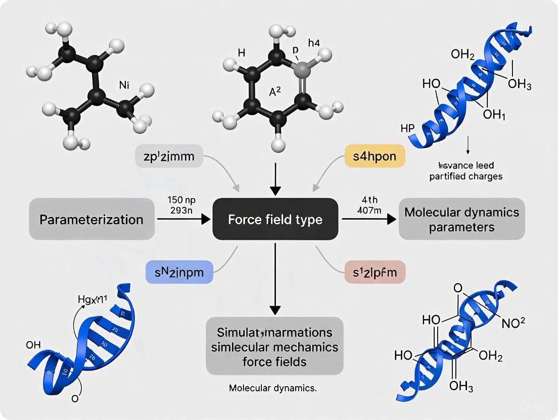
Molecular mechanics (MM) force fields are fast, empirical models that describe the potential energy surfaces of biomolecular systems by treating them as collections of atomic point masses. These models are indispensable for a multitude of tasks in biomolecular simulation and computer-aided drug design, including enumeration of putative bioactive conformations, hit identification via virtual screening, prediction of membrane permeability, simulations of biomolecular dynamics, and estimation of protein-ligand binding free energies via alchemical free energy calculations [1]. Among the various force field classifications, Class I MM force fields represent the most widely used compromise between computational speed and physical accuracy for simulating proteins, lipids, nucleic acids, and other relevant biomolecules [2] [1]. These force fields approximate the quantum mechanical energy surface with a classical mechanical model, thereby decreasing the computational cost of simulations on large systems by orders of magnitude compared to quantum chemical methods [2].

The fundamental trade-off between simplification for speed and physical accuracy forms the core challenge in Class I force field development. While these force fields allow for simulations of biologically relevant systems over meaningful timescales, their simplified functional forms inherently limit their ability to precisely reproduce quantum mechanical potential energy surfaces [3]. This limitation represents a significant source of error in molecular mechanics research, particularly for applications requiring high chemical accuracy, such as binding free energy calculations and conformational analysis. Understanding this trade-off is essential for researchers interpreting simulation results and strategically selecting computational methods for drug development projects.

Mathematical Formulation of Class I Force Fields

Core Functional Form

Class I additive force fields employ a potential energy function that partitions the total energy into bonded (intramolecular) and nonbonded (intermolecular) components. The total potential energy ( U_{\text{MM}} ) of a molecular system with coordinates ( \mathbf{x} ) is defined by the equation:

[ U{\text{MM}}(\mathbf{x};\Phi{\mathtt{FF}}) = \sum{\text{bonds}} \frac{Kr}{2}(r{i,j}-r0)^2 + \sum{\text{angle}} \frac{K\theta}{2}(\theta{i,j,k}-\theta0)^2 ] [

• \sum{\text{torsion}} \sum{n=1}^{n{\text{max}}} K{\phi,n}[1+\cos(n\phi{i,j,k,l}-\phi0)] + \sum{\text{Coulomb}} \frac{1}{4\pi\epsilon0}\frac{qi qj}{r{i,j}} + \sum{\text{van der Waals}} 4\epsilon\left[\left(\frac{\sigma{i,j}}{r{i,j}}\right)^{12}-\left(\frac{\sigma{i,j}}{r{i,j}}\right)^6\right] ]

Where the sets of force field parameters ( \Phi{\mathtt{FF}} = {Kr, K\theta, r0, \theta0, K{\phi,n}, \phi0, q, \sigma, \epsilon}{i} ) are specified for each atom [1]. This separable functional form allows for computational efficiency through the independent calculation of energy components, but introduces physical approximations that limit accuracy.

Component-Specific Mathematical Treatments

The bonded interactions in Class I force fields comprise four distinct types: bond stretching, angle bending, proper dihedrals, and improper dihedrals. Bond stretching and angle bending are modeled as harmonic oscillators, which provides a reasonable approximation near equilibrium geometries but fails to capture anharmonicity effects at higher energies [2]. The torsional energy is represented by a sum of cosine functions with multiplicities n=1,2,3... and amplitudes ( K_{\phi,n} ), providing a periodic potential that captures rotational barriers [2].

Table 1: Mathematical Forms of Bonded Interactions in Class I Force Fields

Interaction Type	Mathematical Form	Parameters Required	Physical Limitations
Bond Stretching	( E{\text{bond}} = Kb(b-b_0)^2 )	Reference bond length ( b0 ), force constant ( Kb )	Harmonic approximation fails for bond dissociation
Angle Bending	( E{\text{angle}} = K\theta(\theta-\theta_0)^2 )	Reference angle ( \theta0 ), force constant ( K\theta )	Cannot capture inversion barriers or anharmonicity
Proper Dihedral	( E{\text{dihedral}} = \sumn K{\phi,n}[1+\cos(n\phi-\deltan)] )	Dihedral amplitude ( K{\phi,n} ), multiplicity ( n ), phase ( \deltan )	Limited to predefined periodicities
Improper Dihedral	( E{\text{improper}} = K\varphi(\varphi-\varphi_0)^2 )	Reference angle ( \varphi0 ), force constant ( K\varphi )	Maintains planar geometry but with simplified potential

The nonbonded interactions consist of electrostatic and van der Waals terms. Electrostatics are handled by Coulomb interactions between fixed point charges ( qi ) and ( qj ) centered on the atoms, known as "partial charges" [2]. This treatment is referred to as "additive" because the charges do not affect each other. For the van der Waals interaction component, a classical Lennard-Jones 6-12 potential is typically used, defined by the radius ( R{\min,ij} ) and the well depth ( \varepsilon{ij} ) [2]. The LJ potential has limitations in its R⁻¹² treatment of atomic repulsion, though this is generally not significant for most biological simulations at room temperature.

Accuracy Limitations and Physical Simplifications

Functional Form Limitations

The mathematical simplifications in Class I force fields introduce systematic errors that limit their physical accuracy. The harmonic approximation for bond and angle terms dominates the local covalent structure around each atom but fails to capture anharmonic effects that become significant at higher energy levels or for systems with floppy degrees of freedom [2]. While this approximation is generally adequate for simulations at room temperature where bond and angle vibrations typically don't reach energy levels where anharmonicity becomes critical, it presents limitations for studying chemical reactions or high-temperature systems.

The treatment of electrostatic interactions using fixed partial atomic charges represents another significant simplification. This approach fails to account for electronic polarization effects, where the charge distribution of a molecule changes in response to its environment [2] [4]. This limitation becomes particularly problematic when simulating heterogeneous environments such as protein-ligand binding interfaces, membrane permeation, or transfer between solvents of different polarities, where the electronic structure of molecules undergoes significant changes [4].

Comparison with Higher-Class Force Fields and Quantum Benchmarks

Class II and III force fields address some limitations of Class I formulations by incorporating anharmonicity and cross-terms. These advanced force fields contain cubic and/or quartic terms in the potential energy for bonds and angles of the form ( E{\text{bond}} = Kb(b - b0)^2 + Kb'(b - b0)^3 + Kb''(b - b0)^4 + \ldots ) [2]. Additionally, they include cross terms that reflect the coupling between adjacent internal coordinates, such as bond-bond cross terms of the form ( E{\text{cross}}(b1,b2) = K{b1,b2}(b1 - b{1,0})(b2 - b_{2,0}) ) [2].

Table 2: Accuracy Comparison Between Force Field Classes

Property	Class I Force Fields	Class II/III Force Fields	Quantum Chemical Reference
Bond Dissociation	Harmonic approximation fails	Anharmonic terms improve dissociation curves	Full potential energy surface
Vibrational Spectra	Limited accuracy for frequencies	Improved through cross terms and anharmonicity	High accuracy with electron correlation
Conformational Energies	Dependent on torsion parametrization	Better transferability through coupling terms	Ab initio or DFT reference
Polarization Effects	None (fixed charges)	Limited (possible with extra terms)	Explicit electron density response
Computational Speed	Fastest	Moderate (2-5x slower than Class I)	3-6 orders of magnitude slower

While anharmonicity and cross terms allow for better reproduction of subtle physical phenomena like vibrational spectra, they have the important disadvantage of multiplying the amount of target data needed for meaningful parameter optimization [2]. This dramatically increases the complexity of the parameter optimization process. The higher target data requirement may not be prohibitive for force fields focused on reproducing the energetics of a limited number of small model compounds in vacuum, where large amounts of uniform and high-quality target data can be obtained through QM calculations. However, such an approach has proven inappropriate for biomolecular force fields used in computational structure-based drug discovery, where nonbonded interactions and precise reproduction of select torsions in the context of a large polymer in the condensed phase are vastly more important than precise reproduction of bond and angle vibrations [2].

Parameterization Methodologies and Their Impact on Accuracy

Traditional Parameterization Approaches

The parametrization of Class I force fields represents a complex optimization problem where parameters are fitted to reproduce both quantum mechanical data and experimental observations. The process involves determining parameters for bonded interactions (bonds, angles, dihedrals) and nonbonded interactions (partial charges, van der Waals parameters) that minimize the difference between force field predictions and reference data [2]. This parameter optimization is challenging due to the coupled nature of the parameters - changing one parameter often affects multiple observable properties.

The assignment of parameters in traditional Class I force fields relies on a scheme termed atom typing, where atoms with similar chemical environments are grouped into types that share identical parameters [3]. This approach reduces the parameter space but introduces approximations, as atoms in similar but distinct chemical environments are treated identically. Takaba et al. showed that on limited chemical spaces and low energy regions, the energy disagreement between legacy force fields and QM is far beyond the chemical accuracy of 1 kcal/mol—the empirical threshold under which qualitative characterization of a many-body system is possible [3]. Even when coupled with a trainable, flexible parametrization engine, the training accuracy still cannot exceed the chemical accuracy, indicating limitations in both the functional form and parametrization steps of MM force fields [3].

Modern Parameterization Tools and Machine Learning Approaches

Recent advances have introduced automated toolkits to facilitate the parameterization process, reducing the burden of developing missing parameters for non-expert users. These include:

• Parmscan and Antechamber for GAFF/GAFF2
• Paramfit for AMBER
• ffTK for CGenFF
• ATB for GROMOS
• LigParGen for OPLS-AA
• Poltype for polarizable FF AMOEBA [4]

Machine learning methods have recently been adopted in force field parameterization for efficiency. Galvelis et al. combined a general force field with several neural network potentials to improve dihedral parameters, demonstrating that small molecules can be parameterized in much shorter time compared to equivalent procedures using density functional theory calculations [4]. Similarly, Martin et al. used machine learning algorithms to rapidly assign partial charges for screening molecules encoded as cyclic undirected graphs with atoms corresponding to vertices and bonds to edges [4].

The Open Force Field Consortium has worked on an approach to automatically recognize chemical moieties and assign parameters via standard chemical substructure queries using the SMIRKS Native Open Force Field format, which identifies specific atoms inside a chemical pattern via an industry-standard SMARTS language and its SMIRKS extensions [4].

Experimental Protocols for Force Field Validation

Standard Validation Methodologies

Validating the performance of Class I force fields requires rigorous comparison against experimental and high-level theoretical data. Standard protocols include:

Conformational Energy Validation: This methodology involves comparing the relative energies of different molecular conformations calculated using the force field against high-level quantum chemical benchmarks. Researchers typically:

• Generate diverse conformers for a set of representative molecules
• Optimize geometries at the quantum mechanical level (e.g., DFT or MP2)
• Calculate single-point energies at higher levels of theory (e.g., CCSD(T)) for accurate relative energies
• Compare with force field predictions for the same conformers
• Compute error metrics such as root mean square error (RMSE) and mean unsigned error (MUE)

Solvation Free Energy Calculations: This protocol assesses how well the force field reproduces the transfer free energies of molecules between gas phase and solution:

• Select a diverse set of small molecules with experimental hydration free energy data
• Perform alchemical free energy simulations (e.g., thermodynamic integration or free energy perturbation)
• Compare calculated solvation free energies with experimental values
• Compute statistical measures of agreement (MUE, R²)

A recent study achieved a mean unsigned error of only 0.37 kcal/mol for the hydration free energy of more than 400 organic solutes using an adjusted bond charge correction model with GAFF2 parameters [4].

Binding Free Energy Validation

For drug discovery applications, validating force field performance for protein-ligand binding free energy predictions is essential:

• Select a diverse set of protein-ligand complexes with experimentally measured binding affinities
• Prepare systems using standard protocols (solvation, ionization, minimization)
• Perform absolute or relative binding free energy calculations using methods such as thermodynamic integration or free energy perturbation
• Compare calculated versus experimental binding affinities
• Compute correlation coefficients and error metrics

The combination of GAFF2 parameters with the new ABCG2 charge model has demonstrated capability in dealing with different dielectric environments, which is important for quantitatively predicting transfer free energies and binding free energies [4].

Table 3: Key Research Reagents and Computational Tools

Tool/Resource	Type	Primary Function	Relevance to Force Field Development
AMBER	Software Suite	Molecular dynamics simulations	Provides implementation and testing platform for force fields
CHARMM	Software Suite	Biomolecular simulation	Alternative force field family with different parametrization philosophy
GAFF/GAFF2	Force Field	General small molecule parameters	Widely used force field for drug-like molecules
CGenFF	Force Field	CHARMM-compatible small molecules	Consistent with CHARMM biomolecular force fields
OPLS3e	Force Field	Expanded drug-like compound parameters	Includes ligand-specific charge assignment
Quantum Chemistry Codes	Software	Ab initio calculations	Generate target data for parametrization
Force Field Toolkits	Utilities	Parameter derivation	Automate parametrization process (e.g., ffTK, Parmscan)
Ligand Test Sets	Datasets	Validation compounds	Provide diverse chemical space for testing

Emerging Solutions and Future Directions

Polarizable Force Fields

Growing effort has been made to address the lack of polarization in additive models by developing polarizable force fields. Classical additive force field models remain problematic when the same set of fixed partial charges is applied to different environments, where the charge distribution is expected to change, such as from gas to aqueous solution, solvent to protein cavity, during cell membrane permeation, and at heterogeneous interfaces [4]. Polarizable force fields address this limitation by allowing charge distributions to respond to their local environment, providing a more physical representation of electrostatic interactions.

Several approaches to polarization have been developed, including:

• Drude oscillator models that introduce virtual particles connected to atoms by springs
• Fluctuating charge models that allow charge transfer between atoms
• Classical induced dipole models that respond to the local electric field

While polarizable force fields offer improved physical accuracy, they come at significantly increased computational cost (typically 3-5 times slower than non-polarizable force fields) and greater parametrization complexity [4].

Machine Learning Force Fields

Machine learning force fields represent a promising direction for bridging the accuracy gap while maintaining computational efficiency. MLFFs use differentiable neural functions parametrized to fit ab initio energies, with forces obtained through automatic differentiation [1] [3]. These models have demonstrated remarkable accuracy, with many recent variants surpassing the chemical accuracy threshold of 1 kcal/mol on limited chemical spaces [3].

The espaloma-0.3 force field exemplifies this approach, using graph neural networks trained on large-scale quantum chemical data (over 1.1 million energy and force calculations) to reproduce quantum chemical energetic properties of chemical domains relevant to drug discovery, including small molecules, peptides, and nucleic acids [1]. This methodology demonstrates significant promise as a path forward for systematically building more accurate force fields that are easily extensible to new chemical domains of interest.

However, the utility of current MLFF models is primarily limited by their speed rather than accuracy. While they are magnitudes faster than QM calculations and scale linearly with system size, they are still hundreds of times slower than traditional MM force fields [3]. For small molecule systems up to 100 atoms, some of the fastest MLFFs still take around 1 millisecond per energy and force evaluation on an A100 GPU, compared to less than 0.005 milliseconds for MM force fields [3].

The Class I force field paradigm represents a carefully balanced compromise between computational efficiency and physical accuracy that has enabled the simulation of biologically relevant systems over meaningful timescales. The simplified functional form—with its harmonic bonds and angles, periodic torsions, and fixed-charge electrostatics—provides the computational speed necessary for studying large biomolecular systems and performing high-throughput virtual screening in drug discovery. However, these very simplifications introduce systematic errors that limit accuracy, particularly for properties sensitive to electronic polarization, anharmonicity, and cross-correlated internal coordinates.

The trade-off between speed and accuracy in Class I force fields manifests across multiple dimensions: in their mathematical formulation, which sacrifices physical fidelity for computational efficiency; in their parametrization strategies, which must balance transferability against chemical specificity; and in their application domains, where they excel at sampling conformational space but struggle with properties requiring quantum mechanical accuracy. Emerging approaches, including polarizable force fields and machine learning potentials, offer promising paths forward but currently face their own trade-offs in complexity, computational cost, and parametrization requirements.

For researchers in computational chemistry and drug discovery, understanding these fundamental trade-offs is essential for selecting appropriate modeling strategies, interpreting simulation results with necessary caution, and developing methodologies that maximize the utility of Class I force fields within their inherent limitations. As force field development continues to evolve, the ideal balance between speed and accuracy may remain context-dependent, varying with the specific scientific question, system characteristics, and available computational resources.

Limitations of Harmonic Oscillators for Bond and Angle Potentials

This technical guide examines the fundamental limitations of harmonic oscillator approximations in modeling bond and angle potentials within molecular mechanics force fields. As force fields remain essential tools for computational structure-based drug discovery (CSBDD) and biomolecular simulations, understanding these inherent constraints is crucial for researchers interpreting simulation results and developing improved models. The harmonic approximation, while computationally efficient, introduces significant errors in predicting vibrational spectra, modeling bond dissociation, and representing potential energy surfaces far from equilibrium geometries. This analysis documents how these limitations propagate into force field parametrization and provides methodological frameworks for assessing their impact on research outcomes, particularly in pharmaceutical applications where accurate conformational dynamics are essential for reliable drug binding predictions.

In molecular mechanics force fields, the potential energy of a system is described using classical mechanical models rather than quantum mechanical calculations, dramatically reducing computational cost for simulations of large biological systems such as proteins in solution [2]. The harmonic oscillator model provides the fundamental mathematical framework for representing bonded interactions—specifically bond stretching and angle bending—in most classical force fields used in computational structure-based drug discovery [2].

The standard class I additive potential energy function decomposes the total energy into bonded and non-bonded terms: E_total = E_bonded + E_nonbonded [5] [2]. The bonded component itself consists of multiple harmonic terms:

Within this framework, bond stretching is typically modeled as a harmonic potential using a Hooke's law formulation: E_bond = k_ij/2 (l_ij - l_0,ij)², where k_ij is the bond force constant, l_ij is the instantaneous bond length, and l_0,ij is the equilibrium bond length between atoms i and j [5]. Similarly, angle bending is represented as a harmonic function of the angle deviation from its equilibrium value [2].

The theoretical basis for these harmonic approximations originates from the Taylor series expansion of the general potential energy curve V(x) around the equilibrium bond distance x_0 [6] [7]:

At the equilibrium position, the first derivative term vanishes, and the potential can be approximated by the quadratic term, yielding the harmonic potential V(x) ≈ (1/2)kx² [6]. While this approximation is reasonably accurate for small displacements near equilibrium, its limitations become significant as molecular vibrations deviate further from the equilibrium geometry.

Fundamental Limitations of the Harmonic Approximation

Inaccurate Representation of Potential Energy Surfaces

The harmonic oscillator model provides only a local approximation of the true potential energy surface, with significant deviations occurring as bond lengths or angles move away from equilibrium positions. As documented in quantum chemistry studies of molecular vibrations, the harmonic approximation fails to capture several critical aspects of real molecular potentials [6] [7]:

• Asymmetric potential energy curves: Real bonds exhibit softer potentials under extension than compression, a fundamental asymmetry that symmetric harmonic potentials cannot represent.
• Finite bond dissociation energies: Harmonic potentials increase without bound as bond lengths increase, unlike real chemical bonds that eventually dissociate.
• Anharmonic vibrational progression: The energy level spacing in real molecules decreases with increasing vibrational quantum number, contrary to the equal spacing predicted by harmonic oscillators.

These limitations become particularly pronounced for systems with soft vibrational modes, low-frequency motions, and in simulations where elevated temperatures populate higher vibrational states.

Inability to Model Bond Dissociation

The harmonic potential's most severe limitation is its fundamental inability to describe bond breaking processes [6] [7]. The quadratic potential V(x) = (1/2)kx² increases without bound as the bond stretch (x) increases, preventing bond dissociation regardless of how much energy is introduced into the system [6]. This restriction has profound implications for force field applications:

• Reactive processes cannot be studied using standard harmonic potentials, eliminating investigations of chemical reactions, enzyme mechanisms, or bond rupture under mechanical stress.
• High-temperature simulations become unreliable as thermal energy approaches significant fractions of the bond dissociation energy.
• Stress-strain relationships in materials modeling deviate significantly from experimental measurements at high deformation.

For these applications, more sophisticated potentials such as the Morse potential must be employed to accurately represent the bond dissociation limit [7].

Spectral Predictions and Overtone Transitions

The quantum harmonic oscillator model predicts equally spaced energy levels according to E_v = (v + 1/2)ν_e, where v is the vibrational quantum number [6]. This equal spacing leads to the prediction of only a single fundamental vibrational transition frequency, with no allowed overtones [6] [7]. This contradicts experimental spectroscopic observations:

• Multiple overtone transitions are routinely observed in experimental vibrational spectra of molecules [6].
• Vibrational energy levels in real molecules become progressively closer with increasing vibrational quantum number, following the anharmonic expression: E_v = (v + 1/2)ν_e - (v + 1/2)²ν_ex_e + (v + 1/2)³ν_ey_e + ... where x_e and y_e are anharmonicity constants [6] [7].
• Infrared absorption intensities for overtone transitions cannot be predicted within the harmonic approximation.

These limitations reduce the utility of harmonic force fields for predicting or matching experimental vibrational spectra, necessitating empirical scaling factors for frequency calculations.

Table 1: Quantitative Comparison of Harmonic and Anharmonic Oscillator Properties

Property	Harmonic Oscillator	Real Molecular Vibrations
Potential Energy Function	V(x) = (1/2)kx²	V(x) = (1/2)kx² + (1/6)γx³ + ... [6]
Energy Level Spacing	Equal: ΔE = constant	Decreasing with v [6] [7]
Bond Dissociation	Not possible	Finite dissociation energy D_e [6]
Overtone Transitions	Forbidden	Observed experimentally [6]
Vibrational Frequency	ν = (1/2π)√(k/μ)	Modified by anharmonicity [6]

Consequences for Force Field Parametrization and Performance

Parametrization Constraints and Compromises

The use of harmonic potentials for bond and angle terms imposes significant constraints on force field parametrization strategies, often forcing compromises between different physical properties [2]. Parameter optimization becomes particularly challenging because:

• Limited transferability: Parameters optimized for small displacements near equilibrium may perform poorly for distorted geometries encountered in flexible molecules or strained systems.
• Compensating errors: Inaccuracies in harmonic bond terms may be partially compensated by adjustments in other force field parameters, particularly in class I additive force fields where the simple functional forms lack the flexibility to accurately represent all aspects of the potential energy surface [2].
• Temperature dependence: Harmonic force constants lack intrinsic temperature dependence, though real vibrational frequencies exhibit temperature effects due to anharmonicity.

As noted in molecular mechanics research, "the biomolecular force field community has until recently refrained from introducing anharmonicity and cross terms, recognizing that there was still plenty of room for improvements within the framework of the class I potential energy function" [2]. This reflects the practical compromise between physical accuracy and parametrization feasibility that harmonic potentials represent.

Impact on Conformational Sampling and Dynamics

The harmonic approximation significantly affects molecular dynamics simulations and conformational sampling in ways that can influence research conclusions:

• Restricted phase space sampling: The harmonic potential excessively constrains bond lengths and angles, potentially inhibiting access to some conformational states that would be accessible with more flexible potentials.
• Inaccurate energy distributions: The harmonic approximation misrepresents the relative energies of different molecular geometries, particularly for distorted structures far from equilibrium.
• Vibrational energy redistribution: Coupling between different vibrational modes, represented by cross terms in more sophisticated force fields, is absent in standard harmonic potentials [2].

These limitations become particularly important in biomolecular simulations where subtle energy differences between conformational states can determine binding affinities, folding pathways, and allosteric mechanisms relevant to drug design.

Table 2: Advanced Potential Functions Beyond Harmonic Approximation

Potential Type	Functional Form	Advantages	Computational Cost
Morse Potential	E_bond = D_e[1 - e^{-a(r-r_0)}]²	Describes bond dissociation [5]	High
Quartic Bond Potential	E_bond = K_b(b-b_0)² + K_b'(b-b_0)³ + K_b″(b-b_0)⁴	Better PES reproduction [2]	Moderate
Cross Terms	E_cross = K_b1,b2(b1-b1,0)(b2-b2,0)	Coupling between internal coordinates [2]	Moderate
Class II/III Force Fields	Includes anharmonic + cross terms	Accurate vibrational spectra [2]	High

Methodological Framework for Assessment

Experimental Protocols for Validation

Researchers should employ the following methodological approaches to assess the impact of harmonic potential limitations in their specific applications:

Vibrational Frequency Analysis Protocol:

• Perform geometry optimization of the molecular system
• Calculate vibrational frequencies using harmonic force field
• Compare predicted frequencies with experimental infrared and Raman spectra
• Identify systematic deviations, particularly in overtone regions
• Calculate empirical scaling factors to correct systematic errors

Conformational Energy Benchmarking:

• Generate diverse molecular conformations with varying bond lengths and angles
• Calculate relative energies using both the force field and high-level quantum mechanical methods
• Quantify errors for distorted geometries far from equilibrium
• Analyze correlation between distortion magnitude and energy error

Thermodynamic Property Validation:

• Run molecular dynamics simulations at multiple temperatures
• Calculate thermodynamic properties (heat capacities, free energies)
• Compare with experimental data where available
• Identify temperature-dependent deviations potentially attributable to harmonic limitations

Computational Workflow for Force Field Evaluation

The diagram below illustrates a systematic workflow for evaluating harmonic potential limitations in molecular mechanics force fields:

Advanced Modeling Approaches

Beyond Harmonic Potentials: Anharmonic Formulations

To address the limitations of harmonic potentials, several more sophisticated approaches have been developed:

Morse Potentials: The Morse potential provides a more realistic representation of bond stretching that incorporates bond dissociation: E_bond = D_e[1 - e^{-a(r-r_0)}]², where D_e is the dissociation energy and a controls the potential width [5] [7]. While computationally more expensive, this potential correctly describes bond breaking and the decreasing spacing of vibrational levels with increasing energy.

Class II and III Force Fields: These advanced force fields incorporate cubic and quartic terms in the potential energy for bonds and angles: E_bond = K_b(b - b_0)² + K_b'(b - b_0)³ + K_b″(b - b_0)⁴ + ... [2]. Additionally, they include cross terms that reflect coupling between adjacent internal coordinates, such as bond-bond terms of the form E_cross(b1,b2) = K_b1,b2(b1 - b1,0)(b2 - b2,0) [2].

Urey-Bradley Terms: Some force fields include Urey-Bradley terms, which consist of harmonic potentials between atoms A and C of an A-B-C angle, effectively creating a coupling between angle bending and nonbonded interactions between the terminal atoms [2].

The Scientist's Toolkit: Research Reagent Solutions

Table 3: Essential Computational Tools for Advanced Force Field Development

Tool/Category	Specific Examples	Function/Purpose
Quantum Chemistry Software	Gaussian, ORCA, Q-Chem	Generate target data for parametrization [2]
Force Field Parametrization Platforms	CGenFF, MATCH, LigParGen	Develop transferable parameters [5]
Molecular Dynamics Engines	GROMACS, NAMD, OpenMM, AMBER	Perform simulations with anharmonic potentials [5] [2]
Spectral Analysis Tools	Mol vibrational, SPECDIS	Compare calculated and experimental spectra [6]
Force Field Databases	OpenKIM, TraPPE, MolMod	Access validated parameters [5]
Polarizable Force Fields	AMOEBA, CHARMM Drude	Model electronic polarization effects [2]

The harmonic oscillator model for bond and angle potentials provides computational efficiency at the cost of significant physical approximations that limit accuracy in molecular simulations. While adequate for many applications involving biomolecules near their equilibrium geometries, these limitations become critical when studying processes involving large-amplitude motions, bond dissociation, spectroscopic properties, or highly strained molecular systems.

Future directions in force field development aim to address these limitations through several promising approaches:

• Polarizable force fields that go beyond fixed partial charges to model electronic polarization effects [2].
• Machine learning potentials that can capture complex aspects of potential energy surfaces without explicit functional forms.
• Multi-scale modeling approaches that apply more accurate potentials where needed while maintaining efficiency elsewhere.
• Systematic parameter optimization using expanded target data sets that include spectroscopic properties and quantum mechanical calculations of distorted geometries [2].

For researchers in force field development and computational drug discovery, acknowledging these limitations is essential for appropriate application and interpretation of molecular simulations. Continued refinement of potential energy functions remains crucial for improving the predictive power of computational models in structural biology and drug design.

The Challenge of Torsional Parameterization and Conformational Energetics

In molecular mechanics (MM) force fields, the accurate representation of a molecule's potential energy surface (PES) is fundamental to the reliability of molecular dynamics simulations in drug discovery. The mathematical model decomposes this energy into bonded (bonds, angles, torsions) and non-bonded (electrostatics, van der Waals) terms [8]. Among these, torsional parameters present a singular challenge. They must capture the complex stereoelectronic and steric effects that dictate rotational energy profiles, which are crucial for predicting conformational distributions and, consequently, properties like protein-ligand binding affinity [9] [8].

The core of the challenge lies in the inherent transferability problem. While other valence parameters are largely determined by local chemical environments, torsional potentials are exceptionally sensitive to non-local effects and the specific chemical context [9]. This document, framed within a broader thesis on common error sources in force field research, elucidates why torsional parameterization remains a critical bottleneck and details the modern, data-driven strategies being developed to overcome it.

The Critical Role of Torsional Parameters in Drug Discovery

The accuracy of torsional parameters directly impacts the predictive power of simulations in computational drug discovery. An incorrectly parameterized torsion can lead to an inaccurate representation of a ligand's low-energy conformations, which can propagate errors into critical calculations.

• Conformational Populations and Binding Affinity: The conformational preferences of a drug-like molecule influence its binding mode and affinity. Force fields that poorly reproduce quantum mechanical (QM) torsional profiles will fail to predict the correct Boltzmann-weighted ensemble of conformers, leading to errors in alchemical binding free energy calculations [9].
• Real-World Impact: A study on a congeneric series of TYK2 kinase inhibitors demonstrated that refining torsional parameters with bespoke fitting reduced the mean unsigned error (MUE) in binding free energy predictions from 0.56 kcal/mol to 0.42 kcal/mol and improved the R² correlation from 0.72 to 0.93. This level of improvement can significantly enhance the reliability of computational guides for lead optimization [9].

Comparative Analysis of Modern Force Field Parameterization Strategies

The field is moving beyond traditional "look-up table" approaches. The table below summarizes and compares the core methodologies of three modern parameterization strategies, highlighting how they address the torsion challenge.

Table 1: Comparison of Modern Force Field Parametrization Approaches

Feature	Traditional Look-up Table (e.g., OPLS3e)	SMIRKS-Based Perception (e.g., OpenFF)	Data-Driven & ML-Based (e.g., ByteFF, Espaloma)
Core Philosophy	Pre-defined library of torsion parameters for specific atom type combinations.	Assigns parameters via chemical substructure queries (SMARTS patterns).	Uses machine learning models trained on QM data to predict parameters end-to-end.
Handling of Torsions	Large number of specific torsion types (e.g., 146,669 in OPLS3e); bespoke fitting tools (e.g., FFBuilder) for new chemistry [9] [8].	Compact, hierarchical parameters; bespoke fitting (BespokeFit) for problematic torsions [9].	Graph Neural Network (GNN) predicts all parameters simultaneously, including torsions, for any given molecule [10] [8].
Chemical Coverage	Limited by the pre-determined list; requires continuous expansion [8].	Good transferability via SMIRKS; extension is straightforward [9].	Designed for "expansive chemical space coverage" by learning from a massive, diverse dataset [11].
Key Advantage	Well-established, high accuracy for covered chemistry.	Reduces parameter redundancy; systematic and automated bespoke refinement.	High transferability and scalability; avoids discrete chemical perception limitations [8].
Reported Performance	High accuracy but challenges with transferability.	Bespoke fitting reduced torsion RMSE from 1.1 kcal/mol to 0.4 kcal/mol on a test set [9].	State-of-the-art performance on relaxed geometries, torsional profiles, and conformational energies [10].

Experimental Protocols for Addressing the Torsion Challenge

The strategies in Table 1 rely on sophisticated experimental and computational protocols to generate high-quality reference data. The following workflows are central to modern force field development.

Workflow for Data-Driven Force Field Development (e.g., ByteFF)

This protocol involves creating a large-scale QM dataset and training a machine-learning model to predict parameters [8].

Key Protocol Steps:

• Molecular Dataset Curation: A diverse set of drug-like molecules is selected from databases like ChEMBL and ZINC20 based on criteria including aromatic rings, polar surface area (PSA), and quantitative estimate of drug-likeness (QED) [8].
• Fragmentation: Molecules are cleaved into smaller fragments (<70 atoms) using a graph-expansion algorithm. This preserves local chemical environments and makes QM calculations tractable [8].
• Protonation State Expansion: Fragments are expanded to various protonation states within a physiologically relevant pKa range (0.0–14.0) to ensure comprehensive coverage [8].
• Quantum Mechanical Calculations: A massive QM dataset is generated at the B3LYP-D3(BJ)/DZVP level of theory, balancing accuracy and computational cost. This produces:
  • Optimization Dataset: 2.4 million optimized molecular fragment geometries with analytical Hessian matrices.
  • Torsion Dataset: 3.2 million torsion scans, which provide the rotational energy profiles used to fit torsion parameters [10] [8] [11].
• Machine Learning Training: An edge-augmented, symmetry-preserving Graph Neural Network (GNN) is trained on this dataset. A carefully optimized training strategy, including a differentiable partial Hessian loss, is used to simultaneously predict all bonded and non-bonded MM parameters for a given molecule [8].

Workflow for Automated Bespoke Torsion Parameterization (e.g., BespokeFit)

This protocol is designed to refine torsion parameters for specific molecules of interest, often within a project context [9].

Key Protocol Steps:

• Fragmentation: The target molecule is automatically fragmented around each rotatable bond of interest. Tools like the OpenFF Fragmenter are used to generate smaller, representative fragments that closely mimic the torsional potential of the central bond in the parent molecule [9] [12]. This significantly reduces the computational cost of subsequent QM calculations.
• SMIRKS Generation: A unique SMIRKS pattern is generated to describe the chemical environment of each torsion being parameterized, ensuring compatibility with the SMIRNOFF force field format [9].
• Reference Data Generation: Torsion scans are performed for each fragment. Modern implementations offer a choice of methods:
  • Machine Learning Potentials: Using ANI-2X, a deep learning potential, provides accuracy close to its reference DFT (ωB97X/6-31G(d)) at a fraction of the cost (e.g., minutes per scan) [12].
  • Semi-Empirical Methods: Using methods like xTB can offer even greater speed (over 30x faster than ANI-2X in some cases) for rapid profiling [12].
  • Traditional QM: DFT calculations remain the gold standard for generating reference data [9].
• Parameter Optimization: The tool ForceBalance is used to optimize the torsion force constants (kϕ) and phase offsets (ϕ0) to minimize the difference between the MM and reference QM torsion potential energy surfaces [9] [12].

The Scientist's Toolkit: Essential Research Reagents and Software

Table 2: Key Software and Resources for Advanced Force Field Parameterization

Tool Name	Type	Primary Function in Parameterization
BespokeFit [9]	Software Package	Automates the creation of bespoke torsion parameters for individual molecules within the OpenFF ecosystem.
QCSubmit [9]	Software Tool	Simplifies the creation, submission, and retrieval of large quantum chemical calculation datasets to QCArchive.
ForceBalance [12]	Optimization Tool	Systematically optimizes force field parameters against reference QM and experimental data.
OpenFF Fragmenter [9]	Fragmentation Tool	Performs torsion-preserving fragmentation to generate smaller molecules for efficient QM torsion scans.
ANI-2X [12]	Machine Learning Potential	Provides fast, accurate torsion energy profiles as a surrogate for more expensive DFT calculations.
xTB [12]	Semi-Empirical QM Method	Offers a very fast method for geometry optimization and torsion scanning, useful for high-throughput workflows.
TorsionDrive [12]	Algorithm	Implements wavefront propagation to efficiently and reliably perform torsion scans, ensuring smooth potential energy surfaces.
Graph Neural Networks [8]	Machine Learning Model	Used in data-driven FFs (e.g., ByteFF, Espaloma) to predict all MM parameters directly from molecular graph.
B3LYP-D3(BJ)/DZVP [8]	QM Method & Basis Set	A commonly used level of theory for generating benchmark-quality reference data for force field training.

The challenge of torsional parameterization is a central source of error in molecular mechanics, directly impacting the predictive accuracy of simulations in drug discovery. The field is actively transitioning from reliance on extensive parameter libraries to more intelligent, automated, and data-driven paradigms. Strategies range from automated bespoke fitting for specific project molecules to the development of next-generation, ML-native force fields like ByteFF that learn parameters from massive quantum chemical datasets. These approaches, leveraging advanced software tools and machine learning, are poised to provide the accuracy, transferability, and expansive chemical coverage required for the next generation of computational drug discovery.

Fixed Charge Models and the Neglect of Electronic Polarization

Molecular Mechanics (MM) force fields are indispensable tools in computational chemistry and structure-based drug discovery, enabling the simulation of proteins and other biological macromolecules at a feasible computational cost [2]. For decades, the predominant approach has employed fixed charge models, where electrostatic interactions are represented by point charges permanently assigned to atomic centers [13] [14]. These "additive" force fields, classified as Class I, sum bonded and nonbonded terms to calculate a system's total energy, with electrostatics governed by Coulomb's law between static partial charges [13]. This simplification has facilitated numerous scientific advances but introduces a fundamental physical omission: the neglect of electronic polarization. Polarization, the redistribution of electron density in response to the local electric field, is a critical phenomenon in molecular interactions [13]. This guide examines the theoretical shortcomings, practical consequences, and emerging solutions related to this significant approximation within the broader context of error sources in molecular mechanics force fields.

Theoretical Foundation of Molecular Mechanics Force Fields

The Class I Potential Energy Function

The functional form of a Class I force field, underlying popular frameworks like AMBER, CHARMM, and OPLS, decomposes the total energy into bonded and nonbonded components [13] [2]. The bonded terms maintain molecular structure, while the nonbonded terms describe intermolecular interactions and intra-molecular interactions between atoms separated by three or more bonds.

The total energy is given by: Etotal = Ebonded + E_nonbonded

The bonded energy is calculated as:

This includes harmonic potentials for bond stretching (b) and angle bending (θ), an improper dihedral term (φ) to maintain chirality and planarity, and a periodic potential for proper dihedral angles (ϕ) [2].

The nonbonded energy is calculated as:

This comprises Coulomb's law for electrostatic interactions between point charges q_i and q_j, and a Lennard-Jones potential describing van der Waals interactions through a repulsive (R^-12) and an attractive (R^-6) term [13] [2].

The Physical Origin of Polarization

From a quantum mechanical perspective, intermolecular interaction energy comprises several components: electrostatic, induction (polarization), dispersion, and exchange repulsion [13]. Polarization energy results from a molecule's electron cloud being distorted by the electric field of its neighbors. This includes the induction energy, where a molecule's permanent multipoles induce moments in another, and dispersion energy, stemming from correlations between instantaneously induced multipoles [13].

Polarization is inherently non-additive. The interaction between two molecules is altered when a third molecule is present, as it polarizes both participants, changing their charge distributions [13]. Fixed charge models, by design, cannot capture this effect. Their parameters are "effective" and tuned to approximate the average polarization in a specific environment (like liquid water), fundamentally limiting their transferability across different dielectric environments [13] [14].

Limitations and Consequences of Neglecting Polarization

Theoretical Shortcomings

The fixed charge approximation suffers from several fundamental physical shortcomings:

• Inability to Model Environmental Response: A molecule's electronic structure differs in a protein binding site, a lipid membrane, or aqueous solution. Fixed charge models use a single, static charge set for all environments, failing to capture this critical response [14].
• Lack of Non-additivity: As polarization is a many-body effect, the presence of a third molecule alters the pairwise interaction between two others. Fixed charge models, being purely additive, cannot reproduce this behavior [13].
• Poor Representation of Anisotropic Charge Distributions: Atom-centered point charges produce a spherical electrostatic potential around an atom. This fails to capture anisotropic features such as sigma-holes (responsible for halogen bonding), electron lone pairs, and π-orbitals, which require higher-order multipoles or off-center charges for accurate description [14].

Practical Implications in Biomolecular Simulations

These theoretical shortcomings manifest as quantifiable errors in simulating biological processes critical to drug discovery.

Table 1: Common Errors from Neglecting Polarization

System/Process	Error Manifestation	Physical Reason
Ion Channels & Transporters	Inaccurate ion selectivity, binding affinity, and free energy profiles [15] [14].	Ions, especially divalent cations (Mg²⁺, Ca²⁺), create strong, local electric fields that dramatically polarize coordinating groups, an effect absent in fixed charge models.
Ligand Binding	Errors in binding energies and poses, particularly for charged ligands or binding sites with strong electrostatic fields.	The ligand's charge distribution in solution differs from that in the protein's binding site. Fixed charges cannot adapt, leading to misrepresentation of the interaction energy.
Membrane-Protein Systems	Poor description of protein-lipid interactions and ion permeation.	The heterogeneous dielectric environment (low-dielectric membrane, high-dielectric water, and protein) creates strong, varying electric fields that induce polarization.

A prominent example is the solvation and ligand exchange of the Mg²⁺ ion. Quantum chemistry calculations show that the polarizability of water molecules is significantly suppressed in the first solvation shell of Mg²⁺ due to the ion's intense electric field and Fermi repulsion with the water's electrons [15]. Fixed-charge models, and even early polarizable models with constant polarizabilities, fail to quantitatively describe the energetics of Mg²⁺-water clusters and dramatically underestimate the water residence time in the ion's solvation shell (e.g., predicting ~10⁻⁹ s versus an experimental value of ~10⁻⁶ s to 10⁻⁵ s) [15]. This error arises because an over-polarizable water model makes the transition state for the ligand exchange reaction too stable, accelerating the kinetics unrealistically [15].

Experimental and Computational Methodologies

Protocols for Quantifying Polarization Effects

Researchers use specific computational protocols to diagnose errors stemming from the neglect of polarization and to parameterize improved models.

Energy Decomposition Analysis (EDA): This quantum mechanical method decomplicates the interaction energy between molecules (e.g., a drug and its protein target) into physically meaningful components: electrostatic, induction (polarization), dispersion, and exchange-repulsion [13]. By comparing the induction energy from EDA to the interaction energy in a fixed-charge force field, the magnitude of the missing polarization component can be quantified.

Supermolecular Approach: The interaction energy is calculated as the difference between the energy of the complex (E_AB) and the energies of the isolated monomers (E_A and E_B): E_int = E_AB - E_A - E_B [13]. This can be performed at a high quantum mechanical (QM) level of theory and compared against force field results to identify systematic deviations in specific molecular arrangements.

Parameterization of Variable Polarizability Models: As demonstrated in the Mg²⁺ case, a variable polarizability model can be derived as follows [15]:

• Cluster Calculations: Perform QM calculations (e.g., MP2) on small clusters, such as a Mg²⁺ ion paired with one or more water molecules.
• Property Fitting: Extract the dipole moment of the water molecule as a function of its distance from the Mg²⁺ ion.
• Model Derivation: Derive an explicit function that describes the water's polarizability based on the distance to the ion. This function is designed to reproduce the QM-derived dipole moments.
• Validation: The new model is tested by simulating properties like cluster energies, solvation free energy, and ligand exchange kinetics, ensuring consistency across different system sizes and conditions [15].

The Scientist's Toolkit: Research Reagent Solutions

Table 2: Essential Computational Tools for Polarization Research

Tool/Reagent	Function/Brief Explanation
Polarizable Force Fields	Empirical models that explicitly include polarization. Key implementations include AMOEBA (induced dipole), CHARMM DRUDE (Drude oscillator), and FLUC (fluctuating charge) [15] [14].
Quantum Chemistry Software	Used to compute reference data (e.g., interaction energies, dipole moments, polarizabilities) for force field development and validation. Examples: Gaussian, GAMESS, Psi4.
Thole Damping Scheme	A critical computational remedy to prevent "polarization catastrophe"—the unrealistic divergence of induced dipoles at short distances—by smearing dipole densities [15] [14].
Molecular Dynamics Engines	Software that performs the actual simulations. Modern packages like OpenMM, AMBER, NAMD, and GROMACS now support polarizable force fields [15] [14].
Multipole Electrostatics	A more advanced representation of the permanent charge distribution using atomic dipoles and quadrupoles, which improves the description of anisotropic effects before polarization is even applied [14].

Diagram: A taxonomy of molecular force fields, highlighting the fundamental division between additive fixed-charge models and polarizable approaches, along with their key characteristics.

Emerging Solutions: Polarizable Force Fields

To overcome the limitations of fixed charge models, significant effort is devoted to developing polarizable force fields. These models explicitly treat the response of the electron cloud to its environment, offering greater transferability and physical fidelity [15] [14]. The three primary classical approaches are:

• Induced Dipole Model: Each atom is assigned a polarizability (α), allowing it to develop an induced dipole (μ_ind) in response to the total electric field (E), such that μ_ind = αE [14]. The total electric field includes contributions from other permanent and induced moments, requiring a self-consistent field (SCF) calculation to converge the dipoles. The AMOEBA force field is a prominent example using this approach [15] [14].
• Drude Oscillator Model: Also known as the "charge-on-spring" model, this approach attaches a fictitious, massless Drude particle (carrying a negative charge) to an atom via a harmonic spring. The displacement of this particle in an electric field creates an induced dipole moment [14]. The CHARMM DRUDE force field is a leading implementation of this model.
• Fluctuating Charge (FQ) Model: Also based on electronegativity equalization, this model allows atomic partial charges to fluctuate in response to the molecular environment to equalize the chemical potential at each atomic site [14].

Table 3: Comparison of Polarizable Force Field Methodologies

Feature	Induced Dipole (AMOEBA)	Drude Oscillator	Fluctuating Charge (FQ)
Physical Basis	Polarizability tensor	Displaced charge in harmonic well	Electronegativity equalization
Computational Cost	Moderate (requires SCF)	Moderate (requires SCF or extended Lagrangian)	Lower
Key Advantage	Naturally captures anisotropic polarization	Intuitive, avoids polarization catastrophe	Describes charge transfer
Key Challenge	Requires Thole damping to prevent "polarization catastrophe" [15]	Parameterizing spring constants and charges	Poorly describes out-of-plane polarization of ions

Recent advancements, such as the variable polarizability model implemented for AMOEBA, address the fact that molecular polarizability is not a constant but depends on the intermolecular distance and the strength of the electric field [15]. This model successfully reproduced the energetics of Mg²⁺-water clusters and the slow kinetics of the water exchange reaction, a feat not achievable with fixed-charge or constant-polarizability models [15].

The use of fixed charge models, while computationally efficient, introduces a significant source of error in molecular mechanics simulations by neglecting the fundamental physical process of electronic polarization. This limitation manifests in inaccurate descriptions of ion chemistry, ligand-binding energetics, and processes occurring in heterogeneous environments like membranes. While these models are "effective" for the conditions they were parameterized for, their lack of transferability hinders predictive accuracy in complex biological contexts. The ongoing development and refinement of polarizable force fields, which explicitly model the environmental response of electron clouds, represent a crucial direction for the future of biomolecular simulation. These advanced force fields promise a more physically grounded and universally applicable framework, ultimately leading to more reliable insights in basic research and more robust predictions in structure-based drug design.

Molecular mechanics (MM) force fields are indispensable tools for biomolecular simulation and computer-aided drug design, enabling researchers to study protein dynamics, predict ligand binding, and explore biological mechanisms at the atomic level. These empirical models approximate the potential energy surface of molecular systems through simple functional forms that balance computational efficiency with physical meaningfulness [16] [2]. Class I additive force fields, the most widely used type for biomolecular simulations, decompose the total potential energy into bonded terms (bonds, angles, torsions) and non-bonded terms (electrostatics and van der Waals interactions) [2]. The blessing and curse of these force fields lies in their simple functional forms: they afford linear runtime complexity and can be aggressively optimized on modern hardware, simulating hundreds of nanoseconds per day for biomolecular drug targets while achieving useful accuracy for tasks like predicting protein-ligand binding free energies [16] [17]. However, this computational efficiency comes at a significant cost—limited expressiveness that makes accurately fitting quantum mechanical energies and forces, particularly in high-energy regions, fundamentally challenging [17].

The core architectural flaw creating transferability issues in traditional MM force fields is the atom-typing scheme—a human-derived, labor-intensive classification system where atoms are forced into discrete categories representing distinct chemical environments [16] [17]. This approach creates an intractable mixed discrete-continuous optimization problem that imposes strong practical limits on accuracy [16]. As chemical space expands, particularly in drug discovery where novel molecular entities frequently push boundaries, this fundamental limitation becomes increasingly problematic, compromising the reliability of simulations and necessitating alternative approaches.

The Combinatorial Explosion Problem: Mathematical Formulation and Consequences

The Atom-Type Paradigm and Its Limitations

In traditional force field development, expert knowledge of physical organic chemistry builds atom-typing rules that classify atoms into discrete categories, enabling molecular mechanics parameters to be subsequently assigned from a table of relevant atomic, bond, angle, and torsion parameters [16]. This approach creates a hierarchical dependency: the assignment of atom types determines available bond parameters, which in turn determine angle parameters, and finally torsion parameters. The accuracy of traditional force fields is therefore limited by the resolution of chemical perception, which itself is limited by the number of distinct atom types [16].

The mathematical reality is that attempting to improve accuracy by increasing the number of atom types results in a combinatorial explosion of bond, angle, and torsion parameters. If a force field contains A atom types, the potential number of:

• Bond parameters scales with A²
• Angle parameters scales with A³
• Torsion parameters scales with A⁴

This exponential relationship imposes strong practical limits on chemical resolution [16]. For example, a force field with 100 atom types could theoretically require up to 100,000,000 torsion parameters—an impossibly large parameter space to systematically optimize. In practice, this means force field developers must make difficult compromises, grouping chemically distinct environments into broad atom types and sacrificing accuracy for feasibility.

Practical Consequences for Biomolecular Simulation

The combinatorial explosion problem manifests in several critical limitations for practical research applications:

• Limited Chemical Coverage: Traditional force fields struggle with the rapid expansion of synthetically accessible chemical space, particularly in drug discovery where novel molecular entities frequently push boundaries [10]. The look-up table approach faces significant challenges in providing adequate parameters for unusual functional groups or complex heterocycles commonly found in pharmaceutical compounds.

• Incompatible Force Field Combinations: To tame the explosion of atom type complexity, biomolecular force field efforts frequently take a divide-and-conquer approach, building separate models for proteins, small molecules, nucleic acids, lipids, and other biomolecules independently [16]. The recent AmberTools 23 release recommends combining independently developed force fields for different chemical domains, representing more than 100 person-years of collective effort [16]. However, using these separate force fields together introduces significant caveats when multiple classes of biomolecules interact, risking poor accuracy and creating frustration when molecules of different classes must be covalently bonded [16].

• Parametrization Inconsistencies: There are often overlaps in the chemical space that each specialized force field is designed to model, with no guarantee that parameters in these overlapping regions are identical and remain compatible [16]. This lack of self-consistency introduces errors in heterogeneous systems, particularly at interfaces between different molecular classes.

• Extensibility Challenges: Extension or expansion to new classes of biomolecules or chemical spaces becomes a time-consuming ordeal, as combining force fields results in a large combinatorial space of possible force field parameters where quality depends heavily on user choices [16].

Table 1: Quantitative Manifestations of the Combinatorial Explosion Problem

Aspect	Traditional Approach	Consequence	Impact on Research
Chemical Coverage	Limited by fixed atom types	Inadequate parameters for novel compounds	Compromised drug discovery simulations
Parameter Space	Grows as A⁴ for torsions	Practical limit on atom type resolution	Systematic error in complex molecules
System Compatibility	Separate protein, small molecule, nucleic acid FFs	Inconsistent parameters at interfaces	Reduced accuracy in protein-ligand systems
Extension Effort	Manual atom type creation	Labor-intensive for new chemical domains	Slow adaptation to new research areas

Beyond Atom Types: Machine Learning Solutions

Graph Neural Networks for Continuous Chemical Perception

Machine learning approaches, particularly graph neural networks (GNNs), represent a paradigm shift in addressing the combinatorial explosion problem. The Espaloma (extensible surrogate potential optimized by message passing) framework replaces rule-based discrete atom-typing schemes with continuous atomic representations generated by graph neural networks that operate on chemical graphs [16]. These atom representations are coupled with symmetry-preserving pooling layers and feed-forward neural networks to enable fully end-to-end differentiable construction of MM force fields [16].

In this approach, the neural network parameters are optimized directly using standard machine learning frameworks to fit quantum chemical and/or experimental data. The expressiveness of Espaloma's continuous atomic representations eliminates the need to combine force fields developed for different chemical domains, enabling self-consistent parametrization of any system of molecules with elemental coverage in its training set [16]. This represents a fundamental architectural improvement over traditional atom-typing schemes.

Hybrid Physical-Machine Learning Models

Another innovative approach involves hybrid models that integrate physics-based molecular mechanics covalent terms with machine learning corrections. ResFF (Residual Learning Force Field) employs deep residual learning to integrate physics-based learnable molecular mechanics covalent terms with residual corrections from a lightweight equivariant neural network [18]. Through a three-stage joint optimization, the two components are trained in a complementary manner to achieve optimal performance [18].

This hybrid approach maintains the physical interpretability of traditional force fields while leveraging machine learning to correct systematic errors, particularly in challenging regions of the potential energy surface such as torsion profiles and non-bonded interactions [18].

Diagram 1: Traditional vs. machine learning approaches to force field parametrization, highlighting how ML methods bypass the combinatorial explosion problem through continuous representations.

Quantitative Performance Comparison

Accuracy Benchmarks Across Chemical Spaces

Modern machine learning force fields demonstrate significant improvements in accuracy across diverse chemical domains compared to traditional approaches. Espaloma-0.3, trained in a single GPU-day on a diverse quantum chemical dataset of over 1.1 million energy and force calculations for 17,000 unique molecular species, reproduces quantum chemical energetic properties of small molecules, peptides, and nucleic acids more accurately than established MM force fields widely used in biomolecular simulation and drug design [16]. The model maintains quantum chemical energy-minimized geometries of small molecules and preserves condensed phase properties of peptides and folded proteins, enabling stable simulations that lead to highly accurate predictions of binding free energies [16].

Similarly, ByteFF—an Amber-compatible force field for drug-like molecules developed using a data-driven approach—demonstrates state-of-the-art performance across various benchmark datasets, excelling in predicting relaxed geometries, torsional energy profiles, and conformational energies and forces [10]. This performance stems from training on an expansive and highly diverse molecular dataset including 2.4 million optimized molecular fragment geometries with analytical Hessian matrices, along with 3.2 million torsion profiles [10].

Table 2: Performance Comparison of Traditional vs. Machine Learning Force Fields

Metric	Traditional MM	ML-Enhanced (Espaloma-0.3)	Improvement
Training Data	~100 person-years [16]	1.1M QC calculations [16]	Quantitative scalability
Parametrization Time	Months to years	Single GPU-day [16]	~100x acceleration
Chemical Coverage	Separate biomolecular classes [16]	Unified small molecules, peptides, nucleic acids [16]	Self-consistent parametrization
Binding Free Energy Prediction	Useful accuracy [17]	Highly accurate [16]	Qualitative improvement
Extensibility	Manual effort for new domains	Automatic via retraining [16]	Fundamental architectural advantage

Limitations and Error Propagation in Machine Learning Force Fields

Despite their promising performance, machine learning force fields face their own challenges. While MLIPs often achieve small average errors in energies and atomic forces (as low as 1 meV atom⁻¹ and 0.05 eV Å⁻¹ respectively), these low averaged errors do not guarantee accurate reproduction of physical phenomena in atomistic simulations [19]. MLIPs can exhibit discrepancies in simulating atomic dynamics, defects, and rare events compared to ab initio methods, even when these structures were included in training datasets [19].

For example, an MLIP of aluminum reported a low mean absolute error force of 0.03 eV Å⁻¹ but predicted vacancy diffusion activation energy with an error of 0.1 eV compared to the DFT value of 0.59 eV [19]. Similarly, MLIPs with force errors of 0.15–0.4 eV Å⁻¹ showed 10–20% errors in vacancy formation energy and migration barriers for various materials [19]. These observations highlight that conventional error metrics like root-mean-square error or mean-absolute error are insufficient for evaluating MLIP performance on atomic dynamics, necessitating development of more sophisticated evaluation metrics [19].

Experimental Protocols and Methodologies

Espaloma-0.3 Training and Validation Framework

The enhanced Espaloma framework incorporates several key methodological innovations that enable its performance:

• Dataset Curation: Compilation of a large and diverse quantum chemical dataset containing over 1.1 million energy and force calculations for 17,000 unique molecular species, covering small molecules, peptides, and nucleic acids relevant to drug discovery [16].

• Graph Neural Network Architecture: Implementation of an end-to-end differentiable framework using graph neural networks that operate on chemical graphs to generate continuous atomic representations, replacing discrete atom types [16].

• Energy and Force Matching: Optimization of neural network parameters to simultaneously reproduce quantum chemical energies and forces through gradient-based training [16].

• Regularization Techniques: Application of stringent regularization for enhanced model stability during training and inference [16].

• Validation Pipeline: Comprehensive testing across multiple chemical domains (small molecules, peptides, nucleic acids) and simulation scenarios (geometry optimization, condensed phase properties, binding free energy calculations) [16].

ByteFF Development Methodology

The development of ByteFF followed a rigorous data-driven protocol:

• Dataset Generation: Creation of an expansive molecular dataset at the B3LYP-D3(BJ)/DZVP level of theory, including 2.4 million optimized molecular fragment geometries with analytical Hessian matrices and 3.2 million torsion profiles [10].

• Network Architecture: Implementation of an edge-augmented, symmetry-preserving molecular graph neural network trained on this dataset using a carefully optimized training strategy [10].

• Parameter Prediction: Simultaneous prediction of all bonded and non-bonded molecular mechanics force field parameters for drug-like molecules across broad chemical space [10].

• Benchmarking: Evaluation across multiple benchmark datasets for relaxed geometries, torsional energy profiles, and conformational energies and forces [10].

Diagram 2: End-to-end workflow for developing machine-learned force fields, showing the integrated process from quantum chemical data generation to final force field validation across multiple property types.

Table 3: Key Computational Tools and Resources for Modern Force Field Development

Tool/Resource	Type	Function	Application Context
Espaloma [16]	Graph Neural Network Framework	End-to-end differentiable MM parameter assignment	Unified force field development for diverse chemical spaces
ByteFF [10]	Data-Driven Force Field	Amber-compatible parameter prediction	Drug-like molecule parametrization
OpenFF Toolkit [16]	Force Field Parametrization	SMARTS-based chemical substructure query	Traditional rule-based parameter assignment
ANI Series [18]	Machine Learning Potential	Neural network potential for organic molecules	High-accuracy energy and force prediction
DeePMD [19]	Deep Potential Framework	Neural network potential with linear scaling	Large-scale molecular dynamics simulations
ResFF [18]	Hybrid Physical-ML Model	Residual learning combining MM and NN terms	Balanced accuracy-interpretability force fields
AmberTools [16]	Biomolecular Simulation Suite	Traditional force field parametrization and simulation	Established biomolecular MD workflows

The combinatorial explosion of atom types represents a fundamental architectural limitation in traditional molecular mechanics force fields that has constrained their accuracy, transferability, and extensibility across expanding chemical spaces. Machine learning approaches, particularly graph neural networks and hybrid physical-ML models, offer a transformative path forward by replacing discrete atom types with continuous chemical representations that bypass the combinatorial constraints of traditional approaches [16] [18] [10].

While challenges remain—including ensuring the accurate reproduction of atomic dynamics and rare events [19]—the rapid progress in frameworks like Espaloma-0.3 [16] and ByteFF [10] demonstrates that accurate, extensible, and self-consistent force fields covering diverse chemical domains are increasingly feasible. As these data-driven methodologies mature and integrate more sophisticated physical constraints, they promise to significantly enhance the reliability of biomolecular simulations for drug discovery and materials design, ultimately enabling more predictive computational modeling across chemical and biological sciences.

The future of force field development lies in leveraging the complementary strengths of physical models and machine learning—maintaining the interpretability and efficiency of molecular mechanics functional forms while incorporating the accuracy and extensibility of data-driven approaches. This synergistic paradigm represents the most promising path toward force fields that combine quantum mechanical accuracy with molecular mechanics scalability [17].

Parameterization Pitfalls and System Compatibility Challenges

The Intractable Mixed Discrete-Continuous Optimization Problem

Molecular mechanics (MM) force fields are fast, empirical models that describe the potential energy surfaces of biomolecular systems by treating them as collections of atomic point masses. These models are indispensable for a multitude of tasks in biomolecular simulation and computer-aided drug design, including enumeration of putative bioactive conformations, hit identification via virtual screening, prediction of membrane permeability, simulations of biomolecular dynamics, and estimation of protein–ligand binding free energies via alchemical free energy calculations [16]. The development of reliable and extensible molecular mechanics force fields represents one of the most persistent challenges in computational chemistry and drug discovery. At the heart of this challenge lies an intractable mixed discrete-continuous optimization problem that has constrained force field accuracy and extensibility for decades. This problem emerges from the fundamental architecture of traditional force fields, which rely on discrete chemical perception rules—atom types—paired with continuous parameter optimization [16] [20]. The discrete component involves classifying atoms into distinct types based on their chemical environments, while the continuous component involves optimizing numerical parameters (force constants, equilibrium values, partial charges) associated with each type. This combinatorial explosion of possibilities creates a computational optimization landscape that cannot be systematically explored using traditional methods, ultimately limiting the accuracy and transferability of modern force fields.

The mixed discrete-continuous nature of this problem manifests in the parameter assignment process, which typically follows three stages: (1) a set of rules classifies atoms into discrete atom types encoding chemical environment information; (2) discrete bond, angle, and torsion types are determined by composing the atom types involved in each interaction; and (3) continuous parameters are assigned from a lookup table of composed parameter types [20]. This framework forces atoms, bonds, angles, or torsions with distinct chemical environments that fall into the same expert-derived discrete type class to share identical parameters, potentially leading to poor resolution and limited accuracy [20]. This paper examines the architectural origins of this problem, its implications for force field accuracy, and emerging machine learning approaches that fundamentally reshape the optimization paradigm.

The Architecture of Traditional Force Fields and the Optimization Challenge

The Class I Force Field Functional Form

Class I force fields represent the most widely used compromise between computational speed and accuracy for biomolecular simulations [16]. These force fields employ a simple functional form that partitions the total potential energy UMM of a molecular system into bonded and non-bonded terms:

Where the mathematical symbols are defined in the table below [2]:

Table 1: Key parameters in Class I molecular mechanics force fields

Symbol	Meaning
b₀	Reference bond length
K_b	Bond force constant
θ₀	Reference valence angle
K_θ	Angle force constant
φ	Improper dihedral angle
K_φ	Improper dihedral force constant
n	Dihedral multiplicity
δ_n	Dihedral phase
K_ϕ,n	Dihedral amplitude
qi,qj	Partial charges
R_min,ij	Lennard-Jones radius
ε_ij	Lennard-Jones well depth

This functional form achieves extraordinary computational efficiency, with modern GPU-accelerated molecular simulation frameworks able to generate more than 1 microsecond of simulation per day for many biomolecular drug targets [16]. However, this efficiency comes at a cost: the simplified representation creates dependencies between parameters that must be carefully balanced during development.

The Atom Typing Problem: Discrete Combinatorial Explosion

Traditional force field construction requires expert knowledge of physical organic chemistry to build atom-typing rules that classify atoms into discrete categories representing distinct chemical environments [16]. This discrete classification system creates a combinatorial explosion that imposes strong practical limits on force field accuracy and coverage [16]. As the number of atom types increases to improve chemical resolution, the number of possible bond, angle, and torsion types grows multiplicatively. For example, a force field with just 100 atom types could theoretically require millions of distinct parameter types to cover all possible combinations, making comprehensive parameterization impossible [16] [20].

This discrete combinatorial problem is further complicated by the continuous optimization required for each parameter set. The resulting mixed discrete-continuous optimization problem is labor-intensive and heavily reliant on human effort, creating practical limits on force field accuracy [16]. Attempting to improve accuracy by increasing the number of atom types results in a combinatorial explosion of bond, angle, and torsion parameters [16]. This fundamental limitation has constrained force field development for decades and represents the core "intractable" challenge referenced in this paper's title.

Consequences for Biomolecular Simulation and Drug Discovery

Limitations in Accuracy and Chemical Transferability

The mixed discrete-continuous optimization problem inherently limits force field accuracy because atoms with distinct chemical environments that map to the same discrete type are forced to share parameters [20]. This reduction in chemical resolution fundamentally constrains the fidelity of the resulting models. Furthermore, the discrete nature of chemical perception makes transferability to new chemical domains challenging, as extension requires manual definition of new atom types and parameters [16]. The discrete-continuous problem also manifests in practical simulation artifacts, including inaccurate conformational energetics, compromised condensed-phase properties, and limited predictive power in drug discovery applications [16] [21].

Inconsistencies in Multi-Component Biomolecular Systems

To manage complexity, biomolecular force field development has frequently adopted a divide-and-conquer approach, building separate but purportedly compatible models for proteins, small molecules, and other biomolecules independently [16]. For example, recent force field releases recommend combining independently developed force fields to simulate systems containing proteins, DNA, RNA, water, ions, lipids, carbohydrates, glycoconjugates, small molecules, and post-translational modifications [16]. While this simplifies the subproblems of parametrizing each molecular class, using these separate force fields together introduces significant caveats when multiple classes of biomolecules interact [16]. There are often overlaps in chemical space with no guarantee that parameters in these regions are identical, risking poor accuracy and creating challenges when molecules of different classes must be covalently bonded [16].

Table 2: Historical approaches to managing force field complexity

Approach	Methodology	Limitations
Divide-and-Conquer	Separate force fields for different molecular classes (proteins, DNA, small molecules)	Poor compatibility between classes; parameters may conflict in overlapping chemical regions
Atom Typing	Discrete classification of atoms into types based on chemical environment	Combinatorial explosion of parameters; limited chemical resolution
Bespoke Parametrization	Ad hoc parameter generation for molecules of interest using tools like Paramfit or BespokeFit	Diminishes speed benefits of Class I force fields; not scalable
Direct Chemical Perception	SMARTS-based chemical substructure queries to assign parameters	Still relies on discrete representations; limited extensibility

Emerging Solutions: Differentiable and Machine Learning Approaches

End-to-End Differentiable Force Fields with Graph Neural Networks

Recent advances in machine learning have produced a promising alternative architecture that fundamentally circumvents the mixed discrete-continuous optimization problem. The Espaloma (extensible surrogate potential optimized by message passing) framework replaces rule-based discrete atom-typing schemes with continuous atomic representations generated by graph neural networks (GNNs) that operate on chemical graphs [16] [20]. This approach enables fully end-to-end differentiable construction of molecular mechanics force fields, where neural network parameters are optimized directly using standard machine learning frameworks to fit quantum chemical and/or experimental data [16].

The Espaloma framework operates analogously to traditional force fields but replaces discrete perception with continuous learned representations through three differentiable stages [20]:

• Stage 1: Continuous atom embeddings are constructed using graph neural networks to perceive chemical environments
• Stage 2: Continuous bond, angle, and torsion embeddings are constructed using pooling that preserves appropriate symmetries
• Stage 3: Molecular mechanics force field parameters are computed from atom, bond, angle, and torsion embeddings using feed-forward networks

This architecture demonstrates significant promise as a path forward for systematically building more accurate force fields that are easily extensible to new chemical domains of interest [16]. The expressiveness of Espaloma's continuous atomic representations eliminates the need to combine force fields developed for different chemical domains, enabling self-consistent parametrization of any system of molecules with elemental coverage in its training set [16].

Figure 1: Differentiable force field parameterization with graph neural networks

Espaloma-0.3: A Case Study in Machine-Learned Force Fields

The practical implementation of this approach is demonstrated by espaloma-0.3, a generalized and extensible machine-learned MM force field trained in a single GPU-day to fit a large and diverse quantum chemical dataset of over 1.1 million energy and force calculations [16]. This force field reproduces quantum chemical energetic properties of chemical domains relevant to drug discovery, including small molecules, peptides, and nucleic acids, while maintaining quantum chemical energy-minimized geometries of small molecules and preserving condensed phase properties of peptides and folded proteins [16]. Importantly, espaloma-0.3 self-consistently parametrizes proteins and ligands to produce stable simulations leading to highly accurate predictions of binding free energies, representing the first well-demonstrated example of a self-consistent MM force field capable of parametrizing a protein–ligand system applicable for real-world drug discovery purposes [16].

QM-to-MM Mapping for Reduced Parameter Search Space

Another approach to addressing the mixed discrete-continuous optimization problem involves careful use of quantum mechanics to inform molecular mechanics parameter derivation (QM-to-MM mapping) [21]. This strategy significantly reduces the number of parameters that require fitting to experimental data by deriving most parameters directly from quantum mechanical calculations [21]. For example, in the QUBEKit (QUantum mechanical BEspoke Kit) workflow, bond and angle force field parameters are derived from the QM Hessian matrix using the modified Seminario method, atomic partial charges are computed from density derived electrostatic and chemical (DDEC) partitioned atomic electron densities, and C6 dispersion parameters are derived using the Tkatchenko–Scheffler method [21]. This approach dramatically reduces the empirical parameter space, with some implementations requiring as few as seven fitting parameters while achieving high accuracy against experimental liquid properties [21].

Table 3: Comparison of traditional and machine learning force field approaches

Characteristic	Traditional Force Fields	Machine Learning Force Fields
Chemical Perception	Discrete atom types	Continuous atom embeddings
Optimization Problem	Mixed discrete-continuous	Continuous only
Extensibility	Manual atom type definition	Automatic from training data
Parameter Transfer	Rule-based	Learned similarity
Computational Cost	Fast simulation, slow development	Fast development, slightly slower simulation
Accuracy	Limited by atom type resolution	Limited by training data and model architecture

Experimental Protocols and Validation Methodologies

Training Protocol for Machine-Learned Force Fields

The enhanced Espaloma framework incorporates several key methodological advances that enable effective training of machine-learned force fields [16]:

• Dataset Curation: Training utilizes a large and diverse curated quantum chemical dataset of over 1.1 million energy and force calculations for 17,000 unique molecular species covering small molecules, peptides, and nucleic acids.

• Energy and Force Matching: The model is trained to simultaneously reproduce quantum chemical energies and forces using a loss function that incorporates both terms.

• Regularization: Stringent regularization is applied for enhanced model stability during training and inference.

• Graph Neural Network Architecture: The model uses message-passing graph neural networks to generate continuous atom embeddings that capture chemical environments.

• End-to-End Differentiability: All stages—from chemical perception to parameter assignment—are modular and end-to-end differentiable with respect to model parameters.

This methodology demonstrates significant promise as a path forward for systematically building more accurate and extensible force fields with additional quantum chemical data, similarly to how foundational large language models can be fine-tuned to perform better on domain tasks of interest [16].

Validation Methodologies for Force Field Accuracy

Robust validation of force fields requires multiple complementary approaches to assess different aspects of performance:

• Quantum Chemical Energetics: Reproduction of quantum chemical conformational energetics for diverse molecular species.

• Geometry Preservation: Maintenance of quantum chemical energy-minimized geometries for small molecules and biopolymers.

• Condensed Phase Properties: Preservation of liquid properties, densities, and heats of vaporization compared to experimental data.

• Binding Free Energy Calculations: Accurate prediction of protein-ligand binding free energies in alchemical free energy calculations.

• Simulation Stability: Production of stable molecular dynamics simulations for extended time scales.

The experimental workflow for developing and validating these next-generation force fields involves both quantum chemical and empirical data sources, as shown in Figure 2.

Figure 2: Force field development and validation workflow

The Scientist's Toolkit: Essential Research Reagents

Table 4: Essential software tools for modern force field development

Tool	Function	Application Context
Espaloma	End-to-end differentiable force field construction using graph neural networks	Machine-learned force field development
QUBEKit	QM-to-MM parameter mapping toolkit	Bespoke force field derivation
ForceBalance	Automated parameter optimization against experimental and QM data	Systematic force field parameterization
Open Force Field	Open-source tools for small molecule force fields	Force field development and validation
Chargemol	Atoms-in-molecule analysis for charge parameterization	Electron density partitioning
AmberTools	Biomolecular simulation and analysis	Traditional force field applications

The intractable mixed discrete-continuous optimization problem has represented a fundamental limitation in molecular mechanics force field development for decades. This problem arises from the necessary combination of discrete chemical perception (atom typing) with continuous parameter optimization, creating a combinatorial explosion that cannot be systematically explored using traditional methods. The consequences of this problem include limited force field accuracy, poor transferability to new chemical domains, and inconsistencies in multi-component biomolecular systems. Emerging machine learning approaches, particularly end-to-end differentiable force fields based on graph neural networks, offer a promising path forward by replacing discrete atom types with continuous learned representations. These approaches demonstrate significant potential for building more accurate, extensible, and self-consistent force fields applicable to real-world drug discovery challenges. As these methodologies mature, they may ultimately solve the longstanding optimization problem that has constrained molecular mechanics for generations.

Molecular mechanics force fields (MMFFs) serve as the fundamental empirical models that characterize the potential energy surfaces of biomolecular systems, making them indispensable for biomolecular simulation and computer-aided drug design [1]. In an ideal research environment, a single, universally applicable force field would exist for all molecular components within a system. However, the reality of modern molecular simulation often requires studying complex systems comprising diverse components—proteins, nucleic acids, lipids, small molecule ligands, and materials—each potentially parameterized within different force field frameworks. This necessity gives rise to what we term the "divide-and-conquer dilemma": the seemingly practical approach of partitioning a complex system and applying specialized force fields to each subsystem, then reintegrating them into a unified simulation.

The fundamental challenge lies in the fact that major force field families—AMBER, CHARMM, OPLS, GROMOS, and others—employ different philosophical approaches to parameterization, functional forms, and combination rules [4] [22]. These differences create inherent incompatibilities that, when ignored, disrupt the delicate balance between bonded and non-bonded interactions, leading to unphysical simulation behavior and scientifically unreliable results [23]. This whitepaper examines the technical foundations of these incompatibilities, presents experimental evidence of their consequences, and provides rigorous methodologies for detecting and resolving force field conflicts within the broader context of error reduction in molecular mechanics research.

The Root Causes of Force Field Incompatibility

Philosophical Divergence in Parameterization Strategies

Force field development has historically followed divergent paths based on intended application domains and the types of experimental or quantum mechanical data used for parameter optimization. Classical biomolecular force fields like AMBER and CHARMM were originally parameterized for proteins and nucleic acids, utilizing experimental data and ab initio calculations for small molecule analogues of protein backbone and sidechain constituents [24] [22]. In contrast, general force fields like MMFF94 and GAFF targeted broader chemical space of drug-like small molecules primarily using quantum mechanical data [25] [24]. This fundamental difference in parameterization targets creates inherent transferability issues when these force fields are combined.

The OPLS force field family exemplifies this evolution, with OPLS3e expanding significantly from its protein-oriented origins to include extensive parameters for drug-like compounds while integrating ligand-specific charge assignment [4]. Similarly, the Merck Molecular Force Field (MMFF94) was designed to be equally applicable to both proteins and small organic molecules, primarily using quantum mechanical data [25] [24]. These philosophical differences manifest in practically significant ways; for instance, MMFF94 and its variants demonstrate consistently strong performance for conformational energies and intermolecular-interaction energies and geometries, outperforming many contemporary force fields in broad-based comparisons [25].

Table 1: Fundamental Technical Incompatibilities Between Major Force Field Families

Incompatibility Source	Manifestation in Simulation	Representative Examples
Electrostatic Models	Incorrect intermolecular binding energies and solvation properties	AMBER (RESP), CHARMM (CGenFF), OPLS (specific charge distributions) employ different charge derivation methods [4]
van der Waals Parameters	Disrupted liquid densities, aggregation behavior, and interaction energies	Different Lennard-Jones parameters and combination rules (Lorentz-Berthelot vs. geometric means) [22]
Dihedral Functional Forms	Incorrect torsional barriers and conformational preferences	Varying periodicity and phase conventions in torsion terms [4]
Bonded Terms	Structural distortions and inaccurate vibrational spectra	Differing equilibrium values for bonds and angles, force constants [1]
Chemical Perception	Inconsistent atom typing for identical functional groups	Traditional atom-type based vs. newer pattern-based (SMIRKS) approaches [4]

The Class I MM force field functional form, while widely adopted for its computational efficiency, contains numerous points of potential incompatibility [1]:

While mathematically standard, the implementation details—parameter values, combination rules, and treatment of long-range interactions—vary significantly between families. The non-bonded terms (Coulomb and van der Waals) present particularly serious challenges, as they govern intermolecular interactions and are sensitive to the specific parameterization and combination rules employed by each force field [22].

Quantitative Evidence: The Consequences of Incompatibility

Performance Variations Across Force Fields

Table 2: Comparative Performance of Force Fields in Conformational Searching of Organic Molecules [24]

Force Field	Successful Molecules (/20)	Spearman Coefficient (Mean)	MAD vs. DFT (Mean kcal/mol)	Heavy-Atom RMSD vs. DFT (Mean Å)
OPLS3e	20	0.85	4.5	0.48
MMFFs	20	0.84	5.2	0.47
MM3*	12	0.84	4.8	0.45
MMFF	20	0.81	5.5	0.50
OPLS-2005	20	0.79	5.8	0.52
AMBER*	17	0.75	6.2	0.55
MM2*	18	0.72	4.9	0.53
OPLS	13	0.68	6.5	0.58

Recent comprehensive comparisons reveal the substantial performance variations across force fields. In conformational searching of hydrogen-bond-donating catalyst-like molecules, OPLS3e, MMFFs, and MM3* consistently demonstrated strong performances in predicting conformer energies and geometries relative to DFT reference data [24]. The practical implications are significant: force fields with poor Spearman coefficients (e.g., OPLS at 0.68) incorrectly order conformational energies, potentially misidentifying the global minimum and low-energy states crucial for understanding molecular behavior.

Compatibility issues become particularly pronounced when simulating condensed-phase properties. In assessments of vapor-liquid coexistence curves and liquid densities, the TraPPE force field demonstrated superior performance for liquid densities, while CHARMM provided reasonable accuracy [22]. However, the study noted that force fields like AMBER performed poorly for vapor densities despite reasonable liquid density predictions, highlighting how different force fields excel in different physical property domains. This specialization creates inherent risks when combining force fields parameterized against different target properties.

Case Study: pKa Prediction Errors Across Force Fields

The consequences of force field incompatibility extend to critical biomolecular properties like pKa values, which are sensitive to electrostatic interactions and desolvation energies. Recent investigations into the force field dependence of all-atom constant pH molecular dynamics simulations revealed significant variations between force fields [26].

For the mini-protein BBL, replica-exchange titration simulations based on Amber ff19sb and ff14sb force fields showed significantly overestimated pKa downshifts for a buried histidine (His166) and for two glutamic acids (Glu141 and Glu161) involved in salt-bridge interactions [26]. These errors, attributed to undersolvation of neutral histidines and overstabilization of salt bridges, were consistent with previously reported deficiencies in the CHARMM c22/CMAP force field, albeit in larger magnitudes. This demonstrates how different force fields can manifest similar errors through different underlying deficiencies—a particularly challenging scenario for mixed force field simulations.

Methodological Framework: Detection and Resolution Protocols

Experimental Protocol for Validating Mixed Force Field Systems

Objective: To systematically identify and quantify errors introduced by combining incompatible force fields before committing to production simulations.

Step 1: Component Isolation and Reference Data Generation

• Perform quantum mechanical calculations (at appropriate levels such as MP2 or DFT with dispersion correction) for each isolated molecular component to obtain reference conformational energies, interaction energies, and electrostatic properties [24].
• For small molecule ligands, calculate torsional profiles around all rotatable bonds, electrostatic potential maps, and dimerization energies with representative functional groups (water, amides, aromatics).

Step 2: Single-Force Field Baseline Validation

• Simulate each component individually using its native force field and compare to QM reference data.
• For proteins and nucleic acids, validate against experimental crystallographic B-factors, NMR order parameters, or NMR scalar coupling constants where available [23].

Step 3: Interface Energy Decomposition

• For each putative force field combination, calculate interaction energies between components using both the mixed force field and high-level QM reference.
• Pay particular attention to hydrogen-bonding motifs, π-interactions, and cation-π interactions, which are sensitive to force field balance [24].

Step 4: Condensed-Phase Property Validation

• Simulate simplified systems containing force field boundaries (e.g., ligand in water, protein-ligand complexes) and calculate transferable properties like hydration free energies, volumes, and diffusion coefficients [22].
• Compare with experimental values where available or with consensus values from validated single-force field simulations.

Table 3: Essential Tools and Resources for Managing Force Field Compatibility

Tool/Resource	Primary Function	Application Context
QUBEKit	Derives force field parameters directly from QM for specific small molecules [4]	Generating compatible parameters for novel molecules
ForceGen	Extracts force constants and equilibrium values for bonds and angles via vibrational analysis [4]	Creating transferable parameters between force fields
CGenFF Program	Provides parameters for drug-like molecules compatible with CHARMM protein force fields [4]	Mixed protein-ligand systems
GAFF/GAFF2	General Amber Force Field with AM1-BCC charge model for organic molecules [4]	Mixed systems with AMBER protein force fields
SMIRNOFF	Open Force Field format using SMIRKS-based chemical perception without atom types [4]	Avoiding atom type incompatibilities
ffTK	Facilitates parameterization for CGenFF and CHARMM Drude polarizable force fields [4]	Plugin for VMD for parameter generation
LigParGen	Web server for generating OPLS-AA parameters for organic molecules [4]	Mixed systems with OPLS force fields
Espaloma	Machine-learned force field using graph neural networks [1]	Next-generation parameter assignment

Emerging Solutions and Future Directions

Machine Learning Approaches to Force Field Compatibility

Recent advances in machine learning offer promising paths beyond traditional force field incompatibilities. The espaloma-0.3 force field utilizes graph neural networks trained on extensive quantum chemical data to overcome limitations of rule-based parameter assignment [1]. This approach demonstrates that ML-derived parameters can reproduce quantum chemical energetic properties across diverse chemical domains—including small molecules, peptides, and nucleic acids—while maintaining stable simulations and accurate binding free energy predictions.

Similarly, ML algorithms now enable rapid assignment of partial charges using random forest models (ContraDRG) and graph convolutional networks [4]. These methods show particular promise for assigning charges in mixed force field systems, as they can be trained on consistent QM data regardless of the target force field formalism. The SA-GPR approach accurately predicts molecular polarizabilities at negligible computational cost, potentially addressing the polarization deficiency in standard fixed-charge force fields [4].

Chemical Perception Beyond Atom Types

Traditional force fields rely on predefined atom types, creating incompatibilities when molecules contain functional groups not well-represented in a particular force field's taxonomy. The Open Force Field Consortium has pioneered an approach using standard chemical substructure queries via the SMIRKS language to automatically recognize moieties and assign parameters [4]. The resulting SMIRNOFF format has demonstrated similar accuracy to GAFF while covering millions of drug-like molecules with a remarkably compact parameter definition.

The H-TEQ (Hyperconjugation for Torsional Energy Quantification) method represents another innovative approach that determines torsional parameters without relying on atom types [4]. Based on the chemical principle that torsional interactions are controlled by hyperconjugation, electrostatic, and steric effects, H-TEQ derives parameters from atom electronegativities with a few correlation rules. This method has demonstrated performance comparable to GAFF in reproducing QM torsional profiles for diverse organic molecules, with particular improvement for conjugated drug-like molecules [4].

The divide-and-conquer approach to molecular simulation presents both practical convenience and scientific peril. The incompatibilities between major force field families arise from deep philosophical differences in parameterization strategies, technical variations in functional forms, and divergent target properties for optimization. These differences can introduce substantial errors in conformational energies, interaction energies, and critical biomolecular properties like pKa values.

Research presented in this whitepaper demonstrates that careful validation using the proposed methodological framework is essential before combining force fields. Quantitative metrics such as Spearman coefficients for conformational ordering, mean absolute deviations from QM reference data, and RMSD for geometries provide crucial indicators of potential compatibility issues. Emerging approaches—including machine-learned force fields, SMIRKS-based chemical perception, and electronegativity-based parameter assignment—offer promising paths toward more compatible and transferable force fields.

Ultimately, researchers facing the divide-and-conquer dilemma must balance practical constraints against scientific rigor. When force field combination is unavoidable, systematic validation against both QM reference data and available experimental properties becomes essential. The tools and methodologies outlined herein provide a pathway to identify, quantify, and potentially mitigate the errors introduced by force field incompatibility, leading to more reliable molecular simulations and more confident scientific conclusions.

Inaccurate Treatment of 1-4 Nonbonded Interactions and Scaling

In molecular mechanics force fields, the treatment of 1-4 nonbonded interactions—those between atoms separated by three covalent bonds—represents a critical source of error. Traditional force fields employ empirically scaled nonbonded parameters to model these interactions, a approach that often leads to inaccurate forces, erroneous molecular geometries, and reduced transferability. This whitepaper examines the physical and methodological limitations inherent in this conventional treatment, explores emerging solutions including machine-learned parameterization and bonded coupling terms, and provides a detailed framework for evaluating and addressing these inaccuracies in computational research and drug development.

In classical molecular dynamics (MD), the potential energy of a system is calculated as a sum of bonded and nonbonded interactions. A particularly challenging category is the 1-4 interaction, which occurs between atoms separated by exactly three bonds. These interactions are uniquely difficult to model because they are neither purely bonded (like direct chemical bonds) nor purely nonbonded (like interactions between atoms in different molecules). Traditional force fields such as AMBER, CHARMM, and OPLS use a hybrid approach, combining a torsional (dihedral) potential with scaled-down nonbonded Lennard-Jones and electrostatic terms for the same atom pairs [27] [2].

This conventional treatment introduces several fundamental problems:

• Interdependence of Parameters: The dihedral terms and scaled nonbonded terms are intrinsically linked, creating a circular parameterization problem where inaccuracies in one can be masked by adjustments to the other [27].
• Physical Inaccuracy: Standard nonbonded functions like the Lennard-Jones potential and Coulomb's law do not account for charge penetration effects—the overlap of electron clouds at short distances characteristic of 1-4 pairs. This leads to an inherent overestimation of repulsive interactions [27].
• Empirical Scaling: To compensate for these physical inaccuracies, arbitrary scaling factors (e.g., 0.5 for Lennard-Jones interactions) are applied. These factors are not physically derived and cannot capture nuanced interactions across diverse chemical environments [27] [28].

Traditional Methodologies and Their Limitations

Conventional Force Field Approaches

The table below summarizes the traditional scaling factors used for 1-4 interactions in major biomolecular force fields.

Table 1: Traditional 1-4 Scaling Factors in Major Force Fields

Force Field	1-4 van der Waals Scaling (f_vdw)	1-4 Electrostatic Scaling (f_e)	Primary Combining Rules
AMBER	0.5	1/1.2 (~0.833)	Lorentz-Berthelot [29] [28]
OPLS	0.5	0.5	Geometric Mean (OPLS) [29] [28]
CHARMM	1.0 (no scaling)	1.0 (no scaling)	Lorentz-Berthelot [29] [28]
GROMOS	Varies (unique parameters)	Varies (unique parameters)	Geometric Mean (GROMOS) [29]

Inherent Physical and Parametric Shortcomings

The use of pre-defined scaling factors, while computationally simple, fails to address the root causes of inaccuracy.

• Ignoring Charge Penetration: At the short distances typical of 1-4 atom pairs, the electron densities of the interacting atoms significantly overlap. Pure Coulomb's law, which assumes point charges, dramatically overestimates the repulsive energy in this regime. Scaling charges downward is a crude correction for this quantum mechanical effect [27].
• Overestimation of Interactions: The Lennard-Jones potential's repulsive r^{-12} term is often too steep, leading to an overestimation of short-range repulsion and subsequent over-correction via scaling. This can result in distorted molecular geometries and inaccurate torsional energy barriers [29] [27].
• Consequences for Simulation: These inaccuracies manifest as errors in calculated thermodynamic properties (e.g., densities, free energies) and transport properties (e.g., viscosities, diffusion coefficients). For example, overestimated sugar-sugar interactions in carbohydrate force fields lead to unrealistic aggregation in concentrated aqueous solutions [30].

Emerging Solutions and Experimental Frameworks

Machine-Learned Force Fields

Machine learning (ML) is revolutionizing force field development by replacing manual atom-typing and parameter lookup tables with learned, chemistry-aware models.

• Grappa: This ML framework uses a graph attentional neural network to generate atom embeddings from the molecular graph, followed by a symmetry-preserving transformer to predict bonded MM parameters (bonds, angles, torsions). Grappa outperforms traditional force fields on small molecules, peptides, and RNA, reproducing experimental J-couplings and protein folding behavior, all at the computational cost of standard MM force fields [31] [32].
• Espaloma-0.3: An end-to-end differentiable framework using graph neural networks, trained on over 1.1 million quantum chemical calculations. It accurately reproduces quantum chemical energies and forces for small molecules, peptides, and nucleic acids, and enables stable simulations with accurate binding free energy predictions [33].

These ML approaches directly address the parameterization challenge by deriving chemically realistic parameters from high-quality quantum mechanical data, effectively breaking the circular dependency between dihedral and 1-4 nonbonded terms.

The Bonded-Only Coupling Model

A paradigm-shifting alternative is to treat 1-4 interactions entirely through bonded coupling terms, completely eliminating the need for scaled nonbonded interactions between these atoms [27] [34].

• Core Principle: This model uses bond-bond, bond-angle, and bond-torsion coupling terms to capture the physics of 1-4 interactions. For example, a torsion-bond coupling term can accurately describe how the energy of a central bond changes with rotation about a dihedral angle.
• Automated Parameterization with Q-Force: Implementing this model is facilitated by toolkits like Q-Force, which automates the generation of quantum mechanical reference data and the systematic optimization of the necessary coupling terms. This approach has demonstrated sub-kcal/mol mean absolute errors for small molecules and accurately reproduces the φ,ψ surfaces of alanine dipeptide for AMBER ff14SB, CHARMM36, and OPLS-AA when their standard 1-4 nonbonded interactions are replaced [27].
• Advantages:
  • Decouples Parameterization: Torsional terms can be optimized directly against QM data without interference from nonbonded interactions.
  • Eliminates Arbitrary Scaling: Removes the need for non-physical scaling factors.
  • Improves Accuracy and Transferability: Leads to more accurate forces and a better-behaved potential energy surface.

Advanced Nonbonded Potentials

A third pathway involves moving beyond the standard Lennard-Jones and Coulomb potentials. Force fields like HIPPO and CMM incorporate density overlap approaches to account for charge penetration and other non-classical effects at short ranges [27]. While promising, this approach requires careful balancing of electrostatic, van der Waals, and polarization components, and may still require torsional corrections.

The Scientist's Toolkit: Essential Research Reagents

The following table details key computational tools and methodologies central to modern force field development and validation.

Table 2: Key Reagents and Tools for Force Field Research

Tool / Reagent	Type	Primary Function	Application in 1-4 Research
Q-Force Toolkit [27]	Software Framework	Automated force field parameterization	Systematically derives and optimizes bonded coupling terms for a bonded-only 1-4 treatment.
Grappa [31] [32]	Machine Learning Model	Predicts molecular mechanics parameters from molecular graphs.	Provides accurate, chemistry-aware MM parameters for bonded terms, eliminating manual atom-typing.
Espaloma-0.3 [33]	Machine Learning Model	Graph neural network for end-to-end differentiable force field creation.	Generates extensible force fields from large-scale quantum chemical datasets.
Quantum Chemical (QM) Software	Software	Provides reference energy and force calculations.	Generates target data for parameterizing and validating both traditional and ML-based force fields.
MD Engines (GROMACS, OpenMM)	Simulation Software	Performs molecular dynamics simulations.	Platform for running simulations with new parameters and evaluating stability/accuracy.

Experimental Protocol: Implementing a Bonded-Only 1-4 Model

For researchers aiming to implement and validate the bonded-only model for a specific molecular system, the following detailed protocol, based on the Q-Force methodology, is recommended [27]:

• System Selection and Conformation Sampling:

  • Select the target molecule(s) of interest.
  • Perform a conformational search to generate a representative set of molecular geometries that span the relevant low-energy regions of the potential energy surface.

• Quantum Mechanical Reference Calculations:

  • For each sampled conformation, perform ab initio (e.g., DFT) calculations to obtain benchmark values for the single-point energy and the atomic forces. This dataset serves as the gold standard for parameterization.

• Parameterization via Q-Force:

  • Define Internal Coordinates: Identify all bonds, angles, and torsions in the molecule.
  • Introduce Coupling Terms: Specify the necessary coupling terms (e.g., bond-bond, angle-torsion).
  • Optimize Parameters: Use the Q-Force toolkit to optimize the force constants and equilibrium values for all bonded and coupling terms by minimizing the difference between the MM-calculated and QM-calculated energies and forces across all conformations.

• Validation:

  • Internal Validation: Calculate the mean absolute error (MAE) for energies and forces against the QM reference data on a held-out test set of conformations. The goal is typically sub-kcal/mol MAE for energies.
  • External Validation:
    • Perform MD simulations and compare condensed-phase properties (density, diffusion coefficients) against experimental data.
    • For biomolecules, assess the stability of folded proteins or the accuracy of calculated binding free energies.

The inaccurate treatment of 1-4 interactions via scaled nonbonded terms is a fundamental weakness in classical force fields, impeding progress in predictive biomolecular simulation. While traditional scaling factors offer a stopgap solution, they introduce physical inaccuracies and limit transferability. The future of accurate and reliable force fields lies in methodologies that embrace greater physical fidelity and computational intelligence. Machine-learned force fields like Grappa and Espaloma offer a powerful, data-driven path to accurate parameterization. Simultaneously, the bonded-only model presents a physically rigorous alternative that decouples parameterization and eliminates empirical scaling. The adoption of these advanced frameworks, supported by automated toolkits and robust validation protocols, is essential for achieving the accuracy required for next-generation drug discovery and materials design.

Handling Covalently Linked Heterogeneous Molecular Systems

Molecular mechanics (MM) force fields are indispensable, fast empirical models that describe the potential energy surfaces of biomolecular systems for biomolecular simulation and computer-aided drug design [16]. However, a fundamental challenge arises when simulating covalently linked heterogeneous molecular systems—complex structures comprising multiple classes of biomolecules such as proteins, small molecules, nucleic acids, and lipids connected by covalent bonds. Traditional force field development has frequently taken a divide-and-conquer approach, building separate but purportedly compatible models for proteins, small molecules, and other biomolecules independently [16]. For example, recent toolkits recommend combining independently developed force fields for proteins, DNA, RNA, water, ions, lipids, carbohydrates, and small molecules, which collectively might represent more than 100 person-years of effort [16].

This fragmented approach creates significant sources of error when these separate force fields are combined to treat complex, heterogeneous systems. There are often overlaps in the chemical space that each force field is designed to model, with no guarantee that parameters in these regions are identical and remain entirely compatible [16]. This introduces critical caveats when multiple classes of biomolecules interact covalently, risking poor accuracy and creating substantial challenges when molecules of different classes must be covalently bonded. The traditional solution of using bespoke parameter generation tools for individual molecules diminishes the speed benefits of Class I MM force fields and does not scale effectively for drug discovery applications involving diverse chemical spaces [16].

The Combinatorial Explosion of Atom-Typing Schemes

Traditional MM force field parametrization relies on expert knowledge of physical organic chemistry to build atom-typing rules that classify atoms into discrete categories representing distinct chemical environments [16]. This discrete classification creates an intractable mixed discrete-continuous optimization problem that is labor-intensive and heavily reliant on human effort. Force field accuracy becomes limited by the resolution of chemical perception, which in turn is limited by the number of distinct atom types. Attempting to improve accuracy by increasing the number of atom types results in a combinatorial explosion of bond, angle, and torsion parameters, which imposes strong practical limits [16].

Table 1: Comparative Analysis of Traditional vs. Machine-Learned Force Field Approaches

Aspect	Traditional Force Fields	Machine-Learned Force Fields
Chemical Perception	Discrete atom types with combinatorial complexity [16]	Continuous atomic representations via graph neural networks [16]
Parametrization Workflow	Manual, expert-driven, labor-intensive [16]	Automated, data-driven, end-to-end differentiable [16]
Cross-Domain Compatibility	Poor; requires combining separate force fields with compatibility risks [16]	Excellent; self-consistent parametrization across chemical domains [16]
Extensibility	Limited; requires re-optimization of atom types and parameters [16]	High; easily extensible to new chemical domains with additional training data [16]
Training Data Utilization	Limited to targeted quantum calculations for specific molecular classes	Large-scale diverse quantum chemical datasets (>1.1M calculations) [16]

Parametrization Inconsistencies Across Chemical Domains

The separation of force field development by molecular class leads to inherent inconsistencies at the interfaces between these domains. When a small molecule drug candidate is covalently bonded to a protein target, the parameters at the junction may come from different force fields with different functional forms, combination rules, and parametrization philosophies. These inconsistencies can introduce significant errors in conformational sampling, energy calculations, and ultimately binding free energy predictions—critical metrics in drug discovery [16]. Furthermore, extension or expansion to new classes of biomolecules becomes a time-consuming ordeal, as combining force fields often results in a large combinatorial space of possible force field parameters where quality depends heavily on user choices [16].

Machine-Learning Solutions for Unified Force Field Parametrization

Graph Neural Networks for End-to-End Differentiable Force Fields

Recent advances have introduced a novel approach—Espaloma (extensible surrogate potential optimized by message passing)—which replaces rule-based discrete atom-typing schemes with continuous atomic representations generated by graph neural networks (GNNs) that operate on chemical graphs [16]. These atom representations are coupled with symmetry-preserving pooling layers and feed-forward neural networks to enable fully end-to-end differentiable construction of MM force fields. The neural network parameters are optimized directly using standard machine learning frameworks to fit quantum chemical and/or experimental data [16].

The expressiveness of Espaloma's continuous atomic representations eliminates the need to combine force fields developed for different chemical domains, enabling self-consistent parametrization of any system of molecules with elemental coverage in its training set [16]. This approach overcomes the limitations of traditional force fields when handling covalently linked heterogeneous systems by providing a unified framework that naturally extends across chemical domains without manual intervention.

Diagram 1: End-to-End Differentiable Force Field Framework

Large-Scale Quantum Chemical Training Data

The effectiveness of machine-learned force fields depends critically on the quality and diversity of the quantum chemical training data. Modern approaches leverage massive datasets of quantum mechanical calculations to ensure broad coverage of chemical space relevant to drug discovery:

• Espaloma-0.3 was trained on a diverse quantum chemical dataset of over 1.1 million energy and force calculations for 17,000 unique molecular species, covering small molecules, peptides, and nucleic acids [16].
• ByteFF utilized an even more expansive dataset with 2.4 million optimized molecular fragment geometries with analytical Hessian matrices, along with 3.2 million torsion profiles, generated at the B3LYP-D3(BJ)/DZVP level of theory [8].
• Dataset Construction for ByteFF involved curating molecules from the ChEMBL database with additions from ZINC20 to enhance diversity, followed by cleavage into fragments with less than 70 atoms using a graph-expansion algorithm that preserves local chemical environments [8].

This comprehensive training enables machine-learned force fields to accurately parametrize diverse chemical domains without the compatibility issues that plague traditional approaches.

Experimental Protocols and Validation Methodologies

Quantum Chemical Calculation Workflows

The foundation of accurate machine-learned force fields lies in robust quantum chemical calculation workflows. For ByteFF development, researchers employed a rigorous multi-stage protocol [8]:

• Molecular Fragment Generation: Selected molecules were cleaved into fragments with less than 70 atoms using an in-house graph-expansion algorithm that traverses each bond, angle, and non-ring torsion, retaining relevant atoms and their conjugated partners.
• Protonation State Expansion: Fragments were expanded to various protonation states within a pKa range of 0.0 to 14.0, calculated by Epik 6.5, to cover most possible protonation states in aqueous solutions.
• Quantum Chemistry Calculations: Two datasets were created—optimization dataset and torsion dataset—at the B3LYP-D3(BJ)/DZVP level of theory, achieving a balance between accuracy and computational cost.
• Conformational Sampling: The 3D conformations of each fragment were initially generated by RDKit from SMILES strings, then optimized using the geomeTRIC optimizer at the chosen QM level.

Differentiable Training and Optimization Procedures

The training of machine-learned force fields employs specialized optimization procedures that maintain physical constraints while maximizing accuracy:

• Physical Constraint Preservation: Force field parameters must adhere to permutational invariance, chemical symmetries, and charge conservation [8]. These constraints are naturally satisfied in the GNN architecture through symmetry-preserving operations.
• Differentiable Partial Hessian Loss: ByteFF introduced a differentiable partial Hessian loss to effectively train on the dataset of optimized molecular fragments with Hessian matrices [8].
• Iterative Optimization: Some approaches employ iterative procedures where parameters are optimized with respect to QM calculations, dynamics are run with new parameters to sample conformations, QM energies and forces are computed on those conformations and added to the dataset, then the process repeats [35].

Table 2: Performance Comparison of Machine-Learned Force Fields on Key Metrics

Force Field	Training Data Size	Conformational Energy Accuracy	Geometric Accuracy	Binding Free Energy Prediction	Chemical Coverage
Espaloma-0.3	1.1M energy/force calculations [16]	High accuracy across small molecules, peptides, nucleic acids [16]	Preserves quantum chemical energy-minimized geometries [16]	Highly accurate for protein-ligand systems [16]	Small molecules, peptides, nucleic acids, proteins [16]
ByteFF	2.4M optimized geometries + 3.2M torsion profiles [8]	State-of-the-art on conformational energies and forces [8]	Excellent relaxed geometry prediction [8]	Valuable for computational drug discovery [8]	Expansive drug-like chemical space [8]
Traditional Force Fields	Varies by domain	Limited by chemical perception resolution [16]	Reasonable but domain-dependent [16]	Accurate but requires compatible parametrization [16]	Requires combining multiple specialized force fields [16]

Validation Against Experimental Measurements

While computational benchmarks are valuable for initial comparisons, validation against experimental measurements is essential for assessing real-world performance. The UniFFBench framework provides comprehensive evaluation of force fields against experimental data, revealing that models achieving impressive performance on computational benchmarks may fail when confronted with experimental complexity [36]. Key validation metrics include:

• Structural Accuracy: Assessment of density and lattice parameter predictions with mean absolute percentage errors (MAPE).
• MD Simulation Stability: Evaluation of simulation completion rates under various thermodynamic conditions.
• Mechanical Properties: Validation against experimentally measured elastic tensors.
• Finite-Temperature Behavior: Analysis of structural fidelity at operational temperatures.

This experimental validation is particularly important for covalently linked heterogeneous systems, where subtle parametrization inconsistencies can lead to significant errors in predicted properties.

The Scientist's Toolkit: Essential Research Reagents and Solutions

Table 3: Essential Computational Tools for Force Field Development and Validation

Tool/Resource	Type	Primary Function	Application in Heterogeneous Systems
Espaloma Framework [16]	Software Library	End-to-end differentiable force field parametrization using GNNs	Self-consistent parametrization of covalently linked heterogeneous molecules
ByteFF [8]	Machine-Learned Force Field	Amber-compatible force field for drug-like molecules	Coverage of expansive chemical space for drug discovery applications
geomeTRIC Optimizer [8]	Computational Chemistry Tool	Geometry optimization at quantum chemical levels	Generating accurate training data for force field development
OpenFF Toolkit [16]	Software Library	SMIRKS-based chemical perception and parameter assignment	Traditional approach for comparison and legacy support
UniFFBench [36]	Benchmarking Framework	Evaluation of force fields against experimental measurements	Validation of force field performance on real-world systems
RDKit [8]	Cheminformatics Library	Molecular conformer generation and manipulation	Initial conformation generation for quantum chemical calculations
Graph Neural Networks	Machine Learning Architecture	Learning continuous atomic representations	Core component of modern differentiable force field approaches

Implementation Workflow for Heterogeneous Systems

Diagram 2: Unified Workflow for Heterogeneous System Parametrization

Implementing machine-learned force fields for covalently linked heterogeneous systems follows a structured workflow that ensures accuracy and consistency:

• System Preparation: Construct the complete chemical graph of the heterogeneous system, including all covalent linkages between different molecular domains.
• Unified Representation: Process the entire system through the graph neural network to generate continuous atomic representations without domain segmentation.
• Parameter Assignment: Utilize the trained model to assign all bonded and non-bonded parameters consistently across the entire system.
• Simulation Setup: Employ standard molecular dynamics packages with the assigned parameters for production simulations.
• Validation and Iteration: Compare simulation results with available experimental data and iteratively refine if necessary.

This workflow eliminates the manual parameter matching and compatibility checks required with traditional force fields, significantly reducing both setup time and potential sources of error.

The development of machine-learned force fields represents a paradigm shift in how we approach the parametrization of covalently linked heterogeneous molecular systems. By replacing discrete atom-typing schemes with continuous atomic representations learned from massive quantum chemical datasets, these approaches address fundamental limitations of traditional force fields. The demonstrated ability of frameworks like Espaloma and ByteFF to self-consistently parametrize proteins and ligands while producing stable simulations and accurate binding free energy predictions shows significant promise for drug discovery applications [16] [8].

Future work in this field will likely focus on several key areas: (1) expansion of training data to cover even broader chemical spaces, including unusual bonding environments and non-canonical biomolecules; (2) incorporation of explicit polarization and charge transfer effects to improve accuracy for electrostatic interactions; (3) development of multi-scale approaches that bridge quantum mechanical, molecular mechanical, and coarse-grained representations; and (4) enhanced validation against experimental data to ensure real-world reliability beyond computational benchmarks [36].

As these machine-learning approaches continue to mature, they offer a path toward truly universal force fields capable of accurately modeling any covalently linked heterogeneous system with minimal human intervention—ultimately accelerating computational drug discovery and materials design by providing more reliable predictions of molecular behavior across the vast complexity of biological and synthetic chemical space.

In molecular mechanics (MM) force field development, the principle of "garbage in, garbage out" is a fundamental and persistent challenge. The accuracy of a force field—a computational model used to describe the forces between atoms within molecules and between molecules—is intrinsically tied to the quality and comprehensiveness of the quantum mechanical (QM) data used for its parameterization [5]. Despite their critical role in molecular dynamics (MD) simulations for computational drug discovery, conventional MM force fields face significant limitations in accurately capturing the vast and intricate landscape of chemical space, largely due to insufficient quantum chemical target data [8]. This data gap leads to systematic errors in simulating molecular properties and behaviors, ultimately limiting the predictive power of computational models in drug design and materials science. This article examines the manifestations of this data gap, explores emerging solutions, and provides detailed experimental protocols for benchmarking force field performance.

The Fundamental Challenge of Chemical Space Coverage

The synthetically accessible chemical space for drug-like molecules is astronomically large and ever-expanding, driven by advances in synthetic chemistry and high-throughput screening technologies [8]. Traditional look-up table approaches to force field parameterization, which rely on a finite set of atom types characterized by chemical properties, struggle to keep pace with this rapid expansion [37] [8].

Table 1: Quantitative Limitations of General Force Fields for Specific Functional Groups Table based on HFE prediction errors for over 600 small molecules from the FreeSolv dataset [38]

Functional Group	Force Field	Trend in Absolute Hydration Free Energy (HFE)	Potential Origin of Error
Nitro-group	CGenFF	Over-solubilized in aqueous medium	Coulombic interaction parameterization
Nitro-group	GAFF	Under-solubilized in aqueous medium	AM1-BCC charge model limitations
Amine-groups	CGenFF	Under-solubilized (more than GAFF)	HF/6-31G(d) interaction calculations
Carboxyl groups	GAFF	Over-solubilized (more than CGenFF)	Electrostatic surface potential representation

The parameterization schemes of established generalized force fields like CHARMM General Force Field (CGenFF) and Generalized AMBER Force Field (GAFF) are based on different philosophical approaches, which inherit distinct limitations. CGenFF charges are designed to accurately represent Coulombic interactions with a proximal TIP3 water molecule evaluated using HF/6-31G(d) level QM calculations, arguably capturing condensed phase polarization effects more explicitly. In contrast, GAFF utilizes the AM1-BCC charge model that reproduces the electrostatic surface potential (ESP) around a molecule evaluated using HF/6-31G* level theory, presuming condensed phase polarization effects are fortuitously present [38]. These fundamentally different approaches result in predictable error patterns when specific functional groups are encountered, as quantified in Table 1.

Manifestations of the Data Gap in Simulation Outcomes

Systematic Errors in Physical Property Prediction

The insufficient coverage of chemical space in training data manifests as systematic errors in predicting fundamental physicochemical properties. Research analyzing the hydration free energy (HFE)—a critical property governing drug affinity for water and binding to receptors—reveals that both CGenFF and GAFF generally provide similar accuracy across broad molecular sets, but exhibit significant, force-field-specific errors at the level of individual molecules with particular functional groups [38]. These errors directly impact the reliability of binding affinity predictions in computer-aided drug design.

Beyond small molecules, the data gap presents even greater challenges for complex materials systems. Universal machine learning force fields (MLFFs) trained on PBE-derived datasets often fail to capture realistic finite-temperature phase transitions under constant-pressure MD, frequently exhibiting unphysical instabilities [39]. For instance, when modeling the temperature-driven ferroelectric-paraelectric phase transition of PbTiO₃, most universal MLFFs inherit the biases of their training data, incorrectly predicting tetragonality ratios—a fundamental material property [39].

Limitations in Transferability and Chemical Perception

Traditional force fields employ discrete atom typing, where parameters are assigned based on a predefined set of atom types determined by hand-crafted rules [37]. This approach creates inherent limitations in transferability and scalability. As new chemical scaffolds emerge, particularly in medicinally relevant compounds, force fields must either expand their atom type libraries—as seen with OPLS3e's inclusion of 146,669 torsion types—or rely on approximate transfers from similar chemical environments [8]. Both approaches risk introducing errors when novel chemical environments lack exact matches in the parameterization dataset.

The fundamental limitation stems from the data gap in covering underrepresented chemical regions. As conventional force fields are typically trained on "large, chemically diverse collections of model/target compounds," they inevitably contain gaps for emerging functional groups and complex electronic environments [38]. This problem is particularly acute for molecules with strong correlated electrons, delocalized bonds, or unusual hybridization states, where quantum effects dominate behavior but are poorly captured by limited training data.

Emerging Solutions: Data-Driven and ML-Enhanced Approaches

Machine Learning-Assisted Parameterization

Next-generation force fields are addressing the data gap through sophisticated machine learning approaches that learn parameters directly from molecular structures. Frameworks like Grappa employ graph attentional neural networks to predict MM parameters from molecular graphs, eliminating the need for hand-crafted features and improving accuracy across broad chemical space [37]. Similarly, ByteFF utilizes an edge-augmented, symmetry-preserving molecular graph neural network trained on 2.4 million optimized molecular fragment geometries with analytical Hessian matrices and 3.2 million torsion profiles [8].

These data-driven approaches fundamentally shift the parameterization paradigm from discrete atom typing to continuous chemical perception. By learning from expansive QM datasets, they can assign parameters for novel molecular structures without explicit atom type matching, significantly enhancing transferability. Notably, Grappa demonstrates this improved transferability by accurately parametrizing peptide radicals—a region of chemical space poorly covered by traditional force fields [37].

Large-Scale Quantum Chemical Dataset Generation

Addressing the data gap requires systematic generation of high-quality, diverse QM datasets. The ByteFF approach exemplifies this with a comprehensive dataset construction workflow [8]:

Diagram Title: Quantum Chemical Dataset Generation Workflow

This workflow begins with diverse molecular sources, applies sophisticated filtering for chemical diversity, fragments molecules while preserving local chemical environments, generates relevant protonation states, and finally performs QM calculations at an appropriate level of theory. The resulting datasets provide comprehensive coverage of drug-like chemical space with consistent, high-quality QM reference data.

Table 2: Research Reagent Solutions for Force Field Development Essential computational tools and datasets for addressing parameterization data gaps

Research Reagent	Function	Application Example
B3LYP-D3(BJ)/DZVP	Quantum mechanical method providing balanced accuracy/cost for molecular PES	ByteFF dataset generation [8]
Graph Neural Networks (GNN)	ML architecture for learning parameters directly from molecular graphs	Grappa [37] and ByteFF [8] parameter prediction
FreeSolv Database	Experimental and calculated hydration free energies for ~600 molecules	Force field error analysis by functional group [38]
OpenMM	High-performance MD simulation toolkit with GPU acceleration	ML force field validation and production simulations [37]
SMIRKS/SMIRNOFF	Chemical perception based on SMARTS patterns	Open Force Field (OpenFF) parameter assignment [38]
Alchemical Free Energy Methods	Compute solvation and binding free energies via thermodynamic cycles	CHARMM absolute hydration free energy protocol [38]

Experimental Protocols for Assessing Parameterization Gaps

Hydration Free Energy Calculation Protocol

The accuracy of force field parameterization can be quantitatively assessed through hydration free energy calculations, which measure the free energy of transferring a molecule from the gas phase to aqueous solution. The following protocol, implemented in CHARMM, provides a robust methodology for identifying functional group-specific errors [38]:

System Setup:

• Place solute molecule in a cubic box of explicit water (TIP3P model)
• Ensure minimum 14Å distance between solute and box edge in all dimensions
• Apply periodic boundary conditions

Alchemical Transformation:

• Define three simulation blocks:
  • BLOCK 1: All water molecules
  • BLOCK 2: DUMMY particle (zero charge, zero LJ parameters, non-zero mass)
  • BLOCK 3: Solute molecule
• Scale energy of BLOCK 2 by λ and BLOCK 3 by 1-λ
• Progress λ from 0 to 1 through a series of intermediate values
• Completely decouple interactions between BLOCK 2 and BLOCK 3

Free Energy Calculation:

• Perform molecular dynamics simulations at each λ value
• Compute free energy terms using Multistate BAR (MBAR) via pyMBAR or FastMBAR
• Calculate hydration free energy as: ΔGhydr = ΔGvac - ΔGsolvent

This protocol enables precise identification of functional groups that are systematically mis-parameterized by quantifying deviations from experimental HFE measurements across diverse chemical functionalities.

Machine Learning Error Attribution Framework

To systematically link force field errors to specific chemical features, researchers have developed a machine learning framework integrated with SHapley Additive exPlanations (SHAP) [38]:

Diagram Title: ML Framework for Force Field Error Attribution

This approach trains machine learning models to predict force field errors based on molecular features, then uses SHAP analysis to quantitatively attribute these errors to specific functional groups or chemical environments. The framework provides interpretable insights into the specific chemical motifs that are poorly represented in existing parameterization datasets.

The insufficiency of quantum chemical target data for force field parameterization remains a critical bottleneck in molecular simulations, particularly as chemical space continues to expand through synthetic advancements. The data gap manifests as systematic errors in predicting essential physicochemical properties, limiting the reliability of computational predictions in drug discovery and materials design.

Addressing this challenge requires a multi-faceted approach combining large-scale, diverse quantum chemical dataset generation with machine learning methods that enhance transferability across chemical space. Emerging solutions like Grappa and ByteFF demonstrate the potential of graph neural networks to learn force field parameters directly from molecular structures, significantly reducing reliance on discrete atom typing and improving accuracy for novel chemical entities.

Future progress will depend on continued expansion of high-quality quantum chemical datasets, development of more sophisticated chemical featurization approaches, and implementation of interpretable error analysis frameworks. Furthermore, community-wide standards for benchmarking and validation—particularly for dynamical properties beyond static energy calculations—will be essential for objectively assessing improvements in force field parameterization. By systematically addressing the quantum chemical data gap, the molecular modeling community can develop force fields with the accuracy and transferability required for next-generation computational discovery.

Identifying and Correcting Specific Error-Prone Interactions

Diagnosing Inconsistencies in Small Molecule and Functional Group Parameters

Molecular mechanics force fields are fundamental to computational chemistry and drug discovery, yet their accuracy is often compromised by systematic parameter inconsistencies across different chemical groups. These inconsistencies manifest as significant variations in predicted molecular geometries, energies, and physical properties depending on the force field applied. This technical review examines the core sources of these discrepancies, presents computational frameworks for their identification, and evaluates emerging parameterization strategies that leverage machine learning and multi-source data fusion to enhance force field accuracy and transferability across diverse chemical spaces.

Molecular mechanics force fields serve as the mathematical foundation for molecular dynamics simulations, enabling the study of biological processes and drug-target interactions at atomic resolution. Despite their widespread use in pharmaceutical development, traditional force fields exhibit systematic errors originating from inadequate parameterization, particularly for specific functional groups and complex molecular systems [40]. The transferability limitation of conventional parameterization approaches presents a significant obstacle to predictive computational modeling, as force fields developed for one chemical context often perform poorly when applied to novel molecular architectures [8].

The fundamental challenge lies in the parameter inconsistency across different force fields, where the same chemical moiety may be described by divergent functional forms or numerical parameters. This inconsistency becomes particularly problematic in drug discovery, where accurate prediction of molecular conformation and binding affinity depends critically on reliable force field parameters [41]. Recent studies have demonstrated that these inconsistencies are not random but cluster around specific functional groups and element types, suggesting systematic deficiencies in current parameterization methodologies [40] [42].

Quantitative Analysis of Force Field Inconsistencies

Geometric Discrepancies Across Force Fields

Comprehensive comparisons of optimized molecular geometries reveal substantial differences across popular small molecule force fields. Research analyzing 2.7 million molecules from the eMolecules database identified significant variations using two principal metrics: Torsion Fingerprint Deviation (TFD) and TanimotoCombo [40].

Table 1: Force Field Pairwise Comparison by Difference Flags (TFD > 0.20 and TanimotoCombo > 0.50)

Force Field Pair	Number of Difference Flags
SMIRNOFF99Frosst vs. GAFF2	305,582
SMIRNOFF99Frosst vs. MMFF94	267,131
SMIRNOFF99Frosst vs. MMFF94S	246,894
GAFF vs. MMFF94	153,244
GAFF vs. MMFF94S	142,369
GAFF2 vs. MMFF94	138,716
GAFF2 vs. MMFF94S	131,528
GAFF vs. GAFF2	87,829
MMFF94 vs. MMFF94S	10,048

The data reveals that SMIRNOFF99Frosst and GAFF2 produce the highest number of divergent geometries (305,582), while the closely related MMFF94 and MMFF94S show the fewest differences (10,048), reflecting their shared parameterization heritage [40]. These geometric discrepancies stem from underlying differences in how torsional profiles, van der Waals interactions, and electrostatic terms are parameterized across force fields.

Element-Specific Systematic Errors

Analysis of hydration free energy predictions has identified specific elements whose parameters consistently generate errors across force fields and solvation models. The Element Count Correction (ECC) approach has quantified these systematic deficiencies in the General AMBER Force Field (GAFF) [42].

Table 2: Element-Specific Systematic Errors in GAFF Hydration Free Energy Predictions

Element	Error Magnitude	Correction Approach
Chlorine (Cl)	Significant	Lennard-Jones parameter adjustment
Bromine (Br)	Significant	Lennard-Jones parameter adjustment
Iodine (I)	Significant	Lennard-Jones parameter adjustment
Phosphorus (P)	Significant	Lennard-Jones parameter adjustment
Other elements	Minimal	Standard parameterization adequate

The ECC method applies post-calculation corrections to 3D-RISM hydration free energy calculations, dramatically improving agreement with experimental benchmarks (reducing mean unsigned error to 1.01±0.04 kcal/mol) while simultaneously identifying problematic elements [42]. This suggests that targeted parameter refinement for these specific elements could significantly improve force field accuracy.

Diagnostic Methodologies and Experimental Protocols

Conformer Comparison Pipeline

A robust computational pipeline has been developed to identify molecules exhibiting significant force field inconsistencies [40]. This methodology enables researchers to systematically diagnose parameterization problems across chemical space.

Figure 1: Computational workflow for identifying force field inconsistencies through multi-force field geometry optimization and comparison.

Protocol Implementation:

• Dataset Curation: Select diverse small molecules (typically ≤25 heavy atoms) from databases like eMolecules or ChEMBL [40] [8]
• Multi-Force Field Optimization: Perform energy minimization using each target force field (GAFF, GAFF2, MMFF94, MMFF94S, SMIRNOFF99Frosst) from identical initial coordinates
• Pairwise Comparison: Generate all possible force field pairs for each molecule
• Metric Calculation: Compute Torsion Fingerprint Deviation (TFD) and TanimotoCombo scores for each pair
• Difference Flagging: Identify molecule pairs with TFD > 0.20 and TanimotoCombo > 0.50 as significantly different
• Functional Group Analysis: Use tools like Checkmol to identify over-represented functional groups in flagged molecules

Quantum Mechanics Validation Framework

High-level quantum mechanical calculations provide the benchmark reference for evaluating force field accuracy. The following protocol establishes a rigorous validation framework:

Quantum Chemistry Calculations:

• Geometry Optimization: Perform at B3LYP-D3(BJ)/DZVP level or higher for molecular fragments [8]
• Torsion Scans: Calculate 1-D torsion energy profiles at the same level of theory (3.2 million torsion profiles in ByteFF development) [8]
• Energy Decomposition: Utilize Symmetry-Adapted Perturbation Theory (SAPT) or ALMO-EDA to decompose interaction energies into physical components [43] [44]
• Hessian Calculation: Compute vibrational frequencies to validate force constants [8]

Force Field Discrepancy Quantification:

• Compare force field optimized geometries with QM reference structures
• Analyze root-mean-square deviations (RMSD) of heavy atom positions
• Calculate differences in torsion energy profiles and barrier heights
• Evaluate deviations in non-covalent interaction energies

Emerging Solutions: Machine Learning and Data Fusion Approaches

Graph Neural Network Parameterization

Next-generation force fields are increasingly leveraging machine learning to overcome limitations of traditional look-up table approaches. The ByteFF framework exemplifies this paradigm shift [8]:

Figure 2: Graph neural network approach for end-to-end force field parameterization, preserving molecular symmetries while predicting parameters.

Key Advantages:

• Chemical Transferability: Learns underlying chemical principles rather than memorizing specific molecules
• Symmetry Preservation: Automatically enforces chemical equivalence through molecular graph representation [8]
• Comprehensive Coverage: Predicts all bonded and non-bonded parameters simultaneously across expansive chemical space [8]
• Systematic Improvement: Continuously refinable as new training data becomes available

Multi-Source Data Integration

The most accurate modern force fields fuse data from multiple sources to overcome individual limitations:

DFT and Experimental Data Fusion [45]:

• DFT Trainer: Optimizes parameters to reproduce DFT-calculated energies, forces, and virial stresses
• Experimental Trainer: Refines parameters to match experimental properties (elastic constants, lattice parameters, densities)
• Alternating Optimization: Switches between DFT and experimental training epochs to simultaneously satisfy both objectives

Reactive Force Field Optimization [46] [47]:

• Multi-Objective Genetic Algorithms: Simultaneously optimize parameters for multiple target properties
• Hybrid Metaheuristics: Combine simulated annealing with particle swarm optimization for enhanced convergence
• Concentrated Attention Mechanisms: Prioritize fitting to chemically significant configurations

Table 3: Computational Tools for Force Field Diagnostics and Development

Tool/Resource	Function	Application Context
Checkmol	Functional group identification	Analysis of over-represented groups in problematic molecules [40]
Torsion Fingerprint Deviation (TFD)	Geometric similarity metric	Quantifying conformational differences across force fields [40]
TanimotoCombo	Shape and feature similarity	Complementary metric to TFD for conformer comparison [40]
ALMO-EDA/SAPT	Energy decomposition analysis	Reference data for non-bonded parameter optimization [43] [44]
Graph Neural Networks	ML-based parameter prediction	Transferable force field development [8] [43]
Differentiable Trajectory Reweighting	Gradient-based optimization	Direct fitting to experimental data [45]
Multi-Objective Optimization	Parameter search algorithm	Reactive force field development [46] [47]

Diagnosing and resolving inconsistencies in small molecule and functional group parameters remains a critical challenge in molecular mechanics. The methodologies outlined in this review provide systematic approaches for identifying problematic regions of chemical space and quantifying force field discrepancies. Emerging strategies that combine machine learning parameterization with multi-source data fusion represent promising pathways toward more accurate and transferable force fields.

Future progress will likely depend on several key developments: (1) expanded benchmark datasets covering underrepresented functional groups and chemical environments; (2) improved multi-objective optimization algorithms that can simultaneously satisfy diverse experimental and computational constraints; and (3) more sophisticated machine learning architectures that explicitly incorporate physical priors and long-range interactions. As these methodologies mature, force fields will transition from empirical approximations to first-principles predictive tools, fundamentally enhancing their utility in drug discovery and materials design.

Optimizing Torsional Profiles and Dihedral Terms for Conformational Sampling

Within molecular mechanics, the accurate representation of torsional profiles and dihedral terms constitutes a fundamental challenge that directly impacts the reliability of force field predictions. These terms govern the rotation around chemical bonds, dictating the conformational landscape and free energy surfaces of biomolecules and drug-like compounds. Inaccuracies in dihedral parameters represent a major source of error in molecular dynamics simulations, leading to incorrect population distributions, flawed protein folding pathways, and erroneous binding affinity predictions in drug discovery applications. The simplified functional forms employed in Class I molecular mechanics force fields, while computationally efficient, struggle to capture the complex quantum mechanical phenomena underlying torsional barriers [16]. This technical guide examines the sources of error in traditional dihedral treatments and provides advanced methodologies for parameter optimization, enabling researchers to achieve more accurate conformational sampling for robust biomolecular simulations.

Limitations of Traditional Dihedral Treatments

Classical Class I force fields employ a simplified potential energy function where the total energy is computed as a sum of bonded and non-bonded terms. The dihedral (torsion) component is typically represented by a periodic function of the form:

[ E{dihedral} = \sum{dihedrals} K_\phi(1 + \cos(n\phi - \delta)) ]

where (K_\phi) is the force constant, (n) is the periodicity, (\phi) is the dihedral angle, and (\delta) is the phase shift [16]. This traditional approach suffers from several fundamental limitations that introduce systematic errors into force field predictions:

• Mathematical Inconsistencies at Linear Geometries: Class A torsion potentials that depend exclusively on the dihedral angle value become mathematically and physically inconsistent when contained bond angles approach linearity (≥130°). As proven by Manz (2025), as a bond angle approaches 180°, the force on atoms can fluctuate from infinitely positive to infinitely negative over infinitesimally small distances, creating unphysical behavior in molecular dynamics simulations [48].

• Improper Treatment of 1-4 Interactions: Traditional force fields commonly use a combination of bonded torsional terms and empirically scaled non-bonded interactions to capture energies of atoms separated by three bonds (1-4 interactions). This approach often leads to inaccurate forces and erroneous geometries while creating an interdependence between dihedral terms and non-bonded interactions that complicates parameterization and reduces transferability [49].

• Fixed-Charge Approximation: Conventional force fields employ fixed atomic charges that fail to account for polarization effects and the conformational dependence of electrostatic properties. This limitation is particularly problematic for torsional profiles, where electron distribution changes significantly during bond rotation [50].

• Chemical Environment Insensitivity: Traditional atom-typing schemes classify atoms into discrete categories, lacking the resolution to capture subtle chemical environment effects on torsional barriers. This results in a combinatorial explosion of parameters when attempting to improve accuracy [16].

The Impact on Biomolecular Simulations

Inaccuracies in torsional parameters manifest particularly severely in specific biomolecular contexts:

• Intrinsically Disordered Proteins (IDPs): Standard force fields like ff99SB, ff14SB, OPLS/AA, and CHARMM27 demonstrate insufficient sampling of conformational ensembles for IDPs due to improper balance of dihedral terms for disorder-promoting residues (G, A, S, P, R, Q, E, K) [51].

• Protein-Ligand Binding: Inaccurate torsional profiles of drug-like molecules lead to incorrect predictions of bioactive conformations and binding affinities, compromising computer-aided drug discovery efforts [52] [53].

• Nucleic Acids Dynamics: Mismodeled sugar puckering and backbone transitions in DNA and RNA simulations stem from inadequate dihedral parameterization, affecting mechanistic studies of nucleic acid processes [16].

Table 1: Common Force Fields and Their Torsional Treatment Limitations

Force Field	Torsional Functional Form	Primary Limitations	Problematic Systems
AMBER ff14SB	Classical periodic dihedrals	Understabilizes disordered states	IDPs, unfolded proteins
CHARMM36	Classical periodic dihedrals + CMAP	Transferability issues	Nucleic acids, membrane systems
OPLS-AA	Classical periodic dihedrals	Limited chemical diversity	Non-standard residues
GROMOS	Classical periodic dihedrals	United-atom limitations	Aromatic stacking
AMOEBA	Polarizable with multipoles	Computational cost	Large biomolecular systems

Advanced Methodologies for Dihedral Optimization

Angle-Damped Dihedral Potentials

Recent theoretical advances address the mathematical inconsistencies of traditional dihedral potentials through angle-damping factors. Manz (2025) introduced several new dihedral torsion model potentials that remain mathematically consistent and continuously differentiable even as contained bond angles approach linearity [48]:

• Angle-Damped Dihedral Torsion (ADDT): Preferred when neither contained equilibrium bond angle is linear, at least one contained angle is ≥130°, and the dihedral potential contains odd-function contributions.

• Angle-Damped Cosine Only (ADCO): Applicable when neither contained angle is linear, at least one angle is ≥130°, and the potential contains no odd-function contributions.

• Constant Amplitude Dihedral Torsion (CADT): Suitable when neither angle is linear, both angles are <130°, and odd-function contributions are present.

• Constant Amplitude Cosine Only (CACO): Recommended when neither angle is linear, both angles are <130°, and no odd-function contributions exist.

• Angle-Damped Linear Dihedral (ADLD): Preferred when at least one contained equilibrium bond angle is linear (180°).

These formulations incorporate combined angle-dihedral coordinate branch equivalency conditions that ensure physical behavior across all geometric configurations, significantly improving accuracy for systems with strained angles or linear geometries [48].

CMAP Corrections for Specific Applications

The CMAP (correction map) method provides an empirical approach to correct potential energy surfaces by adding a two-dimensional grid-based correction term to the traditional dihedral energy. This method has proven particularly effective for optimizing backbone dihedrals in proteins:

• Implementation for IDPs: The ff14IDPs force field incorporates CMAP corrections for eight disorder-promoting amino acids (G, A, S, P, R, Q, E, K) to improve sampling of intrinsically disordered proteins. The energy function is modified as:

[ E{MM} = E{ff14SB} + E_{CMAP} ]

where (E_{CMAP}) is derived by minimizing the difference between dihedral distributions from MD simulations and benchmark data from experimental coil fragments [51].

• Optimization Protocol: The CMAP optimization involves iterative refinement through 100ns molecular dynamics simulations of dipeptide models (Nme-X-Ace), with up to seven iteration steps to achieve convergence (RMSD <0.10% relative to benchmark IDP data) [51].

Diagram 1: CMAP optimization workflow for IDP force fields

Machine Learning Approaches for Parameterization

Machine learning methods, particularly graph neural networks (GNNs), offer a paradigm shift in force field development by replacing discrete atom-typing schemes with continuous atomic representations:

• Espaloma Framework: The Espaloma (extensible surrogate potential optimized by message passing) approach utilizes GNNs operating on chemical graphs to generate atomic representations that are transformed into force field parameters through symmetry-preserving pooling layers and feed-forward neural networks [16].

• Training Protocol: Espaloma-0.3 was trained on over 1.1 million quantum chemical energy and force calculations for 17,000 unique molecular species, achieving coverage across small molecules, peptides, and nucleic acids. The training was completed in a single GPU-day, demonstrating the scalability of this approach [16].

• Performance Advantages: Espaloma-0.3 reproduces quantum chemical energetic properties more accurately than traditional force fields while maintaining stable simulations and accurate protein-ligand binding free energy predictions, representing the first self-consistent force field capable of parametrizing protein-ligand systems for drug discovery applications [16].

Table 2: Comparison of Dihedral Parameterization Methods

Method	Theoretical Basis	Required Resources	Accuracy	Transferability
Traditional Atom-Typing	Rule-based chemical perception	Expert knowledge, limited QM data	Moderate	Limited
CMAP Correction	Empirical correction to MD distributions	Extensive MD simulations, benchmark data	High for trained systems	System-specific
Angle-Damped Potentials	Mathematical consistency theory	QM calculations for diverse geometries	High for strained systems	Excellent
Machine Learning (Espaloma)	Graph neural networks on chemical graphs	Large QM dataset (~1.1M calculations)	Very high	Excellent
Bonded-Only 1-4 Treatment	Coupled valence terms	Q-Force toolkit, targeted QM scans	High for small molecules	Good

Bonded-Only Treatment of 1-4 Interactions

Traditional force fields employ a hybrid approach combining dihedral terms with scaled non-bonded interactions for atoms separated by three bonds (1-4 interactions). Abdullah et al. proposed a fully bonded approach that eliminates empirical scaling through coupling terms:

• Coupling Term Implementation: The method incorporates bond-bond, bond-angle, angle-angle, bond-torsion, and angle-torsion coupling terms to capture the interdependence between valence coordinates, effectively replacing the need for 1-4 non-bonded interactions [49].

• Parameterization with Q-Force: The Q-Force toolkit enables automated parameterization of coupling terms through systematic generation and fitting of quantum mechanical reference data, overcoming previous barriers to adoption of these physically motivated terms [49].

• Validation Results: The bonded-only approach demonstrated sub-kcal/mol mean absolute errors across various small molecules and successfully reproduced quantum mechanical gas and implicit solvent surfaces of alanine dipeptide when applied to AMBER ff14SB, CHARMM36, and OPLS-AA force fields [49].

Practical Implementation and Protocols

Workflow for Dihedral Parameter Optimization

Implementing an optimized dihedral parameterization strategy requires a systematic approach:

Diagram 2: Dihedral parameter optimization protocol

Conformational Sampling Methods for Validation

Comprehensive validation of optimized dihedral terms requires extensive conformational sampling:

• Knowledge-Based Sampling (BCL::Conf): This approach utilizes a database of small molecule fragments from the Cambridge Structural Database (CSD) and Protein Data Bank (PDB) to generate conformational ensembles. Fragments are decomposed from 113,339 unique molecules, generating 56,818,272 unique fragments that are clustered into rotamer libraries based on dihedral angle bins (0°, 60°, 120°, 180°) [52] [53].

• TorsiFlex Algorithm: Designed for flexible acyclic molecules, TorsiFlex combines preconditioned (systematic) and stochastic searching strategies to map torsional potential energy surfaces. The algorithm employs a dual-level approach with inexpensive electronic structure calculations for initial sampling followed by higher-level reoptimization of located conformers [54].

• Metropolis Monte Carlo and Molecular Dynamics: Traditional simulation methods remain valuable for assessing the thermodynamic properties of optimized force fields, particularly for calculating population distributions and free energy surfaces [54].

The Scientist's Toolkit: Essential Research Reagents and Software

Table 3: Essential Tools for Dihedral Optimization Research

Tool/Resource	Type	Primary Function	Application Context
Q-Force Toolkit	Software	Automated force field parameterization	Bonded-only 1-4 treatment
Espaloma	Software	Graph neural network force field generation	Self-consistent parameterization
CMAP Tool (AMBER)	Software	2D dihedral correction maps	Protein backbone optimization
TorsiFlex	Software	Torsional conformer generator	Comprehensive conformational sampling
BCL::Conf	Software	Knowledge-based conformer sampling	Drug-like molecule enumeration
Cambridge Structural Database	Database	Experimental small molecule structures	Rotamer library development
Protein Data Bank	Database	Experimental biomolecular structures	Benchmark data for validation
GAUSSIAN	Software	Quantum chemical calculations	Reference data generation
AMBER/CHARMM/OpenMM	Software	Molecular dynamics engines	Force field validation

The field of torsional parameter optimization is rapidly evolving toward more physically rigorous and automated approaches. Machine learning methods like Espaloma demonstrate the feasibility of end-to-end differentiable force field construction that achieves superior accuracy while maintaining computational efficiency. The development of angle-damped potentials addresses long-standing mathematical limitations in traditional dihedral functions, particularly for systems with strained geometries. For researchers addressing force field inaccuracies, the integration of these advanced methodologies—CMAP corrections for specific applications, machine learning for general parameterization, and bonded-only treatments for 1-4 interactions—provides a comprehensive toolkit for overcoming the limitations of traditional approaches.

Future developments will likely focus on incorporating explicit polarization and charge transfer effects, which remain significant sources of error in torsional profiles. Additionally, the increasing availability of quantum chemical data and improved optimization algorithms will enable more rigorous parameterization across broader chemical spaces. As these methods mature, they promise to significantly enhance the predictive power of molecular simulations for drug discovery and biomolecular engineering, ultimately reducing the empirical character of force fields and strengthening their physical foundations.

Addressing Planarity and Chirality Errors with Improper Dihedral Potentials

In molecular dynamics (MD) simulations of biomolecules, correct stereochemistry is not merely a theoretical ideal but a practical necessity. Biological molecules are inherently asymmetric, with correct chirality and planarity being essential to their function [55]. Molecular mechanics force fields approximate the complex quantum mechanical energy surface with empirical potential energy functions to enable simulations of large systems over biologically relevant timescales [16] [2]. However, these simplified models face significant challenges in properly maintaining molecular geometry, particularly for planar centers and chiral centers, where deviations can dramatically alter simulation outcomes [55].

Stereochemical errors in input structures represent a significant source of inaccuracy in force field applications. Unlike quantum mechanical methods that naturally account for electronic effects governing molecular geometry, classical force fields must explicitly enforce planarity and chirality through specialized potential terms [55] [2]. Without these enforcing potentials, simulations can propagate and even amplify initial errors, leading to unphysical structures and incorrect conclusions about system behavior. The consequences can be particularly severe in drug discovery applications, where protein-ligand recognition processes depend critically on precise three-dimensional molecular arrangements [55].

This technical guide examines the use of improper dihedral potentials as essential tools for addressing planarity and chirality errors within the broader context of molecular mechanics force field research. We explore the mathematical foundations of these potentials, their implementation across major force fields, practical protocols for parameterization, and emerging approaches that promise more accurate and automated solutions to these persistent challenges.

Theoretical Foundation: The Mathematics of Improper Dihedrals

Fundamental Formulations and Energy Functions

Improper dihedral potentials serve as specialized enforcement mechanisms within class I additive force fields, which remain the most widely used models in biomolecular simulations [2]. Unlike proper dihedrals that describe rotation around central bonds, improper dihedrals are primarily used to maintain specific molecular geometries—particularly planarity and chirality—that might otherwise deviate during simulations due to the limitations of harmonic angle potentials alone [2].

The most common mathematical form for improper dihedral potentials in force fields like AMBER, CHARMM, and GROMOS is the harmonic potential:

[V{\text{improper}} = K{\phi}(\phi - \phi_0)^2]

Where (K{\phi}) represents the force constant determining the energy penalty for deviation, (\phi) is the current improper dihedral angle, and (\phi0) is the equilibrium or reference value [2] [56]. This harmonic function creates an energy well that restricts the fluctuation of the dihedral angle around its preferred value.

In the CHARMM force field, the implementation follows a specific variant of this harmonic form:

[V{\text{improper}} = K{\phi}(\phi - \phi_0)^2]

Notably, the parameter file specification in CHARMM includes a fixed zero between the force constant and equilibrium angle [56]:

The GROMACS documentation emphasizes that improper dihedrals represent a "special type of dihedral interaction" used specifically "to force atoms to remain in a plane or to prevent transition to a configuration of opposite chirality (a mirror image)" [57]. This distinguishes their purpose from proper dihedrals, which primarily govern rotational barriers around chemical bonds.

Comparative Analysis of Force Field Implementations

Table 1: Implementation of Improper Dihedral Potentials Across Major Force Fields

Force Field	Mathematical Form	Primary Applications	Typical Force Constants
CHARMM	(K{\phi}(\phi - \phi0)^2)	Planarity, chirality conservation	Varies by chemical context
AMBER	(K{\phi}(\phi - \phi0)^2)	Out-of-plane bending enforcement	System-dependent
GROMOS	Harmonic with geometric combining rules	Planar groups, chiral centers	Defined in parameter files
Class I (General)	Harmonic potential [2]	Correcting limitations of angle terms	10.5 kcal/mol (suggested for novel molecules) [58]

The table above summarizes key differences in how major force fields implement improper dihedral potentials. While all class I force fields employ harmonic potentials for improper dihedrals, their specific parameterization varies significantly based on the chemical context and the philosophy behind each force field's development [2].

Angle bending terms alone often prove insufficient for maintaining planarity because "angular force constants (K_{\theta}) that accurately reproduce the energetics of in-plane angular bending are not high enough to also reproduce the energetics of out-of-plane motions" [2]. This fundamental limitation necessitates the inclusion of separate out-of-plane terms, typically in the form of improper dihedrals, in most if not all class I potential energy functions [2].

Consequences of Stereochemical Errors in Biomolecular Simulations

Impact on Protein Secondary Structure

Stereochemical errors in molecular structures can propagate throughout simulations and lead to dramatic artifacts in predicted biomolecular behavior. Research has demonstrated that flipped chirality at a single Cα atom in a 15-amino-acid α-helix introduced a kink of nearly 90° within 32 nanoseconds of simulation [55]. While the helical segments on either side of the kink remained structured, the overall architecture was severely compromised.

Similarly, incorrect cis peptide bonds in place of the energetically favored trans isomer can completely disrupt secondary structure. In the same α-helix study, a single cis peptide bond between Gln8 and Ala9 led to "a complete loss of helicity downstream of Gln8" [55]. This occurs because "the configuration of a peptide bond is central to the types of secondary structure the peptide chain can assume: only the trans isomer accepts and donates hydrogen bonds in opposite directions allowing for formation of α-helices and β-sheets" [55].

These dramatic effects underscore why proper stereochemistry is critical not only for structural maintenance but also for functional analysis in drug discovery applications, where binding often depends on precise conformational arrangements.

Chirality Conservation in United-Atom Representations

Improper dihedrals play a particularly important role in conserving chirality when using united-atom representations, where explicit hydrogens are omitted for computational efficiency. In the DLPOLY documentation, a specific example highlights how improper dihedrals maintain chiral centers in united-atom representations of α-amino acids like alanine, where CH and CH₃ groups are represented as single centers [59].

In such cases, "conservation of the chirality of the α carbon is achieved by defining a harmonic improper dihedral angle potential with an equilibrium angle of 35.264°" [59]. The angle is defined by vectors connecting four specifically arranged atoms, with different patterns distinguishing D and L enantiomers according to IUPAC conventions [59]. This application demonstrates how improper dihedrals serve as essential tools for preserving essential stereochemical information in simplified molecular representations.

Practical Implementation and Parameterization

Workflow for Identifying and Correcting Stereochemical Errors

Diagram 1: Systematic workflow for identifying and correcting stereochemical errors in biomolecular simulations prior to parameterization of improper dihedrals. This four-step protocol emphasizes visual inspection and decision points before applying corrections.

A recommended four-step protocol for addressing stereochemical errors involves identification, inspection, correction, and optimization [55]. This semi-automatic process has been implemented in user-friendly plugins for visualization packages like VMD, providing both graphical and command-line interfaces to make the process accessible to researchers [55].

The process begins with identifying stereochemical anomalies using validation tools such as the SAVES server (which includes PROCHECK and WHAT_CHECK), MolProbity, or the PDB validation service [55]. However, these tools were primarily "designed to validate experimentally obtained models and not to ensure proper stereochemistry in simulations" [55]. This limitation has motivated the development of specialized tools that allow researchers to "easily detect, correct, and avoid stereochemical errors in simulations" [55].

Parameterization Strategies for Novel Molecules

Parameterizing improper dihedrals for novel molecules presents significant challenges, particularly when using quantum chemical methods for parameterization. Attempting to scan improper dihedrals using standard dihedral scanning techniques often leads to molecular overlap and calculation failures [58]. As noted in one parameterization attempt, "if I scan impropers like dihedrals; later or sooner the molecule is overlapping and Gaussian exits with errors" [58].

A practical solution involves modifying the starting geometry when scans fail at specific points. For example, if a scan fails at step 6 (90° in an 18°-per-step scan), "change starting geometry and take it 6 step back" by manually setting the initial dihedral angle to the previous successful value [58]. This approach avoids the problematic geometry that causes the quantum chemical calculation to fail.

Alternative parameterization approaches include:

• Genetic algorithms with molecular dynamics programs like sander from the AMBER toolkit [58]
• Automated parameter servers like the Automated Topology Builder (ATB) for molecules without metal ions [58]
• Manual optimization using initial estimates (e.g., 10.5 kcal/mol for novel impropers) followed by validation simulations [58]

For symmetric systems, special attention must be paid to improper dihedral definitions. Research indicates that "out of the symmetry and all H bonds are equal two dihedrals are the same indeed," requiring careful selection of equivalent improper definitions to maintain consistency [58].

Experimental Protocol: Parameterization of Improper Dihedrals

Table 2: Key Research Reagents and Software Solutions for Stereochemical Validation

Tool/Resource	Primary Function	Application Context
VMD Plugins (Chirality, Cispeptide)	Identify, inspect, and correct stereochemical errors	Visualization and interactive correction [55]
SAVES Server	Structure validation using multiple tools	Initial validation of experimental models [55]
MolProbity	All-atom contact analysis	Stereochemical validation [55]
Paramfit/FFBuilder	Bespoke parameter generation	Molecule-specific parameter assignment [16]
ATB Server	Automated topology generation	Parameterization for molecules without metals [58]
Genetic Algorithms (sander)	Parameter optimization	Alternative to quantum chemical scanning [58]

A detailed protocol for parameterizing improper dihedrals using quantum chemical methods involves the following steps:

• Initial Structure Preparation: Begin with a quantum chemically optimized geometry of the target molecule. For BH₃ parameterization, this would involve a planar structure with appropriate bond lengths [58].

• Input File Configuration: Create input files with specific keywords for improper dihedral scanning. For Gaussian 09, this includes opt=modredundant and appropriate symmetry settings [58]. The improper dihedral should be specified using the D keyword with four atom indices and scan parameters:

• Troubleshooting Failed Scans: When scans fail due to molecular overlap:

  • Identify the failure point (e.g., step 6 at 90°)
  • Create a new input with the starting geometry set to the last successful step
  • Continue the scan from this modified starting point [58]

• Energy Profile Generation: Extract the energy profile from the successful scan and fit the harmonic potential parameters ((K{\phi}) and (\phi0)) that best reproduce the quantum mechanical energy surface.

• Validation through Simulation: Implement the parameters in the target force field and run test simulations to verify proper behavior, comparing with and without the improper dihedral terms [58].

Emerging Approaches and Future Directions

Machine Learning Force Fields

Traditional rule-based force field parameterization approaches "struggle with complexity, limiting accuracy" because they rely on "discrete atom-typing rules classifying atoms into discrete categories" [16]. This creates "an intractable mixed discrete-continuous optimization problem, posing a labor-intensive challenge, heavily reliant on human effort" [16].

Machine learning approaches like Espaloma (extensible surrogate potential optimized by message passing) represent a promising alternative. Espaloma replaces "rule-based discrete atom-typing schemes with a continuous atomic representation generated by graph neural networks that operate on chemical graphs" [16]. These models can be trained on large quantum chemical datasets—Espaloma-0.3 was trained on "over 1.1 million energy and force calculations" in a single GPU-day—and show significant promise for self-consistently parametrizing diverse molecular systems [16].

Self-Consistent Force Field Parametrization

Biomolecular force field development has traditionally taken a divide-and-conquer approach, with "separate but purportedly compatible models for proteins, small molecules, and other biomolecules independently" [16]. This practice introduces compatibility challenges when simulating complex, heterogeneous systems, particularly when molecules of different classes are covalently bonded [16].

Machine-learned force fields offer a path toward self-consistent parametrization that spans multiple chemical domains. Espaloma-0.3 demonstrates this capability by "reproducing quantum chemical energetic properties of chemical spaces of small molecules, peptides, and nucleic acids much more accurately than well-established MM force fields" while maintaining "condensed phase properties of peptides and folded proteins" [16]. This approach can "self-consistently parametrize proteins and ligands to produce stable simulations leading to highly accurate protein-ligand binding free energy predictions" [16].

Diagram 2: Comparison between traditional and machine learning approaches to force field development, highlighting how ML methods address fundamental limitations in stereochemical treatment.

Improper dihedral potentials remain essential components of molecular mechanics force fields for addressing planarity and chirality errors that would otherwise compromise simulation accuracy. These harmonic enforcement potentials correct for the inherent limitations of angle bending terms in maintaining out-of-plane geometry and preserving chiral centers, particularly in united-atom representations.

The parameterization of improper dihedrals presents significant challenges, especially for novel molecules, requiring specialized protocols that overcome limitations in quantum chemical scanning methods. While traditional force fields continue to rely on expert-driven parameterization, emerging machine learning approaches promise more automated and self-consistent solutions that span multiple chemical domains without compromising accuracy.

As molecular simulations continue to grow in scale and complexity, with applications ranging from fundamental biophysics to computer-aided drug design, proper treatment of stereochemistry through carefully parameterized improper dihedrals will remain crucial for generating biologically meaningful results. The development of more sophisticated and automated parameterization methods represents an active and important frontier in force field research, with potential to significantly reduce a major source of error in biomolecular simulation.

Molecular Mechanics (MM) force fields are indispensable, fast empirical models for calculating the potential energy of molecular systems in computational drug discovery and biomolecular simulation [2] [16]. The most widely used force fields in Computer-Aided Drug Design (CADD)—such as AMBER, CHARMM, and OPLS—are Class I force fields. They rely on a simple additive potential energy function that is a sum of bonded and non-bonded terms [2] [29]. The bonded interactions are typically modeled using perfectly harmonic potentials for bond stretching and angle bending, alongside sinusoidal torsional potentials [2]. While this minimalistic functional form enables extraordinary computational speed, allowing for microsecond-scale simulations of biomolecular systems per day on modern hardware [16], it introduces significant approximations. The core limitation is the neglect of anharmonicity—the deviation from a perfect harmonic oscillator at larger vibrational amplitudes—and coupling between different internal coordinates, such as between adjacent bonds and angles [2] [29]. These omissions are a common source of error, particularly in simulating dynamic processes where the molecular geometry deviates significantly from equilibrium or where subtle conformational energetics are critical, such as in protein-ligand binding [2] [21].

Beyond Harmony: The Physical Basis for Advanced Terms

The Case for Anharmonicity

In a Class I force field, a chemical bond is represented as a harmonic spring: ( E{bond} = Kb(b - b0)^2 ), where ( Kb ) is the force constant and ( b_0 ) is the equilibrium bond length [2]. This potential is symmetric and implies that the energy required to stretch a bond is the same as the energy released upon compressing it by the same amount. However, quantum mechanical (QM) potential energy surfaces reveal that real bonds are anharmonic. The energy curve is steeper on the compression side and shallower on the stretching side, a phenomenon crudely approximated by the Morse potential but entirely missing from the harmonic model [2]. At room temperature, the energy in bond and angle vibrations is usually insufficient for this anharmonicity to qualitatively alter dynamics [2]. However, for applications requiring high accuracy in vibrational spectroscopy, simulating high-energy states, or modeling reactions where bonds are significantly stretched or compressed, the harmonic approximation becomes a notable source of error [2] [21].

The Necessity of Cross-Terms

Similarly, Class I force fields treat internal coordinates as independent. In reality, the vibration of one bond affects the vibration of an adjacent bond or angle. For instance, stretching a C-H bond in a methylene group can weaken an adjacent C-C bond. Class I force fields, lacking cross-terms, cannot capture this coupling [2] [29]. This leads to inaccuracies in reproducing vibrational frequencies and can also affect the conformational landscape of a molecule, as the energy of a particular torsion angle might be influenced by the stretching or bending of nearby coordinates [29]. The introduction of cross-terms is therefore not merely a refinement but a fundamental correction to the physical model to account for the coupled nature of molecular vibrations.

Implementing Advanced Energy Terms

Mathematical Formulations

Class II and the more complex Class III force fields address these limitations by incorporating higher-order potential energy terms that directly model anharmonicity and coupling [2] [29]. The following equations summarize the key additions:

• Anharmonic Bond Potential: The bond stretching energy is enhanced with cubic and quartic terms: ( E{bond} = Kb(b - b0)^2 + Kb'(b - b0)^3 + Kb''(b - b_0)^4 + \dots ) [2]
• Representative Cross-Terms: These terms model the coupling between different internal coordinates. A typical bond-bond cross term is expressed as: ( E{cross}(b1, b2) = K{b1,b2}(b1 - b{1,0})(b2 - b{2,0}) ) [2] Other common cross-terms include bond-angle, angle-angle, and angle-torsion couplings [2] [29].
• The Urey-Bradley Term: A specific and computationally elegant type of cross-term that implicitly couples the bonds and angle of an A-B-C triplet. It acts as a harmonic potential between the non-bonded atoms A and C: ( E{UB} = K{UB}(r{AC} - r{AC,0})^2 ) [2] [29]. This effectively introduces bond-bond coupling through trigonometric relationships.

A Special Case: The CMAP Correction

A particularly impactful innovation in biomolecular force fields is the CMAP (Correction Map) term, introduced in the CHARMM protein force field [2]. This is essentially a sophisticated torsion-torsion cross term. Instead of a simple analytical function, CMAP provides a grid-based correction energy that is a function of two dihedral angles, most famously the backbone phi and psi angles in proteins [2]. This allows for a highly accurate, QM-informed correction to the Ramachandran plot, significantly improving the representation of protein backbone conformational preferences and directly addressing a major source of error in Class I models [2].

Table 1: Comparison of Force Field Classes and Their Treatment of Bonded Interactions

Feature	Class I (e.g., AMBER, CHARMM, OPLS)	Class II (e.g., MMFF94)	Class III (e.g., AMOEBA, DRUDE)
Bond/Angle Potentials	Harmonic (( (x-x_0)^2 ))	Anharmonic (cubic, quartic terms)	Complex, may include explicit polarization
Cross-Terms	Typically absent	Bond-bond, bond-angle, angle-torsion, etc.	Extensive coupling terms and polarizability
Treatment of Electrostatics	Fixed point charges	Fixed point charges	Polarizable (Drude oscillators, inducible dipoles)
Computational Cost	Low	Moderate	High
Primary Use Case	Standard biomolecular MD	Small molecule energetics	High-accuracy spectroscopy, condensed phase

Parametrization Methodologies and Protocols

Incorporating anharmonicity and cross-terms multiplies the number of parameters that must be determined, transforming the parametrization process from a challenging task into a potentially intractable one [2]. Traditional rule-based methods, reliant on discrete atom types, struggle with the combinatorial explosion of parameters [16]. Consequently, advanced parametrization strategies have been developed.

Protocol 1: Targeted Fitting to QM Potential Energy Surfaces

This methodology involves direct fitting of the advanced energy terms to high-quality QM data.

• Objective: To derive a set of anharmonic and cross-term parameters for a specific molecule or molecular fragment that accurately reproduces its QM potential energy surface (PES).
• Workflow:
  • QM Calculation: Perform a series of single-point QM calculations (e.g., at the MP2 or DFT level) on the target molecule, systematically varying internal coordinates (e.g., scanning a bond length, angle, or dihedral) to generate a reference PES [21].
  • Initial MM Parametrization: Generate an initial set of Class I MM parameters using standard tools [21].
  • Term Selection: Identify which anharmonic terms (cubic, quartic) and cross-terms (e.g., bond-bond, bond-angle) are most relevant for the system.
  • Parameter Optimization: Use a least-squares fitting algorithm (e.g., as implemented in Paramfit [16] or ForceBalance [21]) to optimize the new force constants (( Kb', Kb'', K_{b1,b2} ), etc.) against the QM PES, ensuring the MM energy surface matches the QM reference as closely as possible.
• Applications: Highly accurate studies of small molecules, drug-like fragments, or post-translational modifications where standard parameters are unavailable or inadequate [21].

Protocol 2: Machine-Learned Force Field Design with Espaloma

A modern, data-driven approach that automates parametrization using machine learning.

• Objective: To create a generalized and extensible force field that self-consistently parametrizes diverse chemical domains (proteins, ligands, nucleic acids) with Class I+ accuracy, without manual atom-typing [16].
• Workflow:
  • Data Curation: Assemble a massive, diverse dataset of QM calculations (energies and forces) for small molecules, peptides, and nucleic acids (e.g., the ~1.1M calculation dataset used for espaloma-0.3) [16].
  • Graph Neural Network (GNN) Training: Train a GNN (the Espaloma model) to operate on a molecular graph and generate atomic representations. These continuous representations replace discrete atom types [16].
  • Differentiable Parameter Assignment: Use the atomic representations in symmetry-preserving pooling layers and neural networks to assign all force field parameters—including those for anharmonicity and cross-terms—in an end-to-end differentiable manner [16].
  • Loss Function Optimization: Train the entire model by minimizing a loss function that measures the difference between MM and QM energies and forces, using standard machine learning frameworks [16].
• Applications: Production-level, highly accurate molecular simulations for drug discovery, including binding free energy calculations, where a single, self-consistent force field is needed for the entire protein-ligand system [16].

Diagram 1: A high-level workflow comparing the targeted QM fitting and machine-learned approaches to parametrizing advanced force field terms.

Performance and Validation

The ultimate test of any force field is its performance against experimental and high-level QM data. Advanced force fields incorporating anharmonicity and cross-terms have demonstrated marked improvements.

Table 2: Quantitative Performance of a Modern Machine-Learned Force Field (espaloma-0.3)

Validation Metric	System	Performance Result	Context
QM Energy Reproduction	Small molecules, peptides, nucleic acids	Highly accurate	Trained on 1.1M QM calculations [16]
Geometry Preservation	Small molecule energy-minimized geometries	Maintains QM geometries [16]	Critical for conformational analysis
Condensed Phase Stability	Peptides and folded proteins	Preserves properties [16]	Indicates transferability to biomolecular simulation
Binding Free Energy Prediction	Protein-ligand systems	Highly accurate predictions [16]	Key application in computer-aided drug design

In a separate study focusing on QM-to-MM mapping for small organic molecules, the best-performing protocol—which derived a significant number of parameters directly from QM—achieved a mean unsigned error of just 0.031 g cm^-3 in liquid densities and 0.69 kcal mol^-1 in heats of vaporization compared to experiment [21]. This level of accuracy, achieved with only seven empirically fitted parameters, underscores the power of using QM data to reduce the empirical parameter search space and improve physical realism [21].

The Scientist's Toolkit: Essential Research Reagents

Table 3: Key Software Tools for Advanced Force Field Development and Application

Tool Name	Function/Brief Explanation	Relevance to Anharmonicity/Cross-Terms
ForceBalance [21]	Automated parameter optimization software; fits force field parameters to QM and/or experimental data.	Crucial for systematically optimizing the large number of anharmonic and cross-term parameters.
QUBEKit [21]	A toolkit for deriving bespoke force fields directly from quantum mechanics (QM-to-MM mapping).	Implements protocols for generating physically motivated parameters, reducing empiricism.
Espaloma [16]	A graph neural network-based framework for end-to-end differentiable force field parameter assignment.	Replaces discrete atom types with continuous representations, enabling complex parametrization.
Paramfit [16]	A tool for fitting bond, angle, and torsion parameters within the AMBER force field ecosystem.	Used for targeted parametrization of specific terms for molecules of interest.
OpenFF BespokeFit [16]	A tool within the Open Force Field ecosystem to generate bespoke torsion parameters for small molecules.	Focuses on fitting accurate torsional potentials, which are often coupled to other coordinates.
Chargemol [21]	Software for performing atoms-in-molecule analysis (e.g., DDEC) to compute atomic charges and properties.	Used in QM-to-MM mapping to derive non-bonded parameters from electron density.

The incorporation of anharmonicity and cross-terms represents a necessary evolution in the pursuit of more accurate and predictive molecular mechanics force fields. Moving beyond the simple harmonic approximations of Class I force fields directly addresses a common source of error in simulating molecular structure and dynamics. While these advanced strategies introduce significant complexity in parametrization, emerging methodologies—ranging from systematic QM-to-MM mapping protocols to fully automated machine-learned force fields—are providing a path forward. These approaches are demonstrably improving the accuracy of force fields in reproducing QM energetics, preserving molecular geometries, and enabling highly accurate predictions of condensed-phase properties and protein-ligand binding affinities. As these tools become more accessible and integrated into standard computational workflows, they hold the promise of significantly enhancing the reliability of molecular simulations in drug discovery and materials science.

The Role of Automated and Iterative Parameter Fitting Protocols

Molecular mechanics (MM) force fields are foundational to computational chemistry and drug discovery, enabling the simulation of complex biological systems at a fraction of the computational cost of quantum mechanical (QM) methods. The accuracy of these simulations, however, is intrinsically tied to the parameters within the force field. Force field parameterization—the process of determining these parameters—has long been a major challenge, traditionally relying on manual, expert-driven approaches prone to human bias and inconsistency. Automated and iterative fitting protocols have emerged as a critical solution, systematically reducing error sources and enhancing the reliability of molecular simulations.

This technical guide examines the pivotal role these protocols play in modern force field development, framing the discussion within the context of a broader thesis on common error sources in molecular mechanics. We explore the methodologies, applications, and validation of automated parameterization techniques that are transforming the field.

Inaccurate force field parameters introduce systematic errors that can compromise the predictive value of simulations. Understanding these error sources is essential for developing effective mitigation strategies.

• Overfitting: A prevalent risk occurs when parameters are optimized against limited datasets, improving performance on training data but failing to generalize. Without robust validation techniques, such as the use of separate validation sets to monitor convergence, overfitted parameters produce unrealistic forces and energies on novel molecular conformations [35].
• Double-Counting of Interactions: Force fields decompose total energy into sums of individual terms (e.g., bonds, angles, torsions, non-bonded interactions). Inaccurate parameterization can lead to the double-counting of the same physical interaction by multiple terms, creating unrealistic energy biases. For example, inaccuracies can arise from misattribution between backbone hydrogen bonds and Lennard-Jones interactions in helices, or between sidechain-backbone hydrogen bonds and the backbone torsion potential [60].
• Inadequate Conformational Sampling: Parameter sets derived from a narrow range of molecular conformations, such as only low-energy states, often fail to accurately describe the full potential energy surface. This can lead to poor performance in molecular dynamics (MD) simulations that explore diverse conformations. Iterative protocols that run dynamics with new parameters to sample new conformations for the training set help overcome this limitation [35].
• Functional Form Limitations: The fixed functional forms of traditional MM force fields (e.g., harmonic bonds, periodic torsions) possess inherent limitations in their ability to represent complex quantum mechanical potential energy surfaces. This can be a fundamental source of error, even with optimally fitted parameters [21].

Automated and Iterative Parameter Fitting Methodologies

Several sophisticated methodologies have been developed to automate the parameterization process, minimize human intervention, and systematically address the error sources described above.

Iterative Optimization with Validation

This approach automates the cycle of parameter optimization and conformational sampling to create a self-improving training process.

Table 1: Key Components of Iterative Optimization

Component	Function	Role in Error Reduction
Parameter Optimization	Optimizes force field parameters against a reference QM dataset [35].	Minimizes initial error versus the quantum mechanical target.
Dynamics Sampling	Runs MD simulations with new parameters to sample new conformations [35].	Addresses inadequate conformational sampling.
Dataset Expansion	QM energies and forces are computed for new conformations and added to the dataset [35].	Enriches the training data with physically relevant states.
Validation Set	A separate set of conformations used to monitor performance and determine convergence [35].	Flags overfitting and ensures transferability.

The following workflow diagram illustrates the iterative optimization process with validation.

ForceBalance and Systematic Optimization

The ForceBalance method provides a robust framework for optimizing parameters against diverse reference data, including experimental properties and QM calculations [61]. It addresses key challenges:

• Multi-Objective Optimization: It minimizes a weighted sum of squared differences between simulated and reference data, which can include various experimental properties (density, enthalpy of vaporization) and QM data [61].
• Efficient Gradient Calculation: It uses thermodynamic fluctuation formulas to compute accurate parametric derivatives of simulated properties without running multiple expensive simulations, significantly improving optimization efficiency [61].
• Regularization: A penalty function is applied to the objective function to prevent overfitting by keeping parameters close to their initial physically reasonable values [61].

Structure-Guided Force Field Optimization

This methodology leverages high-resolution macromolecular structures, such as protein crystal structures, to guide force field improvement [60]. The core of this approach involves:

• Generating a Broad Energy Landscape: Creating a large set of low-energy computational models spanning a wide range of root-mean-square deviations (RMSD) from native structures [60].
• Comparative Distribution Analysis: Calculating and comparing distribution functions (e.g., atom-atom radial distributions, hydrogen-bond angles, backbone dihedrals) between the computational models and reference crystal structures [60].
• Identifying Physical Origins of Discrepancies: Analyzing regions with large differences between computed and observed distributions to identify the specific physical interactions misrepresented by the force field, thereby guiding targeted corrections to individual forcefield terms [60].

Machine Learning-Powered Parameterization

Machine learning (ML) is revolutionizing parameterization by learning to predict MM parameters directly from molecular structure.

• Grappa: This ML framework uses a graph attentional neural network and a transformer to predict bonded MM parameters directly from the molecular graph. It requires no hand-crafted chemical features, making it easily extendable to new chemical spaces like peptide radicals. Grappa achieves state-of-the-art MM accuracy with the same computational efficiency as traditional force fields [37].
• QM-to-MM Mapping: This approach uses quantum mechanical calculations to inform the derivation of MM parameters, drastically reducing the number of empirical parameters that need fitting. For instance, the QUBEKit workflow uses atoms-in-molecule electron density partitioning to derive partial charges and Lennard-Jones parameters, and fits torsion parameters to QM dihedral scans. One study demonstrated a model with only seven fitting parameters that accurately reproduced experimental liquid properties [21].

Quantitative Performance Comparison

The effectiveness of automated protocols is demonstrated by their performance in reproducing target data. The table below summarizes quantitative results from several studies.

Table 2: Performance Metrics of Automated Parameterization Methods

Method / Force Field	System / Application	Key Performance Metrics	Protocol Highlights
Iterative Optimization [35]	Tri-alanine peptide, 31 photosynthesis cofactors	Converged parameters using a validation set; prevented overfitting.	Automated iterative QM/data set expansion; Boltzmann sampling at 400 K.
ForceBalance (TIP4P-FB) [61]	Rigid water model	Dielectric constant: 77.3 ± 0.4 (Expt. 78.4); Accurate equation of state.	Optimized against expt. liquid properties & >100,000 QM calculations; highly reproducible.
QUBEKit (Best Protocol) [21]	Small organic molecules (66 molecule test set)	Mean Unsigned Error (MUE): 0.031 g cm⁻³ (density), 0.69 kcal mol⁻¹ (enthalpy of vaporization).	QM-to-MM mapping; only 7 fitting parameters.
Grappa [37]	Small molecules, peptides, RNA	Outperformed traditional MM and ML force field Espaloma on >14,000 molecules; reproduced experimental J-couplings.	Graph neural network; no hand-crafted features; computational cost identical to standard MM.

Experimental Protocols: A Detailed Workflow for Iterative Force Field Fitting

This section provides a detailed methodology for implementing an iterative force field parameterization protocol, as exemplified by recent research [35].

Initial Setup and Data Generation

• Step 1: Define the Molecular System and Initial Parameters. Select the target molecule(s). Generate an initial set of force field parameters using a standard method or an initial guess.
• Step 2: Generate the Initial Quantum Mechanical (QM) Reference Dataset. Perform QM calculations (typically density functional theory) on a diverse set of molecular conformations. This set should include:
  • The minimum-energy conformation.
  • Conformations generated by systematic dihedral scanning.
  • Randomly sampled low-energy conformers. The dataset should contain single-point energies and atomic forces for each conformation.

The Iterative Optimization Loop

• Step 3: Optimize Force Field Parameters. Execute a parameter optimization algorithm to minimize the difference between the forces and energies predicted by the MM force field and the reference QM data for all conformations in the current training set. The objective function is often a weighted sum of squared errors in energies and forces.
• Step 4: Sample New Conformations with Molecular Dynamics. Using the newly optimized parameters from Step 3, run a molecular dynamics simulation (e.g., at 400 K for a peptide system) to extensively sample the conformational space. This elevated temperature facilitates escape from local minima, ensuring broader sampling [35].
• Step 5: Compute New QM Reference Data. Select a subset of new, unique conformations sampled from the MD trajectory. Compute QM energies and atomic forces for these new conformations.
• Step 6: Expand the Training Dataset. Add the new QM data from Step 5 to the existing training dataset.

Validation and Convergence

• Step 7: Validate on a Hold-Out Set. Throughout the iterative process, the performance of the latest parameter set is evaluated against a static validation set—a collection of conformations and their QM data that is never used during training. This is the key step for preventing overfitting.
• Step 8: Check for Convergence. Convergence is determined by the performance on the validation set, not the training set. The loop (Steps 3-7) continues until the error on the validation set stops decreasing for a predefined number of iterations. The set of parameters with the best validation set performance is selected as the final, optimized force field [35].

The Scientist's Toolkit: Essential Research Reagents and Software

This table details key software tools and resources that enable the development and application of automated force field fitting protocols.

Table 3: Essential Tools for Automated Force Field Development

Tool Name	Type / Category	Primary Function and Application
ForceBalance [61]	Optimization Software	Automates systematic force field optimization against experimental and QM reference data.
QUBEKit [21]	Force Field Derivation Toolkit	Implements QM-to-MM mapping to derive bespoke force field parameters directly from quantum mechanical calculations.
Grappa [37]	Machine-Learned Force Field	A graph neural network that predicts molecular mechanics parameters directly from a molecular graph.
OpenMM [61], GROMACS [37]	Molecular Dynamics Engine	High-performance simulation software used to evaluate energy and forces during parameter fitting and validation.
DPmoire [62]	MLFF Specialized Tool	Constructs accurate machine learning force fields (MLFFs) for complex moiré material systems.
Q2MM [63]	Fitting Software	Automated procedure for fitting transition state force fields (TSFFs) using the quantum-guided molecular mechanics method.

Automated and iterative parameter fitting protocols are no longer a niche advantage but a central pillar of modern force field development. By replacing ad-hoc, manual procedures with systematic, data-driven approaches, they directly confront and mitigate common sources of error such as overfitting, inadequate sampling, and double-counting of interactions. The integration of diverse data sources—from quantum mechanical calculations to experimental macroscopic properties and high-resolution structural data—ensures that the resulting force fields are both physically grounded and empirically accurate. As these methodologies continue to evolve, particularly with the integration of machine learning, they promise to deliver force fields of unprecedented accuracy and transferability, thereby enhancing the reliability of molecular simulations in drug discovery and materials science.

Benchmarking Force Fields and the Rise of Machine Learning Solutions

Molecular mechanics (MM) force fields are indispensable tools for studying the structure, dynamics, and energetics of biomolecular systems in computer-aided drug design and materials science. A persistent challenge in the field is the rigorous validation of these force fields, which must balance computational efficiency with physical accuracy. Validation paradigms typically rely on two distinct classes of metrics: (1) quantum chemical (QC) energetics, which provide ab initio reference data for isolated molecules or small clusters, and (2) condensed phase properties, which offer experimental measurements of bulk behavior. This guide details the core metrics, experimental protocols, and computational tools essential for a comprehensive validation strategy, framing this within the broader thesis that a primary source of error in molecular mechanics stems from incomplete or imbalanced validation against these complementary data sources.

Core Validation Metrics and Quantitative Benchmarks

A robust validation strategy must incorporate a diverse set of benchmarks to assess a force field's ability to reproduce both quantum mechanical truths and experimental observables. The tables below catalog the key metrics in each category.

Table 1: Key Metrics for Validation Against Quantum Chemical Energetics

Metric	Description	Typical Target Accuracy	Physical Significance
Torsion Energy Profiles (ΔE)	Relative energies of molecular conformers as a dihedral angle is rotated [64].	RMSD < 1 kcal/mol [64]	Accuracy of torsional barriers and conformational preferences.
Relative Conformer Energies (ΔΔE)	Energy differences between low-energy conformers of the same molecule [64].	Low error for conformers within ~5 kcal/mol [64]	Balanced description of intramolecular non-bonded interactions.
Optimized Geometry RMSD	Root-mean-square deviation of atom positions from QC-minimized structures [64].	< 0.3 Å [16]	Accuracy of equilibrium bond lengths and angles.
Torsion Fingerprint Deviation (TFD)	Composite metric comparing the geometry of all torsion angles against a reference [64].	Lower values indicate better performance [64]	Holistic measure of conformational geometry accuracy.
Vibrational Frequencies	Comparison of normal mode frequencies from force field and QC Hessian matrices.	Close match to QC frequencies	Accuracy of bond and angle force constants, crucial for dynamics.

Table 2: Key Metrics for Validation Against Condensed Phase Properties

Metric	Description	Typical Target Accuracy	Physical Significance
Density (ρ)	Mass per unit volume of a pure liquid or mixture [21] [64].	MUE ~0.01-0.03 g cm⁻³ [21]	Balance of attractive and repulsive non-bonded interactions.
Enthalpy of Vaporization (ΔHvap)	Energy required to transfer a molecule from liquid to gas phase.	MUE ~0.5-1.0 kcal/mol	Total cohesive energy of the liquid phase.
Hydration Free Energy (ΔGhyd)	Free energy change for transferring a solute from gas phase to aqueous solution [65].	Close to experimental values [65]	Balance of solute-solvent vs. solute-solute and solvent-solvent interactions.
Enthalpy of Mixing (ΔHmix)	Heat released or absorbed upon mixing two liquids [64].	Low MUE against experiment [64]	Critical test of unlike-pair (solute-solvent) Lennard-Jones interactions [64].
Binding Free Energy (ΔGbind)	Free energy change for protein-ligand binding [16] [64].	Statistically similar to experiment [64]	Ultimate test for force fields in drug discovery applications.

Detailed Experimental and Computational Protocols

Protocol for Valence Parameter Training from QC Data

The derivation of bonded parameters (bonds, angles, torsions) relies heavily on fitting to quantum chemical data.

• Step 1: Quantum Chemical Calculation Setup: Perform ab initio calculations on target molecules to generate the training dataset. Use high-level methods (e.g., MP2, CCSD(T)) or carefully selected density functionals (e.g., B3LYP, M06-2X) with a triple-zeta basis set (e.g., cc-pVTZ) for accurate reference data. Calculations should include single-point energies, geometry optimizations, and frequency analyses to ensure structures are at a minimum [66].
• Step 2: Torsional Energy Scans: For every rotatable bond of interest, perform a relaxed potential energy surface scan. This involves incrementing the dihedral angle in steps (e.g., 15 degrees) and optimizing the geometry at each step while constraining the dihedral. The resulting relative energies form the primary target for torsion parameter optimization [21] [64].
• Step 3: Hessian Fitting for Bonds and Angles: Calculate the quantum chemical Hessian (the matrix of second derivatives of energy with respect to nuclear coordinates). Force constants and equilibrium values for bonds and angles can be derived from this matrix using methods like the modified Seminario method, which directly maps the Hessian to MM parameters [21].
• Step 4: Parameter Optimization: Use force field optimization software (e.g., ForceBalance, QUBEKit) to fit the valence parameters. The objective is to minimize the difference between the MM-calculated and QC reference data, which includes torsional profiles, relative conformer energies, and vibrational frequencies [21] [64]. This is often a weighted least-squares minimization problem.

Protocol for Training Lennard-Jones Parameters on Condensed Phase Data

The non-bonded Lennard-Jones (LJ) parameters are critical for reproducing condensed phase behavior and are typically fit to experimental liquid properties.

• Step 1: Training Data Curation: Compile a dataset of experimental condensed phase properties. Modern efforts emphasize the importance of including binary mixture data, such as densities (ρ) and enthalpies of mixing (ΔHmix), as they provide direct information on the interactions between unlike molecules, which is crucial for biomolecular simulations [64]. Pure liquid densities and enthalpies of vaporization are also commonly used.
• Step 2: Simulation of Target Properties: For each molecule or mixture in the training set, perform molecular dynamics simulations. This involves:
  • Building a simulation box with multiple molecules.
  • Running an equilibration protocol (NPT ensemble) to stabilize temperature and density.
  • Running a production simulation to compute the target properties (e.g., average density and enthalpy of mixing) [64].
• Step 3: Parameter Fitting with ForceBalance: Employ the ForceBalance software, which uses a least-squares optimizer to systematically adjust LJ parameters. The software automatically runs simulations, computes the difference between simulated and experimental properties, and iteratively updates parameters to minimize this difference [21] [64]. This process ensures the force field is directly trained against macroscopic observables.

Protocol for Force Field Performance Validation

After training, a force field must be validated on a separate set of molecules and properties not included in the training process.

• Step 1: Quantum Chemical Benchmarking: Calculate standard QC metrics (see Table 1) for a diverse test set of molecules. This assesses the force field's transferability and its ability to accurately describe intramolecular energetics [64].
• Step 2: Condensed Phase Property Benchmarking: Predict key physical properties (see Table 2) for validation molecules and compare with experimental data. This tests the force field's performance in simulating bulk phenomena and its thermodynamic accuracy [64].
• Step 3: Specialized Application Testing: For the intended application, such as drug discovery, perform high-level benchmarks. This includes calculating protein-ligand binding free energies (e.g., using alchemical methods) and comparing the results to experimental binding affinity data (e.g., from the SAMPL challenge) [16] [64]. Stability of folded proteins in long-timescale simulations is another key validation test [16].

The Scientist's Toolkit: Essential Research Reagents and Software

Table 3: Essential Software Tools for Force Field Validation

Tool Name	Primary Function	Key Utility in Validation
ForceBalance	Systematic parameter optimization [21] [64].	Fits LJ and valence parameters to match QC and experimental data.
QUBEKit	Bespoke force field derivation [21].	Implements "QM-to-MM" mapping for automated parameter assignment; used for protocol testing.
FFAST	Force field analysis and visualization [67].	Provides outlier detection, error distributions, and 3D visualization of prediction errors.
Espaloma	Machine-learned force field parametrization [16].	Uses graph neural networks to assign parameters, trained on large QC datasets.
OpenFF Toolkit	Parameter assignment for small molecules [64].	Handles SMIRNOFF-based force fields with direct chemical perception.

Workflow Visualization for Force Field Validation

The following diagram illustrates the integrated workflow for force field development and validation, highlighting the critical pathways for using both quantum chemical and condensed phase data.

Diagram 1: Integrated workflow for force field development and validation, showing parallel training pathways for valence and non-bonded parameters, culminating in independent validation against quantum chemical and experimental metrics.

The path to a reliable molecular mechanics force field requires a rigorous, multi-faceted validation strategy that gives equal weight to quantum chemical energetics and condensed phase properties. Over-reliance on one category at the expense of the other is a common source of error, leading to force fields that may excel in theoretical benchmarks but fail in practical application, or vice versa. By adhering to the detailed metrics, protocols, and tools outlined in this guide, researchers can systematically combat the inaccuracies inherent in empirical force fields. The ongoing integration of machine learning methods and large-scale, automated parameter optimization promises to enhance the robustness and accuracy of the next generation of force fields, further solidifying their role in predictive molecular simulation.

Comparative Analysis of Traditional Force Fields (AMBER, CHARMM, OPLS)

Molecular mechanics force fields are foundational to computational chemistry and drug discovery, providing the empirical potential energy functions that enable molecular dynamics (MD) simulations. The accuracy of these simulations in predicting biomolecular behavior, protein-ligand binding, and material properties is critically dependent on the chosen force field [68]. Among the most widely used traditional force fields are AMBER (Assisted Model Building and Energy Refinement), CHARMM (Chemistry at HARvard Macromolecular Mechanics), and OPLS (Optimized Potential for Liquid Simulations). Despite their widespread adoption and similar functional forms, these force fields differ significantly in their parameterization philosophies, target properties, and resulting performance across various chemical domains [22] [69] [38].

Understanding the systematic errors inherent in each force field is essential for both users interpreting simulation results and developers working to improve the next generation of force fields. This analysis examines the core architectures, parameterization strategies, and validated performance limitations of AMBER, CHARMM, and OPLS, contextualizing their relative strengths and weaknesses within the broader challenge of force field error quantification and mitigation.

Force Field Architectures and Parameterization Philosophies

Functional Form Commonalities

AMBER, CHARMM, and OPLS are all Class I additive force fields, sharing a common mathematical structure that partitions the total potential energy into bonded and non-bonded components [16]. The general form is given by:

[ U{\text{total}} = \sum{\text{bonds}} Kr(r - r0)^2 + \sum{\text{angles}} K\theta(\theta - \theta0)^2 + \sum{\text{torsions}} \frac{Vn}{2} [1 + \cos(n\phi - \gamma)] + \sum{ii qj}{4\pi\epsilon0 r{ij}} + 4\epsilon{ij} \left( \frac{\sigma{ij}^{12}}{r{ij}^{12}} - \frac{\sigma{ij}^{6}}{r_{ij}^{6}} \right) \right] ]

Despite this common foundation, each force field employs distinct parameterization strategies and target datasets, leading to different systematic biases when applied to biomolecular systems and organic molecules [22] [69].

Parameterization Strategies and Chemical Perception

The AMBER force field family, particularly for proteins, traditionally derives parameters through fitting to high-level quantum mechanical (QM) calculations on small model compounds representing amino acid fragments [69]. Partial atomic charges are typically derived using the Hartree-Fock/6-31G* method, which intentionally overpolarizes bond dipoles to approximate condensed-phase behavior [69]. A significant challenge in AMBER has been the balanced treatment of backbone dihedral angles (φ/ψ), with early versions like ff94 and ff99 demonstrating α-helical bias, later addressed in ff99SB and subsequent versions [69] [68].

The CHARMM force field employs a more holistic parameterization approach that aims to reproduce a combination of QM data and experimental condensed-phase properties, including hydration free energies and crystal structures [38]. For small molecules, the CHARMM General Force Field (CGenFF) assigns charges to best represent Coulombic interactions with a proximal TIP3 water molecule using HF/6-31G(d) calculations, explicitly targeting condensed-phase polarization effects [38]. CHARMM also incorporates the CMAP correction, an empirical grid-based potential that directly adjusts the backbone φ/ψ conformational space to better match experimental protein structures [70] [68].

The OPLS force field was originally developed with a primary focus on accurately reproducing thermodynamic properties of organic liquids, such as densities and vaporization enthalpies [22] [71]. Its parameterization heavily weights experimental liquid-state properties, aiming for accurate solvation free energies and mixture thermodynamics. Unlike AMBER and CHARMM, which were initially developed for biomolecules and later extended to small molecules, OPLS was designed with organic liquids in mind from its inception [22].

Table 1: Fundamental Parameterization Strategies of Major Force Fields

Force Field	Primary Target Data	Charge Derivation Method	Special Features
AMBER	QM conformational energies, crystallographic data	HF/6-31G* (implicit condensed phase)	Extensive backbone dihedral refinements (ff99SB, ff99SB-ILDN)
CHARMM	Mixed QM and experimental condensed-phase properties	HF/6-31G(d) with explicit water probe	CMAP correction for backbone conformations
OPLS	Liquid-state thermodynamic properties	Various, with focus on liquid properties	Optimized for organic liquids and solvation thermodynamics

Performance Comparison and Systematic Error Analysis

Prediction of Thermodynamic Properties

Force field performance varies significantly across different thermodynamic properties. A systematic comparison of vapor-liquid coexistence curves and liquid densities for small organic molecules revealed that the TraPPE force field (specialized for phase equilibria) performed best, but CHARMM22 showed competitive accuracy for liquid densities, with errors only slightly worse than TraPPE at 1% error tolerance [22]. The OPLS-aa force field, despite its design focus on liquids, did not outperform CHARMM22 in this particular study, though it showed reasonable agreement with experimental densities [22].

For hydration free energies (HFE) - a critical property in drug design - both the CHARMM General Force Field (CGenFF) and the Generalized AMBER Force Field (GAFF) show similar overall accuracy, but with distinct systematic errors linked to specific functional groups [38]. Molecules containing nitro-groups are over-solubilized in CGenFF but under-solubilized in GAFF, while amine-groups are under-solubilized more severely in CGenFF than in GAFF [38]. Carboxyl groups tend to be over-solubilized in GAFF more than in CGenFF [38]. These systematic trends highlight the challenges in achieving balanced non-bonded parameters across diverse chemical functionalities.

Table 2: Systematic Force Field Errors for Selected Functional Groups

Functional Group	CGenFF/CHARMM Trend	GAFF/AMBER Trend	Potential Origin
Nitro-group	Over-solubilized in water	Under-solubilized in water	Likely Lennard-Jones parameter imbalance
Amine-group	Under-solubilized	Less under-solubilized	Polarization response or charge assignment
Carboxyl-group	Moderate over-solubilization	Significant over-solubilization	Charge distribution or van der Waals parameters

Recent analyses using 3D-RISM theory with element count corrections have identified additional systematic deficiencies in GAFF non-bonded parameters, particularly for molecules containing chlorine, bromine, iodine, and phosphorus [72]. These element-specific errors persist across multiple solvation models, suggesting inherent force field limitations rather than solvation model artifacts.

Protein and Peptide Conformational Sampling

Systematic validation of protein force fields against experimental NMR data has revealed significant differences in their abilities to reproduce folded protein structure and dynamics. Early force fields like CHARMM22 showed substantial biases, even leading to unfolding of the GB3 protein during 10 µs simulations [68]. More recent versions, including CHARMM22* (with improved backbone potential) and AMBER ff99SB-ILDN, demonstrate markedly better performance [68].

Secondary structure preferences represent another area where force fields exhibit systematic biases. AMBER ff94 and ff99 displayed pronounced over-stabilization of α-helical structures, while early modifications like ff96 overestimated β-strand propensity [69] [68]. These imbalances were partially addressed in later versions like ff99SB and ff99SB-ILDN through careful reparameterization of backbone dihedral terms [69] [68].

A particular challenge has been the accurate treatment of glycine residues, where the absence of side-chain dihedral terms (φ'/ψ') that are present in other amino acids creates an inherent inconsistency in parameterization approaches [69]. Several AMBER variants optimized using alanine peptides performed poorly for glycine because the backbone parameters were fit in the presence of these side-chain correction terms, which are absent in glycine [69].

Experimental Validation Protocols

Hydration Free Energy Calculations

The accurate prediction of hydration free energies is a critical benchmark for force field performance in drug discovery applications. The standard protocol for absolute HFE calculation follows the Ben-Naim standard state definition and employs alchemical free energy methods implemented through thermodynamic cycles [38].

Methodology Overview:

• System Setup: The solute molecule is placed in a cubic box with explicit water molecules (typically TIP3P model), ensuring at least 14 Å between the solute and box edges in all directions [38].
• Alchemical Transformation: The solute is annihilated in both aqueous phase and vacuum simulations through a series of λ states that progressively decouple the solute from its environment [38].
• Non-bonded Decoupling: Electrostatic and Lennard-Jones interactions between the solute and environment are scaled using a hybrid Hamiltonian: ( H(\lambda) = \lambda H0 + (1-\lambda)H1 ), where ( H0 ) and ( H1 ) represent the endpoint states [38].
• Free Energy Calculation: The free energy difference is computed using methods such as Multistate Bennett Acceptance Ratio (MBAR) or Thermodynamic Integration (TI) applied to simulations at multiple λ values [38].
• HFE Calculation: The hydration free energy is computed as: ( \Delta G{\text{hydr}} = \Delta G{\text{vac}} - \Delta G{\text{solvent}} ), where ( \Delta G{\text{vac}} ) and ( \Delta G_{\text{solvent}} ) are the free energies of annihilating the solute in vacuum and solvent, respectively [38].

Protein Force Field Validation Protocol

Comprehensive validation of protein force fields requires multiple complementary approaches to assess both folded state stability and conformational preferences [68].

Key Validation Methodologies:

• Folded Protein Dynamics

  • System Selection: Small, well-characterized proteins with extensive NMR data (e.g., ubiquitin, GB3) [68].
  • Simulation Protocol: Extended MD simulations (µs-timescale) of folded proteins in explicit solvent [68].
  • Comparison Metrics: Backbone root-mean-square deviation (RMSD), NMR order parameters, chemical shift comparisons, and residue-specific fluctuations [68].

• Secondary Structure Propensity

  • Peptide Systems: Short peptides with known preferences for helical (e.g., alanine-based peptides) or sheet-like structures [68].
  • Simulation Analysis: Quantification of population distributions in φ/ψ space and comparison with experimental circular dichroism or NMR data [68].

• Folding Simulations

  • Test Systems: Small proteins with known folding behavior (one α-helical, one β-sheet dominated) [68].
  • Assessment: Ability to maintain native fold or simulate reversible folding/unfolding at appropriate temperatures [68].

The Scientist's Toolkit

Table 3: Essential Research Reagents and Computational Tools for Force Field Validation

Tool/Reagent	Function	Application Context
MCCCS Towhee	Monte Carlo simulation package	Calculation of vapor-liquid coexistence curves and liquid densities [22]
GROMACS	Molecular dynamics package	High-performance MD simulations with support for multiple force fields [70] [71]
CHARMM/OpenMM	MD simulation with GPU acceleration	Alchemical free energy calculations for hydration free energies [38]
3D-RISM	Reference interaction site model	Implicit solvent calculations for rapid HFE prediction and error diagnosis [72]
FreeSolv Database	Experimental hydration free energy database	Benchmark dataset for force field validation [38] [72]
AMBER/GAFF	Force field with general small molecule parameters	Extension of AMBER to drug-like molecules for protein-ligand simulations [38] [71]
CGenFF	CHARMM general force field	Consistent parameterization of drug-like molecules for use with CHARMM [38]
pyCHARMM	Python framework for CHARMM	Workflow automation for free energy calculations [38]

Emerging Approaches and Future Directions

Machine Learning-Powered Force Fields

Recent advances incorporate machine learning to address fundamental limitations of traditional force fields. The Espaloma framework replaces discrete atom-typing with graph neural networks (GNNs) that generate continuous atomic representations, enabling fully differentiable parameter assignment [16]. Trained on over 1.1 million quantum chemical calculations, Espaloma-0.3 demonstrates improved accuracy across small molecules, peptides, and nucleic acids while maintaining computational efficiency comparable to Class I force fields [16].

Similarly, ByteFF-Pol represents a GNN-parameterized polarizable force field trained exclusively on high-level QM data from energy decomposition analysis [43]. This approach explicitly models charge transfer and polarization effects often missing in traditional force fields, showing promising results for thermodynamic and transport properties of organic liquids without experimental parameter tuning [43].

Systematic Parameter Optimization

Traditional force field development faces inherent trade-offs between transferability and accuracy. The combinatorial explosion of parameters with increasing atom types creates practical limits on chemical resolution [16]. Emerging tools like OpenFF BespokeFit and ForceBalance aim to systematize parameter optimization using both QM and experimental data, but extension to new chemical domains remains challenging [16].

Traditional force fields including AMBER, CHARMM, and OPLS have enabled remarkable advances in molecular simulation, yet each exhibits characteristic systematic errors rooted in their respective parameterization philosophies. AMBER has historically demonstrated biases in backbone dihedral balance, particularly for glycine and helical propensities. CHARMM shows functional group-specific errors in hydration free energies, while OPLS, despite its focus on liquid properties, does not consistently outperform other force fields for all thermodynamic properties.

The identification of these systematic errors through rigorous validation against experimental data - including hydration free energies, protein NMR data, and secondary structure preferences - provides crucial guidance for force field selection and development. Emerging machine learning approaches promise to overcome fundamental limitations in chemical perception and parameter transferability, potentially enabling a new generation of self-consistent, accurate force fields applicable across the diverse chemical space relevant to drug discovery and materials design.

Molecular mechanics (MM) force fields are the mathematical foundation for molecular dynamics (MD) simulations, enabling the study of dynamical behaviors and physical properties of molecules at an atomic level. These models describe the potential energy surface (PES) of a molecular system as a function of atomic positions, decomposing energy into bonded (bonds, angles, torsions) and non-bonded (electrostatics, dispersion) interactions [73]. Conventional MM force fields such as Amber, GAFF, and OPLS rely on fixed analytical forms and lookup tables of pre-determined parameters based on atom types. While computationally efficient, this approach suffers from limited transferability and accuracy, particularly for complex chemical environments not explicitly parameterized in the force field [73] [74].

The rapid expansion of synthetically accessible chemical space in drug discovery has exacerbated these limitations, creating an urgent need for force fields that provide accurate PES predictions across diverse molecular structures [73] [74]. Machine learning (ML) offers a transformative pathway by leveraging high-fidelity quantum mechanical (QM) data to construct surrogate models. Two distinct ML approaches have emerged: machine learning force fields (MLFFs) that directly map atomic configurations to energies and forces using neural networks, and machine-learned molecular mechanics force fields (ML-MMFFs) that employ ML to predict parameters for conventional MM functional forms [73].

This review focuses on three pioneering ML-MMFFs—Espaloma, Grappa, and ByteFF—that represent a paradigm shift in force field development. These frameworks maintain the computational efficiency of classical MM while achieving unprecedented accuracy through data-driven parameterization, effectively addressing common sources of error in traditional force field research.

Limited Chemical Transferability

Traditional force fields rely on finite sets of atom types characterized by hand-crafted rules based on chemical properties of the atom and its bonded neighbors [31] [32]. This discrete description of chemical environment inherently limits transferability to molecules containing functional groups or chemical motifs not explicitly included in the parameterization set. The rapid expansion of drug-like chemical space further exacerbates this limitation [73].

Inaccurate Torsional Potentials

Torsional energy profiles significantly affect conformational distributions of molecules, thereby influencing critical properties such as protein-ligand binding affinity [73]. Traditional approaches like OPLS3e expanded coverage to 146,669 torsion types, yet remain fundamentally limited by their lookup table approach [73] [74]. Inaccurate torsion parameters represent a major source of error in conformational energy predictions.

Oversimplified Functional Forms

Conventional MM force fields employ simplified analytical forms that assume pairwise additivity of non-bonded interactions, leading to inaccuracies when non-pairwise effects are significant [73]. This approximation, while computationally efficient, fails to capture subtle electronic effects and complex multi-body behaviors crucial for accurate PES representation [73] [75].

Data Scarcity and Quality

The predictive accuracy of force fields remains fundamentally limited by the breadth and fidelity of available training data [75]. Traditional parameterization often relies on limited experimental or QM datasets, restricting coverage of chemical space and leading to potential overfitting on narrow chemical domains [45].

Machine-Learned Molecular Mechanics Force Fields

The ML-MMFF Paradigm

Machine-learned molecular mechanics force fields represent a hybrid approach that maintains the computationally efficient functional forms of classical MM while leveraging ML to predict parameters. The core innovation involves using neural networks to learn the mapping from molecular structure to MM parameters, replacing traditional lookup tables and hand-crafted rules [31] [32]. This approach preserves the physical interpretability and efficiency of MM while enhancing accuracy through data-driven parameterization across expansive chemical spaces.

Architectural Foundations

ML-MMFFs typically employ graph neural networks (GNNs) that represent molecules as graphs with atoms as nodes and bonds as edges [73] [31]. These architectures preserve molecular symmetry and permutation invariance, ensuring physically consistent parameter assignments. Most frameworks implement a two-stage process: first generating atom embeddings that represent local chemical environments, then predicting MM parameters from these embeddings using specialized decoders that enforce physical constraints [31] [32].

Table 1: Core Architectural Components of ML-MMFFs

Component	Function	Implementation Examples
Graph Representation	Encodes molecular structure as nodes (atoms) and edges (bonds)	Molecular graph [31] [32]
Atom Embedding	Represents local chemical environments in high-dimensional space	Graph attentional network [31], Edge-augmented GNN [73]
Parameter Decoder	Maps embeddings to MM parameters with physical constraints	Symmetric transformer [31], Permutation-invariant pooling [32]
Symmetry Preservation	Ensures parameters respect molecular symmetries	Permutation-equivariant layers [31], Symmetry-preserving encoding [32]

Espaloma: Pioneering End-to-End MM Parameterization

Espaloma represents one of the earliest implementations of the ML-MMFF paradigm, introducing an end-to-end workflow where MM parameters are predicted by graph neural networks [73] [74]. While detailed architectural specifications were limited in the search results, Espaloma established the foundational approach of learning parameters directly from molecular graphs, inspiring subsequent developments in the field [74].

Benchmark Performance

Espaloma has been quantitatively assessed using the OpenFF Industry Benchmark Season 1 v1.1 dataset, containing nearly 9,847 unique drug-like molecules and 76,713 conformers with QM optimizations at the B3LYP-D3BJ/DZVP level of theory [76]. Metrics include root mean squared deviation (RMSD) in geometries between MM optimized and QM optimized conformers, torsion fingerprint deviation (TFD), and error in relative conformer energies (ddE) [76].

ByteFF: Large-Scale Data-Driven Parameterization

ByteFF is an Amber-compatible force field for drug-like molecules developed using a modern data-driven approach [73] [74]. Its development addresses the chemical space coverage challenge through creation of an expansive and highly diverse molecular dataset.

Dataset Construction and Methodology

ByteFF's training dataset represents one of the most extensive collections for force field development, generated through rigorous computational workflow:

• Molecular Source: Curated primarily from ChEMBL database with additions from ZINC20 to enhance diversity [73] [74]
• Fragmentation Strategy: Employed in-house graph-expansion algorithm cleaving molecules into fragments (<70 atoms) while preserving local chemical environments [73]
• Protonation State Coverage: Fragments expanded to various protonation states within pKa range 0.0-14.0 using Epik 6.5 [73]
• Final Dataset Size: 2.4 million unique fragments after deduplication [73] [74]

The QM calculation workflow employed B3LYP-D3(BJ)/DZVP level of theory, balancing accuracy relative to CCSD(T)/CBS with computational cost [73] [74]. The dataset comprises two subsets:

• Optimization Dataset: 2.4 million optimized molecular fragment geometries with analytical Hessian matrices [73]
• Torsion Dataset: 3.2 million torsion profiles for accurate dihedral parameterization [73]

Machine Learning Architecture

ByteFF employs an edge-augmented, symmetry-preserving molecular graph neural network trained using a carefully optimized strategy [73] [74]. Key innovations include:

• Differentiable Partial Hessian Loss: Enables effective training on Hessian matrix data [73]
• Iterative Optimization-and-Training: Refines model parameters through cyclic procedure [73] [74]
• Physical Constraints Enforcement: Guarantees permutation invariance, chemical symmetry equivalence, and charge conservation [73]

Performance and Applications

ByteFF demonstrates state-of-the-art performance across multiple benchmarks, excelling in predicting relaxed geometries, torsional energy profiles, and conformational energies and forces [73] [74]. Its exceptional accuracy and expansive chemical space coverage make ByteFF particularly valuable for computational drug discovery applications [73].

Diagram 1: ByteFF Workflow: Data Generation to Force Field (76 characters)

Grappa: Symmetry-Preserving Protein Parametrization

Grappa (Graph Attentional Protein Parametrization) is a machine learning framework that predicts MM parameters directly from molecular graphs using a graph attentional neural network and transformer with symmetry-preserving positional encoding [31] [32].

Architectural Innovation

Grappa's architecture implements a sophisticated two-stage prediction process:

• Atom Embedding Generation: A graph attentional neural network constructs d-dimensional atom embeddings (ν_i ∈ ℝ^d) that represent local chemical environments encoded in the molecular graph structure [31] [32]
• Parameter Prediction: Transformers with symmetry-preserving positional encoding map atom embeddings to MM parameters through permutation-equivariant layers followed by symmetric pooling [31]

Permutation Symmetry Handling

A key innovation in Grappa is its explicit handling of permutation symmetries required for physically consistent MM parameters:

• Bond Parameters: ξ^(bond)ij = ξ^(bond)ji (invariant to bond direction) [31]
• Angle Parameters: ξ^(angle)ijk = ξ^(angle)kji (invariant to angle reversal) [31]
• Torsion Parameters: ξ^(torsion)ijkl = ξ^(torsion)lkji (invariant to torsion reversal) [31]

For improper dihedrals, Grappa solves the complex symmetry requirements by decomposing contributions into three terms to maintain physical consistency [31].

Training Methodology and Implementation

Grappa employs end-to-end differentiability, enabling optimization directly on QM energies and forces [31]. The model is trained to predict only bonded parameters (bonds, angles, torsions, impropers), while non-bonded parameters (partial charges, Lennard-Jones) are taken from established MM force fields [31] [77]. This hybrid approach leverages the strengths of both traditional and machine-learned parameterization.

Grappa integrates seamlessly with existing MD engines including GROMACS and OpenMM, requiring only a single parameter prediction per molecule before enabling simulations at standard MM computational cost [31] [77].

Performance and Transferability

Grappa outperforms traditional MM force fields and other machine-learned MM force fields on the Espaloma dataset, which contains over 14,000 molecules and more than one million conformations covering small molecules, peptides, and RNA [31] [32]. Notable achievements include:

• Reproducing experimentally measured J-couplings [31]
• Improving calculated folding free energy of chignolin [31]
• Enabling stable MD simulations of small proteins with recovery of experimentally determined folded structures [31] [32]
• Extension to peptide radicals without architectural modifications, demonstrating exceptional transferability [31] [32]

Diagram 2: Grappa Two-Stage Prediction Architecture (70 characters)

Comparative Analysis

Methodological Comparison

Table 2: Comparative Analysis of ML-MMFF Approaches

Feature	Espaloma	Grappa	ByteFF
Core Architecture	Graph neural networks [74]	Graph attentional network + symmetric transformer [31] [32]	Edge-augmented symmetry-preserving GNN [73] [74]
Training Data Scale	Not specified in results	Espaloma dataset (14k molecules, 1M+ states) [31]	2.4M optimized fragments + 3.2M torsion profiles [73] [74]
Chemical Coverage	Small molecules, peptides, RNA [31]	Small molecules, peptides, RNA, radicals [31] [32]	Drug-like molecules [73] [74]
Parameter Coverage	Bonded and non-bonded [74]	Bonded only (non-bonded from traditional FFs) [31] [77]	All bonded and non-bonded [73]
Symmetry Handling	Not specified	Explicit permutation symmetries [31]	Molecular symmetry preservation [73]
MD Engine Compatibility	Not specified	GROMACS, OpenMM [31] [77]	Amber-compatible [73] [74]

Addressing Traditional Force Field Errors

All three ML-MMFFs effectively address core limitations of traditional force fields:

• Chemical Transferability: Continuous molecular representations replace discrete atom types, enabling generalization to unseen chemical motifs [73] [31]
• Torsional Accuracy: Extensive torsion datasets (ByteFF: 3.2M profiles) and ML-based parameterization significantly improve dihedral energy predictions [73]
• Functional Form Limitations: While maintaining MM efficiency, data-driven parameterization captures subtle electronic effects through training on QM data [73] [75]
• Data Scarcity: Large-scale, diverse datasets (ByteFF: 2.4M fragments) provide comprehensive chemical space coverage [73] [74]

Experimental Protocols and Validation Methodologies

Benchmarking Standards

Rigorous validation of ML-MMFFs employs standardized benchmarks and datasets:

• OpenFF Industry Benchmark Season 1 v1.1: Contains 9,847 unique drug-like molecules and 76,713 conformers with QM optimizations at B3LYP-D3BJ/DZVP level [76]
• Espaloma Dataset: Over 14,000 molecules and more than one million conformations covering small molecules, peptides, and RNA [31]
• Key Metrics: Root mean squared deviation (RMSD) in geometries, torsion fingerprint deviation (TFD), error in relative conformer energies (ddE) [76]

Quantum Mechanical Reference Calculations

High-quality QM reference data forms the foundation for training ML-MMFFs:

• Theory Level: B3LYP-D3(BJ)/DZVP provides optimal balance between accuracy (relative to CCSD(T)/CBS) and computational cost [73] [74]
• Geometry Optimization: Employing geomeTRIC optimizer with verification of relaxed structures [73]
• Hessian Matrix Calculation: Using Q-Chem 6.1 with verification of local minima through eigenvalue analysis [73]

Experimental Data Integration

Beyond QM data, integration with experimental measurements provides additional validation:

• J-Couplings: Grappa reproduces experimentally measured values [31]
• Folding Free Energies: Grappa improves calculated folding free energy of chignolin [31]
• Elastic Constants and Lattice Parameters: Fused data learning strategies incorporate temperature-dependent experimental measurements [45]

Table 3: Research Reagent Solutions for ML-MMFF Development

Resource	Function	Application Examples
QM Software (Q-Chem)	High-fidelity reference data generation	Hessian matrix calculation [73]
MD Engines (GROMACS, OpenMM)	Simulation and validation	Grappa integration [31] [77]
Dataset Repositories (ChEMBL, ZINC20)	Chemical space coverage	ByteFF dataset construction [73]
Graph Neural Network Frameworks	ML model implementation	Grappa's graph attentional network [31]
Benchmark Suites (OpenFF Industry Benchmark)	Performance validation	Espaloma evaluation [76]

Machine-learned molecular mechanics force fields represent a significant advancement in addressing long-standing limitations of traditional force fields. Espaloma, Grappa, and ByteFF demonstrate the transformative potential of combining ML-based parameterization with classical MM functional forms, achieving enhanced accuracy while maintaining computational efficiency.

Future developments will likely focus on several key areas: (1) expanded chemical space coverage through larger and more diverse training datasets; (2) improved handling of non-bonded interactions using ML-predicted parameters; (3) integration of experimental data directly into training workflows [45]; and (4) development of universal force fields applicable across broader domains of chemistry and biology.

As these technologies mature, ML-MMFFs are poised to become standard tools in computational drug discovery and materials science, enabling simulations with unprecedented accuracy across expansive chemical spaces while retaining the computational efficiency required for studying biologically relevant systems at meaningful timescales.

Molecular mechanics force fields are the foundational framework for molecular dynamics (MD) simulations, enabling the study of biological processes at an atomic level of detail. The predictive accuracy of these simulations is paramount for reliable applications in drug discovery and basic research. A critical benchmark for this accuracy is the force field's ability to reproduce key experimental observables, including scalar J-couplings, protein-folding pathways, and binding free energies. Discrepancies between simulation and experiment often reveal systematic errors and limitations inherent in the force field parameter sets. This whitepaper examines the common sources of error in force fields through the lens of replicating experimental data, highlighting recent methodological advances that improve the physical fidelity of these computational models. The focus is on technical strategies to diagnose, quantify, and correct for these errors, thereby enhancing the reliability of molecular simulations.

Reproducing J-Couplings from NMR Spectroscopy

The Role of J-Couplings in Validating Conformational Ensembles

Scalar J-couplings, derived from nuclear magnetic resonance (NMR) spectroscopy, provide direct insight into molecular conformation, particularly dihedral angles, through well-established relationships like the Karplus equation. They are thus a powerful metric for assessing the accuracy of conformational ensembles generated by MD simulations. Recent studies underscore their utility in force field validation and refinement.

A key advancement involves using Bayesian inference to quantitatively score how well a simulated ensemble agrees with a set of experimental J-couplings. In one approach, the Bayesian Inference of Conformational Populations (BICePs) algorithm rewards force fields that generate ensembles naturally agreeing with data, avoiding overfitting. The algorithm computes a posterior distribution of conformations informed by the experimental measurements and outputs a BICePs score for model selection. When applied to the mini-protein chignolin, this method evaluated nine different force fields (e.g., A99SB-ildn, C36, OPLS-aa) against 158 NMR observables (139 NOE distances, 13 chemical shifts, and 6 J-couplings). The BICePs score successfully identified force fields whose inherent sampling produced populations consistent with experiment, validating its use for force field discrimination [78].

Furthermore, J-couplings are critical for characterizing the impact of post-translational modifications. For instance, phosphorylation can significantly alter backbone conformation. A new Drude polarizable force field for phosphorylated serine, threonine, and tyrosine was validated by its ability to reproduce the experimentally observed reduction in 3JHN-Hα coupling constants upon phosphorylation, which indicates a shift toward more ordered, helical-like conformations. This demonstrates that accurate reproduction of J-couplings is a stringent test for force fields describing highly charged, modified amino acids [79].

Experimental Protocols for J-Coupling Measurement

The accurate measurement of J-couplings in solids has long been challenging due to broad proton linewidths. A breakthrough protocol for observing 1H-1H J-couplings in the plastic crystal phase of (1S)-(−)-camphor involves several key steps [80]:

• Sample Preparation: The compound must exhibit molecular mobility to attenuate 1H-1H dipolar couplings. Camphor's plastic phase (242-374 K) provides rapid isotropic reorientation.
• Fast Magic-Angle Spinning (MAS): Data is acquired at ultra-fast MAS rates (100-170 kHz) using a narrow-bore (0.4 mm) CPMAS HCN probe. This dramatically reduces residual dipolar broadening.
• Two-Dimensional J-Resolved (2D JRES) Spectroscopy: This experiment uses a spin-echo to separate J-couplings in the indirect (ω1) dimension from all other interactions, including chemical shifts.
• Spectral Analysis: The J-coupling value is extracted by fitting the multiplet structure observed in the ω1 dimension. For camphor, the H3-H3' coupling was measured at 20.3 ± 0.8 Hz in the solid state, comparable to its solution-state value [80].

Table 1: Key J-Coupling Observations in Solid Camphor at 170 kHz MAS [80]

Proton Site	Observed J-Coupling (Hz)	Refocused Linewidth (Hz)	Key Correlations Enabled
H3 - H3'	20.3 ± 0.8	5 - 9	Refocused INADEQUATE, UC2QFCOSY
Methyl Groups (8, 9, 10)	< 0.5 (singlets)	~8	N/A
H6, H6', H5	~11-12 (triplet-like)	Broadened	Through-bond correlation confirmation

Reproducing Binding Free Energies

Force Field Dependencies and Challenges

While this whitepaper focuses on structural metrics like J-couplings and protein folding, accurately calculating binding free energies remains a critical challenge. The reliability of these calculations is deeply sensitive to the underlying force field. Common sources of error include:

• Inaccurate Partial Charge Assignments: The representation of electrostatic interactions is paramount. For novel drug-like molecules, standard charge derivation methods (e.g., from general force fields like GAFF or CGenFF) may not capture electronic polarization effects, leading to systematic errors in ligand-protein interaction energies [41].
• Improper Torsional Parameters: Incorrect torsional potentials can bias a ligand's conformational sampling within a binding pocket, resulting in an incorrect estimation of the entropic component of binding.
• Inadequate Treatment of Non-Polar Interactions: The balance between van der Waals attraction and Pauli repulsion is delicate. Poor parameterization can lead to unrealistic contact distances or "stickiness" between atoms.

Specialized force fields developed for specific molecular classes, such as the BLipidFF for bacterial membranes, demonstrate that targeted parameterization improves the agreement with experimental biophysical data, a principle that extends to ligand force fields for binding studies [41].

Reproducing Protein Folding Mechanisms

Capturing Transient Folding Intermediates

A rigorous test of a force field is its ability to not only predict the native protein structure but also to recreate the folding pathway, including transiently populated intermediates. These metastable states are often key to biological function but are difficult to characterize experimentally.

A combined pressure-jump NMR and simulation approach has been used to structurally characterize an on-pathway folding intermediate of a ubiquitin mutant. The experimental protocol involves [81]:

• Pressure-Jump Initiation: A specialized apparatus rapidly drops hydrostatic pressure from 2.8 kbar to 1 bar in milliseconds, triggering protein folding from the unfolded state under native buffer conditions.
• Time-Resolved NMR Spectroscopy: A series of heteronuclear single quantum correlation (HSQC) spectra are acquired at specific time points (e.g., 50 ms) after the pressure drop to capture weak resonances from the intermediate state (I-state).
• Restraint Collection: Chemical shifts, 1H-1H NOEs, and residual dipolar couplings (RDCs) are measured for the I-state.
• Structure Calculation: The experimental restraints are used with CS-Rosetta and molecular dynamics to determine the I-state's 3D structure. For the ubiquitin mutant, this revealed a non-native β-sheet registry in the β5 strand, a metastable trap during folding [81].

This workflow provides a high-resolution benchmark against which force-field-simulated folding pathways can be directly compared. A force field that fails to populate this specific non-native registry would contain a fundamental error in its description of the protein's energy landscape.

Workflow for Structural Characterization of Folding Intermediates

The following diagram illustrates the integrated experimental-computational workflow used to determine the structure of a transient protein-folding intermediate.

Table 2: Essential Research Reagents and Computational Tools

Item / Resource	Function / Application	Specific Example / Note
Fast-MAS NMR Probe	Enables high-resolution 1H NMR in solids by spinning at >100 kHz to average dipolar couplings.	0.4 mm CPMAS HCN probe for 170 kHz MAS [80].
Pressure-Jump NMR Apparatus	Millisecond initiation of protein folding/unfolding under native conditions by rapid pressure cycling.	Allows population of transient intermediates for structural study [81].
Bayesian Inference Software	Reweights simulation ensembles to match experimental data and provides a score for force field selection.	BICePs (Bayesian Inference of Conformational Populations) [78].
Polarizable Force Fields	More accurately model electrostatic interactions, crucial for charged systems like phosphorylated proteins.	Drude polarizable force field [79].
Quantum Mechanics (QM) Software	Provides target data for force field parameterization (e.g., electrostatic potentials, torsion scans).	Gaussian09 for geometry optimization and energy calculations [41] [79].
Specialized Lipid Force Fields	Provide accurate parameters for unique membrane lipids, improving simulations of biological membranes.	BLipidFF for mycobacterial outer membrane lipids [41].

The faithful reproduction of experimental J-couplings, binding free energies, and protein folding mechanisms remains a formidable challenge in molecular mechanics. Common sources of error stem from incomplete or inaccurate representations of electrostatics, torsional potentials, and van der Waals interactions in standard force fields. However, as demonstrated, emerging methodologies offer promising paths forward. The development of specialized, chemically accurate force fields, the use of advanced NMR techniques to probe previously "invisible" states, and the implementation of robust Bayesian statistical frameworks for model selection are critically improving the quantitative agreement between simulation and experiment. By systematically addressing these sources of error, the field moves closer to a future where molecular dynamics simulations can be relied upon as a truly predictive tool in structural biology and drug discovery.

Best Practices for Ensuring Reproducibility and Accessibility in Simulations

Reproducibility is a cornerstone of the scientific method, yet it presents a significant challenge in the field of molecular simulations. The predictive power of molecular mechanics (MM) simulation depends critically on improving the accuracy and reliability of force fields [61]. Force field parameterization is a poorly constrained problem where parameters are highly correlated, meaning that alternative parameter combinations can yield very similar results, making validation particularly challenging [82]. This technical guide outlines best practices for ensuring reproducibility and accessibility in molecular simulations, framed within the context of common error sources in molecular mechanics force fields research.

Defining Reproducibility in Molecular Simulations

For molecular dynamics (MD) simulations and related methods, reproducibility encompasses the ability to obtain consistent results using the same input data, computational methods, and analysis protocols. Accessibility ensures that all necessary information and tools are available to enable this reproducibility.

A recent reliability and reproducibility checklist for MD simulations emphasizes that without proper convergence analysis, simulation results are compromised [83]. Furthermore, to maximize value to the research community, sufficient information must be provided to allow reproduction or extension of simulations for other applications [83].

A Framework for Reproducible Simulation Workflows

Documentation and Reporting Standards

Table 1: Essential Components for Reproducible Simulation Documentation

Component	Description	Examples
Force Field Details	Specific force field version and modifications	AMBER ff94, CHARMM36, GROMOS 54A7
Parameter Sources	Origin of specialized parameters	Custom parameters for metal complexes [84]
Software Versions	Exact versions of simulation and analysis software	GROMACS 2023.2, NAMD 3.0, VASP 6.4.0
Simulation Parameters	Comprehensive run parameters	Thermostat type, timestep, cutoff schemes, ensemble
System Configuration	Detailed description of the simulated system	Box size, ion concentration, protonation states
Convergence Metrics	Quantitative measures of sampling adequacy	Multiple independent replicates, statistical analysis [83]

The minimum standard for reporting requires details on simulation parameters in the Methods section, along with simulation input files and final coordinate files [83]. These should be sufficiently detailed to enable others to reproduce or extend the simulations.

Force Field Selection and Validation

Force field choice comprises two factors: model accuracy and sampling technique [83]. The selection must be justified based on the system of interest, considering that a simplified model that has been sampled well is more valuable than a large, complex model with poor convergence and statistics [83].

Table 2: Common Force Field Error Sources and Mitigation Strategies

Error Category	Impact on Simulations	Mitigation Strategies
Improper Protonation States	Incorrect electrostatic interactions, altered binding affinities [85]	Display charges for all heteroatoms; use pKa prediction tools
Stereochemical Errors	Disruption of secondary structure; dramatic artifacts in simulations [55]	Use validation tools (MolProbity); visual inspection of chiral centers
Inadequate Parameterization	Poor representation of molecular behavior; inaccurate properties [84]	Validate against experimental and quantum reference data [84]
Overfitting	Excellent performance on specific properties but failure on others [61]	Use diverse validation datasets; avoid excessive weight on single properties [61]

For metal complexes where general force fields are often inadequate, specialized parameterization is essential. The development of parameters for oxovanadium(IV) complexes demonstrates how validation against experimental and quantum reference values ensures accurate description of molecular structure and behavior [84].

Implementation Protocols

Simulation Setup and Execution

The machine-learning force fields method in VASP highlights critical considerations for ab-initio computation during on-the-fly learning [86]:

• Avoid setting MAXMIX > 0 as it often results in non-converged electronic structures when calculations are bypassed for many ionic steps
• Turn off symmetry (ISYM=0) as for standard molecular dynamics runs
• For simulations without a fixed grid (NpT), set the plane wave cutoff ENCUT at least 30% higher than for fixed volume calculations
• Never change ab-initio settings between training from scratch and continuing training

For molecular dynamics setup [86]:

• Decrease integration step (POTIM) for light elements (not exceeding 0.7 fs for hydrogen-containing compounds)
• Gradually heat the system starting from low temperature to about 30% above the desired application temperature
• Prefer molecular dynamics training runs in the NpT ensemble (ISIF=3) when possible for improved force field robustness
• Always avoid training in the NVE ensemble to ensure adequate phase space exploration

Convergence and Sampling Assessment

Without convergence analysis, simulation results are compromised [83]. While proving "absolute convergence" may not be possible, multiple independent simulations starting from different configurations and time-course analyses can detect lack of convergence.

Best Practices for Convergence Analysis [83]:

• Perform at least three independent simulations with statistical analysis
• Demonstrate that measured properties have converged
• When presenting representative snapshots, provide corresponding quantitative analysis to show they are truly representative
• For enhanced sampling methods, document convergence of the enhanced sampling

The following diagram illustrates a comprehensive workflow for ensuring reproducibility throughout a simulation project:

Data and Code Management

Accessibility and Transparency

Custom code and parameters central to the manuscript must be made available for review and publicly accessible upon publication [83]. Several strategies enhance accessibility:

Code and Data Sharing Practices:

• Provide simulation input files and final coordinate files as supplementary materials or via public repositories
• Use version control for custom analysis scripts and force field parameters
• Implement containerization (Docker, Singularity) for computational environment reproducibility
• Share through specialized MD trajectory repositories (e.g., MoDEL [87])

Tools like mdciao facilitate analysis and visualization while providing both command-line interfaces for non-experts and Python APIs for expert users, enhancing accessibility across different expertise levels [87].

Validation Against Experimental Data

Connecting Simulations to Experiments

Communications Biology welcomes high-quality computational work that generates new biological insights and testable hypotheses [83]. When new experimental validation isn't provided, the physiological relevance of MD simulation results should be discussed in connection with published experimental data.

Validation Metrics and Approaches:

• Compare structural properties (RMSD, radius of gyration, SASA) to experimental structures
• Validate against NMR parameters (J-coupling constants, NOEs, residual dipolar couplings)
• Assess thermodynamic properties against experimental measurements
• Evaluate dynamic properties through comparison with experimental data

Force field validation should involve multiple metrics since improvements in agreement in one metric may be offset by loss of agreement in another [82]. Using a curated test set of high-resolution structures provides a framework against which protein force fields can be validated [82].

The Researcher's Toolkit

Table 3: Essential Tools for Reproducible Simulations

Tool Category	Specific Tools	Function
Force Field Parameterization	ForceBalance [61]	Automated parameter optimization using experimental/theoretical data
Structure Validation	MolProbity [55], PROCHECK [55]	Detection of stereochemical errors and structural irregularities
Visualization & Analysis	VMD [55], mdciao [87]	Trajectory visualization, contact frequency analysis, and plotting
Simulation Engines	GROMACS [61], NAMD [55], OpenMM [61]	Molecular dynamics simulation execution
Version Control	Git, SVN	Tracking changes to custom code and parameters
Workflow Management	Jupyter Notebooks [87], Snakemake	Documenting and reproducing analysis workflows

Tools like the Chirality and Cispeptide plugins for VMD provide semi-automatic protocols to identify, inspect, and correct stereochemical errors, which should become a standard step in simulation preparation [55].

Ensuring reproducibility and accessibility in molecular simulations requires meticulous attention to documentation, validation, and sharing practices. By implementing the frameworks and protocols outlined in this guide, researchers can enhance the reliability of their force field research and contribute to more robust and reproducible computational science. The checklist approach formalizes these practices, providing clear guidelines for publishing high-quality computational work that stands up to scientific scrutiny and enables community validation and extension.

Conclusion

The accuracy of molecular mechanics force fields is fundamentally limited by their empirical functional forms and the immense challenge of creating transferable parameters. Key takeaways include the critical impact of torsional term inaccuracies on conformational populations, the systemic errors introduced by combining independently developed force fields, and the inadequate treatment of 1-4 interactions and polarization. The emergence of machine learning, as seen in Espaloma, Grappa, and ByteFF, represents a paradigm shift, using graph neural networks to create more accurate, self-consistent, and extensible force fields. For biomedical research, these advancements promise more reliable predictions of protein-ligand binding free energies in drug discovery, deeper insights into protein folding and dynamics, and ultimately, the ability to simulate more complex biological phenomena with greater confidence, bringing computational models closer to experimental reality.

References

• 1. Machine-learned molecular mechanics force fields from ... [https://arxiv.org/html/2307.07085v4]
• 2. Molecular Mechanics - PMC - PubMed Central - NIH [https://pmc.ncbi.nlm.nih.gov/articles/PMC4026342/]
• 3. On the design space between molecular mechanics and ... [https://arxiv.org/html/2409.01931v1]
• 4. Recent Progress in General Force Fields of Small Molecules [https://pmc.ncbi.nlm.nih.gov/articles/PMC8860847/]
• 5. Force field (chemistry) [https://en.wikipedia.org/wiki/Force_field_(chemistry)]
• 6. The Harmonic Oscillator Approximates Molecular Vibrations [https://chem.libretexts.org/Courses/Grinnell_College/CHM_364%3A_Physical_Chemistry_2_(Grinnell_College)/05%3A_The_Harmonic_Oscillator_and_the_Rigid_Rotor/5.03%3A_The_Harmonic_Oscillator_Approximates_Molecular_Vibrations]
• 7. 5.3: The Harmonic Oscillator Approximates Vibrations [https://chem.libretexts.org/Courses/Pacific_Union_College/Quantum_Chemistry/05%3A_The_Harmonic_Oscillator_and_the_Rigid_Rotor/5.03%3A_The_Harmonic_Oscillator_Approximates_Vibrations]
• 8. Data-driven parametrization of molecular mechanics force ... [https://pubs.rsc.org/en/content/articlehtml/2025/sc/d4sc06640e]
• 9. Open Force Field BespokeFit: Automating Bespoke Torsion ... [https://pmc.ncbi.nlm.nih.gov/articles/PMC9709916/]
• 10. Data-driven parametrization of molecular mechanics force ... [https://pubs.rsc.org/en/content/articlelanding/2025/sc/d4sc06640e]
• 11. Data-driven parametrization of molecular mechanics force ... [https://pubmed.ncbi.nlm.nih.gov/39802691/]
• 12. Custom force fields for Molecular Dynamics - Cresset Group [https://cresset-group.com/science/science-resources/custom-force-fields-for-molecular-dynamics/]
• 13. Polarization effects in molecular mechanical force fields - PMC [https://pmc.ncbi.nlm.nih.gov/articles/PMC4020598/]
• 14. Polarizable force fields for biomolecular simulations [https://pmc.ncbi.nlm.nih.gov/articles/PMC6520134/]
• 15. Modeling Electronic Polarizability Changes in the Course of a ... [https://pmc.ncbi.nlm.nih.gov/articles/PMC5292978/]
• 16. Machine-learned molecular mechanics force fields from large ... [https://pmc.ncbi.nlm.nih.gov/articles/PMC11322960/]
• 17. On the design space between molecular mechanics and ... [https://arxiv.org/html/2409.01931v2]
• 18. Deep Residual Learning for Molecular Force Fields [https://chemrxiv.org/engage/chemrxiv/article-details/68f04cb3bc2ac3a0e03449c3]
• 19. Discrepancies and error evaluation metrics for machine ... [https://www.nature.com/articles/s41524-023-01123-3]
• 20. End-to-end differentiable construction of molecular mechanics ... [https://pmc.ncbi.nlm.nih.gov/articles/PMC9600499/]
• 21. Exploration and validation of force field design protocols ... [https://pubs.rsc.org/en/content/articlehtml/2022/cp/d2cp02864f]
• 22. Comparison of the AMBER, CHARMM, COMPASS ... [https://www.sciencedirect.com/science/article/abs/pii/S0378381206003323]
• 23. 10 Common Molecular Dynamics Mistakes New ... [https://insilicosci.com/common-molecular-dynamics-mistakes/]
• 24. Comparing the Performances of Force Fields in ... [https://pmc.ncbi.nlm.nih.gov/articles/PMC9087191/]
• 25. MMFF VII. Characterization of MMFF94, MMFF94s, and other widely available force fields for conformational energies and for intermolecular-interaction energies and geometries - PubMed [https://pubmed.ncbi.nlm.nih.gov/34376036/]
• 26. Force Field Limitations of All-Atom Continuous Constant ... [https://pmc.ncbi.nlm.nih.gov/articles/PMC12231151/]
• 27. Improved Treatment of 1-4 interactions in Force Fields for Molecular Dynamics Simulations [https://arxiv.org/html/2504.14398]
• 28. 1-4 interaction scaling Factors [https://dl-sdg.github.io/RESOURCES/FORCE_FIELD/ff15.html]
• 29. Force Fields and Interactions – Practical considerations for Molecular Dynamics [https://computecanada.github.io/molmodsim-md-theory-lesson-novice/01-Force_Fields_and_Interactions/index.html]
• 30. Optimizing Nonbonded Interactions of the OPLS Force ... [https://pmc.ncbi.nlm.nih.gov/articles/PMC6293444/]
• 31. Grappa – a machine learned molecular mechanics force field [https://pmc.ncbi.nlm.nih.gov/articles/PMC11734696/]
• 32. A Machine Learned Molecular Mechanics Force Field [https://arxiv.org/html/2404.00050v1]
• 33. Machine-learned molecular mechanics force fields from ... [https://www.sciencedirect.com/org/science/article/pii/S2041652024010976]
• 34. [2504.14398] Improved Treatment of 1-4 interactions in Force Fields for Molecular Dynamics Simulations [https://arxiv.org/abs/2504.14398]
• 35. Revisiting iterative molecular mechanics force field ... [https://chemrxiv.org/engage/chemrxiv/article-details/6882c20e23be8e43d6e0bca5]
• 36. Evaluating Universal Machine Learning Force Fields ... [https://arxiv.org/html/2508.05762v1]
• 37. Grappa – a machine learned molecular mechanics force field [https://pubs.rsc.org/en/content/articlehtml/2025/sc/d4sc05465b]
• 38. Exploring the limits of the generalized CHARMM and ... [https://pmc.ncbi.nlm.nih.gov/articles/PMC11275216/]
• 39. To Use or Not to Use a Universal Force Field [https://arxiv.org/html/2503.08207v1]
• 40. Improving Small Molecule Force Fields by Identifying and ... [https://pmc.ncbi.nlm.nih.gov/articles/PMC8162916/]
• 41. Development of force field parameters for the atomic ... [https://www.nature.com/articles/s42004-025-01722-9]
• 42. Identifying Systematic Force Field Errors Using a 3D-RISM ... [https://www.mdpi.com/1420-3049/28/3/925]
• 43. Bridging Quantum Mechanics to Organic Liquid Properties ... [https://arxiv.org/html/2508.08575v3]
• 44. A Machine Learning Force Field for Bio-Macromolecular ... [https://pmc.ncbi.nlm.nih.gov/articles/PMC11154266/]
• 45. Accurate machine learning force fields via experimental ... [https://www.nature.com/articles/s41524-024-01251-4]
• 46. An improved reactive force field parameter optimization ... [https://www.sciencedirect.com/science/article/abs/pii/S0927025625001193]
• 47. Reactive force field development and molecular dynamics ... [https://www.sciencedirect.com/science/article/abs/pii/S0927025625005440]
• 48. Dihedral–torsion model potentials that include angle-damping ... [https://pubs.rsc.org/en/content/articlehtml/2025/ra/d4ra08960j]
• 49. Improved Treatment of 1-4 interactions in Force Fields for ... [https://arxiv.org/html/2504.14398v2]
• 50. Supplemental: Overview of the Common Force Fields [https://computecanada.github.io/molmodsim-md-theory-lesson-novice/S01-Force_Fields_Overview/index.html]
• 51. ff14IDPs Force Field Improving the Conformation Sampling ... [https://pmc.ncbi.nlm.nih.gov/articles/PMC5480619/]
• 52. BCL::Conf: small molecule conformational sampling using a ... [https://pmc.ncbi.nlm.nih.gov/articles/PMC4607025/]
• 53. BCL::Conf: small molecule conformational sampling using a ... [https://jcheminf.biomedcentral.com/articles/10.1186/s13321-015-0095-1]
• 54. TorsiFlex: an automatic generator of torsional conformers ... [https://jcheminf.biomedcentral.com/articles/10.1186/s13321-021-00578-0]
• 55. Stereochemical errors and their implications for molecular ... [https://pmc.ncbi.nlm.nih.gov/articles/PMC3124434/]
• 56. Lesson 3: Parameter Files [https://charmm-gui.org/?doc=lecture&module=molecules_and_topology&lesson=3]
• 57. Bonded interactions - GROMACS 2025.3 documentation [https://manual.gromacs.org/documentation/2025.3/reference-manual/functions/bonded-interactions.html]
• 58. How To Scan "improper dihedrals" in Gaussian 09? [https://chemistry.stackexchange.com/questions/107986/how-to-scan-improper-dihedrals-in-gaussian-09]
• 59. Improper Dihedral Angle Potentials [https://wanglab.hosted.uark.edu/DLPOLY2/node50.html]
• 60. Structure-guided forcefield optimization - PMC [https://pmc.ncbi.nlm.nih.gov/articles/PMC3457920/]
• 61. Building Force Fields - an Automatic, Systematic and ... [https://pmc.ncbi.nlm.nih.gov/articles/PMC9649520/]
• 62. DPmoire: a tool for constructing accurate machine learning ... [https://www.nature.com/articles/s41524-025-01740-0]
• 63. Automated fitting of transition state force fields for ... [https://journals.plos.org/plosone/article?id=10.1371/journal.pone.0264960]
• 64. Development and Benchmarking of Open Force Field 2.0.0 [https://pmc.ncbi.nlm.nih.gov/articles/PMC10269353/]
• 65. A Comparison of QM/MM Simulations with and without the ... [https://pmc.ncbi.nlm.nih.gov/articles/PMC6222909/]
• 66. A review of quantum chemical methods for treating ... [https://www.sciencedirect.com/science/article/pii/S2666647221000750]
• 67. Force Field Analysis Software and Tools (FFAST) [https://pmc.ncbi.nlm.nih.gov/articles/PMC10720330/]
• 68. Systematic Validation of Protein Force Fields against ... [https://journals.plos.org/plosone/article?id=10.1371/journal.pone.0032131]
• 69. Comparison of multiple AMBER force fields and ... [https://pmc.ncbi.nlm.nih.gov/articles/PMC4805110/]
• 70. Force field - GROMACS 2025.3 documentation [https://manual.gromacs.org/documentation/2025.3/reference-manual/functions/force-field.html]
• 71. Force fields in GROMACS [https://manual.gromacs.org/2025.1/user-guide/force-fields.html]
• 72. Identifying Systematic Force Field Errors Using a 3D-RISM ... [https://pmc.ncbi.nlm.nih.gov/articles/PMC9921782/]
• 73. Data-driven parametrization of molecular mechanics force ... [https://pmc.ncbi.nlm.nih.gov/articles/PMC11721737/]
• 74. Data-Driven Parametrization of Molecular Mechanics Force ... [https://arxiv.org/html/2408.12817v1]
• 75. A critical review of machine learning interatomic potentials ... [https://www.oaepublish.com/articles/jmi.2025.17]
• 76. Small molecule geometry benchmark to validate espaloma ... [https://github.com/choderalab/geometry-benchmark-espaloma]
• 77. graeter-group/grappa: A machine learned Molecular ... [https://github.com/graeter-group/grappa]
• 78. Quantifying the accuracy of protein simulation models [https://foldingathome.org/2025/09/04/quantifying-the-accuracy-of-protein-simulation-models/]
• 79. Article Drude Polarizable Force Field for Phosphorylated ... [https://www.sciencedirect.com/science/article/abs/pii/S0006349525006976]
• 80. 1 H J-couplings in fast magic-angle-spinning solid-state ... [https://www.nature.com/articles/s41467-024-55126-9]
• 81. Structure of a transient protein-folding intermediate by ... [https://pmc.ncbi.nlm.nih.gov/articles/PMC12541424/]
• 82. On the Validation of Protein Force Fields Based on Structural ... [https://pmc.ncbi.nlm.nih.gov/articles/PMC11103706/]
• 83. Reliability and reproducibility checklist for molecular ... [https://www.nature.com/articles/s42003-023-04653-0]
• 84. Parameterization and validation of a new AMBER force ... [https://www.sciencedirect.com/science/article/abs/pii/S1093326323001092]
• 85. Rookie mistakes in molecular modeling: Part 1 [http://wavefunction.fieldofscience.com/2011/09/rookie-mistakes-in-molecular-modeling.html]
• 86. Best practices for machine-learned force fields [https://www.vasp.at/wiki/index.php/Best_practices_for_machine-learned_force_fields]
• 87. mdciao: Accessible Analysis and Visualization of Molecular ... [https://journals.plos.org/ploscompbiol/article?id=10.1371/journal.pcbi.1012837]