Bulk vs. Confined Diffusion Coefficients: Fundamentals, Measurement, and Impact on Drug Development
This article provides a comprehensive analysis of diffusion coefficients in bulk versus spatially confined systems, a critical consideration for researchers and professionals in drug development and material science.
Bulk vs. Confined Diffusion Coefficients: Fundamentals, Measurement, and Impact on Drug Development
Abstract
This article provides a comprehensive analysis of diffusion coefficients in bulk versus spatially confined systems, a critical consideration for researchers and professionals in drug development and material science. We explore the fundamental principles governing molecular motion in open volumes versus nanochannels and porous matrices, highlighting how confinement alters transport properties. The scope covers advanced methodological approaches, including Molecular Dynamics simulations and machine learning for coefficient calculation, alongside experimental techniques like NMR and ATR-FTIR. The article further addresses troubleshooting diffusion limitations and optimizing transport in complex media, concluding with validation strategies and a comparative analysis of performance across different systems, with direct implications for biomedical research and therapeutic design.
Understanding the Core Principles: How Confinement Radically Alters Molecular Diffusion
The self-diffusion coefficient is a fundamental transport property that quantifies the rate at which molecules undergo random, Brownian motion within a fluid. In scientific terms, it characterizes the intrinsic mobility of molecules due to thermal energy, defined mathematically through the slope of the mean-squared displacement (MSD) over time: ( D{self} = \frac{1}{2d} \frac{d}{dt} \langle | \mathbf{r}(t + t0) - \mathbf{r}(t_0) |^2 \rangle ), where ( d ) is the dimensionality, and ( \mathbf{r}(t) ) is the molecular position at time ( t ) [1]. Understanding this property is crucial across numerous scientific and industrial fields, including chemical process intensification, drug delivery system design, geological carbon sequestration, and energy technologies such as supercritical water gasification (SCWG) [2] [3].
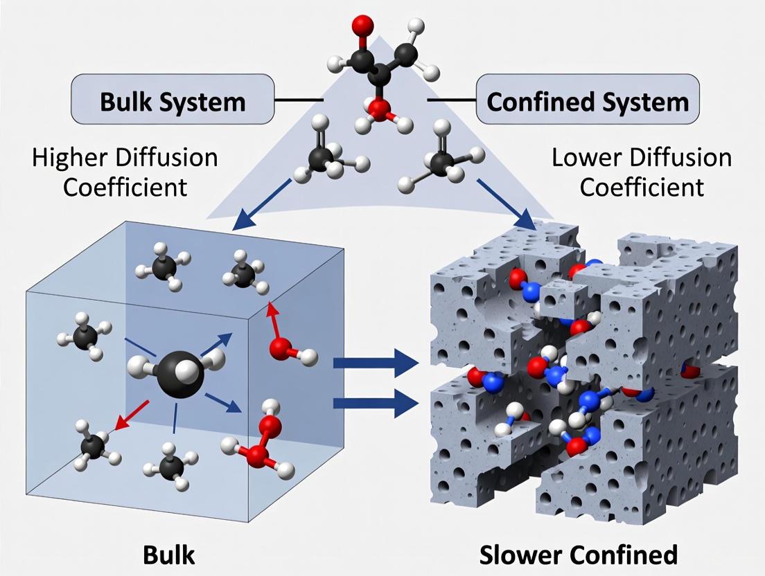
The behavior of diffusivity in bulk systems (unconfined, three-dimensional fluids) is traditionally well-characterized. However, in confined systems—where fluids are restricted at the nanoscale within porous materials, carbon nanotubes (CNTs), or nanochannels—the self-diffusion coefficient can deviate significantly from its bulk value [2] [3] [4]. This deviation arises from the complex interplay of factors such as fluid-wall interactions, the finite size of the confining geometry, and changes in the hydrogen-bonding network of fluids like water. The comparative study of diffusion in these two distinct environments provides critical insights for advancing technologies in nanomedicine, material science, and environmental engineering, where nanoconfined mass transfer is a pivotal process [2] [4].
Theoretical Frameworks: From Classical Relations to Entropy Scaling
The theoretical description of self-diffusion bridges macroscopic laws and microscopic dynamics. The classical Einstein relation (( D = \mu k_B T )) connects the macroscopic self-diffusion coefficient ( D ) to the microscopic mobility ( \mu ) of a particle, representing a fundamental application of the fluctuation-dissipation theorem [3]. This relationship holds for both bulk and confined systems, though the underlying dynamics may differ.
Recently, more advanced frameworks like entropy scaling have gained prominence. This approach posits that the reduced transport properties of fluids, including the self-diffusion coefficient, can be expressed as a monovariate function of the residual entropy [5]. This scaling is physically grounded and related to isomorph theory, providing a powerful tool for predicting diffusion coefficients across wide ranges of temperature and pressure, encompassing gaseous, liquid, and supercritical states. While initially developed for pure components, entropy scaling has been extended to model self-diffusion and mutual diffusion coefficients in mixtures in a thermodynamically consistent way, enabling predictions even for strongly non-ideal mixtures [5].
For confined systems, theoretical approaches often rely on kinetic theory and specialized equations that account for the geometric constraints imposed by the confining walls. For a hard-sphere fluid confined between parallel plates, a modified Boltzmann-Lorentz equation can be derived, leading to an explicit expression for the self-diffusion coefficient that depends on the system's height [6]. This theoretical prediction shows excellent agreement with molecular dynamics (MD) simulation results across a range of confinement sizes [6].
Experimental and Computational Methodologies
Accurately determining self-diffusion coefficients requires a combination of sophisticated experimental and computational techniques, each with its own strengths and applicable domains.
Experimental Techniques
- Nuclear Magnetic Resonance (NMR) with Field Gradients: This technique directly measures the macroscopic translational self-diffusion coefficient without requiring model-dependent analysis. It is unique in its ability to probe only translational motion, independent of rotational degrees of freedom, and is particularly valuable for studying supercooled water below the "no man's land" temperature range where crystallization hinders other techniques [3].
- Quasi-Elastic Neutron Scattering (QENS): QENS provides insights into microscopic translational dynamics by measuring the scattering of neutrons. It complements NMR by accessing a different time window (typically ( 10^{-8} ) to ( 10^{-14} ) seconds) and can probe the details of molecular motion, such as the relaxation of density fluctuations [3].
- Current Monitoring in Nanochannels: For ionic diffusion in nanochannels, a current monitoring method based on Fick's second law has been developed. This involves replacing the solution in reservoirs connected by a nanochannel and monitoring the ionic current during the diffusion process to extract the effective diffusion coefficient [4].
Computational Approaches
- Molecular Dynamics (MD) Simulations: MD is a primary computational tool that integrates classical equations of motion to generate time-resolved atomistic trajectories. Self-diffusion coefficients are typically calculated from the long-time slope of the mean-squared displacement (MSD) or, less commonly, from the velocity autocorrelation function [2] [7]. It is particularly valuable for confined systems where precise experimental control and measurement are challenging [2].
- Machine Learning and Symbolic Regression: Recent advances use machine learning, particularly symbolic regression (SR), to derive simple, physically consistent analytical expressions for self-diffusion coefficients. SR trains on MD simulation data to correlate diffusion coefficients with macroscopic variables like temperature, density, and pore size, bypassing the computationally expensive calculation of MSD [7] [8].
Diagram 1: Research workflow for comparing bulk and confined diffusion, integrating computational and experimental methods with machine learning and theoretical frameworks.
Quantitative Comparison: Bulk vs. Confined Self-Diffusion
The following tables summarize key quantitative relationships and data comparing self-diffusion in bulk and confined environments, synthesized from recent research.
Table 1: Summary of key parameters affecting self-diffusion in bulk and confined systems
| Parameter | Impact in Bulk Systems | Impact in Confined Systems | Key Experimental Evidence |
|---|---|---|---|
| Temperature | Linear increase with temperature [7] | Linear increase with temperature, but with a different slope [2] | MD simulations of SCW mixtures in CNTs (673-973 K) [2] |
| Density | Inversely proportional relationship [7] | Complex, system-dependent behavior | Symbolic regression analysis of molecular fluids [7] [8] |
| Pore Size | Not applicable | Increases with pore diameter, saturating to bulk value [2] [7] | MD studies of CNTs (diameter: 9.49-29.83 Å) [2] |
| Wall Chemistry | Not applicable | Hydrophilic confinement slows diffusion more than hydrophobic [3] | NMR/QENS studies of water in CNTs vs. MCM-41 [3] |
| Concentration | Varies with system | Remains relatively constant with varying solute concentration [2] | MD of SCW mixtures (solute concentration: 0.01-0.3) [2] |
Table 2: Representative mathematical models for predicting self-diffusion coefficients
| Model Type | System | Representative Equation | Performance/Notes |
|---|---|---|---|
| Symbolic Regression [7] | Bulk Fluids | ( D^{}_{SR} = \alpha_1 \frac{T^{\alpha2}}{\rho^{*\alpha3}} - \alpha_4 ) | ( R^2 > 0.98 ) for most of the nine molecular fluids studied |
| Entropy Scaling [5] | Pure & Mixture Fluids | ( \widehat{D} = f(s^{res}) ) | Enables prediction over wide state ranges including metastable states |
| Confinement Model [2] | CNT-confined SCW mixtures | Novel mathematical model based on CNT-solute relationship | Regression with ( R^2 = 0.9789 ) |
| Kinetic Theory [6] | Hard-sphere fluid between parallel plates | Explicit expression as a function of system height ( H ) | Very good agreement with MD simulations |
Research Reagent Solutions and Essential Materials
Table 3: Key research materials and computational tools for diffusion studies
| Material/Tool | Function/Application | Example from Research |
|---|---|---|
| Carbon Nanotubes (CNTs) | Model hydrophobic confinement system | Study of water and gas mixture diffusion [2] [3] |
| MCM-41 Silica Material | Model hydrophilic confinement system | Comparative studies with CNTs for water dynamics [3] |
| SPC/E Water Model | Molecular dynamics potential for water | Simulations of nano-confined water and binary mixtures [2] |
| Lennard-Jones Potential | Interatomic potential for MD simulations | Common choice for simplicity and computational efficiency [7] |
| Symbolic Regression Framework | Machine learning for deriving predictive equations | Correlating D with T, ρ, and H from MD data [7] [8] |
| KCl Electrolyte Solutions | Model system for ion diffusion studies | Measuring ion diffusion coefficients in nanochannels [4] |
The comparative analysis of self-diffusion coefficients in bulk versus confined systems reveals a complex landscape where nanoscale confinement significantly alters fundamental transport phenomena. While bulk diffusion follows relatively well-established relationships with temperature and density, confined diffusion exhibits additional dependencies on pore size, wall chemistry, and fluid-wall interactions. Experimental techniques like NMR and QENS, combined with advanced computational methods such as MD simulations and machine learning, provide complementary insights into these differences.
Emerging frameworks, including entropy scaling and symbolic regression, offer promising paths toward unified predictive models that can span both bulk and confined environments. These advances are not merely academic; they enable more efficient design of nanoscale confinement devices, improve theoretical understanding of fluid behavior under extreme conditions, and inform applications ranging from energy technology to drug delivery systems. Future research will likely focus on refining these models for more complex fluid mixtures and a wider variety of confining geometries, further closing the gap between our understanding of bulk and nanoconfined mass transfer.
The study of molecular motion under confinement is a critical area of research with profound implications across disciplines ranging from membrane separation and drug delivery to geochemistry and energy storage. When molecules reside within porous materials or near interfaces, their motion deviates significantly from the behavior observed in bulk solutions. These deviations are primarily governed by two key factors: the physical dimension of the confinement, typically represented by pore size, and the chemical nature of the confining surface. Understanding how these factors influence molecular diffusion provides fundamental insights into transport mechanisms at the nanoscale and enables the rational design of advanced materials for technological applications.
The interplay between confinement geometry and surface interactions creates a complex dynamic landscape. Pore size directly influences the entropy and available volume for molecular rearrangement, while surface chemistry dictates the energy landscape through which molecules navigate. Hydrophilic surfaces, characterized by polar groups or hydrogen-bonding capabilities, can strongly attract water molecules, potentially slowing their dynamics. In contrast, hydrophobic surfaces like carbon nanotubes (CNTs) may permit surprisingly fast transport due to minimal adhesion and the formation of vapor-like layers adjacent to the nonpolar walls [3]. This comparative guide examines the experimental and computational methodologies employed to quantify these effects and presents structured data illustrating how confinement alters molecular motion across different systems.
Comparative Data on Diffusion in Confined Systems
Quantitative Comparison of Diffusion Coefficients
The following tables consolidate experimental and simulation data from various studies, providing a direct comparison of molecular diffusion coefficients in bulk versus confined environments and illustrating the effects of pore size and surface chemistry.
Table 1: Water Self-Diffusion Coefficients in Bulk and under Confinement
| System | Temperature (K) | Pore Size/Diameter | Diffusion Coefficient (D) [m²/s] | Technique |
|---|---|---|---|---|
| Bulk Water [9] | ~300 | N/A | ~2.3 × 10⁻⁹ | Molecular Simulation |
| Hydrophilic MCM-41 [3] | ~250 | ~2.2 nm | ~1 × 10⁻¹¹ | NMR / QENS |
| Hydrophobic CNTs [3] | ~250 | ~1.5 nm | >1 × 10⁻⁹ | NMR / QENS |
| CNTs (Room Temp.) [2] | ~300 | 0.95 nm | ~8 × 10⁻⁹ | Molecular Dynamics (MD) |
| CNTs (Room Temp.) [2] | ~300 | 2.98 nm | ~4 × 10⁻⁹ | Molecular Dynamics (MD) |
Table 2: Effect of Confinement on Polymer Diffusion
| Polymer | Molecular Weight (g/mol) | Confinement Gap Height (μm) | Relative Diffusion Slowdown | Key Interaction |
|---|---|---|---|---|
| Dextran [10] | 70,000 | 21.8 (Near Bulk) | Baseline | Hydrodynamic resistance |
| Dextran [10] | 70,000 | 0.077 (High) | Significant slowdown | Hydrodynamic resistance |
| Sodium Polyacrylate [10] | ~450,000 | Varying | Slower diffusion near glass | Electrostatic/Surface adsorption |
Table 3: Solute Diffusion in Supercritical Water within CNTs
| Solute | Temperature (K) | CNT Diameter (Å) | Confined Self-Diffusion Coefficient [m²/s] | Key Energy Input Source |
|---|---|---|---|---|
| H₂ [2] | 673 - 973 | 9.49 - 29.83 | Increases linearly with temperature | >60% from CNT wall (Lennard-Jones) |
| CO₂ [2] | 673 - 973 | 9.49 - 29.83 | Saturation with increasing diameter | >60% from CNT wall (Lennard-Jones) |
| CH₄ [2] | 673 - 973 | 9.49 - 29.83 | Relatively constant with concentration | >60% from CNT wall (Lennard-Jones) |
Interpreting the Comparative Data
The data in Table 1 unequivocally demonstrates that confinement can either enhance or suppress molecular mobility depending on the surface interactions. The dramatically slower diffusion of water in hydrophilic MCM-41 silicas at supercooled temperatures, compared to bulk water, stems from strong hydrogen-bonding interactions with the pore walls [3]. In stark contrast, water confined within hydrophobic Carbon Nanotubes (CNTs) can exhibit remarkably fast transport, with diffusion coefficients approaching or even exceeding bulk values, a phenomenon attributed to the smooth, non-wetting nature of the graphene surface [3] [2].
Table 2 highlights that for larger, flexible molecules like polymers, confinement primarily leads to a slowdown in diffusion. This is largely due to increased hydrodynamic resistance as the polymer coils interact with the pore walls [10]. The extent of slowing depends on factors like polymer molecular weight, chain flexibility, and specific chemical interactions with the surface, such as electrostatic forces.
Table 3, based on Molecular Dynamics (MD) simulations of supercritical systems, reveals that for small gas molecules in CNTs, diffusion is strongly influenced by temperature and pore diameter, saturating as the pore becomes large enough to diminish wall-effects. Notably, over 60% of the energy input to solute molecules is derived from Lennard-Jones interactions with the CNT wall, underscoring the dominant role of the confining surface in energizing and facilitating molecular motion [2].
Experimental Protocols for Measuring Confined Diffusion
To generate the comparative data presented, researchers employ a suite of sophisticated experimental and computational techniques. Each method provides unique insights into different aspects of molecular motion, with characteristic spatial and temporal resolutions.
Nuclear Magnetic Resonance (NMR) in a Field Gradient
This technique is a benchmark for directly measuring the macroscopic translational self-diffusion coefficient (D) without requiring model-dependent analysis [3] [9].
- Core Principle: The protocol applies a linear magnetic field gradient across the sample. Molecular diffusion then causes a net displacement of spins, leading to an attenuation of the NMR signal. The rate of this attenuation is directly proportional to the self-diffusion coefficient, as described by the Stejskal-Tanner equation.
- Workflow:
- The porous material, saturated with the fluid of interest (e.g., water), is placed in the NMR spectrometer.
- A pulsed field gradient sequence is applied.
- The spin-echo signal is measured as a function of the gradient strength or pulse duration.
- The self-diffusion coefficient is extracted by fitting the signal decay.
- Key Advantage: It is insensitive to rotational motions and provides a direct, model-free measure of translational mobility over macroscopic distances (typically micrometers) [3].
Quasi-Elastic Neutron Scattering (QENS)
QENS complements NMR by probing microscopic translational dynamics on molecular length scales [3].
- Core Principle: The technique measures the energy broadening of neutrons scattered by the sample. This broadening, the "quasi-elastic" component, arises from the diffusive motion of atoms (e.g., hydrogen in water). The scattering function, S(Q,ω), is analyzed to extract the characteristic relaxation times and diffusion coefficients associated with different types of motion.
- Workflow:
- A beam of neutrons is directed at the confined fluid sample.
- The energy and momentum transfer of the scattered neutrons are analyzed.
- The QENS spectra are collected for a range of scattering vectors (Q).
- Models for molecular motion (e.g., jump diffusion, confined diffusion) are used to fit the S(Q,ω) data and derive the diffusion coefficient and residence times.
- Key Advantage: QENS can distinguish between different types of motion (e.g., localized rotation, long-range translation) and is sensitive to dynamics on time scales from 10⁻¹² to 10⁻⁸ seconds [3].
Convex Lens-Induced Confinement (CLiC) with Differential Dynamic Microscopy (DDM)
This is an advanced optical microscopy approach for studying soft matter and polymers in controlled confinement [10].
- Core Principle: A convex lens is placed on a coverslip, creating a sub-micrometer-thick, spatially varying gap. The diffusion of fluorescently labeled molecules within this gap is recorded by video microscopy. DDM analyzes the intensity fluctuations in the image series in Fourier space to extract the Intermediate Scattering Function (ISF), from which the diffusion coefficient is obtained.
- Workflow:
- The sample chamber is assembled with the lens and coverslip, creating a wedge-shaped gap.
- A solution of fluorescent polymers is introduced.
- Videos of the random motion of the molecules are captured at high frame rates.
- DDM processing is performed on the image stack to calculate the ISF.
- The relaxation rate of the ISF is plotted against the wave vector squared (q²), the slope of which yields the diffusion coefficient.
- Key Advantage: Allows high-throughput measurement of diffusion coefficients for a continuous range of confinement heights (from tens of nanometers to micrometers) in a single experiment, and is suitable for non-resolved particles [10].
Single-Molecule Tracking for Confinement Analysis
This technique is powerful for mapping transient confinement zones of molecules in complex biological environments, such as the plasma membrane [11].
- Core Principle: Individual molecules are labeled and imaged over time, generating trajectories of their precise positions. Algorithms then analyze these trajectories to detect periods where the molecule's motion deviates from a free random walk, indicating transient confinement in a "nanodomain."
- Workflow:
- Molecules of interest (e.g., membrane receptors) are labeled with bright, photostable fluorophores.
- Thousands of single-molecule trajectories are recorded with high spatial and temporal precision.
- A confinement index is calculated for each trajectory segment based on the probability that a Brownian particle would remain in a defined area for a given time.
- Segments with a confinement index exceeding a set threshold for a minimum duration are classified as confined.
- Confinement "hotspots" can be visualized relative to cellular structures.
- Key Advantage: Reveals heterogeneous diffusion and transient trapping events that are hidden in ensemble-averaged measurements [11].
Experimental Workflow and Confinement Mechanisms
The following diagrams illustrate the logical workflow of a typical confinement study and the fundamental physics governing molecular motion in pores.
Experimental Workflow for Confinement Studies
Diagram 1: Generalized workflow for experimental studies on molecular motion under confinement, highlighting key comparative stages.
Physics of Molecular Motion in a Confining Pore
Diagram 2: Key factors (surface interactions and pore size) influencing molecular motion in confinement, leading to either slowed or enhanced diffusion.
The Scientist's Toolkit: Key Reagents and Materials
Table 4: Essential Research Materials for Confined Diffusion Studies
| Material/Reagent | Function in Research | Example Application |
|---|---|---|
| Carbon Nanotubes (CNTs) | Model hydrophobic confining system with atomically smooth walls. | Studying fast water transport and ballistic diffusion [3] [2]. |
| MCM-41 Silica | Model hydrophilic confining material with tunable, cylindrical nanopores. | Investigating suppressed dynamics of supercooled water [3]. |
| Metal-Organic Frameworks (MOFs) | Highly tunable porous scaffolds with defined chemistry and topology. | Gas capture, separation, and studying adsorption selectivities [12]. |
| Dextran | Model flexible polymer ("foulant") for diffusion studies. | Understanding polymer dynamics in confinement relevant to membrane fouling [10]. |
| Fluorescent Dyes (e.g., TRITC, Alexa Fluor) | Labeling molecules for optical tracking and microscopy. | Enabling single-molecule tracking and Differential Dynamic Microscopy [10] [11]. |
| SPC/E Water Model | A classical molecular model for water used in simulations. | Simulating water structure and dynamics in bulk and confined environments [2]. |
Diffusion, the process by which molecules disperse from regions of high concentration to low concentration, is a fundamental transport mechanism in biological and synthetic nanoscale systems. However, the dynamics of this process are not uniform and are profoundly influenced by the environment. In nanoscale contexts, such as within biomolecular condensates or porous materials, classical Fickian diffusion often gives way to more complex, anomalous behaviors. Among these, ballistic diffusion has recently been identified as a distinct and efficient transport mode. This guide provides a comparative analysis of ballistic and Fickian diffusion, focusing on their characteristic dynamics, underlying mechanisms, and experimental signatures. Understanding these differences is critical for researchers and drug development professionals working to manipulate molecular transport in confined environments, such as targeted drug delivery systems or intracellular compartments.
Theoretical Framework: Defining the Diffusion Modes
Fickian Diffusion
Fickian, or normal, diffusion describes the random Brownian motion of particles in a homogeneous medium. It is governed by Fick's laws, which state that the flux of particles is proportional to the negative gradient of their concentration. A key signature of this mode is that the mean squared displacement (MSD) of the particles scales linearly with time (MSD ∝ t). In practical terms, this results in a blurry or fuzzy diffusion front that propagates with a square root of time dependence (ΔX ∝ t¹/²) [13]. This mode is dominant in simple, homogeneous fluids where particle movements are uncorrelated.
Ballistic Diffusion
In contrast, ballistic diffusion is characterized by a linear time dependence in its front propagation (ΔX ∝ t) [13]. This results in an ultrasharp, stable concentration front that moves with a constant velocity, akin to a wave. This behavior deviates from classical Brownian motion and arises when particle movements are persistent and highly correlated over time. Recent research on DNA-based biomolecular condensates has shown that this mode is enabled by molecular recognition (e.g., specific binding events like DNA hybridization) and a consequent phase transition within the condensate itself, from an arrested, solid-like state to a dynamic, liquid-like state [13] [14].
The table below summarizes the core differences between these two fundamental modes.
Table 1: Fundamental Characteristics of Ballistic and Fickian Diffusion
| Characteristic | Ballistic Diffusion | Fickian Diffusion |
|---|---|---|
| Propagation Kinetics | Linear with time (ΔX ∝ t) [13] | Square root of time (ΔX ∝ t¹/²) [13] |
| Front Morphology | Ultrasharp, stable front [13] | Fuzzy, gradient-based front [13] |
| Mean Squied Displacement | MSD ∝ t² (for single-particle motion) | MSD ∝ t |
| Primary Driver | Molecular recognition & phase transitions [13] | Concentration gradient |
| System State | Non-equilibrium steady state [13] | Equilibrium |
| Material Response | Can induce swelling and liquefaction [13] | Typically no structural change |
Experimental Evidence and Quantitative Data
The distinct nature of ballistic diffusion has been quantitatively demonstrated in controlled experimental systems, providing clear data for comparison.
Model System: DNA Biomolecular Condensates
A key study utilized core-shell condensates formed from long single-stranded DNA (ssDNA) copolymers. The core contained addressable barcode sequences (m), which served as binding sites for complementary short oligonucleotides, termed "invaders" (m*) [13]. When these fluorescently labelled invaders were introduced, they did not diffuse randomly. Instead, they formed a sharp, high-intensity front that propagated linearly into the condensate. This front coincided with a boundary between the non-invaded, compact core and a swollen, invaded region, which expanded the condensate volume approximately fourfold [13].
Comparative Dynamics and Material Properties
The invasion process did more than just transport molecules; it fundamentally altered the physicochemical properties of the condensate. The following table integrates quantitative data from various analytical techniques, comparing the state of the condensate before and after the ballistic invasion front passed through.
Table 2: Experimental Data from DNA Condensate Studies Comparing Non-Invaded and Invaded Regions
| Analysis Method | Non-Invaded (Arrested) State | Invaded (Dynamic) State | Implication |
|---|---|---|---|
| Fluorescence Recovery After Photobleaching (FRAP) | No recovery after 6,000 seconds (arrested dynamics) [13] | Full fluorescence recovery (dynamic state) [13] | Liquefaction and transition to a fluid-like environment post-invasion. |
| Reciprocal Half-Recovery Time (1/t₁/₂) | ~0.00017 s⁻¹ (very slow) [13] | ~0.02 s⁻¹ (≥100x faster) [13] | Quantifies a difference in mobility of at least two orders of magnitude. |
| Fluorescence Lifetime Imaging (FLIM) | Lifetime ~2.9 ns [13] | Lifetime ~3.4 ns [13] | Indicates a change in the local molecular environment and polymer chain flexibility. |
| Atomic Force Microscopy (AFM) | Stiffer, elastic response; little hysteresis [13] | Softer, larger hysteresis (energy dissipation) [13] | Confirms a mechanical transition from solid-like to liquid-like viscoelasticity. |
| Final Swelling Ratio | - | ~4x volume increase [13] | Direct evidence of structural expansion driven by molecular recognition. |
This dataset provides a multi-faceted validation of the ballistic diffusion mechanism and its profound impact on the nanoscale environment. For comparison, the effective diffusion coefficient in shale rock with nano-confinement, a system likely dominated by anomalous diffusion, can be reduced by 10² to 10⁴ times compared to bulk phase diffusivity as porosity decreases [15].
Detailed Experimental Protocols
To ensure reproducibility and provide a clear technical roadmap, this section outlines the key methodologies used to generate the data on ballistic diffusion.
Protocol 1: Establishing the DNA Condensate Model and Invader Assay
This protocol details the preparation of the biomolecular condensates and the initial invasion experiment [13].
Condensate Formation:
- Materials: Prepare a mixture of two long ssDNA copolymers, p(A20-m)n and p(T20-k)n, in a TE buffer containing 50 mM MgCl₂.
- Phase Separation: Heat the mixture above the cloud point temperature of p(A20-m)n (~42°C) to induce liquid-liquid phase separation and form spherical condensates.
- Shell Formation: During cooling, allow p(T20-k)n to localize at the condensate periphery via A20/T20 hybridization, forming a core-shell structure.
- Visualization: Label the shell's k barcodes with a fluorescent ssDNA strand (k*-dye) for visualization under a fluorescence microscope.
Invasion and Imaging:
- Introduction of Invader: Add the complementary invader strand (m*-Atto488) to the condensate solution.
- Time-Lapse Imaging: Use confocal fluorescence microscopy to capture the uptake of the invader over time. Specifically, monitor the formation and propagation of the sharp fluorescence front.
- Swelling Quantification: Measure the change in condensate volume by tracking the boundary of the core material before and after invasion.
Protocol 2: Probing Condensate Dynamics via FRAP and FLIM
This protocol describes how to characterize the dynamic state of the condensate in different regions [13].
Fluorescence Recovery After Photobleaching (FRAP):
- Pre-invasion Measurement: Select a region of interest (ROI) within a non-invaded condensate and bleach the fluorescence using a high-intensity laser pulse.
- Recovery Monitoring: Record the fluorescence intensity within the bleached ROI over time (e.g., 6,000 seconds) to assess mobility.
- Post-invasion Measurement: Repeat the bleaching and monitoring process within a region of the same condensate after the invader front has passed through.
- Quantification: Fit the recovery curves to calculate the half-recovery time (t₁/₂) and its reciprocal (1/t₁/₂) for quantitative comparison.
Fluorescence Lifetime Imaging (FLIM):
- Image Acquisition: Acquire fluorescence lifetime images of the condensates, ensuring to capture both invaded and non-invaded regions.
- Lifetime Analysis: For each pixel, determine the fluorescence decay lifetime. Plot the data on a phasor plot to visually distinguish the lifetime distributions of the two states.
- Comparison: Calculate the average lifetime in the non-invaded (arrested) region versus the invaded (dynamic) region.
Protocol 3: Assessing Mechanical Properties with AFM
This protocol measures the nanomechanical properties changes associated with the diffusion mode [13].
- Sample Preparation: Immobilize DNA condensates on a suitable substrate for AFM measurement.
- Force Spectroscopy: Use a colloidal probe AFM tip to perform indentation experiments on both non-invaded and invaded condensates.
- Data Collection: Record force-distance curves during the compression and retraction cycles.
- Analysis:
- Elasticity: Compare the slope of the force curve during indentation; a steeper slope indicates a stiffer, more elastic material.
- Dissipation: Calculate the hysteresis (area between the compression and retraction curves) as a measure of energy dissipation, which is characteristic of liquid-like materials.
Signaling Pathways and Workflow Visualizations
The following diagrams illustrate the logical relationship between the two diffusion modes and the specific experimental workflow used to study ballistic wave diffusion.
The Scientist's Toolkit: Essential Research Reagents and Materials
Successful research into nanoscale diffusion dynamics requires a specific set of tools. The following table lists key reagents, materials, and instruments used in the featured studies.
Table 3: Essential Research Reagents and Solutions for Diffusion Studies
| Category | Item | Specific Example / Function | Key Application |
|---|---|---|---|
| Model System Components | ssDNA Copolymers | p(A20-m)n and p(T20-k)n; form the scaffold of the biomolecular condensate [13]. | Core material for creating model biomolecular condensates. |
| Invader Oligonucleotide | m*-Atto488; complementary strand that binds to core barcodes, enabling molecular recognition [13]. | Probe for studying ballistic wave diffusion. | |
| Divalent Salt Solution | MgCl₂ in TE buffer; essential for coacervation and condensate formation [13]. | Condensate formation and stability. | |
| Imaging & Analysis | Confocal Microscope | Equipped with environmental control; for time-lapse imaging of front propagation [13]. | Visualizing and quantifying diffusion front kinetics. |
| FRAP/FLIM Module | Attached to microscope; measures molecular mobility and local environment [13]. | Probing condensate dynamics and polymer chain flexibility. | |
| Atomic Force Microscope | With colloidal probe; performs nanoindentation to measure viscoelasticity [13]. | Characterizing mechanical properties (stiffness, dissipation). | |
| Specialized Reagents | Fluorescent Dyes | Atto488, Atto594; label oligonucleotides for visualization [13]. | Fluorescent tagging for microscopy. |
| Peptide Nucleic Acid (PNA) | m*PNA-Atto488; neutral backbone control for invader experiments [13]. | Control experiments to isolate effects of molecular recognition. |
This comparison guide delineates the fundamental differences between ballistic and Fickian diffusion modes in nanoscale environments. While Fickian diffusion remains a cornerstone of transport theory, the emergence of ballistic diffusion, characterized by its sharp front and linear propagation, represents a significant advancement in our understanding. The critical differentiator is the role of molecular recognition, which not only drives transport but also actively remodels the nanoscale environment, inducing phase transitions and altering material properties. For researchers in drug delivery and nanomedicine, where penetrating dense tissues or targeting specific intracellular compartments is a major hurdle, the principles of ballistic diffusion could inform the design of next-generation delivery systems. By engineering carriers that leverage specific binding and environment-remodeling capabilities, it may be possible to achieve deeper and more precise tissue penetration, moving beyond the limitations imposed by classical diffusion.
The behavior of molecules under nanoscale confinement differs dramatically from their properties in bulk solutions, a phenomenon of critical importance in fields ranging from drug delivery to membrane technology. The nature of the confining material itself—whether hydrophobic like carbon nanotubes (CNTs) or hydrophilic like porous silica (MCM-41)—governs fundamental molecular processes, particularly diffusion. Within the context of comparing bulk versus confined system diffusion coefficients, this guide objectively examines how these two distinct environments impact the translational mobility of confined substances, with water as a principal model system. Understanding these differences enables researchers to select confinement materials strategically to achieve desired transport properties in applications such as controlled drug release, catalytic reactions, and analytical sensors.
Fundamental Concepts and Key Differences
Hydrophobic and hydrophilic confinements exert their influence primarily through their distinct interactions with water molecules, which in turn structure the confined water and dictate its mobility.
- Hydrophobic Confinement (e.g., Carbon Nanotubes - CNTs): Characterized by non-polar, water-repelling surfaces, hydrophobic confinement favors interactions between the water molecules themselves. This can lead to the formation of vapor-like layers or streamlined water networks that minimize contact with the confining walls. The resulting reduced friction often leads to significantly enhanced self-diffusion coefficients compared to bulk water, a phenomenon often described as "fast water transport" [3] [16].
- Hydrophilic Confinement (e.g., MCM-41): Featuring polar, water-attracting surfaces rich in silanol (Si-OH) groups, hydrophilic confinement promotes strong hydrogen-bonding interactions between the water molecules and the pore walls. These interactions can restrict water mobility by pinning molecules to the surface, disrupting the bulk hydrogen-bond network, and leading to a reduced self-diffusion coefficient compared to bulk water, especially at lower temperatures [3] [16].
The divergence in dynamics is most pronounced in the supercooled state, a metastable liquid phase below the freezing point, where the properties of bulk water are notoriously difficult to study due to crystallization. Confinement suppresses ice formation, allowing investigation within this "no man's land" [3] [16].
Figure 1: Conceptual workflow for analyzing diffusion in hydrophobic versus hydrophilic confinement, linking material choice to interaction mechanisms and final outcomes.
Experimental Protocols for Measuring Confined Diffusion
Accurately assessing the diffusion of molecules in confinement requires techniques that can probe dynamics across different length and time scales. The following table summarizes the core methodologies employed in this field.
Table 1: Key Experimental Techniques for Measuring Diffusion in Confinement
| Technique | Measured Property | Spatial/Temporal Scope | Primary Application in Confinement Studies |
|---|---|---|---|
| Pulsed-Field Gradient NMR (PFG-NMR) [3] [16] | Macroscopic translational self-diffusion coefficient (D) | Macroscopic scale; ~100 to 10⁻¹⁰ s [16] | Directly measures the mean square displacement of molecules over large distances without model-dependent analysis. |
| Quasi-Elastic Neutron Scattering (QENS) [3] [16] | Microscopic translational dynamics & relaxation times | Microscopic scale; ~10⁻⁸ to 10⁻¹⁴ s [16] | Probes single-particle motion (self-diffusion) and collective dynamics on molecular length scales, providing insights into localized mobility. |
| Heterodyne-Detected Sum-Frequency Generation (HD-SFG) [17] | Molecular orientation & hydrogen-bond environment at interfaces | Interface-specific, sub-nm depth; vibrational timescales | Selectively probes the structure and orientation of water molecules at the confining wall interface, distinguishing between hydrophobic and hydrophilic effects. |
The synergy between NMR and QENS is particularly powerful, as they provide complementary macroscopic and microscopic views of molecular motion, offering a complete picture from local jumps to long-range transport [3] [16].
Comparative Data: Hydrophobic CNTs vs. Hydrophilic MCM-41
The distinct interaction mechanisms result in quantifiably different diffusion behaviors. The following table synthesizes experimental findings comparing water dynamics in these two environments.
Table 2: Comparative Dynamics of Water in Hydrophobic CNT vs. Hydrophilic MCM-41 Confinement
| Characteristic | Hydrophobic Confinement (CNTs) | Hydrophilic Confinement (MCM-41) |
|---|---|---|
| Self-Diffusion Coefficient (D) | Enhanced relative to bulk water [3] [16]. Extraordinarily fast transport has been observed [16]. | Reduced relative to bulk water, especially at lower temperatures [3] [16]. |
| Primary Cause of D Change | Smooth molecular walls & minimized water-wall friction; strong water-water H-bonding promotes collective, bulk-like flow [3] [16]. | Strong hydrogen-bonding interactions between water and the polar silica surface (pinning effect) [3] [16]. |
| Hydrogen Bond Network | Preserved or optimized internally among water molecules [3]. | Disrupted and reorganized by the hydrophilic pore walls [3]. |
| Temperature Dependence in Supercooled Regime | Dynamics remain relatively faster, aiding the study of supercooled water [3] [16]. | Marked slowing of dynamics, revealing a more pronounced departure from bulk behavior [3] [16]. |
| Theoretical/Simulation Support | Attributed to vapor layer formation & low friction [3]. Molecular dynamics simulations support fast flow [3]. | AIMD simulations and experimental data align with ordered interfacial water and slowed dynamics [17]. |
The Scientist's Toolkit: Essential Research Reagents and Materials
Research into confined diffusion relies on well-characterized materials and specialized instruments. Below is a list of key resources used in the experiments cited in this guide.
Table 3: Essential Research Materials and Tools for Confined Diffusion Studies
| Item Name | Function/Description | Example Application/Context |
|---|---|---|
| Carbon Nanotubes (CNTs) | Model system for smooth, hydrophobic confinement [3] [16]. | Studying fast water transport and enhanced self-diffusion [3] [16]. |
| MCM-41 (Mesoporous Silica) | Model system for ordered, hydrophilic confinement with tunable, cylindrical nanopores [3] [16]. | Investigating the effect of surface polarity and pore size on water dynamics [3] [16]. |
| Pulsed-Field Gradient NMR Spectrometer | Instrument for directly measuring the macroscopic translational self-diffusion coefficient (D) [3] [16]. | Quantifying the average diffusion rate of water molecules in CNT or MCM-41 pores over macroscopic distances [3] [16]. |
| Quasi-Elastic Neutron Scattering (QENS) Spectrometer | Instrument for probing microscopic translational and rotational dynamics on molecular length scales [3] [16]. | Analyzing the localized motion and relaxation times of water confined in nanopores [3] [16]. |
| HD-SFG Spectrometer | Surface-specific vibrational spectrometer for probing molecular orientation and H-bond environment at interfaces [17]. | Elucidating the structure of water at the confining wall interface under angstrom-scale confinement [17]. |
The choice between hydrophobic and hydrophilic confinement materials is not merely a technical detail but a fundamental design parameter that dictates the diffusional behavior of confined molecules. As the comparative data demonstrates, hydrophobic materials like CNTs can enhance molecular diffusion, while hydrophilic materials like MCM-41 typically suppress it. This distinction is critical for researchers and drug development professionals designing nanocarrier systems, catalytic reactors, or separation membranes where controlled molecular transport is paramount.
Future research directions will likely focus on engineering composite and smart confinement materials that leverage both hydrophobic and hydrophilic motifs to achieve even finer control over diffusion. Furthermore, the integration of advanced techniques like HD-SFG [17] with traditional methods (NMR, QENS) will continue to deepen our molecular-level understanding, ultimately enabling the rational design of confined systems for specific biomedical and industrial applications.
The diffusion coefficient (D) is a fundamental physicochemical parameter that governs the spontaneous transport of molecules, playing a critical role in processes ranging from drug delivery in biological systems to catalytic reactions in industrial reactors [18] [19] [20]. For researchers and drug development professionals, accurately predicting and measuring diffusion coefficients is essential for understanding bioavailability, biodistribution, and optimizing delivery systems [21] [20]. The theoretical framework for describing molecular diffusion has evolved significantly from classical hydrodynamic equations to sophisticated modern computational models, each with distinct advantages and limitations, particularly when comparing bulk fluid environments with nanoconfined systems [3] [22]. This guide provides an objective comparison of these theoretical frameworks, supported by experimental data and detailed methodologies, to inform selection and application in research and development contexts.
Fundamental Theoretical Frameworks
The Stokes-Einstein Equation: Foundation and Assumptions
The Stokes-Einstein equation represents the foundational theory for describing particle diffusion in liquids. This 117-year-old equation relates the diffusion coefficient of a spherical particle to the temperature and viscosity of its surrounding medium [18] [23]:
D = kBT / (6πrη0)
Where D is the diffusion coefficient, kB is Boltzmann's constant, T is absolute temperature, r is the hydrodynamic radius of the particle, and η0 is the solvent viscosity [18]. Originally derived for Brownian motion in simple liquids, this equation provided early empirical evidence for the reality of atoms and molecules [23]. The equation assumes: (1) spherical particles, (2) continuum solvent mechanics, (3) no solute-solvent interactions beyond hydrodynamic drag, and (4) applicability to infinite dilution conditions [18] [24]. While remarkably enduring, these assumptions become problematic in complex biological and confined environments where molecular shapes are irregular and concentrations are high [24] [23].
Modified Stokes-Einstein Equations for Complex Systems
For non-spherical particles and concentrated systems, modifications to the classical Stokes-Einstein equation have been proposed. A significant advancement incorporates effective viscosity to account for molecular crowding:
D = kBT / (6πrηeff)
Where ηeff represents an effective viscosity that depends on the volume fractions (ϕi) of all molecular species in the system [24]. This modification addresses the key shortcoming that "the SE relation takes the viscosity to be a constant, based upon the solvent viscosity," when in reality, "it should depend upon the concentration of the various species of molecules present in the system" [24]. For protein aggregation systems like Aβ aggregation implicated in Alzheimer's disease, further modifications incorporate shape factors for non-spherical particles, recognizing that "aggregates of Aβ peptide cannot be assumed to be spherical" [24].
Modern Computational Approaches
Machine learning (ML) models represent a paradigm shift in predicting diffusion coefficients for complex fluids. Recent research demonstrates that ML models can predict diffusion coefficients and ionic conductivity of bulk and nanoconfined ionic liquids over wide temperature ranges (350-500 K) using simple physical descriptors of cations and anions such as molecular weight and surface area [22]. These models offer "fast and computationally efficient" alternatives to "expensive molecular dynamics simulations" and can be trained on molecular dynamics simulation data for numerous ionic liquids as bulk fluids and confined in graphite slit pores [22]. Importantly, accurate results can be obtained using only descriptors derived from SMILES (simplified molecular-input line-entry system) codes for the ions with minimal computational effort [22].
Table 1: Comparison of Theoretical Frameworks for Diffusion Coefficients
| Framework | Fundamental Principles | Optimal Application Domain | Key Limitations |
|---|---|---|---|
| Classical Stokes-Einstein | Relates D to spherical radius and solvent viscosity | Dilute solutions in bulk fluids; spherical molecules | Fails for non-spherical particles; inaccurate in confined systems and high concentrations |
| Modified Stokes-Einstein | Incorporates effective viscosity and shape factors | Crowded environments; protein aggregation systems; non-spherical molecules | Requires knowledge of volume fractions and molecular dimensions |
| Machine Learning Models | Learns D from molecular descriptors and simulation data | Bulk and confined ionic liquids; high-throughput screening | Dependent on quality and breadth of training data; limited transferability |
| Molecular Modeling | Calculates molecular radius from stable conformers | Small molecule drugs; drug screening applications | Accuracy depends on hydration effects and conformational sampling |
Comparative Performance: Bulk vs. Confined Systems
Experimental Evidence in Hydrophobic vs. Hydrophilic Confinement
The behavior of confined water provides compelling experimental evidence for the drastically different diffusion properties in confined versus bulk environments. Research demonstrates that "confined water is a model system for the study of supercooled water" and that "the accurate assessment of the translational mobility of water molecules, especially in the supercooled state, can unmistakably distinguish between the hydrophilic and hydrophobic nature of the confining environments" [3]. Using Nuclear Magnetic Resonance (NMR) and quasi-elastic neutron scattering (QENS), studies have shown that water confined in hydrophobic carbon nanotubes (CNTs) exhibits "extraordinarily fast transport" compared to bulk water, while water in hydrophilic MCM-41 materials shows different dynamic behavior [3]. This difference has been attributed to "the strong hydrogen bonding between water molecules, which can cause the liquid to recede from nonpolar surfaces to form a vapor layer separating the bulk phase from the surface" in hydrophobic confinement [3].
Quantitative Comparisons Across Environments
Table 2: Experimental Diffusion Coefficients in Different Environments
| Molecular System | Environment | Temperature | Diffusion Coefficient (cm²/s) | Measurement Technique |
|---|---|---|---|---|
| Water | Bulk (supercooled) | Below 230 K | Unmeasurable (crystallization) | NMR [3] |
| Water | Hydrophobic CNT confinement | Below 230 K | Measurable (fast transport) | NMR, QENS [3] |
| Water | Hydrophilic MCM-41 confinement | Below 230 K | Measurable (slower than CNT) | NMR, QENS [3] |
| Theophylline | Artificial mucus | 25°C | 6.56 × 10⁻⁶ | FTIR [21] |
| Albuterol | Artificial mucus | 25°C | 4.66 × 10⁻⁶ | FTIR [21] |
| Ionic Liquids | Graphite slit pores | 350-500 K | ML-predicted values | Molecular Dynamics [22] |
Validity in Biological Systems
Recent research has defended the validity of the Stokes-Einstein equation in complex biological environments. Studies working with proteins in live bacteria found that "although Einstein's equation appeared to be off for proteins' motion within live bacteria, it remained valid by taking into account the entangled polymers and filaments inside bacteria" [23]. This research revealed that bacterial cytoplasm, rather than being "a simple soup," might be more like "spaghetti with tomato sauce and meatballs," emphasizing the importance of accounting for molecular crowding [23]. This finding has significant implications for understanding antibiotic resistance and the mechanical properties of cancer cells, which "differ from the mechanical properties of normal, healthy cells" [23].
Experimental Methodologies for Validation
Spectroscopic Techniques
Fourier Transform Infrared Spectroscopy (FTIR) provides a non-invasive method for determining drug diffusion coefficients through complex media like artificial mucus. In this approach, "the upper surface of a mucus layer is placed in contact with the drug solutions and the lower mucus surface is in contact with a zinc selenide crystal to allow for time-resolved FTIR measurements" [21]. FTIR spectra are collected at constant time intervals and monitored for quantitative changes in spectral peaks corresponding to functional groups specific to each drug. Changes in peak heights are correlated to concentration via Beer's Law, and Fick's 2nd Law of Diffusion is used along with Crank's trigonometric series solution for a planar semi-infinite sheet to analyze the concentration data and determine diffusion coefficients [21].
NMR and QENS Approaches
Nuclear Magnetic Resonance (NMR) in a field gradient "directly measures the macroscopic translational self-diffusion coefficient D without using a model-dependent analysis," while quasi-elastic neutron scattering (QENS) "can determine the microscopic translational dynamics of the water molecules" [3]. These techniques complement each other with time scale sensitivities of about 100 to 10⁻¹⁰ seconds for NMR and 10⁻⁸ to 10⁻¹⁴ seconds for QENS [3]. The combination of these techniques "could provide a more accurate analysis of the molecular motions" of specific systems, particularly in the deep supercooled region of water where differences in translational dynamics between bulk and confined systems become clearly observable [3].
Fluorescence-Based Methods
A simple method using fluorescence intensity measurements with a microplate reader can determine diffusion coefficients in soft hydrogels for drug delivery applications. This approach involves analyzing "the diffusion behavior of three fluorescent particles of different chemical natures and various molecular weights in agarose hydrogels of low percentages (0.05-0.2%)" [25]. The diffusion coefficients are obtained by fitting the experimental data to a one-dimensional diffusion model, and the method can adapt "to hydrogels of different stiffnesses and solutes of various sizes and characteristics" [25]. The combination of hydrogel sectioning with multiple simultaneous measurements in a microplate reader shows the simplicity of the experimental procedure [25].
Essential Research Reagents and Materials
Table 3: Key Research Reagent Solutions for Diffusion Experiments
| Reagent/Material | Function in Diffusion Studies | Example Applications |
|---|---|---|
| Artificial Mucus | Models physiological barrier for drug transport | Asthma drug diffusion studies (theophylline, albuterol) [21] |
| Agarose Hydrogels | Creates controlled porous environment for diffusion | Protein and nanoparticle penetration studies [25] |
| Carbon Nanotubes | Provides hydrophobic confinement environment | Studying fast water transport mechanisms [3] |
| MCM-41 Silica | Provides hydrophilic confinement environment | Comparative studies of hydrophobic vs hydrophilic effects [3] |
| Ionic Liquids | Model complex fluids for confinement studies | Machine learning model training for diffusion prediction [22] |
| Fluorescent Tracers | Enables visualization and quantification of diffusion | Fluorescein, mNeonGreen, BSA for hydrogel studies [25] |
The evolution from the classical Stokes-Einstein equation to modern molecular models reflects the growing complexity of systems being studied—from simple bulk fluids to biologically relevant confined environments. The Stokes-Einstein equation remains fundamentally valid when properly modified to account for molecular crowding, shape factors, and confinement effects [24] [23]. For drug development professionals, understanding these frameworks is essential for predicting drug behavior in physiological environments, where barriers like mucus and cellular compartments create natural confinement effects [21] [20]. The emergence of machine learning approaches offers promising avenues for high-throughput screening of diffusion properties in drug candidate molecules, potentially providing "an additional molecular property in drug screening" [18]. As research continues, integrating these complementary theoretical frameworks with robust experimental validation will enhance our ability to predict and optimize molecular transport in increasingly complex environments.
Measuring and Modeling Diffusion: From Molecular Simulations to Drug Delivery Applications
Molecular diffusion, the process by which molecules spread from regions of high concentration to low concentration through random motion, is a fundamental process underpinning numerous scientific and industrial applications. In drug development, the efficacy of an inhaled therapeutic depends on its ability to diffuse through the mucus barrier in the lungs to reach the target site [26]. In chemical engineering, the efficiency of a reactor producing sorbitol from glucose hinges on the accurate knowledge of the diffusion coefficients of the reacting species [19]. Similarly, in materials science, the performance of rejuvenators used to repair aged bitumen in roads is governed by their diffusivity within the material [27]. Accurately calculating diffusion coefficients (D) is therefore not merely an academic exercise but a critical requirement for rational design and optimization across these fields.
Molecular Dynamics (MD) simulation has emerged as a powerful computational technique to study diffusion at the atomic level. It provides a dynamic view of molecular motion, offering insights that are often difficult or impossible to obtain through experimental means alone. This guide provides a objective comparison of the performance of MD simulations for calculating diffusion coefficients, with a specific focus on the critical distinction between bulk and spatially confined systems. We will summarize quantitative performance data, detail essential experimental protocols, and provide a toolkit for researchers to apply these methods effectively.
MD Simulation Fundamentals: Theory and Key Protocols
Theoretical Underpinnings of Diffusion in MD
At its core, molecular diffusion in a viscous environment is described by Fick's laws. Fick's first law states that the flux of molecules is proportional to the negative of the concentration gradient, with the diffusion coefficient D as the proportionality constant [28]. The continuum-level description of diffusion is captured by Fick's second law (or the diffusion equation), which describes how the concentration changes over time [28] [26].
MD simulations leverage a particle-based perspective to access these properties. The primary method for calculating the self-diffusion coefficient in an MD simulation is the Einstein relation, which connects the macroscopic diffusion coefficient to the mean square displacement (MSD) of the molecules over time [28]:
<∣r − r0∣²> = 2nDt
Here, <∣r − r0∣²> is the ensemble-averaged MSD, n is the dimensionality (typically 3), and t is time. Thus, D is calculated as one-sixth of the slope of the MSD versus time plot in three dimensions [28]. An alternative, theoretically equivalent approach is the Green-Kubo relation, which integrates the velocity autocorrelation function of the molecules [28].
Standardized MD Protocol for Diffusion Coefficients
A typical MD workflow for determining a diffusion coefficient involves several key stages, which are compared for bulk and confined systems in the diagram below.
System Preparation: For a bulk system, the molecules of interest are placed in a cubic simulation box with periodic boundary conditions applied in all three dimensions to mimic an infinite system [28]. For a confined system, rigid walls are introduced in one or more dimensions, breaking the periodicity in those directions. The wall atoms are typically fixed in their lattice sites and have specific interaction parameters with the fluid molecules [29].
Equilibration: The system is first equilibrated for a duration several times longer than the system's longest relaxation time (τ) to ensure it reaches a true thermodynamic equilibrium at the target temperature and pressure. For confined polymer melts, this is when interfacial chains adopt mostly "L" or "U"-shaped configurations on the wall surfaces [29].
Production Run and Analysis: A longer production simulation is then performed to collect trajectory data. The MSD is calculated for the molecules, and D is derived from its slope. A critical finding is that for solutes in solution, a strategy of averaging the MSD from multiple short simulations can be more efficient for achieving reliable statistics than a single, very long simulation [28].
Performance Comparison: MD vs. Experiment and Between Systems
Quantitative Accuracy of MD Predictions
The true test of a computational method is its validation against experimental data. The following table summarizes the performance of the General AMBER Force Field (GAFF) in predicting diffusion coefficients for various systems, demonstrating that MD can achieve remarkable accuracy and correlation with experiments.
Table 1: Performance of GAFF Force Field in Predicting Diffusion Coefficients [28]
| System Type | Number of Systems Tested | Average Unsigned Error (AUE) (×10⁻⁵ cm²/s) | Root-Mean-Square Error (RMSE) (×10⁻⁵ cm²/s) | Correlation with Experiment (R²) |
|---|---|---|---|---|
| Organic Solutes in Aqueous Solution | 5 | 0.137 | 0.171 | Not Specified |
| Organic Solvents | 8 | Not Specified | Not Specified | 0.784 |
| Proteins in Aqueous Solutions | 4 | Not Specified | Not Specified | 0.996 |
| Organic Compounds in Non-Aqueous Solutions | 9 | Not Specified | Not Specified | 0.834 |
Beyond the performance of a specific force field, direct study-by-study comparisons show that MD simulations can yield results that align closely with experimental values in both magnitude and trend.
Table 2: Direct Experimental Validation of MD Simulations Across Applications
| Application Context | MD-Predicted D (m²/s) | Experimentally Measured D (m²/s) | Key Finding |
|---|---|---|---|
| Rejuvenators in Aged Bitumen [27] | 10⁻¹¹ to 10⁻¹⁰ | ~10⁻¹¹ to 10⁻¹⁰ | Excellent agreement in both magnitude and order (BO > EO > NO > AO). |
| Drugs in Aqueous Solution [30] | Anhydrous Carbamazepine: ~7.4 × 10⁻¹⁰ | ~7.4 × 10⁻¹⁰ | MD and UV imaging method produced identical results. |
| Polymers in Bulk Melt [29] | C₅₀ PE Melt at 450K | N/A (Study focused on mechanism) | Successfully characterized chain tumbling and rotation mechanisms. |
The Bulk vs. Confined System Divide
A central theme in diffusion research is the stark contrast between bulk and confined environments. MD simulations are exceptionally powerful in elucidating these differences at the molecular level.
- Bulk System Dynamics: In a bulk polymer melt under shear, chains first align and then stretch as flow strength increases. At intermediate flow, they exhibit symmetrical S-shaped rotations and tumbling. Under strong flow, this motion becomes asymmetric, with chains tumbling quickly in a hairpin-like configuration [29].
- Confined System Dynamics: Near a solid wall, the dynamics change dramatically. Interfacial chains have segments adsorbed to the wall and others detached. This dual state leads to distinctive molecular mechanisms, as the adsorbed segments experience direct wall friction while the non-adsorbed segments interact with the surrounding fluid [29]. This results in a longer characteristic relaxation time for confined melts (e.g., 26.7 ns for C178 confined PE vs. 15.6 ns for its bulk counterpart) [29], which directly impacts the diffusivity and rheological response.
Table 3: Key Research Reagent Solutions for MD Simulations of Diffusion
| Item / Resource | Function / Description | Example Use Case |
|---|---|---|
| General AMBER Force Field (GAFF) | A force field designed for organic molecules, providing parameters for most drugs and small molecules. | Predicting diffusion coefficients of organic solutes and proteins in aqueous solution [28]. |
| Siepmann-Karaboni-Smit Model | A united-atom model for simulating polyethylene melts, where CH₂ and CH₃ groups are treated as single interaction sites. | Studying chain dynamics of polyethylene melts in bulk and under confinement [29]. |
| p-SLLOD Algorithm | An algorithm for implementing shear flow in non-equilibrium MD simulations. | Subjecting polymer melts to simple shear flow to study rheology and chain dynamics [29]. |
| Nosé–Hoover Thermostat | A method to maintain a constant temperature during MD simulations, ensuring correct thermodynamic sampling. | Temperature control in simulations of polymer melts under shear [29]. |
| r-RESPA (Reversible Reference System Propagator Algorithm) | A multiple time-step algorithm for integrating motion, allowing longer time steps for slower interactions. | Efficiently simulating large polymer systems by using a short time step for bonded interactions and a longer one for nonbonded forces [29]. |
Molecular Dynamics simulations have firmly established themselves as computational powerhouses for the calculation of diffusion coefficients. As validated by experimental data, they offer not only quantitative accuracy but also unparalleled molecular-level insight into dynamic processes. The forced field performance data and validation cases presented here give researchers a clear benchmark for what can be achieved.
A critical insight from modern research is that the choice between modeling a bulk or a confined system is not trivial—it fundamentally alters the dynamical behavior of the molecules. Confined environments, which are ubiquitous in biological systems (e.g., mucus, cell membranes) and industrial applications (e.g., porous catalysts, nanocomposites), introduce complexities like adsorption and altered relaxation times that can drastically reduce molecular mobility. Therefore, selecting a simulation setup that faithfully represents the physical system of interest is paramount for obtaining relevant and predictive results.
For researchers, the continued advancement of force fields, sampling strategies, and computational power will further solidify MD's role as an indispensable tool for probing diffusion, ultimately accelerating the design of better drugs, materials, and chemical processes.
The accurate prediction of diffusion coefficients represents a critical challenge in fields ranging from drug delivery system design to chemical process intensification. Traditional methods for calculating these parameters, particularly in confined environments, often involve computationally intensive molecular dynamics (MD) simulations. Recent advances in machine learning (ML) and symbolic regression (SR) are revolutionizing this domain by providing accurate, interpretable, and computationally efficient predictive models. This guide compares the performance and applications of these innovative computational methods against traditional approaches, with a specific focus on the critical distinction between bulk and confined system diffusion coefficients.
The fundamental importance of diffusion behavior extends across multiple disciplines. In pharmaceutical sciences, drug release kinetics from nanocarriers depend heavily on diffusion rates through confined spaces in biological tissues [31] [32]. In chemical engineering, supercritical water gasification processes involve complex diffusion dynamics of small molecules like H₂, CO, CO₂, and CH₄ within carbon nanotubes [2]. Understanding these processes requires sophisticated computational approaches that can accurately capture system complexities while remaining computationally tractable.
Computational Methodologies: A Comparative Analysis
Traditional Molecular Dynamics Approaches
Molecular dynamics simulations serve as the foundational method for calculating diffusion coefficients at the atomic scale. Conventional MD approaches rely on statistical mechanics principles and trajectory analysis:
Mean Squared Displacement (MSD) Analysis: Diffusion coefficients are calculated from the slope of MSD versus time plots using the Einstein relation: ( D = \frac{1}{6N} \lim{t \to \infty} \frac{d}{dt} \sum{i=1}^{N} \langle |ri(t) - ri(0)|^2 \rangle ), where ( r_i(t) ) represents particle position vectors [2] [33].
Equilibrium MD Simulations: These simulations study system evolution under equilibrium conditions, extracting transport properties from natural fluctuations [8] [7].
Potential Models: MD simulations employ established potential functions like the Lennard-Jones potential for non-bonded interactions and harmonic potentials for bonded interactions [2] [31].
While MD provides valuable atomistic insights, it suffers from significant computational costs, especially for complex systems requiring extensive sampling or large length and timescales.
Machine Learning-Enhanced Approaches
Machine learning methods augment traditional MD approaches by identifying patterns in simulation data and generating accurate predictions:
Clustering for Anomalous Data Processing: Novel ML clustering methods effectively process abnormal MSD-t data, extracting meaningful diffusion coefficients from noisy trajectories [2].
Gaussian Process Regression (GPR): GPR models demonstrate consistent performance in predicting drug release profiles from nanocarriers, providing uncertainty estimates alongside predictions [34].
Debye-Waller Factor Prediction: ML models use the Debye-Waller factor, a metric of confined mobility, to predict long-time diffusion coefficients for branched polymers in crosslinked networks [31].
Symbolic Regression Framework
Symbolic regression represents a paradigm shift in deriving mathematical expressions for diffusion coefficients:
Genetic Programming Foundations: SR uses genetic programming to evolve populations of mathematical expressions, selecting optimal forms based on fitness criteria [35].
Equation Discovery: Unlike traditional regression with fixed forms, SR discovers both the structure and parameters of equations describing diffusion behavior [8] [7].
Physical Consistency: Modern SR frameworks incorporate physical constraints to ensure derived expressions respect fundamental scientific principles [8] [7].
Diffusion-Based SR: Recent advances apply diffusion models, progressively denoising expression tokens to generate diverse, high-quality equations [35].
Comparative Performance Analysis
Predictive Accuracy Across Methodologies
Table 1: Accuracy Comparison of Computational Methods for Diffusion Coefficient Prediction
| Methodology | System Type | Key Input Parameters | Reported Accuracy (R²) | Complexity |
|---|---|---|---|---|
| Traditional MD | Bulk & Confined Fluids | Atomistic positions, forces, velocities | Reference values | High computational cost |
| ML-Enhanced MD | SCW-CNT Mixtures [2] | Temperature, CNT diameter, concentration | R² = 0.9789 (for confined diffusion) | Medium |
| Symbolic Regression | Bulk Molecular Fluids [8] [7] | Reduced temperature (T), density (ρ) | R² > 0.98 (most fluids) | Low |
| Universal SR Equation | Multiple Confined Fluids [8] [7] | T, ρ, confinement width (H*) | R² = 0.965 (average) | Low |
| Gaussian Process Regression | Drug Release from Nanofibers [34] | Polymer formulation, time | Consistent performance across formulations | Medium |
Bulk versus Confined System Performance
Table 2: Method Performance in Bulk versus Confined Systems
| Methodology | Bulk System Performance | Confined System Performance | Key Confinement Effects Captured |
|---|---|---|---|
| Traditional MD | Accurate but computationally expensive [8] [7] | High resolution but requires specialized techniques [2] [33] | Anisotropic diffusion, surface interactions, molecular ordering |
| ML Clustering + MD | Not specifically required | Effectively processes anomalous confined diffusion data [2] | Ballistic to Fickian diffusion transitions, hopping mechanisms |
| Symbolic Regression | Simple power-law expressions: ( D^* = α1 T^{*α2} ρ^{*α3} - α4 ) [8] [7] | Additional confinement terms, saturation effects with increasing pore size [2] [8] | Pore size dependence, convergence to bulk values at large confinement widths |
| Gaussian Process Regression | Applicable but less commonly used | Superior for drug release prediction from confined nanocarriers [31] [34] | Mesh size effects, polymer architecture influences, deformability impacts |
Experimental Protocols and Workflows
Molecular Dynamics with Machine Learning Enhancement
Protocol for Confined Diffusion Analysis [2]:
System Setup: Construct carbon nanotube confinement environment with binary mixtures of supercritical water and small molecules (H₂, CO, CO₂, CH₄) at temperatures of 673-973 K, pressure of 25-28 MPa, and solute molar concentrations of 0.01-0.3.
Force Field Parameterization: Implement SPC/E model for water molecules and Saito model for CNTs to describe potential functions.
Simulation Execution: Perform MD simulations with validated potential functions using packages like LAMMPS.
Trajectory Analysis: Calculate mean squared displacement (MSD) from particle trajectories.
ML Clustering Application: Apply novel machine learning clustering method to optimize abnormal MSD-t data and extract self-diffusion coefficients.
Model Validation: Compare results with experimental data and established empirical equations.
Symbolic Regression Implementation
Protocol for Symbolic Expression Derivation [8] [7]:
Data Collection: Compile MD simulation data for self-diffusion coefficients across multiple molecular fluids under varying conditions.
Variable Selection: Identify key input parameters: reduced temperature (T), density (ρ), and confinement width (H*) for nanochannels.
SR Framework Configuration: Set up genetic programming parameters, function library (arithmetic operators, exponentials), and complexity constraints.
Expression Evolution: Execute multiple independent runs with different random seeds to mitigate randomness impact.
Model Selection: Evaluate candidate expressions based on coefficient of determination (R²), average absolute deviation (AAD), and physical consistency.
Validation: Test selected expressions on withheld validation datasets (typically 20% of available data).
Workflow Visualization
Key Research Reagent Solutions
Table 3: Essential Computational Tools and Their Applications
| Research Reagent | Type/Function | Specific Applications |
|---|---|---|
| LAMMPS [31] | Molecular Dynamics Software | Large-scale atomic/molecular massively parallel simulations of nanoparticle diffusion |
| SPC/E Water Model [2] | Molecular Potential Function | Simulation of water molecules in supercritical conditions within confinement |
| Saito CNT Model [2] | Carbon Nanotube Potential | Description of carbon nanotube interactions in confined diffusion studies |
| Genetic Programming [8] [35] | Symbolic Regression Algorithm | Evolution of mathematical expressions for diffusion coefficients |
| Gaussian Process Regression [31] [34] | Machine Learning Method | Prediction of drug release profiles and confined nanoparticle mobility |
| Debye-Waller Factor [31] | Mobility Metric | Prediction of long-time diffusion from short-time dynamics in confinement |
| Discrete Denoising Diffusion [35] | Generative Model | Token-wise generation of mathematical expressions in symbolic regression |
Critical Analysis and Research Implications
Performance Advantages of Innovative Methods
The integration of machine learning and symbolic regression approaches demonstrates significant advantages over traditional computational methods:
Computational Efficiency: SR-derived expressions reduce the need for repeated MD simulations by providing algebraic relationships between macroscopic properties and diffusion coefficients. For example, the universal expression for confined systems achieves high accuracy (R² = 0.965) while depending only on three reduced variables [8] [7].
Anomalous Data Processing: ML clustering methods successfully handle non-linear MSD-t relationships in confined systems where traditional linear fitting approaches fail [2]. This is particularly valuable for capturing the transition from ballistic to Fickian diffusion regimes.
Physical Interpretability: Unlike black-box neural networks, SR generates interpretable mathematical expressions that align with physical principles. The recurring form ( D^* \propto \frac{T^{α_2}}{ρ^{α_3}} ) across multiple fluids reflects known physical relationships [8] [7].
Domain-Specific Applications
Drug Delivery Systems: ML approaches accurately predict drug release from nanocarriers by capturing how confinement size, polymer architecture, and particle deformability influence diffusion rates. Anisotropic bottlebrush polymers demonstrate superior diffusion through extracellular matrix-like environments compared to spherical particles [31].
Energy and Environmental Applications: SR models provide efficient prediction of gas diffusion in supercritical water within carbon nanotubes, relevant to clean energy technologies like supercritical water gasification [2].
Materials Design: The ability to rapidly predict diffusion behavior in confined environments accelerates the development of novel porous materials for separation processes and catalytic applications.
Limitations and Research Challenges
Despite significant advances, current methodologies face several challenges:
Data Requirements: ML and SR approaches require extensive training data from MD simulations or experiments, limiting application to systems with insufficient reference data.
Transferability: Models trained on specific molecular fluids or confinement geometries may not generalize well to novel systems without retraining [8] [7].
Multi-scale Integration: Bridging between atomistic diffusion behavior and macroscopic transport properties remains challenging, particularly for complex biological systems [32].
Future Directions
The convergence of machine learning and symbolic regression with traditional molecular simulation represents a paradigm shift in predictive modeling of diffusion processes. Future advancements will likely focus on:
Hybrid Approaches: Combining the interpretability of SR with the predictive power of deep learning for improved accuracy and physical consistency.
Multi-scale Frameworks: Developing hierarchical models that efficiently bridge atomistic, mesoscopic, and macroscopic scales.
Active Learning Implementation: Using ML to guide MD sampling toward regions of parameter space that maximize model improvement.
Experimental Integration: Incorporating experimental data directly into ML/SR training workflows to create models informed by both simulation and reality.
As these computational methods continue to evolve, they will increasingly enable researchers to design optimized materials and drug delivery systems with tailored diffusion properties, reducing the reliance on trial-and-error experimental approaches.
Understanding molecular diffusion—the movement of molecules from areas of high concentration to low concentration—is fundamental in fields ranging from drug delivery to energy storage. A critical distinction in this domain lies between diffusion in bulk systems (unrestricted, three-dimensional movement) and confined systems (movement restricted by nanoscale geometries). The choice of experimental technique is paramount, as it directly influences the accuracy and scope of the insights that can be obtained. This guide provides an objective comparison of three powerful spectroscopic techniques—NMR, QENS, and ATR-FTIR—for investigating diffusion coefficients, with a specific focus on the unique challenges presented by confined environments.
The following table summarizes the core principles, spatial, and temporal resolutions of each technique.
Table 1: Fundamental Characteristics of the Techniques
| Technique | Underlying Principle | Spatial Resolution | Time Resolution |
|---|---|---|---|
| NMR | Probes the nuclear spin states of atoms (e.g., ( ^1H ), ( ^13C )) in a magnetic field. Diffusion is measured by tracking the displacement of spins using magnetic field gradients. | Indirect, averaged over sample volume. | Milliseconds to Seconds |
| QENS | Measures the energy exchange between low-energy neutrons and atomic nuclei, which is influenced by atomic motion. The scattering function directly provides information on dynamics. | Atomic-scale (Ångstroms) | Picoseconds to Nanoseconds |
| ATR-FTIR | Detects molecular vibrations through the absorption of infrared light. It is sensitive to chemical bonds and their environment, providing information on molecular interactions and confinement effects. | ~1 µm (limited by ATR crystal contact) | Seconds to Minutes |
Nuclear Magnetic Resonance (NMR) Spectroscopy
NMR spectroscopy exploits the magnetic properties of certain atomic nuclei. In a strong magnetic field, these nuclei absorb and re-emit electromagnetic radiation at characteristic frequencies, which are exquisitely sensitive to their local chemical environment. For diffusion measurements, Pulsed Field Gradient (PFG) NMR is the gold standard. This method uses magnetic field gradient pulses to "label" the spatial position of nuclear spins. By measuring the signal attenuation due to diffusion over a known time interval, the self-diffusion coefficient can be directly calculated using the Stejskal-Tanner equation [36] [37].
Quasi-Elastic Neutron Scattering (QENS)
QENS is a powerful technique for probing atomic and molecular dynamics on the picosecond-to-nanosecond timescale. It measures the very small energy changes (quasi-elastic broadening) that occur when neutrons are scattered by atoms in motion, such as diffusion. The width and shape of the quasi-elastic peak in the scattering function, S(Q,ω), are directly related to the rate and geometry of the diffusive motion. QENS is particularly suited for studying hydrogen due to its high neutron scattering cross-section [38].
Attenuated Total Reflectance Fourier-Transform Infrared (ATR-FTIR) Spectroscopy
ATR-FTIR is a versatile vibrational spectroscopy technique. It operates by measuring the absorption of infrared light by a sample in contact with an internal reflection element (ATR crystal). The infrared spectrum acts as a molecular fingerprint, revealing the presence of specific chemical functional groups. While ATR-FTIR does not directly measure diffusion coefficients, it is exceptionally sensitive to molecular interactions, such as hydrogen bonding and confinement effects, which can drastically alter diffusion behavior. It can be used to monitor molecular rearrangements and interactions in real-time [39] [40].
Comparative Performance Analysis
Direct Measurement of Diffusion Coefficients
The capabilities of each technique for directly quantifying diffusion differ significantly.
Table 2: Capabilities for Direct Diffusion Measurement
| Technique | Directly Measures Diffusion Coefficient? | Measured Parameter | Key Strength |
|---|---|---|---|
| NMR (PFG) | Yes | Self-diffusion coefficient (D~self~) | Direct, model-free measurement of translational motion over nm-µm distances. |
| QENS | Yes | Self-diffusion coefficient (D~self~) | Probes dynamics on atomic scale and picosecond timescales; sensitive to H. |
| ATR-FTIR | No | Molecular interactions, chemical state, H-bonding | Probes the local chemical environment and interactions that govern diffusion. |
NMR and QENS are direct methods, but they operate on complementary length and time scales. NMR is ideal for tracking slower, long-range translational diffusion, while QENS probes faster, short-range motions [38] [36]. ATR-FTIR serves as an indirect probe, providing crucial contextual information about the molecular state.
Suitability for Bulk vs. Confined Systems
A technique's performance is highly dependent on the system being studied.
Table 3: Performance in Bulk vs. Confined Systems
| Technique | Bulk System Performance | Confined System Performance | Key Consideration for Confinement |
|---|---|---|---|
| NMR | Excellent; well-established standards. | Powerful; can probe restricted diffusion and anisotropic motion. | Signal can be weakened; surface interactions may complicate analysis [36]. |
| QENS | Excellent for understanding fundamental dynamics. | Highly effective; sensitive to localized motion and surface interactions. | Requires complex modeling to deconvolute different types of motion within pores [38]. |
| ATR-FTIR | Good for chemical analysis of the fluid. | Excellent for probing fluid-surface interactions and orientation. | Directly characterizes H-bonding network changes and molecule-wall interactions [37]. |
In confinement, the diffusion coefficient often becomes anisotropic (direction-dependent) and generally decreases compared to the bulk value due to interactions with the pore walls [8] [36]. QENS and ATR-FTIR are exceptionally powerful for detecting these wall-fluid interactions at the molecular level.
Quantitative Experimental Data
The following table synthesizes example data and key parameters from the literature to illustrate typical outputs and experimental configurations.
Table 4: Summary of Experimental Data and Protocols
| Technique | Example System | Reported Diffusion Coefficient | Key Experimental Parameters | Reference |
|---|---|---|---|---|
| NMR (PFG) | Bulk Water | ~2.3 × 10⁻⁹ m²/s (at 25°C) | Magnetic field strength, gradient pulse strength/duration, diffusion time. | [36] |
| NMR (BPP-LED) | Water in β-CD Nanosponge | Diffusion measured for both water and loaded drug (IbuNa). | Specific pulse sequences (BPP-LED, PGSE) to study restricted diffusion in polymer networks. | [37] |
| QENS | Water in 2D Material Nanochannels | Can be reduced by orders of magnitude vs. bulk. | Neutron wavelength, energy resolution, scattering vector (Q) range. | [38] |
| ATR-FTIR | Starch Retrogradation | N/A (Monitors structural changes) | Peak ratio R~1042/1016~ increased from ~0.6 to ~0.8, indicating molecular reordering. | [39] |
Experimental Protocols
Protocol for NMR Diffusion Measurement
This protocol outlines the key steps for a Pulsed Field Gradient (PFG) NMR experiment to determine self-diffusion coefficients [36] [37].
- Sample Preparation: For bulk liquids, the sample is loaded into a standard NMR tube. For confined systems (e.g., nanoporous materials), the material is saturated with the fluid of interest, ensuring no air bubbles are trapped. For hydrated drug delivery systems like cyclodextrin nanosponges, the hydration level (h) is carefully controlled [37].
- Instrument Setup:
- Place the sample in the NMR spectrometer magnet and allow it to thermally equilibrate.
- Select the appropriate nucleus (e.g., ( ^1H )) and tune the probe.
- Shim the magnet to achieve a homogeneous magnetic field.
- Calibrate the (\frac{\pi}{2}) pulse length.
- Set the parameters for the PFG sequence (e.g., Stejskal-Tanner sequence):
- Diffusion Time (Δ): Typically 10-1000 ms.
- Gradient Pulse Duration (δ): Typically 1-10 ms.
- Gradient Strength (g): Varied linearly over a series of experiments.
- Data Acquisition: Run the PFG-NMR experiment by collecting a series of NMR spectra or spin-echo signals while systematically increasing the gradient strength (g). The signal intensity decays exponentially as a function of g².
- Data Analysis:
- Measure the integrated signal intensity (I) for each gradient strength.
- Fit the data to the Stejskal-Tanner equation: ( I = I0 \exp[-D(\gamma g \delta)^2(\Delta - \delta/3)] ) where ( I0 ) is the signal intensity with no gradient, ( \gamma ) is the gyromagnetic ratio, and D is the self-diffusion coefficient.
Protocol for QENS Measurement
This protocol describes a typical workflow for a QENS experiment on a confined fluid at a large-scale neutron facility [38].
- Sample Preparation & Cell Loading: The porous material (e.g., MOFs, carbon nanotubes, 2D material electrodes) is loaded into a flat plate or cylindrical sample cell and saturated with the fluid under study. The sample environment (temperature, pressure) is carefully controlled. The sample thickness is optimized to achieve a scattering transmission of ~90%.
- Instrument Setup at a Neutron Source:
- The experiment is performed on a time-of-flight or backscattering spectrometer at a reactor or spallation neutron source.
- Select the incident neutron wavelength and energy resolution suitable for the expected dynamics (typically µeV energy resolution).
- The scattering vector (Q) range is defined.
- Data Acquisition:
- Collect scattering data from the sample.
- Collect identical data from an empty sample cell for background subtraction.
- Collect data from a vanadium standard (or the empty instrument) for detector efficiency correction.
- Data Analysis:
- Subtract the background and correct for detector efficiency.
- The corrected data is transformed to obtain the dynamic structure factor, S(Q,ω).
- Fit the quasi-elastic component of S(Q,ω) with appropriate models (e.g., Lorentzian function for simple diffusion) to extract the half-width at half-maximum (Γ).
- The diffusion coefficient is obtained from the dependence of Γ on Q² (for Fickian diffusion: Γ = DQ²).
Protocol for ATR-FTIR Analysis of Confined Fluids
This protocol uses ATR-FTIR to monitor molecular-level interactions induced by confinement, such as in hydrogels or porous materials [37] [40].
- Sample Preparation: For a drug delivery hydrogel, the cyclodextrin-based nanosponge (CDNS) is synthesized and hydrated to the desired level (h = moles water / moles CDNS) [37]. The gel is then placed directly on the ATR crystal. For other fluids, the porous material can be packed onto the crystal or a saturated film can be applied.
- Instrument Setup:
- Place the sample in contact with the ATR crystal (e.g., Diamond, ZnSe).
- Ensure good and reproducible contact pressure.
- Set acquisition parameters:
- Spectral Range: Typically 4000 - 400 cm⁻¹.
- Resolution: 4 cm⁻¹.
- Number of Scans: 64-128 to ensure a good signal-to-noise ratio.
- Data Acquisition:
- Collect a background spectrum (without sample).
- Place the sample and collect the infrared spectrum.
- For time-dependent studies (e.g., during gel formation or drug release), collect spectra sequentially over time.
- Data Analysis:
- Subtract the background spectrum from the sample spectrum.
- Analyze shifts in peak positions (e.g., O-H stretch ~3300 cm⁻¹), changes in peak intensity, or peak broadening, which indicate changes in hydrogen bonding strength and network.
- Calculate quantitative indices, such as the Carbonyl Index (CI) for polymers or the ratio of crystalline-sensitive bands (R~1042/1016~) for starch, to track structural changes [39] [40].
Visualization of Technique Selection and Workflow
Research Reagent Solutions
Table 5: Essential Materials and Their Functions in Featured Experiments
| Category | Specific Item/Reagent | Function in Experiment |
|---|---|---|
| Model Systems | Bulk Water / Organic Solvents | Standard for calibration and benchmarking of techniques. |
| Porous Silica, MOFs, Cyclodextrin Nanosponges | Model confined systems with tunable pore sizes and chemistry [36] [37]. | |
| Key Reagents | Deuterated Solvents (e.g., D₂O) | Reduces strong ( ^1H ) NMR signal from solvent or incoherent neutron scattering in QENS. |
| Cross-linkers (e.g., PMDA, EDTA) | Forms the nanostructured polymer network in cyclodextrin nanosponges, creating confinement [37]. | |
| Sample Holders | NMR Tubes (5mm) | Standard container for liquid NMR spectroscopy. |
| Quartz or Aluminum Cells with O-rings | Holds samples for QENS and SANS experiments, often under controlled environments [41]. | |
| ATR Crystals (Diamond, ZnSe) | Internal reflection element for ATR-FTIR measurement; provides robust contact with sample. |
Diagram 1: Technique Selection Workflow for Diffusion Studies
Diagram 2: Impact of Confinement on Diffusion and Technique Response
In pharmaceutical development, the diffusion coefficient is a critical parameter that quantifies the mobility of a drug molecule through a biological medium or delivery matrix. Understanding and accurately estimating this parameter is essential for predicting drug release rates, bioavailability, and ultimately, therapeutic efficacy. For respiratory diseases like asthma, drugs must navigate complex biological barriers, with pulmonary mucus presenting a significant diffusion barrier that directly influences how quickly an inhaled medication can reach its target site. This guide examines the experimental and computational approaches for determining the diffusion coefficients of two common asthma medications, theophylline and albuterol, providing a direct comparison of their transport properties in biologically relevant environments.
The study of diffusion extends from bulk systems to confined environments, with the latter often exhibiting drastically different transport properties. In confined systems like mucus-filled airways or hydrogel-based drug delivery systems, the presence of physical obstructions and chemical interactions can significantly retard molecular motion compared to diffusion in pure water or simple buffers. Research on confined water has demonstrated that the nature of the confining environment—whether hydrophobic or hydrophilic—can unmistakably alter translational mobility, a principle that directly applies to pharmaceutical diffusion through biological hydrogels like mucus [3].
Experimental Determination of Diffusion Coefficients
FTIR Spectroscopy for Diffusion Measurement
Attenuated Total Reflectance Fourier Transform Infrared Spectroscopy (ATR-FTIR) has emerged as a powerful, non-invasive technique for measuring drug diffusion through complex media like artificial mucus. This method enables time-resolved analysis of chemically unique molecular signatures during the diffusion process itself, allowing researchers to quantify both transport rates and molecular interactions through shifts in IR spectra [26].
The experimental protocol typically involves:
- Placing a layer of artificial mucus in contact with a drug solution on its upper surface.
- Positioning the lower mucus surface in contact with a zinc selenide (ZnSe) crystal which serves as the internal reflection element.
- Collecting FTIR spectra at constant time intervals throughout the diffusion process.
- Monitoring quantitative changes in spectral peaks corresponding to functional groups specific to each drug.
- Correlating changes in peak heights to concentration via Beer's Law.
- Analyzing the concentration profile data using Fick's 2nd Law of Diffusion with Crank's trigonometric series solution for a planar semi-infinite sheet to calculate the diffusion coefficient [21] [26].
Table 1: Experimentally Determined Diffusion Coefficients of Asthma Medications
| Drug | Molecular Weight (g/mol) | Diffusion Coefficient (cm²/s) | Medium | Experimental Method |
|---|---|---|---|---|
| Theophylline | 180.16 | 6.56 × 10⁻⁶ | Artificial Mucus | ATR-FTIR [21] [26] |
| Albuterol | 239.31 | 4.66 × 10⁻⁶ | Artificial Mucus | ATR-FTIR [21] [26] |
| Theophylline | 180.16 | Not specified (similar order of magnitude) | Swollen Sodium-Alginate Membranes | Permeation Experiment [42] |
Comparative Analysis of Drug Diffusion Data
The data presented in Table 1 reveals that theophylline diffuses approximately 40% faster than albuterol in artificial mucus. This difference can be attributed to several factors:
- Molecular Weight: Albuterol has a higher molecular weight (239.31 g/mol) compared to theophylline (180.16 g/mol), which typically inversely correlates with diffusion coefficient.
- Molecular Structure and Interactions: The structural differences between the two drugs may lead to varying degrees of interaction with components of the artificial mucus, particularly the mucin fibers. Albuterol's additional hydroxyl functional groups may form stronger hydrogen bonds with the mucus network, further retarding its diffusion.
The diffusion coefficients for both drugs in artificial mucus are significantly lower than their theoretical values in pure water, highlighting the barrier function of mucus. The mesh-like structure of mucus, with pore sizes ranging from 10–500 nm, and hydrophobic interactions within this network physically impede drug movement [43]. This confinement effect aligns with broader research showing that confined systems like mucus drastically alter transport properties compared to bulk environments [3].
Advanced Modeling Approaches for Diffusion Prediction
Mass Transfer and Machine Learning Hybrid Models
Beyond experimental measurements, computational modeling provides powerful tools for predicting drug diffusion. A novel hybrid approach combines mass transfer theory with machine learning (ML) to forecast drug concentration distributions in three-dimensional spaces, which is particularly valuable for designing controlled-release drug delivery systems [44].
The methodology involves:
- Solving the mass transfer equation (incorporating diffusion) within a 3D domain using computational fluid dynamics (CFD).
- Generating a large dataset of over 22,000 data points mapping spatial coordinates (x, y, z) to drug concentration.
- Preprocessing data through outlier removal and normalization.
- Training ML models including ν-Support Vector Regression (ν-SVR), Kernel Ridge Regression (KRR), and Multi Linear Regression (MLR).
- Optimizing model hyperparameters using the Bacterial Foraging Optimization (BFO) algorithm [44].
In comparative analysis, the ν-SVR model demonstrated superior performance with an R² score of 0.99777, significantly outperforming KRR (R² = 0.94296) and MLR (R² = 0.71692), and achieving the lowest Root Mean Squared Error (RMSE) and Mean Absolute Error (MAE) [44]. This indicates that ν-SVR can accurately predict spatial drug concentration based on position data alone, offering a valuable tool for optimizing drug delivery systems without extensive experimental trials.
Figure 1: Computational hybrid workflow for predicting 3D drug diffusion.
Fickian Diffusion Modeling
The foundation for analyzing most diffusion experiments remains Fick's laws of diffusion. For the ATR-FTIR experiments described in Section 2.1, researchers applied Fick's second law alongside Crank's trigonometric series solution for a planar semi-infinite sheet [21] [26]. This mathematical framework transforms experimentally obtained concentration profiles into quantitative diffusion coefficients, enabling direct comparison between different drug molecules.
The Scientist's Toolkit: Essential Research Reagents and Materials
Table 2: Key Research Reagents and Materials for Diffusion Studies
| Reagent/Material | Function in Diffusion Experiments | Example Application |
|---|---|---|
| Artificial Mucus | Biologically relevant diffusion barrier that mimics native pulmonary mucus | Creating in vitro models of the respiratory environment for drug testing [21] [26] |
| Zinc Selenide (ZnSe) Crystal | Internal reflection element for ATR-FTIR spectroscopy | Enabling time-resolved infrared measurements during diffusion [21] [26] |
| Sodium-Alginate Hydrogels | Swollen polymeric membrane for studying drug permeation | Model system for investigating diffusion through hydrogel-based drug delivery systems [42] |
| Raffinose | Non-reducing trisaccharide used as a carrier in dry powder inhaler formulations | Enhancing aerosolization and stability of inhalable pharmaceuticals [45] |
| L-Leucine | Amino acid excipient that improves powder dispersion and flowability | Optimizing dry powder inhaler formulations for better lung deposition [45] |
| Simulated Lung Fluid (SLF) | Bio-relevant fluid mimicking the chemical composition of lung lining | Evaluating drug dissolution and diffusion in physiologically relevant conditions [45] |
The comparative analysis of theophylline and albuterol diffusion coefficients reveals significant differences in their transport behavior through mucus-like environments, with theophylline demonstrating approximately 40% faster diffusion. This disparity, influenced by molecular properties, underscores the importance of characterizing drug-specific diffusion rather than relying on generalized estimates.
The experimental approach using ATR-FTIR spectroscopy provides a reliable, non-invasive method for direct measurement of diffusion coefficients in biologically relevant media. Meanwhile, emerging computational methods combining mass transfer principles with machine learning offer powerful predictive capabilities for complex three-dimensional diffusion scenarios. The integration of these approaches provides a comprehensive framework for understanding and predicting drug diffusion, enabling more efficient development of optimized pharmaceutical formulations, particularly for respiratory diseases where diffusion through mucus is a critical rate-limiting step.
These findings contribute valuable insights to the broader context of bulk versus confined diffusion research, demonstrating how confinement within biological matrices significantly retards molecular transport compared to bulk environments, and highlighting the necessity of studying drug diffusion in physiologically relevant, confined systems to accurately predict in vivo performance.
The lung presents an exceptionally attractive route for drug delivery, both for the local treatment of respiratory diseases and for systemic absorption of medications. As the port of entry, it offers an enormous surface area (approximately 100 m²) and a relatively low enzymatic, controlled environment. However, as a major barrier to foreign particles, the lung has evolved sophisticated defense mechanisms that also hinder therapeutic effectiveness. The respiratory tract is lined with a protective mucus layer, a complex hydrogel that acts as a significant barrier to drug delivery by limiting diffusion and enabling rapid clearance via mucociliary action. The physiological and biochemical characteristics of mucus pose a strong barrier for drugs administered orally or via the pulmonary route for asthma treatment [21] [43] [46].
The efficacy of inhaled drugs is fundamentally governed by their ability to navigate this mucus barrier. Its composition, including mucin glycoproteins, water, lipids, salts, and cellular debris, forms a mesh-like structure with pore sizes ranging from 10 to 500 nm, which can sterically and interactively hinder the transport of drug molecules and particles [43]. Furthermore, the mucus layer is not uniform; its thickness, composition, and properties vary by anatomical location (e.g., gastrointestinal, respiratory, vaginal tracts), species, age, and disease state [43]. For instance, in cystic fibrosis, mucus viscosity increases dramatically, further impeding drug diffusion [43]. Consequently, accurately modeling drug diffusion through this complex, heterogeneous environment is critical for designing effective pulmonary therapeutics, optimizing drug delivery systems, and ultimately improving patient outcomes. This case study places particular emphasis on comparing diffusion phenomena in bulk systems versus the confined environments presented by biological structures.
Computational and Theoretical Modeling Approaches
Mathematical and computational models provide powerful tools for predicting and analyzing drug transport, helping to bypass the time-consuming and expensive nature of purely experimental approaches. These models can be broadly categorized by the system geometry they address—bulk diffusion versus diffusion in confined spaces—and the scale at which they operate.
Bulk Diffusion Models
Bulk diffusion models typically describe drug transport in homogeneous environments or on a macroscopic scale. A common foundational principle is the application of Fick's laws of diffusion. For instance, one study on drug release from a bulk-degrading matrix formulated the problem as a linear reaction-diffusion system. The model accounted for two pools of active agent: a mobile pool that diffuses readily upon hydration, and an immobilized pool that is only released upon matrix degradation. The dynamics were described using Fick's second law, and a closed-form analytical solution was derived to model the release profile under perfect sink conditions [47].
For the specific context of pulmonary delivery, whole-lung computational models have been developed. One such study created a coupled airway-mucus flow model, idealizing the complex dichotomous branching structure of the human lung as a one-dimensional "trumpet" model based on Weibel's morphometry. This model integrates the transport of drug-laden aerosols in the air with the subsequent diffusion of drug molecules within the mucus layer after deposition. It explicitly accounts for mucociliary advection, a key clearance mechanism that transports drugs away from the deposition site, and solves the governing transport equations computationally to identify parameters that enhance delivery and retention in the deep lungs [48] [49].
Models for Confined Diffusion
Modeling diffusion in confined systems, such as within the nanoporous mucus mesh or synthetic nanochannels, requires addressing additional complexities. Traditional models based on a constant diffusion-layer thickness have been shown to be inadequate as they fail to capture "confinement effects" [50]. The Quasi Steady-State Model (QSM) has been proposed as a more accurate and practical framework for diffusion-controlled dissolution in confined spaces. The QSM demonstrates that the dissolution rate is sensitive to the degree of confinement and correctly modifies the diffusion flux, showing that the ratio of diffusion layer thickness to particle radius depends on confinement and the increasing bulk concentration [50].
At the molecular level, Machine Learning (ML) and Symbolic Regression (SR) are emerging as transformative techniques. One research effort employed SR on Molecular Dynamics (MD) simulation data to derive simple, physically consistent, and universal analytical expressions for predicting the self-diffusion coefficient ((D)) in confined nanochannels. The derived expressions relate (D) to macroscopic variables like temperature ((T^)), density ((\rho^)), and the width of confinement ((H^)), bypassing the need for computationally expensive atomistic simulations. The general form of the expression was found to be (D_{SR}^ = \alpha1 T^{*\alpha2} \rho^{*\alpha3 - \alpha4}), reflecting the physical expectation that diffusivity is proportional to temperature and inversely proportional to density [7] [8]. Another study also used ML to predict diffusion coefficients and ionic conductivity of bulk and nanoconfined ionic liquids using simple physical descriptors of the molecules, offering a fast and efficient alternative to MD simulations [22].
Table 1: Comparison of Key Diffusion Modeling Approaches
| Model Type | Fundamental Principle / Technique | Key Equation/Output (if applicable) | Primary Application Context |
|---|---|---|---|
| Bulk Diffusion (Fickian) | Fick's second law of diffusion | Crank's trigonometric series solution [21]; Linear reaction-diffusion decomposition [47] | Drug release from matrices; Diffusion through a homogeneous mucus layer |
| Whole-Organ (Pulmonary) | Coupled air-mucus transport model (Trumpet model) | Computational solution of aerosol and drug transport equations [48] [49] | Predicting regional drug deposition and retention in the human lung |
| Confined Systems (QSM) | Quasi Steady-State Model | Sherwood number as a function of confinement and concentration [50] | Dissolution and diffusion of micro-/nanoscale drug particles |
| Atomistic/Machine Learning | Molecular Dynamics & Symbolic Regression | (D{SR}^* = \alpha1 T^{\alpha_2} \rho^{\alpha3 - \alpha4}) [7] [8] | Predicting diffusivity in bulk and confined fluids from macroscopic properties |
The following diagram illustrates the workflow for a multi-scale modeling approach that integrates both bulk and confined system analyses, from the whole lung down to the molecular level.
Experimental Methodologies and Measured Data
To validate computational models and obtain critical input parameters, robust experimental techniques are indispensable. These methods measure diffusion coefficients directly in various mucus models, providing the quantitative data essential for understanding and predicting drug behavior.
Key Experimental Techniques
Time-Resolved Fourier Transform Infrared Spectroscopy (FTIR): A recent experimental study demonstrated a coupled experimental-computational approach to determine drug diffusion coefficients in artificial mucus. The method involved placing a drug solution in contact with an artificial mucus layer, with the lower mucus surface in contact with a zinc selenide crystal. FTIR spectra were collected at constant time intervals, and changes in peak heights corresponding to specific drug functional groups were correlated to concentration via Beer's Law. The concentration data were then analyzed using Fick's 2nd Law of Diffusion and Crank's trigonometric series solution for a planar semi-infinite sheet to calculate the diffusion coefficient [21].
Multiple Particle Tracking (MPT): This is a non-invasive technique used to study the diffusion of fluorescently labeled particles (representing drug carriers) in isolated mucus. Fluorescence video microscopy tracks particle motion, and an image analysis algorithm (e.g., in MATLAB or ImageJ) determines particle trajectories. This allows for the calculation of the mean squared displacement (MSD) and effective diffusivity, providing insights into the local microviscosity, elasticity, and heterogeneity of the mucus gel on a microscopic scale [43].
Fluorescence Recovery After Photobleaching (FRAP): FRAP is used to quantify the diffusion of molecular species and small colloids. In this method, fluorescent probes are added to a mucus sample, a specific area is bleached with a high-intensity laser, and the recovery of fluorescence in that area is monitored over time. The recovery rate is used to estimate the diffusion coefficient. This technique has shown, for example, that antibody diffusion is slowed 3- to 5-fold in mucus due to low-affinity interactions [43].
Quantitative Diffusion Data
Experimental measurements yield crucial quantitative data for model validation. The following table summarizes key findings from the cited research.
Table 2: Experimentally Determined Diffusion Coefficients and Key Findings
| Drug / Substance | Experimental Model | Technique | Diffusion Coefficient (D) | Key Finding / Context |
|---|---|---|---|---|
| Theophylline | Artificial Mucus | Time-resolved FTIR | (6.56 \times 10^{-6}) cm²/s | Determined via Fickian model; aligns with literature values [21] |
| Albuterol (Salbutamol) | Artificial Mucus | Time-resolved FTIR | (4.66 \times 10^{-6}) cm²/s | Determined via Fickian model; aligns with literature values [21] |
| Antibodies (IgG, IgA, IgM) | Native Collected Mucus | FRAP | 3- to 5-fold slower than in water | Slowdown attributed to low-affinity interactions within mucus gel [43] |
| 200 nm PEGylated Particles | Cystic Fibrosis Sputum | MPT | 10-fold increase after NAC treatment | Mucolytic agent N-acetyl cysteine (NAC) decreased viscoelasticity, increasing transport [43] |
| 500 nm Polystyrene Beads | Adult vs. Piglet Intestinal Mucus | MPT | 99.4% immobilized (adult) vs. 70% (piglet) | Highlights impact of age and composition on mucus barrier properties [43] |
The experimental workflow for determining diffusion coefficients, as exemplified by the FTIR method, can be visualized as a sequential process.
The Scientist's Toolkit: Essential Research Reagents and Materials
Success in modeling and experimenting with drug diffusion through mucus relies on a suite of specialized reagents, materials, and models. The selection of an appropriate mucus model is particularly critical, as it must recapitulate the composition and structure of native human mucus to the greatest extent possible [43].
Table 3: Key Reagents, Models, and Computational Tools for Diffusion Research
| Category / Item | Specific Examples | Function / Application in Research |
|---|---|---|
| Mucus Models | Native collected mucus (porcine, human), Artificial mucus, Purified mucin preparations | Serve as the experimental barrier for diffusion studies; chosen based on reproducibility and ability to mimic native human mucus [43]. |
| Model Drugs | Theophylline, Albuterol (Salbutamol), Chlorhexidine gluconate | Well-characterized drugs used as model compounds to study diffusion kinetics and release profiles [21] [47]. |
| Analytical Instruments | Fourier Transform Infrared (FTIR) Spectrometer, Fluorescence Microscope | FTIR enables non-invasive, time-resolved concentration measurement [21]. Fluorescence microscopy is core to MPT and FRAP techniques [43]. |
| Computational & Analysis Software | MATLAB, ImageJ, Finite Element Method (FEM) software, Molecular Dynamics (MD) software | Used for image analysis in MPT [43], numerical solution of complex models [47], and atomistic simulations [7]. |
| Specialized Reagents | Fluorescently labeled particles (e.g., polystyrene beads), N-acetyl cysteine (NAC) | Labeled particles act as drug carrier proxies in MPT [43]. NAC is a mucolytic agent used to modify mucus structure and study its effect on diffusion [43]. |
This case study has delineated the primary computational and experimental paradigms for modeling drug diffusion through the pulmonary mucus barrier, with a consistent thread being the distinction between bulk and confined system behaviors. The comparative analysis reveals that while classical bulk diffusion models based on Fick's laws provide a solid macroscopic foundation and are experimentally accessible via techniques like FTIR, they can oversimplify the complex, heterogeneous, and nanoporous reality of the mucus gel [21] [43] [47].
The need for more nuanced models is addressed by frameworks that explicitly account for confinement effects, such as the Quasi Steady-State Model (QSM) for dissolution and advanced computational approaches for nanoscale transport [50]. The emergence of Machine Learning and Symbolic Regression trained on Molecular Dynamics data represents a significant leap forward, offering a path to derive physically consistent, accurate, and universal expressions for predicting diffusivity in both bulk and confined environments from easily measurable macroscopic properties [7] [8]. This effectively bridges the gap between atomistic detail and practical predictive capability.
From a drug development perspective, the integration of multi-scale models—from the whole-lung "trumpet" model that predicts regional deposition [48] [49] down to the molecular-scale models of confined diffusion—is paramount. This integrated approach allows researchers to identify critical parameters that enhance therapeutic efficacy. For example, computational studies confirm that aerosol size (1–5 μm) and breathing patterns are crucial for deep lung deposition, while experimental data show that mucus composition and age, as well the use of mucolytic agents, profoundly impact drug carrier mobility [43] [48] [46]. Ultimately, the synergy between sophisticated computational models, robust experimental validation, and a deep understanding of the biological barrier is the key to designing more effective inhaled drug delivery systems for the future.
Overcoming Diffusion Limitations and Optimizing Transport in Complex Systems
Understanding mass transfer properties, specifically diffusion coefficients, is fundamental across diverse scientific and engineering fields. This guide focuses on a critical comparison between diffusion in unconfined bulk systems and diffusion within confined environments like porous media and biological matrices. In bulk systems, diffusion is primarily governed by fluid properties and temperature. In contrast, within confined spaces such as catalyst pores, fibrous materials, or biological tissues, the process is drastically altered by structural complexities. The confinement imposes physical barriers, alters fluid-surface interactions, and introduces tortuous pathways, leading to significant reductions in effective diffusivity. This comparison is not merely academic; it has profound implications for optimizing industrial processes like catalysis and filtration, and for advancing therapeutic technologies, particularly in drug delivery. The central thesis is that confined diffusion cannot be accurately predicted from bulk properties alone, requiring specialized models and measurement techniques to account for the unique challenges of restricted geometries. This guide objectively compares the performance of various experimental and computational protocols used to characterize diffusion across these different systems, providing a framework for researchers to select the most appropriate methodologies for their work.
Theoretical Framework: Bulk vs. Confined Diffusion
The diffusion of molecules is a fundamental transport phenomenon, but its characteristics diverge significantly between bulk and confined environments. This divergence stems from the increasing influence of boundary effects and molecular interactions with pore walls as the system size decreases.
In a bulk fluid, self-diffusion is typically described by the Stokes-Einstein relation for simple liquids, where the self-diffusion coefficient (D) is linearly proportional to temperature (T) and inversely proportional to the fluid's density (ρ) and viscosity [7]. The movement of molecules is largely uninhibited, and the diffusion coefficient can often be predicted with reasonable accuracy from these macroscopic properties.
In confined systems, such as porous catalysts or biological tissues, the situation is more complex. The effective diffusivity (D~e~) is invariably lower than the corresponding bulk value (D~0~). This reduction is attributed to several factors:
- Tortuosity (τ): The diffusion path is lengthened due to the winding and convoluted nature of the pores.
- Constrictivity (δ): The cross-sectional area available for diffusion varies along the pore, creating localized bottlenecks.
- Surface Interactions: Molecular interactions with the pore walls, such as Van der Waals forces or hydrogen bonding, can further retard mobility [2] [51].
A key and often debated question is whether the effective diffusivity under non-reactive conditions (D~0~) is the same as that under reactive conditions (D~e~). Research indicates that for nonlinear reactions, such as second-order or Michaelis-Menten kinetics, the two diffusivities can be significantly different, with differences of up to a few orders of magnitude reported. This is attributed to concentration fluctuations caused by the material's heterogeneity, which are not accounted for in classical continuum models [52].
The physical confinement also alters the fundamental diffusion mode. In very narrow nanotubes, for instance, water molecules have been observed to exhibit a nearly frictionless ballistic diffusion mode, transitioning to the standard Fickian diffusion mode observed in bulk systems as the pore diameter increases [2] [51].
Comparative Experimental Methodologies
Investigating diffusion across different systems requires a suite of specialized experimental and computational techniques. The choice of method depends on the system's scale, complexity, and the required resolution. The table below summarizes the core methodologies used for bulk fluids, synthetic porous media, and biological matrices.
Table 1: Comparison of Key Methodologies for Diffusion Measurement
| Methodology | System Type | Key Principles | Spatial Resolution | Key Measured Output |
|---|---|---|---|---|
| Molecular Dynamics (MD) [2] [7] | Bulk & Nano-confined Fluids | Tracks atom trajectories by solving Newton's equations of motion; uses potentials (e.g., Lennard-Jones). | Atomistic | Mean Squared Displacement (MSD), Self-diffusion Coefficient (D) |
| Pore Network Modeling (PNM) [52] [51] | Porous Media | Idealizes pore space as a network of pores (nodes) and throats (bonds). | Pore-scale | Effective Diffusivity (D~e~), Effectiveness Factor |
| Lattice Boltzmann Method (LBM) [51] | Porous Media | Solves the discrete Boltzmann equation to simulate fluid flow and mass transfer in complex geometries. | Voxel-based (from 3D images) | Effective Diffusivity (D~e~), Tortuosity |
| Nuclear Magnetic Resonance (NMR) [53] | Porous Media & Biological Tissues | Measures the relaxation time (T~2~) of fluid protons, which is influenced by diffusion in magnetic field gradients. | Micron to millimeter | Apparent Diffusion Coefficient, Pore Size Distribution |
The following workflow diagram illustrates how these methodologies are typically applied in a confined diffusion study, from model creation to data analysis.
Quantitative Data and Performance Comparison
The difference between bulk and confined diffusion is not merely theoretical but is quantifiable through key parameters. The following tables consolidate data from various studies to facilitate a direct comparison.
Table 2: Experimental Data on Effective Diffusivity in Porous Media
| Porous Medium / Condition | Bulk Diffusivity, D₀ (m²/s) | Effective Diffusivity, Dₑ (m²/s) | Dₑ / D₀ Ratio | Key Influencing Factor |
|---|---|---|---|---|
| Porous Catalyst [52] | Reference value | ~20% of D₀ | ~0.2 | Nonlinear reaction kinetics |
| Fibrous Porous Media (PMFSS) [51] | Reference value | Anisotropic (IP > TP) | N/A | Fiber orientation, Porosity (61-90%) |
| Carbon Nanotubes (CNT) [2] | Varies with solute | Increases with CNT diameter, saturates | <1 to >1 | CNT diameter, Solute-SCW interactions |
Table 3: Confined Self-Diffusion Coefficients from Molecular Dynamics Studies [2]
| Solute | Temperature Range (K) | Confinement | Impact on Self-Diffusion Coefficient |
|---|---|---|---|
| H₂, CO, CO₂, CH₄ | 673 - 973 | Carbon Nanotubes (9.49 - 29.83 Å diameter) | Increases linearly with temperature; saturates with increasing CNT diameter; remains constant with concentration. |
Advanced computational methods are now enabling more accurate predictions. For instance, Symbolic Regression (SR), a machine learning technique, has been used to derive simple, physically consistent equations for predicting self-diffusion coefficients in bulk and confined fluids. These equations correlate the diffusion coefficient with macroscopic variables like temperature (T), density (ρ), and pore size (H), bypassing the need for computationally expensive atomistic trajectory calculations [7]. An example form is D~SR~ = α~1~T^α2^ / (ρ^α3^ - α~4~), where the parameters α~i~ are fluid-specific.
The Scientist's Toolkit: Essential Research Reagents and Materials
Research into diffusion, particularly in confined biological contexts, relies on a suite of specialized materials and reagents.
Table 4: Key Reagents and Materials for Studying Diffusion in Biological Matrices
| Item / Solution | Function in Research | Application Context |
|---|---|---|
| Small Extracellular Vesicles (sEVs) [54] | Natural nanocarriers for drug delivery; studied for their ability to cross biological barriers like the blood-brain barrier. | Neurodegenerative disease research, drug delivery system development. |
| Lipid Nanoparticles (LNPs) [55] [56] | Synthetic nanocarriers for encapsulating and delivering therapeutic agents (e.g., nucleic acids). | Oral biologics delivery, mRNA vaccine delivery. |
| Enteric-Coated Polymers [55] [56] | pH-sensitive polymers used to coat tablets/capsules to prevent drug release in the stomach, enabling targeted intestinal delivery. | Oral drug delivery for colon-specific release. |
| Caco-2 Cell Line [56] | A human colon adenocarcinoma cell line that differentiates into enterocyte-like monolayers, used as a standard in vitro model of the human intestinal barrier. | Predicting oral drug absorption, permeability studies. |
| SPC/E Water Model [2] | A classical molecular dynamics model for water molecules, defining their interaction potentials. | Simulating water behavior in bulk and confined environments (e.g., in CNTs). |
The comparative analysis presented in this guide unequivocally demonstrates that diffusion in confined systems is fundamentally distinct from diffusion in bulk fluids. The effective diffusivity in porous media and biological matrices is not a simple fraction of the bulk value but is a complex property emerging from the interplay of tortuosity, constrictivity, surface interactions, and, critically, the potential coupling with chemical reactions. The reliance on simplistic correlations like the Bruggeman approximation can lead to significant errors in predicting the performance of catalysts, filters, or drug delivery systems.
Future progress hinges on the development and integration of multi-scale approaches. Combining high-resolution imaging with advanced simulation techniques like LBM and PNM for porous media, and leveraging machine learning to derive predictive models, represents a powerful path forward [51] [7]. In the biological realm, overcoming diffusion barriers requires innovative materials and a deeper understanding of pathophysiology. The translation of advanced drug delivery systems, such as those based on sEVs or ingestible devices, will depend on creating more predictive human-relevant models that go beyond traditional cell monolayers to capture the complexity of the intestinal barrier and other biological matrices [56] [54]. By acknowledging and systematically addressing these diffusion limitations, researchers can accelerate the development of more efficient industrial processes and more effective therapeutic interventions.
The accurate determination of kinetic parameters is fundamental to predicting reaction rates in chemical processes, catalytic systems, and pharmaceutical development. However, these parameters are often derived from idealized homogeneous systems, while real-world applications frequently involve significant concentration gradients that introduce diffusion limitations. When diffusion of reactants or products through a medium (bulk diffusion) is slow relative to the reaction rate, observed kinetics become masqueraded by transport phenomena rather than reflecting the true intrinsic chemical reactivity. This distinction is particularly critical when comparing bulk diffusion to diffusion in confined systems, such as within porous catalyst particles, biological cells, or nanoporous drug delivery matrices, where the physical environment drastically alters molecular mobility.
Understanding and correcting for these effects is not merely an academic exercise; it is essential for scaling laboratory reactions to industrial processes, designing effective catalysts, and optimizing drug delivery systems. This guide provides a comparative framework of experimental approaches and data correction methods used to disentangle true kinetics from diffusion artifacts, with a specific focus on the context of bulk versus confined system diffusion coefficients.
Comparative Experimental Data: Diffusion Coefficients and Kinetic Parameters
The following tables summarize key quantitative data from diverse systems, highlighting how diffusion coefficients and observed kinetics are influenced by the physical environment, concentration gradients, and molecular structure.
Table 1: Experimental Diffusion Coefficients in Different Systems
| System | Temperature | Diffusion Coefficient (D) | Measurement Technique | Key Finding | Source |
|---|---|---|---|---|---|
| Methane-Air (Uniform) | Not Specified | Effective Flame Speed: 214.74 m/s | Pressure & Flame Propagation | Uniform mixture leads to most severe explosion dynamics. | [57] |
| Methane-Air (4% Negative Gradient) | Not Specified | Max Overpressure Reduction: 79% | Pressure & Flame Propagation | Concentration gradients inhibit overpressure and flame propagation. | [57] |
| Glucose-Water (Binary) | 25-65 °C | Order of ~10⁻⁹ m²/s (estimated) | Taylor Dispersion | Diffusion coefficients are essential for accurate reactor simulation. | [58] |
| Water (Bulk) | Room Temp. | ~2.3 x 10⁻⁹ m²/s | NMR / QENS | Baseline for unconfined molecular mobility. | [3] |
| Water (Hydrophobic CNT Confinement) | Room Temp. | Enhanced vs. Bulk | NMR / QENS | Smooth hydrophobic confinement can lead to faster transport. | [3] |
| Water (Hydrophilic MCM-41 Confinement) | Room Temp. | Reduced vs. Bulk | NMR / QENS | Hydrophilic confinement typically reduces diffusion coefficients. | [3] |
| Cyclic Alkanes (C₁₀₀, High MW) | 473 K | Higher than linear analog | Monte Carlo Simulation | Cyclic topology diffuses faster than linear at high MW due to reduced entanglement. | [59] |
| Linear Alkanes (C₁₀₀, High MW) | 473 K | Lower than cyclic analog | Monte Carlo Simulation | Linear chains experience greater entanglements, reducing diffusivity. | [59] |
Table 2: Impact of Diffusion Limitation on Observed Kinetics
| Process / System | Governing Equation/Parameter | Impact of Diffusion Limitation | Correction Method | |
|---|---|---|---|---|
| Zeolite Catalysis (First Order Reaction) | Thiele Modulus (Φ) = R√(k/D) | Effectiveness Factor (η) < 1 reduces observed rate. | Measure rate (k) with different crystal size fractions to extract intrinsic k and D. | [60] |
| Polymer Diffusion (Linear vs. Cyclic) | Scaling Law (D ∝ N⁻ᵝ) | Entanglements (high MW) reduce D for linear chains. | Use cyclic polymer analogs to isolate topological effects from chemical kinetics. | [59] |
| Metabolic Flux in Muscle | Reaction-Diffusion Models | Long diffusion distances can create metabolite gradients. | Mathematical modeling with independent measurements of D, distance, and flux. | [61] |
| Hydrogen Embrittlement in Steel | Fick's Law with Trapping: j = -Dʟ grad(cʟ) | Trapping at micro-defects decreases bulk diffusivity, increasing saturation. | Trapping model parametrized with TDA/TDS experiments. | [62] |
| Etching of Semiconductor | 2D Diffusion at Mask Edges | Alters etch profile near mask edges (undercutting, rounding). | Model based on solving for 2D concentration gradient of the etchant. | [60] |
Key Experimental Protocols for Diffusion and Kinetics
Quantifying Explosion Dynamics with Concentration Gradients
This protocol investigates how non-uniform fuel distribution affects explosion violence, a direct example of how concentration gradients alter observed outcomes. The experimental platform was designed to quantify lateral concentration gradients accurately without using barriers that interfere with explosions [57].
- Apparatus: A horizontal closed explosion pipeline equipped with a gas configuration system featuring multiple independent gas injection sections and ball valves. This allows for the creation of defined positive or negative concentration gradients [57].
- Procedure: Methane is injected into different sections of the pipeline in specific sequences and concentrations to establish the desired gradient (e.g., fuel-lean to fuel-rich). The mixture is ignited, and key parameters are measured [57].
- Key Measurements: Explosion overpressure (using pressure sensors), flame propagation velocity (using high-speed photography), and shock wave propagation speed [57].
- Data Correction: Comparing overpressure and flame speed from gradient conditions against the uniform baseline (e.g., 395.28 kPa) quantifies the inhibitory effect of the gradient. For a fixed methane volume, a 4% variation in gradient caused a 57-79% reduction in overpressure [57].
Measuring Diffusion Coefficients via Taylor Dispersion
The Taylor dispersion method is a cornerstone technique for accurately determining mutual diffusion coefficients in liquid systems, which are critical input parameters for correcting kinetic models [58].
- Apparatus: A long (e.g., 20 m), thin, coiled Teflon tube immersed in a thermostat for temperature control. A peristaltic pump, a sample injector, and a differential refractive index analyzer at the outlet are used [58].
- Procedure: A solvent flows laminarly through the tube. A small pulse (e.g., 0.5 cm³) of a solution with slightly different composition is injected. As the pulse flows, it disperses due to the parabolic velocity profile and diffusion [58].
- Key Measurements: The concentration profile (a Gaussian distribution) at the outlet is detected via the refractive index. The temporal variance of this profile is directly related to the diffusion coefficient D [58].
- Data Correction: The diffusion coefficient D is calculated from the variance of the output peak and the flow parameters. These experimentally determined D values can be used in reactor simulations to correct for mass transfer limitations, providing more accurate predictions of conversion profiles than simulations using estimated D values [58].
Assessing Catalytic Effectiveness in Zeolites
In porous catalysts, diffusional limitations at the crystal scale can significantly alter observed activity and selectivity. The Thiele modulus analysis is a standard method for correction [60].
- Apparatus: Catalytic reactor system capable of testing different size fractions of zeolite crystals (e.g., HZSM-5) [60].
- Procedure: The reaction rate (e.g., for hydrocarbon cracking or isomerization) is measured for several different crystal size fractions under identical conditions [60].
- Key Measurements: The observed reaction rate for each crystal size fraction is recorded. Independent sorption rate measurements can provide estimates of the intracrystalline diffusivity (Dc) and adsorption equilibrium constant (K) [60].
- Data Correction: The Thiele modulus (Φ) is calculated as Φ = R√(k/(K Dc)), where R is the crystal radius. The effectiveness factor (η), which is the ratio of the observed rate to the intrinsic rate, is then determined. By plotting η versus Φ (or crystal size), the intrinsic rate constant (k) and the effective diffusivity can be extracted from the data [60].
Visualization of Concepts and Workflows
Conceptual Diagram: From Homogeneous to Diffusion-Limited Kinetics
Diagram Title: Progression to and from Diffusion-Limited Kinetics
Experimental Workflow: Isolating Intrinsic Catalytic Kinetics
Diagram Title: Correcting Catalytic Kinetics for Diffusion
The Scientist's Toolkit: Key Research Reagents and Materials
Table 3: Essential Materials for Diffusion and Kinetic Studies
| Item / Reagent | Function in Experimental Context |
|---|---|
| Methane (CH₄) / Air Mixtures | Model system for studying combustion explosion dynamics and the impact of concentration gradients on reaction violence [57]. |
| Glucose and Sorbitol | Model solutes in aqueous systems for measuring binary and ternary diffusion coefficients, relevant to pharmaceutical and industrial process design [58]. |
| Ruthenium Complex Dye / Resazurin | Oxygen-sensitive fluorescent dyes used in Planar Laser-Induced Fluorescence (PLIF) to visualize and measure oxygen diffusivity in non-binary, multiphase fluids [63]. |
| Zeolite Crystals (e.g., HZSM-5) | Microporous catalyst particles with well-defined pore structures used to study intracrystalline diffusion limitations and their effect on catalytic activity and selectivity [60]. |
| Carbon Nanotubes (CNTs) / MCM-41 Silica | Representative materials for creating well-defined hydrophobic (CNTs) and hydrophilic (MCM-41) nanoscale confinement to study the alteration of water and solute diffusivity [3]. |
| X70 Pipeline Steel | A high-strength ferritic steel used as a model system for investigating hydrogen bulk diffusion, trapping, and embrittlement, critical for energy transport safety [62]. |
| Deuterated Solvents (D₂O) | Essential for Nuclear Magnetic Resonance (NMR) techniques, including pulsed-field gradient (PFG) NMR, for measuring self-diffusion coefficients without isotopic effects [3] [61]. |
In the design of advanced materials for applications ranging from energy storage to drug delivery, optimizing performance hinges on a deep understanding of the interplay between material structure and molecular transport. Pore size distribution and surface chemistry are not independent variables; they collectively dictate the diffusion dynamics of molecules within confined spaces, which can differ significantly from their behavior in bulk solutions. Framed within the ongoing research comparing bulk versus confined system diffusion coefficients, this guide objectively compares the performance of various characterization techniques and optimization strategies. The fundamental principle is that confinement at the nanoscale alters molecular mobility, a critical factor for the efficacy of a porous material, whether it serves as a catalytic substrate, a battery electrode, or a controlled-release drug carrier [3]. This article provides a comparative analysis of experimental methods to characterize these properties and data on the performance outcomes of different optimization approaches.
Comparative Analysis of Pore Size Characterization Techniques
Accurately determining the pore size distribution (PSD) is the first step in optimizing a porous material. No single technique provides a complete picture across all pore size ranges, and each method operates on different physical principles, leading to unique advantages and limitations. The choice of technique must be guided by the specific pore size range of interest and the nature of the sample material.
Table 1: Comparison of Pore Size Distribution Measurement Techniques
| Technique | Physical Principle | Typical Pore Range | Best For / Applications | Key Limitations |
|---|---|---|---|---|
| Gas Physisorption [64] | Gas (e.g., N₂) adsorption/desorption isotherms; analysis via BJH, DFT models | 0.3 - 50 nm (Micropores & Mesopores) | High-surface-area powders (e.g., MOFs, COFs, zeolites, activated carbons) [64] | Provides pore volume/size, not always pore throat size; model-dependent analysis. |
| Mercury Intrusion Capillary Pressure (MICP) [65] [64] | High pressure forces mercury into pores; Washburn equation relates pressure to pore diameter. | 3 nm - 1000 µm (Mesopores & Macropores) | Broad distributions; rigid solids (ceramics, catalysts, tablets) [64] | Invasive/destructive method; measures pore throat, not pore body. |
| Low-Field Nuclear Magnetic Resonance (LF-NMR) [65] | NMR T₂ relaxation time of saturating fluid (e.g., water) correlates with pore size via surface-to-volume ratio. | Nano- to Micro-scale | Non-destructive, sensitive to all pore sizes; excellent for rocks, gels, and other water-saturated materials. [65] | Requires calibration (relaxivity); signal is affected by internal magnetic gradients and diffusion restrictions. |
| Capillary Flow Porometry [64] | Pressure required to displace a wetting liquid from through-pores. | 0.02 - 500 µm (Through-pores) | Membranes, separators, filters (characterizes active flow paths). [64] | Only characterizes through-pores (interconnected porosity). |
Advanced NMR Pore Analysis and the Diffusion Regime Challenge
Conventional Low-Field NMR (LF-NMR) models often assume a fast-diffusion regime where the diffusion coefficient is constant, leading to a direct, linear relationship between the NMR transverse relaxation time (T₂) and the pore surface-to-volume ratio (S/V) [65]. However, in nano- and microporous systems, this assumption breaks down. As pore dimensions approach the diffusion path of molecules, the system transitions into a motionally averaging or long-time diffusion regime where diffusion becomes restricted, and the apparent diffusion coefficient decreases [65]. This, combined with the influence of internal magnetic field gradients, introduces systematic errors in pore size estimation.
Experimental Protocol: Advanced LF-NMR for Accurate PSD
1. Sample Preparation: Core samples are typically shaped into cylinders (e.g., 2.2-2.5 cm diameter) and saturated with a fluid, commonly water. Corresponding samples are crushed for validation via MICP or LTNA [65].
2. LF-NMR Measurement: A low-field magnet (e.g., 0.05 T) is used with a Carr–Purcell–Meiboom–Gill (CPMG) pulse sequence to collect spin-spin relaxation (T₂) data. The use of low echo times is critical to minimize distortions from internal gradients, especially in nano-pores [65].
3. Data Processing with Advanced Models:
- Conventional Model (NDL): Assumes surface-controlled relaxation and negligible diffusion.
- Advanced Model (EDC): The Effective Diffusion Cubic (EDC) model incorporates pore-size dependence for both the effective diffusion coefficient, D(d), and the internal magnetic field gradient, G(d). The parameter D(d) is represented by a logistic function that approximates the Padé form, providing a more physically consistent quantification of diffusion-related effects on T₂ relaxation [65].
4. Validation: The derived PSDs are compared against independent reference data from MICP or LTNA to validate the correction of diffusion-induced distortions [65].
Performance Data: Applied to siliciclastic rocks, the EDC model produced PSDs in closer agreement with MICP data than conventional models, successfully correcting for diffusion-induced distortions in nano- and microporous systems [65].
Tuning Surface Chemistry for Targeted Performance
Surface chemistry governs the interaction between the porous matrix and the molecules within it, directly influencing adsorption, reactivity, and diffusion. Modifying the surface with specific anchoring moieties is a versatile strategy to impart desired properties.
Table 2: Surface Chemistry Anchoring Groups and Their Applications
| Anchoring Group | Binding Mechanism | Key Characteristics | Applications |
|---|---|---|---|
| Silanes [66] | Covalent siloxane (Si-O-Si) bonds with hydroxylated surfaces via sol-gel hydrolysis & condensation. | Forms stable covalent bonds; wide variety of functional silanes available. | Hydrophobic Coatings: Using fluoroalkylsilanes (FASs) for anti-corrosion and self-cleaning surfaces [66].Hydrophilic Coatings: Using silane-PEO for anti-fogging films and biomedical antifouling [66]. |
| Phosphonates [66] | Strong covalent P-O-M bonding with metal oxides; coordination of P=O. | High hydrolytic stability; less susceptible to self-condensation than silanes. | Anticorrosion Coatings: Stable self-assembled monolayers (SAMs) on metals (steel, Al, Ti) [66].Biomedical Applications: Coating for nanoparticles and implants to improve bone adhesion and prevent infection [66]. |
| Catechols [66] | Complex interactions: H-bonding, metal coordination, π-π stacking, and covalent quinone coupling. | Biomimetic (mussel-inspired); adheres to a vast range of surfaces, including wet and apolar ones. | Antifouling Coatings: PEG-based block copolymers functionalized with catechols to prevent biofouling on diverse substrates [66]. |
The nature of the confining environment—hydrophilic or hydrophobic—has a profound impact on molecular dynamics. A comparative study of water in hydrophilic MCM-41 silica versus hydrophobic Carbon Nanotubes (CNTs) showed that the assessment of translational mobility can "unmistakably distinguish" between the two environments. This difference in diffusion dynamics is a direct result of the tuned surface chemistry [3].
Optimizing Molecular Properties in Confined Systems for Drug Delivery
In drug delivery, the porous system is a carrier (e.g., a hydrogel) and the molecule to be delivered must be designed for optimal diffusion and target engagement. This creates a dual optimization problem: tuning the porous carrier and designing the therapeutic molecule itself.
Experimental Protocol: Measuring Diffusion in Hydrogels
1. Hydrogel Preparation: Agarose hydrogels at low percentages (0.05-0.2%) are prepared to model a soft, water-rich porous network [25].
2. Solute Diffusion: A solution of fluorescent particles (e.g., fluorescein, mNeonGreen, labeled albumin) is placed in contact with the hydrogel. The particles diffuse into the gel over time.
3. Fluorescence Measurement: The hydrogel is sectioned at different penetration distances, and the fluorescence intensity of each section is measured with a microplate reader. This intensity is proportional to the concentration of the diffused solute [25].
4. Data Analysis: The concentration profile across the penetration distance is fitted to a one-dimensional diffusion model (Fick's second law) to calculate the effective diffusion coefficient (D) for each solute in the gel [25].
Performance Data: This simple fluorescence method effectively determined the diffusion coefficients of solutes of varying sizes (from small molecules to proteins) in soft hydrogels, with results agreeing with previously reported values. The method was sensitive to changes in hydrogel stiffness and solute-gel interactions [25].
AI-Driven Molecular Design for Enhanced Properties
Generative AI models, such as the latent diffusion model DrugDiff, are now being used to design novel small molecules with optimized properties for drug development. These models generate molecular structures by iteratively denoising random noise in a latent space, guided by predictors for target properties like lipophilicity (LogP), polar surface area, and synthetic accessibility [67]. This approach allows for the de novo generation of diverse, novel, and synthesizable molecules with tailored properties, overcoming the limitations of simply filtering existing libraries [67].
Another advanced workflow integrates a Variational Autoencoder (VAE) with Active Learning (AL) cycles. This system generates molecules and iteratively refines them using chemoinformatic oracles (for drug-likeness) and physics-based molecular modeling oracles (for predicted target affinity). This iterative process optimizes for multiple properties simultaneously, including synthetic accessibility and target engagement, as validated by the successful generation and synthesis of novel CDK2 inhibitors with nanomolar potency [68].
The Scientist's Toolkit: Essential Research Reagents and Materials
Table 3: Key Reagent Solutions for Porous Materials Research
| Reagent / Material | Function in Research |
|---|---|
| Organosilanes (e.g., Fluoroalkylsilanes) [66] | Imparts hydrophobic and anti-fouling properties to surfaces through covalent surface modification. |
| Silane-PEG Conjugates [66] | Creates hydrophilic, anti-fogging, and protein-resistant (antifouling) coatings on surfaces like glass and metal oxides. |
| Phosphonic Acids [66] | Forms hydrolytically stable monolayers on metal oxides for robust anticorrosion and bioactive coatings. |
| Catechol-Functionalized Polymers [66] | Provides a universal, biomimetic anchoring strategy for adhering polymers and coatings to a vast range of material surfaces. |
| Agarose Hydrogel [25] | Serves as a model soft, porous medium for experimentally measuring solute diffusion coefficients relevant to drug delivery and tissue engineering. |
The optimization of porous systems is a multi-dimensional challenge. The following diagram synthesizes the strategies discussed into a coherent workflow, highlighting the interconnectedness of pore structure, surface chemistry, and molecular design in achieving target diffusion and performance.
Integrated Optimization Workflow
In conclusion, the strategic optimization of porous materials requires a holistic view that integrates precise pore network characterization, targeted surface chemistry modifications, and intelligent molecular design. The experimental data and comparisons presented demonstrate that no single technique is universally superior. Instead, the selection must be driven by the specific application, whether it requires the non-destructive, full-range analysis of LF-NMR corrected with advanced models like EDC, the high-pressure interrogation of MICP, or the surface-area-focused data from gas physisorption. By understanding and controlling the complex relationship between pore size, surface chemistry, and molecular properties, researchers can more effectively engineer advanced materials with tailored diffusion coefficients and performance metrics for demanding applications in energy, catalysis, and medicine.
The Role of Adsorption-Desorption Kinetics and Memory Effects in Confined Diffusion
In both industrial and biological processes, the mass transfer of particles within confined spaces is a ubiquitous phenomenon. A critical difference exists between diffusion in unbounded (bulk) systems and diffusion within confined geometries, such as slit pores, carbon nanotubes, or near cellular membranes. In bulk systems, particle transport is primarily governed by Fick's laws, leading to classical Brownian motion. In contrast, confinement introduces complex interactions with boundaries, fundamentally altering diffusive behavior. The adsorption and desorption of particles to and from confining surfaces are pivotal among these interactions. These processes' kinetics and the potential for memory effects—where a particle's prior state influences its future behavior—are key differentiators, making the diffusion coefficients in confined systems distinct from, and often more complex than, their bulk counterparts. [69] [70] This guide provides a comparative analysis of these systems, underpinned by experimental and simulation data, to inform research in fields ranging from drug delivery to material design.
Theoretical Framework: Kinetic Models and Memory
The standard model for describing diffusion with surface interactions couples Fick's law for the bulk with Langmuir kinetics for the surfaces. For a slab geometry, the bulk density of particles, ρ(z, t), evolves according to Fick's second law: ∂ρ/∂t = D ∂²ρ/∂z², where D is the diffusion coefficient. [70] The kinetics at the surfaces are traditionally described by:
dσ/dt = κ_a ρ (1 - σ/σ₀) - κ_d σ
Here, σ(t) is the surface density of adsorbed particles, κ_a is the adsorption rate constant, κ_d is the desorption rate constant, and σ₀ is the number of available adsorption sites. [70]
The linearized version of this model (assuming σ₀ → ∞) has been widely used. However, a significant generalization involves introducing memory effects through temporal kernels, K(t), which account for the history of the process. This transforms the kinetic equation into an integro-differential equation:
dσ/dt = κ_a ρ (1 - σ/σ₀) - κ_d ∫ K(τ) σ(τ) dτ [69] [70]
The choice of kernel dictates the nature of the adsorption-desorption process. A brief, localized kernel (e.g., a Dirac delta function) is characteristic of chemisorption, where the process is memoryless. In contrast, a long-tailed kernel (e.g., an exponential decay) represents physisorption or mixed processes, where the particle's preceding state (such as energy loss through multiple collisions) heavily influences its future. [69] These memory effects can extend the "reach" of a surface, drastically modifying bulk particle distributions and leading to non-standard diffusive regimes not observed in bulk systems. [69]
The following diagram illustrates the conceptual difference between standard Langmuir kinetics and the generalized model with memory effects.
Comparative Data: Confined vs. Bulk Diffusion Coefficients
Quantitative studies reveal how confinement systematically alters self-diffusion coefficients. Molecular dynamics (MD) simulations of binary mixtures in supercritical water confined within carbon nanotubes (CNTs) provide a clear comparison against bulk behavior. [2]
Table 1: Comparison of Diffusion Behavior in Bulk vs. Confined Systems
| Feature | Bulk System | Confined System (CNT) |
|---|---|---|
| Primary Governing Law | Fick's Law | Coupled Fick's Law & Surface Kinetics |
Effect of Temperature (T) |
Linear increase in D [7] |
Linear increase in D [2] |
Effect of Density (ρ) |
Inversely proportional to D [7] |
Relatively constant with concentration change [2] |
Effect of Pore Size (H) |
Not Applicable (N/A) | D increases with diameter, saturating to bulk value [2] [7] |
| Memory Effects | Typically negligible | Significant, modeled with temporal kernels [69] |
| Prediction Methods | Empirical relations, Symbolic Regression [7] | Molecular Dynamics, Generalized kinetic models [69] [2] |
Table 2: Quantified Confined Diffusion Data from MD Simulations [2]
| Solute | Temperature Range (K) | CNT Diameter Range (Å) | Trend in Confined Self-Diffusion Coefficient (D_conf) |
|---|---|---|---|
| H₂ | 673 - 973 | 9.49 - 29.83 | Increases linearly with T; saturates with increasing diameter. |
| CO | 673 - 973 | 9.49 - 29.83 | Increases linearly with T; saturates with increasing diameter. |
| CO₂ | 673 - 973 | 9.49 - 29.83 | Increases linearly with T; saturates with increasing diameter. |
| CH₄ | 673 - 973 | 9.49 - 29.83 | Increases linearly with T; saturates with increasing diameter. |
A key finding is that for these small molecules in CNTs, the confined self-diffusion coefficient remains relatively constant with changes in solute molar concentration, a behavior that diverges from typical bulk dynamics. Furthermore, over 60% of the energy input to the solute molecules was derived from Lennard-Jones interactions with the CNT wall, highlighting the dominant role of the confining surface. [2]
Experimental and Computational Protocols
Molecular Dynamics (MD) for Confined Diffusion
Objective: To calculate the self-diffusion coefficient of molecules (e.g., H₂, CO, CO₂, CH₄) in a nano-confined environment, such as a carbon nanotube. [2]
Workflow:
- System Setup: Model a CNT immersed in a box of water molecules. Replace a portion of water molecules with solute molecules (H₂, CO, etc.) to achieve the desired molar concentration.
- Force Field Selection: Define intermolecular interactions. Commonly used models include:
- SPC/E model for water molecules.
- Saito model for carbon nanotubes.
- Standard Lennard-Jones and Coulomb potentials for solute molecules.
- Simulation Run: Perform the MD simulation under the desired thermodynamic conditions (e.g., Temperature: 673-973 K, Pressure: 25-28 MPa) using software like LAMMPS or GROMACS.
- Trajectory Analysis:
- Calculate the Mean Squared Displacement (MSD) of the solute molecules over time.
- For anomalous MSD-t data, employ a machine learning clustering method to optimize the data and extract the linear regime. [2]
- Compute the self-diffusion coefficient using the Einstein relation:
D = (1/(2d)) * lim_{t→∞} (d(MSD)/dt), wheredis the dimensionality.
- Modeling: Develop a mathematical model or use symbolic regression to predict
Dbased on macroscopic parameters likeT,ρ, and CNT diameterH. [2] [7]
The workflow for this protocol is summarized in the following diagram.
Probing Protein Corona Kinetics
Objective: To measure the adsorption kinetics and competitive binding of proteins onto nanoparticles (NPs), a key process in drug delivery. [71]
Workflow:
- Binding Affinity Measurement:
- Differential Centrifugal Sedimentation (DCS): Measure the change in sedimentation time of NPs in a monocomponent protein solution. The shift is fitted with the law of mass action to extract the binding constant
K_D. [71] - Microscale Thermophoresis (MST): An alternative method that probes NP-protein interactions directly in solution by measuring particle movement in a thermal gradient. [71]
- Differential Centrifugal Sedimentation (DCS): Measure the change in sedimentation time of NPs in a monocomponent protein solution. The shift is fitted with the law of mass action to extract the binding constant
- Kinetics and Competition Monitoring:
- Fluorescence Correlation Spectroscopy (FCS): Label one protein species with a fluorophore. Monitor its binding to NPs that are pre-coated with other proteins to study adsorption kinetics and competitive displacement in real-time. [71]
- Final Corona Composition:
- SDS-PAGE: At the end of the experiment, run the protein-NP complexes on a gel to separate proteins by molecular weight and quantify the final, hard corona composition. [71]
- Computational Coarse-Graining: Develop a coarse-grained (CG) model calibrated with experimental
K_Dvalues. Use molecular dynamics with the CG model to simulate the corona formation and evolution, bridging the time-scale gap between all-atom simulations and experiments. [71]
The Scientist's Toolkit: Essential Research Reagents and Materials
Table 3: Key Reagents and Materials for Adsorption-Diffusion Studies
| Item | Function/Description | Example Application |
|---|---|---|
| Carbon Nanotubes (CNTs) | A well-defined nano-confined environment to study mass transfer. | Model porous material for studying confined diffusion of gases and water. [2] |
| Silica Nanoparticles (NPs) | A common, well-characterized substrate for protein adsorption studies. | Used as a model nanomaterial to study protein corona formation. [71] |
| Blood Plasma Proteins (HSA, Transferrin, Fibrinogen) | Model proteins for studying competitive adsorption in biological fluids. | Forming a model plasma for corona kinetics experiments. [71] |
| SPC/E Water Model | A classical molecular dynamics model for simulating water molecules. | Used as the solvent in MD simulations of aqueous confined systems. [2] |
| Lennard-Jones Potential | A simple pair potential describing van der Waals interactions. | The foundation for most MD force fields; critical for modeling surface-particle interactions. [2] [7] |
| Symbolic Regression (SR) | A machine learning technique to find simple, interpretable equations that fit data. | Deriving universal equations to predict self-diffusion coefficients from macroscopic variables. [7] |
The distinction between diffusion in bulk and confined systems is profound and driven by adsorption-desorption kinetics and memory effects. Confinement introduces surface interactions that can lead to non-standard diffusive regimes, memory phenomena where a particle's history impacts its future, and diffusion coefficients that behave differently in response to temperature, density, and concentration. Researchers can leverage advanced tools like molecular dynamics, machine learning-enhanced data analysis, and generalized kinetic models to accurately characterize and predict these complex behaviors. Understanding these principles is crucial for optimizing processes in drug development, where nanoparticle-protein interactions determine efficacy, and in designing advanced separation materials.
The performance and longevity of functional materials, from aerospace alloys to drug-delivery hydrogels, are critically dependent on their ability to resist two pervasive failure modes: oxidation and embrittlement. These degradation processes are fundamentally governed by the diffusion of atoms and molecules through the material's structure. In recent years, a paradigm shift has occurred with the recognition that diffusion coefficients in confined systems can differ dramatically from those in bulk materials, opening new pathways for material design [3]. This understanding forms the cornerstone of modern strategies for enhancing material durability in extreme environments.
This guide provides a systematic comparison of how the manipulation of diffusion processes—particularly through nanoscale confinement—enables the suppression of oxidizability and management of brittleness across different material classes. By presenting experimental data, protocols, and visualization tools, we aim to equip researchers with the knowledge to select and implement optimal mitigation strategies for their specific applications.
Theoretical Foundation: Bulk versus Confined Diffusion
Fundamental Concepts of Diffusion
Diffusion describes the net movement of substances from a region of high concentration to one of lower concentration. In bulk three-dimensional (3D) systems, this process is typically characterized by Fick's laws, with the self-diffusion coefficient (D) serving as the key quantitative parameter. However, when material dimensions approach the nanoscale, confinement effects drastically alter molecular mobility [3] [6].
Theoretical models for hard-sphere fluids under extreme confinement predict precise modifications to diffusion coefficients based on the separation between confining plates. Molecular Dynamics simulations confirm these predictions, showing excellent agreement with theoretical values for systems where the plate separation is on the order of the particle diameter [6]. This fundamental understanding provides the basis for designing confined systems to control diffusion rates.
Comparative Analysis: Diffusion in Bulk vs. Confined Systems
Table 1: Characteristics of Diffusion in Bulk versus Confined Systems
| Feature | Bulk (3D) Systems | Confined (Nano) Systems |
|---|---|---|
| Diffusion Coefficient | Generally higher and stable | Reduced and spatially dependent [3] |
| Molecular Mobility | Unrestricted in three dimensions | Anisotropic (direction-dependent) [72] |
| Temperature Dependence | Follows standard Arrhenius behavior | Can exhibit complex, non-Arrhenius behavior [3] |
| Impact of Interfaces | Negligible | Dominant, strongly influenced by surface chemistry [3] |
| Theoretical Modeling | Classical Fickian diffusion | Complex models required (e.g., Boltzmann-Lorentz) [6] |
The nature of the confining environment—whether hydrophobic or hydrophilic—profoundly impacts the translational mobility of molecules like water, especially in the supercooled state. Spectroscopic techniques can unmistakably distinguish between these environments by measuring diffusion coefficients [3]. Furthermore, introducing periodic spatial modulation to the diffusion coefficient within a confined system can lead to various diffusion regimes, including superdiffusive, usual, or subdiffusive behavior, depending on the modulation parameters [72].
Suppressing Oxidizability in High-Temperature Structural Materials
Oxidation Mechanisms and Experimental Characterization
Oxidation is an electrochemical process where materials, particularly metals, lose electrons, often leading to the formation of oxides and subsequent structural degradation [73]. In high-performance thermostructural materials such as ceramic matrix composites (CMCs) and nickel-based superalloys, oxidation at elevated temperatures is a critical failure mechanism. It degrades composition and structure, severely affecting mechanical properties [74].
Advanced experimental techniques for characterizing oxidation behavior include:
- Thermogravimetric Analysis (TGA): Measures mass changes over time or temperature to characterize oxidation kinetics and oxide growth patterns [74].
- Microscopy and Compositional Analysis: Scanning Electron Microscopy (SEM) and Energy-Dispersive X-Ray Spectroscopy (EDS) reveal the morphology, thickness, and chemical composition of oxide layers [74].
- In-Situ Characterization: Emerging techniques allow real-time observation of stress distribution and cracking behavior induced by high-temperature oxidation [74].
Mitigation Strategies for Oxidation
Table 2: Comparison of Oxidation Prevention Strategies for Metals
| Strategy | Mechanism of Action | Common Applications | Experimental Evidence |
|---|---|---|---|
| Protective Coatings & Paints | Forms a physical barrier against O₂ and moisture [73] | Aerospace components, external structures | Reduced mass gain in TGA; delayed oxide formation in SEM |
| Electroplating & Galvanization | Coats metal with a thin, protective layer of another metal (e.g., Zn, Cr) [73] | Automotive parts, fasteners, steel structures | Significant increase in time to red rust formation in salt-spray tests |
| Anodizing (for Al) | Electrochemically thickens the natural oxide layer [73] | Aerospace alloys, architectural aluminum | Formation of a hard, uniform oxide layer visible in cross-sectional SEM |
| Chemical Inhibitors | Adsorb on metal surface or form a protective film, altering surface chemistry [73] | Cooling systems, industrial water treatment | Decreased corrosion current in electrochemical impedance spectroscopy |
| Environmental Control | Reduces oxygen concentration via inert gas purging [73] | Food packaging, electronics storage | Minimal mass change in TGA under nitrogen vs. air atmosphere |
The effectiveness of these strategies is often governed by diffusion. For instance, the protective nature of an oxide layer depends on its ability to suppress the diffusion of oxygen ions and metal cations. Computational models, from atomic-scale Molecular Dynamics (MD) to mesoscale phase-field methods, are increasingly used to simulate the growth of oxide layers and the complex thermo-mechano-chemical coupling during oxidation [74].
Managing Brittleness and Hydrogen Embrittlement
Mechanisms of Brittleness
Brittleness in materials can originate from various sources, but hydrogen embrittlement (HE) is a particularly pervasive and problematic mechanism in metals, especially high-strength steels. HE involves the diffusion of hydrogen atoms into the metal lattice, which can significantly reduce ductility and load-bearing capacity, leading to catastrophic brittle failures at stresses below the yield stress [75].
Hydrogen atoms in the lattice are categorized as:
- Diffusible Hydrogen: Moves freely through interstitial sites in the crystal lattice.
- Trapped Hydrogen: Resides at crystal imperfections like vacancies, dislocations, grain boundaries, and precipitates. Traps are further classified as reversible (shallow) or irreversible (deep) based on the binding energy [75].
Experimental Protocols for Studying Embrittlement
- Thermal Desorption Analysis (TDA): The most common method to study hydrogen trapping. A hydrogen-charged sample is heated at a constant rate, and the desorption rate is measured as a function of temperature. Peaks in the desorption spectrum correspond to hydrogen escaping from specific types of traps, allowing quantification of trap binding energies and densities [75].
- Permeation Experiments: Used to monitor the ingress and egress of hydrogen through a material, providing data on diffusion coefficients and solubility.
- Advanced Characterization: Innovative techniques like Atom Probe Tomography (APT) and high-resolution electron microscopy are used to detect hydrogen directly at microstructural features [75].
Mitigation Strategies for Hydrogen Embrittlement
The primary strategy for mitigating HE is microstructural engineering to introduce a high density of deep, irreversible hydrogen traps. These traps immobilize hydrogen atoms, preventing them from accumulating at stress concentration sites like crack tips.
Effective trap sites include:
- Fine, Coherent Precipitates: Nano-scale precipitates (e.g., TiC, VC) provide a large surface area for trapping.
- Stable Oxide Inclusions.
- Grain Boundaries with Specific Chemistry: Controlled segregation of certain elements can reduce grain boundary energy and susceptibility to hydrogen-assisted cracking.
The kinetic models of hydrogen trapping, such as the McNabb-Foster model and Oriani's local equilibrium model, are essential for interpreting TDA data and designing effective trap microstructures [75].
Diffusion in Functional Soft Materials: Drug Delivery and Hydrogels
The Role of Diffusion in Controlled Release
In biomedical applications such as drug delivery and tissue engineering, hydrogels are widely used due to their high water content, biocompatibility, and tunable properties. The key function of these materials often relies on the diffusion of solutes (drugs, nutrients) through the polymer network [25]. Controlling the effective diffusion coefficient is therefore critical for designing systems with desired release profiles.
A simple experimental method to determine diffusion coefficients in soft hydrogels involves using fluorescence intensity measurements from a microplate reader. The concentration of diffusing fluorescent particles (e.g., fluorescein, proteins) is measured at different penetration distances, and the data is fitted to a one-dimensional diffusion model to extract the diffusion coefficient [25]. This method is sensitive to variations in hydrogel stiffness and solute-hydrogel interactions.
The Scientist's Toolkit: Key Research Reagents and Materials
Table 3: Essential Materials for Diffusion and Oxidation Research
| Material / Reagent | Function in Research | Key Characteristics & Examples |
|---|---|---|
| Model Hydrogel (Agarose) | Matrix for studying solute diffusion in confined, hydrated environments [25] | Tunable stiffness (e.g., 0.05-0.2%), well-characterized structure |
| Fluorescent Tracers | Visualizing and quantifying diffusion pathways and rates [25] | e.g., Fluorescein, mNeonGreen, labeled Albumin; various sizes |
| MCM-41 Silica Material | Model system for hydrophilic confinement studies [3] | Regular, tunable nanopores; ideal for studying supercooled water |
| Carbon Nanotubes (CNTs) | Model system for hydrophobic confinement [3] | Molecularly smooth hydrophobic walls; exhibit fast water transport |
| Thermogravimetric Analyzer | Quantifying oxidation kinetics via mass change [74] | Measures mass change over time/temperature in controlled atmosphere |
| Electrochemical Cell | For hydrogen charging of samples and permeation experiments [75] | Enables controlled introduction of hydrogen for embrittlement studies |
This guide has objectively compared strategies for mitigating oxidizability and brittleness across different material classes, unified by the fundamental principle of controlling diffusion processes. The experimental data and protocols presented highlight that there is no universal solution; the optimal approach depends critically on the material system, the nature of the damaging species (oxygen, hydrogen), and the operational environment.
Key comparative insights include:
- High-Temperature Structural Materials rely on creating diffusion barriers (coatings, stable oxides) and designing microstructures that slow the transport of corrosive species.
- Metals Susceptible to Hydrogen Embrittlement benefit from microstructures that trap and immobilize diffusible hydrogen at benign sites.
- Functional Soft Materials leverage the inherently restricted diffusion in confined and hydrated polymer networks to achieve controlled release profiles.
The overarching theme from bulk to confined systems is that diffusion coefficients are not intrinsic constants but can be engineered through material design. Understanding and manipulating the divergence between bulk and confined diffusion coefficients, as revealed by techniques like NMR and QENS, provides a powerful framework for developing the next generation of functional materials resistant to degradation.
Validating Models and Comparing Performance Across Systems and Conditions
A central challenge in computational chemistry and drug development is establishing confidence in molecular dynamics (MD) simulations by benchmarking their predictions against reliable experimental data. This is particularly critical when studying diffusion—a key mass transfer process—as the behavior of molecules in confined environments can drastically differ from their behavior in bulk systems. In bulk fluids, diffusion is largely governed by temperature and density, while in confined systems, such as nanopores, mucus layers, or skin tissue, additional factors like pore size, surface chemistry, and molecular crowding exert significant influence [7] [76]. This guide provides a structured comparison of methodologies and outcomes, offering a framework for validating MD simulation results against experimental measurements across diverse research applications.
Quantitative Comparison of Diffusion Coefficients
The following tables summarize diffusion coefficients obtained from both MD simulations and experimental measurements across various systems, highlighting the comparative performance of these approaches.
Table 1: Diffusion Coefficients in Bulk and Engineered Systems
| System / Molecule | MD Simulation Value (m²/s) | Experimental Value (m²/s) | Relative Error / Notes |
|---|---|---|---|
| Water in Disordered Aluminosilicate Subnanopores [76] | ~10⁻²⁰ (Apparent) | ~10⁻²⁰ (From elemental profiles) | Excellent agreement; significant mobility reduction vs. bulk water. |
| Rejuvenators in Aged Bitumen (Bio-oil) [27] | ~10⁻¹⁰ to 10⁻¹¹ | ~10⁻¹⁰ to 10⁻¹¹ (Validated via DSR) | Agreement in both magnitude and order (Bio-oil > Engine-oil > Naphthenic-oil > Aromatic-oil). |
| Nine Molecular Fluids in Bulk (Universal SR Model) [7] | Predicted from Symbolic Regression | N/A | Model based on MD; depends on macroscopic parameters (T, ρ). |
Table 2: Diffusion Coefficients in Biological and Drug Delivery Systems
| System / Molecule | Experimental Value (cm²/s) | Corresponding MD or Model Validation | Notes / Context |
|---|---|---|---|
| Theophylline in Artificial Mucus [26] | 6.56 × 10⁻⁶ | Aligned with literature data from intrinsic dissolution techniques. | Validated via FTIR spectroscopy and Fick's Law. |
| Albuterol in Artificial Mucus [26] | 4.66 × 10⁻⁶ | Aligned with literature data from intrinsic dissolution techniques. | Validated via FTIR spectroscopy and Fick's Law. |
| Rhodamine B in Skin Dermis (from microneedles) [77] | 3.1 × 10⁻⁸ to 3.6 × 10⁻⁸ | N/A | Determined via confocal microscopy and diffusion models. |
| N-H4 Peptide in Water (Translational Diffusion, Dtr) [78] | Measured by PFG-NMR | MD validation required careful consideration of water model and box size. | TIP4P-D and OPC water models produced ensembles consistent with experiment. |
Detailed Experimental Protocols for Validation
To ensure reliable benchmarking, standardized experimental protocols are essential. Below are detailed methodologies for key techniques cited in this guide.
FTIR Spectroscopy for Drug Diffusion in Mucus
This protocol, used to measure the diffusion of asthma drugs like theophylline and albuterol, is outlined below [26].
- Artificial Mucus Preparation: A synthetic mucus layer is prepared to mimic the physiological and biochemical characteristics of pulmonary mucus.
- Sample Assembly: The drug solution is placed in contact with the upper surface of the artificial mucus layer. The lower mucus surface is placed in direct contact with a zinc selenide (ZnSe) crystal, which serves as the internal reflection element for the spectrometer.
- Data Acquisition: Using Attenuated Total Reflectance Fourier Transform Infrared Spectroscopy (ATR-FTIR), time-resolved spectra are collected at constant intervals at the crystal-mucus interface.
- Concentration Calibration: Changes in the height of infrared peaks specific to functional groups of the drug molecule are monitored. These changes are correlated to drug concentration at the interface using Beer-Lambert Law.
- Diffusion Coefficient Calculation: The temporal concentration data is fitted to a solution of Fick's Second Law of Diffusion (specifically, Crank's trigonometric series solution for a planar semi-infinite sheet) to determine the diffusion coefficient.
Confocal Microscopy for Transdermal Drug Delivery
This method was employed to find the diffusion coefficient of Rhodamine B from microneedles into skin [77].
- Microneedle Application: Dissolvable or coated polylactic acid (PLA) microneedles containing the model drug (e.g., Rhodamine B) are inserted into porcine skin tissue.
- Tissue Sectioning and Imaging: After needle removal and a set diffusion time, the skin tissue is cross-sectioned. The distribution of the fluorescent drug within the skin layers is captured using confocal microscopy.
- Intensity-Concentration Calibration: The fluorescence intensity measured by the confocal microscope is correlated with the actual drug concentration through a pre-established calibration curve.
- Model Fitting: The resulting concentration profile through the skin tissue is fitted using an appropriate mathematical diffusion model. A constant source diffusion model is used for dissolvable microneedles, while a limited source diffusion model is applied for coated microneedles, yielding the effective diffusion coefficient.
Pulsed-Field Gradient NMR (PFG-NMR) for Protein Validation
This technique is used to measure the translational diffusion coefficient (Dtr) of biomolecules like intrinsically disordered proteins (IDPs) for MD model validation [78].
- Sample Preparation: The protein or peptide of interest (e.g., the N-terminal fragment of histone H4, N-H4) is prepared in solution at the desired conditions.
- NMR Experiment: The sample is placed in a high-field NMR spectrometer equipped with a pulsed-field gradient system. A specific pulse sequence is applied, which encodes molecular position with a magnetic field gradient and later decodes displacement after a known diffusion time.
- Signal Analysis: The attenuation of the NMR signal is measured as a function of the gradient strength. This attenuation is directly related to the mean-squared displacement of the molecules during the diffusion time.
- Coefficient Extraction: The signal attenuation data is fitted to the Stejskal-Tanner equation to calculate the experimental translational diffusion coefficient, Dtr.
Workflow Visualization of Validation Approaches
The following diagram illustrates the logical workflow for benchmarking and validating MD simulations using experimental data, integrating the protocols described above.
Diagram 1: MD Validation Workflow. This chart outlines the iterative process of benchmarking Molecular Dynamics (MD) simulations against experimental data, leading to either model validation or refinement.
Essential Research Reagents and Materials
This section catalogs key reagents, materials, and computational tools essential for conducting the experiments and simulations discussed in this guide.
Table 3: Research Reagent Solutions Toolkit
| Category | Item / Technique | Function in Diffusion Studies | Example Application / Note |
|---|---|---|---|
| Experimental Materials | Artificial Mucus | Synthetic construct mimicking pulmonary mucus for controlled drug diffusion studies. | Hydrophobic, crosslinked mucin network [26]. |
| Polylactic Acid (PLA) Microneedles | Micrometric device for painless transdermal drug delivery and release studies. | Biocompatible; used as dissolvable or coated needles [77]. | |
| Porcine Skin | Ex vivo model for human skin in transdermal diffusion experiments. | Represents a complex, confined biological barrier [77]. | |
| Analytical Instruments | ATR-FTIR Spectrometer | Measures time-resolved concentration at an interface for diffusivity calculation. | Non-invasive; uses Beer's Law for quantification [26]. |
| Confocal Microscopy | Visualizes and quantifies spatial concentration distribution in tissues. | Used with fluorescent model drugs (e.g., Rhodamine B) [77]. | |
| PFG-NMR Spectrometer | Measures translational diffusion coefficient of molecules in solution. | Key for validating MD models of biomolecules like IDPs [78]. | |
| Computational Tools | MD Software (e.g., LAMMPS) | Simulates atomistic trajectories and calculates dynamic properties like diffusion. | Can use various force fields (ClayFF, BMH) [7] [76]. |
| Symbolic Regression (SR) | Derives simple, interpretable equations from MD data to predict D. | Machine learning method to correlate D with T, ρ, etc. [7]. |
Diffusion coefficients quantify the rate at which molecules spread through a medium and are foundational to understanding mass transfer in countless scientific and industrial processes. This parameter becomes significantly more complex when molecules diffuse within confined spaces, such as carbon nanotubes or polymeric hydrogels, rather than in bulk fluids. The growing importance of nanoscale technologies in energy, environmental science, and medicine necessitates a clear comparison of molecular diffusion in these distinct environments. This guide provides a systematic performance comparison of diffusion coefficients for key small molecules (H₂, CO₂, CH₄) and larger drug molecules in bulk versus confined states, synthesizing current experimental and simulation data to inform researchers and drug development professionals.
Experimental & Computational Protocols
Investigating diffusion across different scales requires a combination of advanced experimental techniques and computational methods.
Key Measurement Techniques
- Spectroscopic Methods: A common experimental approach for determining drug diffusivity in unstirred aqueous environments involves time-resolved concentration measurements using UV-visible spectroscopy. The method is based on spectroscopic monitoring of local concentration changes during spontaneous molecular migration, followed by mathematical treatment of the data to solve Fick's law of diffusion [20]. Fluorescence Correlation Spectroscopy (FCS) is another powerful technique used to determine the diffusivity of proteins, such as bovine serum albumin (BSA), within degrading hydrogel networks. It allows for tracking changes in diffusivity as the hydrogel's mesh size increases during degradation [79].
- Nuclear Magnetic Resonance (NMR): Pulsed Field Gradient NMR (PFG-NMR) is a valuable technique for measuring self-diffusion coefficients at infinite dilution in equilibrium samples, widely applied for gases like CO₂ and CH₄ in various solvents [80].
- Molecular Dynamics (MD) Simulation: MD simulations have become a cornerstone for studying diffusion, especially in confined environments where experimental measurement is challenging. These simulations calculate the Mean Squared Displacement (MSD) of molecules over time, from which the self-diffusion coefficient (D) is derived using the Einstein relation. Specific protocols include:
- Using the SPC/E model for water molecules and the Saito model for carbon nanotubes (CNTs) to define potential functions [2] [81].
- Employing software packages like LAMMPS for simulation runs [81].
- Applying a machine learning clustering method to optimize anomalous MSD-t data for more accurate diffusion coefficient calculation [2].
Workflow for Release Prediction in Drug Delivery
A comprehensive workflow for predicting drug release from degradable hydrogels, which accounts for changing diffusivity, involves several integrated steps [79]:
Quantitative Data Comparison
The following tables consolidate diffusion coefficient data from various studies, highlighting the significant differences between bulk and confined environments.
Table 1: Diffusion Coefficients of Small Molecules in Bulk vs. Confined Supercritical Water (SCW) [2]
| Molecule | Temperature Range (K) | Pressure (MPa) | Confining Material | Confined Diffusion Coefficient (10⁻⁹ m²/s) | Key Influencing Factors |
|---|---|---|---|---|---|
| H₂ | 673 - 973 | 25 - 28 | Carbon Nanotubes (CNT) | Data extracted from study | Increases linearly with temperature; saturates with increasing CNT diameter; relatively constant with concentration change. |
| CO | 673 - 973 | 25 - 28 | Carbon Nanotubes (CNT) | Data extracted from study | Increases linearly with temperature; saturates with increasing CNT diameter; relatively constant with concentration change. |
| CO₂ | 673 - 973 | 25 - 28 | Carbon Nanotubes (CNT) | Data extracted from study | Increases linearly with temperature; saturates with increasing CNT diameter; relatively constant with concentration change. |
| CH₄ | 673 - 973 | 25 - 28 | Carbon Nanotubes (CNT) | Data extracted from study | Increases linearly with temperature; saturates with increasing CNT diameter; relatively constant with concentration change. |
Note: The study developed a mathematical model with an R² value of 0.9789 for predicting these confined diffusion coefficients. Over 60% of the energy input to solute molecules was derived from Lennard-Jones interactions with the CNT wall [2].
Table 2: Diffusion Coefficients of Molecules in Different States and Environments
| Molecule / System | Environment / Condition | Diffusion Coefficient (10⁻⁹ m²/s) | Notes / Method |
|---|---|---|---|
| CO₂ in H₂O | Bulk, 273-473 K, 0.1-45 MPa | Reported from literature | Compiled from experimental & MD data; applicable to carbon capture, enhanced oil recovery [82] [83]. |
| CO₂ at infinite dilution | Various solvents (water, ethanol, etc.) | Reported from literature | Measured via PFG-NMR and MD simulation [80]. |
| CH₄ at infinite dilution | Various solvents (water, ethanol, etc.) | Reported from literature | Measured via PFG-NMR and MD simulation [80]. |
| Model Proteins (BSA, IgG) | Degradable PEG Hydrogel | Time-varying D(t) | Diffusivity increases as hydrogel degrades and mesh size expands; measured by FCS [79]. |
Performance Analysis & Mechanistic Insights
Impact of Confinement on Diffusion
- Reduced Diffusivity: A primary effect of nanoscale confinement is a reduction in the self-diffusion coefficient compared to the bulk state. For supercritical water (SCW) inside CNTs, the confined density is lower than bulk density, with the ratio of confined-to-bulk density increasing from 0.52 to 0.82 as the CNT diameter expands from ~10 Å to 20 Å [81]. This altered environment directly impacts molecular motion.
- Shift in Diffusion Mode: In extremely narrow pores, the fundamental mode of diffusion can change. MD studies have shown that water molecules in narrow CNTs at room temperature can exhibit a rapid ballistic diffusion mode instead of the classic Fickian diffusion observed in bulk fluids [2]. The friction coefficient of water molecules can increase by over 60 times as the CNT diameter decreases from 33.9 Å to 8.1 Å, signifying this fundamental shift [2].
- Altered Molecular Interactions: Confinement changes the energy landscape for diffusing molecules. In CNTs, over 60% of the energy input to solute molecules (H₂, CO, CO₂, CH₄) comes from Lennard-Jones interactions with the CNT wall, rather than from interactions with the surrounding water molecules [2]. This highlights the dominance of wall-fluid interactions over fluid-fluid interactions in confined spaces. Furthermore, the hydrogen-bonding network of water is disrupted under confinement; the average number of hydrogen bonds per SCW molecule in CNTs is lower than in bulk water and is strongly correlated with the confined density [81].
Influence of System Parameters
The relationship between key parameters and diffusivity differs markedly between bulk and confined systems, as illustrated below.
- Temperature has a similar qualitative effect in both systems, generally leading to increased molecular motion and higher diffusivity. In confined SCW systems, the solute diffusivity increases linearly with temperature [2].
- Pore Diameter is a critical factor unique to confined systems. The confined diffusion coefficient of solutes increases with CNT diameter but eventually saturates as the diameter becomes large enough that wall effects diminish [2]. This is coupled with the observed saturation of the confined-to-bulk density ratio [81].
- Solute Concentration can have a diminished effect under confinement. For small gas molecules in CNTs, the confined self-diffusion coefficient remains relatively constant with varying concentration, a behavior that often differs from trends observed in bulk systems [2].
The Scientist's Toolkit
Table 3: Essential Research Reagent Solutions and Materials
| Item | Function / Application | Reference |
|---|---|---|
| SPC/E Water Model | A classic three-site rigid model for water molecules used in MD simulations of bulk and confined systems. | [2] [81] |
| Saito Model Potential | Used to describe the carbon nanotube (CNT) potential functions in MD simulations of nano-confined fluids. | [2] [81] |
| 4-arm PEG-Acrylate & PEG-Dithiol | Key components for synthesizing degradable polyethylene glycol (PEG) hydrogels for drug release studies. | [79] |
| LAMMPS Software | A widely used, open-source MD simulation package for modeling atomic, meso, and continuum scales. | [81] |
| Model Proteins (BSA, IgG) | Proteins like Bovine Serum Albumin (BSA) and Immunoglobulin G (IgG) are used as model solutes in drug diffusion studies through hydrogels. | [79] |
In both nature and industry, the diffusion of molecules within confined spaces—from water in carbon nanotubes to hydrogen in metal alloys—is a fundamental process with profound implications. While the diffusion of molecules in bulk fluids is well-described by classical laws, their behavior in confined environments diverges significantly and often non-intuitively. This guide provides a systematic, quantitative comparison of how key parameters—temperature, density, and pore width—differentially influence diffusion coefficients in bulk versus confined systems. Understanding these distinctions is critical for researchers and drug development professionals working with nanoporous materials, chromatography, targeted drug delivery systems, and membrane separations. Through a synthesis of current experimental and simulation data, this analysis offers a framework for predicting molecular transport in constrained geometries that defy bulk fluid expectations.
Theoretical Foundations of Diffusion
Fickian Diffusion and the Arrhenius Relationship
At its core, diffusion describes the net movement of molecules from a region of high concentration to one of low concentration, a process quantitatively described by Fick's laws. In bulk systems, the temperature dependence of the self-diffusion coefficient (D) typically follows the Arrhenius relationship: ( D = D0 \exp(-Ea / kB T) ), where ( D0 ) is the pre-exponential factor, ( Ea ) is the activation energy for diffusion, ( kB ) is Boltzmann's constant, and T is the absolute temperature [84]. This relationship holds that diffusion rates increase exponentially with temperature, as confirmed by molecular dynamics (MD) simulations of hydrogen in tungsten, which calculated an activation energy of 1.48 eV and a pre-exponential factor of ( 3.2 \times 10^{-6} \text{m}^2/\text{s} ) [84].
Fundamental Differences in Confined Environments
Under confinement, the fundamental mechanisms of diffusion change. The presence of physical boundaries breaks the translational symmetry of the system, introducing new phenomena such as layering, inhomogeneous density profiles, and restricted molecular rotations [85] [86]. These constraints fundamentally alter the relationship between diffusion and its driving parameters. For instance, while bulk diffusion typically decreases monotonically with molecular size, confined systems can exhibit "resonant diffusion," where the diffusion coefficient varies periodically with molecular chain length, or even scenarios where smaller molecules diffuse more slowly than larger ones due to asymmetric rotations and specific pore interactions [86].
Quantitative Parameter Analysis: Comparative Tables
The following tables synthesize quantitative findings from recent studies, enabling direct comparison of how temperature, density, and pore width influence diffusion across diverse systems.
Table 1: Influence of Temperature on Diffusion Coefficients in Various Systems
| System Type | Temperature Range (K) | Diffusion Trend | Quantitative Relationship | Key Experimental Findings |
|---|---|---|---|---|
| Bulk Molecular Fluids (n-Alkanes, CS₂, Toluene) [8] | Various liquid states | Linear increase with T | ( D{bulk}^* = \alpha1 T^{^{\alpha_2}} \rho^{^{\alpha3}} - \alpha4 ) | Symbolic regression on MD data confirmed linear T dependence for all fluids. |
| Confined Fluids (H₂, CO, CO₂, CH₄ in CNTs) [2] | 673 - 973 | Linear increase with T | Confined ( D_s ) increases linearly across tested range. | Linear increase observed; magnitude is system-dependent. |
| Hydrogen in Tungsten (Bulk Crystal) [84] | 1400 - 2700 | Exponential increase | ( D = 3.2\times10^{-6} \exp(-1.48 \text{eV}/k_B T) ) | Verified Arrhenius law; Eₐ=1.48 eV. |
Table 2: Influence of Density and Pore Width on Diffusion Coefficients
| System Type | Density/Pore Width Variation | Diffusion Trend | Quantitative Relationship | Key Experimental Findings |
|---|---|---|---|---|
| Bulk Molecular Fluids [8] | Reduced density ( \rho^* ) | Inversely proportional | ( D{bulk}^* \propto 1/\rho^{*^{\alpha3}} ) | Low-density fluids show higher D values. |
| Confined Colloidal Suspensions [85] | Volume fraction φ=0.19 to 0.32 | Decreases with increasing φ | Anisotropic diffusion (D∥ and D⟂) measured. | Diffusion coefficients lower in dense (φ=0.32) vs. dilute (φ=0.19) systems. |
| Solutes in Carbon Nanotubes [2] | CNT diameter: 9.49 - 29.83 Å | Increases & saturates with width | Saturation beyond critical diameter. | Accessible volume limits D; approaches bulk value at large pores. |
| Universal Confined Fluids [8] | Reduced pore width ( H^* ) | Increases with width | ( D_{conf}^* \propto H^{^{0.8}} / \rho^ ) | Recovered from symbolic regression on 9 molecular fluids. |
Table 3: Comparison of Representative Diffusion Coefficients Across Systems
| System Description | State / Conditions | Diffusion Coefficient (m²/s) | Reference |
|---|---|---|---|
| C₆H₄F₂ (Bulk) | Bulk phase, 298 K | ( 3.56 \times 10^{-9} ) | [86] |
| C₆H₄F₂ (Confined in AFI Zeolite) | Confined, AFI pore ~7.3Å | ( 1.25 \times 10^{-8} ) | [86] |
| Hydrogen in Tungsten | 2700 K, bulk crystal | ~( 10^{-6} ) (order of magnitude) | [84] |
| H₂ in SCW within CNT | ~823 K, confined in CNT | Order of ( 10^{-8} ) | [2] |
Experimental and Simulation Protocols
Accurately quantifying diffusion parameters requires robust methodological approaches. The following section details key protocols cited in this guide.
Molecular Dynamics (MD) Simulations
MD simulations solve classical equations of motion for a system of particles, providing time-resolved atomistic trajectories from which diffusion coefficients can be calculated.
- Core Principle: The mean-squared displacement (MSD) of particles is calculated from trajectory data. For normal diffusion, the MSD increases linearly with time, and the self-diffusion coefficient is obtained via the Einstein relation: ( D = \frac{1}{6} \lim_{t \to \infty} \frac{d}{dt} \langle | \vec{r}(t) - \vec{r}(0) |^2 \rangle ), where the angle brackets denote an ensemble average [84] [8].
- Protocol for Confined Systems:
- Model Setup: Construct the confined geometry (e.g., carbon nanotube, zeolite channel, or parallel walls). The interaction between fluid molecules and the confining material is typically modeled using a Lennard-Jones potential [2] [85].
- Equilibration: Run the simulation under the desired thermodynamic conditions (NVT or NPT ensemble) until equilibrium is reached, monitored via stable energy and temperature.
- Production Run: Perform a longer simulation to record particle trajectories.
- MSD Calculation & Analysis: Compute the MSD and extract the diffusion coefficient from the linear slope of the MSD versus time plot. For anomalous diffusion, more advanced analysis is required [2].
- Applications: This method was used to study hydrogen diffusion in tungsten [84], solute diffusion in supercritical water within CNTs [2], and hard-sphere fluids under confinement [6].
Pulsed Field Gradient Nuclear Magnetic Resonance (PFG-NMR)
PFG-NMR is a powerful experimental technique for measuring self-diffusion coefficients in both bulk and confined phases.
- Core Principle: The technique measures the attenuation of spin echoes caused by applied magnetic field gradients. The decay of the echo amplitude is directly related to the mean distance molecules have diffused during a known time interval [86].
- Standard Protocol:
- Sample Preparation: The fluid of interest is placed within the porous material or confined space.
- Pulse Sequence Application: A standard stimulated echo or spin-echo sequence is applied with two matched magnetic field gradient pulses.
- Data Acquisition: The echo signal amplitude is measured as a function of the gradient strength (g) or diffusion time (Δ).
- Analysis: For free diffusion, the echo attenuation follows ( \Psi = \exp(-D \gamma^2 g^2 \delta^2 (\Delta - \delta/3)) ), where γ is the gyromagnetic ratio, and δ is the gradient pulse length. D is extracted by fitting the attenuation data [86].
- Application Example: This method was used to confirm the anomalous diffusion trend of dihalobenzenes, showing that the larger C₆H₄Br₂ molecule diffused faster than the smaller C₆H₄BrF in AFI zeolite, a counterintuitive result not observed in the bulk phase [86].
Visualization of Relationships and Workflows
The following diagrams summarize the core conceptual relationships and experimental workflows discussed in this guide.
Parameter Impact on Diffusion
Molecular Dynamics Workflow
The Scientist's Toolkit: Essential Research Reagents and Materials
Table 4: Key Materials and Computational Tools for Diffusion Research
| Tool / Material | Function / Application | Specific Examples from Research |
|---|---|---|
| Molecular Dynamics Software | Simulates atomistic trajectories to calculate dynamic properties like diffusion. | LAMMPS (used for H in W [84]); various codes for confined hard-sphere fluids [6] [85]. |
| Force Field Potentials | Describes interatomic interactions in simulations. | Lennard-Jones potential for simple fluids [8] [85]; EAM potential for W-H system [84]; SPC/E model for water [2]. |
| Porous Host Materials | Provides nanoscale confinement for experimental studies. | Carbon Nanotubes (CNTs) [2]; Zeolites (e.g., AFI topology) [86]; Superficially Porous Particles (SPPs) for chromatography [87]. |
| Characterization Techniques | Measures diffusion coefficients experimentally. | Pulsed Field Gradient (PFG) NMR [86]; Quasi-Elastic Neutron Scattering (QENS) [86]; Confocal Microscopy (for colloids) [85]. |
| Symbolic Regression (SR) | Machine learning method to find simple, physically consistent equations from data. | Used to derive universal expressions for D based on T, ρ, and H [8]. |
The quantitative data presented in this guide reveals a clear and critical divergence between bulk and confined diffusion. In bulk systems, diffusion behaves more predictably, typically increasing with temperature and decreasing with density and molecular size. Under confinement, these relationships are profoundly modulated by the pore geometry and fluid-wall interactions. The diffusion coefficient transitions from being a simple material property to a system-specific parameter that depends on the confining geometry.
For researchers and drug development professionals, this has direct practical implications. When designing drug delivery systems using nanoporous carriers or optimizing chromatographic separations, one cannot rely on bulk diffusivity data. The pore width emerges as a critical design parameter, with diffusion coefficients increasing sharply until a saturation diameter is reached, after which the system approximates bulk behavior [2] [8]. Furthermore, the anomalous finding that molecular symmetry can be more important than size in determining diffusion rates under confinement [86] suggests that selection of molecular probes or active pharmaceutical ingredients must consider shape and rotational dynamics alongside traditional metrics like molecular weight.
The convergence of MD simulation, advanced experimental probes like PFG-NMR, and modern machine learning techniques like symbolic regression provides a powerful toolkit for navigating this complexity. The universal equations emerging from these efforts promise a more predictive understanding of mass transfer in the confined environments that are ubiquitous in advanced technological and biological systems.
In porous materials, the phenomenon of confined diffusion describes the movement of fluid molecules within narrow pores and channels, where interactions with pore walls significantly alter transport behavior compared to bulk fluids. When this restricted diffusion exhibits direction-dependent characteristics, it is termed anisotropic diffusion. This directional dependence arises from the microstructural architecture of the porous medium, where factors such as pore shape, connectivity, and spatial arrangement create preferential pathways for molecular transport in certain directions while hindering movement in others. Understanding anisotropic diffusion is crucial across numerous scientific and industrial domains, including petroleum extraction from reservoir rocks, drug delivery system design, fuel cell development, and environmental remediation processes.
The fundamental distinction between bulk and confined system diffusion coefficients represents a critical comparison in transport phenomenology. In bulk fluids, diffusion is typically isotropic and follows classical Fickian behavior, where molecular displacement depends primarily on temperature and fluid properties. In contrast, within confined environments such as porous media, diffusion becomes constrained by the microstructural geometry, leading to complex, anisotropic behavior that deviates significantly from bulk fluid predictions. This article provides a comprehensive comparison of experimental and computational methodologies employed to characterize anisotropic diffusion, examining their respective capabilities, limitations, and applications for researchers investigating direction-dependent transport in structured porous systems.
Comparative Analysis of Measurement Techniques
Various experimental and computational approaches have been developed to quantify anisotropic diffusion in porous media, each with distinct methodological foundations and measurement capabilities. The following comparison outlines the principal techniques currently employed in confined diffusion research.
Table 1: Comparison of Techniques for Analyzing Anisotropic Diffusion in Porous Media
| Technique | Fundamental Principle | Measured Parameters | Spatial Resolution | Key Applications |
|---|---|---|---|---|
| Low-Field NMR with PFG [88] | Encoding diffusion information via pulsed field gradients and decoding pore structure | Time-dependent diffusion coefficient (D), pore size distributions, surface relaxivity | Pore-scale (μm-mm) | Petroleum reservoir characterization, material science |
| Quasi-Elastic Neutron Scattering (QENS) [3] | Probing microscopic translational dynamics through energy transfer in scattering experiments | Translational correlation times, self-diffusion coefficients | Molecular scale (Å-nm) | Supercooled water studies, molecular dynamics validation |
| Lattice Boltzmann Method (LBM) [89] | Simulating fluid flow by modeling particle distributions on discrete lattices | Effective diffusion coefficients, tortuosity, permeability | Voxel-level (μm scale) | Virtual material design, transport optimization in fibrous media |
| Pore Network Modeling (PNM) [89] | Idealizing complex pore space as interconnected pores and throats | Effective diffusion coefficients, connectivity, tortuosity | Pore-to-network scale | Rapid screening of structural variants, multiphase transport |
The selection of an appropriate technique depends heavily on the specific research objectives, required resolution, and system characteristics. Low-field NMR approaches provide direct correlation between diffusion behavior and pore structure without prior knowledge of surface relaxivity, making them particularly valuable for characterizing natural porous materials with complex, heterogeneous pore networks [88]. In contrast, computational methods like LBM and PNM enable virtual prototyping of porous structures and systematic investigation of structure-property relationships, though they require accurate digital representations of the pore space [89].
For molecular-level insights into confined fluid behavior, QENS offers unparalleled capability to probe translational dynamics across different time scales, successfully distinguishing between hydrophilic and hydrophobic confinement environments through their characteristic diffusion signatures [3]. This sensitivity to surface chemistry complements the more macroscopic measurements provided by NMR techniques, enabling multiscale understanding of anisotropic diffusion phenomena.
Experimental Protocols for Key Methodologies
Low-Field NMR with Pulsed Field Gradients
The low-field NMR approach for characterizing anisotropic diffusion combines pulsed field gradient (PFG) sequences with decay due to diffusion in internal field (DDIF) measurements to directly correlate diffusion coefficients with pore size distributions [88].
Sample Preparation Protocol: Porous samples are saturated with the fluid of interest (typically water or hydrocarbons) using vacuum-assisted imbibition to ensure complete pore-filling. For model validation studies, glass bead packs with controlled size distributions (e.g., 20-50 μm and 70-120 μm diameters) provide well-characterized reference materials, while natural samples like sandstones represent complex natural porous systems [88].
Data Acquisition Parameters: Experiments are conducted on low-field (2 MHz) NMR spectrometers to minimize internal magnetic field gradients that can interfere with diffusion measurements. The PFG sequence encodes diffusion information by applying magnetic field gradients with varying strengths and durations, typically with echo times (tE) of 1 ms and diffusion times (Δ) of 5-100 ms. The DDIF method employs magnetization modulation in internal magnetic fields to determine pore size distributions independently [88].
Data Processing Workflow: Acquired NMR signals are processed using inverse Laplace transformation to resolve distributions of relaxation times and diffusion coefficients. Two-dimensional correlation maps between diffusion coefficients and pore sizes are constructed, with D(a) curves fitted to the Padé approximant equation to extract quantitative parameters describing the relationship between diffusion behavior and pore structure [88].
Lattice Boltzmann Method for Diffusion Simulation
The Lattice Boltzmann Method provides a computational approach for predicting effective diffusion coefficients in digitally reconstructed porous structures.
Model Reconstruction Protocol: Stochastic porous structures are generated based on statistical structural properties obtained from micro-CT imaging of actual porous materials. For fibrous media, this involves: (1) generating single fibers with curvature distributions matching experimental data, (2) creating fiber mats through accumulation of randomly oriented fibers, and (3) applying ball chain simulation to eliminate unphysical fiber overlaps [89]. The resulting structures are converted to 3D binary images by dilating fiber centerlines with spheres representing fiber radius.
Simulation Parameters: Diffusion simulations employ a D3Q7 lattice structure within the Palabos open-source LBM framework. Simulations are conducted on representative elementary volumes with periodic boundary conditions to minimize domain size effects. The effective diffusion coefficient (Deff) is calculated from the steady-state flux resulting from an applied concentration gradient, with results validated against analytical solutions for simple geometries [89].
Anisotropy Quantification: Direction-dependent effective diffusion coefficients are computed separately for different principal axes (typically through-plane vs. in-plane directions). The anisotropy ratio is then calculated as Deff,IP/Deff,TP, with values significantly different from 1.0 indicating preferential diffusion pathways along specific orientations [89].
Research Reagent Solutions and Essential Materials
Table 2: Essential Research Materials for Anisotropic Diffusion Studies
| Material/Reagent | Function in Research | Specific Application Examples |
|---|---|---|
| Glass Bead Packs | Model porous medium with controlled geometry | Method validation [88] |
| Sandstone Cores | Natural porous medium with complex pore structure | Real-world system characterization [88] |
| Porous Metal Fiber Sintered Sheets (PMFSS) | Fibrous porous material with defined anisotropy | Fuel cell & wick application studies [89] |
| Deionized Water | Standard fluid for diffusion measurements | Reference fluid in confinement studies [88] [3] |
| Hydrophobic Coating Agents | Surface chemistry modification | Hydrophobic confinement studies [3] |
| MCM-41 Silica Materials | Well-defined cylindrical nanopores | Hydrophilic confinement studies [3] |
| Carbon Nanotubes | Molecularly smooth hydrophobic confinement | Nanoscale transport phenomena [3] |
The selection of appropriate porous materials and fluids fundamentally shapes the investigation of anisotropic diffusion. Model systems like glass beads and engineered fibrous mats provide well-characterized platforms for method validation and fundamental studies of structure-diffusion relationships [88] [89]. These materials enable systematic variation of specific structural parameters such as pore size distribution, connectivity, and tortuosity to isolate their individual effects on directional transport.
For investigating surface chemistry effects, functionalized materials with controlled hydrophobicity or hydrophilicity are essential. Carbon nanotubes represent ideal hydrophobic confinement environments due to their molecularly smooth, non-polar surfaces, while MCM-41 silica materials provide well-defined hydrophilic cylindrical pores [3]. Comparative studies using these contrasting systems have demonstrated that hydrophobic confinement typically enhances molecular mobility relative to hydrophilic confinement at similar length scales, highlighting the significant role of fluid-wall interactions in anisotropic diffusion.
Visualization of Methodologies and Relationships
The investigation of anisotropic diffusion employs complementary experimental and computational approaches, each contributing specific insights into direction-dependent transport phenomena. Experimental techniques like NMR and QENS provide direct measurements on physical systems, with NMR particularly valuable for correlating diffusion behavior with pore structure and surface properties [88]. Computational methods including LBM and PNM enable detailed analysis of structural parameter effects on directional transport, with recent studies demonstrating good agreement between these approaches for predicting effective diffusion coefficients in fibrous media [89].
The integrated workflow for characterizing anisotropic diffusion combines physical experiments with computational modeling, creating a comprehensive approach for understanding direction-dependent transport. Experimental measurements provide validation data for computational models and direct insights into fluid-surface interactions, with NMR particularly effective for correlating diffusion behavior with pore size distributions [88]. Computational approaches enable systematic investigation of structural effects on anisotropy and facilitate virtual material design, with studies showing that LBM and PNM can produce consistent predictions of effective diffusion coefficients when appropriate structural representations are used [89].
The investigation of anisotropic diffusion in confined systems relies on complementary methodological approaches, each contributing unique capabilities to the understanding of direction-dependent transport. Low-field NMR with PFG sequences provides direct experimental correlation between diffusion behavior and pore structure, enabling characterization of complex natural porous media without prior knowledge of surface properties [88]. Computational methods including LBM and PNM offer powerful tools for virtual material design and systematic analysis of structural parameter effects, with demonstrated agreement between these approaches for predicting directional diffusion in fibrous media [89].
The integration of multiple measurement techniques reveals that anisotropic diffusion emerges from complex interrelationships between pore geometry, connectivity, and fluid-wall interactions. Comparative studies between hydrophobic and hydrophilic confinement demonstrate that surface chemistry significantly influences molecular mobility, with hydrophobic environments generally enhancing translational diffusion relative to hydrophilic confinement at similar length scales [3]. This understanding enables more precise prediction of transport phenomena in technological applications ranging from petroleum recovery to electrochemical devices, highlighting the critical importance of anisotropic diffusion analysis for advancing material design and optimization across numerous engineering disciplines.
Understanding molecular dynamics, especially in complex systems like confined fluids or biological tissues, requires the application of multiple spectroscopic techniques. Nuclear Magnetic Resonance (NMR), Quasielastic Neutron Scattering (QENS), and Dielectric Relaxation (DR) spectroscopy each provide unique windows into molecular motion across different spatial and temporal scales. However, a significant challenge emerges from apparent contradictions between results obtained from these different methods, particularly when studying the same system [90]. For instance, studies of water dynamics have reported differences of at least an order of magnitude between the main relaxation peaks observed in dielectric loss spectra compared to depolarized dynamic light scattering (DDLS) susceptibility spectra [90]. These discrepancies necessitate rigorous cross-technique validation to reconcile findings and build a unified understanding of molecular dynamics.
The importance of such validation is further amplified when comparing systems under different physical constraints, such as bulk versus confined environments. Research has demonstrated that spatial dimensionality significantly influences fundamental relationships between thermodynamic and dynamic properties, with studies of Lennard-Jones fluids revealing a pronounced dimensional dependence of diffusion-entropy scaling that differs markedly from the behavior observed in water [91]. This review provides a comprehensive comparison of NMR, QENS, and dielectric relaxation methodologies, examines experimental data across diverse systems, and establishes validated protocols for correlating findings across these complementary techniques.
Fundamental Principles and Measurement Scales
Each spectroscopic technique probes molecular dynamics through different physical interactions, sensitive to distinct aspects of motion with varying spatial and temporal resolution. Understanding these fundamental differences is crucial for interpreting and reconciling data across methods.
Dielectric Relaxation Spectroscopy detects the reorientation of molecular dipole moments through their interaction with an external electric field. It is particularly sensitive to collective molecular dynamics and long-range dipolar correlations. In associated liquids like water, these cross-correlations can dominate the dielectric response, accounting for approximately 60% of the total signal in pure water, potentially obscuring the underlying structural relaxation [90].
Quasielastic Neutron Scattering measures the energy broadening of neutrons scattered by atomic nuclei, providing information on single-particle dynamics and self-diffusion. QENS covers a broad dynamic range (typically from picoseconds to nanoseconds) and is uniquely sensitive to hydrogen atoms due to their large scattering cross-section, making it ideal for studying water and polymer dynamics [92].
Nuclear Magnetic Resonance utilizes the interaction between nuclear spins and magnetic fields to probe reorientational and translational motions through relaxation times (T₁, T₂) and pulsed-field gradient measurements. NMR is powerful for quantifying diffusion coefficients and characterizing slow molecular motions in the range of microseconds to seconds.
Table 1: Characteristic Temporal and Spatial Scales of Spectroscopic Techniques
| Technique | Time Scale Range | Spatial Sensitivity | Primary Observable |
|---|---|---|---|
| Dielectric Relaxation | (10^{-12} - 10^{-2}) s | Long-range, collective | Dipolar reorientation, collective modes |
| QENS | (10^{-12} - 10^{-8}) s | Atomic (Å scale) | Incoherent scattering, self-dynamics |
| NMR Relaxometry | (10^{-9} - 10^{2}) s | Molecular to mesoscale | Rotational & translational diffusion |
| Field-Gradient NMR | (10^{-3} - 10^{0}) s | Microns to millimeters | Mean squared displacement, diffusion coefficient |
Figure 1: Fundamental principles of dielectric relaxation, QENS, and NMR techniques.
Experimental Protocols and Methodologies
Dielectric Relaxation Spectroscopy
Dielectric spectroscopy measures the complex permittivity of a material, ( \epsilon^*(\omega) = \epsilon'(\omega) - i\epsilon''(\omega) ), as a function of frequency. The experimental setup typically involves a frequency response analyzer and a parallel plate capacitor cell for lower frequencies (mHz to MHz), and a network analyzer with a coaxial reflection probe for microwave frequencies (MHz to GHz) [90]. A critical step in analyzing aqueous systems is the subtraction of the DC conductivity contribution (( \epsilon''{DC}(\nu) )) from the total dielectric loss to isolate the relaxation processes: ( \epsilon''(\nu) = \epsilon''{total}(\nu) - \epsilon''_{DC}(\nu) ) [90]. This is essential for meaningful comparison with other techniques like DDLS.
Quasielastic Neutron Scattering (QENS)
QENS experiments require a neutron source (e.g., a reactor or spallation source) and specialized spectrometers with complementary energy resolutions and dynamic ranges. A comprehensive study of molecular dynamics, such as in glassy polymers, involves combining data from multiple instruments [92]:
- High-resolution backscattering spectrometers (e.g., IN10, IN16 at ILL, France) with energy resolutions around 1 µeV probe slow motions on nanosecond timescales via elastic window scans.
- Medium-resolution spectrometers (e.g., IRIS at ISIS, UK) resolve intermediate dynamics.
- Time-of-flight spectrometers (e.g., MIBEMOL at LLB, France) with lower resolution access faster motions up to terahertz frequencies.
Data analysis involves fitting the quasielastic broadening of the neutron scattering law, ( S(Q, \omega) ), with models representing different molecular motions (e.g., rotational jumps, translational diffusion) to extract relaxation times and diffusion coefficients [92].
NMR Relaxation and Diffusion Measurements
NMR methodologies for studying dynamics are diverse. Spin-lattice (T₁) and spin-spin (T₂) relaxation times are sensitive to molecular reorientation rates. For translational diffusion, Pulsed-Field Gradient (PFG) NMR is the gold standard. It measures the attenuation of spin echoes due to the random motion of molecules in a magnetic field gradient, allowing direct calculation of the self-diffusion coefficient, ( D ), via the Stejskal-Tanner equation. NMR is particularly valuable for characterizing slow dynamics and heterogeneous systems, providing complementary data to the higher-frequency techniques.
Comparative Analysis of Technique Performance
Case Study: Water and Aqueous Salt Solutions
Water dynamics presents a prime example of the apparent contradictions that can arise between techniques. Dielectric spectra of pure water are dominated by a strong Debye-like peak centered around 20 GHz, attributed to long-range dipolar correlations within the hydrogen-bond network. In contrast, DDLS spectra, which are largely insensitive to such cross-correlations, exhibit a relaxation peak at approximately 200 GHz, believed to reflect the genuine structural relaxation of water [90]. This discrepancy can be reconciled by accounting for the Kirkwood correlation factor ( g_k ), which quantifies dipole alignment. The dielectric response is enhanced by these cross-correlations, while DDLS is not, explaining the slower observed relaxation in dielectric spectra.
This interpretation is supported by studies of aqueous salt solutions (e.g., LiCl), where ions disrupt the hydrogen-bond network, reducing ( g_k ). As predicted, with increasing salt concentration, the BDS and DDLS spectra become more similar, confirming the role of cross-correlations [90]. Furthermore, QENS studies on water provide a direct measure of single-particle motion, free from collective effects, typically yielding diffusion coefficients and relaxation times that align more closely with the DDLS-derived structural relaxation.
Table 2: Comparative Relaxation Data for Water at 298 K
| Technique | Primary Relaxation Peak / GHz | Interpretation | Key Reference |
|---|---|---|---|
| Broadband Dielectric Spectroscopy (BDS) | ~20 | Dominated by slow, collective Debye process from H-bond network | Zeißler et al. [90] |
| Depolarized Dynamic Light Scattering (DDLS) | ~200 | Reflects structural (alpha) relaxation of water molecules | Zeißler et al. [90] |
| QENS | ~200 - 300 (Inferred from D) | Probes single-particle (self) dynamics and diffusion |
Case Study: Polymer Dynamics (Polyvinyl Acetate)
QENS has been instrumental in characterizing hierarchical dynamics in glassy polymers like poly(vinyl acetate) (PVAc) below its glass transition temperature (( T_g )). Studies combining multiple neutron spectrometers have successfully decoupled different molecular motions [92]:
- Fast Process: A very rapid motion (timescale ~( 10^{-12} ) s) with low activation energy (~1.9 kJ/mol) is observed at high frequencies.
- Methyl Group Rotation: The well-characterized threefold rotation of the ester methyl groups is detected at intermediate timescales.
- Side Chain Oscillations: Analysis of elastic window scans suggested potential slower motions of the entire OCOCH₃ side chain, though these were not conclusively confirmed.
In such complex systems, NMR provides complementary data on slower reorientational motions, while dielectric spectroscopy might probe the same system through the reorientation of the ester group's dipole moment. Cross-validation ensures that models of polymer dynamics are consistent across all observational methods.
Bulk vs. Confined Systems
The relationship between diffusion (( D )) and entropy (( S )) provides a powerful framework for comparing dynamics across dimensionalities. Extensive simulations show that the ratio of diffusion coefficients between two states follows ( \frac{D1}{D2} \propto \exp\left(\frac{\alpha}{d} \Delta S\right) ), where ( d ) is dimensionality and ( \Delta S ) is the entropy difference [91]. The prefactor ( \alpha/d ) exhibits a strong dimensional dependence in simple Lennard-Jones fluids. However, water shows a strikingly weak dependence on ( d ), attributed to its unique jump-diffusion mechanism [91]. This underscores that the efficacy of cross-technique validation can itself depend on the system's dimensionality and the dominant diffusion mechanism.
A Framework for Cross-Technique Validation
Successfully integrating data from NMR, QENS, and dielectric relaxation requires a systematic approach to address discrepancies and leverage the strengths of each method.
Figure 2: A workflow for reconciling data from different spectroscopic techniques.
Key Reconciliation Strategies
- Distinguish Collective from Self-Dynamics: The most critical step is determining whether a technique primarily measures collective or self-correlation functions. The discrepancy in water dynamics is resolved by recognizing that BDS is sensitive to collective dipolar alignment, while QENS and DDLS primarily probe self-motions [90].
- Account for Cross-Correlations: For dielectric spectroscopy in particular, the contribution of intermolecular cross-correlations (( g_k )) must be considered, as it can drastically alter the observed relaxation timescale compared to the intrinsic molecular rotation rate.
- Leverage Model Systems and Simulations: Using well-characterized model systems or phantoms helps establish parameter-validity. Molecular dynamics simulations are invaluable, as they can compute all correlation functions (self, collective, dipole, polarizability) simultaneously, providing a "ground truth" for reconciling experimental data [90].
- Employ Multi-Spectrometer/Multi-Technique Analysis: As demonstrated in polymer studies, combining instruments with different energy resolutions within a single technique (like QENS) provides a complete picture of hierarchical dynamics, which can then be cross-validated with other techniques [92].
The Scientist's Toolkit: Essential Research Reagents and Materials
Table 3: Key Reagents and Materials for Cross-Technique Studies
| Item | Function / Application | Example Use Case |
|---|---|---|
| Deuterated Solvents (e.g., D₂O) | Reduces incoherent scattering background in QENS (H has a large incoherent cross-section). | Studying water dynamics in biological or polymer systems without overwhelming neutron signal from solvent. |
| Lithium Chloride (LiCl) | A common salt used to perturb the hydrogen-bond network in aqueous solutions. | Used to experimentally manipulate the Kirkwood factor ( g_k ) to test models of cross-correlations in dielectric spectra [90]. |
| Poly(vinyl acetate) (PVAc) | A model polymer with a bulky, polar side group for studying hierarchical dynamics. | Investigating sub-Tg relaxations (methyl group rotation, side chain motions) via QENS, NMR, and DR [92]. |
| Lennard-Jones Fluids | Simple model systems (atomic fluids) for computer simulation studies. | Used in MD simulations to establish fundamental diffusion-entropy scaling relationships across dimensions [91]. |
| Standardized Phantoms | Materials with known, stable diffusion coefficients or relaxation properties. | Validating and calibrating NMR diffusometry and QENS instrumentation. |
Cross-technique validation between NMR, QENS, and dielectric relaxation is not merely a best practice but a necessity for developing accurate, mechanistic models of molecular dynamics in complex systems. The apparent contradictions often stem from the fundamental physical principles of each method: dielectric relaxation accentuates collective dipolar processes, QENS directly measures single-particle motion, and NMR provides a versatile probe of both rotational and translational diffusion across a wide time window. By applying a structured validation framework—distinguishing collective from self-dynamics, accounting for system-specific effects like hydrogen bonding and dimensionality, and leveraging molecular simulations—researchers can transform contradictory data into a coherent and multi-faceted understanding. This integrated approach is particularly critical for advancing research in confined systems, where the interplay between geometry and molecular motion leads to emergent behavior not seen in bulk materials.
Conclusion
The comparative analysis of bulk and confined diffusion coefficients reveals that nanoscale confinement is not a mere perturbation but a fundamental modifier of molecular transport, profoundly impacting drug delivery efficacy and material design. Key takeaways include the dominant role of pore surface chemistry and size, the necessity of advanced MD and machine learning models for accurate prediction, and the critical need to overcome diffusion limitations in complex media like mucus for effective therapeutic outcomes. Future directions for biomedical research should focus on the rational design of drug carriers and nanoparticles that exploit confined diffusion principles, the development of high-throughput computational screens for drug diffusivity, and a deeper investigation of diffusion in biologically relevant confined environments to enhance drug bioavailability and targeting.
References
- 1. Measuring collective diffusion coefficients [https://arxiv.org/html/2412.14122v2]
- 2. Study on the self-diffusion coefficients of binary mixtures ... [https://www.sciencedirect.com/science/article/abs/pii/S004313542500764X]
- 3. Self-Diffusion in Confined Water: A Comparison between ... [https://pmc.ncbi.nlm.nih.gov/articles/PMC9697084/]
- 4. Ion diffusion coefficient measurements in nanochannels at ... [https://pmc.ncbi.nlm.nih.gov/articles/PMC4008760/]
- 5. Entropy scaling for diffusion coefficients in fluid mixtures [https://www.nature.com/articles/s41467-025-57780-z]
- 6. Self-diffusion in confined systems [https://arxiv.org/html/2510.20357v1]
- 7. Physically Consistent Self-Diffusion Coefficient Calculation ... [https://www.mdpi.com/1422-0067/26/14/6748]
- 8. Physically Consistent Self-Diffusion Coefficient Calculation ... [https://pmc.ncbi.nlm.nih.gov/articles/PMC12295290/]
- 9. Self-diffusion coefficient of bulk and confined water [https://research.tudelft.nl/en/publications/self-diffusion-coefficient-of-bulk-and-confined-water-a-critical-]
- 10. Effects of Molecular Weight and Surface Interactions on ... [https://pmc.ncbi.nlm.nih.gov/articles/PMC9948537/]
- 11. Precise Detection and Visualization of Nanoscale ... [https://pmc.ncbi.nlm.nih.gov/articles/PMC9320997/]
- 12. Molecular motion in confined systems [https://researchpod.org/physical-sciences/molecular-motion-confined-systems]
- 13. Ballistic diffusion fronts in biomolecular condensates [https://www.nature.com/articles/s41565-025-01941-0]
- 14. Ballistic diffusion fronts in biomolecular condensates [https://pubmed.ncbi.nlm.nih.gov/40481268/]
- 15. Estimating diffusion coefficients of shale oil, gas, and ... [https://www.sciencedirect.com/science/article/abs/pii/S092041052030437X]
- 16. Self-Diffusion in Confined Water: A Comparison between ... [https://www.mdpi.com/1422-0067/23/22/14432]
- 17. Interfaces govern the structure of angstrom-scale confined ... [https://www.nature.com/articles/s41467-025-62625-w]
- 18. Molecular Modeling to Estimate the Diffusion Coefficients of ... [https://pmc.ncbi.nlm.nih.gov/articles/PMC7709040/]
- 19. The importance of measuring diffusion coefficients in ... [https://pubs.rsc.org/en/content/articlelanding/2025/ra/d5ra00669d]
- 20. Experimental Determination of Drug Diffusion Coefficients ... [https://pubmed.ncbi.nlm.nih.gov/29462563/]
- 21. Experimental and modeling approaches to determine drug ... [https://www.sciencedirect.com/science/article/pii/S2405844024146695]
- 22. Machine learning predictions of diffusion in bulk and ... [https://pubs.rsc.org/en/content/articlelanding/2023/me/d3me00033h]
- 23. Physicist Defends Validity of Stokes-Einstein Equation in ... [https://www.labmanager.com/physicist-defends-validity-of-stokes-einstein-equation-in-living-systems-28446]
- 24. A modified Stokes-Einstein equation for Aβ aggregation [https://bmcbioinformatics.biomedcentral.com/articles/10.1186/1471-2105-12-S10-S13]
- 25. A Simple Method to Determine Diffusion Coefficients in Soft ... [https://pubmed.ncbi.nlm.nih.gov/40160789/]
- 26. Experimental and modeling approaches to determine drug ... [https://pmc.ncbi.nlm.nih.gov/articles/PMC11619999/]
- 27. Molecular dynamics simulation and experimental ... [https://www.sciencedirect.com/science/article/pii/S0264127523000345]
- 28. Application of Molecular Dynamics Simulations in ... [https://pmc.ncbi.nlm.nih.gov/articles/PMC3193570/]
- 29. Molecular dynamics for linear polymer melts in bulk and ... [https://www.nature.com/articles/s41598-017-08712-5]
- 30. Simultaneous Rapid Determination of the Solubility and ... [https://www.sciencedirect.com/science/article/abs/pii/S0022354915001367]
- 31. Machine learning of the anomalous diffusion of branched ... [https://pubs.rsc.org/en/content/articlehtml/2025/sm/d5sm00851d]
- 32. Frontiers | Prediction of drug concentrations in humans for long-acting... [https://www.frontiersin.org/journals/pharmacology/articles/10.3389/fphar.2025.1507828/full]
- 33. Anisotropic molecular diffusion in confinement I: Transport ... [https://www.sciencedirect.com/science/article/pii/S0021979723013371]
- 34. Supervised machine learning for predicting drug release from... [https://pubs.rsc.org/en/content/articlelanding/2025/bm/d5bm00259a]
- 35. Diffusion-Based Symbolic Regression [https://arxiv.org/html/2505.24776v1]
- 36. Self-diffusion coefficient of bulk and confined water [https://research.tudelft.nl/en/publications/self-diffusion-coefficient-of-bulk-and-confined-water-a-critical-/]
- 37. Exploring Cyclodextrin-Based Nanosponges as Drug Delivery ... [https://pmc.ncbi.nlm.nih.gov/articles/PMC12524469/]
- 38. Material characterization methods for investigating charge ... [https://pubs.rsc.org/en/content/articlehtml/2025/nr/d5nr00649j]
- 39. Insight into microstructure evolution during starch ... [https://www.sciencedirect.com/science/article/abs/pii/S0268005X23007208]
- 40. A critical comparison of the main characterization ... [https://www.oaepublish.com/articles/wecn.2023.69]
- 41. Kinetics of Structural Changes in Starch Retrogradation ... [https://www.jstage.jst.go.jp/article/jag/72/1/72_7201102/_html/-char/en]
- 42. Experimental determination of the theophylline diffusion ... [https://pubmed.ncbi.nlm.nih.gov/11532316/]
- 43. Mucus models to evaluate the diffusion of drugs and particles [https://pmc.ncbi.nlm.nih.gov/articles/PMC6463479/]
- 44. Computational hybrid analysis of drug diffusion in three- ... [https://www.nature.com/articles/s41598-025-03803-0]
- 45. Optimization, In Vitro, and In Silico Characterization of ... [https://pmc.ncbi.nlm.nih.gov/articles/PMC12030175/]
- 46. Pulmonary drug delivery. Part I: Physiological factors affecting ... [https://pmc.ncbi.nlm.nih.gov/articles/PMC1884307/]
- 47. Mathematical modeling of diffusion-mediated release from ... [https://www.sciencedirect.com/science/article/abs/pii/S0168365999001741]
- 48. Pulmonary drug delivery and retention: A computational ... [https://pmc.ncbi.nlm.nih.gov/articles/PMC9197018/]
- 49. Pulmonary drug delivery and retention - Research journals [https://journals.plos.org/ploscompbiol/article?id=10.1371/journal.pcbi.1010143]
- 50. Comparison and analysis of theoretical models for diffusion ... [https://pubmed.ncbi.nlm.nih.gov/22384832/]
- 51. Effective Diffusion in Fibrous Porous Media: A Comparison ... [https://www.mdpi.com/1996-1944/14/4/756]
- 52. The effective diffusivities in porous media with and without ... [https://www.sciencedirect.com/science/article/abs/pii/S0009250906007780]
- 53. The effect of diffusion and susceptibility differences on T2 ... [https://pubmed.ncbi.nlm.nih.gov/8970075/]
- 54. Challenges in the Development of Drug Delivery Systems ... [https://pmc.ncbi.nlm.nih.gov/articles/PMC9002061/]
- 55. Advances in drug delivery systems, challenges and future ... [https://pmc.ncbi.nlm.nih.gov/articles/PMC10320272/]
- 56. Grand challenges in oral drug delivery [https://www.frontiersin.org/journals/drug-delivery/articles/10.3389/fddev.2025.1571982/full]
- 57. Experimental study on the effect of concentration gradient ... [https://www.sciencedirect.com/science/article/abs/pii/S0735193325005366]
- 58. The importance of measuring diffusion coefficients in reactor ... [https://pubs.rsc.org/en/content/articlehtml/2025/ra/d5ra00669d]
- 59. Comparison of the diffusion coefficients of linear and cyclic ... [https://www.sciencedirect.com/science/article/abs/pii/S0032386101004177]
- 60. Diffusion Limitation - an overview [https://www.sciencedirect.com/topics/mathematics/diffusion-limitation]
- 61. Molecules in motion: influences of diffusion on metabolic ... [https://pmc.ncbi.nlm.nih.gov/articles/PMC3008633/]
- 62. Modeling bulk diffusion of hydrogen in X70 pipeline steel [https://www.nature.com/articles/s41598-025-90130-z]
- 63. Experimental diffusivity measurements using non-invasive ... [https://www.sciencedirect.com/science/article/pii/S0017931025000493]
- 64. Pore size distribution [https://micromeritics.com/pore-size-distribution/]
- 65. Modelling effective diffusion for accurate NMR pore size ... [https://www.nature.com/articles/s41598-025-20379-x]
- 66. (Macro)molecules with anchoring moieties: a versatile ... [https://specificpolymers.com/macromolecules-with-anchoring-moieties-a-versatile-chemistry-to-tune-the-surface-properties/]
- 67. DrugDiff: small molecule diffusion model with flexible ... [https://jcheminf.biomedcentral.com/articles/10.1186/s13321-025-00965-x]
- 68. Optimizing drug design by merging generative AI with a ... [https://www.nature.com/articles/s42004-025-01635-7]
- 69. Extended adsorbing surface reach and memory effects on ... [https://www.sciencedirect.com/science/article/abs/pii/S0017931019356467]
- 70. Role of the Number of Adsorption Sites and ... [https://www.mdpi.com/2673-7167/3/1/1]
- 71. Understanding the Kinetics of Protein–Nanoparticle ... [https://pmc.ncbi.nlm.nih.gov/articles/PMC5391497/]
- 72. Diffusion and adsorption-desorption phenomena in ... [https://www.sciencedirect.com/science/article/abs/pii/S0009250920309180]
- 73. What Causes Oxidation And How Can It Be Prevented? [https://www.valencesurfacetech.com/the-news/what-causes-oxidation/]
- 74. High-temperature experiments and simulation methods for ... [https://www.sciencedirect.com/science/article/pii/S1359835X25004440]
- 75. Understanding and mitigating hydrogen embrittlement ... [https://pmc.ncbi.nlm.nih.gov/articles/PMC6560796/]
- 76. Molecular Dynamics Simulation of Water Confinement in ... [https://www.nature.com/articles/s41598-018-22015-3]
- 77. Characterization method for calculating diffusion coefficient ... [https://www.sciencedirect.com/science/article/pii/S1773224720314817]
- 78. Using NMR diffusion data to validate MD models of disordered ... [https://pmc.ncbi.nlm.nih.gov/articles/PMC10808029/]
- 79. Frontiers | Predicting Drug Release From Degradable Hydrogels Using... [https://www.frontiersin.org/journals/bioengineering-and-biotechnology/articles/10.3389/fbioe.2019.00410/full]
- 80. Diffusion Coefficients at Infinite Dilution of Carbon Dioxide ... [https://www.semanticscholar.org/paper/Diffusion-Coefficients-at-Infinite-Dilution-of-and-Bellaire-Grossmann/9e635376c6628ed213251cf019c817a55114c725]
- 81. The mass distribution and hydrogen bond characteristics of ... [https://www.sciencedirect.com/science/article/abs/pii/S0360544225003135]
- 82. Diffusivity of CO2 in H2O: A Review of Experimental Studies... | CoLab [https://colab.ws/articles/10.1021%2Facs.jced.3c00778]
- 83. Diffusivity of CO2 in H2O: A Review of Experimental Studies ... [https://pmc.ncbi.nlm.nih.gov/articles/PMC11480918/]
- 84. Effect of Temperature on Hydrogen Diffusion Mechanism in ... [https://www.sciencedirect.com/science/article/pii/S2773183925000357]
- 85. Inhomogeneous diffusion in confined colloidal suspensions [https://pubs.rsc.org/en/content/articlehtml/2025/sm/d5sm00120j]
- 86. Asymmetric rotations slow down diffusion under confinement [https://www.nature.com/articles/s41467-025-57242-6]
- 87. Transport properties and size exclusion effects in wide- ... [https://pmc.ncbi.nlm.nih.gov/articles/PMC6319947/]
- 88. Direct correlation of diffusion and pore size distributions with low field NMR - ScienceDirect [https://www.sciencedirect.com/science/article/abs/pii/S1090780716300891]
- 89. Effective Diffusion in Fibrous Porous Media: A Comparison Study between Lattice Boltzmann and Pore Network Modeling Methods - PMC [https://pmc.ncbi.nlm.nih.gov/articles/PMC7914409/]
- 90. A Fresh Perspective on Water Dynamics in Aqueous Salt ... [https://arxiv.org/html/2503.09405v1]
- 91. Diffusion-entropy scaling across dimensions [https://arxiv.org/html/2505.11036v2]
- 92. Quasielastic neutron scattering measurements of fast ... [https://www.sciencedirect.com/science/article/abs/pii/S0301010406003375]