Beyond the Minimum: A Practical Guide to Validating Molecular Structures with Dynamics Simulations

Abstract

This article provides a comprehensive guide for researchers and drug development professionals on validating energy-minimized molecular structures through Molecular Dynamics (MD) simulations. Moving beyond static models, we explore the foundational necessity of MD for assessing structural stability under realistic conditions. The content details practical methodologies, from force field selection to simulation protocols, and addresses common troubleshooting scenarios like inadequate equilibration. Finally, we present a framework for the rigorous validation of MD results, comparing them against experimental data and alternative computational models to ensure reliability for downstream applications in biomedical research and drug discovery.

From Static to Dynamic: Why Minimized Structures Need MD Validation

Molecular simulations provide powerful tools for researchers and drug development professionals to predict the structure, dynamics, and function of chemical and biological systems. Among these techniques, energy minimization (EM) serves as a fundamental approach for locating stable molecular configurations by navigating the potential energy surface (PES) to find local energy minima. However, this method contains an inherent limitation: it operates in a timeless context, devoid of the temporal dimension essential for understanding molecular behavior under physiological conditions. This article objectively compares the performance of energy minimization against molecular dynamics (MD) simulations, with a specific focus on how the missing time dimension in EM affects the validation of predicted structures against experimental data.

The core issue lies in the nature of the PES, a multidimensional landscape where each point represents the potential energy of a specific molecular geometry. This surface features numerous local minima—energetically stable configurations that may not represent the global minimum or biologically relevant states. While EM algorithms efficiently locate these local minima, they cannot account for time-dependent phenomena such as protein flexibility, ligand binding/unbinding events, or entropy contributions to stability—factors critically important for accurate drug design. Within the context of validating minimized structures with molecular dynamics research, MD simulations emerge as an essential complementary approach, providing the temporal dimension needed to assess whether EM-derived structures remain stable under simulated physiological conditions and sample relevant conformational states.

Theoretical Foundation: Energy Landscapes and the Local Minima Problem

The Potential Energy Surface and Molecular Stability

The PES represents a fundamental concept in computational chemistry, mapping the potential energy of a molecular system as a function of its nuclear coordinates. Within this multidimensional hypersurface, local minima correspond to geometrically stable structures where any small displacement increases the energy [1]. These minima represent isomers, reactants, or products connected by transition states (first-order saddle points). The global minimum (GM) represents the most thermodynamically stable structure, which is the ultimate target of structure prediction efforts [1].

The complexity of navigating this surface cannot be overstated. Theoretical models indicate that the number of local minima scales exponentially with system size according to the relation (N_{min}(N) = \exp(\xi N)), where (\xi) is a system-dependent constant [1]. This exponential relationship creates a formidable challenge for locating the global minimum, particularly for large, flexible molecules like proteins or drug-like compounds where the number of degrees of freedom creates an enormously complex energy landscape with countless local minima.

How Energy Minimization Algorithms Work

Energy minimization algorithms employ various strategies to locate local minima on the PES. The most common approaches include:

• Steepest Descent: This robust but inefficient algorithm moves atomic coordinates in the direction of the negative energy gradient ((-\mathbf{F}_n)). Step sizes are adjusted heuristically—increased by 20% when energy decreases and reduced by 80% when energy increases [2]. While guaranteed to find a local minimum, it often requires many steps and performs poorly near minima.

• Conjugate Gradient: More efficient than steepest descent closer to minima, this method uses conjugate direction vectors rather than following the gradient directly. However, it cannot be used with constraints, including rigid water models like SETTLE [2].

• L-BFGS: The limited-memory Broyden–Fletcher–Goldfarb–Shanno algorithm approximates the inverse Hessian matrix using corrections from previous steps, enabling faster convergence than conjugate gradients while maintaining reasonable memory requirements [2].

All EM algorithms share a fundamental characteristic: they terminate when the maximum force component falls below a specified threshold, typically between 1-10 kJ·mol⁻¹·nm⁻¹, estimating that a weak oscillator at 1 K would exhibit root-mean-square forces of approximately 7.7 kJ·mol⁻¹·nm⁻¹ [2].

The Missing Time Dimension in Energy Minimization

Energy minimization operates exclusively in a timeless context, seeking static configurations with zero force components. This approach misses critical aspects of molecular behavior:

• Temperature Effects: EM produces structures representative of 0 K, devoid of thermal fluctuations that enable barrier crossing and access to higher-energy conformations that may be biologically relevant at physiological temperatures.

• Entropic Contributions: The free energy (G = H - TS) includes both enthalpy (H) and entropy (S). While EM addresses the enthalpy component through the potential energy, it completely ignores entropic contributions that significantly influence molecular stability and binding affinity at finite temperatures.

• Kinetic Accessibility: EM cannot distinguish between kinetically accessible versus inaccessible states. A deep local minimum separated by high barriers may be less relevant biologically than a shallower minimum that is easily accessible under physiological conditions.

• Dynamic Processes: Crucial phenomena like allosteric transitions, conformational selection, and induced fit mechanisms require understanding the temporal evolution of structures, which EM cannot provide.

Comparative Analysis: Energy Minimization Versus Molecular Dynamics

Fundamental Methodological Differences

The table below summarizes the core distinctions between energy minimization and molecular dynamics simulations:

Feature	Energy Minimization	Molecular Dynamics
Time Dimension	Absent (static)	Explicit (dynamic evolution)
Temperature	0 K (no thermal fluctuations)	Controlled (NVT/NPT ensembles)
Sampling Scope	Local minimum on PES	Configurational space sampling
Output	Single structure	Structural trajectory
Barrier Crossing	Cannot escape local minima	Possible with sufficient kinetic energy
Entropy Estimation	Not possible	Possible through analysis
Computational Cost	Lower	Higher (requires longer simulation times)
Experimental Validation	Limited to static structures	Direct comparison with time-resolved data

Molecular dynamics simulations address the limitations of EM by introducing the time dimension through numerical integration of Newton's equations of motion. A recent comprehensive review highlights that "MD simulations offer valuable insights into molecular orientations and interactions governing the interfacial behavior of water and organic molecules of liquid–liquid interfaces and those featuring nanoparticles on a molecular scale" [3]. This capability to model temporal evolution makes MD indispensable for studying processes like polymer adsorption at interfaces, protein-ligand binding, and membrane dynamics.

Performance Comparison: Optimization Success and Minimum Quality

Recent benchmark studies comparing optimization methods for neural network potentials provide quantitative insights into EM limitations. The table below summarizes results from testing 25 drug-like molecules with various optimizer-NNP combinations, limited to 250 optimization steps with convergence defined as maximum force < 0.01 eV/Å [4]:

Optimizer	Successfully Optimized	Average Steps to Complete	True Minima Found	Avg. Imaginary Frequencies
L-BFGS	22-25	1.2-120.0	16-21	0.16-0.35
FIRE	20-25	1.5-159.3	11-21	0.16-0.45
Sella	15-25	12.9-108.0	8-21	0-0.40
Sella (internal)	20-25	1.2-23.3	15-24	0.04-0.16
geomeTRIC (cart)	7-25	13.6-195.6	5-22	0.24-0.56
geomeTRIC (tric)	1-25	11-114.1	1-23	0.04-0.56

The data reveals several critical limitations of EM approaches. First, no optimizer successfully located true local minima (structures with zero imaginary frequencies) in all test cases. Second, methods varied significantly in their efficiency, with some requiring nearly 200 steps on average to converge. Third, many "optimized" structures contained imaginary frequencies, indicating they were actually saddle points rather than true minima. These findings demonstrate that despite convergence by force criteria, EM frequently produces structures that would be unstable in real molecular systems.

Case Study: Polymer Structure Prediction at Liquid-Liquid Interfaces

Research on polypyrrole (PPy) formation at water-chloroform interfaces demonstrates the critical importance of combining EM with MD. In this system, MD simulations revealed that "the charge-to-size ratio dictates the hydrophobic–amphiphilic–hydrophilic transition of PPy, which in turn controls the adsorption of the oligomers at the water–chloroform interface" [3]. This insight emerged from analyzing density profiles, electrostatic potential, and hydrogen bonding interactions over time—information completely inaccessible to pure EM approaches.

Morphological characterizations including FESEM, AFM, and HRTEM confirmed that well-defined two-dimensional PPy sheets formed only at intermediate oxidant concentrations corresponding to the optimum charge-to-size ratio identified through MD simulations [3]. This experimental validation underscores how MD can guide researchers toward experimentally realizable structures rather than theoretical minima that may not form under synthesis conditions.

Validation Protocols: Integrating Energy Minimization with Molecular Dynamics

A Framework for Validating Minimized Structures

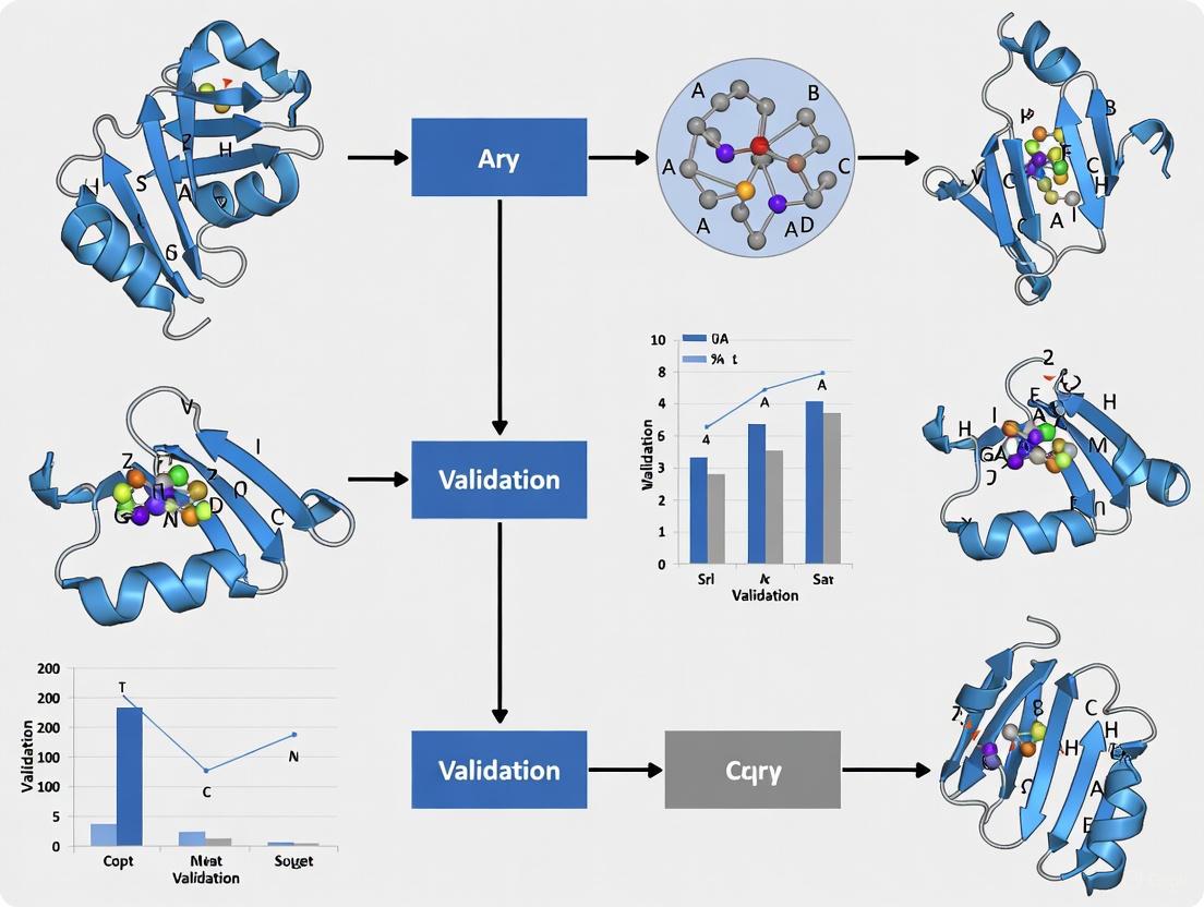
The following workflow illustrates a robust protocol for validating energy-minimized structures using molecular dynamics simulations:

This protocol implements a multistage approach that begins with energy minimization to remove steric clashes and unfavorable contacts, followed by gradual introduction of the time dimension through equilibration phases, ultimately leading to production MD simulations that sample the configurational space accessible at physiological conditions.

Experimental Validation of Simulated Structures

A critical challenge in molecular simulations lies in properly comparing simulated structures with experimental data. A specialized protocol has been developed "for comparing the structural properties of lipid bilayers determined by simulation with those determined by diffraction experiments, which makes it possible to test critically the ability of molecular dynamics simulations to reproduce experimental data" [5].

This model-independent method analyzes MD simulation data in the same manner as experimental data by determining structure factors and reconstructing transbilayer scattering-density profiles through Fourier transformation. When applied to dioleoylphosphatidylcholine (DOPC) bilayers, this approach revealed that "neither the GROMACS nor the CHARMM22/27 simulations reproduced experimental data within experimental error," with particularly strong disagreement in the widths of terminal methyl distributions [5]. This demonstrates that even MD simulations with current force fields may not fully capture experimental reality, highlighting the essential role of experimental validation.

Advanced Sampling Techniques for Complex Systems

For large or complex systems like supramolecular assemblages, enhanced sampling techniques become necessary. Recent research demonstrates innovative approaches where "the protein structure can be described at a mixed-resolution to perform atomistic modeling in the functional regions of the protein, and a lower-resolution modeling is applied in the remaining parts to reduce the computational cost" [6].

This methodology combines anisotropic network modeling (ANM) to generate plausible conformers, followed by docking calculations and all-atom MD simulations of truncated binding sites to estimate binding free energies. Application to triose phosphate isomerase (TIM) demonstrated that 100 ns MD simulations provided sufficient sampling to estimate binding affinities accurately, with comparable results between intact and truncated structures [6]. This approach offers a computationally efficient framework for validating minimized structures in biologically relevant contexts.

Essential Research Reagents and Computational Tools

The table below details key computational tools and methodologies referenced in the studies discussed, providing researchers with practical resources for implementing the protocols described:

Research Tool	Function/Purpose	Application Context
GROMACS	Molecular dynamics simulation package	Polymer interfacial studies [3], lipid bilayer validation [5]
OPLS-AA	All-atom force field parameters	Polymer-solvent interactions [3]
Steepest Descent	Energy minimization algorithm	Initial structure relaxation [2]
L-BFGS	Quasi-Newton minimization	Efficient localization of minima [2] [4]
Sella	Geometry optimization package	Transition state and minimum optimization [4]
geomeTRIC	Optimization with internal coordinates	Molecular structure optimization [4]
ANM	Anisotropic Network Model	Efficient conformational sampling [6]
MM-GBSA	Molecular Mechanics/Generalized Born Surface Area	Binding free energy calculations [6]

These tools represent the essential computational "reagents" required for implementing robust protocols that combine energy minimization with molecular dynamics validation. The selection of appropriate tools depends on system characteristics, with smaller systems benefiting from more exhaustive sampling methods, while larger systems may require mixed-resolution or enhanced sampling approaches to achieve sufficient conformational coverage within practical computational constraints.

Energy minimization remains an essential first step in molecular simulations, efficiently removing steric clashes and locating local energy minima. However, its fundamental limitations—particularly the missing time dimension and inability to escape local minima—make it insufficient as a standalone approach for predicting biologically relevant structures. The integration of EM with molecular dynamics simulations creates a powerful framework that combines the efficiency of local minimization with the physically realistic sampling provided by temporal evolution.

Validation against experimental data remains the ultimate test for any computational approach. The protocols discussed herein, particularly those that analyze MD trajectories using the same methods as experimental data [5], provide robust frameworks for assessing predictive accuracy. As force fields continue to improve and sampling methods become more efficient, the combination of EM and MD will increasingly enable researchers to bridge the gap between static molecular structures and dynamic biological function, ultimately accelerating drug discovery and materials design.

For researchers and drug development professionals, the practical implication is clear: energy-minimized structures should be viewed as starting points rather than final predictions. Subsequent molecular dynamics simulation and experimental validation are essential steps for developing reliable molecular models that accurately represent behavior under physiological conditions. This integrated approach moves computational research beyond the limitations of local minima and the timeless world of pure energy minimization into the dynamic realm of molecular reality.

Molecular dynamics (MD) simulations have become an indispensable tool in the computational molecular sciences, providing unparalleled insight into the atomistic motions and time-dependent behavior of biological systems. While static structures offer a snapshot of molecular architecture, they fail to capture the dynamic nature essential for function. MD simulations bridge this gap, serving as a powerful validation tool to probe the stability, flexibility, and realistic conformational landscapes of biomolecules. As the reliance on computationally predicted protein structures grows with advances in tools like AlphaFold2, the importance of MD for validating these models has increased correspondingly. This guide examines how MD simulations are applied to assess and refine molecular models, comparing various methodological approaches and their effectiveness across different protein systems and states.

Fundamental Validation Metrics in Molecular Dynamics

MD simulations generate terabytes of trajectory data, which researchers distill into quantitative metrics to assess structural stability, flexibility, and dynamic behavior. The most fundamental metrics provide insights into different aspects of protein dynamics and are routinely applied across diverse studies.

Table 1: Core Metrics for MD-Based Validation

Metric	Description	Interpretation	Application Example
Root Mean Square Deviation (RMSD)	Measures average displacement of atoms relative to a reference structure	Lower values indicate stable convergence; rising trends suggest structural drift	FtsZ tense conformation showed 2.7-3.1 Å RMSD with GDP, indicating instability [7]
Root Mean Square Fluctuation (RMSF)	Quantifies per-residue flexibility throughout simulation	Peaks indicate flexible regions; valleys represent structural constraints	T6 and T7 loops in SH3 domain showed higher flexibility in GTP-bound states [8] [7]
Radius of Gyration (Rg)	Measures structural compactness	Decreasing values suggest compaction; increases may indicate unfolding	Used to assess folding quality in benchmark datasets [9]
Essential Dynamics (PCA)	Identifies collective motions from covariance matrices	Large eigenvalues represent functionally relevant motions	Differentiated conformational dynamics in SH3 domain mutants [8]

These metrics enable researchers to move beyond qualitative assessment to quantitative validation of structural models. For instance, RMSD analysis of FtsZ proteins from Staphylococcus aureus and Bacillus subtilis revealed that relaxed conformations were stable (RMSD 1.2-1.6 Å) regardless of bound nucleotide, while tense conformations formed higher energetic states, particularly when bound to GDP (RMSD 2.7-3.1 Å) [7]. Such analyses validate whether a predicted or modeled structure maintains stability under simulation conditions or exhibits problematic flexibility.

MD for Validation of Specific Molecular Systems

Validation of De Novo Designed Proteins

MD simulations play a crucial role in validating computationally designed proteins, assessing whether designed structures maintain their intended conformations and possess dynamics compatible with their functional goals. Studies have revealed that designed proteins often exhibit exceptional stability, sometimes exceeding naturally occurring proteins [10]. Through MD analysis, researchers have identified structural bases for this stability, including optimized core packing, increased burial of hydrophobic surface area, and favorable arrangements of charged residues.

For example, MD simulations of the designed protein AYEdes demonstrated decreased RMSD and RMSF values, decreased solvent-accessible surface area, increased secondary structure retention, and more favorable contact networks compared to reference structures [10]. Similarly, analysis of successful versus unsuccessful digoxigenin-binding protein designs revealed that successful designs had more rigid cavity entrances, better-organized hydrophobic cores, smaller cavity volumes, and preorganized ligand-binding side chains [10].

Assessment of Intrinsically Disordered Proteins

Validating models of intrinsically disordered proteins presents unique challenges due to their inherent flexibility and lack of stable tertiary structure. MD simulations have been successfully integrated with experimental data from NMR spectroscopy and small-angle X-ray scattering to determine accurate atomic-resolution conformational ensembles of IDPs [11]. The maximum entropy reweighting procedure has emerged as a powerful approach, introducing minimal perturbation to computational models required to match experimental data.

Studies on IDPs including Aβ40, drkN SH3, ACTR, PaaA2, and α-synuclein have demonstrated that in favorable cases, where IDP ensembles obtained from different MD force fields show reasonable initial agreement with experimental data, reweighted ensembles converge to highly similar conformational distributions after reweighting [11]. This approach represents substantial progress toward force-field independent integrative structural biology of disordered proteins.

Refinement of Predicted Structures

MD serves as a crucial refinement tool for structures predicted through computational methods. A study on hepatitis C virus core protein demonstrated that MD simulations compactly folded protein structures predicted by various tools (AlphaFold2, Robetta, trRosetta, MOE, I-TASSER), resulting in theoretically accurate models [12]. The root mean square deviation of backbone atoms, root mean square fluctuation of Cα atoms, and radius of gyration effectively monitored structural changes and convergence during the refinement process [12].

Table 2: MD Applications Across Protein States

Protein State	Key MD Validation Approaches	Challenges	Notable Findings
Designed Proteins	Stability assessment (RMSD/RMSF), contact analysis, hydration analysis	Balancing stability with functional dynamics	Some designs show exceptional thermostability; successful designs preorganize functional sites [10]
Intrinsically Disordered Proteins	Maximum entropy reweighting with experimental data, ensemble comparison	Sparse experimental data, force field dependencies	Reweighted ensembles from different force fields can converge to similar distributions [11]
Predicted Structures	Post-prediction refinement, quality assessment via ERAT and phi-psi plots	Initial model quality, sampling limitations	MD refinement improves model quality scores and produces more reliable structural models [12]

Advanced Sampling and Machine Learning Approaches

Conventional MD simulations face limitations in sampling rare events due to temporal constraints. Enhanced sampling methods and machine learning approaches have emerged to address these challenges, providing more efficient exploration of conformational landscapes.

Generative and Committor-Guided Methods

The Gen-COMPAS framework represents a recent advancement, combining generative diffusion models with committor analysis to reconstruct transition pathways without predefined collective variables [13]. This approach generates physically realistic intermediates and uses committor-based filtering to identify transition states, enabling rapid convergence of transition-path ensembles within nanoseconds compared to traditional enhanced-sampling methods that require orders of magnitude more sampling [13].

Applied to systems ranging from miniproteins to ribose-binding proteins and mitochondrial carriers, Gen-COMPAS successfully retrieves committors, transition states, and free-energy landscapes efficiently, demonstrating the power of uniting machine learning with molecular dynamics for mechanistic insight [13].

Benchmarking and Weighted Ensemble Approaches

Standardized benchmarking has become increasingly important as MD methods diversify. A recent modular benchmarking framework systematically evaluates protein MD methods using weighted ensemble sampling based on progress coordinates derived from time-lagged independent component analysis [9]. This approach enables fast and efficient exploration of protein conformational space and supports both classical force fields and machine learning-based models.

The framework includes comprehensive evaluation of over 19 different metrics across diverse domains, applied to a dataset of nine proteins ranging from 10 to 224 residues that span various folding complexities and topologies [9]. Such standardized evaluation enables direct, reproducible comparisons across MD approaches, addressing a critical gap in the molecular simulation community.

Experimental Protocols and Workflows

Standard MD Validation Protocol

A typical MD-based validation protocol involves multiple stages of simulation and analysis. The process generally begins with system preparation, where the protein structure is solvated in water molecules with ions added to neutralize the system. Energy minimization removes steric clashes, followed by gradual heating and equilibration phases to stabilize temperature and density. Production simulation then proceeds, typically for tens to hundreds of nanoseconds, during which coordinates are saved for subsequent analysis [8] [7].

For the α-spectrin SH3 domain and its mutants, researchers performed 40 ns simulations using GROMACS with the GROMOS96 43a2 force field, explicit SPC water model, and particle mesh Ewald method for long-range electrostatics [8]. Conformational analysis employed a two-level approach combining self-organizing maps and hierarchical clustering to identify functionally relevant conformations and highlight differences in conformational dynamics [8].

Standard MD Validation Workflow

Integrative Validation with Experimental Data

For higher-accuracy validation, particularly with challenging systems like IDPs, integrative approaches combine MD with experimental data. The maximum entropy reweighting procedure represents one such methodology, determining accurate atomic-resolution conformational ensembles by integrating all-atom MD simulations with experimental data from NMR spectroscopy and SAXS [11].

This workflow involves running long-timescale MD simulations with different force fields, predicting experimental observables for each simulation frame using forward models, and then reweighting the ensembles to achieve optimal agreement with experimental data while maintaining maximum entropy [11]. The approach automatically balances restraints from different experimental datasets based on the desired effective ensemble size, producing statistically robust ensembles with minimal overfitting.

Integrative Validation Workflow

The Scientist's Toolkit: Essential Research Reagents and Solutions

Successful MD validation requires appropriate tools and methodologies. The table below outlines key computational "reagents" essential for effective MD-based validation studies.

Table 3: Essential Research Reagents for MD Validation

Tool Category	Specific Tools	Function	Application Notes
Simulation Engines	GROMACS, AMBER, OpenMM	Perform molecular dynamics calculations	GROMACS favored for speed; AMBER for force field variety; OpenMM for GPU acceleration [8] [9] [14]
Force Fields	CHARMM36m, a99SB-disp, GROMOS96	Define molecular interactions and potentials	CHARMM36m and a99SB-disp show strong performance for IDPs; choice depends on system [11]
Analysis Suites	MDTraj, MDAnalysis, GROMACS tools	Process trajectories and calculate metrics	MDTraj offers Python API; MDAnalysis provides comprehensive analysis suite [8] [9]
Enhanced Sampling	GaMD, Metadynamics, WE	Accelerate rare event sampling	GaMD valuable for glycosidic linkage transitions; WE effective for protein folding [14] [9]
Benchmarking	MDBenchmark, WESTPA	Assess simulation performance and sampling	MDBenchmark optimizes computing resource use; WESTPA implements weighted ensemble [15] [9]

Molecular dynamics simulations have evolved into sophisticated validation tools capable of probing the stability, flexibility, and conformational landscapes of biomolecules with atomic resolution. Through quantitative metrics like RMSD and RMSF, advanced sampling methods, and integration with experimental data, MD provides critical insights that complement static structural models. As computational protein design and prediction continue advancing, robust MD validation protocols will become increasingly essential for verifying structural models and ensuring their biological relevance. The continued development of standardized benchmarking frameworks and integrative methods promises to further enhance the reliability and applicability of MD as a validation tool across diverse biological systems.

In molecular dynamics (MD) research, validating the stability of minimized structures is a critical step for ensuring the reliability of computational models in drug development and structural biology. Stability metrics provide quantitative, time-dependent measures to assess whether a simulated molecular system has reached a physiologically relevant equilibrium or if it undergoes significant conformational changes. Among the most critical metrics are the Root-Mean-Square Deviation (RMSD), which measures the average atomic displacement of a structure relative to a reference, typically indicating global conformational stability; the Radius of Gyration (Rg), which quantifies the compactness and overall dimensions of a molecular structure; and Energy Fluctuations, which reflect the thermodynamic stability of the system through the conservation of potential and kinetic energy. These metrics are indispensable for benchmarking the performance of different modeling algorithms, such as AlphaFold, PEP-FOLD, and homology modeling, and for verifying that a minimized structure represents a stable, native-like conformation rather than a transient or unstable state [16]. This guide objectively compares these core stability metrics, detailing their experimental protocols, interpretation, and application in contemporary research.

Comparative Analysis of Key Stability Metrics

The table below provides a structured comparison of the three primary stability metrics, detailing their core functions, analytical focus, and interpretation guidelines.

Table 1: Comparative Analysis of Key Structural Stability Metrics

Metric	Core Function & Analytical Focus	Data Interpretation Guidelines	Representative Values from Recent Studies
Root-Mean-Square Deviation (RMSD)	Measures global structural drift by calculating the average distance between atoms after optimal alignment to a reference structure [17].	Low, stable RMSD: Conformational stability is achieved [18].Sudden RMSD jumps: Possible conformation change or unfolding event.Gradual, continuous rise: System may not be equilibrated.	Protein backbone: ~1.5-3.0 Å (stable complex) [18] [17].Ligand atoms: < 1.0 Å (stable binding) [17].
Radius of Gyration (Rg)	Measures structural compactness and overall shape, calculated as the mass-weighted root mean square distance of atoms from the structure's center of mass [19].	Decreasing Rg: System is collapsing or becoming more compact.Stable Rg: Maintains a consistent fold and packing.Increasing Rg: Structure is expanding or loosening, potentially unfolding.	Folded proteins: ( R_g(N) \propto N^{\nu} ), with ( \nu \sim 1/3 ) for a compact, globular state [19].
Energy Fluctuations	Assesses thermodynamic stability by monitoring the conservation of total energy in the system (NVE ensemble) or the stability of potential energy over time (NVT/NPT ensembles) [20].	Stable total energy (NVE): Validates the integrity of the simulation and energy conservation.Stable potential energy: Indicates the system is in a state of equilibrium. Large drifts suggest instability.	-

Experimental Protocols for Metric Analysis

A robust MD protocol is essential for obtaining reliable and reproducible metric data. The following workflow and detailed methodology are synthesized from current research practices.

System Preparation and Simulation

• Initial Structure Minimization: Begin with a modeled or experimentally derived structure (e.g., from PDB). Use steepest descent or conjugate gradient algorithms to remove steric clashes and bad contacts, ensuring the structure is at a local energy minimum [16].
• Solvation and Ionization: Place the molecule in a physiologically relevant solvent box (e.g., TIP3P water model). Add ions to neutralize the system's charge and achieve a desired ionic concentration, mimicking a biological environment.
• Equilibration Phases:
  • NVT Ensemble: Equilibrate the system with a constant Number of particles, Volume, and Temperature (typically 300 K using a thermostat like Nosé-Hoover) for 100-500 ps. This allows the system to reach the target temperature.
  • NPT Ensemble: Further equilibrate with a constant Number of particles, Pressure (1 bar using a barostat like Parrinello-Rahman), and Temperature for 100-500 ps. This allows the solvent density to adjust correctly and the box size to stabilize.
• Production MD Run: Perform an extended simulation using an integrator like LINCS under the desired ensemble (NPT for stability studies). The duration must be sufficient to capture relevant biological dynamics; for protein folding or peptide stability, this can range from 100 ns to several microseconds [16] [18]. A 100 ns simulation is a common benchmark for initial stability validation [16].

Trajectory Analysis and Metric Calculation

• Trajectory Processing: Before analysis, ensure trajectories are correctly aligned (e.g., to the protein backbone) to remove global rotation and translation.
• RMSD Calculation: The RMSD is calculated as: ( \text{RMSD}(t) = \sqrt{ \frac{1}{N} \sum{i=1}^{N} \lvert \vec{r}i(t) - \vec{r}i^{\text{ref}} \rvert^2 } ) where ( \vec{r}i(t) ) is the position of atom ( i ) at time ( t ), ( \vec{r}_i^{\text{ref}} ) is its position in the reference structure (often the minimized or starting structure), and ( N ) is the number of atoms [21] [18]. This is typically calculated for backbone atoms (C, Cα, N) to assess the core structural stability.
• Radius of Gyration (Rg) Calculation: The Rg is calculated as: ( Rg = \sqrt{ \frac{1}{M} \sum{i=1}^{N} mi \lvert \vec{r}i - \vec{r}{\text{com}} \rvert^2 } ) where ( mi ) is the mass of atom ( i ), ( M ) is the total mass, ( \vec{r}i ) is the position of atom ( i ), and ( \vec{r}{\text{com}} ) is the center of mass of the molecule [19]. This can be calculated for the entire molecule or specific subchains to analyze internal packing.
• Energy Fluctuation Analysis: Monitor the total energy (in NVE simulations) and the potential energy (in NPT/NVT simulations) over time. The system is considered thermodynamically stable if these values fluctuate steadily around a constant mean without significant drifts [20].

The Scientist's Toolkit: Essential Research Reagents and Software

The table below lists key computational tools and their functions, as utilized in the cited experimental studies.

Table 2: Essential Research Reagents & Software Solutions

Tool Name	Primary Function	Application Example
GROMACS	A versatile package for performing MD simulations, including trajectory analysis [22].	Used for all-atom MD simulations to predict crystal structures of bowl-shaped π-conjugated molecules and analyze their energy landscapes [22].
Desmond	A high-performance MD simulator designed for biomolecular systems [18].	Employed for 500 ns simulations of carbonic anhydrase XII with inhibitors to study binding stability and conformational changes [18].
LAMMPS	A classical molecular dynamics code for modeling materials at the atomic scale [23].	Applied to study the stratification behavior of methane-hydrogen mixtures under different gravitational fields [23].
AutoDock Vina / InstaDock	Molecular docking and virtual screening tools for predicting ligand binding poses and affinities [24].	Used for high-throughput virtual screening to identify natural inhibitors targeting the αβIII-tubulin isotype [24].
AlphaFold / PEP-FOLD	Algorithms for predicting protein and peptide structures from amino acid sequences [16].	Compared for their efficacy in modeling short, unstable antimicrobial peptides (AMPs) [16].

Integrated Interpretation: A Case Study in Cancer Drug Discovery

The power of these integrated metrics is exemplified in a 2025 study investigating carbonic anhydrase XII (CA XII) inhibitors for cancer therapy. Researchers combined RMSD, Rg, and energy analyses to validate the stability of a novel inhibitor (V35) bound to the target protein. Over a 500 ns simulation, the protein-ligand complex exhibited a stable backbone RMSD of around 1.5-2.0 Å, indicating minimal global structural drift. The Rg value remained constant, confirming that the protein maintained its compact, folded conformation without unfolding or significant expansion. Concurrently, stable potential energy and favorable MM/GBSA binding free energy calculations (-44.17 kcal/mol for V35) confirmed the thermodynamic stability of the complex. This multi-metric validation provided high confidence that the minimized structure of the V35-CA XII complex was stable and reliable for further analysis and design, underscoring the compound's potential as a lead therapeutic candidate [18].

RMSD, Rg, and energy fluctuations are non-redundant, complementary metrics that form the cornerstone of structural validation in molecular dynamics. While RMSD provides a macro-level view of conformational stability, and Rg offers insight into structural compactness, energy fluctuations underpin the thermodynamic validity of the simulation. As demonstrated in cutting-edge research, from validating AI-predicted peptide structures to designing isoform-selective drugs, the triangulation of data from these metrics is essential for benchmarking computational models and making confident decisions in rational drug design. Researchers are advised to always apply these metrics in concert, as their integrated story provides a far more reliable assessment of structural stability than any single metric alone.

Accurate prediction of short peptide structures represents a significant challenge in computational biology, with direct implications for therapeutic development, particularly for antimicrobial peptides (AMPs) and other bioactive sequences [16]. Short peptides are often highly flexible and can adopt numerous conformations in solution, making them difficult to model with traditional algorithms trained primarily on globular proteins [25]. This case study examines how Molecular Dynamics (MD) simulations have emerged as a crucial validation tool for assessing the performance of structure prediction algorithms, with a specific focus on revealing the complementary strengths of AlphaFold and PEP-FOLD when applied to short peptides.

The study is framed within a broader thesis on validating minimized structures with molecular dynamics research, demonstrating how computational validation pipelines can guide researchers in selecting appropriate tools based on peptide characteristics. By integrating MD simulations as a benchmark, researchers can move beyond static structural snapshots to evaluate conformational stability under physiologically relevant conditions [16] [25].

Methodology: Comparative Modeling and MD Validation Framework

Peptide Selection and Characterization

The foundational study selected 10 putative antimicrobial peptides randomly derived from the human gut metagenome, with lengths falling within the typical AMP range (12-50 amino acids) [16]. Prior to structure prediction, researchers conducted comprehensive physicochemical characterization using the ExPASy-ProtParam tool to calculate key properties including isoelectric point (pI), aromaticity, grand average of hydropathicity (GRAVY), and instability index [16]. This initial profiling enabled subsequent correlation between peptide properties and algorithmic performance.

Disordered regions were predicted using the RaptorX server, which employs a Deep Convolutional Neural Fields (DeepCNF) model to forecast structural disorder, secondary structure, and solvent accessibility [16]. This step was particularly important for interpreting MD results, as disordered regions typically exhibit higher flexibility during simulations.

Structure Prediction Algorithms

Four distinct modeling approaches were selected to represent the spectrum of current methodologies [16]:

• AlphaFold: Deep learning-based approach utilizing evolutionary constraints and attention mechanisms
• PEP-FOLD3: De novo fragment-assembly method based on structural alphabet letters
• Threading: Template-based approach leveraging known protein folds
• Homology Modeling: Comparative modeling using MODELLER with related structures

This strategic selection enabled direct comparison between template-based, de novo, and deep learning methods, providing insights into their respective strengths and limitations for short peptide modeling.

Validation Metrics and MD Protocol

The validation pipeline incorporated multiple complementary approaches [16]:

• Ramachandran plot analysis to assess backbone dihedral angle quality
• VADAR for comprehensive structural validation
• Molecular Dynamics simulations for stability assessment

For MD simulations, researchers performed 40 independent simulations (4 structures × 10 peptides), each with 100 ns duration using GROMACS software [16]. The simulation protocol included system solvation in TIP3P water models, application of the AMBER force field, and implementation of periodic boundary conditions to mimic physiological environments [26] [27]. Trajectory analysis focused on stability metrics, including RMSD, RMSF, and intramolecular interactions.

Results: MD Reveals Algorithm-Specific Strengths

Performance Across Peptide Classes

Molecular dynamics simulations demonstrated that algorithmic performance was strongly influenced by peptide physicochemical properties, particularly hydrophobicity [16]. The stability of predicted structures during MD simulations revealed complementary strengths between the different approaches.

Table 1: Algorithm Performance Based on Peptide Properties

Peptide Characteristic	Optimal Algorithm(s)	Key Observations from MD Simulations
High hydrophobicity	AlphaFold & Threading	Structures maintained compact folds with stable hydrophobic cores
High hydrophilicity	PEP-FOLD & Homology Modeling	Better solvation and stable hydrogen bonding networks
Mixed secondary structures	PEP-FOLD	More accurate β-turn and loop predictions
α-helical bias	AlphaFold	High accuracy in helix geometry and packing
Disordered regions	PEP-FOLD	More realistic flexibility in unstructured regions

Quantitative Stability Metrics from MD

The root mean square deviation (RMSD) analysis throughout 100 ns simulations provided quantitative measures of structural stability. PEP-FOLD generated structures that generally exhibited lower RMSD fluctuations after equilibration, indicating greater conformational stability under simulation conditions [16]. AlphaFold predictions, while often initially more compact, in some cases showed higher RMSD values during simulations, suggesting structural adjustments toward more stable conformations [25].

Radius of gyration (Rg) measurements revealed that AlphaFold frequently produced more compact starting structures, while PEP-FOLD structures maintained more consistent compactness throughout simulations [16]. This observation suggests differences in how these algorithms handle the balance between intramolecular interactions and solvation effects.

Comparative Accuracy Assessment

Table 2: Algorithm Performance Benchmarking for Short Peptides

Algorithm	Approach	Strength Areas	MD Validation Insights	Key Limitations
AlphaFold	Deep learning	α-helical peptides, compact folds [16] [28]	pLDDT scores don't always correlate with MD stability [25] [28]	Challenged by mixed secondary structures, orphan proteins [29] [25]
PEP-FOLD	De novo fragment assembly	Hydrophilic peptides, stable dynamics [16] [30]	Maintains structural stability during MD simulations [16]	Limited to 9-36 amino acids; lower Z-scores [30] [31]
Threading	Template-based	Hydrophobic peptides [16]	Complementary to AlphaFold for certain peptide classes [16]	Template dependency limits novel fold prediction
Homology Modeling	Comparative modeling	Hydrophilic peptides [16]	Moderate performance across peptide types [16]	Requires suitable templates

Recent benchmarking studies involving 588 peptide structures confirmed that while AlphaFold predicts α-helical, β-hairpin, and disulfide-rich peptides with high accuracy, its pLDDT confidence metric does not always correlate with lowest RMSD to experimental structures [28]. This highlights the critical importance of MD validation for identifying the most accurate predicted conformations.

Integrated Workflow for Peptide Structure Prediction

The following workflow diagram illustrates the integrated approach for peptide structure prediction and validation revealed by the case study:

The Scientist's Toolkit: Essential Research Reagents

Table 3: Computational Tools for Peptide Structure Prediction and Validation

Tool Category	Specific Tools	Function	Application Notes
Structure Prediction	AlphaFold 2/3, PEP-FOLD 4, I-TASSER 5.1	Generate 3D structural models from sequence	AlphaFold excels for single-chain proteins; PEP-FOLD for de novo peptide folding [16] [31]
MD Simulation	GROMACS, AMBER	Simulate dynamic behavior and validate stability	GROMACS recommended for efficiency with peptide systems [16] [26]
Structure Validation	VADAR, PROCHECK, MolProbity	Assess stereochemical quality	Ramachandran analysis critical for backbone validation [16]
Physicochemical Analysis	ExPASy-ProtParam, Prot-pi	Calculate charge, hydropathicity, instability index	Essential for correlating properties with algorithm performance [16]
Disorder Prediction	RaptorX, DISOPRED3	Identify intrinsically disordered regions	Important for interpreting MD fluctuations [16]

Discussion: Implications for Rational Peptide Design

The integration of MD simulations as a validation tool has fundamentally transformed our understanding of computational peptide modeling. Rather than seeking a universal "best" algorithm, researchers can now adopt a property-informed selection strategy where peptide characteristics guide tool selection [16]. This approach recognizes that the biophysical properties of peptides significantly influence algorithmic performance.

The finding that AlphaFold and PEP-FOLD display complementary strengths based on peptide hydrophobicity has practical implications for drug development pipelines [16]. For hydrophobic peptides (common in membrane-active AMPs), an AlphaFold-first approach with MD validation may be optimal. For hydrophilic or mixed-charge peptides, PEP-FOLD may produce more stable structures. This paradigm shift from universal to context-dependent algorithm selection represents a significant advancement in computational structural biology.

Furthermore, the observation that AlphaFold's pLDDT scores do not consistently correlate with MD stability for short peptides highlights the necessity of dynamical validation [25] [28]. This suggests that confidence metrics from static prediction algorithms should be interpreted cautiously, and MD simulations provide essential complementary information about conformational stability under near-physiological conditions.

This case study demonstrates that Molecular Dynamics simulations serve as an essential tool for validating and benchmarking structure prediction algorithms for short peptides. Through comprehensive MD validation, researchers have discovered that AlphaFold and PEP-FOLD exhibit complementary strengths that correlate with peptide physicochemical properties.

The key insight is that algorithm performance is context-dependent – AlphaFold excels with hydrophobic peptides and compact folds, while PEP-FOLD generates more stable structures for hydrophilic peptides and maintains better dynamical stability during simulations. These findings support the development of integrated prediction pipelines where multiple algorithms are applied in parallel, with MD simulations serving as the final arbiter of structural quality.

For researchers pursuing rational design of therapeutic peptides, these findings suggest a strategic approach: (1) characterize peptide physicochemical properties, (2) select algorithms based on these properties, (3) generate multiple structural models, and (4) employ MD simulations to identify the most stable conformations. This property-informed modeling strategy, validated by molecular dynamics, will accelerate the development of peptide-based therapeutics by providing more reliable structural models for interaction analysis and functional studies.

Executing Validation: A Step-by-Step MD Protocol for Robust Structure Assessment

In molecular dynamics (MD) research, the initial, energy-minimized structure of a biomolecule represents only a starting point. Validating this structure requires simulating its behavior in a realistic environment, a process central to bridging the gap between static structural data and biological function [32] [33]. The methods used to solvate the molecule, place ions, and define the surrounding medium directly determine the simulation's physical accuracy and its relevance to experimental observations. For drug discovery professionals, a correctly built system is indispensable for reliable investigations into mechanisms of action, stability, and molecular interactions [33] [34].

This guide objectively compares the predominant approaches for constructing these simulation environments: explicit solvent models, which simulate every water molecule and ion, and implicit solvent models, which represent the solvent as a dielectric continuum. We will evaluate their performance in the context of validating minimized structures, supported by experimental data and detailed protocols.

Core Concepts and Research Reagents

Before comparing methodologies, it is essential to understand the key components and tools that constitute the "simulation environment." The table below details the essential research reagents and software solutions used in this field.

Table 1: Key Research Reagents and Software Solutions for MD Simulations

Item/Software	Type/Provider	Primary Function in Simulation Setup
TP3P, SPC/E Water Models	Explicit Solvent Model	Provides an atomic-level representation of water molecules, capturing granular solvent effects and viscosity [35].
Generalized Born (GB) Model	Implicit Solvent Model	Approximates solvation free energy as a sum of polar and nonpolar terms, significantly speeding up calculations by replacing explicit water [32].
Molecular Operating Environment (MOE)	Software / Chemical Computing Group	An all-in-one platform for molecular modeling, cheminformatics, and structure-based drug design, useful for initial system building [36].
AMBER	MD Package	A widely used MD software suite that provides tools for system building (e.g., tleap), explicit and implicit solvent simulation, and advanced analysis [32].
GROMACS	MD Package	A high-performance MD software known for its speed, often optimized for GPU computing, used for simulating biomolecules in explicit solvent [34] [37].
Schrödinger Suite	Software / Schrödinger	A comprehensive platform that integrates quantum chemical methods, machine learning, and MD for molecular modeling and free energy calculations [36].

Methodological Comparison: Explicit vs. Implicit Solvation

The choice between explicit and implicit solvent is a fundamental decision that trades off computational cost for physical detail. The following workflow outlines the standard protocol for building a simulation system, highlighting steps that differ between the two approaches.

Diagram 1: Workflow for Building an MD Simulation System.

The table below provides a direct performance comparison of these two methods, illustrating the core trade-offs.

Table 2: Performance Comparison of Explicit vs. Implicit Solvent Models

Feature	Explicit Solvent (e.g., TIP3P)	Implicit Solvent (e.g., GB)
Physical Realism	High. Captures specific water structure, hydrogen bonding, and diffusion [32] [35].	Low. Lacks explicit water molecules, missing atomic-level solvent details [32].
Computational Cost	Very High. Can require simulating 10x more particles; dramatically slower [35].	Low. Much faster, allowing for longer timescale simulations [32].
Ion Effects	Explicitly models discrete ions and their dynamics [32] [38].	Models ionic strength as a continuum, missing specific ion interactions [38].
Salt Bridge Stability	Accurate. Can show solvent-separated states and realistic dynamics [38].	Often over-stabilized. Contact pairs are typically too stable compared to explicit solvent [38].
Ideal Use Case	Final validation of dynamics, studying specific solvent-ion interactions, and parameterizing coarse-grained models [32] [38].	Initial stability checks, rapid sampling, and large-scale conformational changes [32].

Experimental Protocols and Validation Data

Detailed Protocol: Explicit Solvent System Setup

The following protocol, adapted for a system like an siRNA duplex, is typical for setting up an explicit solvent simulation using the AMBER package [32].

• Force Field and Topology Preparation: Load the initial PDB file into the tleap module. Apply a nucleic acid force field (e.g., ff14SB or OL3). This step assigns parameters for bonded and non-bonded interactions to every atom.
• Solvation in Explicit Water: The solute is immersed in a predefined box of explicit water molecules, such as TIP3P. A common command is solvateBox <molecule> TIP3PBOX 12.0, which places the solute in a box with a 12.0 Å buffer of water.
• Ion Placement: Ions are added to neutralize the system's net charge and to achieve a physiologically relevant ionic concentration (e.g., 0.15 M NaCl). In tleap, the command addIons2 <molecule> Na+ 0 adds sodium ions until the system charge is neutralized. Further ions can be added to match the desired concentration.
• System Equilibration: The fully solvated system undergoes a multi-stage energy minimization and equilibration process. This involves:
  • Minimization: Relaxing the solvent and ions around the fixed solute to remove steric clashes.
  • Heating: Gradually increasing the system temperature to the target (e.g., 300 K) under positional restraints on the solute.
  • Density Equilibration: A short simulation in the NPT ensemble (constant Number of particles, Pressure, and Temperature) to allow the solvent density to reach the correct value.
  • Unrestrained Equilibration: A final equilibration run with all restraints removed to ensure the system is stable before production dynamics.

Experimental Validation: Linking Simulation to Physicochemical Properties

The ultimate test of a properly built and validated system is its ability to predict or correlate with experimental data. A compelling example comes from research that uses MD simulations to predict a key pharmaceutical property: aqueous solubility.

Experimental Methodology [34]:

• A dataset of 211 diverse drug molecules was compiled with experimental aqueous solubility (logS) data.
• Each compound underwent MD simulation in explicit water (using GROMACS with the GROMOS 54a7 force field) to extract dynamic properties.
• Key MD-derived properties were calculated from the trajectories, including:
  • Solvent Accessible Surface Area (SASA)
  • Coulombic and Lennard-Jones (LJ) interaction energies between the solute and water.
  • Estimated Solvation Free Energy (DGSolv)
• These properties, along with the experimental octanol-water partition coefficient (logP), were used as features in machine learning models to predict solubility.

Results and Performance Data: The MD-derived properties demonstrated high predictive power. The Gradient Boosting machine learning algorithm achieved a predictive R² of 0.87 and a root mean square error (RMSE) of 0.537 for logS on a test set of compounds [34]. This performance is comparable to models based solely on chemical structure, confirming that simulations in a properly built explicit solvent environment can capture the essential molecular interactions governing solubility.

Table 3: Key MD-Derived Properties for Predicting Aqueous Solubility [34]

Property	Description	Influence on Solubility
logP	Octanol-water partition coefficient (experimental).	Well-established negative correlation; higher logP generally means lower solubility.
SASA	Solvent Accessible Surface Area.	Measures the compound's surface exposed to solvent; larger SASA often correlates with higher solubility.
Coulombic_t	Coulombic interaction energy over time.	Captures the strength of polar interactions with water; stronger favorable interactions increase solubility.
LJ	Lennard-Jones interaction energy.	Represents van der Waals dispersion forces with water; favorable interactions promote solubility.
DGSolv	Estimated Solvation Free Energy.	The overall free energy change of solvation; a more negative value favors dissolution.

Selecting the right simulation environment is not a one-size-fits-all decision but a strategic choice based on the research question. Explicit solvent methods remain the gold standard for final validation studies, providing the detail necessary to compare directly with biophysical experiments and to interrogate specific solvent-mediated interactions. In contrast, implicit solvent models offer a powerful tool for high-throughput screening and studying events over longer timescales where computational cost is prohibitive.

The validation of a minimized structure is complete only when its dynamic behavior in a realistic environment aligns with experimental evidence. As demonstrated by the successful prediction of drug solubility, a rigorously built simulation system is the critical link that transforms a static, minimized model into a dynamic, biologically relevant entity, thereby solidifying the role of MD as a cornerstone of modern molecular research and drug development.

Accurate force field parameters, potential energy functions, and receptor-ligand models are indispensable for modeling the solvation and binding of drug-like molecules to biological receptors [39]. In the context of validating minimized structures with molecular dynamics (MD) research, the selection of an appropriate force field fundamentally determines the reliability and predictive power of the simulation outcomes. The rapidly expanding chemical space of medicinally relevant scaffolds demands that these mathematical models exhibit exceptional transferability across diverse molecular systems. Among the most widely utilized frameworks in biomolecular simulations are CHARMM (Chemistry at HARvard Macromolecular Mechanics), AMBER (Assisted Model Building with Energy Refinement), and their generalized counterparts for small molecules—CGenFF and GAFF [39] [40]. This guide provides an objective comparison of these force fields, drawing upon experimental and simulation data to inform researchers, scientists, and drug development professionals in selecting the optimal model for their specific molecular systems and research objectives.

Historical Context and Design Philosophies

The CHARMM and AMBER force fields emerged from distinct developmental pathways with different philosophical underpinnings. CHARMM was originally developed for simulations of proteins and nucleic acids, focusing on accurate description of structures and non-bonded energies [40]. AMBER shares similar biomolecular targets but employs a different approach to parameterization, where the use of RESP (Restrained Electrostatic Potential) charges is intended to reduce the need for extensive torsional potentials compared to models with empirical charge derivation [40]. The fundamental divergence lies in their treatment of electrostatic interactions, which profoundly impacts their performance across various chemical environments.

The need to simulate drug-like small molecules necessitated the development of generalized force fields compatible with these biomolecular frameworks. The CHARMM General Force Field (CGenFF) extended the CHARMM biomolecular force field to small drug-like molecules, allowing parameterization of arbitrary compounds to model interactions with biomolecular receptors in a manner consistent with the CHARMM force field [39]. Similarly, the General AMBER Force Field (GAFF) was developed to extend the application of the AMBER biomolecular force field to small drug-like molecules [39]. These generalized force fields employ different parameterization strategies rooted in their respective philosophical foundations.

Fundamental Differences in Parameterization Approaches

Electrostatic Treatment: CGenFF assigns charges expected to most accurately represent the Coulombic interaction of an atom with a proximal TIP3 water molecule if evaluated in the gas phase using HF/6-31G(d) level quantum mechanical (QM) calculations [39]. This approach arguably captures the polarization effects of the condensed phase more explicitly. In contrast, GAFF uses the AM1-BCC charge model designed to accurately reproduce the electrostatic surface potential (ESP) around a molecule, also evaluated in the gas phase using HF/6-31G* level of QM theory [39]. GAFF's methodology leverages the overestimated gas-phase dipole moment under the presumption that condensed phase polarization effects are fortuitously present.

Training Data and Validation: Both CGenFF and GAFF are trained on large, chemically diverse collections of model compounds that presumably contain atom-types and connectivities representing vast spaces of medicinally relevant compounds [39]. However, their validation against experimental data reveals differential performance across various molecular systems. CGenFF's parameterization emphasizes consistency with the CHARMM biomolecular force field, while GAFF prioritizes broad coverage of organic chemical space with automated parameterization capabilities.

Table 1: Fundamental Characteristics of Generalized Force Fields

Feature	CGenFF	GAFF
Charge Model	HF/6-31G(d) Coulombic interaction with TIP3P water	AM1-BCC fitting to electrostatic surface potential
Biomolecular Compatibility	CHARMM	AMBER
Chemical Coverage	Drug-like small molecules	Organic and pharmaceutical molecules
Element Coverage	H, C, N, O, S, P, halogens	H, C, N, O, S, P, halogens
Automation Level	Moderate	High
Primary Strength	Condensed phase polarization	Gas phase electrostatic accuracy

Performance Comparison: Quantitative Assessment Across Molecular Systems

Hydration Free Energy Predictions

Hydration free energy (HFE) represents a crucial property in drug design, measuring a compound's affinity for water and influencing binding affinity. A comprehensive analysis of over 600 molecules from the FreeSolv dataset revealed that both CGenFF and GAFF demonstrate comparable overall accuracy in predicting absolute HFEs [39]. However, significant differences emerge at the level of specific functional groups, highlighting specialized strengths and limitations for particular chemical contexts.

Functional Group-Specific Performance: Molecules containing nitro-groups show divergent behavior—CGenFF over-solubilizes while GAFF under-solubilizes them in aqueous medium [39]. Amine-containing compounds are systematically under-solubilized, with this effect more pronounced in CGenFF than in GAFF [39]. Conversely, carboxyl groups are over-solubilized to a greater extent in GAFF than in CGenFF [39]. These systematic errors provide critical guidance for researchers studying compounds with these specific functional motifs, suggesting potential corrective strategies or alternative force field selection based on molecular composition.

Thermodynamic Property Reproduction

Evaluation of force field performance for bio-relevant compounds like furfural, 2-methylfuran, 2,5-dimethylfuran, and 5-hydroxymethylfurfural reveals nuanced differences in thermodynamic property prediction [41]. In assessments of liquid density and vapor-liquid equilibria, different force fields demonstrate variable agreement with experimental data, with no single force field universally superior across all compounds and properties.

Liquid Density Predictions: For furfural, GAFF and CHARMM27 overestimate density across temperatures, while OPLS-AA shows better agreement with experimental data [41]. Similar compound-specific performance variations emerge for 2-methylfuran and 2,5-dimethylfuran (DMF), where different force fields show alternating superiority in predicting temperature-dependent density trends [41]. These findings underscore the importance of context-dependent force field selection, particularly for thermodynamic studies of biofuels and biomass-derived compounds.

Cross-Solvation Free Energy Accuracy

A systematic evaluation of nine condensed-phase force fields against experimental cross-solvation free energies provides a robust assessment of their relative accuracies [42]. This analysis considered a matrix of cross-solvation free energies for 25 small molecules representative of alkanes, chloroalkanes, ethers, ketones, esters, alcohols, amines, and amides, offering comprehensive insights into force field performance across diverse chemical environments.

Table 2: Force Field Performance Metrics for Cross-Solvation Free Energies

Force Field	Correlation Coefficient	RMSE (kJ mol⁻¹)	Average Error (kJ mol⁻¹)
GROMOS-2016H66	0.88	2.9	-0.2
OPLS-AA	0.87	2.9	+0.2
OPLS-LBCC	0.86	3.3	+0.3
AMBER-GAFF2	0.84	3.3	-0.3
AMBER-GAFF	0.83	3.6	-0.6
OpenFF	0.82	3.6	-1.5
GROMOS-54A7	0.81	4.0	+1.0
CHARMM-CGenFF	0.80	4.2	-0.3
GROMOS-ATB	0.76	4.8	-0.1

The data reveals that CHARMM-CGenFF shows moderate performance with a correlation coefficient of 0.80 and RMSE of 4.2 kJ mol⁻¹, while GAFF and GAFF2 demonstrate improved accuracy with RMSE values of 3.6 and 3.3 kJ mol⁻¹, respectively [42]. These differences, while statistically significant, are distributed heterogeneously across compound classes, emphasizing the chemical context-dependence of force field performance.

Binding Affinity Prediction: Critical Applications in Drug Discovery

Protein-Ligand Binding Affinity Calculations

Predicting binding affinity of ligands to protein targets represents a cornerstone application in computer-aided drug design. Alchemical relative binding free energy (ΔΔG) calculations have demonstrated remarkable accuracy in this domain, with both CHARMM and AMBER/GAFF achieving performance comparable to commercial implementations like Schrödinger's FEP+ [43]. A large-scale study encompassing 482 perturbations from 13 different protein-ligand datasets reported an average unsigned error (AUE) of 3.64 ± 0.14 kJ mol⁻¹ for combined AMBER and CHARMM force fields, effectively equivalent to FEP+'s AUE of 3.66 ± 0.14 kJ mol⁻¹ [43].

Consensus Approaches: Combining results from multiple force fields through simple averaging or weighted schemes can enhance prediction accuracy, potentially mitigating individual force field biases [43]. This strategy proves particularly valuable in lead optimization stages where reliable relative binding affinities guide medicinal chemistry efforts.

Membrane Protein Applications

The application of ΔΔG calculations to membrane proteins like G protein-coupled receptors (GPCRs) introduces additional complexities due to heterogeneous lipid environments, buried water molecules, and intricate system setup [44]. Recent research demonstrates successful application of both AMBER-TI and AToM-OpenMM with GAFF parameters for predicting binding affinities of ligands to GPCRs, showing good agreement with experimental data [44]. This expansion into membrane protein systems highlights the continuing evolution of these force fields for pharmaceutically relevant targets beyond soluble proteins.

Experimental Protocols and Methodologies

Hydration Free Energy Calculation Protocol

The calculation of hydration free energies follows well-established alchemical pathways implemented in MD packages like CHARMM [39]. The fundamental approach involves:

Thermodynamic Cycle: HFE is computed as ΔGhydr = ΔGvac - ΔGsolvent, where ΔGvac and ΔGsolvent represent the free energy of turning off solute interactions in vacuo and in aqueous medium, respectively [39]. This corresponds to the change in standard chemical potential as a solute transfers from gas phase to aqueous phase at equilibrium.

Alchemical Transformation: A hybrid Hamiltonian H(λ) = λH₀ + (1-λ)H₁ connects the endpoint states (fully interacting and non-interacting solute) through a coupling parameter λ ∈ [0,1] [39]. The solute is progressively annihilated from its environment using multiple simulation blocks for water molecules, dummy particles, and the solute itself.

System Setup: The simulation system consists of the solute molecule in a cubic box of explicit water (TIP3P model) with periodic boundary conditions, allowing at least 14Å between the solute and box edges [39]. Non-bonded interactions are typically truncated at 12Å, with free energy calculations performed using methods like MBAR, BAR, or TI.

Figure 1: Hydration Free Energy Calculation Workflow

Relative Binding Free Energy Protocol

Relative binding free energy calculations follow a dual transformation approach in complex and solvent environments [44] [43]:

System Preparation: Protein structures are prepared using tools like CHARMM-GUI Membrane Builder for membrane proteins or standard solvation for soluble proteins [44]. Ligands are parameterized using GAFF or CGenFF with charges calculated via AM1-BCC or RESP approaches.

Transformation Setup: The structural differences between ligand pairs are identified, and hybrid topologies are generated for alchemical transitions [43]. For each transformation, both electrostatic and van der Waals interactions are simultaneously scaled using softcore potentials to avoid singularities.

λ Scheduling: Multiple intermediate λ states (typically 12-16 windows) connect the physical end states [44]. Common λ values include 0.0, 0.0479, 0.1151, 0.2063, 0.3161, 0.4374, 0.5626, 0.6839, 0.7937, 0.8850, 0.9521, and 1.0, strategically distributed to ensure sufficient overlap between adjacent states.

Simulation and Analysis: Equilibration is performed at each λ window followed by production simulations. Free energy differences are computed via thermodynamic integration or free energy perturbation, with statistical precision enhanced through independent replicates [44].

Figure 2: Relative Binding Free Energy Calculation Workflow

Table 3: Computational Tools for Force Field Applications

Tool Name	Function	Compatibility
CHARMM/OpenMM	GPU-accelerated MD simulations with alchemical free energy methods	CHARMM/CGenFF
pmx	Hybrid topology generation for alchemical calculations with GROMACS	AMBER/CHARMM
CHARMM-GUI	Membrane protein system preparation	CHARMM/CGenFF
ANTECHAMBER	Automatic parameterization of organic molecules	AMBER/GAFF
pyCHARMM	Python framework embedding CHARMM's functionality	CHARMM/CGenFF
AMBER-TI	Thermodynamic integration implementation	AMBER/GAFF
AToM-OpenMM	Alchemical transfer method for binding affinity	AMBER/GAFF
Multiwfn	Wavefunction analysis for charge parameterization	All

The comparative analysis of CHARMM/CGenFF and AMBER/GAFF reveals a nuanced landscape where each force field exhibits distinct strengths and limitations. CGenFF demonstrates advantages in modeling condensed phase polarization effects and compatibility with CHARMM biomolecular force fields, while GAFF offers robust automated parameterization and excellent performance across diverse organic compounds. For hydration free energy predictions, both force fields show comparable overall accuracy but display functional group-specific deviations that should inform context-dependent selection [39]. In binding affinity calculations, consensus approaches combining both force fields can achieve accuracy comparable to state-of-the-art commercial implementations [43].

Strategic force field selection should consider the specific research context: membrane protein systems may benefit from CHARMM's explicit polarization treatment, while high-throughput screening of diverse compound libraries might leverage GAFF's automation capabilities. Critically, researchers should validate force field performance for their specific molecular systems against available experimental data, particularly when investigating compounds with functional groups known to present parameterization challenges. As force field development continues evolving with incorporation of polarizable models, machine learning approaches, and expanded training datasets, the guidelines presented here provide a foundation for informed decision-making in biomolecular simulation research.

In molecular dynamics (MD) simulations, the choice of statistical ensemble is not merely a technical detail but a fundamental decision that dictates the physical reality the simulation represents. An ensemble defines the collection of microscopic states that a system can explore, governed by macroscopic constraints like constant temperature (T), pressure (P), volume (V), or energy (E). The NVT (canonical) and NPT (isothermal-isobaric) ensembles are the workhorses of modern molecular simulation, particularly for biomolecular systems in aqueous environments. Proper equilibration within the correct ensemble is a prerequisite for obtaining thermodynamically meaningful results that can be correlated with experimental observations. This guide provides a comprehensive comparison of NVT and NPT ensembles, detailing their theoretical foundations, practical implementation protocols, and performance benchmarks, all framed within the critical context of validating energy-minimized structures for robust scientific research [45] [46].

The process often begins with an energy-minimized structure, a single, static configuration representing a local minimum on the potential energy surface. However, biological function and measurable properties arise from the dynamic exploration of conformational space around this minimum at a finite temperature. MD simulation is the powerful technique that samples these meta-stable and transitional conformations [47]. The equilibration cascade—the careful process of bringing a minimized structure to a stable thermodynamic state—is therefore the essential bridge between a static model and a dynamic, physiologically relevant system [45].

Theoretical Foundations: NVT vs. NPT Ensembles

Defining the Ensembles and Their Physical Significance

The core distinction between the ensembles lies in their conserved quantities, which in turn determine their appropriate applications [46].

• NVT Ensemble (Constant Number of particles, Volume, and Temperature): Also known as the canonical ensemble, it is the default choice in many simulation packages. In this ensemble, the system's volume is fixed, and the temperature is controlled to a set point through algorithms that act as a thermostat. This ensemble is ideal for conformational searching of molecules in vacuum or for studying systems where volume and density are not primary concerns, such as a protein in a fixed box of solvent. It offers the advantage of less perturbation to the trajectory due to the absence of coupling to a pressure bath [46].

• NPT Ensemble (Constant Number of particles, Pressure, and Temperature): This ensemble provides control over both temperature and pressure. The system's volume is allowed to fluctuate to maintain a constant external pressure, regulated by a barostat. This is the ensemble of choice when accurate pressure, volume, and system density are critical. It most closely mimics standard experimental conditions (e.g., 1 atm pressure and 300 K temperature), making it essential for simulating condensed phases, especially biomolecules in solution, to achieve the correct equilibrium density [46] [48].

Table 1: Core Characteristics of NVT and NPT Ensembles

Feature	NVT Ensemble	NPT Ensemble
Conserved Quantities	Number of particles (N), Volume (V), Temperature (T)	Number of particles (N), Pressure (P), Temperature (T)
Fluctuating Quantity	Energy (E)	Volume (V) and Energy (E)
Key Control Algorithm	Thermostat	Thermostat and Barostat
Primary Application	Conformational searches, systems without periodic boundary conditions	Simulating biomolecules in solution at experimental conditions

Consequences of Ensemble Choice on System Properties

The choice of ensemble directly influences the thermodynamic and structural properties of the simulated system. Using an NVT ensemble after an NPT equilibration maintains the volume and density achieved under constant pressure. However, initiating production simulations from a structure equilibrated only in NVT can lead to significant artifacts. A real-world example from a ReaxFF MD study highlights this critical point: simulations of aluminate oligomerization showed dramatically different coordination numbers for alumina depending on the equilibration protocol. Systems equilibrated with an NPT+NVT cascade showed the expected progression to hexa-coordination, while those equilibrated with NVT alone remained tetra-coordinated, despite minimal apparent change in the final box dimensions [48]. This underscores that the ensemble choice affects the fundamental energy landscape the system explores, impacting mechanistic conclusions.

Practical Protocols for Equilibration

A Standardized Equilibration Cascade

A robust equilibration protocol gradually relaxes the system from the minimized structure to the target thermodynamic state. The following cascade is a common and effective strategy, transitioning from tight positional restraints to a fully unrestrained system under the desired ensemble conditions.

Figure 1: A sequential workflow for equilibrating a minimized structure, showing the transition from restrained NVT to unrestrained NPT equilibration before production simulation.

• Initial Minimization and Solvation: The initial energy-minimized structure is solvated in a water box, followed by another minimization step to relieve any bad contacts introduced during solvation.
• NVT Equilibration (Heating): The system is heated to the target temperature (e.g., 300 K) under the NVT ensemble. During this stage, heavy atoms of the solute (e.g., protein) are typically restrained with harmonic forces. This allows the solvent and ions to relax and equilibrate around the fixed solute structure.
• NPT Equilibration (Density Adjustment): The system is then switched to the NPT ensemble at the target temperature and pressure (e.g., 1 bar). The restraints on the solute are either maintained for a short period or gradually reduced (e.g., backbone restraints only) before being completely released. This stage allows the system to adjust its volume and achieve the correct experimental density.
• Production Simulation: Once the system properties (temperature, pressure, density, energy) have stabilized, the restraints are fully removed, and a long production simulation is run in either the NVT or NPT ensemble. The NPT ensemble is generally preferred for solution studies to maintain a realistic density [46] [48].

Example Simulation Input Scripts

The following examples, inspired by benchmark studies [49], illustrate typical submission scripts for running simulations on high-performance computing clusters.

Table 2: Example Job Submission Scripts for MD Simulations

Simulation Type	Software	Key Script Elements
NVT (CPU)	GROMACS	#!/bin/bash#SBATCH --ntasks=2 --cpus-per-task=4module load gromacs/2023.2srun gmx mdrun -s nvt.tpr
NPT (GPU)	AMBER (PMEMD)	#!/bin/bash#SBATCH --gpus 1module load amber/20.12pmemd.cuda -i npt.in -p prmtop.parm7 -c nvt.rst7
NPT (Multi-GPU)	NAMD 3	#!/bin/bash#SBATCH --gpus-per-node=a100:2namd3 +p${SLURM_CPUS_PER_TASK} npt_config.in

Performance and Validation

Computational Performance and Benchmarking

Choosing an ensemble and simulation parameters has direct implications for computational performance. Benchmarking is essential for efficient resource allocation. As a rule, simulations in the NPT ensemble are computationally more expensive than NVT due to the additional cost of the barostat algorithm and the volume-scaling operations. However, the difference is often marginal compared to the non-bonded force calculations.

Performance also heavily depends on the software and hardware used. Recent benchmarks on high-performance computing clusters show that GPU-accelerated MD codes like GROMACS, AMBER, and NAMD can achieve simulation speeds orders of magnitude faster than CPU-only versions. For instance, a single GPU can deliver performance equivalent to dozens of CPU cores, making GPU resources highly efficient for production MD [49].

Table 3: Performance and Utility Comparison of Popular MD Software

Software	Key Strengths	GPU Support	Typical Use Case
GROMACS	Extremely high performance, excellent scalability, free & open source	Yes (excellent)	High-throughput MD of biomolecules and materials.
AMBER	Advanced sampling, excellent force fields (esp. for DNA/RNA), well-integrated tools	Yes (excellent)	Detailed biomolecular simulation, drug design.
NAMD	Excellent scalability to thousands of cores, powerful scripting	Yes (excellent)	Very large systems (e.g., viral capsids, membrane complexes).
OpenMM	High performance, extreme flexibility via Python scripting	Yes (excellent)	Method development, custom simulation workflows.
CHARMM	Broad force fields, extensive functionality	Yes	Versatile biomolecular simulations, force field development.

Validating Equilibrated Systems and Cluster Analysis

A critical step after equilibration is to validate that the system has reached a stable thermodynamic state before beginning production analysis. Key metrics to monitor include:

• Temperature and Pressure: These should fluctuate around their set values.
• Potential and Total Energy: The total energy in NVE simulations should be conserved, while potential energy in NVT/NPT should stabilize.
• System Density (for NPT): The density should converge to a stable value (e.g., ~1000 kg/m³ for water).
• Root-mean-square deviation (RMSD): The RMSD of the solute should plateau, indicating it is no longer drifting to a new conformational state.

Beyond these basic checks, computational data clustering has emerged as a powerful, automated technique for extracting meta-stable conformational states from MD simulation trajectories [47]. The core idea is to partition thousands of simulation snapshots into a small number of structurally distinct clusters. Each cluster represents a meta-stable state—a region of conformational space the system occupies for a significant time. The validity of this approach can be tested using polymer models with known properties, providing a framework to confirm that clustering algorithms are extracting meaningful physical states rather than computational artifacts [47].

Figure 2: A workflow for spectral clustering of MD trajectories, which uses pairwise RMSD and dimensionality reduction to identify meta-stable conformational states.

Spectral clustering is particularly well-suited for this task. The process involves [47]:

• Computing Dissimilarities: Calculating the pairwise root-mean-square distance (RMSD) between all structures in the ensemble.
• Spectral Decomposition: Converting the similarity matrix into a normalized graph Laplacian and computing its top k eigenvectors to reveal the natural data partitioning.
• Cluster Assignment: Applying standard k-means clustering to the points described by these eigenvectors to assign each snapshot to a cluster. This method is robust and provides a way to characterize clusters as corresponding to either densely populated meta-stable states or sparsely populated transition states [47].

The Scientist's Toolkit: Essential Research Reagents

Table 4: Key Software and Analytical Tools for MD Research

Tool Name	Type	Primary Function
GROMACS	MD Engine	High-performance simulation of biomolecules and materials.
AMBER	MD Engine & Suite	Biomolecular simulation with advanced force fields and sampling.
NAMD	MD Engine	Scalable simulation of large biomolecular complexes.
VMD	Visualization & Analysis	Preparing, visualizing, and analyzing MD trajectories.
ParmEd	Utility	Manipulating molecular topology and parameters (e.g., for hydrogen mass repartitioning).
CP2K	MD & Electronic Structure	Atomistic simulations of solid state, liquid, and biological systems.
OpenMM	MD Engine	Highly flexible, scriptable MD with best-in-class GPU performance.

The choice between NVT and NPT ensembles is fundamental, guided by the scientific question at hand. The NVT ensemble is suitable for studies where volume must be fixed, while the NPT ensemble is indispensable for simulating biomolecular processes under physiologically relevant conditions of constant temperature and pressure. A carefully executed equilibration cascade is non-negotiable for transforming an energy-minimized structure into a realistic, dynamic model. By combining rigorous equilibration protocols with performance-aware simulation practices and robust validation techniques like cluster analysis, researchers can ensure their molecular dynamics simulations yield reliable, reproducible, and scientifically insightful results.

In molecular dynamics (MD) simulations, the selection of production run parameters is not merely a technical step but the cornerstone of obtaining physically meaningful and scientifically valid results. For researchers in drug development, these parameters dictate the quality of the simulation ensemble, the reliability of free energy calculations, and the predictive power of virtual screening campaigns. The overarching goal is to generate conformational ensembles that accurately reflect biological reality, a challenge highlighted by studies showing that even highly accurate predicted structures can miss the full spectrum of biologically relevant states [50]. This guide examines the critical parameters of simulation time, temperature, and pressure, comparing implementation approaches across common simulation packages to equip scientists with the knowledge to design robust simulation protocols for validating minimized structures.

Core Production Parameters: A Comparative Analysis

The table below summarizes the key production parameters and their typical implementations across MD frameworks, highlighting considerations for achieving reliable sampling.

Table 1: Comparison of Key Production Run Parameters Across MD Frameworks

Parameter	GROMACS Implementation [51]	QuantumATK Implementation [52]	Critical Consideration for Meaningful Results
Time Step (dt)	0.001-0.004 ps (1-4 fs)	~1 fs recommended starting point [52]	Heavier atoms allow larger time steps; light atoms (e.g., hydrogen) require 1 fs or less [52].
Temperature Control (Thermostats)	sd (Stochastic Dynamics), md-vv-avek (Nose-Hoover) [51]	Nose-Hoover, Berendsen, Langevin, Bussi-Donadio-Parrinello [52]	Nose-Hoover: Good balance of accurate ensemble and dynamics. Langevin: Strong coupling, good for sampling, distorts dynamics [52].
Pressure Control (Barostats)	Parrinello-Rahman, Berendsen [51]	Martyna-Tobias-Klein, Berendsen, Bernetti-Bussi [52]	Berendsen: Efficient equilibration but incorrect ensemble. Martyna-Tobias-Klein/Bernetti-Bussi: Recommended for production (correct NPT ensemble) [52].
Simulation Time (nsteps)	Set via nsteps (e.g., 1,000,000 steps with 2 fs dt = 2 ns) [51]	Set by number of steps and time step [52]	Must exceed the system's slowest relaxation process (picoseconds to microseconds) [52].

Experimental Protocols for Parameter Validation

Protocol 1: Validating Thermodynamic Ensemble Equilibration

Objective: To ensure the system has reached a stable equilibrium at the desired temperature and pressure before production data collection.

• System Preparation: Start from a minimized and solvated structure.
• Initial Equilibration: Perform a short (50-100 ps) simulation in the NVT ensemble using a robust thermostat (e.g., Nose-Hoover) to stabilize the temperature. Use the protein backbone atoms for weak position restraints.
• Secondary Equilibration: Switch to the NPT ensemble for a longer simulation (100-500 ps). Use a production-grade barostat (e.g., Parrinello-Rahman in GROMACS, Bernetti-Bussi in QuantumATK).
• Convergence Checks:
  • Plot Potential Energy and Temperature: These should fluctuate around a stable average.
  • Monitor System Density (for NPT): The density should converge to the expected value for the solvent (e.g., ~997 kg/m³ for water at 300K).
  • Calculate Root Mean Square Deviation (RMSD): The protein backbone RMSD should plateau, indicating the structure is no longer drifting.

Protocol 2: Assessing Conformational Sampling Adequacy

Objective: To determine if the production simulation is long enough to capture relevant biological motions, a critical step for validating structural models.

• Production Simulation: Run an unrestrained simulation in the NPT ensemble, saving trajectories at regular intervals (e.g., every 100 ps).
• Time-Series Analysis:
  • Block Averaging: Calculate a property of interest (e.g., radius of gyration, ligand-binding pocket volume) over increasing blocks of time. The variance between blocks should decrease as block length increases, indicating sufficient sampling.
  • RMSD Clustering: Cluster the conformational snapshots. A sufficient number of distinct clusters suggests adequate sampling of conformational space.
  • Statistical Analysis: As demonstrated in nuclear receptor studies, calculate the coefficient of variation (CV) for key structural elements. For example, ligand-binding domains (CV=29.3%) show inherently higher variability than DNA-binding domains (CV=17.7%) and require longer sampling times [50].

Diagram 1: MD equilibration and validation workflow for meaningful results.

Case Study: Parameter Impact in Active Learning for Drug Discovery

A recent study on identifying broad coronavirus inhibitors exemplifies the critical role of production-level parameters in a successful drug discovery pipeline [53]. The researchers combined extensive MD simulations with active learning to efficiently navigate chemical space.

Methodology:

• Receptor Ensemble Generation: A ~100 µs MD simulation of the TMPRSS2 protein was performed to sample multiple conformational states of the binding pocket.
• Docking and Scoring: Candidate molecules from libraries (DrugBank, NCATS) were docked into 20 snapshots from the MD ensemble. A target-specific inhibition score (h-score) was used to rank candidates.
• Validation with MD: Top-ranked complexes from docking were subjected to more extensive MD simulations (10 ns per ligand, 100 ns total per ligand) for dynamic scoring, which helped correct docking artifacts and validate binding poses.

Results and Parameter Impact:

• Ensemble Importance: Using an MD-derived receptor ensemble, instead of a single homology model, was critical. It reduced the number of compounds needing computational screening from 2,230.4 to just 262.4 on average to find known inhibitors [53].
• Dynamic Scoring: MD-based scoring increased the sensitivity of identifying true TMPRSS2 inhibitors from 0.5 (static docking) to 0.88 [53].
• Efficiency: This MD-driven active learning framework reduced the number of compounds requiring experimental testing to less than 20 and cut computational costs by ~29-fold, leading to the discovery of a potent nanomolar inhibitor [53].

This case demonstrates that production-length simulations used to create a conformational ensemble are not just a refinement step but a fundamental component that drastically increases the success rate of downstream applications.

The Scientist's Toolkit: Essential Research Reagents and Materials

Table 2: Key Research Reagent Solutions for Molecular Dynamics Simulations

Reagent / Resource	Function in MD Workflow
GROMACS [51]	A widely used, high-performance MD simulation package for biomolecular systems, offering a comprehensive suite of tools for simulation and analysis.
QuantumATK [52]	A multi-functional simulation platform that enables MD simulations with forces calculated from classical potentials to Density Functional Theory (DFT).
AlphaFold 2 Predicted Structures [50]	Provides high-accuracy initial structural models for proteins lacking experimental structures; requires validation via MD due to potential limitations in capturing conformational diversity.
PDBbind Database [53]	A curated database of experimental protein-ligand structures and binding affinities, used for training and validating scoring functions and simulation protocols.
Nose-Hoover Thermostat [52]	An algorithm that accurately maintains the simulation temperature by coupling the system to an extended thermal reservoir, generating a correct canonical (NVT) ensemble.
Parrinello-Rahman Barostat [51]	An algorithm for pressure coupling that accurately reproduces the isothermal-isobaric (NPT) ensemble, making it suitable for production simulations.

Setting production parameters for molecular dynamics is a deliberate process that balances physical accuracy, computational cost, and the specific biological questions being asked. A firm grasp of the implications behind the choice of time step, thermostat, barostat, and simulation length is indispensable. As the case study shows, rigorous parameter selection—particularly the use of long simulations to generate conformational ensembles—can transform MD from a simple visualization tool into a powerful engine for driving discovery. By adhering to systematic equilibration and validation protocols, researchers can ensure their simulations yield meaningful, trustworthy results that robustly complement and validate experimental structural biology in the drug development pipeline.

Validating the structural models of protein-ligand complexes is a critical, foundational step in structure-based drug discovery. Inaccuracies in these models, whether from experimental limitations or preparation protocols, can severely compromise the success of downstream applications like virtual screening and binding affinity prediction. This guide compares contemporary computational strategies—ranging from large-scale machine learning datasets and free energy benchmarks to molecular dynamics (MD) refinements—offering researchers objective data to select the optimal validation pathway for their work.

Experimental Protocols for Validation

Quantum-Mechanical Structural Curation and Refinement

The MISATO dataset provides a protocol for curating experimental protein-ligand structures from sources like the PDBbind database to address common structural inaccuracies [54].

• Initial Data Curation: The process begins with ~20,000 experimental protein-ligand complexes from PDBbind [54].
• Quantum Mechanical (QM) Refinement: Semi-empirical quantum mechanics methods are used to systematically refine ligand geometries. This step corrects frequent issues such as [54]:
  • Elongated or contracted bonds (e.g., correcting NO bonds in nitro groups).
  • Incorrect atom assignments and violations of valence shell electron pair repulsion (VSEPR) theory.
  • Incorrect protonation states and missing hydrogen atoms.
• Property Calculation: For the refined ligands, multiple quantum-chemical properties are computed, including [54]:
  • Electron affinities and ionization potentials.
  • Chemical hardness and electronegativity.
  • Static log P and polarizabilities (in vacuum, water, and wet octanol).
  • Atomic partial charges, bond orders, and Fukui reactivity indices.

This protocol successfully modified roughly 20% of the original database, with the most common adjustment being the removal of incorrectly placed hydrogen atoms [54].

Benchmarking Binding Affinity Predictions

A community-driven best practices guide outlines the creation of standardized benchmarks for assessing binding free energy calculations [55].

• Data Curation: High-quality experimental data is curated, considering both high-quality structural and bioactivity data. The reliability of the affinity measurements (e.g., from isothermal titration calorimetry) is paramount [55].
• System Preparation: Benchmark inputs are prepared according to best practices to ensure wide usability. This includes careful attention to [55]:
  • Protein and ligand preparation (e.g., protonation states).
  • The suitability of alchemical perturbations for free energy calculations.
• Statistical Analysis: Predictions are analyzed using statistically robust methods to enable meaningful comparisons between different methods and force fields. The provided arsenic toolkit helps implement standardized assessments [55].

Molecular Dynamics Refinement for Docking

A recent study evaluated the use of MD to refine protein-protein interaction (PPI) structures for subsequent ligand docking [56].

• Ensemble Generation: 500-ns all-atom MD simulations were performed on both experimental PDB structures and AlphaFold2-predicted models to generate conformational ensembles [56].
• Clustering and Docking: The resulting MD trajectories were clustered to identify representative conformations. These ensembles, rather than a single static structure, were then used as input for molecular docking protocols [56].
• Performance Evaluation: Docking results from the MD-refined ensembles were compared against those from single structures to assess improvements in identifying true binding compounds [56].

Performance Comparison of Methods and Tools

The following table summarizes the focus, key features, and primary applications of the major datasets and frameworks discussed.

Table 1: Comparison of Key Validation Resources and Tools

Resource / Tool	Type	Key Features	Primary Application in Validation
MISATO Dataset [54]	Machine Learning Dataset	Combines QM-refined ligand structures & MD trajectories (~170 μs).	Provides a high-quality benchmark for training/validating ML models for affinity prediction and quantum property estimation.
Protein-Ligand Benchmark [55]	Standardized Benchmark	Curated set for free energy calculations; adherent to community best practices.	Benchmarking the accuracy of alchemical free energy (FEP, TI) methods against experiment.
CORDIAL ML Framework [57]	Deep Learning Model	Interaction-only model focusing on physicochemical properties of the interface.	Generalizable affinity prediction for novel protein targets; reduces bias from training data.
MD Refinement [56]	Simulation Protocol	Uses 500-ns MD simulations to create structural ensembles from PDB or AF2 models.	Improving docking outcomes for challenging targets (e.g., PPIs) by accounting for flexibility.

Performance Metrics and Outcomes

• MD Refinement for Docking: A study on protein-protein interactions found that refining AlphaFold2 models with MD simulations improved docking outcomes in some cases, though results varied significantly across different conformations. This highlights the potential of ensembles while underscoring the challenge of predicting the most effective conformation for docking [56].
• Machine Learning Generalizability: The CORDIAL framework was rigorously tested using a CATH-based Leave-Superfamily-Out (LSO) validation protocol to simulate prospective screening against novel protein families. Unlike traditional graph neural networks (GNNs) and 3D convolutional neural networks (3D-CNNs), whose performance degraded on this out-of-distribution benchmark, CORDIAL maintained its predictive performance and calibration. This demonstrates its superior ability to learn transferable principles of binding [57].

The Scientist's Toolkit

This table lists essential computational reagents for validating protein-ligand complexes.

Table 2: Key Research Reagent Solutions

Research Reagent	Function in Validation	Key Characteristics
MISATO Dataset [54]	A curated dataset for ML model training and testing.	Includes QM-refined structures, molecular dynamics traces, and calculated quantum mechanical properties.
Protein-Ligand Benchmark [58] [55]	A standardized benchmark for binding affinity prediction.	Open, versioned, and curated for free energy calculations according to community best practices.
CORDIAL Model [57]	A deep learning framework for affinity prediction.	Employs an "interaction-only" strategy for improved generalizability to novel protein targets.
AMBER PMEMD [59]	A molecular dynamics engine for running simulations.	Optimized for GPU acceleration; used for MD refinement and generating conformational ensembles.
GROMACS [49]	A molecular dynamics simulation package.	Highly optimized for performance on both CPUs and GPUs; commonly used for MD refinement.

Workflow and Relationship Visualizations

The process of validating a protein-ligand complex involves multiple steps and considerations. The diagram below outlines a generalized workflow and highlights the role of different computational strategies within it.

Solving Common Pitfalls: Strategies for Efficient and Accurate MD Validation

Molecular dynamics (MD) simulations are an indispensable tool for investigating classical and quantum many-body systems across physics, chemistry, and drug development. A critical prerequisite for obtaining physically meaningful results is the equilibration stage, where the system evolves toward a stable, thermodynamically consistent state before production data collection begins. This step ensures that results are neither biased by the initial atomic configuration nor deviate from the target thermodynamic state. Achieving "true equilibration" remains challenging, as improper procedures can lead to extended thermalization times, characteristic temperature changes, or persistent biases in production runs. This guide provides a systematic framework for identifying and resolving equilibration issues, with a specific focus on validating minimized structures within MD research.

Systematic Framework for Equilibration

Traditionally, the selection of equilibration parameters has relied heavily on researcher experience and heuristic approaches. Recent research introduces a more rigorous methodology by casting equilibration as an uncertainty quantification (UQ) problem. This framework transforms equilibration from an open-ended, heuristic process into a quantifiable procedure with clear termination criteria.

Uncertainty Quantification Framework

Instead of guessing an adequate equilibration duration a priori, this approach uses estimates of target properties (e.g., transport coefficients) to inform how much equilibration is necessary. The core principle is to propagate the statistical uncertainty in the simulated temperature to the uncertainty in the targeted output properties. For a target property ( Y ) (such as the self-diffusion coefficient or viscosity), which depends on temperature ( T ) with an approximate model ( Y(T) ), the uncertainty ( \delta Y ) is given by: [ \delta Y = \left| \frac{dY}{dT} \right| \delta T ] where ( \delta T ) is the standard error of the temperature during the simulation. Researchers can thus determine equilibration adequacy based on specified uncertainty tolerances for their desired outputs, providing a clear, criterion-driven success/failure feedback mechanism [60].

Comparative Analysis of Position Initialization Methods

The initial configuration of particles in phase space profoundly impacts equilibration efficiency. While initial velocities can be readily sampled from a Maxwell-Boltzmann distribution, generating initial positions consistent with the target thermodynamic state presents a greater challenge. The choice of initialization method should be informed by the system's coupling strength, a dimensionless parameter representing the ratio of potential to kinetic energy.

Table 1: Comparison of Position Initialization Methods for MD Equilibration

Method	Description	Computational Scaling	Optimal Use Case
Uniform Random (Uni)	Samples each coordinate uniformly from available space [60].	( \mathcal{O}(N) )	Low coupling strength (high-temperature) systems [60].
Uniform Random with Rejection (Uni Rej)	Enforces a minimum separation ( r_{\text{rej}} ) between particles to prevent clumping [60].	( \mathcal{O}(N) ) (with higher pre-factor)	General purpose; improves over pure random.
Halton/Sobol Sequences	Uses low-discrepancy quasi-random sequences for more uniform particle distribution [60].	( \mathcal{O}(N) )	Low coupling strength systems [60].
Monte Carlo Pair Distribution (MCPDF)	Mesh-based Monte Carlo that matches an input pair distribution function [60].	Not specified	High coupling strength systems [60].
Perfect Lattice (BCC Uni)	Places particles on a perfect body-centered cubic lattice [60].	( \mathcal{O}(N) )	Low coupling strength (crystalline-like states) [60].
Perturbed Lattice (BCC Beta)	BCC lattice with physical perturbations using a compact beta function [60].	( \mathcal{O}(N) )	High coupling strength systems [60].

A comprehensive evaluation of seven initialization approaches demonstrates that initialization method selection is relatively inconsequential at low coupling strengths. However, at high coupling strengths, physics-informed methods (such as perturbed lattices and the Monte Carlo pair distribution method) demonstrate superior performance by providing better approximations of the true equilibrium state, thereby significantly reducing equilibration time [60].

Figure 1: Workflow for Achieving True Equilibration. This diagram outlines the systematic process for selecting initialization methods and thermostating protocols based on system coupling strength, with termination criteria determined by uncertainty quantification.

Thermostating Protocols and Temperature Stability

Thermostats are essential for maintaining the target temperature during equilibration, and their configuration significantly influences the path to thermal stability. Direct relationships exist between temperature stability and uncertainties in transport properties like the diffusion coefficient and viscosity.

Comparative Thermostat Performance

• Berendsen vs. Langevin Thermostats: The Berendsen thermostat is known for its strong temperature control but can produce incorrect ensemble properties. The Langevin thermostat provides a more physically correct stochastic dynamics approach, often leading to better ensemble averages [60].
• Coupling Strength: Weaker thermostat coupling strengths generally require fewer equilibration cycles. Strong coupling can over-constrain the system's natural dynamics, potentially leading to longer equilibration times [60].
• Duty Cycle Sequencing: OFF-ON thermostating sequences (where the thermostat is initially off, then activated) consistently outperform ON-OFF approaches for most initialization methods. The OFF-ON approach allows the system to naturally relax from the initial configuration before applying temperature control, reducing the risk of kinetic bias [60].

Diagnostic Tools for Equilibration Assessment

Microfield Distribution Analysis

The distribution of microfields experienced by particles provides diagnostic insights into thermal behaviors during equilibration. Analyzing these distributions helps identify when a system has reached a thermally consistent state, serving as a more sensitive metric than simple temperature averaging [60].

Temperature Forecasting

Temperature forecasting employs statistical models to predict future temperature evolution based on current simulation data. This serves as a quantitative metric for system thermalization, helping researchers determine when temperature fluctuations have stabilized to a stationary process indicative of equilibration [60].

Figure 2: Uncertainty Quantification Framework for Determining Equilibration Adequacy. This process provides objective termination criteria for MD equilibration based on property uncertainty tolerances.

Experimental Protocols for Equilibration Validation

Protocol for Initialization Method Comparison

• System Preparation: Generate multiple initial configurations using different initialization methods for the same system.
• Simulation Parameters: Apply identical thermostating protocols (weak coupling, OFF-ON sequence) and interaction potentials to all configurations.
• Data Collection: Monitor temperature stability, potential energy, and pressure over time.
• Analysis: Calculate the number of simulation steps required for each method to reach temperature stability within the uncertainty tolerance for target properties.

Protocol for Thermostating Sequence Evaluation

• Initial Configuration: Use a consistent initialization method (e.g., perturbed lattice for high coupling systems).
• Sequence Application: Implement ON-OFF (thermostat immediately active) versus OFF-ON (thermostat activated after initial relaxation) sequences.
• Performance Metrics: Measure the number of equilibration cycles required to achieve stable microfield distributions and target property uncertainties.
• Validation: Compare resulting radial distribution functions and diffusion coefficients against reference data where available.

Performance Benchmarking Data

While equilibration methodology focuses on achieving thermodynamic stability, computational performance directly impacts practical implementation. The following data provides reference points for simulation throughput across different hardware platforms.

Table 2: GPU Performance Benchmarks for MD Simulations (ns/day)

GPU Model	~44K Atoms (T4 Lysozyme) [61]	~90K Atoms (FactorIX) [59]	~1M Atoms (STMV) [59]	Cost Efficiency Relative to T4 [61]
NVIDIA RTX 5090	~900 [61]	494.45 [59]	109.75 [59]	Best value for cost [59]
NVIDIA L40S	536 [61]	Not reported	Not reported	~60% reduction vs. T4 [61]
NVIDIA H200	555 [61]	427.26 [59]	114.16 [59]	~13% improvement vs. T4 [61]
NVIDIA A100	250 [61]	Not reported	Not reported	More efficient than T4/V100 [61]
NVIDIA V100	237 [61]	253.98 [59]	39.08 [59]	~33% increase vs. T4 [61]
NVIDIA T4	103 [61]	158.24 [59]	21.87 [59]	Baseline (cheapest per hour) [61]

Table 3: Performance Optimization Techniques for MD Equilibration

Technique	Implementation	Impact on Performance
Hydrogen Mass Repartitioning	Redistribute mass from heavy atoms to bonded hydrogens using tools like parmed [49].	Enables 4 fs timesteps, ~2x simulation speed [49].
Trajectory Saving Optimization	Reduce frequency of trajectory writes (e.g., every 10,000 steps instead of 100) [61].	Up to 4× faster simulations by reducing I/O bottlenecks [61].
Multi-Process Service (MPS)	Run concurrent simulations on a single GPU using NVIDIA MPS [61].	~4× higher throughput for small systems [61].

The Scientist's Toolkit: Essential Research Reagents

Table 4: Essential Software and Computational Tools for MD Equilibration

Tool/Component	Function	Application Context
AMBER pmemd.cuda	GPU-accelerated MD engine for running simulations [49] [59].	Production simulations with implicit and explicit solvent [59].
GROMACS	Highly optimized MD engine with strong GPU acceleration [49].	High-throughput simulations of biomolecular systems [49].
OpenMM	Flexible, open-source MD library with strong GPU support [61].	Custom simulation protocols and method development [61].
parmed	Parameter file editor for manipulating topology and parameters [49].	Hydrogen mass repartitioning to enable longer timesteps [49].
LAMMPS	General-purpose MD simulator with extensive force fields [62].	Complex materials and interfacial systems [62].
UnoMD	Python package simplifying OpenMM simulations [61].	Rapid benchmarking and protocol standardization [61].
Berendsen Thermostat	Strong coupling algorithm for temperature control [60].	Initial rapid thermalization (may produce artifactual dynamics) [60].
Langevin Thermostat	Stochastic dynamics thermostat for correct ensemble generation [60].	Production equilibration with proper thermodynamic sampling [60].

Achieving true equilibration in molecular dynamics simulations requires moving beyond heuristic approaches to embrace systematic methodologies. The uncertainty quantification framework provides objective criteria for determining equilibration adequacy, while physics-informed initialization methods and optimized thermostating protocols significantly reduce equilibration time, particularly for high-coupling-strength systems. The comparative data and experimental protocols presented in this guide equip researchers with practical tools for validating minimized structures, ultimately enhancing the reliability and efficiency of molecular dynamics research in drug development and materials science. By implementing these strategies and leveraging appropriate computational resources, scientists can resolve persistent issues with system energy and density stability, ensuring robust and reproducible simulation outcomes.

In molecular dynamics (MD) simulations, achieving an equilibrated system is a critical yet computationally intensive prerequisite for obtaining meaningful production data. The equilibration phase ensures that the simulated system has stabilized at the target thermodynamic conditions (e.g., desired density and temperature) before data collection begins. Conventional methods for reaching equilibration, such as simulated annealing and the "lean" method, often involve iterative, time-consuming processes that can dominate the total simulation time, particularly for complex systems like polymers or biomolecules. This significant computational cost poses a major bottleneck in high-throughput screening and large-scale simulation campaigns, which are essential in modern computational chemistry and drug discovery [63] [64]. The development of faster equilibration algorithms directly addresses this bottleneck, enabling more efficient research and development cycles.

Comparative Analysis of Equilibration Methodologies

This section objectively compares the performance and workflow of a novel ultrafast equilibration algorithm against two conventional methods: simulated annealing and the lean method. The primary metrics for comparison are the computational time required to achieve equilibration and the resulting accuracy in predicting key physical properties.

Table 1: Comparison of Equilibration Methodologies for Molecular Dynamics Simulations

Methodology Feature	Novel Ultrafast Algorithm	Conventional Annealing	Lean Method
Computational Efficiency	Reference (1x)	~200% slower (3x)	~600% slower (7x)
Core Approach	Single, optimized NPT ensemble simulation	Multiple, sequential NVT and NPT ensembles across a wide temperature range (e.g., 300–1000 K)	Initial NPT at high temperature, cooling to target temperature, followed by a final NVT ensemble
Typical Workflow Complexity	Low	High	Medium
Primary Advantage	Speed and computational robustness for large systems	Thoroughly explores conformational space	Less complex than annealing
Primary Disadvantage	May require system-specific optimization	Computationally prohibitive for large systems or high-throughput studies	Can still be computationally expensive for large simulation cells

The data in Table 1 demonstrates that the novel ultrafast algorithm achieves a significant computational advantage. It is approximately 200% more efficient than conventional annealing and 600% more efficient than the lean method. This means that if the novel method takes one hour to equilibrate a system, annealing would take roughly three hours, and the lean method would take about seven hours for the same system [63].

Detailed Experimental Protocols

To ensure reproducibility and provide a clear technical basis for the comparison, the detailed workflows for each method are outlined below.

Novel Ultrafast Algorithm Protocol

The proposed ultrafast method achieves efficiency through a streamlined, robust approach focused on rapid convergence to the target density.

• System Setup: Construct the initial simulation cell, for example, containing multiple polymer chains (e.g., 14-chain model of perfluorosulfonic acid) solvated with water and hydronium ions [63].
• Energy Minimization: Perform an initial energy minimization using a method like the steepest descent to remove high-energy atomic clashes [63].
• Direct NPT Ensemble Simulation: Run a single molecular dynamics simulation in the isothermal-isobaric (NPT) ensemble at the target temperature and pressure. The efficiency gain is achieved by the algorithm's design, which avoids the need for iterative cycling, directly driving the system to the equilibrated state and target density [63].

Conventional Annealing Protocol

This traditional method relies on thermal cycling to explore the energy landscape and achieve equilibrium.

• System Setup & Minimization: Identical to Step 1 of the novel method [63].
• Iterative Annealing Cycles: Execute multiple sequential cycles (e.g., 20 cycles) of the following steps [63]:
  • NVT Ensemble: Run at a high temperature (e.g., 1000 K).
  • NPT Ensemble: Run at a high temperature (e.g., 1000 K).
  • NVT Ensemble: Run while cooling down from the high temperature to the target temperature (e.g., 300 K).
  • NPT Ensemble: Run at the target temperature (e.g., 300 K).
• Convergence Check: After the cycles, check if the system density has converged to the target value. If not, repeat the annealing cycles until convergence is achieved [63].

Lean Method Protocol

A variant of conventional methods that reduces complexity but still requires significant simulation time.

• System Setup & Minimization: Identical to Step 1 of the novel method [63].
• High-Temperature NPT: Run an NPT simulation at an elevated temperature (e.g., 400 K) [63].
• Cooling NPT: Cool the system from the high temperature down to the target temperature (e.g., 300 K) within the NPT ensemble [63].
• Final NVT: Perform a final simulation in the canonical (NVT) ensemble at the target temperature to stabilize the system [63].

Diagram 1: Workflow comparison of the novel ultrafast, conventional annealing, and lean equilibration methods.

Performance Validation: Structural and Transport Properties

The ultimate test of any equilibration method is whether the resulting equilibrated structure can accurately reproduce experimentally observed structural and dynamic properties. The following quantitative data validates the novel algorithm's performance against experimental benchmarks and conventional methods.

Table 2: Validation of Structural and Transport Properties for a PFSA Polymer System

Validated Property	Description / Metric	Performance with Ultrafast Algorithm	Key Finding
Radial Distribution Function (RDF)	Analyzes the conformation of the polymer structure by measuring the probability of finding atom pairs (e.g., S–O({w}), S–O({h})) at a specific distance [63].	Accurately reproduces RDFs and coordination numbers, confirming proper nanostructure formation [63].	The equilibrated structure matches expected morphological models.
Diffusion Coefficients	Measures the transport rate of water (D({H2O})) and hydronium ions (D({H3O+})) within the polymer matrix [63].	Predicts diffusion coefficients consistent with experimental NMR and QENS findings [63].	Dynamic properties are reliably captured post-equilibration.
Model Size Independence	Examines how the number of polymer chains in the simulation cell affects the stability of calculated properties [63].	Property variation reduces significantly; 14- and 16-chain models show minimal error even at high hydration [63].	Suggests a threshold for morphologically independent, computationally efficient models.

The validation data confirms that the ultrafast algorithm not only achieves equilibration faster but also produces a physically accurate simulation model. The reduction in property variation with larger chain models indicates that the method is robust and can be used to establish efficient simulation cell sizes without sacrificing accuracy [63].

The Scientist's Toolkit: Essential Research Reagents & Solutions

Table 3: Key Software, Force Fields, and Models Used in MD Equilibration Studies

Tool Name / Type	Primary Function	Example Use Case
GROMACS, NAMD, AMBER	High-performance MD simulation software packages for running energy minimization and dynamics simulations [65] [66].	Used to execute the NVT and NPT ensemble steps in all equilibration protocols.
Force Fields (e.g., AMBER ff99SB-ILDN, CHARMM36)	Empirical potential energy functions defining interatomic interactions; critical for simulation accuracy [65] [66].	Parameterizes the bonded and non-bonded interactions of proteins, polymers, and other molecules.
Water Models (e.g., TIP4P-EW)	Explicitly models water molecules as solvent, significantly impacting system behavior and properties [65].	Solvates the simulation box, creating a realistic aqueous environment for biomolecules or polymers.
Neuroevolution Potential (NEP)	A class of machine-learned interatomic potentials offering high accuracy with computational efficiency [67].	Can be used for rapid energy and force evaluations, potentially accelerating equilibration in complex systems.

The presented novel ultrafast equilibration algorithm represents a significant leap forward in mitigating a major computational bottleneck in molecular dynamics simulations. By achieving a 200-600% reduction in computational cost compared to established methods while maintaining high fidelity in predicting structural and transport properties, this technique enables more rapid and resource-efficient simulation campaigns [63]. This advancement is particularly valuable in fields like drug discovery, where the integration of MD simulations—for tasks such as probing target flexibility and revealing cryptic pockets—is becoming increasingly central to the discovery process [64]. As the demand for large-scale and high-throughput simulations grows, the adoption of such efficient protocols will be crucial for accelerating scientific discovery and industrial development.

Molecular dynamics (MD) simulations provide a powerful "virtual molecular microscope" for studying biomolecules, predicting how every atom in a system will move over time based on physics governing interatomic interactions [33]. The technique captures functional mechanisms, structural basis for disease, and assists in molecular design [33]. As simulations become more accessible to experimental researchers, managing computational cost remains a critical challenge, particularly as studies extend to larger biological systems and longer timescales relevant to biological function.

This guide examines the direct relationship between system size and computational expense while exploring strategies for validating reduced system models. We objectively compare the performance of major MD software packages when applied to systems of varying complexity, providing experimental data and detailed methodologies to help researchers make informed decisions about balancing computational cost with scientific accuracy in their simulation projects.

The Computational Cost Challenge in MD Simulations

The computational demand of MD simulations stems from their fundamental approach: calculating forces between all atoms in a system and solving their equations of motion at femtosecond resolution [33]. This requires millions or billions of time steps to simulate biologically relevant timescales, with each step involving complex calculations for millions of interatomic interactions.

System size dramatically impacts computational requirements through multiple mechanisms. As atom count increases, the number of pairwise interactions grows quadratically, dramatically increasing calculation load. Larger systems also typically require more water molecules and counterions, further expanding the simulation box and complexity. Additionally, simulating larger biological timescales requires proportionally more computational resources.

Recent advances have improved simulation accessibility. Graphics processing units (GPUs) now allow powerful simulations to run locally at modest cost, making biologically meaningful timescales accessible to more researchers [33]. Specialized hardware has enabled certain simulations to reach millisecond timescales [33]. However, the fundamental relationship between system size and computational cost remains a primary consideration in MD study design.

Comparative Performance Analysis of MD Software

We analyzed four major MD simulation packages—AMBER, GROMACS, NAMD, and ilmm—evaluating their performance across different system sizes and computational conditions. The comparison utilized three different protein force fields and water models to assess reproducibility of experimental observables.

Performance Metrics Across Packages

Table 1: Software performance and characteristics across system sizes

Software Package	Force Field	Performance with Small Systems	Performance with Large Systems	Hardware Optimization	Accuracy in Reproducing Experimental Data
AMBER	ff99SB-ILDN	Excellent convergence	Moderate sampling	GPU accelerated	Good agreement overall
GROMACS	ff99SB-ILDN	Fast simulation speed	Efficient parallelization	Extensive GPU support	Good agreement overall
NAMD	CHARMM36	Good stability	Strong scaling capabilities	CUDA/GPU implementation	Good agreement overall
ilmm	Levitt et al.	Good for equilibrium properties	Limited testing available	Specialized implementation	Good agreement overall

System Size Impact on Sampling and Accuracy

Table 2: System size effects on simulation outcomes based on experimental data

System Size Category	Example Protein	Simulation Timescale	Conformational Sampling	Agreement with Experimental Data	Computational Cost Relative to Small Systems
Small (≤100 residues)	Engrailed homeodomain (54 residues)	200 ns	Good convergence	High agreement across packages	1x (baseline)
Medium (100-200 residues)	RNase H (155 residues)	200 ns	Moderate convergence	Good overall, some variance	3-5x
Large (>200 residues)	Not tested in study	Not available	Limited in some packages	Not tested	10x+ (estimated)

The benchmarking revealed that while different packages reproduced various experimental observables equally well overall for smaller proteins at room temperature, subtle differences emerged in underlying conformational distributions and sampling extent [65]. These differences became more pronounced with larger amplitude motions, such as thermal unfolding processes, with some packages failing to allow proper unfolding at high temperatures or providing results inconsistent with experiment [65].

Experimental Protocols for System Size and Threshold Validation

Benchmarking Protocol for MD Package Comparison

Objective: To compare the ability of different MD packages and force fields to reproduce experimental observables for proteins of different sizes.

System Preparation:

• Obtain initial coordinates from Protein Data Bank (PDB ID: 1ENH for EnHD, 2RN2 for RNase H)
• Remove crystallographic solvent atoms
• Add explicit hydrogen atoms using appropriate module for each package
• Solvate with explicit water molecules in periodic box extending 10Å beyond protein atoms
• Perform multi-stage minimization: solvent atoms first, then solvent with protein hydrogen atoms

Simulation Parameters:

• Temperature: 298K for native state, 498K for thermal unfolding
• Neutral pH (7.0) for EnHD, acidic pH (5.5) for RNase H with histidine residues protonated
• Periodic boundary conditions
• Three replicate simulations of 200 nanoseconds each
• Force fields: AMBER ff99SB-ILDN, CHARMM36, Levitt et al.

Analysis Metrics:

• Root mean square deviation (RMSD) from starting structure
• Reproduction of experimental observables (NMR, crystallography)
• Conformational sampling efficiency
• Identification of meta-stable and transition states [68]

Validation Workflow for Minimized Systems

System Validation Workflow

Essential Research Reagents and Computational Tools

Table 3: Key research reagents and computational tools for MD studies

Reagent/Tool Category	Specific Examples	Function/Role in MD Studies
MD Simulation Software	AMBER, GROMACS, NAMD, ilmm	Core engines for performing molecular dynamics simulations
Force Fields	AMBER ff99SB-ILDN, CHARMM36, Levitt et al.	Define potential energy functions and parameters governing atomic interactions
Solvation Models	TIP4P-EW water model	Represent solvent environment surrounding biomolecules
Analysis Tools	Spectral clustering algorithms	Identify meta-stable and transitional conformations from trajectory data
Validation Frameworks	Polymer models with defined dynamics	Benchmark clustering algorithm performance on systems with known properties
Hardware Platforms	GPU clusters, specialized MD hardware	Accelerate computation to reach biologically relevant timescales

These tools collectively enable researchers to set up, run, analyze, and validate MD simulations, with proper selection critically impacting the balance between computational cost and result accuracy.

Managing computational costs in MD simulations requires careful consideration of system size and thorough validation of any reduced models. Our comparison demonstrates that while modern MD packages generally perform well with smaller systems, their behavior diverges with more complex simulations, particularly those involving large conformational changes.

The morphological threshold—the point at which a reduced system accurately represents the full biological context—remains system-dependent and must be empirically determined. The experimental protocols and validation workflows presented here provide researchers with structured approaches for this determination. By implementing these strategies and selecting appropriate software based on systematic benchmarking, researchers can optimize their computational investment while maintaining scientific rigor in molecular dynamics studies.

Within the context of validating minimized structures for molecular dynamics (MD) research, selecting the appropriate simulation software is a critical decision that directly impacts the efficiency, scope, and reliability of scientific outcomes. This guide provides an objective comparison of two leading MD codes—GROMACS and LAMMPS—focusing on their performance characteristics, hardware utilization, and suitability for different research domains. For researchers and drug development professionals, understanding the inherent strengths and optimization strategies of each package is essential for designing robust simulation protocols that can effectively validate molecular structures and model complex biochemical phenomena.

GROMACS: Biomolecular Specialization

GROMACS (Groningen Machine for Chemical Simulations) is a molecular dynamics package primarily designed for simulating proteins, lipids, and nucleic acids. Its architecture is highly optimized for biomolecular systems, offering exceptional performance on a range of computer architectures from workstations to large supercomputers [69]. This specialization is evident in its algorithms, which are fine-tuned for the complex molecular interactions and properties typical in biochemical simulations. GROMACS is particularly renowned for its high performance in handling large simulation sizes and its extensive suite of integrated tools for trajectory analysis [69].

LAMMPS: General-Purpose Flexibility

LAMMPS (Large-scale Atomic/Molecular Massively Parallel Simulator) takes a fundamentally different approach, emphasizing modularity and flexibility over domain-specific optimization. Developed at Sandia National Laboratories, LAMMPS is designed for materials modeling and chemical simulations across atomic, molecular, and continuum scales [69]. Its highly modular design allows users to customize their simulation environment with specific plugins and user-developed codes, making it exceptionally versatile for simulating a broad spectrum of physics, including solid-state materials, soft matter, and coarse-grained models [69]. This flexibility comes from an extensive library of interaction potentials and simulation features.

Table: Fundamental Design Characteristics of GROMACS and LAMMPS

Characteristic	GROMACS	LAMMPS
Primary Development Focus	Biomolecular simulations (proteins, lipids, nucleic acids)	General-purpose materials modeling across scales
Architecture Philosophy	Highly optimized for specific biological systems	Extremely modular and extensible via plugins
Key Strength	Computational speed and efficiency for biomolecules	Broad applicability to diverse physical systems
Typical Use Cases	Protein folding, membrane dynamics, drug binding	Polymers, metals, granular materials, nanostructures
Interaction Styles	1858 total styles (including suffixes) [70]	294 pair styles, 273 fix styles [70]

Performance Comparison and Benchmarking

Relative Performance in Biomolecular Simulations

Direct performance comparisons reveal significant differences in computational efficiency, particularly for biomolecular systems. In one case study comparing simulations of a small protein system, GROMACS demonstrated substantially better performance, completing simulations approximately 3.4 times faster than LAMMPS when using the same CPU resources [70]. The GROMACS simulation required about 1 hour 38 minutes (5877 seconds) of wall time, while LAMMPS took 9 hours (32,415 seconds) for a comparable system [70].

Analysis of the LAMMPS task timing breakdown from this comparison reveals that the majority of computation time was spent on pair calculations (53.59%) and K-space operations for long-range electrostatics (19.77%), with significant additional time spent on communication (9.99%) and neighbor list operations (5.16%) [70]. This profile suggests potential areas for optimization in LAMMPS setup and parallelization strategies.

Hardware Scaling and Efficiency

Both packages support parallel execution across multiple processors and GPU acceleration, but their scaling characteristics differ. LAMMPS is designed to scale efficiently across thousands of processors, making it suitable for very large-scale simulations of complex materials [69]. The official LAMMPS benchmarks demonstrate that the code maintains strong parallel efficiency so long as there are at least a few hundred atoms per processor [71].

GROMACS employs more aggressive default optimization choices that maximize performance for typical biomolecular systems, sometimes at the expense of absolute precision for edge cases [70]. Recent performance improvements in GROMACS 2025.1 include speed-ups of up to 2.5× for non-bonded free-energy kernels and enhanced GPU offloading capabilities that now allow update and constraints to run on GPUs, enabling nearly complete offloading of compute-intensive simulation components [72].

Table: Representative Performance Metrics for Rhodopsin Protein Benchmark

Hardware Configuration	Software	Performance (ns/day)	Notes
Zen 5 (256 Cores)	LAMMPS	73.0 ± 5.0 [73]	High-core count CPU performance
Zen 4 (192 Cores)	LAMMPS	50.8 ± 1.1 [73]	Modern server-class processors
Zen 5 (16 Cores)	LAMMPS	19.9-21.3 [73]	Workstation-level performance
Not specified (12 Cores)	GROMACS	~441.0 [70]	Direct comparison showing GROMACS advantage

Hardware Optimization Strategies

GPU Acceleration and Offloading

Both GROMACS and LAMMPS support GPU acceleration, but their implementation approaches and efficiency differ significantly. GROMACS has mature GPU support that efficiently offloads nearly all compute-intensive operations, including non-bonded forces, PME, bonded forces, and update and constraints [72]. The software automatically handles load balancing between CPU and GPU resources, though manual tuning can yield additional performance benefits.

For LAMMPS, GPU acceleration is available through several accelerator packages (GPU, KOKKOS, OPT, USER-CUDA, USER-INTEL, USER-OMP), with performance varying considerably depending on the specific package and hardware configuration [71]. The efficiency of these packages has been demonstrated in benchmarks showing competitive performance on GPU clusters [71].

CPU and Parallelization Optimization

Optimal CPU configuration differs substantially between the two packages. For GROMACS simulations utilizing GPU acceleration, it is generally recommended to use a single MPI rank per GPU (-ntmpi 1) and set the OpenMP threads to the number of CPU cores (-ntomp to core count) [74]. This configuration allows the CPU to efficiently feed data to the GPU without creating bottlenecks.

LAMMPS typically benefits from different parallelization strategies depending on the simulation type and hardware. The code's performance can be sensitive to domain decomposition parameters and neighbor list settings. For small systems, performance may be limited by communication overhead, as evidenced by the case where neighbor list operations and communication consumed approximately 15% of the total computation time [70].

Experimental Protocols for Structure Validation

GROMACS Protocol for Drug Solubility Studies

Molecular dynamics protocols using GROMACS have been successfully employed in pharmaceutical research, particularly for predicting drug solubility based on molecular properties. A recent study utilized GROMACS 5.1.1 with the GROMOS 54a7 force field to simulate 211 drugs from diverse classes, calculating properties that influence aqueous solubility [34]. The protocol involved:

• System Setup: Simulations conducted in the isothermal-isobaric (NPT) ensemble using a cubic simulation box
• Simulation Parameters: Appropriate temperature and pressure coupling schemes to maintain physiological conditions
• Property Extraction: Key molecular properties including Solvent Accessible Surface Area (SASA), Coulombic and Lennard-Jones interaction energies, estimated solvation free energies (DGSolv), and Root Mean Square Deviation (RMSD)
• Machine Learning Integration: Extracted properties served as input features for machine learning algorithms, with Gradient Boosting achieving a predictive R² of 0.87 for solubility prediction [34]

This integrated MD-ML approach demonstrates how GROMACS simulations can validate molecular properties and predict critical pharmaceutical characteristics like solubility.

LAMMPS Protocol for Materials Validation

For materials science applications, LAMMPS provides robust protocols for validating minimized structures across diverse systems. A typical protocol involves:

• Potential Selection: Appropriate choice from LAMMPS' extensive library of pair styles (e.g., EAM for metals, Tersoff for semiconductors)
• System Initialization: Careful construction of initial configurations using LAMMPS' built-in lattice commands or external tools
• Equilibration Strategy: Staged equilibration using NVT and NPT ensembles to relax the system to target conditions
• Property Calculation: Utilization of LAMMPS' compute styles to validate structural and dynamic properties against experimental or theoretical expectations

The modular nature of LAMMPS allows researchers to implement custom computes, fixes, and pair styles to validate specific structural hypotheses or model unique material behaviors.

The Scientist's Toolkit: Essential Research Reagents and Solutions

Table: Essential Computational Tools for Molecular Dynamics Validation

Tool/Resource	Function	Relevance to Validation
GROMOS 54a7 Force Field	Parameter set for molecular interactions	Provides validated parameters for biomolecular simulations; used in drug solubility studies [34]
PLUMED Plugin	Enhanced sampling and free-energy calculations	Enables advanced sampling techniques for exploring complex energy landscapes
Machine Learning Libraries (scikit-learn, XGBoost)	Analysis of MD trajectories and property prediction	Identifies key molecular descriptors from simulation data [34]
Visualization Tools (VMD, PyMOL)	Trajectory analysis and structure visualization	Critical for qualitative validation of structural stability and changes
Benchmark Datasets	Performance validation and scaling tests	Enables researchers to verify installation performance and optimize parameters

GROMACS and LAMMPS represent two powerful but philosophically distinct approaches to molecular dynamics simulations. GROMACS excels in biomolecular applications, offering superior performance and optimized algorithms for proteins, lipids, and nucleic acids. Its aggressive default settings and mature GPU acceleration make it particularly suitable for drug discovery and biochemical research where throughput is critical. LAMMPS provides unparalleled flexibility for materials modeling, complex systems, and non-biological applications, with strong scaling capabilities to large processor counts.

For researchers focused on validating minimized structures in biomolecular contexts—particularly in drug development—GROMACS typically offers better performance and specialized tools. For investigations involving complex materials, multiscale modeling, or non-standard interactions, LAMMPS' modular architecture provides essential flexibility. Hardware selection should align with these considerations: powerful few-core CPUs coupled with high-end GPUs for GROMACS, versus many-core CPU configurations for large-scale LAMMPS simulations. Understanding these performance characteristics enables researchers to make informed decisions that optimize their computational resources while ensuring robust validation of molecular structures.

Beyond Simulation: Correlating MD Data with Experiments and AI Predictions

Molecular dynamics (MD) simulation serves as a "virtual molecular microscope," providing atomistic details into the dynamic behavior of proteins and other biomolecules that often complement and extend insights available from traditional biophysical techniques [65]. However, the predictive capability of MD is constrained by two fundamental challenges: the sampling problem, where simulations may be insufficiently long to capture relevant dynamics, and the accuracy problem, where the mathematical descriptions of physical and chemical forces may yield biologically meaningless results [65]. Quantitative validation against experimental data remains the most compelling measure of a force field's accuracy, ensuring that simulated conformational ensembles meaningfully represent true biological behavior [65]. This guide systematically compares simulated diffusion coefficients and radial distribution functions (RDFs) against experimental benchmarks from Nuclear Magnetic Resonance (NMR) and Quasi-Elastic Neutron Scattering (QENS), providing researchers with frameworks for rigorous validation of their minimized structures and molecular dynamics research.

Fundamental Principles: Connecting Simulation to Experiment

Key Experimental Techniques for Measuring Molecular Diffusion

Quasi-Elastic Neutron Scattering (QENS) probes single-molecule dynamics across wide temporal (picoseconds to nanoseconds) and spatial scales by measuring the energy broadening of neutrons scattered by hydrogen atoms in a sample [75] [76]. The technique is particularly sensitive to hydrogen atoms due to their large scattering cross-section, enabling observation of both rotational and translational motions of molecules like water and ammonia within porous materials or solutions [75] [76]. QENS can distinguish different types of molecular motion, such as local structural fluctuations within dynamical basins and slower interbasin jumps, providing mechanistic details of structural dynamics [76].

Pulsed-Field Gradient NMR (PFG NMR) measures self-diffusion under equilibrium conditions across much longer time scales (milliseconds to seconds) compared to QENS [75]. This technique tracks the displacement of molecules over time through the application of magnetic field gradients, making it particularly valuable for studying slower diffusion processes in systems like zeolites and biological tissues.

The following diagram illustrates the logical relationship between simulation outputs and these key experimental validation techniques:

Molecular Dynamics Fundamentals

In MD simulations, diffusion coefficients are typically calculated from the slope of the mean squared displacement (MSD) versus time plot using the Einstein relation: ( D = \frac{1}{6N} \lim{t \to \infty} \frac{d}{dt} \sum{i=1}^{N} \langle | \mathbf{r}i(t) - \mathbf{r}i(0) |^2 \rangle ), where ( \mathbf{r}_i(t) ) represents the position of particle ( i ) at time ( t ), and ( N ) is the number of particles. Radial distribution functions (RDFs), denoted as ( g(r) ), describe how particle density varies as a function of distance from a reference particle, providing crucial structural information about solvent organization around solutes or within confined environments.

Quantitative Comparison: Simulation vs. Experiment

Diffusion Coefficient Benchmarks

Table 1: Comparison of Diffusion Coefficients from MD Simulation and Experimental Techniques

System	Temperature (K)	MD Package & Force Field	Simulated D (m²/s)	Experimental D (m²/s)	Technique	Discrepancy
Ammonia in Silicalite [75]	200-500	Not Specified	~10⁻⁸ (mobile molecules)	~10⁻⁹ (average)	QENS vs. PFG NMR	~1 order of magnitude
Supercooled Water [76]	253-293	Not Specified	MD used for interpretation	Macroscopic D from QENS matches NMR/tracer	QENS & MD	Quantitative agreement
Engrailed Homeodomain (EnHD) [65]	298	AMBER, GROMACS, NAMD, ilmm	Varies by package/force field	Experimental benchmark used	Multiple	Subtle differences in conformational distributions
RNase H [65]	298	AMBER, GROMACS, NAMD, ilmm	Varies by package/force field	Experimental benchmark used	Multiple	Subtle differences in conformational distributions

The discrepancy observed for ammonia in silicalite highlights the critical importance of time scale considerations when comparing simulations with experiments. QENS measurements reflect only the mobile fraction of molecules during its short observation window (~35 ps), while PFG NMR captures an average diffusivity over much longer time scales (ms to s), including molecules temporarily trapped in interaction with silanol groups [75]. When this fraction of immobile molecules is accounted for, the difference between techniques decreases significantly [75].

Molecular Dynamics Package Performance

Table 2: Comparison of MD Simulation Packages and Force Fields [65]

MD Package	Force Field	Water Model	Reproduces Experimental Observables	Sampling at 298K	Thermal Unfolding at 498K
AMBER	Amber ff99SB-ILDN	TIP4P-EW	Equally well overall for room temperature data	Subtle differences in conformational distributions	Divergence in performance; some packages fail to unfold
GROMACS	Amber ff99SB-ILDN	Not Specified	Equally well overall for room temperature data	Subtle differences in conformational distributions	Varies by package
NAMD	CHARMM36	Not Specified	Equally well overall for room temperature data	Subtle differences in conformational distributions	Varies by package
ilmm	Levitt et al.	Not Specified	Equally well overall for room temperature data	Subtle differences in conformational distributions	Varies by package

While four major MD packages (AMBER, GROMACS, NAMD, and ilmm) reproduced various experimental observables equally well overall at room temperature for two different proteins (engrailed homeodomain and RNase H), researchers observed subtle differences in the underlying conformational distributions and the extent of conformational sampling obtained [65]. These differences became more pronounced when simulating larger amplitude motions, such as thermal unfolding, with some packages failing to allow the protein to unfold at high temperature or providing results at odds with experiment [65].

Methodological Protocols for Validation

Experimental Measurement Techniques

QENS Experimental Protocol: QENS experiments typically involve several key steps [75] [76]:

• Sample Preparation: Hydrate zeolite samples (e.g., silicalite) to desired loading levels (1.5-4.3 molecules per unit cell for ammonia studies) and seal in quartz containers for measurement.
• Data Collection: Perform measurements across a temperature range (200-500 K) using neutron scattering instruments at facilities like Institut Laue-Langevin.
• Data Analysis: Analyze scattering data using models that account for both translational and rotational diffusion, often employing a double Lorentzian function to separate elastic and quasi-elastic components.
• Resolution Function: Determine instrument resolution using a vanadium standard or measurements at low temperatures where only elastic scattering is present.
• Diffusivity Calculation: Extract diffusion coefficients from the Q-dependence of the quasi-elastic line width, typically using the random walk model relation: Γ = ħDQ² for small Q values, where Γ is the half-width at half-maximum of the quasi-elastic component.

PFG NMR Methodology [75]:

• Sample Preparation: Similar to QENS, ensure homogeneous distribution of adsorbate molecules throughout the zeolite crystals.
• Pulse Sequence Application: Apply pulsed field gradients of varying strength to encode molecular position.
• Signal Attenuation Measurement: Observe the attenuation of spin-echo signals as a function of gradient strength.
• Diffusion Coefficient Calculation: Analyze signal attenuation using the Stejskal-Tanner equation to extract self-diffusion coefficients.

Simulation Validation Workflow

The following workflow diagram illustrates a rigorous approach to validating MD simulations against experimental data:

This validation framework, adapted from studies using polymer models to test clustering algorithms [47], enables researchers to systematically characterize clusters from MD ensembles as corresponding to meta-stable or transition states based on statistical properties identified from simpler systems with known dynamics.

Spectral Clustering for Conformational Analysis

Spectral clustering has proven particularly valuable for analyzing MD simulation data due to several advantageous properties [47]:

• Formal Relationship with Markov Models: The algorithm operates on the Laplacian of the graph of pairwise structural similarities, which is analogous to the transition matrix in Markov-chain models of dynamics [47].
• Multi-scale Analysis: Once the eigen decomposition step is complete, repartitioning the ensemble into different numbers of clusters is computationally efficient, allowing data to be examined at various levels of granularity [47].
• Reference-Free Analysis: Unlike many clustering techniques that require selection of reference structures, spectral clustering uses dissimilarities between all pairs of structures, eliminating bias in disordered systems [47].
• Local Density Characterization: A by-product of the algorithm is a similarity scaling parameter (σ) that characterizes local density, helping identify meta-stable states (low σ, densely populated) and transition states (high σ, sparsely populated) [47].

Table 3: Key Research Reagents and Computational Resources

Category	Specific Tool/Resource	Function/Purpose	Application Example
Simulation Software	AMBER [65]	Molecular dynamics package with comprehensive biomolecular force fields	Protein folding simulations, drug binding studies
	GROMACS [65]	High-performance MD package optimized for parallel computation	Large-scale membrane simulations, extensive sampling
	NAMD [65]	Parallel MD code designed for high-performance simulation	Large biomolecular systems, quantum-classical simulations
	ilmm [65]	Specialized MD package with unique force field capabilities	Alternative protein dynamics sampling
Force Fields	AMBER ff99SB-ILDN [65]	Optimized for proteins, particularly side-chain and backbone dynamics	Native state protein dynamics, conformational sampling
	CHARMM36 [65]	Comprehensive all-atom force field for proteins, lipids, and nucleic acids	Membrane-protein systems, heterogeneous molecular environments
	Levitt et al. [65]	Alternative protein force field with distinct parameterization	Comparative force field validation studies
Experimental Facilities	Institut Laue-Langevin [75]	High-flux neutron source for QENS experiments	Molecular diffusion in confined systems, protein dynamics
	NMR Spectrometers	High-field magnets with pulsed-field gradient capabilities	Biomolecular diffusion, molecular dynamics in solution
Validation Tools	Spectral Clustering [47]	Graph-based clustering algorithm for conformational analysis	Identification of meta-stable states in MD trajectories
	Polymer Models [47]	Simplified systems with well-characterized dynamics	Validation of clustering algorithms and analysis methods

Interpretation Guidelines and Best Practices

Addressing Discrepancies Between Simulation and Experiment

When discrepancies arise between simulated and experimental diffusion coefficients, consider these potential sources:

• Time Scale Effects: As demonstrated in ammonia/silicalite studies, different experimental techniques probe different time scales, potentially capturing different populations of molecules [75]. QENS (~35 ps time scale) may detect only mobile molecules, while PFG NMR (ms-s time scale) includes temporarily trapped molecules, leading to apparently different diffusivities [75].

• Force Field Limitations: Despite using "best practice" parameters, different force fields and MD packages can produce subtle differences in conformational distributions even when reproducing experimental observables equally well overall [65].

• Sampling Limitations: Multiple short simulations often yield better sampling of protein conformational space than a single simulation with equivalent aggregate time, but may still miss rare events or slow dynamical processes [65].

• System Preparation: Differences in protonation states, ion concentrations, solvation methods, and system equilibration can all contribute to variations between simulation and experiment [65].

Recommendations for Robust Validation

• Utilize Multiple Validation Metrics: Cross-validate simulations against diverse experimental data including NMR relaxation, scattering profiles, and thermodynamic measurements to ensure comprehensive validation [65].

• Employ Multiple MD Packages and Force Fields: Comparative simulations using different packages and force fields provide insights into the robustness of observed phenomena and help identify force-field-dependent artifacts [65].

• Incorporate Simplified Model Systems: Polymer models with intuitive, clearly-defined dynamics provide valuable benchmarks for testing analysis algorithms before application to complex biomolecular systems [47].

• Apply Spectral Clustering for Conformational Analysis: This method's ability to identify meta-stable and transition states makes it particularly valuable for extracting meaningful dynamical information from MD trajectories [47].

• Account for Experimental Time Scales: When comparing diffusion coefficients, ensure that the simulation analysis method matches the time scale probed by the experimental technique being used for validation [75] [76].

By implementing these rigorous validation protocols and maintaining awareness of both computational and experimental limitations, researchers can significantly enhance the reliability and biological relevance of their molecular dynamics simulations, leading to more accurate insights into protein function, drug mechanisms, and fundamental biophysical processes.

The prediction of protein three-dimensional (3D) structure from amino acid sequence represents one of the most significant challenges in computational biology and chemistry. For decades, molecular dynamics (MD) simulations stood as the primary computational method for studying protein structure and dynamics, despite their immense computational cost. The landscape transformed dramatically with the emergence of deep learning-based structure prediction tools, particularly AlphaFold2 (AF2), which demonstrated accuracy competitive with experimental methods in the 14th Critical Assessment of protein Structure Prediction (CASP14) [77] [78]. This breakthrough has prompted extensive benchmarking studies to evaluate the relative strengths and limitations of these complementary approaches, especially within the critical context of validating predicted structures for biological and pharmaceutical applications.

This review synthesizes current benchmarking data comparing MD simulations, AF2, and other deep learning models, with particular emphasis on their integration for structural validation. We examine quantitative performance metrics across different protein classes, detail experimental protocols for cross-methodological validation, and provide practical resources for researchers seeking to leverage these tools in drug discovery and basic research.

Performance Benchmarking of Structure Prediction Methods

Accuracy Across Protein and Peptide Classes

Systematic benchmarking reveals that the performance of computational structure prediction methods varies significantly across different protein types and structural classes. A comprehensive evaluation of AF2 on 588 peptides between 10 and 40 amino acids used experimentally determined NMR structures as reference, providing detailed insights into its capabilities and limitations [79] [28].

Table 1: AlphaFold2 Performance Across Different Peptide Structural Classes

Peptide Class	Number Tested	Mean Normalized Cα RMSD (Å/residue)	Key Strengths	Key Limitations
α-helical membrane-associated peptides	187	0.098	High accuracy for transmembrane helices, amphipathic helices	Poor Φ/Ψ angle recovery, struggles with helix-turn-helix motifs
α-helical soluble peptides	41	0.119	Good overall accuracy	Bimodal performance distribution, failures in predicting some α-helical structures
Mixed secondary structure membrane-associated peptides	14	0.202	Correct secondary structure prediction	Poor overlap in less structured regions
β-hairpin peptides	-	High accuracy	-	-
Disulfide-rich peptides	-	High accuracy	-	Incorrect disulfide bond patterns

Deep learning methods including AF2 and OmegaFold generally outperformed dedicated peptide structure prediction tools like PEP-FOLD3 and APPTEST across most peptide categories [79]. However, AF2 demonstrated reduced accuracy for peptides with non-helical secondary structure motifs and solvent-exposed regions, highlighting persistent challenges in modeling certain structural features [79].

For nuclear receptors—a pharmaceutically important protein family—AF2 achieves high accuracy in predicting stable conformations with proper stereochemistry but shows limitations in capturing the full spectrum of biologically relevant states [80]. Statistical analysis reveals significant domain-specific variations, with ligand-binding domains (LBDs) showing higher structural variability (coefficient of variation = 29.3%) compared to DNA-binding domains (coefficient of variation = 17.7%) [80]. Notably, AF2 systematically underestimates ligand-binding pocket volumes by 8.4% on average and misses functional asymmetry in homodimeric receptors where experimental structures show conformational diversity [80].

Comparison of Protein Structure Prediction Methods

Table 2: Comparative Analysis of Protein Structure Prediction Methods

Method	Approach	Key Features	Strengths	Limitations
AlphaFold2	Deep learning (Evoformer architecture)	Uses MSAs, incorporates physical and biological knowledge [77]	Atomic-level accuracy for many proteins [78], high confidence estimates (pLDDT)	Limited conformational diversity, MSA-dependent, poor for peptides with non-helical motifs [79]
Molecular Dynamics	Physics-based simulation	Newtonian mechanics, molecular mechanics force fields [33]	Captures dynamics and flexibility, models environmental conditions	Computationally expensive, limited by force field accuracy
PEP-FOLD3	De novo peptide folding	Models peptides of 5-50 amino acids [79]	Peptide-specific parameterization	Lower accuracy than deep learning methods for many peptides [79]
OmegaFold	Deep learning (language model)	Uses only sequence, no MSAs required [79]	Works without homologous sequences	Slightly lower accuracy than AF2 in benchmarks [79]
RoseTTAFold	Deep learning	Similar logic to AF2 but different architecture [79]	Three-track architecture	Generally lower accuracy than AF2 [79]
Homology Modeling	Template-based modeling	Based on sequence similarity to known structures [81] [78]	Fast, simple algorithm	Strong template dependence, cannot predict novel folds
De novo Modeling	Physics-based prediction	Based on first principles, energy minimization [78]	Can predict novel folds	Computationally intractable for large proteins, empirical energy functions

Experimental Protocols for Cross-Method Validation

Benchmarking Protocol for Peptide Structure Prediction

The standardized methodology for evaluating AF2 on peptide structures provides a framework for systematic comparison across methods [79]:

• Structure Curation: Select 588 peptides with experimentally determined NMR structures from the Protein Data Bank, categorized into six distinct groups: α-helical membrane-associated peptides (AH MP), α-helical soluble peptides (AH SL), mixed secondary structure membrane-associated peptides (MIX MP), mixed secondary structure soluble peptides (MIX SL), β-hairpin peptides (BHPIN), and disulfide-rich peptides (DSRP) [79].

• Structure Prediction: Generate five AF2 structures for each peptide using the standard AF2 pipeline without special modifications [79].

• Reference Comparison: Compare each predicted structure against the ensemble of NMR reference structures using pairwise Cα root-mean-square deviation (RMSD) calculations [79].

• Analysis: Calculate normalized Cα RMSD values (divided by the number of residues in the secondary structure region) to enable comparison across different peptide sizes. Plot distributions to identify outliers and systematically examine structural discrepancies [79].

• Alternative Method Comparison: Execute parallel predictions using alternative methods (PEPFOLD3, OmegaFold, RoseTTAFold, APPTEST) following their respective standard protocols and compare performance statistics [79].

This protocol can be adapted for benchmarking any structure prediction method against experimental data, with particular value for evaluating performance on specific structural classes or protein families.

Integrative Protocol with Experimental Constraints

Recent advancements enable the integration of experimental data directly into structure prediction pipelines. DEERFold represents a modified version of AF2 that incorporates experimental distance distributions from Double Electron-Electron Resonance (DEER) spectroscopy [82]:

• Data Incorporation: Convert experimental DEER distance distributions into input representations compatible with the neural network architecture (distograms with shape LxLx128, comprising 127 distance bins spanning 2.3125-42 Å at 0.3125 Å intervals, and a catch-all bin for ≥42 Å) [82].

• Network Fine-tuning: Finetune AF2 using the OpenFold platform (a trainable PyTorch reproduction of AF2) on structurally diverse proteins to explicitly model distance distributions between spin labels [82].

• Conformational Sampling: Guide the prediction toward alternative conformations consistent with experimental constraints, enabling generation of heterogeneous structural ensembles rather than single models [82].

• Validation: Assess the quality of predictions by comparison to target experimental structures when available, or through internal consistency measures when target structures are unknown [82].

This approach substantially reduces the number of required distance distributions and the accuracy of their widths needed to drive conformational selection, thereby increasing experimental throughput [82]. The blueprint can be generalized to other experimental methods where distance constraints can be represented by distributions.

MD Simulation Validation Protocol

Molecular dynamics simulations provide a powerful approach for validating and refining predicted structures:

• System Preparation: Embed the predicted structure in an appropriate environment (aqueous solution, membrane bilayer) using tools like CHARMM-GUI or PACKMOL [33].

• Equilibration: Gradually relax the system through a series of simulations with decreasing position restraints on the protein atoms [33].

• Production Simulation: Run unrestrained simulations using GPU-accelerated MD engines (OpenMM, GROMACS, NAMD) for timescales relevant to the biological process of interest [33] [61].

• Analysis: Evaluate structural stability through RMSD, radius of gyration, secondary structure evolution, and specific geometric measurements relevant to the protein's function [33].

• Experimental Comparison: Compare simulation results with available experimental data, such as NMR order parameters, hydrogen-deuterium exchange, or spectroscopic measurements [33].

The following workflow diagram illustrates the integrated validation approach combining deep learning predictions with MD simulations and experimental data:

Table 3: Essential Resources for Integrated Structure Validation

Resource	Type	Function	Access
AlphaFold Protein Structure Database	Database	Provides pre-computed AF2 structures for over 200 million proteins [83]	https://alphafold.ebi.ac.uk
OpenMM	Software	High-performance MD simulation toolkit with GPU acceleration [33] [61]	Open source
UnoMD	Software	Python package simplifying MD simulations built on OpenMM [61]	Open source
DEERFold	Software	Modified AF2 incorporating DEER distance distributions [82]	Research implementation
AlphaLink	Software	AF2 fine-tuned with cross-linking mass spectrometry data [82]	Research implementation
GPUs (L40S, H200, A100)	Hardware	Accelerate MD simulations and deep learning inference [61]	Cloud providers
Protein Data Bank	Database	Repository of experimentally determined structures for benchmarking [80]	https://www.rcsb.org
PEP-FOLD3	Web server	Peptide-specific de novo folding for 5-50 amino acids [79]	Web service
OmegaFold	Software	Deep-learning method using only sequence (no MSAs) [79]	Open source

Cross-method benchmarking of MD simulations, AlphaFold2, and other deep learning models reveals a complementary landscape where each approach brings distinct strengths to protein structure prediction and validation. AF2 achieves remarkable accuracy for many protein classes but shows limitations in predicting peptide structures with non-helical motifs, disulfide bond patterns, and conformational ensembles. Molecular dynamics remains essential for assessing structural stability, exploring dynamics, and validating predictions in biologically relevant environments. The emerging paradigm of integrating experimental constraints directly into deep learning pipelines, exemplified by DEERFold, represents a promising direction for overcoming the limitations of individual methods. For researchers validating minimized structures in drug discovery and basic research, a combined approach leveraging the precision of deep learning with the dynamic insight of MD simulations provides the most robust framework for structural validation.

Understanding protein dynamics has become a cornerstone of modern drug discovery, moving beyond the limitations of static structural analysis. Proteins are not rigid entities but exist as dynamic ensembles of interconverting conformations, a property that is often critical for their biological function and interaction with small molecules [64]. The ability to sample and characterize these conformational states is essential for addressing key challenges in structure-based drug design (SBDD), including target flexibility and the identification of cryptic pockets that are absent in static structures but present opportunities for therapeutic intervention [64]. Molecular dynamics (MD) simulations have emerged as a powerful computational technique to address these challenges by providing atomistic insights into protein motion and conformational sampling [84] [64]. This guide objectively compares the performance of traditional MD approaches with emerging artificial intelligence (AI)-based methods in mapping conformational ensembles, providing researchers with a framework for selecting appropriate methodologies based on their specific project requirements and constraints.

Historical Development and Key Concepts

The Evolution of Ensemble Docking

The application of MD simulations in drug discovery has evolved significantly from early docking studies that utilized static target crystal structures with rigid ligands [84]. The field progressively recognized that incorporating target flexibility into drug discovery protocols could substantially improve the drug discovery process [84]. A seminal advancement came in 1999 with the introduction of ensemble docking, which used multiple MD-derived structures for pharmacophore modeling, demonstrating that consensus models based on multiple conformational states outperformed single-structure approaches [84]. This was followed in 2002 by the development of the "relaxed complex scheme" (RCS), which combined MD simulation of target receptors with docking of drug-like molecules to multiple simulation snapshots, explicitly accounting for receptor flexibility in virtual screening [84].

The theoretical foundation for these approaches largely rests on the conformational selection model of ligand binding, where ligands selectively bind to pre-existing conformational states sampled by the apo-protein [84]. This paradigm contrasts with induced fit models and has significant implications for how conformational ensembles are generated and utilized in drug discovery pipelines.

Addressing the Sampling Problem

A fundamental challenge in MD simulations is the sampling problem, which refers to the insufficient sampling of target configurational space due to the enormous gap between computationally accessible timescales (typically microseconds) and biologically relevant conformational changes that can occur over much longer periods [84]. Proteins exhibit internal dynamics that is "nonequilibrium and nonergodic, aging over 13 decades in time, from the picosecond up to the second timescales" [84], making complete sampling statistically daunting with current computational resources.

To address this practical limitation, researchers typically employ either random sampling of protein configurations or structural clustering techniques based on root mean-square deviation to identify representative conformations for docking studies [84]. However, without robust methods to identify conformational states that effectively distinguish active and inactive small molecules, ensemble docking may generate substantial false positives, highlighting the need for improved conformational selection criteria [84].

Methodological Approaches and Workflows

Traditional MD Simulation Protocols

Traditional molecular dynamics simulations provide the foundation for conformational ensemble generation through physics-based computational approaches. The standard workflow involves several critical steps:

System Preparation and Equilibration: MD simulations begin with modeling the molecular structure, selecting appropriate force fields, and implementing equilibration methods to achieve stable system conditions [63]. The equilibration state is particularly crucial and computationally intensive to achieve, often requiring methods such as conventional annealing, which "involves the sequential implementation of processes corresponding to the NVT (canonical ensemble) and NPT (isothermal–isobaric ensemble) ensembles within a temperature range of 300 K to 1000 K" [63]. Recent advances have proposed more efficient equilibration algorithms that claim to be "∼200% more efficient than conventional annealing and ∼600% more efficient than the lean method" [63].

Enhanced Sampling Techniques: Due to the sampling limitations of conventional MD, specialized methods have been developed to improve conformational space exploration. These include accelerated molecular dynamics (aMD), which adds "a boost potential to smooth the system potential energy surface," thereby decreasing energy barriers and accelerating transitions between different low-energy states [64]. Other approaches include replica exchange MD (REMD) and metadynamics, which are particularly valuable for sampling rare conformational states in intrinsically disordered proteins [85].

Conformational Clustering and Analysis: The large ensembles of structures generated by MD simulations require analytical methods to identify functionally relevant conformations. A two-level approach combining Self-Organising Maps (SOMs) and hierarchical clustering has demonstrated particular effectiveness [8]. This method projects high-dimensional conformational data into a two-dimensional topological map, enabling visualization and analysis of conformational dynamics and differences directly related to biological functions [8].

Table 1: Key Research Reagent Solutions for MD Simulations

Resource Type	Specific Tool/Force Field	Primary Function	Application Context
Simulation Software	GROMACS [8]	Molecular dynamics simulation package	General MD simulations with explicit solvent models
Force Fields	CHARMM36m [85], AMBER, GROMOS	Define molecular mechanics parameters	Protein dynamics; IDP-specific force fields available
Enhanced Sampling	Accelerated MD (aMD) [64], REMD [85]	Overcome energy barriers	Efficient sampling of rare conformational states
Analysis Methods	Self-Organising Maps (SOMs) [8]	Dimensionality reduction and clustering	Conformational analysis of structural ensembles
Coarse-Grained Models	Gay-Berne potential [63]	Reduce computational complexity	Longer timescale simulations of complex systems

AI-Based Generative Approaches

Recent advances in artificial intelligence have introduced powerful alternatives to traditional MD simulations. BioEmu represents a cutting-edge example, employing a "diffusion model-based generative AI system" that "simulates protein equilibrium ensembles with 1 kcal/mol accuracy using a single GPU, achieving a 4–5 orders of magnitude speedup for equilibrium distributions" compared to traditional MD [86]. This approach combines protein sequence encoding with a generative diffusion model, using "AlphaFold2's Evoformer module to convert the input sequence into single and pairwise representations" [86].

A key innovation in BioEmu is the Property Prediction Fine-Tuning (PPFT) algorithm, which "enables use of unstructured data via joint optimization of the property prediction head (MLP) and diffusion loss," ensuring thermodynamic consistency in the generated ensemble distribution [86]. This addresses a critical limitation of earlier generative models that lacked proper thermodynamic constraints.

Performance Comparison: Traditional MD vs. AI Approaches

Quantitative Benchmarking of Sampling Efficiency

Table 2: Performance Comparison Between Traditional MD and AI Methods

Performance Metric	Traditional MD	AI Methods (BioEmu)	Experimental Validation
Sampling Speed	Months on supercomputers [86]	Thousands of structures/hour on single GPU [86]	4-5 orders of magnitude speedup [86]
Thermodynamic Accuracy	~1-2 kcal/mol with enhanced sampling	~1 kcal/mol accuracy [86]	Matches experimental ΔG measurements
Domain Motion Sampling	Limited by simulation timescale	55%-90% success rates for known conformational changes [86]	Covers reference experimental structures (RMSD ≤ 3 Å)
Cryptic Pocket Identification	Possible with long simulations	55%-80% sampling success rates [86]	Predicts open states for drug binding sites
IDP Ensemble Modeling	Challenging, requires specialized force fields [85]	Outperforms MD in generating diverse ensembles [85]	Aligns with experimental observables

Application-Specific Performance

The comparative performance of traditional MD and AI methods varies significantly across different application domains in drug discovery:

Protein-Protein Interaction Modulation: Ensemble docking has proven valuable for identifying small molecules that modulate protein-protein interactions by disrupting them or enhancing them as "molecular glue" [84]. Successful applications include discovering "novel molecular effectors of the coagulation cascade, targeting the interactions between Factor Xa and Factor Va" and identifying "the first inhibitors of the FRFR:FGF23:α Klotho endocrine signaling complex" through ensemble docking to homology models [84]. In these applications, the conformations of surface loops were found to be critically important, highlighting the value of dynamics-based approaches.

Intrinsically Disordered Proteins (IDPs): Traditional MD faces significant challenges in modeling IDPs due to "the sheer size and complexity of the conformational space that IDPs can explore" [85]. Capturing this diversity requires simulations spanning "microseconds (μs) to milliseconds (ms) to adequately sample the full range of possible states" [85]. AI methods have demonstrated superior performance for IDPs, with deep learning approaches "outperform[ing] MD in generating diverse ensembles with comparable accuracy" [85]. However, challenges remain regarding "dependence on data quality, limited interpretability, and scalability for larger proteins" [85].

Cryptic Pocket Identification: Both traditional and AI methods can identify cryptic pockets, but with different efficiency profiles. MD simulations can reveal cryptic pockets through "10 s of nanoseconds—has been shown to be effective in sampling unseen, druggable pockets for multiple targets" [84]. BioEmu demonstrates particular strength in this area, "predicting the open states of cryptic pockets" that reveal "drug-binding sites that are hard to access in static structures" [86]. Applications include identifying binding sites in sialic acid-binding factors and Fascin protein, where "the open state exposes new binding sites, allowing the design of inhibitors to disrupt its bundling function and inhibit tumour cell migration and metastasis" [86].

Integrated Workflows and Future Directions

Hybrid Approaches

The limitations of both traditional MD and purely AI-based approaches have motivated the development of hybrid methodologies that leverage the strengths of each technique. As noted in recent research, "Hybrid approaches combining AI and MD can bridge the gaps by integrating statistical learning with thermodynamic feasibility" [85]. These integrated workflows might use AI methods for rapid exploration of conformational space, followed by focused MD simulations to refine and validate specific states of interest with physical accuracy.

Future directions include "incorporating physics-based constraints and learning experimental observables into DL frameworks to refine predictions and enhance applicability" [85]. For traditional MD, continued development of specialized force fields, such as IDP-specific versions, addresses biases "towards well-defined secondary and tertiary structures" that limit accuracy for dynamic systems [85].

Emerging Applications and Validation Frameworks

The convergence of increased computational power, improved algorithms, and integration of experimental data is expanding the applications of dynamics-based drug discovery. Key emerging areas include:

Genome-Scale Protein Function Prediction: BioEmu's efficiency enables "previously infeasible genome-scale protein function predictions on a single GPU, revealing substrate-induced free energy shifts and cryptic pockets for drug targeting" [86]. This scalability represents a significant advancement over traditional MD approaches.

Multi-Scale Modeling Integration: Combining MD simulations with experimental data from techniques such as NMR, SAXS, cryo-EM, and single-molecule fluorescence enhances the validation and refinement of conformational ensembles [86] [85]. This multi-scale approach helps address the sampling problem by providing experimental constraints for computational models.

Thermodynamic Accuracy Optimization: The PPFT algorithm in BioEmu demonstrates how "experimental stability data, such as melting temperature, [can be converted] into ensemble weights," optimizing "sampling of low-probability states" and achieving "less than 1 kcal/mol accuracy in relative free energy" [86]. This thermodynamic calibration bridges a critical gap between structural prediction and functional understanding.

As these methodologies continue to evolve, the drug discovery pipeline is increasingly incorporating dynamic ensemble analysis as a standard component, moving beyond static structures to leverage the full complexity of protein conformational landscapes for therapeutic innovation.

The pursuit of novel therapeutics is being transformed by the integration of generative artificial intelligence (GenAI) with rigorous physics-based computational methods. While generative models can propose millions of new molecular structures, and molecular docking can rapidly assess their potential binding, these methods individually face significant limitations in predicting real-world activity. The critical validation of these predictions has traditionally relied on resource-intensive molecular dynamics (MD) simulations and binding free energy calculations, which are often too costly to apply at scale. This guide explores how emerging active learning (AL) frameworks are synergistically combining these technologies to create efficient, iterative discovery loops. We will objectively compare the performance of two pioneering frameworks—VAE-AL and MF-LAL—against traditional methods and single-fidelity approaches, providing a detailed analysis of their protocols, outputs, and relevance to the validation of minimized structures through MD.

Experimental Protocols & Workflows

To understand the performance data, it is essential to first grasp the detailed methodologies of the two leading integrated frameworks.

Protocol 1: The VAE-AL GM Workflow

This workflow uses a Variational Autoencoder (VAE) nested with two tiers of active learning cycles [87]. Its key stages are:

• Initialization: A VAE is initially trained on a general set of molecules, then fine-tuned on a target-specific set to learn basic target engagement [87].
• Inner AL Cycle (Cheminformatics Oracle): The trained VAE generates new molecules. These are evaluated with fast chemoinformatics oracles for drug-likeness, synthetic accessibility (SA), and novelty. Promising molecules are used to fine-tune the VAE, creating a cycle that improves chemical properties [87].
• Outer AL Cycle (Affinity Oracle): After several inner cycles, accumulated molecules are evaluated with a more expensive physics-based oracle—molecular docking. Molecules with favorable docking scores are added to a permanent set for VAE fine-tuning, guiding the generation toward structures with higher predicted affinity [87].
• Candidate Selection: The final output undergoes stringent filtration using advanced MD simulations, such as PELE (Protein Energy Landscape Exploration) and Absolute Binding Free Energy (ABFE) calculations, to validate binding poses and affinity before experimental synthesis [87].

Protocol 2: The MF-LAL Framework

This framework explicitly addresses the cost-accuracy trade-off by employing a multi-fidelity approach [88]. Its protocol is:

• Multi-Fidelity Oracle Setup: The framework uses two primary oracles: a low-fidelity, inexpensive oracle (molecular docking) and a high-fidelity, expensive oracle (binding free energy calculations via MD) [88].
• Integrated Surrogate and Generative Modeling: Unlike sequential approaches, MF-LAL integrates the generative model with fidelity-specific surrogate models in a single framework. It uses a sequence of hierarchical latent spaces, with a separate latent space and decoder specialized for each fidelity level [88].
• Active Learning and Query Synthesis: An acquisition function guides the framework to generate informative molecular queries. Crucially, the model ensures that compounds promoted to the high-fidelity oracle have also scored well at the lower-fidelity level, improving overall efficiency [88].
• Optimized Output: The final generation of compounds is optimized directly for the high-fidelity MD-based binding free energy scores, bridging the gap between fast generation and accurate affinity prediction [88].

Performance Comparison: Integrated Frameworks vs. Alternatives

The following tables summarize the experimental performance of the integrated active learning frameworks compared to other common approaches.

Table 1: Framework Performance on CDK2 and KRAS Targets

Framework	Key Oracle(s)	Primary Optimization Goal	Reported Outcome (CDK2)	Reported Outcome (KRAS)	Key Experimental Validation
VAE-AL GM [87]	Docking & Chemoinformatics	Docking Score, Drug-Likeness	8/9 synthesized molecules showed in vitro activity (1 nanomolar) [87]	4 molecules with potential activity identified in silico [87]	Yes (for CDK2): Synthesis and in vitro assays [87]
MF-LAL [88]	Docking & Binding Free Energy (MD)	Binding Free Energy	~50% improvement in mean binding free energy vs. baselines [88]	~50% improvement in mean binding free energy vs. baselines [88]	No (In-silico ABFE validation) [88]
Docking-Guided GenAI	Docking Only	Docking Score	Limited success; high docking scores often fail to predict experimental activity [88]	Limited success; high docking scores often fail to predict experimental activity [88]	Variable (High failure rate) [88]

Table 2: Qualitative Strengths and Limitations

Framework	Strengths	Limitations / Challenges
VAE-AL GM	Proven experimental success; generates synthesizable, novel scaffolds; integrates multiple property filters [87].	Relies on docking as primary affinity oracle, which can be inaccurate [88].
MF-LAL	Directly optimizes for accurate MD-based binding free energy; achieves superior in-silico affinity [88].	Lacking (as yet) reported wet-lab validation; computationally intensive high-fidelity oracle [88].
Traditional Workflows (Sequential)	Simple to implement and execute.	Prone to error propagation; no iterative feedback; inefficient exploration of chemical space [87] [88].

The Scientist's Toolkit: Essential Research Reagents & Computational Solutions

The following table details key software and computational methods that function as essential "reagents" in these integrated experiments.

Table 3: Key Research Reagent Solutions for Integrated Workflows

Item Name	Function / Role in the Workflow	Relevant Framework
Variational Autoencoder (VAE)	A generative model that encodes molecules into a continuous latent space, allowing for smooth interpolation and controlled generation of novel structures [87] [89].	VAE-AL GM [87]
Molecular Docking Software (e.g., AutoDock)	A low-fidelity oracle that provides a fast, initial assessment of a molecule's fit and predicted affinity within a protein's binding site [90] [88].	VAE-AL GM, MF-LAL [87] [88]
Binding Free Energy (BFE) Calculations	A high-fidelity oracle based on MD simulations; considered one of the most reliable computational methods for predicting binding affinity but is computationally expensive [88].	MF-LAL [88]
PELE (Protein Energy Landscape Exploration)	An advanced MD-based simulation method used for an in-depth evaluation of binding interactions, pose stability, and conformational changes [87].	VAE-AL GM [87]
Cheminformatics Filters (e.g., SAscore, QED)	Computational oracles that predict synthetic accessibility (SA) and drug-likeness (QED) to ensure generated molecules are practical [87] [89].	VAE-AL GM [87]
Multi-Fidelity Surrogate Model	A machine learning model trained to predict the output of a high-fidelity oracle (like BFE) using data from both low and high-fidelity sources, reducing the need for costly simulations [88].	MF-LAL [88]

Workflow Visualization

The following diagram illustrates the core logical relationship and iterative feedback loop that defines an integrated active learning framework for drug design.

Integrated Active Learning Cycle

The generalized workflow above can be instantiated in specific frameworks. The diagram below details the nested active learning process of the VAE-AL GM workflow.

VAE-AL Nested Workflow

The integration of generative AI, docking, and molecular dynamics within active learning frameworks represents a paradigm shift in computational drug discovery. The experimental data clearly shows that these integrated approaches, such as VAE-AL and MF-LAL, outperform traditional sequential methods and single-oracle generative models. While VAE-AL has demonstrated impressive success in yielding experimentally active compounds for targets like CDK2, MF-LAL offers a promising path to overcome the inaccuracy of docking scores by directly optimizing for highly reliable MD-based binding free energies. For researchers focused on validating minimized structures, these frameworks provide a systematic, iterative pipeline where MD simulations act not just as a final validation check, but as a crucial feedback mechanism that actively guides the generative process toward clinically viable, "beautiful" molecules [91]. The future of integrated discovery lies in further refining these feedback loops, improving the accuracy and efficiency of the high-fidelity oracles, and expanding the scope of optimization to include a broader range of therapeutic properties.

Conclusion

Validating minimized structures with Molecular Dynamics is not merely an optional step but a critical gateway to obtaining biologically relevant insights. This synthesis of foundational principles, methodological rigor, troubleshooting strategies, and multi-faceted validation transforms static coordinates into dynamic, trustworthy models. The future of this field points toward deeply integrated workflows, where generative AI proposes candidates, physics-based simulations like MD validate their stability and behavior, and active learning cycles close the loop. This powerful synergy, accelerated by emerging neural network potentials and more efficient algorithms, will rapidly advance our ability to design novel therapeutics and understand complex biological processes at an atomic level.

References

• 1. A Review of Global Optimization Methods for Molecular ... [https://pmc.ncbi.nlm.nih.gov/articles/PMC12537999/]
• 2. Energy Minimization - GROMACS 2025.3 documentation [https://manual.gromacs.org/documentation/2025.3/reference-manual/algorithms/energy-minimization.html]
• 3. Insights from theory and experiments on the dynamics of ... [https://pubs.rsc.org/en/content/articlehtml/2025/lf/d5lf00194c]
• 4. Which Optimizer Should You Use With NNPs? | Rowan [https://www.rowansci.com/blog/which-optimizer-should-you-use-with-nnps]
• 5. Experimental Validation of Molecular Dynamics ... [https://pmc.ncbi.nlm.nih.gov/articles/PMC1305157/]
• 6. A Computationally Efficient Method to Generate Plausible ... [https://pmc.ncbi.nlm.nih.gov/articles/PMC12344705/]
• 7. Molecular dynamics simulations reveal differences in the ... [https://www.nature.com/articles/s41598-024-66763-x]
• 8. Conformational and functional analysis of molecular dynamics ... [https://pmc.ncbi.nlm.nih.gov/articles/PMC3118354/]
• 9. A Standardized Benchmark for Machine-Learned ... [https://arxiv.org/html/2510.17187v1]
• 10. The stability and dynamics of computationally designed ... [https://pmc.ncbi.nlm.nih.gov/articles/PMC9214642/]
• 11. Determining accurate conformational ensembles of ... [https://www.nature.com/articles/s41467-025-64098-3]
• 12. Comparison, Analysis, and Molecular Dynamics ... [https://pmc.ncbi.nlm.nih.gov/articles/PMC10525864/]
• 13. Generative Discovery of Conformational Free-Energy ... [https://arxiv.org/html/2510.24979v1]
• 14. Comparison of the conformational dynamics of an N-glycan ... [https://www.sciencedirect.com/science/article/abs/pii/S0008621522002014]
• 15. MDBenchmark: Benchmark molecular dynamics simulations ... [https://mdbenchmark.readthedocs.io/]
• 16. A comparative study of computational modeling ... [https://www.nature.com/articles/s41598-025-16866-w]
• 17. Integrating Molecular Dynamics, Molecular Docking, and ... [https://www.mdpi.com/1420-3049/30/14/2985]
• 18. Molecular dynamics simulation reveals structural insights ... [https://www.sciencedirect.com/science/article/abs/pii/S0006291X25001858]
• 19. The effect of stereochemical constraints on the radius ... [https://arxiv.org/html/2501.02424v1]
• 20. Refining potential energy surface through dynamical ... [https://www.nature.com/articles/s41467-025-56061-z]
• 21. Determination of Ensemble-Average Pairwise Root Mean- ... [https://pmc.ncbi.nlm.nih.gov/articles/PMC2830444/]
• 22. Molecular dynamics simulation to predict assembly structures ... [https://pubs.rsc.org/zh-tw/content/articlehtml/2025/cc/d4cc06482h]
• 23. Experimental and molecular dynamics study on the ... [https://www.sciencedirect.com/science/article/abs/pii/S0360319925023407]
• 24. Structure based drug design and machine learning ... [https://www.nature.com/articles/s41598-025-17708-5]
• 25. The power and pitfalls of AlphaFold2 for structure ... [https://pmc.ncbi.nlm.nih.gov/articles/PMC11956457/]
• 26. Structural bioinformatics approaches for predicting novel ... [https://www.nature.com/articles/s41598-025-12563-w]
• 27. Sharpness-aware minimization with physics-informed ... [https://www.sciencedirect.com/science/article/abs/pii/S0169743925001960]
• 28. Benchmarking AlphaFold2 on peptide structure prediction [https://www.sciencedirect.com/science/article/pii/S0969212622004798]
• 29. Strengths and limitations of AlphaFold 2 [https://www.ebi.ac.uk/training/online/courses/alphafold/an-introductory-guide-to-its-strengths-and-limitations/strengths-and-limitations-of-alphafold/]
• 30. PEP-FOLD Peptide Structure Prediction Server [https://bioserv.rpbs.univ-paris-diderot.fr/services/PEP-FOLD/]
• 31. Evaluation of Structure Prediction and Molecular Docking ... [https://pmc.ncbi.nlm.nih.gov/articles/PMC11765240/]
• 32. Protocols for Molecular Dynamics Simulations of RNA ... [https://pmc.ncbi.nlm.nih.gov/articles/PMC10802794/]
• 33. Molecular dynamics simulation for all - PMC - PubMed Central [https://pmc.ncbi.nlm.nih.gov/articles/PMC6209097/]
• 34. Machine learning analysis of molecular dynamics ... [https://www.nature.com/articles/s41598-025-11392-1]
• 35. Molecular dynamics [https://en.wikipedia.org/wiki/Molecular_dynamics]
• 36. Top Drug Discovery Software Solutions to Watch in 2025 [https://www.deepmirror.ai/post/top-drug-discovery-software-solutions-to-watch-in-2025]
• 37. Best CPU, GPU, RAM for Molecular Dynamics in 2024 ... [https://bizon-tech.com/blog/best-cpu-gpu-ram-for-molecular-dynamics?srsltid=AfmBOooHeCZ8UoOlnl_iJn08Fzi4RUnynzi_QPh34mnqRO-aoc_COJK7]
• 38. Using Interpolation for Fast and Accurate Calculation of Ion ... [https://pmc.ncbi.nlm.nih.gov/articles/PMC4142335/]
• 39. Exploring the limits of the generalized CHARMM and ... [https://pmc.ncbi.nlm.nih.gov/articles/PMC11275216/]
• 40. Supplemental: Overview of the Common Force Fields [https://computecanada.github.io/molmodsim-md-theory-lesson-novice/S01-Force_Fields_Overview/index.html]
• 41. Comparison of the GAFF, OPLSAA and CHARMM27 force ... [https://www.sciencedirect.com/science/article/abs/pii/S0378381221003939]
• 42. Evaluation of nine condensed-phase force fields ... [https://pubs.rsc.org/en/content/articlelanding/2021/cp/d1cp00215e]
• 43. Large scale relative protein ligand binding affinities using non ... [https://pubs.rsc.org/en/content/articlehtml/2020/sc/c9sc03754c]
• 44. Ligand Binding Affinity Prediction for Membrane Proteins ... [https://pmc.ncbi.nlm.nih.gov/articles/PMC11267607/]
• 45. Best Practices for Foundations in Molecular Simulations ... [https://pmc.ncbi.nlm.nih.gov/articles/PMC6884151/]
• 46. Molecular Dynamics - Statistical Ensembles [https://www.uoxray.uoregon.edu/local/manuals/biosym/discovery/General/Dynamics/Ensembles.html]
• 47. Validating clustering of molecular dynamics simulations using ... [https://pmc.ncbi.nlm.nih.gov/articles/PMC3284309/]
• 48. Significant differences between NPT and NVT equilibrated ... [https://mattermodeling.stackexchange.com/questions/12625/significant-differences-between-npt-and-nvt-equilibrated-simulations]
• 49. Running Molecular Dynamics on Alliance clusters with AMBER [https://computecanada.github.io/molmodsim-amber-md-lesson/26-MD_Software_Benchmarks/index.html]
• 50. Bridging prediction and reality: Comprehensive analysis of ... [https://www.sciencedirect.com/science/article/pii/S2001037025001734]
• 51. Molecular dynamics parameters (.mdp options) [https://manual.gromacs.org/2025.0-beta/user-guide/mdp-options.html]
• 52. Molecular Dynamics - QuantumATK [https://docs.quantumatk.com/manual/technicalnotes/molecular_dynamics/molecular_dynamics.html]
• 53. Simulations and active learning enable efficient ... [https://www.nature.com/articles/s41467-025-62139-5]
• 54. MISATO: machine learning dataset of protein–ligand ... [https://www.nature.com/articles/s43588-024-00627-2]
• 55. Best Practices for Constructing, Preparing, and Evaluating ... [https://pmc.ncbi.nlm.nih.gov/articles/PMC9662604/]
• 56. Evaluating ligand docking methods for drugging protein ... [https://jcheminf.biomedcentral.com/articles/10.1186/s13321-025-01067-4]
• 57. A generalizable deep learning framework for structure ... [https://pmc.ncbi.nlm.nih.gov/articles/PMC12557521/]
• 58. Protein-Ligand Benchmark Dataset for Free Energy ... [https://github.com/openforcefield/protein-ligand-benchmark]
• 59. AMBER 24 NVIDIA GPU Benchmarks | B200, RTX PRO ... [https://www.exxactcorp.com/blog/molecular-dynamics/amber-molecular-dynamics-nvidia-gpu-benchmarks]
• 60. Adaptive Equilibration of Molecular Dynamics Simulations [https://arxiv.org/html/2505.04362v1]
• 61. Benchmarking GPUs for MD Simulations [https://www.linkedin.com/pulse/benchmarking-gpus-md-simulations-speed-cost-insights-barbosa-farias-ynoke]
• 62. Equilibration of ion distribution at polymer/ceramic interfaces [https://chemrxiv.org/engage/chemrxiv/article-details/685814521a8f9bdab5eeeeb9]
• 63. Ultrafast molecular dynamics approach to quantify structural ... [https://pubs.rsc.org/en/content/articlehtml/2025/ra/d5ra05434f]
• 64. Structure and dynamics in drug discovery [https://www.nature.com/articles/s44386-024-00001-2]
• 65. Validating Molecular Dynamics Simulations Against ... [https://pmc.ncbi.nlm.nih.gov/articles/PMC6420231/]
• 66. Molecular Dynamics Simulations in Drug Discovery and ... [https://www.mdpi.com/2227-9717/9/1/71]
• 67. NEP-MB-pol: a unified machine-learned framework for fast ... [https://www.nature.com/articles/s41524-025-01777-1]
• 68. Validating clustering of molecular dynamics simulations using ... [https://bmcbioinformatics.biomedcentral.com/articles/10.1186/1471-2105-12-445]
• 69. Gromacs vs LAMMPS: A Comprehensive Comparison of ... [https://parssilico.com/blogs/95-gromacs-vs-lammps]
• 70. LAMMPS considerably slower than GROMACS [https://matsci.org/t/lammps-considerably-slower-than-gromacs/57859]
• 71. LAMMPS Benchmarks [https://www.lammps.org/bench.html]
• 72. Performance improvements - GROMACS 2025.1 ... [https://manual.gromacs.org/2025.1/release-notes/2020/major/performance.html]
• 73. LAMMPS Molecular Dynamics Simulator [https://openbenchmarking.org/performance/test/pts/lammps/58b675511457e2d2bdc4b79b4d9de0d42b3f36d6]
• 74. Optimizing CPU/GPU efficiency and performance in ... [https://gromacs.bioexcel.eu/t/optimizing-cpu-gpu-efficiency-and-performance-in-gromacs-simulations/11509]
• 75. Diffusion of ammonia in silicalite studied by QENS and ... [https://www.sciencedirect.com/science/article/abs/pii/S1387181198002169]
• 76. Structural dynamics of supercooled water from quasielastic ... [https://pubmed.ncbi.nlm.nih.gov/21495765/]
• 77. Highly accurate protein structure prediction with AlphaFold [https://www.nature.com/articles/s41586-021-03819-2]
• 78. AlphaFold2 and its applications in the fields of biology and ... [https://pmc.ncbi.nlm.nih.gov/articles/PMC10011802/]
• 79. Benchmarking AlphaFold2 on Peptide Structure Prediction [https://pmc.ncbi.nlm.nih.gov/articles/PMC9883802/]
• 80. Comprehensive analysis of experimental and AlphaFold 2 ... [https://pmc.ncbi.nlm.nih.gov/articles/PMC12149446/]
• 81. Before and after AlphaFold2: An overview of protein ... [https://www.frontiersin.org/journals/bioinformatics/articles/10.3389/fbinf.2023.1120370/full]
• 82. Modeling protein conformational ensembles by guiding ... [https://www.nature.com/articles/s41467-025-62582-4]
• 83. AlphaFold Protein Structure Database [https://alphafold.ebi.ac.uk/]
• 84. Ensemble Docking in Drug Discovery - PMC [https://pmc.ncbi.nlm.nih.gov/articles/PMC6129458/]
• 85. Use of AI-Methods over MD Simulations in the Sampling... | Preprints.org [https://www.preprints.org/manuscript/202412.0875/v1]
• 86. BioEmu: AI‐Powered Revolution in Scalable Protein ... [https://pmc.ncbi.nlm.nih.gov/articles/PMC12643044/]
• 87. Optimizing drug design by merging generative AI with a ... [https://www.nature.com/articles/s42004-025-01635-7]
• 88. MF-LAL: Drug Compound Generation Using Multi-Fidelity ... [https://arxiv.org/html/2410.11226v3]
• 89. Generative artificial intelligence based models optimization ... [https://pmc.ncbi.nlm.nih.gov/articles/PMC12323263/]
• 90. Harnessing Deep Learning and Generative AI for ... [https://www.intechopen.com/online-first/1232081]
• 91. In Search of Beautiful Molecules: A Perspective on Generative ... [https://pmc.ncbi.nlm.nih.gov/articles/PMC12458704/]