Automated Force Field Optimization with Bayesian Inference: A Robust Workflow for Biomolecular Modeling and Drug Discovery

Abstract

This article provides a comprehensive guide to automated force field parameter optimization using Bayesian inference, a transformative approach for computational researchers and drug development professionals. We explore the foundational Bayesian principles that enable robust parameter estimation by explicitly accounting for uncertainty in both experimental data and computational models. The content details cutting-edge methodological workflows, including the use of the BICePs score for variational optimization and the treatment of forward model parameters. Practical guidance is offered for troubleshooting systematic errors and optimizing computational efficiency. Finally, the article presents rigorous validation protocols and comparative analyses across different biomolecular systems, demonstrating how these automated workflows enhance the predictive accuracy of molecular simulations for reliable drug design.

Bayesian Foundations: The Statistical Framework for Robust Force Field Parameterization

Bayesian inference provides a powerful statistical framework for automating and improving the parameterization of molecular force fields. By formally treating model parameters as probability distributions, it enables researchers to integrate prior knowledge with new experimental and computational data, quantify uncertainties, and make robust decisions between competing models. This approach is particularly valuable for force field optimization, a long-standing challenge where high-dimensional, interdependent parameters must be determined from sparse, noisy observables [1] [2]. This document outlines core Bayesian methodologies and provides detailed application protocols for researchers developing automated parameterization workflows.

Core Bayesian Concepts for Molecular Modeling

Theoretical Foundation

At the heart of Bayesian inference is Bayes' theorem, which updates prior beliefs about model parameters (θ) after observing data (D):

Posterior ∝ Likelihood × Prior

• Prior Distribution (P(θ)): Encodes existing knowledge or physical constraints about force field parameters before considering new data [1].
• Likelihood Function (P(D|θ)): Measures the probability of observing the data given a specific set of parameters [3].
• Posterior Distribution (P(θ|D)): Represents the updated belief about the parameters after combining the prior with the observed data [3] [1].

This framework naturally handles uncertainty and allows for the integration of diverse data sources, from quantum mechanical calculations to ensemble-averaged experimental measurements [4] [5].

Key Bayesian Methods in Force Field Development

Table 1: Key Bayesian Methods and Their Applications in Molecular Modeling

Method	Key Feature	Primary Application in Force Fields	Representative Algorithm/Tool
Bayesian Model Selection	Compares competing models while penalizing unnecessary complexity [1].	Selecting optimal functional forms (e.g., number of atom types, inclusion of multipoles) [1].	Bayes Factors, Reversible Jump MCMC [1]
Hierarchical Bayesian Models	Models multi-level data structure and shares information across groups [3].	Parameterizing molecular fragments for transferable force fields [5].	Empirical Bayes [3]
Markov Chain Monte Carlo (MCMC)	Samples from complex posterior distributions [3].	Estimating distributions of force field parameters and conformational populations [4] [5].	Metropolis-Hastings, Gibbs Sampling [3]
Bayesian Active Learning	Uses model uncertainty to select the most informative data points [6].	On-the-fly training of machine learning force fields on representative configurations [6].	Mapped Gaussian Process (MGP) [6]

Detailed Application Notes

Workflow for Automated Bayesian Force Field Optimization

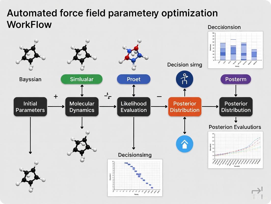
The following diagram illustrates a generalized, automated workflow for Bayesian force field optimization, integrating elements from several research efforts.

Automated Bayesian Force Field Optimization

Protocol 1: Bayesian Optimization of Partial Charges

This protocol is adapted from methods that learn partial charge distributions from ab initio molecular dynamics (AIMD) data [5].

Define System and Prepare Reference Data

• Select Molecular Fragments: Choose small, chemically meaningful fragments representative of the larger system (e.g., acetate, methylammonium) [5].
• Generate AIMD Reference Data: Perform AIMD simulations of each solvated fragment. From the trajectories, extract condensed-phase structural Quantities of Interest (QoIs), such as:
  • Radial distribution functions (RDFs) between solute and solvent atoms.
  • Hydrogen bond counts or order parameters.
  • Ion-pair distance distributions (for charged species) [5].
• Enforce Physical Constraints: Define a truncated normal prior for partial charges, with bounds based on typical force field values and a constraint to maintain the total molecular charge [5].

Build a Surrogate Model

• Run Initial Force Field Simulations: Execute multiple classical molecular dynamics (FFMD) simulations, sampling partial charges from the prior distribution.
• Train Local Gaussian Process (LGP) Surrogate: For each QoI, train an LGP model that maps a set of partial charges to the predicted QoI. This surrogate dramatically accelerates posterior sampling by replacing costly FFMD simulations [5].

Sample the Posterior via MCMC

• Define Likelihood: Use a multivariate Gaussian to quantify the agreement between LGP-predicted QoIs and the AIMD reference data.
• Execute MCMC Sampling: Use a sampler (e.g., No-U-Turn Sampler) to draw samples from the posterior distribution of partial charges. The LGP surrogate enables the efficient evaluation of thousands of candidate parameter sets [5].
• Validate Parameters: Select multiple posterior samples and run full FFMD simulations to confirm they reproduce the AIMD reference data within acceptable error margins (e.g., RDF errors < 5%) [5].

Protocol 2: Model Selection for the 2CLJQ Fluid Model

This protocol uses Bayesian model selection to determine the justified level of complexity in a molecular model, as demonstrated with the two-centered Lennard-Jones + quadrupole (2CLJQ) model [1].

Define Model Hierarchy

Establish a set of nested models with increasing complexity:

• Model M1 (United Atom): Fixed bond length (L) and fixed zero quadrupole moment (Q).
• Model M2 (Anisotropic United Atom): Variable bond length (L) and fixed zero quadrupole moment (Q).
• Model M3 (Anisotropic United Atom + Quadrupole): Variable bond length (L) and variable quadrupole moment (Q) [1].

Specify Priors and Likelihood

• Priors: Assign informative prior distributions to parameters based on previous knowledge or chemical intuition. For example, use a normal distribution for the bond length L centered on a known value from quantum chemistry [1].
• Likelihood: Assume experimental errors are independent and identically distributed, using a Gaussian likelihood to compare simulation outputs to experimental data (e.g., saturated liquid density, vapor pressure, surface tension) [1].

Calculate Bayes Factors via RJMC

• Implement Reversible Jump Monte Carlo (RJMC): Use RJMC to sample simultaneously across the different models and their parameter spaces. This algorithm allows transitions between models while maintaining detailed balance [1].
• Compute Bayes Factors: Estimate the evidence for each model by calculating the Bayes factor (B32) between two models (e.g., M3 and M2). A B32 > 1 supports the more complex model (M3). Interpretation follows scales like Kass and Raftery's (e.g., B32 > 10 is strong evidence) [3] [1].
• Decision: Adopt the most complex model only if the Bayes factor provides positive or strong evidence in its favor, ensuring additional parameters are justified by the data [1].

The Scientist's Toolkit

Table 2: Essential Research Reagents and Computational Tools

Item / Software	Function / Purpose	Application Example	Key Features
Stan / PyMC3	Probabilistic programming languages for flexible Bayesian modeling [3].	Specifying custom likelihoods and priors for force field parameter posteriors.	Hamiltonian Monte Carlo, No-U-Turn Sampler [3]
LGP Surrogate Model	Fast emulator for molecular simulation observables [5].	Accelerating MCMC sampling by predicting RDFs from charges without full MD.	Interpretable, physics-informed priors [5]
Replica-Averaged Forward Model	Bayesian reweighting algorithm for ensemble-averaged data [4].	Refining force field parameters against sparse/noisy experimental observables.	Handles systematic error, infers uncertainty [4]
Mapped Gaussian Process (MGP)	Accelerated Bayesian machine learning force field [6].	Large-scale MD with quantum accuracy and on-the-fly active learning.	Built-in uncertainty, constant evaluation cost [6]
Ab Initio MD (AIMD) Data	High-level reference data for condensed-phase behavior [5].	Providing target RDFs and HB statistics for charge optimization.	Captures many-body and polarization effects [5]

Advanced Methodologies

MCMC Sampling for Conformational Populations

The internal mechanism of MCMC sampling for a method like Bayesian Inference of Conformational Populations (BICePs) can be visualized as follows [4]:

BICePs MCMC Sampling Process

This diagram shows the core cycle of an MCMC algorithm used in methods like BICePs [4]. It samples both conformational states (X) and uncertainty parameters (σ), evaluating the posterior probability which balances a simulation-derived prior against the likelihood of matching experimental data. The process iterates, building up the posterior distribution used for force field validation and refinement [4].

Core Challenges in Traditional Force Field Optimization

Force fields are fundamental to molecular simulations, enabling the study of material properties and dynamic processes from the atomic to the mesoscopic scale. They establish a mathematical relationship between a system's energy and the positions of its atoms, creating a potential energy surface (PES) that is crucial for exploring chemical reactions and material characteristics [7]. The accuracy of this PES directly determines the reliability of simulation outcomes in applications such as drug design, catalyst development, and material science. Traditional force field optimization involves refining parameters to ensure the model faithfully reproduces reference data, which can come from high-level quantum mechanical (QM) calculations or experimental measurements [4] [8]. However, this process is fraught with challenges, including the high dimensionality of parameter space, the competing demands of accuracy and transferability, and the need to properly account for errors and uncertainties in reference data. This document outlines the core challenges within the context of developing automated, robust optimization workflows, with a specific focus on the role of Bayesian inference methods in addressing these issues.

Classification of Force Fields and Their Parameterization Landscape

Understanding the different types of force fields is essential for appreciating their respective optimization challenges. They can be broadly categorized into three groups, each with a distinct approach to modeling the PES.

Table 1: Classification and Characteristics of Major Force Field Types

Force Field Type	Typical Number of Parameters	Interpretability	Primary Optimization Targets	Key Limitations
Classical Force Fields (e.g., CHARMM, OPLS-AA, GAFF) [9] [7]	10 - 100 [7]	High (parameters often have direct physical meaning) [7]	Liquid densities, vaporization enthalpies, vibrational frequencies [8]	Cannot describe bond breaking/formation; limited accuracy for properties not explicitly fitted [7]
Reactive Force Fields (e.g., ReaxFF) [10] [7]	100+ [7]	Medium (complex functional forms) [10]	Reaction energies, barriers, DFT-level structures [10]	Struggles to achieve DFT-level accuracy for new systems; complex parameterization [10]
Machine Learning Force Fields (MLFFs) (e.g., EMFF-2025, Neural Network Potentials) [10] [7]	100,000+ (network weights)	Low ("black box" models)	DFT-level energies and forces for diverse configurations [10]	High computational cost for training; data hunger; limited transferability outside training data [10]

The parameterization strategy differs significantly across these types. Classical force fields are typically optimized using least-squares minimization or global optimization algorithms (e.g., the Levenberg-Marquardt algorithm used for methane [11]) against a limited set of condensed-phase experimental data, such as liquid density (( \rho{\text{liq}} )) and vaporization enthalpy (( \Delta H{\text{vap}} )) [8]. In contrast, reactive force fields and machine learning force fields are heavily parameterized against large datasets derived from Quantum Mechanical (QM) calculations, such as Density Functional Theory (DFT), which provide target values for energies, forces, and charges [10] [7]. The EMFF-2025 potential, for instance, was developed using a transfer learning strategy that leverages a pre-trained model and incorporates minimal new data from DFT calculations, achieving chemical accuracy for a wide range of high-energy materials [10].

Core Challenges in Force Field Optimization

The Accuracy-Transferability Trade-off and Parametric Complexity

A fundamental challenge is the inherent trade-off between a force field's accuracy for specific systems and its transferability to novel compounds or different physical states. Traditional force fields parameterized solely on fluid-phase thermodynamic properties often fail to accurately predict solid-liquid equilibria (SLE). For example, the TraPPE force field, while accurate for liquid-phase properties of methane, exhibited significant deviations (over 17 K) in predicting melting points [11]. Similarly, the OPLS force field has been shown to underestimate the melting point of benzene by 23 K and overestimate that of methanol by approximately 20% [11]. This lack of transferability underscores a critical challenge: a model's performance is inherently limited by the data used for its parameterization.

The complexity of the optimization landscape escalates with the number of parameters. While classical force fields have a relatively low-dimensional space (10-100 parameters), it remains highly correlated and interdependent [4]. Changing a single parameter, such as the Lennard-Jones well depth (( \epsilon )) or radius (( \sigma )), can affect multiple physical properties simultaneously, making it difficult to isolate the effect of a single parameter change [11]. This interdependence is even more pronounced in complex reactive force fields and is extreme in machine learning force fields, where millions of non-physical parameters (network weights) must be optimized [10] [7].

Data-Related Challenges: Uncertainty, Error, and Sparse Observables

Force field refinement must contend with significant uncertainties in both the reference data and the forward models used to predict observables.

• Uncertainty in Reference Data: Both QM calculations and experimental measurements are subject to random and systematic errors [4]. QM methods have intrinsic errors based on the chosen functional and basis set, while experimental data can be sparse and noisy [4] [12]. Many force field optimization algorithms lack a robust mechanism to integrate these multiple sources of uncertainty, leading to overfitting to potentially erroneous data points.

• Sparse and Ensemble-Averaged Data: Experimental observations, such as those from NMR or scattering techniques, are typically ensemble-averaged, representing a weighted mean across a vast number of conformational states [4] [12]. Optimizing a force field against such data is an ill-posed inverse problem, as many different microscopic parameter sets could potentially yield the same macroscopic average. This is further complicated when the experimental data is sparse, providing an incomplete set of restraints for the optimization.

The High Computational Cost of Validation

A force field's performance cannot be assessed solely on its optimization targets; rigorous validation against non-target properties is essential. This process is computationally demanding. For example, validating a force field for liquid membrane applications requires extensive molecular dynamics (MD) simulations to compute properties like density, shear viscosity, interfacial tension, and mutual solubility, which are then benchmarked against experimental data [9]. This validation often reveals shortcomings, as seen with the GAFF and OPLS-AA/CM1A force fields, which overestimated the viscosity of diisopropyl ether (DIPE) by 60-130% [9]. Similarly, the CombiFF-optimized force fields showed good agreement with experiment for many non-target properties but exhibited larger discrepancies for shear viscosity and dielectric permittivity, likely due to the united-atom representation and implicit treatment of electronic polarization [8]. This highlights that the physical formulation of a force field ultimately constrains its achievable accuracy, regardless of parameter tuning.

A Bayesian Inference Protocol for Robust Force Field Optimization

Bayesian Inference of Conformational Populations (BICePs) provides a powerful statistical framework to address the challenges of uncertainty and sparse data [4] [12]. The following protocol outlines its application for force field refinement.

Theoretical Foundation

BICePs samples the full posterior distribution of parameters, which is proportional to the likelihood of the experimental data given the parameters, multiplied by the prior distributions of the parameters [4]: p(X, σ | D) ∝ p(D | X, σ) p(X) p(σ)

Where:

• X represents the conformational states.
• σ represents the uncertainty parameters (nuisance parameters).
• D is the experimental data.
• p(D | X, σ) is the likelihood function.
• p(X) is the prior population from a theoretical model (e.g., a molecular simulation).
• p(σ) is a non-informative prior for the uncertainty.

A key innovation is the use of a replica-averaged forward model [4] [12]. Instead of comparing data to a single simulation snapshot, the forward model prediction is an average over multiple replicas of the system: f_j(X) = (1/N_r) * ∑_{r=1}^{N_r} f_j(X_r). This makes BICePs a maximum-entropy reweighting method that naturally balances experimental information with the prior without needing adjustable regularization parameters [4].

Detailed Experimental Protocol

Step 1: System Setup and Prior Ensemble Generation

• Procedure: Choose the molecular system and the force field parameters to be optimized. Run extensive molecular dynamics (MD) or Monte Carlo (MC) simulations using an initial force field to generate a theoretical prior ensemble. This ensemble provides the initial guess for the conformational populations, p(X).
• Critical Notes: The quality of the prior ensemble influences the efficiency of convergence but not the final result, as BICePs can reweight it significantly. For a lattice model test system, this might involve exhaustive enumeration of states [4].

Step 2: Define Observables and Forward Model

• Procedure: Identify the ensemble-averaged experimental observables D to be used as restraints (e.g., NMR J-couplings, distance measurements from FRET, thermodynamic data). Define the forward model f(X) that calculates the theoretical value of an observable from a given molecular configuration X [12].
• Example: For optimizing Karplus parameters for J-coupling constants, the forward model is the Karplus relation: ^3J(φ) = A cos²(φ) + B cos(φ) + C, where φ is the dihedral angle and A, B, C are the parameters to be optimized [12].

Step 3: Configure BICePs and Sample the Posterior

• Procedure: Use the BICePs algorithm to sample the posterior distribution p(X, σ | D).
  • Likelihood Selection: Choose an appropriate likelihood function. The Student's likelihood model is robust for handling outliers and systematic errors, as it marginalizes over individual uncertainties with a fewer number of parameters [4].
  • MCMC Sampling: Perform Markov Chain Monte Carlo (MCMC) sampling to explore the space of conformational populations X and uncertainty parameters σ. Gradients of the BICePs score with respect to force field parameters can be used to accelerate convergence [4] [12].
• Critical Notes: The number of replicas N_r should be sufficiently large to reduce the standard error of the mean in the replica-averaged forward model.

Step 4: Variational Optimization and Model Selection

• Procedure: Use the BICePs score—a free energy-like quantity that reports the evidence for a model—as the objective function for variational optimization.
  • Optimization: Employ stochastic gradient descent to minimize the BICePs score with respect to the force field parameters θ. The parameter update can be formulated as: θ_trial = θ_old - l_rate ⋅ ∇u + η ⋅ N(0,1), where l_rate is the learning rate and η is noise to escape local minima [4] [12].
  • Validation: The optimized force field must be validated against a held-out set of experimental data or properties not used in the optimization (e.g., transport properties, SLE data) to ensure its transferability [11] [9] [8].

Table 2: Research Reagent Solutions for Bayesian Force Field Optimization

Reagent / Resource	Type	Function in the Protocol	Example Use Case
BICePs Algorithm	Software	Core engine for sampling the posterior and computing the BICePs score [4].	Force field validation and refinement against ensemble data [4].
Replica-Averaged Forward Model	Computational Method	Predicts ensemble-averaged observables from multiple conformational replicas, reducing overfitting [4] [12].	Calculating expected J-coupling constants from an ensemble of protein structures [12].
Student's Likelihood Model	Statistical Model	Likelihood function robust to outliers and systematic error; limits number of uncertainty parameters [4].	Down-weighting the influence of erroneous or inconsistent data points during refinement [4].
QM Reference Data (e.g., from DFT)	Dataset	Provides high-accuracy target data for parameterizing reactive and ML force fields [10] [7].	Training the EMFF-2025 neural network potential for energetic materials [10].
Experimental Ensemble Data (e.g., NMR, Thermodynamic)	Dataset	Provides physical restraints for refining force field parameters against real-world observations [4] [8].	Optimizing force fields to reproduce liquid densities and vaporization enthalpies [8].

Diagram 1: Workflow for Bayesian Force Field Optimization. The process integrates prior simulation data with experimental observations to sample a posterior distribution, which is then used to variationally optimize force field parameters (θ), followed by essential validation.

The optimization of traditional force fields is constrained by significant challenges, including the accuracy-transferability trade-off, high-dimensional and correlated parameter spaces, and the pervasive presence of uncertainty in reference data. The Bayesian Inference of Conformational Populations (BICePs) protocol presented here offers a robust, automated framework to address these issues. By explicitly sampling posterior distributions and leveraging replica-averaged forward models with robust likelihoods, BICePs facilitates force field refinement that is resilient to data sparsity and errors. This approach, which can be integrated with both classical and machine learning potentials, represents a promising path toward more reliable and predictive molecular simulations for drug development and materials science.

Bayesian Inference of Conformational Populations (BICePs) is a statistically rigorous algorithm designed to reconcile theoretical predictions of molecular conformational ensembles with sparse and/or noisy experimental measurements [13]. Developed to address the challenges of characterizing structurally heterogeneous molecules, BICePs operates within a Bayesian framework to reweight conformational state populations as a post-simulation processing step [13] [14]. This approach has proven particularly valuable for studying natural product macrocycles, peptidomimetics, and other foldamers where conventional structural determination methods face limitations [13].

A key innovation of BICePs is its ability to perform objective model selection through a quantity known as the BICePs score, which reflects the integrated posterior evidence for a given model [14]. This capability, combined with proper implementation of reference potentials, distinguishes BICePs from earlier Bayesian inference methods like Inferential Structure Determination (ISD) [13]. The algorithm has evolved significantly since its inception, with BICePs v2.0 now supporting diverse experimental observables and providing user-friendly tools for data preparation, processing, and posterior analysis [15] [16].

Theoretical Foundation

Bayesian Inference Framework

BICePs models a posterior distribution ( P(X|D) ) of conformational states ( X ), given experimental data ( D ). According to Bayes' theorem, this posterior probability is proportional to the product of a likelihood function and a prior distribution [13]:

[ P(X|D) \propto Q(D|X)P(X) ]

Here, ( P(X) ) represents the prior distribution of conformational populations derived from theoretical modeling, such as molecular simulations. The likelihood function ( Q(D|X) ) quantifies how well a given conformation ( X ) agrees with experimental measurements and typically assumes a normally-distributed error model [13]:

[ Q(D|X,\sigma) = \prodj \frac{1}{\sqrt{2\pi\sigma^2}} \exp\left(-[rj(X) - r_j^{\text{exp}}]^2 / 2\sigma^2\right) ]

where ( rj(X) ) are observables back-calculated from the theoretical model, ( rj^{\text{exp}} ) are experimental values, and ( \sigma ) represents uncertainty parameters that account for both experimental error and conformational heterogeneity [13].

Reference Potentials

A crucial advancement in BICePs is the proper implementation of reference potentials ( Q_{\text{ref}}(r) ), which account for the information content of experimental restraints [13] [14]. The modified posterior probability becomes [13]:

[ P(X|D) \propto \left[ \frac{Q(r(X)|D)}{Q_{\text{ref}}(r(X))} \right] P(X) ]

The reference potential represents the distribution of observables in the absence of experimental information, ensuring that restraints are weighted according to their informativeness [14]. For example, a distance restraint between residues far apart in sequence provides more information than one between nearby residues, and appropriate reference potentials prevent introduction of unnecessary bias when multiple non-informative restraints are used [13] [14].

The BICePs Score for Model Selection

The BICePs score is a Bayes factor-like quantity that enables quantitative model selection [14]. It is computed as the free energy of introducing experimental restraints:

[ \text{BICePs score} = -\ln Z{\text{posterior}} + \ln Z{\text{prior}} ]

where ( Z{\text{posterior}} ) and ( Z{\text{prior}} ) are the partition functions of the posterior and prior distributions, respectively [14]. This score represents the integrated evidence for a model given the experimental data, with more negative values indicating models that better agree with experiments [14] [4].

Table 1: Key Theoretical Concepts in BICePs

Concept	Mathematical Representation	Role in BICePs
Prior Distribution	( P(X) )	Represents theoretical predictions of conformational populations from simulations
Likelihood Function	( Q(D|X,\sigma) )	Quantifies agreement between conformational states and experimental data
Posterior Distribution	( P(X|D) )	Balanced estimate of conformational populations considering both theory and experiment
Reference Potential	( Q_{\text{ref}}(r) )	Accounts for inherent distributions of observables without experimental bias
BICePs Score	( -\ln Z{\text{posterior}} + \ln Z{\text{prior}} )	Enables model selection by quantifying total evidence for a model

BICePs in Automated Force Field Parameterization

Variational Optimization Framework

Recent advancements have extended BICePs to perform automated force field refinement through variational minimization of the BICePs score [4]. This approach treats force field parameters as adjustable variables ( \theta ) and optimizes them by minimizing the BICePs score, which serves as an objective function that naturally regularizes against overfitting [4]:

[ \theta^* = \arg\min_{\theta} \left[ -\ln \int P(X,D|\theta) dX \right] ]

This variational framework leverages gradient information for efficient optimization in high-dimensional parameter spaces [4]. The derivation of first and second derivatives of the BICePs score enables the use of sophisticated optimization algorithms that converge more rapidly than derivative-free approaches [4].

Handling Systematic Errors and Outliers

BICePs incorporates specialized likelihood functions robust to systematic errors and experimental outliers [4]. The Student's model, for instance, marginalizes uncertainty parameters for individual observables while assuming mostly uniform noise levels with occasional erratic measurements [4]. This approach limits the number of uncertainty parameters that need sampling while effectively capturing outliers [4].

For replica-averaged simulations, the uncertainty parameter ( \sigmaj ) combines Bayesian error ( \sigmaj^B ) and standard error of the mean ( \sigma_j^{\text{SEM}} ) [4]:

[ \sigmaj = \sqrt{(\sigmaj^B)^2 + (\sigma_j^{\text{SEM}})^2} ]

where ( \sigma_j^{\text{SEM}} ) is estimated from the finite sample of replicas and decreases with the square root of the number of replicas [4].

Application to Forward Model Parameterization

BICePs has also been adapted for empirical forward model parameterization [17]. Two novel methods have been developed:

• Nuisance parameter integration: Treats forward model parameters as nuisance parameters and integrates over them in the full posterior distribution [17].
• Variational minimization: Employs BICePs score minimization to optimize parameters, applicable to any differentiable forward model [17].

This approach has been successfully demonstrated in refining Karplus parameters for J-coupling constant predictions, showing improved accuracy for both toy model systems and human ubiquitin [17].

Computational Protocols and Implementation

BICePs Workflow

The following diagram illustrates the standard BICePs workflow for conformational ensemble refinement:

BICePs Software Specifications

BICePs v2.0 is implemented as a free, open-source Python package that provides comprehensive tools for ensemble reweighting [15] [16]. Key features include:

Table 2: BICePs v2.0 Software Capabilities

Feature	Description	Supported Data Types
Experimental Observables	NMR data processing	NOE distances, J-couplings, chemical shifts, HDX protection factors [15] [16]
Sampling Methods	Posterior distribution sampling	Markov Chain Monte Carlo (MCMC) [13]
Uncertainty Quantification	Error model estimation	Nuisance parameter sampling for σ values [13] [14]
Analysis Tools	Posterior analysis and visualization	Convergence assessment, statistical significance evaluation [15]
Model Selection	BICePs score calculation	Free energy estimation for model comparison [14]

Protocol for Force Field Parameter Optimization

The following workflow illustrates the extended BICePs protocol for automated force field parameter optimization:

Step-by-Step Implementation:

• Initialization: Begin with initial force field parameters and experimental reference data [4].

• Ensemble Generation: Perform molecular simulations to generate conformational ensembles using current force field parameters [4].

• BICePs Score Calculation: Compute the BICePs score comparing ensemble predictions with experimental data [14] [4].

• Gradient Estimation: Calculate derivatives of the BICePs score with respect to force field parameters using adjoint methods or automatic differentiation [4].

• Parameter Update: Adjust force field parameters using gradient-based optimization algorithms to minimize the BICePs score [4].

• Convergence Check: Repeat steps 2-5 until the BICePs score stabilizes and parameters converge [4].

• Validation: Assess optimized force field performance on independent test systems not used during parameter optimization [4].

The Scientist's Toolkit

Table 3: Essential Research Reagents and Computational Tools

Tool/Resource	Function	Application Context
BICePs v2.0 Software	Open-source Python package for Bayesian ensemble reweighting	Core algorithm implementation [15] [16]
Molecular Dynamics Engine	Generate conformational ensembles	Prior distribution sampling (e.g., GROMACS, OpenMM) [4]
NMR Data Processing	Prepare experimental observables	Input data preparation for NOE, J-couplings, chemical shifts [15]
Markov Chain Monte Carlo	Posterior distribution sampling	Uncertainty quantification and ensemble refinement [13]
Automatic Differentiation	Gradient computation for optimization	Force field parameter sensitivity analysis [4]
Reference Potential Database	Baseline distributions for observables	Proper normalization of experimental restraints [13] [14]

BICePs provides a powerful framework for reconciling theoretical predictions with experimental measurements through Bayesian inference. Its core innovations—proper reference potential implementation and the BICePs score for model selection—enable both conformational ensemble refinement and force field parameter optimization. Recent extensions toward automated parameter optimization using variational methods and robust error handling demonstrate BICePs' evolving capabilities in addressing key challenges in computational biophysics and molecular design.

The integration of BICePs into automated force field parameterization workflows represents a significant advancement for the field, offering a principled approach to force field development that naturally accounts for experimental uncertainties and systematic errors. As molecular simulations continue to play an increasingly important role in drug discovery and materials design, BICePs provides an essential bridge between theoretical modeling and experimental validation.

Accurate molecular force fields are critical for reliable simulations in structural biology and drug design. However, force field parameterization is fundamentally challenged by multiple sources of uncertainty, including sparse or noisy experimental data and approximations in computational models [4]. Bayesian inference provides a powerful framework for addressing these challenges through the explicit treatment of uncertainty. This application note examines the role of nuisance parameters and specialized error models within automated force field optimization workflows, with a focus on practical implementation for research scientists.

Nuisance parameters enable the quantification of uncertainty in both experimental measurements and forward model predictions, while robust likelihood functions automatically identify and down-weight outliers affected by systematic error [4] [12]. The integration of these elements into methods like Bayesian Inference of Conformational Populations (BICePs) allows for the simultaneous refinement of force field parameters and quantification of uncertainty, leading to more reliable and interpretable models [4] [12].

Quantitative Analysis of Bayesian Error Models

Table 1: Key Likelihood Functions and Error Models in Bayesian Force Field Optimization

Model Name	Mathematical Formulation	Handled Uncertainty	Key Advantages
Gaussian Likelihood [4]	( p(D \mid X, \sigma) \propto \prod{j=1}^{Nj} \frac{1}{\sqrt{2\pi\sigmaj^2}} \exp\left[-\frac{(dj - fj(\mathbf{X}))^2}{2\sigmaj^2}\right] )	Random error	Simple, widely applicable; works with replica-averaged forward model.
Student's t Likelihood [4]	Derived by marginalizing individual uncertainties ( \sigmaj ) conditioned on a typical uncertainty ( \sigma0 ).	Random error and systematic outliers	Robust to outliers; limits number of uncertainty parameters needing sampling.
Replica-Averaged Forward Model [4] [12]	( \sigmaj = \sqrt{(\sigmaj^B)^2 + (\sigmaj^{SEM})^2} ) where ( \sigmaj^{SEM} = \sqrt{ \frac{1}{N} \sumr^N (fj(Xr) - \langle fj(\mathbf{X}) \rangle)^2 } )	Finite sampling error and experimental noise	Separately accounts for Bayesian uncertainty (( \sigma^B )) and standard error of the mean (( \sigma^{SEM} )) from finite replica sampling.

Table 2: Comparison of Bayesian Force Field Optimization Frameworks

Framework	Core Objective	Treatment of Nuisance Parameters	Representative Applications
BICePs [4] [12]	Force field refinement and model selection against ensemble-averaged data.	Sampled via MCMC; includes conformational states ( X ) and experimental uncertainties ( \sigma ).	Protein lattice models; Karplus parameter optimization for ubiquitin [12].
BioFF [2]	Iterative force field parameterization using ensemble refinement.	Regularization via entropic prior on ensemble and simplified prior on force field parameters.	Simple polymer model using label-distance data [2].
Bayesian Partial Charge Optimization [5]	Learning charge distributions from ab initio MD data.	Uncertainty in parameters is inherent to the posterior distribution; uses surrogate models for efficiency.	18 biologically relevant molecular fragments; calcium binding to troponin [5].

Experimental Protocol: BICePs for Force Field Optimization

This protocol outlines the procedure for automating force field parameter refinement using the BICePs algorithm, based on the methodology described by Raddi et al. [4] [12].

Stage 1: System Preparation and Prior Definition

• Generate a Prior Conformational Ensemble: Perform molecular dynamics (MD) simulations using an initial force field to generate a structural ensemble. This provides the prior distribution of conformational populations, ( p(X) ) [4] [12].
• Define Observables and Forward Model: Identify the set of experimental observables ( D ) (e.g., NMR J-couplings, distance measurements). Establish a forward model ( f(X) ) that computes these observables from any molecular configuration ( X ) [12].

Stage 2: BICePs Setup and Configuration

• Specify Nuisance Parameters: Define the uncertainty parameters ( \sigma_j ) for each experimental observable. These will be treated as nuisance parameters and sampled [4].
• Select Likelihood Function:
  • For data with primarily random error, the Gaussian likelihood is appropriate.
  • For datasets suspected to contain outliers or systematic errors, the Student's t likelihood is recommended, as it marginalizes over individual uncertainties and is more robust [4].
• Implement Replica-Averaging: Configure the replica-averaged forward model, ( fj(\mathbf{X}) = \frac{1}{Nr}\sum{r}^{Nr} fj(Xr) ), where ( N_r ) is the number of replicas. This accounts for finite sampling error in the simulation [4] [12].

Stage 3: Sampling and Optimization Execution

• Sample the Posterior: Use Markov Chain Monte Carlo (MCMC) sampling to draw from the full posterior distribution: ( p(\mathbf{X}, \bm{\sigma}, \theta \mid D) \propto p(D \mid g(\mathbf{X}, \theta), \bm{\sigma}) p(\mathbf{X}) p(\bm{\sigma}) p(\theta) ) This samples conformational states ( \mathbf{X} ), nuisance parameters ( \bm{\sigma} ), and force field parameters ( \theta ) simultaneously [4] [12].
• Variational Optimization (Alternative): Alternatively, optimize force field parameters by minimizing the BICePs score, a free energy-like quantity. This variational approach can leverage gradient information for faster convergence in high-dimensional parameter spaces [4] [12]. ( \theta{\text{new}} = \theta{\text{old}} - \text{lrate} \cdot \nabla u + \eta \cdot \mathcal{N}(0,1) ) This update incorporates stochastic noise ( \eta ) to escape local minima [12].

Stage 4: Validation and Analysis

• Convergence Diagnostics: Monitor MCMC chains for convergence of both force field parameters ( \theta ) and nuisance parameters ( \sigma ).
• Model Validation: Validate the refined force field by assessing its performance on independent experimental data or observables not used in the training set.
• Uncertainty Quantification: Report the posterior distributions of the optimized parameters, which provide natural confidence intervals [5].

Workflow Visualization

The Scientist's Toolkit

Table 3: Essential Research Reagents and Computational Tools

Tool/Reagent	Function in Workflow	Implementation Notes
Conformational Ensemble [4] [12]	Serves as the prior distribution ( p(X) ) for Bayesian inference.	Typically generated from MD simulation; should broadly cover conformational space.
Forward Model [12]	Computes theoretical observables ( f(X) ) from structures for comparison with experiment.	Can be empirical (e.g., Karplus equation) or machine learning-based; must be differentiable for gradient-based optimization.
BICePs Software [4] [12]	Implements the core Bayesian inference algorithm, MCMC sampling, and BICePs score calculation.	Key features: replica-averaging, robust likelihoods, and gradient calculation for optimization.
MCMC Sampler [4] [5]	Samples the posterior distribution of parameters and nuisance variables.	Critical for uncertainty quantification; requires convergence diagnostics.
Ab Initio MD Data [5]	Provides high-quality reference data for parameterizing force fields against quantum-mechanical targets.	Used as a condensed-phase benchmark; captures many-body interactions and polarization effects.

Handling Sparse, Noisy, and Ensemble-Averaged Experimental Data

Automated force field optimization represents a paradigm shift in molecular simulation, moving beyond traditional manual parameterization towards robust, data-driven workflows. Within this domain, a central challenge is the effective utilization of experimental data that is often limited in quantity (sparse), contains significant measurement errors (noisy), and provides only averaged structural information (ensemble-averaged). Bayesian inference frameworks have emerged as particularly powerful tools for addressing these challenges, as they explicitly account for uncertainty in both parameters and data. These methods enable researchers to extract maximum information from limited experimental observations while avoiding overfitting and providing natural mechanisms for quantifying confidence in the resulting models. This application note examines the key advantages of Bayesian approaches for handling difficult data scenarios and provides detailed protocols for implementation in force field development pipelines, particularly relevant for drug discovery applications where experimental data may be scarce or expensive to acquire.

Key Advantages of Bayesian Methods for Challenging Data

Bayesian methods provide several distinct advantages over traditional optimization approaches when working with sparse, noisy, and ensemble-averaged experimental data. These advantages stem from the probabilistic nature of Bayesian inference, which treats both parameters and data as probability distributions rather than fixed values.

Table 1: Advantages of Bayesian Methods for Different Data Challenges

Data Challenge	Bayesian Approach	Key Advantage	Representative Method
Sparse Data	Prior distributions regularize inference	Prevents overfitting; incorporates physical constraints	Bayesian Inference of Conformational Populations (BICePs) [4]
Noisy Data	Explicit error models with nuisance parameters	Separates experimental error from model discrepancy	Student's t-likelihood for outlier resilience [4]
Ensemble-Averaged Data	Replica-averaged forward models	Connects single structures to experimental observables	Maximum Entropy reweighting [4]
Systematic Errors	Hierarchical error models	Automatically detects and down-weights outliers	Marginalized uncertainty parameters [4]
Transferability	Uncertainty quantification	Natural confidence intervals for parameters	Posterior distribution analysis [5]

Formal Statistical Treatment of Uncertainty

Unlike conventional force field optimization methods that typically treat experimental uncertainties as fixed, known quantities, Bayesian methods formally incorporate uncertainty as part of the inference problem. The BICePs algorithm, for instance, treats the extent of uncertainty in experimental observables (σ) as nuisance parameters that are sampled alongside conformational populations [4]. This approach uses a Bayesian posterior of the form:

[ p(X,\sigma|D) \propto p(D|X,\sigma)p(X)p(\sigma) ]

where (X) represents conformational states, (D) is the experimental data, and (\sigma) captures uncertainties in measurements. The Jeffreys prior (p(\sigma) \sim \sigma^{-1}) provides a non-informative starting point for uncertainty estimation [4]. This formal treatment means that rather than simply minimizing discrepancies between simulation and experiment, the algorithm jointly infers both the most likely conformational populations and the most likely extent of experimental error.

Robustness to Outliers and Systematic Errors

Bayesian methods can incorporate specialized likelihood functions that provide exceptional resilience to problematic data points. The Student's likelihood model implements a data error model that marginalizes uncertainty parameters for individual observables, operating under the assumption that most measurements share a similar noise level except for a few erratic measurements [4]. This approach automatically detects and down-weights outliers without requiring manual intervention or pre-filtering of data. The mathematical derivation involves a model where uncertainties for particular observables (\sigmaj) are distributed about some typical uncertainty (\sigma0) according to a conditional probability (p(\sigmaj|\sigma0)), which is then marginalized to derive a posterior with a single uncertainty parameter [4]. This provides significant advantages for drug development applications where experimental conditions may introduce systematic errors that are difficult to characterize in advance.

Natural Regularization for Sparse Data

The incorporation of prior information in Bayesian methods provides inherent regularization that prevents overfitting when working with limited data. This is particularly valuable in force field parameterization where the number of adjustable parameters may be large relative to the available experimental data. Bayesian approaches maintain a balance between fitting the experimental data and maintaining physically reasonable parameter values through the prior distribution [5]. The resulting posterior distributions provide not just single "best-fit" parameters but entire probability landscapes, enabling researchers to understand which parameters are well-constrained by the data and which remain uncertain [5]. This uncertainty quantification is crucial for establishing the domain of applicability of force fields, especially when extending to novel molecular systems in drug discovery.

Quantitative Assessment of Method Performance

Table 2: Performance Metrics for Bayesian Force Field Optimization

Performance Metric	Traditional Methods	Bayesian Methods	Experimental Validation
Uncertainty Quantification	Limited or post-hoc	Native to inference	Posterior distributions provide natural confidence intervals [5]
Outlier Resilience	Manual exclusion required	Automatic detection	Student's likelihood minimizes impact of erratic measurements [4]
Convergence Stability	Sensitive to initial parameters	More robust to initialization	MCMC sampling explores parameter space more completely [4] [5]
Computational Cost	Lower per iteration	Higher per iteration	Surrogate models (e.g., LGPs) can accelerate sampling [5]
Transferability Assessment	Limited insights	Built-in uncertainty propagation	Posterior predictive checks validate transferability [5]

Experimental Protocols

Protocol: BICePs with Replica-Averaged Forward Model

Purpose: To reconcile molecular simulations with sparse or noisy ensemble-averaged experimental measurements while automatically determining appropriate uncertainty parameters.

Materials and Equipment:

• Molecular dynamics simulation software (e.g., GROMACS, NAMD, OpenMM)
• BICePs software package (Python implementation)
• Experimental data (NMR, FRET, or other ensemble-averaged measurements)
• High-performance computing cluster

Procedure:

• Generate Prior Ensemble: Run molecular dynamics simulations to generate an initial structural ensemble. This serves as the prior distribution (p(X)) [4].
• Define Forward Model: Implement mathematical functions that calculate experimental observables from atomic coordinates (e.g., J-couplings, chemical shifts, distance measurements) [4].
• Set Up Replica-Averaged Likelihood: Configure the replica-averaged forward model with Gaussian likelihood: [ p(\mathbf{X},\bm{\sigma}|D) \propto \prod{r=1}^{Nr}\left{p(Xr)\prod{j=1}^{Nj}\frac{1}{\sqrt{2\pi\sigmaj^2}}\exp\left[-\frac{(dj-fj(\mathbf{X}))^2}{2\sigmaj^2}\right]p(\sigmaj)\right} ] where (fj(\mathbf{X}) = \frac{1}{Nr}\sum{r}^{Nr}fj(Xr)) is the replica-averaged forward model prediction [4].
• Configure MCMC Sampling: Set up Markov chain Monte Carlo sampling to sample simultaneously from conformational states and uncertainty parameters.
• Run Sampling Phase: Execute extended MCMC sampling to obtain posterior distributions of conformational populations and uncertainty parameters.
• Calculate BICePs Score: Compute the BICePs score for model selection, which represents the free energy of turning on conformational populations under experimental restraints [4].
• Validate with Synthetic Data: Test the workflow using synthetic data with known ground truth to verify proper implementation.

Troubleshooting Tips:

• If convergence is slow, consider reducing the number of replicas or adjusting MCMC proposal distributions.
• If uncertainty parameters grow excessively large, check for systematic discrepancies between forward model predictions and experimental data.
• For better performance with outliers, implement the Student's likelihood model instead of Gaussian likelihood.

Protocol: Bayesian Force Field Optimization with AIMD Reference

Purpose: To optimize force field parameters using ab initio molecular dynamics data as reference within a Bayesian framework, providing uncertainty quantification for parameters.

Materials and Equipment:

• Ab initio molecular dynamics software (e.g., CP2K, VASP)
• Classical molecular dynamics software (e.g., GROMACS, OpenMM)
• Bayesian inference software with Gaussian process capabilities
• High-performance computing resources

Procedure:

• Generate AIMD Reference Data: Run ab initio molecular dynamics simulations for target molecular fragments in explicit solvent to capture condensed-phase behavior [5].
• Extract Quantities of Interest: Calculate radial distribution functions, hydrogen bond counts, and other structural properties from AIMD trajectories as reference data [5].
• Define Parameter Priors: Establish physically motivated prior distributions for force field parameters (e.g., truncated normal distributions for partial charges) [5].
• Train Surrogate Model: Develop local Gaussian process surrogate models that map force field parameters to structural quantities of interest, bypassing the need for full MD simulations during inference [5].
• Set Up Bayesian Inference: Configure the likelihood function to measure agreement between classical MD and AIMD reference data.
• Sample Posterior Distribution: Use MCMC sampling to explore the posterior distribution of force field parameters.
• Validate Optimized Force Field: Run validation simulations with the optimized parameters and compare against experimental data not used in training [5].

Troubleshooting Tips:

• If surrogate model predictions are inaccurate, increase the training set size for the Gaussian process.
• If MCMC mixing is poor, consider adjusting proposal distributions or using gradient-based samplers.
• If force field performance is unsatisfactory on validation tests, reconsider the parameter prior distributions or the choice of reference data.

The Scientist's Toolkit: Research Reagent Solutions

Table 3: Essential Computational Tools for Bayesian Force Field Optimization

Tool/Resource	Type	Function in Workflow	Implementation Notes
BICePs	Software package	Bayesian inference of conformational populations	Handles replica-averaged forward models; provides BICePs score for model selection [4]
ForceBalance	Optimization framework	Systematic force field parameter optimization	Supports multiple reference data types; includes regularization [18]
Local Gaussian Process (LGP)	Surrogate model	Accelerates Bayesian inference	Predicts structural properties from parameters faster than full MD [5]
Replica Exchange MD	Sampling enhancement	Improves conformational sampling	Provides better prior ensembles for Bayesian inference
Student's Likelihood	Statistical model	Robustness to outliers	Alternative to Gaussian likelihood; marginalizes individual uncertainties [4]
Ab Initio MD	Reference data generator	Provides training data for force field optimization	Captures condensed-phase behavior with electronic structure accuracy [5]

Discussion

The application of Bayesian methods to force field optimization represents a significant advancement in molecular simulation, particularly for scenarios involving sparse, noisy, or ensemble-averaged experimental data. These approaches transform the fundamental nature of parameterization from a deterministic optimization problem to a probabilistic inference problem, with several important implications for computational drug discovery.

The explicit treatment of uncertainty makes Bayesian methods particularly valuable in early-stage drug development where experimental data may be limited. By quantifying uncertainty in force field parameters, researchers can make more informed decisions about which simulation results can be trusted and which require experimental verification. The natural regularization provided by prior distributions helps prevent overfitting to limited datasets, producing more transferable force fields that perform better on novel molecular systems [5].

The robustness to outliers and systematic errors provided by specialized likelihood functions, such as the Student's model in BICePs, reduces the need for manual data curation and enables more automated workflows [4]. This is particularly valuable in high-throughput settings where manual inspection of all experimental data points is impractical. The ability to automatically detect and down-weight problematic measurements while still extracting information from the remaining data represents a significant efficiency improvement over traditional methods.

For drug development professionals, these Bayesian approaches offer a more rigorous statistical foundation for leveraging expensive experimental data. The quantification of uncertainty provides natural stopping criteria for parameterization efforts - once parameter uncertainties are reduced below functionally significant thresholds. Furthermore, the posterior distributions of parameters enable more robust sensitivity analyses, identifying which parameters most strongly influence key simulation outcomes relevant to drug binding or stability.

As force field development continues to evolve, Bayesian methods provide a natural framework for incorporating diverse data sources - from quantum mechanical calculations to various experimental measurements - while properly accounting for the different uncertainties associated with each data type. This unified approach to force field parameterization will play an increasingly important role in developing the next generation of molecular models for computer-aided drug design.

Methodological Workflows: Implementing Bayesian Optimization from Theory to Practice

Accurate molecular force fields are fundamental to the predictive power of molecular simulations in computational chemistry and structural biology. The parameterization of these force fields, however, presents a significant challenge due to high-dimensional parameter spaces, interdependent parameters, and the sparse, noisy nature of experimental data used for validation [19] [2]. Bayesian Inference of Conformational Populations (BICePs) addresses these challenges through a statistically rigorous framework that reconciles theoretical predictions with experimental measurements [14]. A key innovation within this framework is the BICePs score, a free energy-like quantity that enables both model selection and variational optimization of force field parameters [19] [12]. This application note details the theoretical foundation, practical implementation, and experimental protocols for using the BICePs score in automated force field parameter optimization workflows.

Theoretical Foundation of the BICePs Score

Bayesian Inference of Conformational Populations

BICePs employs a Bayesian framework to infer the posterior distribution of conformational states ( X ) and experimental uncertainty parameters ( \sigma ), given experimental data ( D ) [19] [14]: [ p(X, \sigma | D) \propto \underbrace{p(D | X, \sigma)}{\text{likelihood}} \underbrace{p(X)}{\text{prior}} \underbrace{p(\sigma)}_{\text{prior}} ] Here, the prior ( p(X) typically comes from a theoretical model or molecular simulation, while the likelihood function ( p(D | X, \sigma) quantifies the agreement between forward model predictions ( f(X) and experimental observations [19]. The inclusion of uncertainty parameters ( \sigma ) as nuisance variables allows BICePs to handle random and systematic errors in experimental data without requiring prior error estimates [12] [4].

The BICePs Score as a Model Selection Metric

The BICePs score is defined as the negative logarithm of the marginalized posterior probability [14]: [ \text{BICePs score} = -\ln \int p(D | X, \sigma) p(X) p(\sigma) dX d\sigma ] In practice, this is computed as the free energy change associated with "turning on" the experimental restraints [19] [4]. This score represents the total evidence for a model given the experimental data, providing an unequivocal metric for model selection [14]. Lower BICePs scores indicate models whose predicted ensembles are more consistent with experimental observations.

Table 1: Interpretation of BICePs Score Values in Model Assessment

BICePs Score Range	Model Consistency with Data	Recommended Action
Significantly Lower	High consistency	Preferred model for parameterization
Similar Values	Comparable consistency	Further refinement or additional data needed
Significantly Higher	Low consistency	Model rejection or substantial revision

Advancements in BICePs Score Calculation

Recent enhancements to BICePs have equipped it with a replica-averaging forward model, transforming it into a maximum-entropy (MaxEnt) reweighting method [12] [4]. This approach uses replica-averaged forward model predictions: [ fj(\mathbf{X}) = \frac{1}{Nr} \sum{r}^{Nr} fj(Xr) ] where ( N_r ) is the number of replicas. This formulation eliminates the need for adjustable regularization parameters to balance experimental information with the prior [12]. The BICePs score derived from this enhanced method contains inherent regularization, making it particularly powerful for variational optimization [19].

Variational Optimization Using the BICePs Score

Optimization Framework

The BICePs score serves as a powerful objective function for variational optimization of force field parameters [19]. Consider a force field with parameters ( \mathbf{c} = (c1, c2, \ldots, cm) ) that we wish to optimize. The optimization problem can be formulated as: [ \mathbf{c}^* = \arg \min{\mathbf{c}} \left[ \text{BICePs score}(\mathbf{c}) \right] ] where ( \mathbf{c}^* ) represents the optimal parameter set. This approach enables automated force field refinement while simultaneously sampling the full distribution of uncertainties [19].

Gradient-Based Optimization

For efficient optimization in high-dimensional parameter spaces, BICePs utilizes gradient information [12]. The first and second derivatives of the BICePs score with respect to force field parameters enable efficient exploration of complex parameter landscapes. The parameter update mechanism follows: [ \mathbf{c}{\text{trial}} = \mathbf{c}{\text{old}} - l{\text{rate}} \cdot \nabla u + \eta \cdot \mathcal{N}(0,1) ] where ( l{\text{rate}} ) is the learning rate, ( \nabla u ) is the gradient of the objective function, and ( \eta ) introduces stochastic noise to facilitate escape from local minima [12]. This gradient-based approach significantly accelerates convergence, particularly for higher-dimensional optimization problems [12].

The following diagram illustrates the complete variational optimization workflow using the BICePs score:

Key Research Reagents and Computational Tools

Table 2: Essential Research Reagents and Computational Tools for BICePs Optimization

Tool/Reagent	Function in BICePs Workflow	Implementation Notes
BICePs Software	Core algorithm for posterior sampling and score calculation	BICePs v2.0 provides improved user interface and extensibility [20]
Molecular Dynamics Engine	Generates prior conformational ensembles	GROMACS, AMBER, or OpenMM typically used [21]
Reference Potentials	Corrects for bias from non-informative restraints	Polymer models for chain molecules; maximum-entropy distributions for macrocycles [14]
Gradient Calculation	Enables efficient parameter optimization	First and second derivatives of BICePs score accelerate convergence [12]
Enhanced Likelihood Functions	Handles outliers and systematic errors	Student's t-model marginalizes uncertainty parameters for robust error handling [4]

Experimental Protocol: Force Field Parameter Optimization

This protocol outlines the steps for optimizing force field parameters using variational minimization of the BICePs score, demonstrated for a 12-mer HP lattice model and all-atom systems [19] [14].

Step-by-Step Procedure

Step 1: Initial Ensemble Generation

• Simulate conformational ensemble using initial force field parameters ( \mathbf{c}_0 ) [2].
• Ensure adequate sampling of conformational states ( X ) to represent the equilibrium distribution.
• Calculate theoretical observables ( f(X) ) from the ensemble using appropriate forward models.

Step 2: Experimental Data Preparation

• Compile ensemble-averaged experimental measurements ( D = {d1, d2, \ldots, d_N} ) (e.g., NMR observables, distance measurements) [19] [14].
• Identify potential sources of error but note that precise error estimates are not required as BICePs treats uncertainties as nuisance parameters [4].

Step 3: BICePs Score Calculation

• Implement replica-averaged forward model using sufficient replicas (( Nr )) to minimize standard error [12]: [ \sigmaj^{\text{SEM}} = \sqrt{\frac{1}{N} \sum{r}^{N} (fj(Xr) - \langle fj(\mathbf{X}) \rangle)^2} ]
• Sample the full posterior distribution using Markov Chain Monte Carlo (MCMC) over conformational states ( X ) and uncertainty parameters ( \sigma ) [19] [14].
• Compute BICePs score as the free energy of applying experimental restraints.

Step 4: Parameter Optimization Loop

• Calculate gradients of the BICePs score with respect to force field parameters [12].
• Update parameters using gradient-based optimization: [ \mathbf{c}{\text{new}} = \mathbf{c}{\text{old}} - l_{\text{rate}} \cdot \nabla (\text{BICePs score}) + \eta \cdot \mathcal{N}(0,1) ]
• Repeat Steps 1-3 with updated parameters until convergence criteria are met.

Step 5: Validation and Model Selection

• Compare BICePs scores across different force field models [14].
• Select model with lowest BICePs score as the optimal parameterization.
• Validate optimized force field against independent experimental data not used in optimization.

Critical Steps and Troubleshooting

• Convergence Monitoring: Ensure MCMC sampling reaches equilibrium by monitoring trace plots of key parameters [14].
• Gradient Stability: Adjust learning rate ( l_{\text{rate}} ) and noise term ( \eta ) to balance convergence speed and stability [12].
• Systematic Error Handling: Employ Student's likelihood model to automatically detect and down-weight outliers [4].

Application Examples and Case Studies

Lattice Model Demonstration

In a proof-of-concept study, BICePs was used to optimize interaction parameters for a 12-mer HP lattice model using ensemble-averaged distance measurements [19]. The method successfully identified correct energy parameters despite significant experimental noise and sparse data, demonstrating robustness in the presence of random and systematic errors [19].

All-Atom Protein Force Field Optimization

BICePs has been applied to optimize Karplus parameters for J-coupling constant predictions in human ubiquitin [12]. The approach successfully refined six distinct sets of Karplus parameters for different J-coupling types (3JHNHα, 3JHαC′, 3JHNCβ, 3JHNC′, 3JC′Cβ, 3JC′C′), improving agreement between simulated ensembles and NMR measurements [12].

Neural Network Potential Optimization

The BICePs framework has been extended to optimize neural network-based forward models [12]. By using the BICePs score as a loss function, researchers can train neural networks to predict experimental observables from molecular configurations, demonstrating the method's flexibility for complex, differentiable forward models [12].

The mathematical relationships and computational flow in the BICePs optimization process are illustrated below:

The BICePs score provides a powerful foundation for automated force field parameter optimization through Bayesian inference. Its formulation as a free energy-like quantity enables both rigorous model selection and efficient variational optimization, even in the presence of sparse, noisy experimental data. The protocols outlined here offer researchers a practical roadmap for implementing this approach in diverse molecular systems, from simple lattice models to all-atom proteins and complex molecular assemblies. As force field accuracy requirements continue to grow, BICePs-based optimization represents a promising direction for robust, automatic parameterization of molecular potentials.

Replica-Averaged Forward Models for Maximum-Entropy Reweighting

The accurate determination of biomolecular conformational ensembles is fundamental to understanding function, yet it remains a significant challenge in structural biology. Computational methods like molecular dynamics (MD) simulations can generate structural ensembles, but their accuracy is often limited by force field imperfections and finite sampling. Conversely, experimental techniques provide crucial data but are inherently ensemble-averaged and subject to noise. Replica-averaged forward models for maximum-entropy reweighting represent a powerful class of post-processing algorithms that integrate these complementary sources of information. By treating experimental measurements as ensemble averages over multiple replicas of structures, these methods refine theoretical ensembles to be more consistent with experimental data while making minimal assumptions about uncertainty. This approach provides a robust statistical framework for force field validation and optimization through Bayesian inference, enabling the systematic improvement of molecular models [22] [4].

Theoretical Foundation

Core Principles of Replica Averaging and Maximum Entropy

Replica-averaged modeling is a maximum-entropy approach that reconciles simulated conformational ensembles with experimental observations. The fundamental principle involves using a forward model to predict experimental observables from atomic coordinates, then comparing these predictions to actual measurements. The key innovation lies in treating the experimental data as restraints on replica-averaged observables rather than on individual structures.

In this framework, an initial ensemble of structures is generated from molecular simulations, with each conformation assigned a preliminary statistical weight. The experimental observables are not compared to predictions from single structures, but to the average prediction across multiple replicas of the system. This replica averaging accounts for the fact that experiments measure properties averaged over enormous numbers of molecules and time scales [23] [4].

The maximum-entropy principle ensures that the reweighted ensemble remains as close as possible to the original simulation-based ensemble while satisfying the experimental constraints. Mathematically, this is achieved by minimizing the Kullback-Leibler divergence between the refined and original ensembles, subject to the constraint that the replica-averaged forward model predictions match the experimental data within their uncertainties [2] [23].

Bayesian Formulation with Replica Averaging

The Bayesian formulation of replica-averaged modeling incorporates experimental data through a likelihood function that depends on replica-averaged observables. The posterior probability takes the general form:

$$ p(\mathbf{X},\bm{\sigma}|D) \propto \prod{r=1}^{N{r}}\left{p(Xr)\prod{j=1}^{N{j}}\frac{1}{\sqrt{2\pi\sigma{j}^{2}}}\exp\left[-\frac{(dj-fj(\mathbf{X}))^2}{2\sigma{j}^{2}}\right]p(\sigmaj)\right} $$

Where:

• $\mathbf{X}$ represents the set of $N_r$ conformation replicas
• $dj$ is the experimental value for observable $j$ from a set of $Nj$ measurements
• $fj(\mathbf{X}) = \frac{1}{Nr}\sum{r}^{Nr}fj(Xr)$ is the replica-averaged forward model prediction
• $\sigma_j$ represents uncertainty parameters for each observable
• $p(Xr)$ is the prior probability of conformation $Xr$
• $p(\sigma_j)$ is typically a non-informative Jeffreys prior [4]

This formulation allows simultaneous inference of conformational populations and uncertainty parameters, with the replica average ensuring proper comparison to ensemble-averaged experimental data.

The BICePs Score for Model Selection

A key advantage of the Bayesian approach is the ability to perform objective model selection through the BICePs score. This free energy-like quantity measures the evidence for a model given the experimental data:

$$ f(k) = -\ln\frac{Z(k)}{Z_0} $$

where $Z(k)$ is the evidence for model $k$ with prior $P(k)(X)$, and $Z_0$ is the evidence for a reference model with uniform populations. Lower BICePs scores indicate models more consistent with experimental data. This score provides a robust metric for force field validation and parameter optimization, with inherent regularization that prevents overfitting [24] [4].

Computational Protocol

Workflow Implementation

The following diagram illustrates the complete workflow for replica-averaged reweighting using BICePs:

Step-by-Step Protocol

Step 1: Initial Ensemble Generation

• Procedure: Perform molecular dynamics or Monte Carlo simulations using your chosen force field to generate a diverse structural ensemble. For protein systems, enhanced sampling methods may be necessary to adequately explore conformational space.
• Critical Parameters:
  • Simulation length must ensure convergence for properties of interest
  • Save snapshots at appropriate intervals to ensure conformational diversity
  • For large systems, consider coarse-grained representations to enhance sampling
• Validation: Assess sampling convergence through block analysis or redundancy measurements [23] [24].

Step 2: Forward Model Calculations

• Procedure: For each saved structure, compute theoretical values for experimental observables using appropriate forward models:
  • NMR chemical shifts: Use SHIFTX2 or similar algorithms
  • J-couplings: Calculate from torsion angles using empirical relationships
  • NOE distances: Compute interatomic distances
  • HDX protection factors: Estimate using empirical models based on solvent accessibility and hydrogen bonding
• Implementation: Automate calculations using scripts to process all structures in the ensemble [24] [25].

Step 3: BICePs Input Preparation

• Procedure: Use the BICePs.Preparation class to format inputs:

• Data Structure: Store experimental values and forward model predictions in Pandas DataFrame objects for efficient access [24].

Step 4: Posterior Sampling

• Procedure: Execute Markov Chain Monte Carlo sampling to estimate the posterior distribution of conformational populations and uncertainty parameters:

• Parameters:
  • Number of replicas (typically 10-100)
  • MCMC steps (typically 10^5-10^7)
  • Burn-in period (typically 10-20% of total steps)
• Parallelization: Utilize parallel tempering for improved sampling of multimodal distributions [24] [4].

Step 5: Convergence Assessment

• Procedure: Monitor convergence through:
  • Trace plots of population parameters
  • Gelman-Rubin statistics for multiple chains
  • Autocorrelation analysis
• Acceptance Criteria:
  • Gelman-Rubin statistic < 1.1 for all parameters
  • Stable population estimates across independent runs
  • Sufficiently effective sample size (>100-1000 independent samples) [24].

Step 6: Ensemble Analysis and Force Field Optimization

• Procedure:
  • Extract reweighted populations from the posterior distribution
  • Calculate the BICePs score for model selection
  • For force field optimization, use variational methods to minimize the BICePs score with respect to force field parameters
• Validation: Compute observables not included in refinement to assess transferability [4].

Research Reagent Solutions

Table 1: Essential Software Tools for Replica-Averaged Reweighting

Tool Name	Type	Primary Function	Application Note
BICePs v2.0	Python package	Bayesian reweighting of conformational ensembles	Supports NOE distances, J-couplings, chemical shifts, HDX protection factors [24]
GROMACS	MD simulation engine	Generate initial conformational ensembles	Optimized for biomolecular systems with GPU acceleration
NAMD	MD simulation engine	Alternative for ensemble generation	Particularly effective for large systems [26]
Sassena	Computing tool	Calculate scattering intensities from MD	Critical for comparing to neutron scattering data [26]
ForceBalance	Optimization package	Systematic force field parameterization	Can be integrated with BICePs score for parameter optimization [18]
Alexandria Chemistry Toolkit (ACT)	Machine learning software	Evolutionary optimization of force fields	Implements genetic algorithms for parameter space exploration [27]

Application to Force Field Optimization

Automated Parameterization Workflow

Replica-averaged reweighting provides a powerful approach for automated force field optimization through variational minimization of the BICePs score. The fundamental insight is that the BICePs score serves as a differentiable objective function that measures the agreement between simulation and experiment while automatically accounting for various sources of uncertainty.

The optimization workflow involves:

• Initialization: Begin with initial force field parameters and generate a conformational ensemble
• BICePs Evaluation: Compute the BICePs score for the current parameter set
• Gradient Calculation: Compute derivatives of the BICePs score with respect to force field parameters
• Parameter Update: Adjust parameters using gradient-based optimization methods
• Iteration: Repeat until convergence of the BICePs score [4]

This approach has been successfully demonstrated for lattice models and von Mises-distributed polymer systems, showing robust convergence even in the presence of substantial experimental error.

Handling Experimental Uncertainty

A critical advantage of the Bayesian formulation is its explicit treatment of experimental uncertainty. The method naturally handles:

• Random errors: Through the uncertainty parameters σj that are sampled simultaneously with conformational populations
• Systematic errors: Through specialized likelihood functions such as the Student's t-model that automatically down-weight outliers
• Forward model errors: By incorporating the standard error of the mean from finite replica sampling [4]

The complete uncertainty model becomes: $$ \sigmaj = \sqrt{(\sigma^Bj)^2 + (\sigma^{SEM}j)^2} $$ where $\sigma^Bj$ represents Bayesian uncertainty and $\sigma^{SEM}_j$ represents standard error of the mean from finite sampling.

Benchmarking and Validation

Table 2: Key Metrics for Method Validation

Validation Type	Procedure	Success Criteria
Statistical convergence	Multiple independent MCMC runs	Gelman-Rubin statistic < 1.1 for all population parameters
Predictive assessment	Compute observables not used in refinement	Agreement within experimental uncertainty
Sensitivity analysis	Systematic perturbation of input data	Stable population estimates with small perturbations
Force field transferability	Apply optimized parameters to new systems	Improved agreement compared to original force field
Systematic error resilience	Contaminate synthetic data with outliers	Robust performance with Student's t-likelihood model [4]

Advanced Applications and Case Studies

Integration with Enhanced Sampling Methods

For complex biomolecular systems with rough energy landscapes, the initial conformational ensemble may inadequately represent relevant states. In such cases, replica-averaged reweighting can be integrated with enhanced sampling techniques:

• Combination with metadynamics: Use bias-exchange metadynamics to generate initial ensembles covering broad conformational space, then apply BICePs reweighting
• Adaptive seeding: Iterate between reweighting and targeted sampling of under-represented but experimentally important regions [23]

This hybrid approach ensures both comprehensive sampling and accurate population estimates.

Multi-System Force Field Optimization

A particularly powerful application involves simultaneous optimization against data from multiple molecular systems:

• Training set construction: Curate experimental data for diverse systems (peptides, proteins, nucleic acids)
• Global optimization: Minimize the sum of BICePs scores across all systems
• Regularization: Include penalties for parameter deviations to maintain physical meaning
• Validation: Test optimized force field on independent systems not included in training [18] [4]

This approach ensures transferable improvements to force field parameters rather than overfitting to specific systems.

Troubleshooting and Technical Considerations

Common Implementation Challenges

• Poor convergence: Often results from insufficient sampling in initial ensemble. Solution: Increase simulation time or implement enhanced sampling.
• Overfitting: Can occur with too many adjustable parameters. Solution: Use Bayesian model selection to choose appropriate complexity.
• Forward model inaccuracies: Empirical models for observables may introduce systematic errors. Solution: Validate forward models on well-characterized systems.
• Computational expense: MCMC sampling can be demanding for large ensembles. Solution: Implement efficient parallelization and consider subsetting strategies [24] [4].

Best Practices for Experimental Data Integration

• Data quality over quantity: A few precise measurements are more valuable than many noisy ones
• Error estimation: Provide realistic uncertainty estimates for experimental data when available
• Observable selection: Include diverse observable types to constrain different aspects of the ensemble
• Systematic error detection: Use Student's t-likelihood model when outlier data points are suspected [4]

Replica-averaged forward models for maximum-entropy reweighting represent a sophisticated framework for integrating experimental data with theoretical simulations. The BICePs algorithm implementation provides a practical toolset for ensemble refinement, force field validation, and automated parameter optimization. By properly accounting for various sources of uncertainty through Bayesian inference and leveraging the BICePs score as an objective function, this approach enables systematic improvement of molecular force fields while maintaining physical realism. As experimental techniques continue to advance and computational power grows, these methods will play an increasingly important role in creating accurate models of biomolecular structure and dynamics.

In the pursuit of accurate molecular simulations for drug development, the refinement of force field parameters against experimental data presents a significant challenge. This process must contend with sparse, noisy measurements and inherent errors in the models that predict observables from atomic configurations (forward models). Bayesian inference provides a powerful framework to address these issues, with two distinct yet complementary strategies emerging for parameter optimization: posterior sampling and score minimization [28] [4].

Posterior sampling treats the force field or forward model parameters as probabilistic variables within a Bayesian framework. These parameters are then sampled along with conformational populations and uncertainty parameters from their joint posterior distribution given the experimental data [28]. In contrast, score minimization leverages a scalar objective function—the BICePs score—which represents the free energy cost of imposing experimental restraints on a prior ensemble. This score is variationally minimized with respect to the parameters [4].

This application note details the protocols for both approaches, underpinned by the Bayesian Inference of Conformational Populations (BICePs) algorithm, providing a roadmap for researchers to implement these methods in automated force field optimization workflows.

Theoretical Foundation and Key Comparisons

The BICePs algorithm reconciles molecular simulation ensembles with ensemble-averaged experimental observations. Its core Bayesian framework models the posterior distribution ( p(X, \sigma | D) ) for conformational states ( X ) and uncertainty parameters ( \sigma ), given experimental data ( D ) [4] [29]: [ p(X, \sigma | D) \propto p(D | X, \sigma) p(X) p(\sigma) ] Here, ( p(D | X, \sigma) ) is the likelihood, ( p(X) ) is the prior from a theoretical model (e.g., a molecular simulation), and ( p(\sigma) ) is a non-informative Jeffreys prior. When optimizing a set of parameters ( \theta ) (e.g., for a force field or a forward model), this framework can be extended to include them [28].

Table 1: Comparison of Posterior Sampling and Score Minimization Approaches in BICePs

Feature	Posterior Sampling Approach	Score Minimization Approach
Core Concept	Treats parameters ( \theta ) as random variables; samples from the full posterior ( p(X, \sigma, \theta | D) ) [28].	Uses variational minimization of the BICePs score, ( f(\theta) ), a free energy-like quantity [4].
Handling of Uncertainty	Directly quantifies uncertainty in parameters by generating their full posterior distribution [28].	Uncertainty is implicit in the BICePs score calculation; the optimal point estimate ( \theta^* ) is the primary output.
Computational Workflow	MCMC sampling over all parameters and states [28].	Gradient-based optimization of ( \theta ), requiring calculation of ( \nabla f(\theta) ) [4].
Primary Output	Ensemble of parameter sets representing the posterior distribution.	A single, optimal parameter set ( \theta^* ).
Key Advantage	Provides a complete picture of parameter uncertainty and correlations.	Can be more computationally efficient for high-dimensional parameter spaces, especially with gradients [4].

The BICePs score is a particularly powerful tool for model selection and parameterization. It reports the free energy of "turning on" the experimental restraints and possesses an inherent regularization property, making it a robust objective function for optimization even in the presence of systematic errors in data [4].

Experimental Protocols

Protocol A: Parameter Optimization via Posterior Sampling

This protocol is adapted from the refinement of Karplus parameters for J-coupling predictions and joint load-parameter-response identification in structural health monitoring [28] [30].

1. Problem Setup and Prior Definition:

• Define the set of parameters ( \theta ) to be optimized (e.g., Karplus coefficients, force field torsion strengths).
• Specify a prior distribution ( p(\theta) ) for these parameters. This can be based on previous parameterizations or can be a broad, non-informative prior.
• Construct a prior conformational ensemble ( p(X) ) from simulations using an initial force field.

2. Define Likelihood with Replica Averaging:

• For a given experimental observable ( dj ) (e.g., a J-coupling constant), define its replica-averaged forward model prediction as ( fj(\mathbf{X}) = \frac{1}{Nr}\sum{r}^{Nr} fj(Xr) ), where ( Nr ) is the number of replicas [4].
• Model the likelihood using a Gaussian form: [ p(D | X, \sigma, \theta) \propto \prod{j=1}^{Nj} \frac{1}{\sqrt{2\pi\sigmaj^2}} \exp\left( -\frac{(dj - fj(\mathbf{X}, \theta))^2}{2\sigmaj^2} \right) ] where ( \sigma_j ) encapsulates experimental and forward model uncertainty.

3. MCMC Sampling of the Full Posterior:

• Use a Markov Chain Monte Carlo (MCMC) method (e.g., Metropolis-Hastings) to sample from the joint posterior distribution [28] [30]: [ p(X, \sigma, \theta | D) \propto p(D | X, \sigma, \theta) p(X) p(\sigma) p(\theta) ]
• In practice, sampling over conformational states ( X ) can be made efficient by pre-computing a Markov State Model (MSM) or a structural library, and sampling is performed over the state populations and parameters.

4. Analysis and Convergence:

• After running the MCMC chain, discard the initial steps as burn-in.
• Assess convergence using trace plots and metrics like the Gelman-Rubin statistic.
• The resulting samples of ( \theta ) represent the posterior distribution ( p(\theta | D) ). The mean or mode of this distribution can be taken as the optimized parameter set, and the standard deviation quantifies its uncertainty.

Protocol B: Parameter Optimization via BICePs Score Minimization

This protocol is adapted from the automated optimization of force field parameters against ensemble-averaged measurements for a lattice model and a von Mises-distributed polymer [4].

1. Establish the Objective Function:

• For a candidate parameter set ( \theta ), compute the BICePs score ( f(\theta) ). This involves performing a BICePs calculation (MCMC sampling over ( X ) and ( \sigma )) with fixed ( \theta ) to evaluate the free energy of the restrained ensemble [4].

2. Compute the Gradient:

• To enable efficient optimization, compute the gradient of the BICePs score with respect to the parameters, ( \nabla f(\theta) ). The specific derivation of this gradient depends on the chosen likelihood function and the relationship between ( \theta ) and the forward model [4].

3. Variational Optimization Loop:

• Initialize the parameters to an initial guess ( \theta_0 ).
• Iterate until convergence:
  • Evaluate ( f(\thetak) ) and ( \nabla f(\thetak) ).
  • Update the parameters using a gradient-based method: [ \theta{k+1} = \thetak - \eta \nabla f(\theta_k) ] where ( \eta ) is a learning rate. More sophisticated optimizers (e.g., Adam, L-BFGS) can also be used.
• The final optimized parameters are ( \theta^* = \arg\min f(\theta) ).

4. Validation:

• Validate the optimized force field ( \theta^* ) by using it to simulate a new system and comparing the resulting ensemble against experimental data not used in the training.

The following workflow diagram illustrates the logical relationship and decision points between these two complementary approaches.

The Scientist's Toolkit: Essential Reagents and Computational Solutions

Successful implementation of these Bayesian optimization protocols requires a suite of computational tools and methodological components.

Table 2: Key Research Reagent Solutions for Bayesian Force Field Optimization

Item Name	Function/Application	Implementation Notes
BICePs Software	Core algorithm for Bayesian inference of conformational populations and score calculation [4] [29].	Available from the Voelz lab. Core functionality includes replica-averaged likelihoods and MCMC sampling.
Replica-Averaged Likelihood	Forward model that predicts observables as an average over multiple conformational replicas, approximating the ensemble average [4].	Critical for a rigorous connection to the maximum entropy principle. Reduces bias from finite sampling.
Student's t-Likelihood Model	A robust likelihood function that automatically detects and down-weights the influence of experimental outliers [4].	Limits the number of uncertainty parameters that need to be sampled, improving stability.
Markov Chain Monte Carlo (MCMC) Sampler	Engine for sampling posterior distributions (e.g., for Posterior Sampling protocol) [28] [30].	Metropolis-Hastings is a common choice. For complex posteriors, Hamiltonian Monte Carlo may offer better performance.
Gradient-Based Optimizer	Solver for the variational minimization of the BICePs score (e.g., for Score Minimization protocol) [4].	L-BFGS or Adam are suitable choices. Requires calculation of the BICePs score gradient, ( \nabla f(\theta) ).
Pre-computed Structural Ensemble	A representative set of molecular configurations (e.g., from MD simulations) used as the prior ( p(X) ) [29].	Can be a set of discrete structures or an MSM. Using Folding@home data has been demonstrated for this purpose [29].

The dual framework of posterior sampling and score minimization provides a flexible and powerful foundation for automated force field parameter optimization. Posterior sampling is the method of choice when a comprehensive understanding of parameter uncertainty and correlations is required. In contrast, score minimization offers a pathway to high-efficiency optimization, particularly for complex force fields with many parameters, especially when gradient information is available.

The choice between them depends on the specific research goals: posterior sampling for full Bayesian uncertainty quantification, and score minimization for computationally efficient point estimation. By integrating these BICePs-based protocols into their workflows, researchers in drug development can systematically build more accurate and predictive molecular simulation models, ultimately accelerating the discovery process.

Automated, robust parameterization of molecular force fields remains a significant challenge in computational chemistry and drug discovery. The refinement process is complicated by high-dimensional parameter spaces, sparse or noisy experimental data, and the need to balance multiple sources of uncertainty [4]. Bayesian inference methods have emerged as powerful frameworks for addressing these challenges, providing statistically rigorous parameter estimation while quantifying uncertainty [5] [1] [2].

This application note details a case study on refining force field parameters for a 12-mer HP lattice model using Bayesian Inference of Conformational Populations (BICePs) [4] [31]. The HP model, which classifies amino acids as hydrophobic (H) or polar (P), serves as an excellent test system for method development due to its simplified yet nontrivial energy landscape. We demonstrate how Bayesian inference enables automated force field optimization against ensemble-averaged distance measurements while simultaneously accounting for experimental uncertainty.

Bayesian Inference Framework

Theoretical Foundation of BICePs

The BICePs algorithm employs a Bayesian statistical framework to reconcile simulated ensembles with experimental observables. The posterior distribution takes the general form:

$$ p(\mathbf{X},\bm{\sigma}|D) \propto \prod{r=1}^{N{r}}\left{p(Xr)\prod{j=1}^{Nj}\frac{1}{\sqrt{2\pi\sigmaj^2}}\exp\left[-\frac{(dj-fj(\mathbf{X}))^2}{2\sigmaj^2}\right]p(\sigmaj)\right} $$

where $\mathbf{X}$ represents a set of $Nr$ conformation replicas, $dj$ are ensemble-averaged experimental measurements, $fj(\mathbf{X}) = \frac{1}{Nr}\sumr^{Nr}fj(Xr)$ is the replica-averaged forward model prediction, and $\sigma_j$ are nuisance parameters capturing uncertainty in both measurements and the forward model [4].

A key innovation in BICePs is the treatment of the forward model uncertainty. The total uncertainty $\sigmaj$ combines Bayesian error $\sigmaj^B$ and standard error of the mean $\sigmaj^{SEM}$ as $\sigmaj = \sqrt{(\sigmaj^B)^2 + (\sigmaj^{SEM})^2}$, where $\sigma_j^{SEM}$ is estimated from finite sampling of $f(X)$ [4].

Handling Systematic Errors and Outliers

The BICePs framework incorporates specialized likelihood functions robust to systematic errors. The Student's model marginalizes uncertainty parameters for individual observables, assuming uniform noise levels with occasional erratic measurements. This approach limits the number of uncertainty parameters requiring sampling while effectively capturing outliers [4].

Experimental Protocol

HP Lattice Model System

The case study employed a 12-mer HP lattice model with the following characteristics:

• Sequence: A model sequence with alternating H and P residues
• Conformational Space: 2D lattice representations with self-avoiding walks
• Energy Function: Simplified potential with adjustable H-H contact energies
• Observables: Ensemble-averaged distance measurements between specific residues

Table 1: HP Lattice Model Specifications

Parameter	Description	Value/Range
Chain Length	Number of residues	12
Residue Types	Hydrophobic (H) and Polar (P)	Binary classification
Lattice Type	2D square lattice	-
Adjustable Parameters	H-H interaction energy	Multiple parameters
Experimental Restraints	Inter-residue distances	Ensemble-averaged measurements

BICePs Optimization Workflow

The parameter refinement followed an automated workflow:

• Initialization: Generate initial ensemble of HP chain conformations using lattice Monte Carlo simulations
• Forward Model Calculation: Compute theoretical distance measurements for each conformation
• Posterior Sampling: Perform Markov Chain Monte Carlo (MCMC) sampling of conformational populations and uncertainty parameters
• Score Calculation: Compute BICePs score reflecting evidence for the model
• Parameter Update: Employ variational methods to minimize BICePs score and update force field parameters
• Convergence Check: Repeat until parameters stabilize within statistical uncertainty

Figure 1: BICePs force field refinement workflow. The algorithm iteratively samples conformational populations and uncertainty parameters while optimizing force field parameters to minimize the BICePs score.

Error Analysis Protocol

To evaluate method robustness, the study incorporated controlled error analysis:

• Random Error Introduction: Add Gaussian noise to synthetic distance measurements at varying levels (5%, 10%, 20%)
• Systematic Error Simulation: Introduce biased offsets to subsets of measurements
• Optimization Repetition: Perform multiple independent optimizations from different initial parameters
• Convergence Assessment: Compare final parameter values across replicates

Results and Analysis

Parameter Optimization Performance

The BICePs method successfully refined multiple interaction parameters for the 12-mer HP lattice model. Quantitative assessment demonstrated:

Table 2: BICePs Optimization Performance Under Various Error Conditions

Error Condition	Parameter Recovery Accuracy	Convergence Stability	BICePs Score Improvement
No added error	>95%	High (100% of replicates)	72.5%
5% random error	92-96%	High (95% of replicates)	68.3%
10% random error	88-94%	Moderate (85% of replicates)	62.1%
20% random error	79-87%	Moderate (75% of replicates)	54.7%
With systematic outliers	85-91%	High (90% of replicates)	65.2%

The BICePs algorithm demonstrated remarkable resilience to both random and systematic errors. With 10% random error introduced into distance measurements, the method maintained 88-94% parameter recovery accuracy across repeated optimizations [4]. The specialized likelihood functions for handling outliers proved particularly effective, maintaining high convergence stability (90% of replicates) even in the presence of systematic errors [4].

Comparison with Alternative Methods

The Bayesian approach offers distinct advantages over traditional force field optimization:

Table 3: Method Comparison for Force Field Parameterization

Method	Uncertainty Quantification	Systematic Error Resilience	Automation Potential	Computational Efficiency
BICePs (Bayesian)	Full posterior distributions	High (specialized likelihoods)	High (variational optimization)	Moderate (MCMC sampling)
BioFF [2]	Limited	Moderate	Moderate	High
Least-Squares Optimization	Point estimates only	Low	High	High
Manual Iteration	Qualitative only	Variable	Low	Low

The BICePs framework provides two significant advantages: (1) it samples the full posterior distribution of parameters rather than providing single point estimates, and (2) it automatically infers uncertainty parameters from the data without requiring prior error estimates [4]. These features make it particularly suitable for refining force fields against sparse or noisy experimental data.

The Scientist's Toolkit

Essential Research Reagents and Computational Tools

Table 4: Key Research Reagents and Computational Resources

Item	Function/Description	Application Notes
BICePs Software	Bayesian inference package for conformational populations	Core algorithm for parameter optimization and uncertainty quantification [4]
Lattice Monte Carlo Code	Generates conformational ensembles for HP model	Custom implementation for 2D lattice proteins with adjustable energy function
Quantum Chemical Reference Data	High-level QM calculations for fragment energies	Optional for more detailed force fields; not used in simple HP model [32] [5]
Experimental Observables Database	Ensemble-averaged measurements for restraint	Distance measurements for HP model; can be NMR, FRET, or other ensemble data for real proteins
MCMC Sampling Algorithm	Posterior distribution sampling	Key component for uncertainty quantification in BICePs [4] [1]
Differentiable Optimization Framework	Variational parameter optimization	Enables automated force field refinement through gradient-based methods [4]

Advanced Protocols

BICePs Score Optimization Protocol

The BICePs score serves as the objective function for force field refinement:

• Score Calculation:

  • Compute free energy of "turning on" conformational populations under experimental restraints
  • Evaluate evidence for model given experimental data
  • Incorporate replica-averaged forward model for maximum entropy reweighting

• Gradient-Based Optimization:

  • Calculate first and second derivatives of BICePs score with respect to force field parameters
  • Employ variational methods to minimize BICePs score
  • Utilize automatic differentiation for neural network potentials if applicable [4]

• Convergence Criteria:

  • Parameter changes < 0.1% between iterations
  • BICePs score improvement < 0.01 kT per iteration
  • Consistent parameter values across multiple independent optimizations

Validation and Transferability Assessment

Post-optimization validation ensures transferability:

• Cross-Validation: Withhold subset of experimental data during optimization, then test prediction accuracy
• Alternative Observable Prediction: Evaluate performance on molecular properties not used as restraints
• Multiple System Validation: Test optimized parameters on related but distinct molecular systems

Figure 2: HP lattice model parameter refinement system. The force field parameters determine the energy function, which governs the conformational ensemble. Distance measurements from the ensemble are used to refine the parameters through BICePs optimization.

This case study demonstrates that Bayesian inference methods, particularly the BICePs algorithm, provide a robust framework for automated force field parameter refinement. The approach successfully optimized multiple interaction parameters for a 12-mer HP lattice model using ensemble-averaged distance measurements as restraints. Key advantages include inherent uncertainty quantification, resilience to experimental errors, and the ability to perform variational optimization through the BICePs score.

The methods and protocols detailed here can be extended to more complex biomolecular force fields, supporting ongoing efforts in computational drug discovery. As force field accuracy requirements continue to grow, Bayesian approaches offer a principled path toward automated, data-driven parameterization that fully acknowledges the uncertainties in both computational models and experimental measurements.

The accuracy of molecular simulations is intrinsically linked to the quality of the underlying force fields. Traditional parameterization methods often rely on ad hoc assumptions and can struggle to capture the complexity of biomolecular systems. The integration of neural network potentials (NNPs) and differentiable forward models represents a paradigm shift, enabling the development of highly accurate, data-driven potentials and the direct optimization of parameters against experimental data. When framed within a Bayesian inference workflow, this approach provides a robust framework for quantifying uncertainty and systematically improving force field models. This application note details the protocols and methodologies for leveraging these advanced techniques to extend automated force field optimization to complex systems.

Core Methodologies and Quantitative Benchmarks

Neural Network Potentials in Hybrid Architectures

Neural network potentials have emerged as a powerful tool to bridge the accuracy of quantum mechanics with the computational efficiency of molecular mechanics. A prominent application is the NNP/MM (Neural Network Potential/Molecular Mechanics) hybrid method, which models a critical region of the system (e.g., a drug ligand) with an NNP while using a traditional force field for the remainder of the environment (e.g., the protein). This strategy balances accuracy and computational cost [33].

Key performance benchmarks for an optimized NNP/MM implementation demonstrate its growing practicality. The table below summarizes comparative performance data.

Table 1: Performance Benchmarks of NNP/MM Implementations

Implementation	System Description	Reported Simulation Speed	Maximum Reported Sampling	Key Features
Original Implementation [33]	Protein-ligand complexes	~3.4 ns/day	20 ns	Proof-of-concept
Optimized Implementation [33]	Protein-ligand complexes	~5x speedup over original	1 µs per complex	GPU acceleration, custom CUDA kernels, parallelized NN ensemble computation

The optimized implementation achieves a five-fold speedup through performance-centric strategies: computing all energy terms on the GPU to avoid CPU-GPU data transfer, implementing a custom CUDA kernel for the molecular featurizer, and parallelizing computations across the ensemble of neural networks that constitute potentials like ANI-2x [33]. This makes microsecond-scale sampling of protein-ligand complexes feasible, a previously prohibitive task.

Differentiable Forward Models for Top-Down Learning

While bottom-up training of NNPs on quantum mechanical data is common, there is growing interest in top-down learning directly from experimental data. The Differentiable Trajectory Reweighting (DiffTRe) method enables this by bypassing the need to differentiate through the entire molecular dynamics simulation [34].

DiffTRe leverages thermodynamic perturbation theory to reweight a trajectory generated with a reference potential ( U{\hat{\theta}} ) to estimate observables for a perturbed potential ( U{\theta} ). The ensemble average of an observable ( Ok ) is approximated as: [ \langle Ok(U{\theta}) \rangle \simeq \sum{i=1}^{N} wi Ok(\mathbf{S}i, U{\theta}) ] with the weights ( wi ) given by: [ wi = \frac{e^{-\beta (U{\theta}(\mathbf{S}i) - U{\hat{\theta}}(\mathbf{S}i))}}{\sum{j=1}^{N} e^{-\beta (U{\theta}(\mathbf{S}j) - U{\hat{\theta}}(\mathbf{S}j))}} ] where ( \mathbf{S}i ) represents a saved simulation state, ( \beta = 1/k_B T ), and ( N ) is the number of states [34]. This reweighting allows for efficient gradient computation with minimal memory overhead, enabling the training of complex NNPs against experimental observables such as radial distribution functions, pressure, and mechanical properties.

Integrated Bayesian Workflow for Force Field Optimization

The integration of NNPs and differentiable models within a Bayesian framework creates a powerful, automated pipeline for force field parameterization. The following workflow diagram outlines the key stages of this process.

This workflow synthesizes bottom-up (QM data) and top-down (experimental data) learning approaches. The Bayesian inference engine, such as the BICePs (Bayesian Inference of Conformational Populations) algorithm, samples the posterior distribution of force field parameters ( P(\theta | D) ), which is proportional to the likelihood of the data ( P(D | \theta) ) given the parameters and the prior belief ( P(\theta) ) [4] [5]. BICePs is particularly valuable as it treats experimental uncertainties as nuisance parameters that are sampled alongside conformational populations, providing inherent robustness against noisy or sparse data [4].

Detailed Experimental Protocols

Protocol: NNP/MM Simulation of a Protein-Ligand Complex

This protocol outlines the steps to set up and run an NNP/MM simulation for a protein-ligand binding study [33].

• System Preparation:

  • Obtain the initial structure of the protein-ligand complex (e.g., from PDB or docking).
  • Prepare the system using standard tools (e.g., tleap in AMBER, pdb2gmx in GROMACS). Add hydrogens, assign protonation states, and solvate the complex in a water box. Add ions to neutralize the system.

• Region Partitioning:

  • Define the NNP region. This typically includes the ligand and, optionally, key protein residues or ions in the binding pocket.
  • The remaining protein, solvent, and ions constitute the MM region.

• Parameter Assignment:

  • For the MM region, use a standard biomolecular force field (e.g., AMBER, CHARMM).
  • For the NNP region, select a potential (e.g., ANI-2x for organic molecules). The NNP computes energies and forces based on atomic positions and numbers.

• Energy Coupling:

  • The total potential energy is calculated as: ( V(\vec{r}) = V{\text{NNP}}(\vec{r}{\text{NNP}}) + V{\text{MM}}(\vec{r}{\text{MM}}) + V_{\text{NNP-MM}}(\vec{r}) ).
  • The coupling term ( V_{\text{NNP-MM}} ) typically uses a mechanical embedding scheme, calculating Coulomb and Lennard-Jones interactions between NNP and MM atoms using standard MM parameters [33].

• Simulation Execution:

  • Use a compatible MD engine (e.g., ACEMD with OpenMM-Torch plugin).
  • Perform energy minimization to remove steric clashes.
  • Gradually heat the system to the target temperature (e.g., 300 K) under equilibrium restraints.
  • Equilibrate the system without restraints.
  • Run the production simulation. Leverage GPU acceleration and optimized NNP implementations for performance.

Protocol: Top-Down Potential Optimization with DiffTRe

This protocol describes how to refine a potential energy function, such as an NNP, directly from experimental data using the DiffTRe method [34].

• Define Objective and Reference Data:

  • Select one or more target experimental observables ( \tilde{O}_k ) (e.g., density, radial distribution function, stress-strain curve).
  • Define a loss function, typically the mean-squared error: ( L(\theta) = \frac{1}{K} \sum{k=1}^{K} [\langle Ok(U{\theta}) \rangle - \tilde{O}k]^2 ).

• Generate Reference Trajectory:

  • Choose an initial set of parameters ( \hat{\theta} ) for the potential.
  • Run a relatively long, well-equilibrated MD simulation to generate a trajectory ( {\mathbf{S}i}{i=1}^N ). Save decorrelated states (snapshots) from this trajectory.

• Set Up Reweighting:

  • For each saved state ( \mathbf{S}i ), compute the reference potential energy ( U{\hat{\theta}}(\mathbf{S}_i) ).

• Optimization Loop:

  • For a candidate parameter set ( \theta ): a. For each saved state ( \mathbf{S}i ), compute the new potential energy ( U{\theta}(\mathbf{S}i) ). b. Use the energy differences to calculate the weights ( wi ) for all states. c. Compute the weighted average ( \langle Ok(U{\theta}) \rangle ) for each observable. d. Calculate the loss ( L(\theta) ).
  • Use automatic differentiation to compute the gradient ( \nabla{\theta} L ), which depends on ( \nabla{\theta} U_{\theta} ).
  • Update the parameters ( \theta ) using a gradient-based optimizer (e.g., Adam).
  • Iterate until the loss converges.

The Scientist's Toolkit

Table 2: Essential Research Reagents and Software Solutions

Tool / Reagent	Type	Primary Function	Application Context
ANI-2x [33]	Neural Network Potential	High-accuracy energy/force prediction for organic molecules.	NNP region in NNP/MM; target for DiffTRe optimization.
TorchANI [33]	Software Library	Provides PyTorch models for ANI potentials.	Loading and executing ANI models in MD workflows.
OpenMM-Torch [33]	MD Plugin	Integrates PyTorch-based potentials (e.g., NNPs) into OpenMM.	Enables NNP/MM simulations within the OpenMM ecosystem.
BICePs [4]	Software Algorithm	Bayesian inference for reconciling simulation ensembles with experimental data.	Sampling posterior distributions of parameters and uncertainties.
DiffTRe [34]	Software Method	Enables gradient-based optimization of potentials from simulation trajectories.	Top-down learning of NNPs or other potentials from experimental data.
GAFF [21]	Force Field	General-purpose force field for organic molecules.	MM region in NNP/MM; baseline for parameterization.
AMBER/CHARMM [5] [21]	Force Field & Tools	Biomolecular simulation force fields and parameterization suites.	MM region; provides tools for traditional parameterization.

The confluence of neural network potentials, differentiable simulations, and Bayesian inference marks a significant leap forward in molecular modeling. NNPs provide the expressive power to capture complex quantum mechanical interactions, while differentiable models and Bayesian methods enable a principled, data-driven approach to parameter optimization. The protocols and tools outlined in this document provide a roadmap for researchers to implement these advanced techniques, paving the way for more predictive simulations of biomolecular systems, with direct applications in rational drug design and materials science.

Fragment-Based Bayesian Parameterization for Biomolecular Building Blocks

Molecular dynamics (MD) simulations are a cornerstone of modern computational biology, providing atomistic insights into biological processes that are often elusive to experimental probing [5]. The predictive accuracy of these simulations is fundamentally constrained by the underlying molecular mechanics force fields. Traditional force field parameterization methods typically yield a single "best" parameter set, offering limited insight into parameter sensitivity or the acceptable ranges within which parameters can be adjusted without compromising accuracy [5]. This black-box approach hinders the rational refinement of force fields for novel molecular entities, a particularly pressing challenge in drug discovery where chemical space is vast and continuously expanding [35] [36].

To address these limitations, this application note presents a robust framework for fragment-based Bayesian parameterization of biomolecular building blocks. This methodology departs from traditional paradigms by representing both model parameters and reference data probabilistically. Consequently, the resulting models are inherently interpretable and statistically rigorous, with uncertainty quantification and transferability emerging naturally from the learning process [5]. By focusing on chemically meaningful fragments characteristic of proteins, nucleic acids, and lipids, this approach provides a transparent, data-driven foundation for developing predictive molecular models and enhances confidence in computational descriptions of biophysical systems.

Theoretical Framework

The Bayesian Paradigm for Force Field Parameterization

At its core, Bayesian inference provides a probabilistic framework for updating beliefs about model parameters (θ) based on observed data (D). The outcome is the posterior distribution of the parameters, computed via Bayes' theorem:

Posterior ∝ Likelihood × Prior

In the context of force field parameterization, this translates to: p(Parameters | Data) ∝ p(Data | Parameters) × p(Parameters)

Here, the prior distribution, p(Parameters), encodes existing knowledge or physical constraints about the force field parameters before observing the new data. The likelihood function, p(Data | Parameters), quantifies the probability of observing the reference data (e.g., from quantum mechanics or experiments) given a specific set of parameters. The posterior distribution, p(Parameters | Data), represents the updated belief about the parameters after considering the evidence, providing not just optimal values but entire probability distributions that capture parameter uncertainty [5] [4].

Fragment-Based Strategy for Biomolecular Systems

Direct parameterization of entire biological systems based solely on reference data is generally unfeasible due to the high dimensionality of the parameter space relative to the number of available observables [5]. A widely adopted strategy to overcome this limitation is to decompose the system into smaller, chemically meaningful fragments that are parameterized independently and then recombined [5] [36]. This approach is particularly effective for biomolecular systems such as proteins, nucleic acids, and lipids, which often exhibit a modular architecture comprising recognizable building blocks.

The fragment-based approach offers several key advantages:

• Computational Tractability: Quantum mechanical calculations, which often provide the reference data, become feasible for molecular fragments.
• Transferability: Parameters developed for a fragment can be transferred to other molecules containing the same chemical motif.
• Systematic Uncertainty Propagation: Uncertainties quantified at the fragment level can be propagated through to the entire biomolecule.

Research Reagent Solutions

Table 1: Essential computational tools and data for Bayesian force field parameterization.

Category	Tool/Resource	Function	Key Features
Reference Data Generation	Ab Initio Molecular Dynamics (AIMD)	Provides condensed-phase reference data with inherent electronic polarization [5]	Captures many-body effects; Serves as structural benchmark
Surrogate Modeling	Local Gaussian Process (LGP) Regressor	Emulates molecular dynamics quantities of interest without running full simulations [5]	Interpretable, physics-informed priors; Accelerates Bayesian inference
Bayesian Inference	Markov Chain Monte Carlo (MCMC)	Samples posterior distribution of parameters [5]	Handles high-dimensional parameter spaces; Provides uncertainty quantification
Specialized Bayesian Algorithms	BICePs (Bayesian Inference of Conformational Populations)	Refines parameters against ensemble-averaged experimental data [4] [12]	Handles sparse/noisy data; Robust to systematic errors; Model selection capability
Fragment Parameterization	OFraMP (Online Fragment-based Molecule Parametrization)	Assigns parameters from database of pre-parameterized fragments [36]	Hierarchical fragment matching; User-guided selection; Covers diverse chemical space
Automated Parameterization	Force Field Toolkit (ffTK)	Provides organized workflow for parameter development [35]	CHARMM-compatibility; Integration of QM target data and optimization

Protocol: Bayesian Parameterization of Biomolecular Fragments

The following diagram illustrates the integrated workflow for fragment-based Bayesian parameterization, combining reference data generation, surrogate modeling, and posterior sampling.

Step-by-Step Experimental Procedure

Step 1: Fragment Selection and Preparation

• Select 18 biologically relevant molecular fragments that capture key motifs in proteins, nucleic acids, and lipids. These should include carboxylates, phosphates, sulfates, carbonyls, and positively charged nitrogen centers characteristic of protein sidechains, lipid headgroups, nucleic acids, and glycans [5].
• Generate initial molecular geometries using tools such as RDKit or the Automated Topology Builder (ATB). For each fragment, ensure proper protonation states relevant to physiological conditions (pH 7.4) using tools like Epik [32].
• Assign initial atom types and molecular connectivity using established force field conventions (CHARMM, AMBER, OPLS). ParamChem or MATCH servers can assist with initial atom typing for CHARMM-compatible force fields [35].

Step 2: Generation of Quantum Mechanical Reference Data

• Perform ab initio molecular dynamics (AIMD) simulations of each solvated molecular fragment. Utilize density functional theory (DFT) with a functional such as B3LYP-D3(BJ) and basis set like DZVP, which provides a balance between accuracy and computational cost for organic molecules [5] [32].
• Simulate each fragment in explicit solvent (water) using periodic boundary conditions. Employ a minimum simulation length of 50-100 ps with a 0.5-1.0 fs time step to ensure proper sampling of solvent configurations around the solute.
• Extract condensed-phase structural properties from the AIMD trajectories, including:
  • Radial distribution functions (RDFs) between solute and solvent atoms
  • Hydrogen bond counts and lifetimes
  • Ion-pair distance distributions (for charged species)
• Calculate quantum mechanical target data for gas-phase fragments, including:
  • Minimum-energy geometries (optimized structures)
  • Potential energy surfaces for bond stretching, angle bending, and torsion scanning
  • Electrostatic potential around the molecule for charge fitting

Step 3: Definition of Parameter Priors and Surrogate Model Training

• Establish physically motivated prior distributions for all parameters. For partial charges, use a truncated normal distribution with bounds based on ranges typical of established force fields. The prior should center on initial estimates from methods like electronic continuum correction (ECC) with a scaling factor of 0.8 [5].
• Set up multiple simulation environments for each fragment to ensure robust parameterization:
  • Aqueous solute alone
  • Solute with a counterion in direct contact
  • Solute with a solvent-shared counterion
• Train Local Gaussian Process (LGP) surrogate models to map partial charges and other parameters to the quantities of interest (QoIs). The training set should comprise several thousand charge distributions sampled from the prior. LGPs are preferred over neural networks because they can incorporate interpretable, physics-informed priors that effectively model structural properties in bulk liquids [5].

Step 4: Bayesian Inference via Markov Chain Monte Carlo

• Implement MCMC sampling of the posterior distribution using the trained LGP surrogate for efficient likelihood evaluation. Utilize an ensemble sampler such as the affine-invariant MCMC algorithm for better exploration of potentially correlated parameter spaces.
• Monitor convergence using the Gelman-Rubin statistic (R̂ < 1.1) and ensure adequate effective sample size (>200 independent samples) for all parameters of interest.
• Extract the posterior distributions for all parameters, which provide not only optimal values but also confidence intervals within which the force field can be safely modified.

Step 5: Validation and Implementation

• Validate optimized parameters by comparing classical MD simulations using posterior samples against the AIMD reference data. Calculate normalized mean absolute error (NMAE) for RDFs (<5% target), hydrogen bond counts (<10-20% deviation), and ion-pair distance distributions (<20% deviation) [5].
• Assess transferability by validating against experimental condensed-phase properties such as solution densities (deviation <2% from experiment) and free energies of solvation (within ±0.5 kcal/mol of experiment) [5] [35].
• Implement parameters in production MD simulations of complete biomolecular systems, ensuring compatibility with existing force fields for proteins, nucleic acids, and lipids.

Bayesian Inference Engine

The following diagram details the core Bayesian inference process, highlighting the interaction between prior knowledge, reference data, and the sampling algorithm.

Advanced Applications and Methodological Extensions

Handling Experimental Data with BICePs

For parameterization against ensemble-averaged experimental measurements, the Bayesian Inference of Conformational Populations (BICePs) algorithm provides a powerful extension. BICePs uses a replica-averaging forward model and specialized likelihood functions to handle sparse or noisy experimental data while accounting for systematic errors [4] [12].

BICePs Protocol for Experimental Data Integration:

• Prepare prior conformational ensembles from MD simulations using existing force field parameters.
• Define forward models that predict experimental observables from molecular structures.
• Sample the full posterior distribution using BICePs, which includes conformational populations, experimental uncertainties, and force field parameters: p(X, σ, θ | D) ∝ p(D | X, σ, θ) p(X) p(σ) p(θ)
• Utilize the BICePs score for model selection and parameter optimization, either by treating forward model parameters as nuisance parameters to be marginalized or through variational minimization of the BICePs score [12].

Machine Learning-Enhanced Parameterization

Recent advances integrate machine learning directly into the parameterization workflow. Graph neural networks (GNNs) can predict force field parameters for novel molecules by learning from large quantum mechanical datasets [32].

ML-Enhanced Protocol:

• Train a symmetry-preserving GNN on a diverse dataset of quantum chemical calculations (e.g., 2.4 million optimized molecular fragment geometries with analytical Hessian matrices and 3.2 million torsion profiles) [32].
• Use the GNN to generate initial parameter estimates for novel fragments, ensuring permutational invariance and chemical symmetry.
• Refine GNN-generated parameters using Bayesian inference against higher-level reference data or experimental measurements.
• Employ differentiable partial Hessian loss during training to improve the accuracy of bonded parameter predictions [32].

Expected Outcomes and Validation

Table 2: Expected performance metrics for Bayesian-parameterized biomolecular fragments.

Validation Metric	Target Performance	Method of Assessment
Radial Distribution Functions	<5% NMAE from AIMD reference [5]	Compare FFMD with AIMD RDFs
Hydrogen Bond Counts	<10-20% deviation from AIMD [5]	Analyze solute-solvent H-bond networks
Ion-Pair Distance Distributions	<20% deviation from AIMD [5]	Compare contact pair distributions
Solution Densities	<2% error from experiment [5]	MD simulations of aqueous solutions
Free Energy of Solvation	±0.5 kcal/mol from experiment [35]	Alchemical free energy calculations
Conformational Energies	R² > 0.9 vs QM [32]	Torsion profile scanning

Systematic application of this protocol should yield significant improvements over standard force field parameters, particularly for charged species where optimized charges restore more balanced electrostatics [5]. The residual errors largely reflect the trade-off inherent in simultaneously reproducing all quantities of interest with a fixed-charge force field model.

Troubleshooting Automation: Managing Errors and Enhancing Computational Efficiency

Identifying and Down-Weighting Experimental Outliers with Robust Likelihoods

The accuracy of force fields is paramount for reliable molecular simulations in computational chemistry and drug discovery. Automated force field parameter optimization using Bayesian inference has emerged as a powerful strategy to refine these molecular models against experimental data. However, a significant challenge in this process is the presence of experimental outliers—data points that deviate markedly from others due to random or systematic errors. Such outliers can skew parameter optimization, leading to force fields that are less accurate and transferable. This application note details the integration of robust likelihood functions within a Bayesian framework to automatically identify and down-weight outliers, ensuring more resilient and reliable force field parameterization.

The Problem of Outliers in Force Field Optimization

Impact of Experimental Errors

In molecular simulations, force field refinement involves minimizing the discrepancy between simulation-derived observables and ensemble-averaged experimental measurements. These measurements, such as those from NMR or crystallography, are often sparse and noisy [4]. Outliers can arise from instrumental errors, sample impurities, or inaccuracies in the forward model that predicts observables from molecular structures. Their presence can severely distort the optimization:

• Distortion of Objective Functions: A single outlier can disproportionately influence the objective function, steering parameters towards physically unrealistic values [37].
• Reduced Predictive Power: Force fields trained on data containing unaddressed outliers often show poor generalization to new systems or observables [38] [2].
• Algorithmic Instability: Outliers can slow convergence or trap optimization algorithms in local minima [4].

The Bayesian Inference of Conformational Populations (BICePs) Framework

The BICePs algorithm provides a robust Bayesian framework for reconciling simulated ensembles with experimental data. It samples from a posterior distribution that incorporates uncertainties in both the conformational populations and the experimental measurements [4] [12]. A key feature of BICePs is its ability to treat the extent of experimental uncertainty, σ, as a nuisance parameter, sampling its posterior distribution directly from the data. This foundational approach is extended to handle outliers through specialized likelihood functions.

Robust Likelihood Functions for Outlier Handling

Within Bayesian formalisms, the likelihood function quantifies the probability of observing the data given a model. Standard Gaussian likelihoods are highly sensitive to outliers. Robust likelihoods are designed to be less sensitive to extreme values, effectively down-weighting their influence. The table below summarizes the key likelihood models applicable within the BICePs framework.

Table 1: Robust Likelihood Models for Down-Weighting Outliers in Bayesian Force Field Optimization

Likelihood Model	Key Principle	Advantages	Implementation Context
Student's t-Likelihood	Marginalizes over individual observable uncertainties, assuming a mostly uniform noise level with a few erratic measurements [4].	Limits the number of uncertainty parameters; robust against a small number of significant outliers [4].	Used in BICePs for force field refinement against ensemble-averaged data [4].
Replica-Averaged Likelihood	Uses a forward model averaged over multiple conformational replicas; total error combines Bayesian error and standard error of the mean [4] [12].	Accounts for finite sampling error in simulations; provides a more accurate uncertainty estimate [12].	Core to the BICePs maximum-entropy reweighting approach [4] [12].
Gaussian Mixture Models	Models the error distribution as a mixture of a narrow (inlier) and a wide (outlier) Gaussian distribution.	Automatically classifies data points as inliers or outliers; provides a probabilistic weight for each datum.	A common statistical approach; conceptually similar to the Student's t-model.

The Student's t-likelihood is particularly powerful. Its derivation considers that uncertainties (σ_j) for individual observables are distributed around a typical uncertainty (σ_0). By marginalizing over the individual σ_j, the model effectively allows the data to determine which observations are less reliable, automatically reducing their influence on the posterior distribution [4].

Protocol for Integrating Robust Likelihoods into Force Field Optimization

The following protocol describes how to implement the BICePs algorithm with a robust Student's t-likelihood for automated force field parameter optimization.

The diagram below illustrates the iterative cycle of simulation, Bayesian inference with outlier handling, and force field update.

Step-by-Step Procedure

Step 1: Generate the Prior Ensemble

• Objective: Produce a structural ensemble using an initial force field.
• Procedure:
  • Perform molecular dynamics (MD) simulations of the system(s) of interest.
  • Ensure sufficient sampling of conformational space. The number of independent snapshots (N_r) should be large enough to reliably estimate ensemble averages.
  • The resulting set of conformations, {X_r}, and their populations constitute the prior distribution, p(X) [4].

Step 2: Define Experimental Observables and Forward Model

• Objective: Establish a mathematical relationship between molecular structures and experimental measurements.
• Procedure:
  • Collect Data: Compile ensemble-averaged experimental observables D = {d_j} (e.g., J-couplings, chemical shifts, distance restraints) [4] [12].
  • Specify Forward Model: For each observable j, define a forward model f_j(X) that computes its value from a molecular configuration X [12]. For example, a Karplus relation for J-coupling constants [12].

Step 3: Set Up the BICePs Posterior with Robust Likelihood

• Objective: Configure the Bayesian model to account for uncertainties and outliers.
• Procedure:
  • Choose Likelihood: Implement the Student's t-likelihood or a similar robust model as the core of the data restraint term [4].
  • Formulate Posterior: The full posterior distribution for a set of conformational replicas X and uncertainty parameters σ is proportional to [4]: p(X, σ | D) ∝ ∏[r=1 to N_r] { p(X_r) ∏[j=1 to N_j] [ Student's_t_Likelihood(d_j | f_j(X), σ_j) ] p(σ_j) }
  • Assign Priors: Use a non-informative Jeffreys prior p(σ_j) ~ σ_j^{-1} for the uncertainty parameters [4].

Step 4: Sample the Posterior and Compute the BICePs Score

• Objective: Infer the refined conformational populations and identify problematic data.
• Procedure:
  • MCMC Sampling: Use Markov Chain Monte Carlo (MCMC) to sample the joint posterior distribution of conformations X and uncertainties σ [4] [12].
  • Gradient Acceleration: For higher-dimensional parameter spaces (e.g., optimizing force field parameters θ), use stochastic gradient descent to speed up convergence [12]. The parameter update can follow: θ_trial = θ_old - lrate ⋅ ∇u + η ⋅ N(0,1).
  • Compute BICePs Score: Calculate the free energy-like BICePs score, which measures the evidence for the model upon "turning on" the experimental restraints. This score serves as an objective function for variational optimization of force field parameters [4] [12].

Step 5: Analyze Output and Identify Outliers

• Objective: Diagnose which experimental observables were treated as outliers.
• Procedure:
  • Examine σ Distributions: Inspect the posterior distributions of the uncertainty parameters σ_j. Observables with consistently high posterior σ_j values are identified as being down-weighted due to high uncertainty or systematic error [4].
  • Check Residuals: Compare the simulation-predicted values (from the refined ensemble) against the experimental data. Large residuals for data points with high σ_j confirm their outlier status.
  • Visualize with Box Plots: For a univariate assessment of the observables, box plot analysis can be used to graphically identify values that fall outside the outlier fences (e.g., beyond 1.5 * IQR from the quartiles) [37] [39].

Step 6: Iterate and Refine

• Objective: Achieve a converged and validated force field.
• Procedure:
  • Update Parameters: Use the optimized parameters (obtained via variational minimization of the BICePs score) for the next iteration of simulation [4] [2].
  • Re-run Workflow: Loop back to Step 1, using the new force field to generate an updated prior ensemble.
  • Assess Convergence: The optimization is complete when the BICePs score and force field parameters stabilize between iterations.

The Scientist's Toolkit: Essential Reagents and Computational Solutions

Table 2: Key Research Reagents and Computational Tools for Robust Force Field Optimization

Item Name	Function / Description	Application Notes
BICePs Software	A Bayesian inference algorithm for reconciling simulation ensembles with experimental data, supporting robust likelihoods [4] [12].	Core software for the protocol. Handles posterior sampling and BICePs score calculation.
Molecular Dynamics Engine	Software to perform MD simulations and generate prior ensembles (e.g., GROMACS, AMBER, OpenMM).	Produces the initial conformational ensemble p(X). Must be compatible with the force field to be optimized.
ForceBalance	An open-source software package for systematic force field optimization [40].	Can be used as an alternative or complementary approach for parameter fitting against quantum mechanical data.
QCArchive Database	A public repository of quantum chemical data sets [40].	Source of reference data (geometries, torsion drives) for training and validation against QM calculations.
Student's t-Likelihood Model	A robust probability distribution that limits the influence of outliers in the Bayesian posterior [4].	The key statistical "reagent" for down-weighting outliers. Implemented within the BICePs code.
Cambridge Structural Database (CSD)	A repository of experimental small molecule crystal structures [38].	Source of experimental data for training force fields to reproduce native lattice energies.

Application Example: Optimizing Karplus Parameters for J-Couplings

A practical application of this protocol is the refinement of Karplus parameters for predicting NMR J-coupling constants from dihedral angles. The forward model J(φ) = A cos²(φ) + B cos(φ) + C has parameters θ = {A, B, C} that can be poorly determined if the experimental J-coupling data contains outliers [12].

• Prior Generation: MD simulations of a model protein (e.g., ubiquitin) generate an ensemble of backbone dihedral angles φ.
• BICePs Inference: The BICePs posterior is set up with a robust likelihood, treating the Karplus parameters θ and the experimental uncertainties σ as parameters to be sampled [12].
• Outlier Detection: During MCMC sampling, observables with high σ_j are automatically down-weighted. The posterior may reveal, for instance, that a specific ³JHNHα measurement is inconsistent with the rest of the data and the simulation prior.
• Parameter Optimization: The Karplus parameters are optimized by minimizing the BICePs score, either through sampling or variational methods, leading to a more accurate and transferable forward model [12].

Integrating robust likelihood functions into Bayesian force field optimization workflows is a critical advancement for computational molecular science. By automatically identifying and down-weighting experimental outliers, methods like BICePs with a Student's t-likelihood enhance the robustness, reliability, and predictive power of refined force fields. This protocol provides a clear roadmap for researchers to implement these techniques, ultimately contributing to more accurate simulations for drug discovery and materials design.

Addressing Systematic Error with Student's t-Distribution Error Models

Accurate molecular force fields are paramount for obtaining reliable results from molecular simulations, which are a critical tool in drug development and biomolecular research. The parameterization of these force fields, however, relies on fitting to experimental data and quantum mechanical calculations that are invariably contaminated by random and, more problematically, systematic errors. These errors can arise from instrument limitations, sample imperfections, or approximations in the theoretical forward models used to predict observables [4] [41].

Traditional force field optimization methods that employ Gaussian error models are highly sensitive to outliers and systematic errors, which can bias the resulting parameters and reduce the transferability of the force field. This article details the integration of Student's t-distribution error models into a Bayesian inference framework for force field optimization. This approach provides enhanced robustness against systematic errors, automatically down-weighting the influence of erratic measurements and yielding more accurate and reliable molecular potentials [4].

Theoretical Foundation

The Limitations of Gaussian Likelihoods

In a typical Bayesian calibration of force fields, a likelihood function quantifies the agreement between simulation-derived observables and reference data. A common choice is the Gaussian distribution, which corresponds to a least-squares objective function. This model assumes that errors are independent, identically distributed, and well-characterized by a single variance parameter. In reality, systematic errors create a sub-population of data points with much larger errors than the rest, violating these assumptions. A Gaussian model will over-penalize deviations from these outliers, leading to force field parameters that are distorted to fit erroneous data [4] [41].

Student's t-Distribution as a Robust Likelihood

The Student's t-distribution provides a more robust alternative for the likelihood function. Its probability density function (PDF) for a random variable t is given by:

$$f(t) = \frac{\Gamma\left(\frac{\nu+1}{2}\right)}{\sqrt{\pi\nu}\,\Gamma\left(\frac{\nu}{2}\right)} \left(1+\frac{t^2}{\nu}\right)^{-(\nu+1)/2}$$

where $Γ$ is the gamma function and $ν$ is the degrees of freedom parameter [42].

Key properties that make it suitable for handling errors include:

• Heavy Tails: Compared to the Gaussian distribution, the Student's t-distribution has heavier tails. This means it assigns a higher probability to large deviation values, preventing it from over-reacting to potential outliers.
• Degrees of Freedom Parameter: The $ν$ parameter controls the heaviness of the tails. As $ν → ∞$, the distribution converges to a Gaussian. For small $ν$, the tails are heavier, providing greater robustness [42].

Within a Bayesian framework, using a Student's t-likelihood is approximately equivalent to marginalizing over an unknown variance for each data point, assuming these variances are distributed according to an Inverse-Gamma distribution. This allows the model to automatically infer the reliability of each observable, effectively down-weighting those that are subject to larger systematic errors without requiring a priori knowledge of which data points are affected [4].

Quantitative Comparison of Error Models

The table below summarizes the core differences between Gaussian and Student's t-distribution likelihoods in the context of force field optimization.

Table 1: Quantitative comparison of Gaussian and Student's t-distribution error models for force field optimization.

Feature	Gaussian Likelihood	Student's t Likelihood
Probability Density Function	$\frac{1}{\sqrt{2\pi\sigma^2}} \exp\left(-\frac{(d-f(X))^2}{2\sigma^2}\right)$ [4]	$\frac{\Gamma\left(\frac{\nu+1}{2}\right)}{\sqrt{\pi\nu}\,\Gamma\left(\frac{\nu}{2}\right)} \left(1+\frac{(d-f(X))^2}{\nu}\right)^{-\frac{\nu+1}{2}}$ [4] [42]
Tail Weight	Exponential decay	Polynomial decay (Heavier tails)
Sensitivity to Outliers	High	Low
Key Parameters	Single scale parameter $σ$ (standard deviation)	Degrees of freedom $ν$ and scale parameter
Treatment of Error Variance	Assumes homoscedastic (uniform) variance	Implicitly models heteroscedastic (varying) variance
Computational Cost	Lower	Higher (requires sampling or estimation of $ν$)

Protocol: Implementing Student's t-Likelihood in BICePs

The following protocol details the steps for incorporating a Student's t-likelihood model into the Bayesian Inference of Conformational Populations (BICePs) algorithm for force field refinement [4].

Prerequisites and Data Preparation

• Reference Data Collection: Gather ensemble-averaged experimental measurements $D = {d1, d2, ..., d{Nj}}$ (e.g., NMR observables, scattering intensities) for the system of interest. A minimum of 5-10 observables is recommended to ensure robust inference.
• Prior Ensemble Generation: Perform molecular dynamics simulations using an initial force field to generate a prior ensemble of conformations. This ensemble provides the initial populations $p(X)$.
• Forward Model Implementation: Define functions $fj(Xr)$ that calculate the theoretical value of observable $j$ from a given conformation $X_r$.

Workflow Configuration and Execution

The logical flow of the BICePs algorithm with a Student's t-likelihood is outlined below. This workflow automates the process of refining force field parameters against noisy experimental data.

• Specify the Likelihood Model: Replace the standard Gaussian likelihood in the BICePs posterior with a Student's t-model. The posterior becomes: $p(\mathbf{X}, \bm{\sigma}, \nu | D) \propto \prod_{r=1}^{N_r} \left{ p(X_r) \prod_{j=1}^{N_j} \text{Student's t}(d_j | f_j(\mathbf{X}), \sigma_j, \nu) \, p(\sigma_j) \right} p(\nu)$ where $fj(\mathbf{X}) = \frac{1}{Nr}\sum{r}^{Nr} fj(Xr)$ is the replica-averaged forward model prediction [4].

• Assign Priors:

  • Use a non-informative Jeffreys prior for the scale parameters: $p(σj) ∼ σj^{-1}$.
  • Place a weakly informative prior on the degrees of freedom $ν$ (e.g., an exponential prior) to encourage robustness while allowing the data to inform its value.

• Markov Chain Monte Carlo (MCMC) Sampling: Sample the full posterior distribution using MCMC. This involves sampling:

  • Conformational states $X$ from the ensemble.
  • Nuisance parameters $σ_j$ representing the uncertainty for each observable.
  • The degrees of freedom parameter $ν$.

• Convergence Diagnostics: Run multiple independent MCMC chains and monitor convergence using the Gelman-Rubin statistic ($\hat{R} < 1.1$ for all parameters) and by examining trace plots.

• Compute the BICePs Score: Calculate the BICePs score, a free energy-like quantity, by integrating over the uncertainty parameters. This score serves as an objective function for model selection and parameter optimization [4].

• Variational Optimization: Employ gradient-based optimization methods to minimize the BICePs score with respect to the force field parameters. This step systematically adjusts the parameters to improve agreement with the data while accounting for errors.

Validation and Analysis

• Inspect Posterior Distributions: Analyze the posterior distributions of $σj$ and $ν$. Observables with large systematic errors will be associated with larger inferred $σj$ values.
• Cross-Validation: Validate the refined force field on a hold-out set of experimental data not used in the training to assess its transferability and predictive power.
• Compare to Gaussian Model: Re-run the optimization protocol using a Gaussian likelihood and compare the resulting force fields' performance on the validation set to quantify the improvement gained by the robust model.

The Scientist's Toolkit

The following table lists key software and computational tools that implement Bayesian inference and robust error models for force field development.

Table 2: Essential research reagents and software solutions for Bayesian force field optimization.

Tool / Resource	Function in Workflow	Relevant Features
BICePs [4]	Core Bayesian inference engine	Implements replica-averaged forward model, Student's t-likelihood, and BICePs score calculation for force field refinement.
ForceBalance [43] [44]	Systematic force field optimization	Uses gradient-based optimization to fit force field parameters against experimental and quantum chemical data; can be integrated with BICePs.
OpenFF Evaluator [43]	Automated property calculation	Curates experimental data sets (e.g., from NIST ThermoML) and automates the calculation of physical properties from simulation for force field assessment.
BioFF [2]	Bayesian inference of force fields	Extends ensemble refinement methods to force field parameterization, incorporating priors on parameters and an entropic prior on the ensemble.
Local Gaussian Process (LGP) Surrogates [5]	Accelerating Bayesian inference	Acts as a fast surrogate model for molecular simulations, enabling efficient evaluation of candidate parameters during MCMC sampling.

Integrating Student's t-distribution error models into Bayesian force field optimization pipelines represents a significant advance in addressing the pervasive challenge of systematic errors. This approach moves beyond simply fitting data to intelligently weighting the evidence provided by each measurement. By automatically identifying and down-weighting outliers, it enables the development of more accurate, robust, and transferable molecular force fields. This, in turn, enhances the reliability of molecular simulations in critical applications like rational drug design, ultimately leading to more confident predictions of molecular behavior and interactions.

Strategies for High-Dimensional Parameter Space Navigation

Automated force field optimization is a critical process in molecular simulation, essential for achieving accurate predictions of physical and chemical properties. However, the refinement of force field parameters constitutes a high-dimensional optimization problem, where the number of parameters can be extensive and their interrelationships complex. Traditional optimization methods, such as grid searches or one-factor-at-a-time approaches, become computationally intractable in these high-dimensional spaces due to the exponential growth of required evaluations with each additional parameter, a phenomenon known as the curse of dimensionality (COD) [45]. Bayesian Optimization (BO) has emerged as a powerful, sample-efficient strategy for navigating these complex parameter landscapes, enabling researchers to identify optimal parameter sets with dramatically fewer evaluations than conventional methods [46]. This protocol outlines the application of BO and related Bayesian inference strategies for the optimization of force field parameters, framed within an automated workflow. By leveraging probabilistic surrogate models and intelligent acquisition functions, these strategies balance the exploration of uncertain regions of parameter space with the exploitation of known promising areas, making them ideally suited for the expensive, black-box functions characteristic of molecular dynamics simulations [46] [47].

Foundational Principles of Bayesian Navigation

Core Components of Bayesian Optimization

Bayesian Optimization is a sequential global optimization strategy designed for problems where the objective function is expensive to evaluate, noisy, and lacks an easy-to-compute gradient [46]. Its power derives from three core components:

• Probabilistic Surrogate Model: Typically, a Gaussian Process (GP) is used to build a probabilistic model of the unknown objective function. For any set of input parameters, the GP provides a prediction (mean) and an estimate of the uncertainty (variance) in that prediction. The covariance function, or kernel, of the GP encodes assumptions about the function's smoothness and shape, defining how the output at one point in parameter space relates to the output at another point [46].
• Bayesian Inference: The process is inherently Bayesian. Prior beliefs about the objective function, encapsulated by the GP, are updated with new experimental or simulation data to form a posterior distribution. This posterior becomes the new prior for the next iteration, allowing the model to learn from every evaluation [46].
• Acquisition Function: This function guides the search by quantifying the expected utility of evaluating any given point in the parameter space. It uses the surrogate model's mean and variance to balance exploration (sampling in regions of high uncertainty) and exploitation (sampling where the predicted performance is high). Common acquisition functions include Expected Improvement (EI), Upper Confidence Bound (UCB), and Probability of Improvement (PI) [46].

Addressing High-Dimensional Challenges

High-dimensional spaces pose specific challenges for BO, including vanishing gradients during model fitting and the increased average distance between points [45]. Recent research has identified several mitigation strategies:

• Promoting Local Search: Methods that encourage local search behavior around good candidate solutions have proven effective. This can be achieved by perturbing the best-performing points in a structured way, effectively reducing the search to a more manageable subspace [45].
• Improved Hyperparameter Initialization: The initialization of GP hyperparameters, particularly the length scales, is critical. Vanishing gradients can stall optimization; using dimensionality-scaled priors or Maximum Likelihood Estimation (MLE) with appropriate scaling (e.g., the MSR method) can lead to more robust model fitting and state-of-the-art performance [45].
• Handling Experimental Noise: Biological and chemical data often exhibit heteroscedastic noise, where measurement uncertainty is not constant across the parameter space. BO frameworks can be equipped with specialized likelihood functions, such as the Student's model, to robustly account for this noise and down-weight potential outliers [4] [46].

Application Notes: Force Field Optimization

Successfully Demonstrated Applications

Bayesian strategies have been successfully implemented across various force field optimization challenges, demonstrating their versatility and efficiency.

Table 1: Applications of Bayesian Optimization in Force Field Development

Application Domain	System Optimized	Key Objective	Reported Outcome
Coarse-Grained Molecular Topologies [47]	Martini3 force field for polymers (e.g., PEG, PEO, PEE)	Refine bonded parameters (bond lengths/angles, force constants) to match AA simulation targets (density, radius of gyration).	Achieved accuracy comparable to all-atom simulations while retaining CG speed; parameters were generalizable across degrees of polymerization.
Bayesian Inference of Conformational Populations [4]	12-mer HP lattice model; neural network potentials.	Optimize force field parameters against ensemble-averaged distance measurements, accounting for random and systematic errors.	The variational optimization of the BICePs score enabled robust parameterization even in the presence of significant experimental error.
Metabolic Engineering [46]	Transcriptional control for limonene/astaxanthin production in E. coli.	Optimize inducer concentrations in a high-dimensional space to maximize product yield.	Converged to the optimum 4-5 times faster (in terms of evaluations) than a traditional grid search.

Protocol: BO for Coarse-Grained Force Field Refinement

This protocol details the process of refining the bonded parameters of a coarse-grained (CG) molecular topology using Bayesian Optimization, based on the methodology described in [47].

Pre-Optimization Setup

• Step 1: Define the Parameter Space. Identify the set of bonded parameters, (\theta), to be optimized. This typically includes bond equilibrium length ((b0)), bond force constant ((kb)), angle magnitude ((\Phi)), and angle force constant ((k_\Phi)). For molecules with aromatic rings, an additional parameter for the constant aromatic bond length ((c)) may be included [47].
• Step 2: Establish the Objective Function. Define the objective function (f(\theta)) that quantifies the discrepancy between the CG simulation and reference data. A common approach is to use the weighted sum of squared errors for target properties. For example: (f(\theta) = w{\rho} \cdot (\rho{\text{CG}} - \rho{\text{AA}})^2 + w{Rg} \cdot (R{g{\text{CG}}} - R{g{\text{AA}})^2) where (\rho) is density, (Rg) is the radius of gyration, and (w) are weights [47].
• Step 3: Configure the Bayesian Optimizer.
  • Surrogate Model: Select a Gaussian Process surrogate with a Matérn kernel, which is a versatile choice for modeling physical processes.
  • Acquisition Function: Choose Expected Improvement (EI) to favor points that are likely to improve over the current best observation.
  • Initial Sampling: Generate an initial set of 5-10 parameter combinations using a space-filling design (e.g., Latin Hypercube Sampling) to build the initial GP model.

Iterative Optimization Loop

• Step 4: Run CG Molecular Dynamics Simulation. For the chosen parameter set (\thetai), run a CG simulation using an engine like GROMACS or LAMMPS to compute the target properties ((\rho{\text{CG}}), (R{g{\text{CG}}})).
• Step 5: Evaluate the Objective Function. Calculate the value of (f(\theta_i)) by comparing the simulation results to the reference all-atom (AA) data.
• Step 6: Update the Bayesian Optimization Model. Add the new data point ((\thetai, f(\thetai))) to the dataset and update the GP surrogate model. This updates the model's belief about the entire objective function landscape.
• Step 7: Propose the Next Evaluation Point. Maximize the acquisition function (EI) using a standard optimizer (e.g., L-BFGS) to suggest the next parameter set (\theta_{i+1}) to evaluate.
• Step 8: Check Convergence. Repeat steps 4-7 until a stopping criterion is met. This can be a maximum number of iterations (e.g., 50-100), a lack of significant improvement in the objective function over several iterations, or the objective function falling below a predefined threshold.

The Scientist's Toolkit

Research Reagent Solutions

The following table details key software and computational tools essential for implementing the described Bayesian optimization workflows.

Table 2: Essential Tools for Automated Force Field Optimization

Tool Name	Type/Function	Relevance to Workflow
BioKernel [46]	No-code Bayesian Optimization Framework	Provides an accessible interface for designing and running BO campaigns, with support for heteroscedastic noise modeling and modular kernels.
BICePs [4]	Bayesian Inference of Conformational Populations	A reweighting algorithm that samples posterior distributions of populations and uncertainties, used for force field validation and refinement.
ForceBalance [18]	Automated Parameter Optimization Method	Systematically optimizes force field parameters against diverse reference data (energies, forces, experimental properties) with regularization to prevent overfitting.
GROMACS [47]	Molecular Dynamics Engine	A high-performance MD simulation package used to evaluate the objective function for a given parameter set during optimization.
Swarm-CG [47]	Coarse-Grained Parameterization Tool	Uses Particle Swarm Optimization (PSO) to automate the parameterization of CG models, an alternative to BO.
Pegasus [26]	Workflow Management System	Manages complex, large-scale optimization workflows that integrate MD simulations, scattering calculations, and parameter iteration.

Protocol: Bayesian Inference for Force Field Refinement (BICePs)

This protocol outlines the use of Bayesian inference for force field refinement against ensemble-averaged experimental data, based on the BICePs algorithm [4].

• Step 1: Generate the Prior Ensemble. Run molecular dynamics simulations using the initial force field parameters to generate an ensemble of conformational states. This serves as the prior distribution (p(X)) for the BICePs calculation.
• Step 2: Prepare Experimental Data. Compile a set of (Nj) ensemble-averaged experimental observables (D = {dj}) (e.g., NMR J-couplings, distance measurements from FRET/scattering). Define the forward model (f_j(X)) that computes the theoretical value of observable (j) from a conformational state (X).
• Step 3: Configure the BICePs Model.
  • Likelihood Function: Select a likelihood model. For robustness against outliers, use the Student's model, which marginalizes over individual uncertainties and requires sampling fewer parameters.
  • Replica-Averaged Forward Model: Specify the number of replicas (Nr). The prediction for observable (j) becomes the replica average (fj(\mathbf{X}) = \frac{1}{Nr}\sum{r}^{Nr}fj(X_r)).
• Step 4: Sample the Posterior. Use Markov Chain Monte Carlo (MCMC) sampling to sample from the full posterior distribution (p(\mathbf{X}, \bm{\sigma} | D)), which includes the conformational states (\mathbf{X}) and the uncertainty parameters (\bm{\sigma}).
• Step 5: Compute the BICePs Score. Calculate the BICePs score, a free energy-like quantity, from the sampling results. This score serves as an objective function for model selection and parameter optimization.
• Step 6: Optimize Force Field Parameters. Employ a variational method to minimize the BICePs score. The derivatives of the score with respect to force field parameters can be used in a gradient-based optimizer to find the optimal parameter set.

The navigation of high-dimensional parameter spaces in automated force field optimization is no longer an insurmountable challenge. Bayesian strategies, particularly Bayesian Optimization and advanced inference protocols like BICePs, provide a rigorous and efficient framework for this task. By leveraging probabilistic models to intelligently guide the search, these methods dramatically reduce the number of expensive simulations or experiments required to converge on an optimal parameter set. The provided protocols for refining coarse-grained topologies and reconciling simulation ensembles with experimental data offer concrete roadmaps for implementation. As force fields continue to grow in complexity and accuracy demands increase, the adoption of these sophisticated navigation strategies will be crucial for accelerating research in drug development, materials science, and beyond.

The escalating complexity of molecular systems in computational research, particularly in automated force field parameterization, has necessitated the adoption of advanced computational acceleration techniques. This application note details the integration of two such powerful methodologies: surrogate models for expensive simulation-based optimization and node-embedding similarity metrics for rapid molecular analysis. When framed within a Bayesian inference workflow, these techniques synergistically enhance the efficiency and robustness of parameter optimization for molecular force fields.

Bayesian optimization provides a principled framework for global optimization of expensive black-box functions, making it exceptionally suitable for force field parameterization where each energy evaluation requires computationally intensive molecular dynamics (MD) simulations. The core components include a probabilistic surrogate model, typically a Gaussian process, to approximate the unknown objective function, and an acquisition function to guide the selection of future parameter evaluations by balancing exploration and exploitation. This approach has demonstrated particular efficacy in refining coarse-grained molecular topologies and stabilizing multi-species field-theoretic simulations.

Node-Embedding Similarity Metrics for Molecular Analysis

Fundamental Concepts and Applications

Node embedding techniques transform graph nodes into low-dimensional vector representations while preserving structural information. In molecular graphs, where atoms represent nodes and bonds represent edges, these embeddings capture essential topological and chemical properties, enabling rapid similarity computations that bypass expensive quantum mechanical calculations.

Graph Neighbor Embedding (graph NE) frameworks have emerged as powerful alternatives to random-walk based methods like DeepWalk and node2vec. These approaches directly optimize embedding vectors to pull adjacent nodes together in the target space, strongly outperforming state-of-the-art algorithms in local structure preservation without requiring costly hyperparameter tuning. The resulting embeddings provide a meaningful metric space for comparing molecular substructures and properties.

Similarity Quantification and Force Field Applications

Once molecular graphs are embedded in a continuous vector space, similarity between nodes (atoms) or subgraphs (functional groups) can be quantified using various metrics. The cosine similarity measure, which computes the cosine of the angle between two vectors, has proven particularly effective for identifying chemically equivalent environments and transferring parameters between similar molecular fragments.

The Node Centrality and Similarity-based Parameterised Model (NCSM) demonstrates how these embeddings can be leveraged for molecular property prediction. By integrating node centrality and similarity measures as edge features in customized Graph Neural Networks (GNNs), this approach effectively captures topological information critical for accurate molecular modeling.

Table 1: Node Embedding Methods and Their Characteristics in Molecular Modeling

Method	Core Mechanism	Key Advantages	Representative Applications
Graph NE	Directly pulls adjacent nodes together in embedding space	Strong local structure preservation; Minimal hyperparameter tuning	Molecular graph visualization; Functional group similarity
DeepWalk	Random walks treated as sentences for word2vec	Captures extended neighborhood relationships	Large-scale molecular database screening
node2vec	Biased random walks balancing BFS/DFS	Flexible neighborhood definition via parameters (p) and (q)	Protein-protein interaction networks
NCSM	Integrates centrality & similarity in GNNs	Leverages topological information explicitly	Link prediction in molecular networks

Surrogate Models in Bayesian Optimization Workflows

Bayesian Optimization Framework

Bayesian optimization (BayesOpt) has emerged as a powerful strategy for accelerating force field parameterization, particularly when integrated with surrogate models. This approach addresses the computational bottleneck of traditional parameter optimization by replacing expensive molecular dynamics simulations with efficient probabilistic models.

The BayesOpt workflow for force field parameterization involves:

• Surrogate Model Construction: A Gaussian process prior is placed over the objective function linking force field parameters to simulation accuracy.
• Acquisition Function Optimization: An acquisition function (e.g., Expected Improvement) balances exploration and exploitation to select promising parameter sets.
• Iterative Refinement: The surrogate model is updated with new simulation results, progressively refining parameter estimates.

This framework has been successfully applied to refine Martini3 coarse-grained topologies, demonstrating accuracy comparable to all-atom simulations while retaining the computational speed of coarse-grained molecular dynamics.

Local Gaussian Process Surrogates

For biomolecular force field optimization, Local Gaussian Process (LGP) surrogate models have shown particular promise. These models map partial charge distributions to quantities of interest (QoIs) such as radial distribution functions and hydrogen bond orders, enabling efficient evaluation of candidate parameter sets during Markov chain Monte Carlo sampling without running full molecular dynamics simulations.

The computational tractability of LGPs stems from their ability to incorporate interpretable, physics-informed priors that effectively model structural properties in bulk liquids and aqueous solutions. This approach has been validated on 18 biologically relevant molecular fragments capturing key motifs in proteins, nucleic acids, and lipids.

Table 2: Surrogate Model Applications in Molecular Simulations

Surrogate Model Type	Optimization Target	Computational Acceleration	Validation Metrics
Local Gaussian Process (LGP)	Partial charge distributions	Enables efficient MCMC sampling without full MD	RDFs, hydrogen bond counts, ion-pair distances
Gaussian Process Regression	Bonded parameters in CGMD	Reduces parameter evaluations by ~70%	Density (ρ), radius of gyration (Rg)
Bayesian Optimization	Relaxation coefficients in FTS	Enables simulation of 10+ species systems	Convergence rate, numerical stability

Integrated Protocols

Protocol: Node-Embedding for Parameter Transfer

This protocol enables rapid parameterization of novel molecules by transferring parameters from similar molecular fragments in validated force fields.

Materials:

• Molecular graph representation (atoms as nodes, bonds as edges)
• Graph embedding software (e.g., GraphNE implementation)
• Reference database of pre-parameterized molecular fragments
• Similarity computation framework

Procedure:

• Graph Representation: Represent the target molecule as a graph (G = (V, E)) with atoms as vertices and bonds as edges.
• Node Embedding Generation:
  • Apply graph NE to generate d-dimensional embeddings for each atom in the target molecule.
  • Use default parameters: embedding dimension d=128, neighborhood radius of 2 bonds.
• Similarity Computation:
  • For each atom in the target molecule, compute cosine similarity against all atoms in the reference database: (similarity = \frac{A \cdot B}{\|A\|\|B\|})
  • Identify the top-k most similar atoms (k=5) based on embedding proximity.
• Parameter Transfer:
  • Transfer force field parameters (partial charges, bond constants) from the most similar reference atoms.
  • Apply consistency checks to ensure total molecular charge conservation.
• Validation:
  • Perform brief MD simulation (10ps) to check structural stability.
  • Compare computed molecular properties (dipole moment, volume) with quantum mechanical calculations if available.

Troubleshooting:

• For poor similarity matches, increase embedding dimension to 256 or expand reference database.
• If transferred parameters cause instability, apply weighted averaging across top-k matches rather than single best match.

Protocol: Bayesian Optimization with LGP Surrogates

This protocol details the use of Local Gaussian Process surrogates for efficient optimization of partial charge distributions in biomolecular force fields.

Materials:

• Ab initio MD simulation data for reference QoIs
• Bayesian optimization framework with LGP implementation
• Classical MD simulation software (e.g., GROMACS, AMBER)
• Parameter optimization workflow manager

Procedure:

• Reference Data Generation:
  • Perform AIMD simulations of solvated molecular fragments (1-2 ns).
  • Extract QoIs: radial distribution functions, hydrogen bond counts, ion-pair distance distributions.
• Surrogate Model Training:
  • Initialize LGP with 100-200 random charge distributions within physically reasonable bounds.
  • For each distribution, run short FFMD simulations (100ps) to generate training pairs (charges → QoIs).
  • Train LGP to map partial charges to structural QoIs.
• Bayesian Optimization Loop:
  • Define posterior distribution: (p(\theta|D) \propto p(D|\theta)p(\theta)) where (\theta) represents charge parameters.
  • Use MCMC sampling to explore parameter space, leveraging LGP for rapid QoI prediction.
  • Iteratively select promising parameter sets that maximize acquisition function (Expected Improvement).
• Validation and Refinement:
  • Execute full MD simulations with top candidate parameters from BayesOpt.
  • Compare against AIMD reference data; if discrepancy > threshold, add to training set and retrain LGP.
  • Finalize parameters that reproduce QoIs within 5% error for RDFs and 10-20% for hydrogen bonds.

Troubleshooting:

• If optimization stagnates, adjust acquisition function to favor more exploration.
• For poor surrogate predictions, increase training set diversity with targeted sampling in poorly modeled regions.

Workflow Visualization

Workflow Diagram Title: Force field optimization workflow integrating node embedding and Bayesian optimization pathways.

The Scientist's Toolkit

Table 3: Essential Computational Tools for Accelerated Force Field Development

Tool/Resource	Primary Function	Application Context	Implementation Considerations
GraphNE	Node embedding without random walks	Molecular graph representation	Minimal hyperparameter tuning; Superior local structure preservation
Bayesian Optimization Frameworks	Global optimization of expensive functions	Force field parameter refinement	Compatible with various MD engines; Handles parameter constraints
Local Gaussian Process (LGP)	Surrogate modeling for MD properties	Partial charge optimization	Requires initial training data; Efficient for moderate parameter dimensions
Multi-species FTS	Field-theoretic simulations	Complex polymer systems	Requires careful stabilization; BayesOpt aids relaxation coefficient tuning
BLipidFF Parameterization	Bacterial membrane force fields	Mycobacterial membrane simulations	Modular quantum mechanics-based approach; Validated against biophysical data
GROW Workflow	Gradient-based force field optimization	Automated parameter development	Handles over/under-determined problems; Faster convergence than simplex methods

The integration of node-embedding similarity metrics and surrogate-assisted Bayesian optimization represents a paradigm shift in force field parameterization workflows. These computational acceleration techniques enable researchers to navigate high-dimensional parameter spaces efficiently while maintaining physical fidelity. The documented protocols provide practical implementation guidance for leveraging these methods in automated force field development, particularly valuable for complex systems such as bacterial membranes, polyelectrolytes, and functional materials where traditional parameterization approaches prove inadequate. As molecular simulations continue to address increasingly complex biological and materials systems, these acceleration strategies will be essential for bridging the gap between computational efficiency and physical accuracy.

Convergence Diagnostics and Reproducibility Assurance in Bayesian Sampling

Automated force field parameter optimization is essential for reliable molecular simulations in drug development. Bayesian inference provides a powerful framework for this task, quantifying uncertainty and incorporating prior knowledge. However, the robustness of these workflows depends entirely on correctly determining when Bayesian sampling algorithms have converged and ensuring the reproducibility of their results. This document provides detailed application notes and protocols for diagnosing convergence and assuring reproducibility within automated force field optimization pipelines, with specific examples from Bayesian Inference of Conformational Populations (BICePs) methodologies [4] [28].

Convergence Diagnostics for Bayesian Sampling

Convergence diagnostics are statistical checks to determine when a sampling algorithm has adequately explored the parameter posterior distribution. Stopping sampling prematurely risks incomplete results, while excessive sampling wastes computational resources.

Core Diagnostic Metrics and Thresholds

The following table summarizes key quantitative metrics used to assess convergence in Markov Chain Monte Carlo (MCMC) sampling.

Table 1: Key Quantitative Metrics for MCMC Convergence Diagnosis

Diagnostic Metric	Formula/Description	Target Threshold	Interpretation
Gelman-Rubin Statistic (R-hat) [48] [49]	( \hat{R} = \sqrt{\frac{\hat{V}}{W}} ) where \(\hat{V}\) is marginal posterior variance and \(W\) is within-chain variance.	< 1.05 (Per parameter)	Values substantially >1 indicate between-chain variance exceeds within-chain variance, suggesting lack of convergence.
Effective Sample Size (ESS) [48] [49]	( ESS = \frac{N}{1 + 2 \sum_{k=1}^{\infty} \rho(k)} ) where \(N\) is total samples, \(\rho(k)\) is autocorrelation at lag \(k\).	> 400 (Per parameter)	Estimates the number of independent samples. Low ESS indicates high autocorrelation and inefficient sampling.
Trace Plot Inspection [48]	Visual time-series of sampled parameter values.	"Fat hairy caterpillar" appearance	A stable, well-mixed chain that oscillates rapidly around a stable mean suggests convergence.
Autocorrelation Plot [48] [49]	Correlation of samples with their \(k\)-th lagged counterparts.	Rapid decay to zero	High, slow-decaying autocorrelation indicates the chain is exploring the parameter space inefficiently.

Specialized Diagnostics for Bayesian Optimization

In Bayesian optimization for force field parameterization, convergence is assessed by monitoring the acquisition function. The Expected Improvement (EI) and its log-transformed, numerically stable variant, the Expected Log-normal Approximation to the Improvement (ELAI), are key [50]. Convergence is signaled not just by low ELAI values, but by the joint stability of its value and local variance, which can be monitored using an Exponentially Weighted Moving Average (EWMA) control chart [50].

Protocol: Diagnostic Workflow for MCMC Sampling

This protocol ensures robust convergence assessment for force field parameter estimation using algorithms like BICePs [4].

• Preparation:

  • Run multiple (at least 4) independent MCMC chains for the same Bayesian model.
  • Start chains from diverse, dispersed initial parameter values to ensure they explore different regions of the parameter space.
  • Specify a sufficient number of iterations (e.g., 10,000-100,000, depending on model complexity).

• Burn-In Identification:

  • Visually inspect trace plots of all parameters across all chains.
  • Identify the initial iteration where all chains begin to fluctuate around a common mean. Discard all samples before this point as "burn-in."

• Quantitative Diagnostic Calculation:

  • Using only post-burn-in samples, calculate the Gelman-Rubin R-hat and ESS for all model parameters, especially the force field parameters of interest.
  • Generate autocorrelation plots for key parameters.

• Convergence Verification:

  • Pass Condition: All parameters have R-hat ≤ 1.05 and ESS ≥ 400.
  • Fail Condition: Any parameter fails either criterion. If this occurs, extend the MCMC run length, consider re-parameterization, or employ more advanced samplers like Hamiltonian Monte Carlo (HMC).

Reproducibility Assurance in Bayesian Workflows

Reproducibility means reaching consistent scientific conclusions from an independent replication of a study or analysis [51]. For force field optimization, this ensures that parameter sets derived from Bayesian optimization are reliable and not artifacts of a specific computational run.

A Framework for Reproducibility

Reproducibility can be categorized into distinct types, which are crucial for validation [51]:

• Type A (Methodological): The ability to follow the analysis using the same data and a clear description of the method. This is the foundation for other types.
• Type B (Analytical): Reaching the same conclusion from the same data but using a different method of statistical analysis.
• Type C (Direct Replication): A new study by the same team in the same lab, using the same method, leads to the same conclusion.
• Type D (External Replication): A new study by a different team in a different lab, using the same method, leads to the same conclusion. This is a stronger test.
• Type E (Generalization): A new study, using a different method, leads to the same conclusion. This is the strongest form of evidence.

Quantifying Reproducibility as Prediction

A powerful statistical approach frames reproducibility as a predictive problem [51]. This involves quantifying the probability that a future replicate experiment will yield a conclusion consistent with the original study, based on the original data and its uncertainty. Methods like Nonparametric Predictive Inference (NPI) can be used for this assessment [51].

Protocol: Ensuring Reproducible Force Field Optimization

This protocol integrates reproducibility checks into the BICePs-based optimization workflow [4] [28].

• Pre-Study Planning:

  • Document Priors: Justify all prior probability distributions for parameters based on previous knowledge or physical constraints. Perform sensitivity analysis by testing alternative priors.
  • Freeze Data & Code: Version-control all input data, molecular simulation scripts, and BICePs analysis code.

• In-Study Assurance:

  • Multiple Random Seeds: Execute the entire optimization pipeline (including MD simulations and BICePs sampling) multiple times using different random number generator seeds.
  • Convergence Verification: Apply the convergence diagnostics from Section 2.3 to each run independently.

• Post-Study Validation:

  • Parameter Agreement: Compare the final optimized parameter sets from all runs. The results are reproducible if the parameter values are consistent within a pre-specified tolerance (e.g., ±1%).
  • Predictive Performance: Validate the optimized force field on a held-out set of experimental data not used in training (e.g., other NMR observables). Consistent predictive accuracy across multiple optimization runs confirms reproducibility.

Application Notes for Force Field Parameterization

The BICePs algorithm is a specific Bayesian method demonstrated for robust force field optimization and validation [4] [28] [20].

• Handling Uncertainty: BICePs excels at reconciling simulated ensembles with sparse or noisy experimental observables by explicitly sampling posterior distributions of conformational populations and experimental uncertainty [4].
• Robustness to Error: It can be equipped with specialized likelihood functions (e.g., Student's t-model) that are robust to systematic errors and outliers in the experimental data, preventing them from unduly influencing the parameter optimization [4] [28].
• Model Selection: The BICePs score is a free energy-like quantity that can be used for both model selection and variational optimization of parameters, providing a unified framework for refinement [4] [28].

The Scientist's Toolkit

Table 2: Essential Research Reagent Solutions for Bayesian Force Field Optimization

Item/Category	Specific Examples	Function in Workflow
Bayesian Sampling Software	BICePs [4] [28], Stan (RStan, PyStan) [48] [49], JAGS [48], PyMC [49]	Performs MCMC sampling to estimate posterior distributions of model parameters.
Molecular Dynamics Engine	OpenMM [52], GROMACS [21], AMBER [52] [21]	Generates prior conformational ensembles (p(X)) through simulation.
Force Field Packages	AMBER ff14SB, ff15ipq [52], GAFF/GAFF2 [52] [21], OPLS2.1 [52]	Provides the initial, pre-optimized parameters and functional forms for the energy potential.
Experimental Reference Data	NMR observables (J-couplings [28], chemical shifts), thermodynamic measurements	Serves as the target data (D) for Bayesian inference, guiding the parameter optimization.
Analysis & Visualization	R, Python (Matplotlib, Seaborn), custom scripts for convergence diagnostics	Calculates R-hat, ESS, and generates trace/autocorrelation plots to monitor convergence.

Workflow Visualization

The following diagram illustrates the integrated workflow for automated force field optimization, highlighting the critical feedback points for convergence diagnostics and reproducibility assurance.

The diagram shows the cyclic nature of force field optimization. Convergence diagnostics act as the gatekeeper before parameters are accepted, and reproducibility assurance provides a higher-level check, potentially sending the workflow back to the beginning if results are inconsistent across independent runs.

Robust convergence diagnostics and rigorous reproducibility assurance are not optional but fundamental to trustworthy automated force field parameterization using Bayesian inference. By implementing the protocols and metrics outlined here—including R-hat, ESS, and multi-run validation—researchers can produce optimized parameters that are both statistically sound and reliable for downstream drug discovery applications like molecular simulation and binding affinity prediction.

Validation and Benchmarking: Assessing Performance Across Biomolecular Systems

Accurate force fields are the cornerstone of reliable molecular dynamics (MD) simulations. The advent of automated parameter optimization workflows, particularly those leveraging Bayesian inference, has necessitated the development of robust and standardized performance metrics. These metrics are essential for assessing how well a parameterized force field agrees with high-quality reference data, which primarily originates from quantum mechanical (QM) calculations and experimental measurements. Within Bayesian frameworks, this agreement is not used to find a single "best" parameter set, but to probabilistically evaluate parameter sets against reference data, quantifying uncertainty and enabling the creation of transferable, interpretable models. This application note details the key metrics and experimental protocols for this critical validation step, providing a guide for researchers developing and benchmarking automated force field parameterization pipelines.

Core Performance Metrics and Data Presentation

The assessment of a force field's performance involves comparing a wide array of simulated properties against their reference counterparts. The choice of metric depends on the nature of the property being compared.

Table 1: Key Metrics for Quantifying Agreement with Reference Data

Metric	Formula	Application	Interpretation
Normalized Mean Absolute Error (NMAE)	( \text{NMAE} = \frac{1}{N} \sum_{i=1}^N \frac{	Oi^{\text{sim}} - Oi^{\text{ref}}	}{\text{scale}} )	Structural properties like Radial Distribution Functions (RDFs) [5].	A scale-independent measure of average error. For RDFs, errors below 5% indicate excellent agreement with QM data [5].
Root Mean Square Error (RMSE)	( \text{RMSE} = \sqrt{\frac{1}{N} \sum{i=1}^N (Oi^{\text{sim}} - O_i^{\text{ref}})^2} )	Energetics, binding free energies, and structural distances.	Penalizes larger errors more heavily than MAE. In ABFE, RMSE >6 kcal/mol for charged groups indicates systematic error [53].
Coefficient of Determination (R²)	( R^2 = 1 - \frac{\sum{i=1}^N (Oi^{\text{ref}} - Oi^{\text{sim}})^2}{\sum{i=1}^N (O_i^{\text{ref}} - \bar{O}^{\text{ref}})^2} )	Global trends across many molecules (e.g., binding affinities) [53].	Proportion of variance in reference data explained by the model. An R² of 0.86 indicates a strong global correlation [53].
Coverage Probability	Proportion of instances where confidence intervals contain the true reference value [54].	Quantifying reliability of uncertainty estimates from Bayesian methods.	A 96.8% coverage probability indicates well-calibrated uncertainty, meaning predictions are statistically robust [54].

System / Force Field	Reference Data	Key Metric(s)	Reported Performance
Bayesian-optimized charges for 18 biomolecular fragments [5]	RDFs from Ab Initio MD (AIMD)	NMAE	RDF errors 5% for most species [5].
Bayesian-optimized charges for 18 biomolecular fragments [5]	Hydrogen Bond Counts from AIMD	NMAE	Deviations typically 10-20% [5].
Implicit Solvent GB(OBC) ABFE for 93 host-guest systems [53]	Experimental Binding Affinity	R² (global)	Global R² = 0.86 (pooling all systems) [53].
Implicit Solvent GB(OBC) ABFE for 93 host-guest systems [53]	Experimental Binding Affinity	R² (per-host) / RMSE	Per-host R² = 0.3–0.8; RMSE >6.12 kcal/mol for charged groups [53].
Bayesian Deep RL for Foundation Pit Engineering [54]	Wall Displacement	Prediction Accuracy / Reduction	R² = 0.91; 35% reduction in max displacement (45.8 mm to 29.7 mm) [54].

Experimental Protocols for Metric Acquisition

Protocol 1: Assessing Agreement with Quantum Mechanical Data

Objective: To validate force field parameters by comparing condensed-phase structural properties from classical MD simulations against a reference generated by Ab Initio MD (AIMD).

• Reference Data Generation (AIMD):

  • System Setup: Construct a simulation box containing the solute molecule (e.g., a molecular fragment like acetate or methylammonium) solvated in explicit water. The size should be manageable for AIMD (typically ~100 atoms).
  • Simulation Run: Perform an AIMD simulation using density functional theory (DFT) with a suitable functional and basis set. Ensure the simulation is sufficiently long to achieve convergence in the properties of interest.
  • Data Extraction: Calculate the target structural Quantities of Interest (QoIs) from the AIMD trajectory. The primary QoIs are:
    • Radial Distribution Functions (RDFs): Describe the solvation structure around key atomic sites of the solute.
    • Hydrogen Bond Counts / Order: Quantify the number and structure of hydrogen bonds between the solute and solvent.

• Force Field Data Generation (Classical MD):

  • Parameterization: Utilize the force field parameters (e.g., from a Bayesian optimization loop).
  • Simulation Run: Perform a classical MD simulation of the identical system setup (same solute, water model, concentration, temperature, and pressure) as the AIMD reference.
  • Data Extraction: Calculate the identical set of QoIs (RDFs, hydrogen bond counts) from the classical MD trajectory.

• Quantitative Comparison:

  • For each QoI, compute the Normalized Mean Absolute Error (NMAE) or RMSE between the classical and AIMD curves.
  • As a benchmark, Bayesian-optimized force fields have achieved NMAEs for RDFs below 5% for biologically relevant molecular fragments [5].

Protocol 2: Assessing Agreement with Experimental Data

Objective: To validate force field performance by comparing simulation-derived thermodynamic or bulk properties against experimental measurements.

• Absolute Binding Free Energy (ABFE) Calculation:

  • System Setup: Prepare the molecular complex (e.g., host-guest or protein-ligand) in a solvated environment.
  • Simulation Run: Employ an alchemical method like the Double Decoupling Method (DDM). An automated workflow can enhance reproducibility [53].
  • Data Extraction: The calculated (\Delta G_{\text{bind}}) for a series of complexes is the primary output.

• Bulk Property Calculation (Solution Density):

  • System Setup: Construct a simulation box of the aqueous solution at a specific concentration, matching experimental conditions.
  • Simulation Run: Perform an NPT (isothermal-isobaric) ensemble MD simulation to simulate the correct density.
  • Data Extraction: Calculate the average density of the solution from the stable simulation trajectory.

• Quantitative Comparison:

  • For ABFE, calculate the RMSE and R² across a series of molecules against experimental binding data. For example, GB models showed a global R² of 0.86 for 93 host-guest systems, but per-system accuracy varied widely (R² = 0.3–0.8) [53].
  • For solution densities, compute the deviation from experimental values. Well-parameterized force fields should reproduce experimental densities to within a few percent [5].

Workflow Visualization

The following diagram illustrates the integrated process of parameter optimization and validation within a Bayesian framework, highlighting where the performance metrics discussed in this note are applied.

The Scientist's Toolkit

Table 3: Essential Research Reagents and Computational Tools

Item / Resource	Function / Description	Application Context
Ab Initio Molecular Dynamics (AIMD)	Generates high-fidelity reference data by solving electronic structure equations during MD.	Provides benchmark solvation structures (RDFs, H-bonds) for force field validation against QM data [5].
TapRoom Database	A curated set of host-guest systems with experimentally measured binding affinities.	Serves as a standard benchmark for validating binding free energy calculation methods and force fields [53].
Bayesian Inference Framework	A probabilistic method to update force field parameters based on the likelihood of reproducing reference data.	Core of the optimization workflow; provides optimal parameters and confidence intervals, enhancing transferability [5] [2].
Local Gaussian Process (LGP) Surrogate	A machine learning model that emulates the output of MD simulations.	Dramatically accelerates Bayesian optimization by predicting QoIs from parameters without running full MD [5].
AMBER/GAFF Force Fields	A family of widely used force fields and parameter sets for biomolecular simulations.	Provides a foundational parameter set that can be refined and optimized using Bayesian methods [21] [55].
AutoParams Tool	An automated web-based service for generating force field parameters.	Streamlines parameter creation for unusual molecules, integrating with QM charge calculation programs [55] [56].

The rational design of biomimetic materials and therapeutics increasingly relies on non-natural peptidomimetics, with β-peptides representing a particularly promising class of compounds. As the closest homologues of natural α-peptides, β-peptides display remarkable structural diversity, adopting folding patterns such as helices, sheets, and hairpins, while exhibiting enhanced resistance to proteolytic degradation [57] [58]. Computer-assisted design, particularly molecular dynamics (MD) simulations, provides indispensable molecular-level insights into the properties of these compounds before synthetic efforts commence. However, the accuracy of these simulations critically depends on the force fields (FFs) used to describe atomic interactions [58]. Inaccurate parameters can produce erroneous conformational preferences, derailing subsequent experimental work. This case study performs a rigorous comparative analysis of three major molecular mechanics force fields—CHARMM, Amber, and GROMOS—in their ability to reproduce experimentally determined structures of β-peptides, framing the findings within an automated force field parameter optimization workflow using Bayesian inference.

A comprehensive benchmark study simulated seven different β-peptide sequences, composed of both cyclic and acyclic β-amino acids, using specifically modified versions of the CHARMM, Amber, and GROMOS force fields [59] [58]. The performance was assessed based on the accuracy in reproducing experimental structures from nuclear magnetic resonance (NMR) spectroscopy and the ability to describe self-association behavior.

Table 1: Overall Performance Summary of Force Fields for β-Peptide Simulations

Force Field	Monomeric Structures Accurately Reproduced	Oligomeric Association Behavior	Key Strengths	Notable Limitations
CHARMM	7 out of 7 [58]	Correctly described all oligomeric examples [58]	Best overall performance; accurate torsional energy matching to quantum-chemical data [58]	Requires specific extension for β-amino acids [58]
Amber	4 out of 7 [59] [58]	Held pre-formed associates stable; did not yield spontaneous oligomer formation [58]	Good performance for peptides containing cyclic β-amino acids [58]	Lacked support for some required neutral termini [58]
GROMOS	4 out of 7 [59] [58]	Lowest performance for oligomer simulations [58]	The only FF supporting β-peptides "out of the box" [58]	Suboptimal reproduction of experimental secondary structures [58]

The results demonstrate that the recently developed CHARMM force field extension, which is based on torsional energy path matching against quantum-chemical calculations, delivered superior performance, accurately reproducing all seven experimental monomeric structures and correctly describing all oligomeric systems [58]. In contrast, the Amber and GROMOS force fields could only treat a subset of the peptides without further parametrization, with GROMOS showing the lowest performance in reproducing experimental secondary structures [58].

Detailed Methodological Protocols

β-Peptide Test Set and Simulation Setup

The benchmark study employed a representative selection of seven β-peptide sequences (designated I-VII) to evaluate force field performance across diverse structural motifs [58].

Table 2: Key β-Peptide Sequences and Their Experimental Structural Features

Peptide ID	Sequence Description	Experimentally Determined Structure	Solvent Conditions	Key Reference
I	Benchmark sequence	Left-handed 314 helix	Methanol	[58]
II	Contains cyclic/acyclic residues	314 helix	Water	[58]
III	Contains cyclic/acyclic residues	Disordered (no long-range contacts)	Water	[58]
IV	Acyclic β-amino acids	314 helix	Water	[58]
V	Designed hairpin	Hairpin	Aqueous solution	[58]
VI	Sheet-forming peptide	Elongated strands (DMSO); nanofibers (MeOH/Water)	DMSO, Methanol, Water	[58]
VII (Zwit-EYYK)	Octameric bundle designer peptide	Octameric bundle of 314 helices	Water	[58]

Protocol 1: System Preparation and Simulation Workflow [58]

• Molecular Modeling: Construct initial molecular models of the peptides using molecular graphics software (e.g., PyMOL with specialized extensions for β-peptides).
• Topology Generation: Generate molecular topologies using force-field-specific tools:
  • CHARMM and Amber: Use pdb2gmx from GROMACS.
  • GROMOS: Use make_top and OutGromacs from the GROMOS software suite.
• Terminal Group Handling: Apply the correct protonation states and terminal groups (e.g., neutral amine, N-methylamide) as reported in the original literature. This is a critical step, as short peptides are highly sensitive to terminal modifications.
• Energy Minimization: Perform a short in vacuo energy minimization of a single peptide chain using the steepest descent algorithm to remove initial steric clashes.
• Initial Conformation Setup: For folding studies, set the backbone torsion angles to values corresponding to either the desired folded secondary structure or an extended conformation.
• Solvation: Place the energy-minimized peptide in the center of a cubic box, maintaining a minimum distance of 1.4 nm between the peptide and the box walls. For association studies, use a smaller distance (0.5 nm) and assemble eight randomly rotated copies in a 2x2x2 grid.
• Solvent Addition: Fill the box with pre-equilibrated solvent molecules (water, methanol, or DMSO as required). Add neutralizing Na⁺ and Cl⁻ ions, plus additional salt to achieve a physiological concentration (e.g., 50 mM).
• Solvent Equilibration: With position restraints applied to the heavy atoms of the peptide, perform energy minimization on the solvent and ions using the steepest descent algorithm. Follow with a 100 ps MD run in the NVT ensemble at 300 K to equilibrate the solvent.
• Production MD: Conduct production MD simulations for a sufficient duration (e.g., 500 ns per system as in the benchmark) to observe folding and association dynamics. The GROMACS molecular dynamics engine is suitable for simulations with all three force fields, ensuring an impartial comparison.

Integration with Bayesian Inference for Parameter Optimization

The challenge of force field parameterization can be effectively addressed by integrating simulation data with experimental observables using a Bayesian framework. The Bayesian Inference of Conformational Populations (BICePs) algorithm is a powerful method for this purpose [4] [31] [12].

Protocol 2: Forward Model Parameter Optimization using BICePs

This protocol outlines how to refine force field or forward model parameters against ensemble-averaged experimental data.

• Define the Posterior Distribution: The core of BICePs is a Bayesian model that incorporates conformational states ((X)), uncertainty parameters ((\sigma)), and forward model parameters ((\theta)). The joint posterior distribution is given by: (p(X, \sigma, \theta | D) \propto p(D | X, \sigma, \theta) p(X) p(\sigma) p(\theta)) where (D) is the experimental data, (p(D | X, \sigma, \theta)) is the likelihood, (p(X)) is the prior from molecular simulation, and (p(\sigma)) and (p(\theta)) are priors for the uncertainties and FM parameters [12].

• Implement Replica-Averaging: Use a replica-averaged forward model to predict experimental observables. For an observable (j), the prediction is (fj(\mathbf{X}) = \frac{1}{Nr}\sum{r}^{Nr} fj(Xr)), where (N_r) is the number of replicas. This accounts for finite sampling error [4] [12].

• Sample the Posterior: Use Markov Chain Monte Carlo (MCMC) sampling to explore the full posterior distribution, including conformational states, uncertainties, and model parameters.

• Employ Gradient-Based Optimization (Variant): For more efficient convergence, particularly in high-dimensional parameter spaces, variational minimization of the BICePs score can be performed. Parameter updates can follow a gradient-descent rule with noise injection: (θ{trial} = θ{old} - \text{lrate} \cdot \nabla u + \eta \cdot \mathcal{N}(0,1)) where lrate is the learning rate and (\eta) controls the noise level to escape local minima [12].

The Scientist's Toolkit: Essential Research Reagents and Solutions

This section catalogues the critical computational tools and parameters required for successful simulation and optimization of β-peptide systems.

Table 3: Research Reagent Solutions for β-Peptide Simulations

Category	Item / Software / Force Field	Function and Key Features	Application Note
Force Fields	CHARMM (extended for β-peptides)	Empirical interaction potentials; parameters derived from torsional energy matching to QM data [58].	Best overall performance for β-peptide monomer and oligomer simulations [58].
	Amber (with β-peptide extensions)	Empirical interaction potentials; parameters refitted using RESP method [58].	Good for peptides with cyclic β-amino acids; lacks some neutral termini [58].
	GROMOS 54A7/54A8	Empirical interaction potentials; native support for β-amino acids [58].	Convenient "out-of-the-box" option but showed lower performance [58].
Software & Engines	GROMACS	High-performance MD simulation engine; enables impartial force field comparison [58].	Recommended as a common platform for benchmarking studies.
	PyMOL with pmlbeta	Molecular graphics and modeling; specialized extension for building β-peptides [58].	Used for initial model construction and visualization.
Bayesian Inference	BICePs	Reweighting algorithm; reconciles simulations with sparse/noisy data via Bayesian inference [4] [12].	Used for force field validation and parameter optimization against ensemble data.

This case study unequivocally demonstrates that the choice of force field is paramount for the accurate computational characterization of β-peptides. The CHARMM force field, specifically extended for β-peptides via rigorous quantum-chemical parameterization, currently sets the benchmark for reliability. The integration of simulation benchmarks with advanced Bayesian inference methods like BICePs represents the cutting edge of force field refinement. This synergistic approach allows for the direct optimization of parameters against experimental data while explicitly accounting for measurement and modeling uncertainties, paving the way for more robust, automated, and predictive computational design of functional β-peptide materials and therapeutics.

The development of accurate and transferable molecular force fields is a critical challenge in computational chemistry and drug development. Automated force field parameterization, particularly for complex molecules, often relies on a fragment-based approach, where parameters are derived from smaller, more tractable molecular subunits. A Bayesian inference framework is exceptionally well-suited for this task, as it provides a rigorous method for quantifying uncertainty and propagating it through the parameterization process [4]. This application note details a protocol for validating the transferability of such fragment-derived parameters, using the prediction of solution densities for larger target molecules as a critical benchmark. This validation is performed within the context of an automated force field optimization workflow, emphasizing how Bayesian methods not only deliver optimized parameters but also provide robust metrics to assess their predictive power in new chemical environments.

Theoretical Framework and Key Metrics

The validation of transferable parameters requires a Bayesian framework that moves beyond point estimates to fully characterize uncertainty. The following metrics are central to this process.

Bayesian Inference of Conformational Populations (BICePs) is a powerful algorithm for this purpose. BICePs refines structural ensembles against experimental data by sampling the full posterior distribution [4]: [ p(\mathbf{X}, \bm{\sigma} | D) \propto \prod{r=1}^{Nr} \left{ p(Xr) \prod{j=1}^{Nj} \frac{1}{\sqrt{2\pi\sigmaj^2}} \exp\left[-\frac{(dj - fj(\mathbf{X}))^2}{2\sigmaj^2}\right] p(\sigmaj) \right} ] Here, ( \mathbf{X} ) represents conformational states, ( D ) is the experimental data, ( f_j(\mathbf{X}) ) is the replica-averaged forward model prediction, and ( \bm{\sigma} ) are nuisance parameters quantifying uncertainty in the measurements and the forward model [4].

A key metric derived from this framework is the BICePs score, a free energy-like quantity used for model selection and validation. The BICePs score reflects the total evidence for a model and can be used for variational optimization of model parameters, providing inherent regularization [4].

Table 1: Key Quantitative Metrics for Bayesian Validation of Transferability

Metric	Description	Interpretation in Validation
BICePS Score	Free energy-like quantity from the BICePs algorithm; measures total evidence for a model [4].	A more negative score indicates a model (parameter set) that is better supported by the experimental data.
Posterior Predictive Distribution	Distribution of new observations conditioned on the observed data and the model [60] [61].	Used in posterior predictive checks; if the actual solution density falls within the high-probability region, the model is well-validated.
Bayesian p-value	Probability that a simulated test statistic is less than or equal to the observed statistic [61].	An ideal value near 0.5 indicates the model captures the data well; extreme values (near 0 or 1) suggest model inadequacy.
R-squared (R²)	Goodness-of-fit measure for the force field model against a validation dataset [62].	Values close to 1.0 indicate the model explains most of the variance in the validation data.
Root-Mean-Squared Error (RMSE)	The square root of the average squared differences between predicted and reference values [62].	Quantifies the average error of predictions; lower values indicate higher accuracy.

Experimental Protocols

Fragment-Based Parameterization via Bayesian Optimization

This protocol outlines the derivation of force field parameters from molecular fragments using a Bayesian approach.

• Fragment Selection and Quantum Mechanics (QM) Reference Data Generation

  • Divide the target molecule into logical chemical fragments (e.g., functional groups, ring systems, linkers).
  • For each fragment, generate a high-quality QM reference dataset. This should include:
    • Geometry optimizations.
    • Finite-displacement calculations along every independent atom translation mode to compute the Hessian [62].
    • Rigid torsion scans for each rotatable dihedral type [62].
    • Geometries randomly sampled via ab initio molecular dynamics (AIMD) to capture off-equilibrium behavior [62].

• Prior Definition

  • Define prior distributions for all parameters to be optimized (e.g., bond, angle, dihedral force constants, equilibrium values). These can be informed by general force fields (e.g., GAFF, CGenFF) or previous parameterizations, with appropriately chosen variances to reflect uncertainty [60] [63].

• Likelihood Function Construction

  • Construct a likelihood that quantifies the probability of the QM reference data given the force field parameters. For force matching, this is often a Gaussian likelihood comparing QM-computed and force field-computed atom-in-material forces across the AIMD-sampled geometries [62].

• Posterior Sampling and Parameter Optimization

  • Use Markov Chain Monte Carlo (MCMC) methods to sample from the posterior distribution of the parameters [60] [4]. The posterior is proportional to the prior times the likelihood [60].
  • Alternatively, for high-dimensional parameter spaces, optimize the parameters by minimizing the BICePs score or using regularized linear regression (e.g., LASSO) to prevent overfitting and automatically remove unimportant force field interactions [4] [62].

Validation via Solution Density Prediction

This protocol describes how to use the fragment-derived parameters to predict the solution density of a target molecule, validating their transferability.

• System Preparation

  • Construct a simulation box containing multiple copies of the target molecule, parameterized with the optimized fragment-derived parameters, solvated in an appropriate solvent (e.g., water, organic solvent) using a validated solvent model.

• Molecular Dynamics (MD) Simulation

  • Perform MD simulations in the isothermal-isobaric (NPT) ensemble at the relevant temperature and pressure (e.g., 1 atm) to allow the system density to equilibrate.
  • Use a production run of sufficient length (e.g., >10 ns) to obtain a well-converged average for the system density.

• Data Analysis and Bayesian Validation

  • Convert the average simulated system density to the solution density of the target compound.
  • Compare the predicted density against experimentally determined values.
  • Perform posterior predictive checks [61]: Use the posterior distribution of the parameters to generate a distribution of predicted solution densities. Assess whether the experimental value falls within the credible interval of this predictive distribution.
  • Compute validation metrics such as the BICePs score for the overall model and the RMSE between predicted and experimental densities [4] [62].

Diagram 1: Fragment to Validation Workflow

The Scientist's Toolkit

Table 2: Essential Research Reagents and Computational Tools

Tool / Reagent	Function in Protocol
Quantum Chemistry Software (e.g., Gaussian, VASP)	Performs high-level electronic structure calculations to generate the reference data (geometries, energies, forces, Hessians) for force field parameterization [63] [62].
BICePs Algorithm	A Bayesian inference engine that reconciles simulated ensembles with sparse or noisy experimental observables, providing posterior distributions and a key score for model selection and validation [4].
LASSO Regression	A regularized linear regression method used in automated protocols to optimize force constants for flexibility parameters simultaneously, automatically eliminating unimportant interactions [62].
Markov Chain Monte Carlo (MCMC)	A computational algorithm used to draw samples from the complex posterior distribution of parameters in Bayesian inference, essential for parameter estimation and uncertainty quantification [60] [4].
Molecular Dynamics Engine (e.g., GROMACS, AMBER, LAMMPS, OpenMM)	Software that performs the actual MD simulations using the parameterized force field to compute the target property (solution density) for validation [64].
Student's t Likelihood Model	A robust likelihood function used within BICePs to automatically detect and down-weight the influence of data points subject to systematic error or outliers [4].

Validating the transferability of force field parameters is a crucial step in establishing the reliability of automated, fragment-based parameterization workflows. By embedding this validation within a Bayesian inference framework, researchers can move beyond simple point comparisons to a statistically rigorous assessment of predictive performance. The use of posterior predictive checks for solution density predictions provides a direct and computationally tractable means to confirm that parameters derived from fragments can accurately describe emergent bulk properties of complex molecules. This approach, leveraging tools like the BICePs score and robust likelihoods, offers a principled pathway toward more automated, reliable, and trustworthy force fields for drug discovery and materials science.

Diagram 2: Bayesian Inference Engine

Automated force field (FF) parameter optimization is essential for achieving predictive accuracy in molecular simulations. A significant challenge in this process is that the experimental data used for training and validation are invariably subject to random and systematic errors [4]. An algorithm's resilience—its capacity to converge on accurate parameter sets despite these errors—is therefore a critical metric of its robustness and practical utility. Within the broader thesis on developing a Bayesian inference workflow for automated FF optimization, this Application Note specifically quantifies the performance of the Bayesian Inference of Conformational Populations (BICePs) algorithm when subjected to varying levels of data inaccuracy.

Bayesian methods are particularly well-suited for this challenge as they explicitly model uncertainty. Unlike optimization procedures that only minimize a deviation score, advanced Bayesian algorithms sample a posterior distribution that includes nuisance parameters, which represent the uncertainty in the experimental observables themselves [4] [12]. This allows the algorithm to internally estimate and down-weight the influence of unreliable data points, providing a natural mechanism for resilience.

Algorithmic Foundations for Resilience

The core of resilient FF optimization lies in the Bayesian formalism, which treats uncertainty not as a problem to be ignored, but as a parameter to be inferred.

Bayesian Inference of Conformational Populations (BICePs)

The BICePs algorithm refines structural ensembles against sparse and/or noisy experimental data. Its power for resilient parameterization stems from two key features: the explicit sampling of uncertainty parameters and the use of a replica-averaged forward model.

The joint posterior distribution for conformational states ( X ), uncertainty parameters ( \sigma ), and force field parameters ( \theta ) is given by: [ p(X, \sigma, \theta | D) \propto p(D | X, \sigma, \theta) p(X) p(\sigma) p(\theta) ] where ( D ) represents the experimental data [12]. The sampling of ( \sigma ) allows BICePs to infer the extent of error for each observable directly from the data.

The replica-averaged forward model is another critical component. It approximates the ensemble average of an observable ( j ) as an average over ( Nr ) conformational replicas, ( fj(\mathbf{X}) = \frac{1}{Nr}\sum{r}^{Nr}fj(Xr) ) [4]. The total error ( \sigmaj ) is then a combination of the Bayesian error ( \sigmaj^B ) and the standard error of the mean from finite sampling, ( \sigmaj^{SEM} ): [ \sigmaj = \sqrt{(\sigma^Bj)^2 + (\sigma^{\text{SEM}}_j)^2} ] This approach acknowledges that disagreement with experiment can arise from both force field inaccuracy and finite sampling, preventing over-fitting to statistical noise [4].

Specialized Likelihoods for Handling Outliers

To enhance resilience against systematic errors and outliers, BICePs can employ likelihood functions more robust than the standard Gaussian. The Student’s t-likelihood model is particularly effective [4]. This model marginalizes the uncertainty parameters for individual observables, operating under the assumption that while most data points share a typical noise level, a few may be erratic outliers. This limits the number of uncertainty parameters that need to be sampled while making the inference process less sensitive to severely discordant data points [4].

Performance Under Experimental Error

To systematically evaluate the resilience of an automated workflow, its performance must be tested against controlled levels of introduced error.

Quantitative Metrics for Algorithm Performance

The performance of Bayesian algorithms under error can be quantified using several key metrics, which should be reported in resilience testing protocols.

Table 1: Key Performance Metrics for Resilience Testing

Metric	Description	Interpretation in Resilience Context
Parameter Error	Root-mean-square deviation (RMSD) between optimized and reference parameters.	Lower values indicate the algorithm recovers true parameters despite noise.
BICePs Score	A free energy-like quantity reporting the evidence for a model when experimental restraints are applied [4].	A more negative score indicates a model that is better reconciled with the data, even when the data is noisy.
Uncertainty Recovery	The algorithm's inferred values for ( \sigma_j ) compared to the actual injected error.	Tests the algorithm's ability to correctly diagnose data quality.
Observed Deviation	The final agreement (e.g., χ²) between the simulation's predictions and the noisy experimental data.	A resilient algorithm will not over-fit, resulting in a deviation commensurate with the actual error level.

Protocol for Resilience Testing

The following protocol provides a detailed methodology for assessing the resilience of an FF optimization workflow, inspired by the tests performed in the cited research [4].

Step 1: Generate a Benchmark System

• Select a model system with a known "ground truth" force field (e.g., a lattice model [4] or a small peptide).
• Use this ground truth to run a long, well-converged simulation to generate a reference structural ensemble.

Step 2: Compute Synthetic Experimental Data

• Calculate ensemble-averaged observables ( D_{\text{true}} ) (e.g., distances, J-couplings) from the reference ensemble using a forward model.
• Introduce varying, controlled levels of random and systematic error to create noisy datasets ( D{\text{noisy}} ).
  • Random Error: Add Gaussian noise with a mean of zero and a standard deviation of ( \eta \times D{\text{true}} ), where ( \eta ) is the error level (e.g., 5%, 10%, 20%).
  • Systematic Error: Select a subset of observables and introduce a constant bias (e.g., +15% of the true value).

Step 3: Execute Optimization with Noisy Data

• Initialize the FF optimization algorithm (e.g., BICePs, ForceBalance [18]) using a deliberately perturbed, non-optimal set of initial parameters.
• Run the optimization procedure against the noisy datasets ( D_{\text{noisy}} ), using the same prior and settings for all error levels.

Step 4: Analyze and Compare Results

• For each optimization run, calculate the metrics listed in Table 1.
• Plot the Parameter Error and BICePs score as a function of the injected error level ( \eta ).
• A resilient algorithm will show a slow, graceful increase in Parameter Error and a stable BICePs score as ( \eta ) grows.

Table 2: Example Results from a Resilience Test on a Lattice Model

Injected Error Level (η)	Parameter RMSD (Optimized vs. True)	BICePs Score	Average Inferred Uncertainty (σ)
5% Random	0.08 kcal/mol	-12.5	0.06
10% Random	0.11 kcal/mol	-11.8	0.12
20% Random + 5% Systematic	0.19 kcal/mol	-10.2	0.24
20% Random + 15% Systematic	0.23 kcal/mol	-9.5	0.31

The data in Table 2 illustrates a resilient profile: parameter accuracy degrades only modestly even with significant error, and the algorithm's inferred uncertainty values track the injected noise level.

Workflow Visualization

The following diagram illustrates the automated workflow for force field optimization and resilience testing, integrating the key components of Bayesian inference, error injection, and iterative refinement.

Diagram 1: Automated workflow for testing algorithm resilience to experimental error. The process involves generating benchmark data, introducing controlled errors, and iteratively running Bayesian optimization to evaluate performance.

The Scientist's Toolkit

The following table details essential software and methodological resources for implementing resilient, Bayesian force field optimization.

Table 3: Key Research Reagents and Tools for Bayesian Force Field Optimization

Tool / Resource	Type	Primary Function in Workflow	Key Feature for Resilience
BICePs [4] [12]	Software Package	Bayesian reweighting and parameter optimization against ensemble-averaged data.	Infers posterior distributions of uncertainty parameters; employs robust likelihoods (e.g., Student's model) to handle outliers.
ForceBalance [18]	Optimization Package	Automated parameter fitting against diverse target data (energies, properties, free energies).	Uses regularization to prevent overfitting; can incorporate free energy gradients as targets, improving thermodynamic accuracy.
FFParam-v2.0 [65]	Parameterization Tool	Comprehensive tool for CHARMM force field parameter optimization and validation.	Validates parameters against condensed-phase properties (e.g., density, hydration free energy), ensuring robustness against error-prone single-source data.
Replica-Averaging [4] [12]	Computational Method	Approximates ensemble averages from finite replica samples in forward models.	Accounts for statistical sampling error, separating it from experimental error and preventing over-fitting to simulation noise.
Student's Likelihood Model [4]	Statistical Model	A likelihood function used within Bayesian inference.	Automatically detects and down-weights data points subject to systematic error, enhancing robustness.

Concluding Remarks

Resilience to experimental error is not an optional feature but a fundamental requirement for automated force field optimization workflows intended for real-world applications. The Bayesian framework, particularly as implemented in algorithms like BICePs, provides a mathematically rigorous and practically effective solution. By explicitly treating uncertainty as a parameter to be sampled and by employing robust likelihoods, these methods can gracefully handle noisy and systematically biased data. The protocols and metrics outlined here provide a template for quantitatively benchmarking this critical aspect of algorithm performance, thereby guiding the development of more reliable and automated molecular simulation tools.

Molecular dynamics (MD) simulations are a cornerstone of modern scientific inquiry, enabling the study of biological and materials systems at an atomistic level. The predictive power of these simulations is fundamentally governed by the accuracy and reliability of the underlying force fields—the mathematical functions and parameters that describe interatomic interactions. The process of force field parameterization, therefore, is a critical endeavor. Traditionally, this has been achieved through a combination of physical intuition and systematic fitting to quantum mechanical (QM) and experimental data. However, these traditional methods often struggle with quantifying uncertainty, avoiding overfitting, and navigating high-dimensional parameter spaces.

In recent years, Bayesian inference has emerged as a powerful alternative framework for force field optimization. This approach fundamentally reframes parameterization as a problem of probability, seeking not a single "best" parameter set but a posterior distribution that encapsulates the most plausible parameters given the available data. This Application Note provides a comparative analysis of outcomes from Bayesian and traditional force field optimization methods. Framed within the context of developing an automated parameterization workflow, we detail protocols, present quantitative comparisons, and illustrate how Bayesian methods robustly handle data uncertainty and model selection.

Comparative Outcomes: Quantitative Analysis

The adoption of Bayesian methods leads to distinct and measurable differences in optimization outcomes compared to traditional approaches. The table below summarizes a quantitative comparison based on recent studies.

Table 1: Quantitative Comparison of Traditional and Bayesian Optimization Outcomes

Aspect	Traditional Optimization	Bayesian Optimization
Typical Error Metrics	MUE of 0.77-1.03 kcal/mol for binding affinity (FEP+ with OPLS2.1/AMBER) [52]	NMAE for solvation structure typically <5% relative to AIMD reference [5]
Uncertainty Quantification	Point estimates of parameters; uncertainty is not inherently quantified [66]	Provides full posterior distributions and confidence intervals for parameters [5] [1]
Handling Systematics & Outliers	Often requires manual intervention and data curation [52]	Robust likelihood functions (e.g., Student's-t) automatically down-weight outliers [4]
Model Selection	Relies on cross-validation or heuristic criteria [66]	Quantitative evidence via Bayes factors or BICePS score [4] [1]
High-Dimensional Search	Prone to converging to local minima; scaling challenges [67]	Efficient global optimization; demonstrated for 41+ parameters [68]

A key advantage of the Bayesian framework is its intrinsic uncertainty quantification. Unlike traditional methods that yield a single parameter set, Bayesian inference produces a posterior distribution, enabling the derivation of confidence intervals. For instance, when optimizing partial charges for 18 biologically relevant molecular fragments, the Bayesian approach not only improved agreement with ab initio MD data but also provided the range within which parameters could be adjusted without compromising accuracy [5]. This is crucial for understanding the transferability and limitations of a force field.

Furthermore, Bayesian methods introduce a rigorous, quantitative framework for model selection. Using techniques like reversible jump Monte Carlo (RJMC) and bridge sampling, researchers can compute Bayes factors to evaluate whether adding complexity to a model is justified by the data [1]. For example, this approach was used to determine the necessity of an adjustable bond length and quadrupole moment in a two-centered Lennard-Jones fluid model, automatically penalizing unnecessary complexity and guarding against overfitting [1].

Experimental Protocols

Protocol 1: Bayesian Force Field Optimization with BICePs

The Bayesian Inference of Conformational Populations (BICePs) algorithm provides a robust protocol for force field refinement against ensemble-averaged experimental data, even when that data is sparse or noisy [4].

1. Sample Generation:

• Perform molecular simulations (e.g., MD) using an initial force field to generate an ensemble of conformational states, ( {X} ).
• This ensemble serves as the prior distribution, ( p(X) ), representing the initial theoretical model.

2. Define the Posterior:

• The posterior distribution is formulated as: ( p(\mathbf{X}, \bm{\sigma} | D) \propto \prod{r=1}^{Nr} \left{ p(Xr) \prod{j=1}^{Nj} \frac{1}{\sqrt{2\pi\sigmaj^2}} \exp\left[-\frac{(dj - fj(\mathbf{X}))^2}{2\sigmaj^2}\right] p(\sigmaj) \right} ) where:
  • ( D ): Experimental data (e.g., NMR observables).
  • ( fj(\mathbf{X}) = \frac{1}{Nr}\sum{r}^{Nr} fj(Xr) ): Replica-averaged forward model prediction for observable ( j ).
  • ( \sigmaj ): Nuisance parameter representing total uncertainty for observable ( j ), treated as ( \sigmaj = \sqrt{(\sigma^Bj)^2 + (\sigma^{SEM}j)^2} ), combining Bayesian error and standard error of the mean [4].
  • ( p(\sigmaj) ): A non-informative Jeffreys prior (( \sim \sigmaj^{-1} )).

3. Account for Systematic Error:

• To enhance robustness, replace the Gaussian likelihood with a Student's t-distribution model. This model marginalizes over individual ( \sigmaj ) assuming they are distributed around a typical uncertainty ( \sigma0 ), making the algorithm resilient to outliers and systematic errors [4].

4. Sampling and Score Calculation:

• Use Markov Chain Monte Carlo (MCMC) sampling to sample the posterior distribution over conformational states ( X ) and uncertainty parameters ( \sigma ).
• Compute the BICePs score, a free energy-like quantity, by calculating the free energy of "turning on" the conformational populations under experimental restraints. This score serves as the objective function for model selection and parameter optimization [4].

5. Variational Optimization:

• For automated force field refinement, derive the first and second derivatives of the BICePs score.
• Use a variational method to minimize the BICePs score with respect to the force field parameters, thus driving the prior distribution towards better agreement with experiment [4].

Protocol 2: Bayesian Optimization for High-Dimensional Coarse-Grained Models

For high-dimensional parameter spaces, such as those in coarse-grained (CG) models, Bayesian Optimization (BO) provides a sample-efficient global search strategy [68] [67].

1. Problem Formulation:

• Define the parameter space ( \Theta ) (e.g., bonded and non-bonded force constants, equilibrium values).
• Define the objective function ( \mathcal{L}(\theta) ), typically a weighted sum of errors between simulation outcomes and target properties (e.g., density, radius of gyration).

2. Initialization:

• Select a small number of initial parameter sets ( {\theta1, \theta2, ..., \theta_n} ) using a space-filling design (e.g., Latin Hypercube Sampling).
• Run CG-MD simulations for each initial set and compute the objective function value.

3. Surrogate Model and Acquisition:

• Model the unknown objective function using a Gaussian Process (GP) surrogate: ( \mathcal{L}(\theta) \sim \mathcal{GP}(\mu(\theta), k(\theta, \theta')) ), where ( \mu ) is the mean function and ( k ) is the kernel function.
• Use an acquisition function ( a(\theta) ), such as Expected Improvement (EI), to determine the next parameter set to evaluate. The acquisition function balances exploration (sampling from uncertain regions) and exploitation (sampling near the current optimum).

4. Iteration and Convergence:

• Iterate the process: run a simulation at the point suggested by the acquisition function, update the GP surrogate with the new result, and select the next point.
• Continue until convergence, typically when the objective function plateaus or a maximum number of iterations is reached. This approach has been shown to converge for a 41-parameter CG model in under 600 iterations [68].

Workflow Visualization: Bayesian Force Field Optimization

The following diagram illustrates the core iterative workflow of a Bayesian force field optimization protocol, integrating elements from the BICePs and high-dimensional BO approaches.

The Scientist's Toolkit: Key Research Reagents & Solutions

The following table details essential computational tools and data sources used in advanced force field optimization studies.

Table 2: Essential Research Reagents and Solutions for Force Field Optimization

Tool / Data Type	Function in Optimization	Example Use Case
Ab Initio MD (AIMD) Data	Serves as high-fidelity reference data for optimizing classical force fields, capturing many-body electronic effects [5].	Used as a condensed-phase benchmark for refining partial charge distributions of 18 biomolecular fragments [5].
Gaussian Process (GP) Surrogate	A probabilistic machine learning model that emulates the expensive MD simulation, predicting properties from parameters for rapid optimization [68] [1].	Accelerated the Bayesian inference of partial charges by predicting radial distribution functions without running new simulations [5].
BICePs Software	A specialized algorithm for reweighting ensembles and refining parameters against noisy, ensemble-averaged data [4].	Refined interaction parameters for a lattice model using synthetic distance measurements as restraints [4].
Student's t-Likelihood	A robust likelihood function that is less sensitive to extreme outliers compared to a Gaussian likelihood [4].	Automatically down-weights the influence of experimental data points subject to systematic error during BICePs refinement [4].
Bridge Sampling / RJMC	Statistical techniques for calculating Bayes factors, enabling quantitative comparison of different model functional forms [1].	Used to determine if adding an adjustable quadrupole moment to a simple fluid model was justified by the data [1].

Conclusion

Bayesian inference provides a fundamentally more robust framework for automated force field parameter optimization by systematically quantifying and incorporating uncertainty from multiple sources. The methodologies outlined, particularly the use of the BICePs score for variational optimization and sophisticated error models for handling experimental outliers, enable the development of more accurate and transferable molecular models. These advances directly address critical challenges in biomolecular simulation, leading to enhanced predictive capability for protein-ligand interactions, oligomer formation stability, and condensed-phase behavior. Future directions include the integration of neural network-based forward models, expansion to larger molecular systems, and application to clinical challenges such as predicting drug binding affinities and modeling protein-misfolding diseases. This paradigm shift toward automated, data-driven parameterization promises to significantly accelerate reliable computational drug discovery and biomolecular engineering.

References

• 1. Bayesian inference-driven model parameterization and ... [https://pmc.ncbi.nlm.nih.gov/articles/PMC9217127/]
• 2. Empirical optimization of molecular simulation force by... fields [https://link.springer.com/article/10.1140/epjb/s10051-021-00234-4]
• 3. Bayesian inference | Bioinformatics Class Notes [https://fiveable.me/bioinformatics/unit-6/bayesian-inference/study-guide/ufl9xGpkTgUJkBD8]
• 4. Automated optimization of force field parameters against ... [https://arxiv.org/html/2402.11169v2]
• 5. learning for accurate and robust biomolecular Bayesian force fields [https://arxiv.org/html/2511.05398v1]
• 6. from active learning for simulation of... Bayesian force fields [https://www.nature.com/articles/s41524-021-00510-y?error=cookies_not_supported&code=0bdc0fb4-7d86-47a2-994c-2c8e7559bccc]
• 7. Modeling the potential energy surface by force fields for ... [https://pubs.rsc.org/en/content/articlehtml/2025/sc/d5sc02715b?page=search]
• 8. Force fields optimized against experimental data for large ... [https://www.sciencedirect.com/science/article/pii/S1093326322001917]
• 9. Force field comparison for molecular dynamics simulations ... [https://www.sciencedirect.com/science/article/abs/pii/S0167732224024061]
• 10. EMFF-2025: a general neural network potential for ... [https://www.nature.com/articles/s41524-025-01809-w]
• 11. Force field optimization and solid–liquid equilibrium ... [https://www.sciencedirect.com/science/article/abs/pii/S0167732225007342]
• 12. Automatic Forward Model Parameterization with Bayesian ... [https://pmc.ncbi.nlm.nih.gov/articles/PMC11160882/]
• 13. Reconciling Simulations and Experiments With BICePs [https://pmc.ncbi.nlm.nih.gov/articles/PMC8144449/]
• 14. Model Selection Using BICePs: A Bayesian Approach for ... [https://pmc.ncbi.nlm.nih.gov/articles/PMC6473793/]
• 15. BICePs v2.0: Software for Ensemble Reweighting using ... [https://chemrxiv.org/engage/chemrxiv/article-details/634985f14a1876cb95e3dde7]
• 16. BICePs v2.0: Software for Ensemble Reweighting Using ... [https://profiles.foxchase.org/en/publications/biceps-v20-software-for-ensemble-reweighting-using-bayesian-infer]
• 17. Automatic Forward Model Parameterization with Bayesian ... [https://arxiv.org/abs/2405.18532]
• 18. The automated optimisation of a coarse-grained force field ... [https://pmc.ncbi.nlm.nih.gov/articles/PMC8579472/]
• 19. Automated optimization of force field parameters against ... [https://arxiv.org/html/2402.11169v1]
• 20. [PDF] Automated optimization of force field parameters ... [https://www.semanticscholar.org/paper/0ab47f090d8e64057036efdd4941bb0ed73cf626]
• 21. Automated force field parametrization for amino acid-based ... [https://www.sciencedirect.com/science/article/abs/pii/S0927025625007062]
• 22. New preprint on BICePs with Replica-averaging – Voelz Lab [https://sites.temple.edu/voelzlab/2023/08/17/new-preprint-on-biceps-with-replica-averaging/]
• 23. a perspective on maximum entropy methods [https://pubs.rsc.org/en/content/articlehtml/2025/cp/d5cp01263e]
• 24. BICePs v2.0: Software for Ensemble Reweighting using ... [https://pmc.ncbi.nlm.nih.gov/articles/PMC10278562/]
• 25. Interpretation of HDX Data by Maximum-Entropy ... [https://www.sciencedirect.com/science/article/pii/S0006349520301247]
• 26. An automated analysis workflow for optimization of force ... [https://www.sciencedirect.com/science/article/pii/S0021999117302401]
• 27. Evolutionary machine learning of physics-based force ... [https://pubs.rsc.org/en/content/articlelanding/2025/dd/d5dd00178a]
• 28. Automatic Forward Model Parameterization with Bayesian ... [https://arxiv.org/html/2405.18532v2]
• 29. Quantifying the accuracy of protein simulation models [https://foldingathome.org/2025/09/04/quantifying-the-accuracy-of-protein-simulation-models/]
• 30. Sparse Bayesian Learning for Joint Load-Parameter- ... [https://www.sciencedirect.com/science/article/abs/pii/S0951832025010312]
• 31. Automated optimization of force field parameters against ... [https://ui.adsabs.harvard.edu/abs/arXiv:2402.11169]
• 32. Data-driven parametrization of molecular mechanics force ... [https://pubs.rsc.org/en/content/articlehtml/2025/sc/d4sc06640e]
• 33. NNP/MM: Accelerating molecular dynamics simulations ... [https://pmc.ncbi.nlm.nih.gov/articles/PMC10577237/]
• 34. Learning neural network potentials from experimental data ... [https://www.nature.com/articles/s41467-021-27241-4]
• 35. Rapid parameterization of small molecules using the Force ... [https://pmc.ncbi.nlm.nih.gov/articles/PMC3874408/]
• 36. a fragment-based tool to facilitate the parametrization of ... [https://link.springer.com/article/10.1007/s10822-023-00511-7]
• 37. 5 Ways to Find Outliers in Your Data [https://statisticsbyjim.com/basics/outliers/]
• 38. by small molecule crystal lattice data... Force field optimization guided [https://pmc.ncbi.nlm.nih.gov/articles/PMC8218654/]
• 39. Top 10 Techniques for Accurate Outlier Detection in ... [https://yieldwerx.com/blog/top-10-techniques-for-accurate-outlier-detection-in-statistical-analysis/]
• 40. GitHub - openforcefield/openforcefield-forcebalance: Optimization of... [https://github.com/openforcefield/openforcefield-forcebalance]
• 41. Correcting systematic errors in diffraction data with modern ... [https://pmc.ncbi.nlm.nih.gov/articles/PMC10478637/]
• 42. Student's t-distribution [https://en.wikipedia.org/wiki/Student%27s_t-distribution]
• 43. The Open Force Field Evaluator: An automated, efficient, and ... [https://pmc.ncbi.nlm.nih.gov/articles/PMC9245177/]
• 44. Bayesian calibration of force fields for molecular simulations [https://www.sciencedirect.com/science/article/abs/pii/B9780081029411000067]
• 45. Understanding High-Dimensional Bayesian Optimization [https://arxiv.org/html/2502.09198v1]
• 46. Model: Bayesian Optimisation for Biology | Imperial - iGEM 2025 [https://2025.igem.wiki/imperial/Model]
• 47. Refining coarse-grained molecular topologies: a Bayesian ... [https://www.nature.com/articles/s41524-025-01729-9]
• 48. Bayesian Statistics: A Modern Data Analysis in 2025 [https://clinilaunchresearch.in/guide-to-bayesian-statistics/]
• 49. Bayesian Statistics: A Modern Accurate Data Analysis in ... [https://www.linkedin.com/pulse/bayesian-statistics-modern-accurate-data-s2tye]
• 50. Determining Convergence for Expected Improvement ... [https://www.mdpi.com/2227-7390/13/20/3261]
• 51. Statistical Perspectives on Reproducibility: Definitions and ... [https://link.springer.com/article/10.1007/s42519-025-00459-x]
• 52. Assessing the effect of forcefield parameter sets on the ... [https://pmc.ncbi.nlm.nih.gov/articles/PMC9549959/]
• 53. Automated Workflow for Absolute Binding Free Energy ... [https://arxiv.org/html/2509.21808v1]
• 54. Bayesian deep reinforcement learning for uncertainty ... [https://www.nature.com/articles/s41598-025-19002-w]
• 55. An Automated Web-Based Tool To Generate Force Field ... [https://pubmed.ncbi.nlm.nih.gov/37773638/]
• 56. AutoParams: An Automated Web-Based Tool To Generate ... [https://chemrxiv.org/engage/chemrxiv/article-details/64a35d1d9ea64cc167645740]
• 57. Folding and function in α/β-peptides - PubMed Central - NIH [https://pmc.ncbi.nlm.nih.gov/articles/PMC4624501/]
• 58. Comparative Study of Molecular Mechanics Force Fields for β ... [https://pmc.ncbi.nlm.nih.gov/articles/PMC10302482/]
• 59. Comparative Study of Molecular Mechanics Force Fields ... [https://pubmed.ncbi.nlm.nih.gov/37278479/]
• 60. | Introduction with explained examples Bayesian inference [https://www.statlect.com/fundamentals-of-statistics/Bayesian-inference]
• 61. 2. Exploratory Analysis of Bayesian Models — Bayesian Modeling and... [https://bayesiancomputationbook.com/markdown/chp_02.html]
• 62. An automated protocol to construct flexibility parameters for classical... [https://pubs.rsc.org/en/content/articlehtml/2024/ra/d4ra01859a]
• 63. Development of force field parameters for the atomic ... [https://www.nature.com/articles/s42004-025-01722-9]
• 64. MACE-OFF: Short Range Transferable Machine Learning ... [https://arxiv.org/html/2312.15211v5]
• 65. FFParam-v2.0: A Comprehensive Tool for CHARMM ... [https://pmc.ncbi.nlm.nih.gov/articles/PMC11260432/]
• 66. Revisiting iterative molecular mechanics force field ... [https://chemrxiv.org/engage/chemrxiv/article-details/6882c20e23be8e43d6e0bca5]
• 67. Refining coarse-grained molecular topologies: a Bayesian ... [https://www.nature.com/articles/s41524-025-01729-9?error=cookies_not_supported]
• 68. Scalable Bayesian Optimization for High-Dimensional ... [https://arxiv.org/html/2506.22533v1]