All-Atom vs. Constrained MD for Protein Folding: A Comprehensive Guide for Computational Biologists and Drug Developers

Abstract

This article provides a comparative analysis of all-atom and constrained molecular dynamics (MD) simulations for studying protein folding, a process critical to understanding biological function and disease. Tailored for researchers and drug development professionals, it explores the fundamental principles, methodological applications, and optimization strategies for both techniques. By examining their respective strengths in sampling efficiency, predictive accuracy, and capacity to model complex biomolecular phenomena like misfolding, this review serves as a practical guide for selecting and implementing the appropriate simulation method. The discussion is grounded in recent research, including the validation of a novel class of protein misfolding and the emergence of large-scale datasets and AI-driven methods, to outline future directions in computational biophysics and therapeutic discovery.

The Fundamental Principles of Protein Folding Simulations

The Protein Folding Problem and Computational Challenges

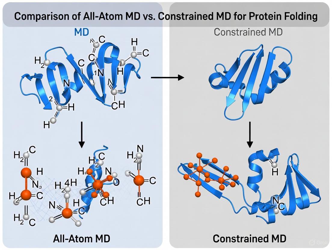
Understanding how a protein's amino acid sequence dictates its unique three-dimensional structure represents the central challenge of the "protein folding problem." This process is fundamental to biology, as a protein's specific structure determines its function. Computational methods have emerged as indispensable tools for probing folding mechanisms at atomic detail, complementing experimental approaches. Among these, all-atom Molecular Dynamics (MD) and constrained MD have become prominent strategies, each with distinct trade-offs between computational cost, sampling efficiency, and biological realism [1] [2]. All-atom MD simulations model every atom in the system using Cartesian coordinates and face significant timescale limitations due to the need for small integration time steps (typically 1-2 femtoseconds). In contrast, constrained MD methods, also known as torsion-angle MD, reduce the number of degrees of freedom by fixing bond lengths and angles, treating only torsional angles as flexible [1]. This fundamental difference in approach leads to dramatic variations in performance, sampling capabilities, and applicability to different protein systems, making a direct comparison essential for researchers choosing the appropriate tool for their folding investigations.

Methodological Comparison: All-Atom MD vs. Constrained MD

Fundamental Principles and Dynamic Models

The core distinction between these methods lies in their treatment of molecular flexibility and their coordinate systems.

• All-Atom MD operates in the Cartesian coordinate space, where every atom moves independently. This provides maximum flexibility but necessitates very small time steps to integrate the high-frequency vibrations of covalent bonds. The equations of motion are relatively simple but must be solved for a vast number of particles [2].

• Constrained MD operates in internal coordinate space, specifically using torsional angles as the primary degrees of freedom. Bond lengths and bond angles are constrained using rigid bodies or clusters, effectively eliminating the fastest vibrational modes. This reduces the number of degrees of freedom by approximately an order of magnitude. However, the equations of motion become more complex, requiring the inversion of a dense mass matrix. Algorithms like the Newton-Euler Inverse Mass Operator (NEIMO) and its generalized form (GNEIMO) solve these equations with O(N) computational cost, making them practical for proteins [1].

Quantitative Performance Metrics

The following table summarizes the key performance characteristics of both methods, highlighting their comparative advantages.

Table 1: Performance Comparison of All-Atom MD and Constrained MD for Protein Folding

Feature	All-Atom MD	Constrained MD
Degrees of Freedom	~3N (N = number of atoms); Very high [1]	~Ntorsions; ~10x fewer than all-atom MD [1]
Integration Time Step	~1-2 femtoseconds (fs) [1]	~5 fs or larger [1]
Computational Scaling	Scales with number of atoms; efficient for small systems	O(N) with NEIMO algorithm; efficient for larger systems [1]
Enhanced Sampling (Replica Exchange)	Requires many replicas (~√Ndof); high cost [1]	Requires ~3x fewer replicas due to fewer degrees of freedom [1]
Conformational Sampling	Can be limited by timescales; may get trapped in local minima	Wider conformational search; enhanced enrichment of near-native structures [1] [3]
Typical Applications	Folding of very small peptides/proteins; detailed mechanistic studies	Folding of small proteins (e.g., Trp-cage, WW domain); hierarchical folding studies [1] [4]

Experimental Protocols and Workflows

Standard Protocol for Constrained MD Folding Simulations

The following workflow outlines a typical protocol for employing constrained MD in protein folding studies, as described in research on peptides like polyalanine and Trp-cage [1].

Step-by-Step Protocol:

• System Preparation: Begin with the protein's amino acid sequence in an extended conformation. This provides an unbiased starting point far from the native state [1].
• Energy Minimization: Perform an initial energy minimization, for example using a conjugate gradient method, to relieve any steric clashes or unrealistic geometries from the initial structure. A typical convergence criterion is a force gradient below 10⁻² kcal/mol/Å [1].
• Simulation Setup:
  • Force Field & Solvation: Use an empirical force field (e.g., AMBER parm99) with an implicit solvation model such as Generalized-Born Surface Area (GB/SA). This avoids the computational expense of explicit water molecules. Parameters include an interior dielectric of 1.75, exterior dielectric of 78.3 for water, and a nonpolar surface tension term with a 1.4 Å solvent probe radius [1].
  • Replica Exchange: Set up a Replica Exchange (REMD) simulation. For constrained MD, 6-8 replicas spanning a temperature range (e.g., 325K to 500K) are often sufficient due to the reduced number of degrees of freedom. Exchanges between neighboring temperatures are attempted every 2 ps [1].
  • Constrained MD Engine: Configure the constrained MD parameters. This includes using an integrator like Lobatto with a 5 fs time step, which is 2-5 times larger than typical all-atom MD steps. Apply a cutoff (e.g., 20 Å) for non-bonded interactions with a smooth switching function [1].
• Production Simulation: Run the GNEIMO simulation for each replica. A total simulation time of up to 20 ns per replica has been used to fold small proteins like the 20-residue Trp-cage [1].
• Hierarchical Refinement (Optional): To enhance sampling of the native basin, a "freeze and thaw" protocol can be implemented. This involves identifying partially formed secondary structure elements (e.g., helical regions) from the initial all-torsion trajectory, freezing them into rigid clusters, and then resampling only the torsional degrees of freedom connecting these clusters [1] [3].
• Trajectory Analysis:
  • Structural Metrics: Calculate the Root Mean Square Deviation (RMSD) of sampled structures from the known native structure to assess proximity to the native state.
  • Secondary Structure: Monitor the formation of secondary structure. For example, a residue can be considered helical if its backbone dihedrals (φ, ψ) are within 20° of ideal α-helical angles (-57°, -47°) [1].
  • Conformational Clustering: Use algorithms like K-means clustering on the trajectory snapshots to group structurally similar conformations. The population percentage of each cluster indicates the relative stability of different states [1].
  • Principal Component Analysis (PCA): Project the trajectory onto the first two principal components derived from the Cα atom coordinates to visualize the explored conformational landscape and the density of states [1].

Protocol for All-Atom Discrete MD (DMD) Simulations

As a point of comparison, all-atom Discrete Molecular Dynamics (DMD) offers an alternative, rapid-sampling approach. The workflow for this method is distinct [4].

Key Methodological Details for DMD:

• Protein Model: Employs a united-atom model where heavy atoms and polar hydrogens are explicitly represented [4].
• Force Field: Uses a transferable force field that combines:
  • Van der Waals potentials to model atomic packing.
  • Lazaridis-Karplus effective energy to model solvation effects.
  • Explicit, environment-dependent hydrogen bond interactions. A key feature is that the desolvation penalty for a backbone carbonyl oxygen is reduced when it is hydrogen-bonded, making buried H-bonds (~3.1 kcal/mol) stronger than solvent-exposed ones (~1.0-2.0 kcal/mol), in agreement with experimental mutagenesis studies [4].
• Sampling and Analysis: Simulations also use the Replica Exchange (REXDMD) protocol starting from extended chains. The Weighted Histogram Analysis Method (WHAM) is then applied to the simulation data to compute the density of states and reconstruct folding free energy landscapes and thermodynamics [4].

The Scientist's Toolkit: Essential Research Reagents and Solutions

Successful execution of computational folding studies relies on a suite of software tools, force fields, and analysis utilities. The following table details key "research reagents" for the field.

Table 2: Essential Reagents for Computational Protein Folding Studies

Reagent / Resource	Type	Primary Function	Example Use Case
GNEIMO Simulation Package [1]	Software Algorithm	Performs constrained MD simulations with "freeze and thaw" capabilities.	Folding of small proteins with hierarchical clustering.
AMBER parm99/ff14SB [1]	Force Field	Defines potential energy terms for all-atom and constrained MD.	Providing empirical energy parameters for proteins.
CHARMM36/27 [5]	Force Field	Alternative force field for all-atom MD simulations.	Simulating folded proteins, membranes, and nucleic acids.
GB/SA Implicit Solvent [1]	Solvation Model	Approximates solvent effects without explicit water molecules.	Reducing computational cost in folding simulations.
Replica Exchange Method [1] [4]	Sampling Algorithm	Enhances conformational sampling by running parallel simulations at different temperatures.	Overcoming kinetic traps in both all-atom and constrained MD.
CUFIX Corrections [5]	Force Field Parameters	Refined non-bonded parameters to prevent artificial aggregation in MD.	Improving realism in simulations of DNA, lipids, and proteins.
Discrete MD (DMD) [4]	Simulation Engine	Rapid collision-driven dynamics with a united-atom model.	Ab initio folding of small proteins (e.g., Trp-cage, Villin).
Weighted Histogram Analysis Method (WHAM) [4]	Analysis Tool	Computes density of states and free energies from replica exchange simulations.	Determining folding thermodynamics (e.g., ΔG, melting temperature).

The choice between all-atom MD and constrained MD for tackling the protein folding problem is not a matter of identifying a superior method, but rather of selecting the right tool for the specific research objective. Constrained MD, with its reduced degrees of freedom and capacity for larger time steps, offers a computationally efficient path for rapidly sampling the conformational landscape and enriching for native-like structures of small proteins. Its unique ability to implement hierarchical "freeze and thaw" schemes provides a computational analog to the zipping-and-assembly folding model [1] [3]. In contrast, all-atom MD remains the gold standard for atomic-level detail and can yield quantitatively accurate folding rates and free energies when very long timescales are accessible, despite its higher computational cost [2]. Emerging methods like all-atom DMD with environment-aware force fields offer a promising middle ground, providing enhanced sampling while retaining an all-atom representation [4]. As force fields continue to be refined [2] [5] and computational power grows, the integration of these approaches—using constrained or coarse-grained methods for broad exploration followed by all-atom refinement—presents a powerful strategy to fully unravel the complexities of protein folding.

Molecular dynamics (MD) simulation is a cornerstone technique in computational chemistry and structural biology, enabling scientists to observe the time-evolving physical movements of atoms and molecules. Among the various approaches, All-Atom Molecular Dynamics (All-Atom MD) stands as the most detailed method, explicitly representing every atom in a system to provide unparalleled resolution of molecular interactions. This guide objectively compares All-Atom MD with an alternative methodology—Constrained MD—focusing on their application in protein folding research, a critical area for understanding cellular function and advancing drug development.

The fundamental distinction lies in their treatment of molecular degrees of freedom. All-Atom MD simulations model systems in full Cartesian space, accounting for every atomic vibration and movement, which comes at an extreme computational cost [6]. In contrast, Constrained MD employs a reduced representation, typically treating molecules as interconnected rigid bodies with flexible torsional hinges, thereby decreasing the number of degrees of freedom by an order of magnitude [1]. This comparison examines the performance trade-offs between these approaches, supported by experimental data and methodological details.

Methodological Comparison: All-Atom vs. Constrained MD

The core differences between All-Atom and Constrained MD simulations arise from their underlying molecular models and the integration techniques used to solve the equations of motion.

Table 1: Fundamental Methodological Differences

Feature	All-Atom MD	Constrained MD
Molecular Model	All atoms represented in Cartesian space [6]	Atoms grouped into rigid clusters connected by flexible torsional hinges [1]
Degrees of Freedom	3N (where N is the number of atoms) [6]	~N/10 (significantly reduced) [1]
High-Frequency Motions	Explicitly simulated (bond vibrations, angle deformations)	Mathematically constrained (fixed bond lengths and angles) [1]
Equation Solver	Cartesian dynamics (e.g., Verlet algorithm)	Internal coordinate dynamics (e.g., NEIMO algorithm) [1]
Typical Time Step	~1-2 femtoseconds (fs) [1]	~5 femtoseconds (fs) or larger [1]

A key advancement in Constrained MD is the Generalized Newton-Euler Inverse Mass Operator (GNEIMO) method. This algorithm, derived from Spatial Operator Algebra, solves the coupled equations of motion in internal coordinates with computational complexity that scales linearly with the number of degrees of freedom (O(N)), making it practical for large protein systems [1]. Furthermore, the GNEIMO framework enables hierarchical "freeze and thaw" clustering schemes, where secondary structure elements like alpha-helices can be temporarily treated as rigid bodies while sampling only the connecting torsions, potentially accelerating convergence to native folds [1].

Experimental Protocols for Protein Folding Studies

Standard All-Atom MD Folding Protocol

To ensure meaningful comparisons, researchers typically follow a standardized protocol when applying All-Atom MD to protein folding:

• Initial System Preparation: The simulation begins with an extended conformation of the peptide or protein sequence [1].
• Energy Minimization: The initial structure undergoes conjugate gradient minimization to remove steric clashes and achieve a stable starting configuration, typically with a convergence criterion of 10⁻² kcal/mol/Å in force gradient [1].
• Solvation Model: Simulations employ either explicit solvent molecules or implicit solvation models. The Generalized-Born/Surface Area (GB/SA) model is common, with an interior dielectric of 1.75 for the solute and exterior dielectric of 78.3 for water [1].
• Force Field Application: Modern protein force fields (e.g., AMBER, CHARMM) are applied, parameterized on quantum-chemical calculations and experimental data [6].
• Dynamics Simulation: Numerical integration of Newton's equations of motion is performed with a small time step (1-2 fs) to accurately resolve atomic vibrations. Non-bonded forces are often smoothly switched off at a cutoff radius (e.g., 20Å) [1].
• Enhanced Sampling (Optional): To overcome timescale limitations, techniques like replica exchange molecular dynamics (REMD) are often employed, running multiple simulations at different temperatures to facilitate escape from local energy minima [1].

Constrained MD Replica Exchange Protocol

The constrained MD approach modifies this protocol to leverage its computational advantages:

• Initialization and Minimization: Steps 1 and 2 are identical to the All-Atom protocol [1].
• Constrained Dynamics Setup: The molecule is partitioned into rigid clusters and flexible torsional hinges. The GNEIMO method is initialized with these constraints [1].
• Solvation and Force Field: Similar GB/SA implicit solvation is used, along with compatible force fields like parm99 [1].
• Dynamics Integration: The simulation uses an internal coordinate Lobatto integrator with a larger time step (e.g., 5 fs) due to the eliminated high-frequency vibrations [1].
• Replica Exchange Enhancement: Replica Exchange is coupled with Constrained MD. A key advantage is that the number of replicas required is reduced (approximately by a factor of three) because it depends on the square root of the number of degrees of freedom, which is already much lower in Constrained MD [1]. A typical setup might use 8 replicas across a temperature range of 325K to 500K [1].

Figure 1: Comparative Workflow for Protein Folding Simulations

Performance Comparison and Experimental Data

Direct comparative studies and performance benchmarks reveal the strengths and limitations of each method for specific research applications.

Computational Efficiency and Sampling Effectiveness

Table 2: Performance Comparison on Protein Folding Tasks

Performance Metric	All-Atom MD	Constrained MD	Experimental Context
Time Step	~1-2 fs [1]	≥5 fs [1]	Stable integration step size
Computational Cost	Extremely high [6]	Order of magnitude decrease [1]	For equivalent simulation time
Replica Exchange Efficiency	Requires more replicas [1]	Requires ~3x fewer replicas [1]	Number of replicas needed for efficient sampling
Conformational Search Breadth	Standard search	Wider conformational search [1]	Measured by diversity of sampled structures
Native-State Enrichment	Standard enrichment	Increased enrichment of near-native structures [1]	Fraction of sampled structures close to known native fold
Applicability to Timescales	Nanoseconds to milliseconds [6]	Enables longer effective timescales [1]	Biologically relevant processes

A study focusing on small proteins like the α-helical polyalanine and the mixed-motif Trp-cage protein demonstrated that Constrained MD replica exchange simulations exhibited a wider conformational search than All-Atom MD, with increased enrichment of near-native structures [1]. Furthermore, "hierarchical" Constrained MD simulations, where partially formed helical regions were frozen, showed even better sampling of native structures, aligning with zipping-and-assembly folding models [1].

Accuracy in Predicting Structural Landscapes

Recent machine-learned Coarse-Grained (CG) models, which also reduce degrees of freedom, demonstrate the predictive potential of non-all-atom approaches. One such universal CG model was shown to successfully predict metastable states of folded, unfolded, and intermediate structures for various small proteins (e.g., chignolin, TRP-cage, villin headpiece), achieving results comparable to All-Atom MD references but at a fraction of the computational cost [6]. However, the study noted that while the CG model correctly identified native state basins, the relative free energy differences between metastable states did not always exactly match the All-Atom MD reference, particularly for complex proteins like the beta–beta–alpha fold (BBA) which contains both helical and β-sheet motifs [6]. This highlights a common trade-off: reduced models gain efficiency but can sacrifice quantitative energetic precision.

Figure 2: Method Selection Guide for Research Objectives

The Scientist's Toolkit: Essential Research Reagents

Successful implementation of these simulation methods requires a suite of specialized software, force fields, and computational resources.

Table 3: Key Research Reagents for MD Simulations

Reagent / Tool	Type	Primary Function	Example Applications
AMBER (parm99)	Force Field [1]	Defines potential energy terms (bonds, angles, torsions, electrostatics, van der Waals) for proteins and nucleic acids.	Provides energy parameters for folding simulations with All-Atom or Constrained MD [1].
GB/SA (OBC Model)	Implicit Solvation Model [1]	Approximates solvent effects without explicit water molecules, significantly reducing computational cost.	Used in protein folding studies to model aqueous environment [1].
GNEIMO Algorithm	Constrained MD Solver [1]	Efficiently solves equations of motion in internal coordinates with O(N) computational scaling.	Enables all-torsion and hierarchical clustering MD simulations [1].
Replica Exchange MD	Enhanced Sampling Algorithm [1]	Facilitates escape from local energy minima by running parallel simulations at different temperatures.	Improves conformational sampling in both All-Atom and Constrained MD protein folding studies [1].
Machine-Learned Coarse-Grained (CG) Force Fields	Neural Network Potential [6]	Learns effective physical interactions between CG degrees of freedom from all-atom data.	Transferable simulation of protein dynamics and folding for new sequences [6].

The choice between All-Atom MD and Constrained MD is not a matter of which method is universally superior, but which is optimal for a specific research question. All-Atom MD remains the gold standard for capturing full atomic detail and providing quantitative energetic information, making it indispensable for studying atomic-level mechanisms and validating reduced models. Its primary limitation is computational expense, restricting accessible timescales and system sizes.

Constrained MD offers a powerful alternative for efficiently exploring protein folding pathways and enriching samples with native-like structures, particularly when enhanced with replica exchange and hierarchical clustering schemes. Its ability to simulate longer effective timescales makes it valuable for initial folding studies and larger systems.

The field is increasingly witnessing a paradigm where these methods are not just alternatives but complementary tools. All-Atom simulations provide the foundational data for developing and validating more efficient coarse-grained and machine-learned models, which in turn can explore biological questions at scales previously unreachable. This synergistic combination, leveraging the detail of all-atom representations and the scale of reduced models, represents the future of computational molecular biology.

Molecular dynamics (MD) simulation is a powerful computational microscope, enabling researchers to observe the intricate structural dynamics of proteins at atomic resolution. However, a significant challenge in simulating protein folding is the massive computational cost of all-atom Cartesian MD, as folding processes often occur on timescales of microseconds or longer, which are prohibitively expensive to simulate with conventional methods [1]. The fundamental issue lies in the numerous high-frequency vibrations in bond lengths and angles, which limit the integration time step to typically 1-2 femtoseconds, requiring billions of steps to reach biologically relevant timescales [7].

Constrained MD presents an alternative approach that addresses this sampling bottleneck through a reduction in the system's degrees of freedom. By imposing holonomic constraints on bond lengths and bond angles, the molecule is modeled as a collection of rigid bodies connected by flexible torsional hinges [1]. This review provides a comprehensive comparison between all-atom MD and constrained MD methodologies, focusing on their application to protein folding research, with supporting experimental data and detailed protocols.

Methodological Fundamentals: A Tale of Two Approaches

All-Atom Molecular Dynamics

In all-atom Cartesian MD, the motion of every atom in the system is simulated by numerically solving Newton's equations of motion. Each atom is treated as an independent entity with its own coordinates and velocities, resulting in approximately three degrees of freedom per atom. The forces acting on each atom are derived from empirical potential energy functions that describe bonded interactions (bonds, angles, dihedrals) and non-bonded interactions (van der Waals, electrostatic) [8]. While this approach provides the most detailed representation of atomic movements, it becomes computationally prohibitive for studying folding events that exceed microsecond timescales [1].

Constrained Molecular Dynamics

Constrained MD, also known as internal coordinate MD or torsion angle MD, fundamentally reduces the system's complexity by fixing the covalent geometry within rigid clusters of atoms. The number of degrees of freedom in constrained MD models is approximately one order of magnitude smaller than in all-atom models [1]. This reduction enables two significant advantages: (1) the elimination of high-frequency vibrations permits larger integration time steps (typically 4-5 fs), and (2) the decreased number of degrees of freedom reduces computational complexity per time step.

The Generalized Newton-Euler Inverse Mass Operator (GNEIMO) method implements constrained MD using the Spatial Operator Algebra mathematical framework, solving the equations of motion with O(N) computational cost compared to conventional O(N³) methods, where N represents the number of torsional degrees of freedom [1]. This algorithmic efficiency makes constrained MD particularly suitable for studying larger protein systems.

Figure 1: Methodological comparison between all-atom MD and constrained MD approaches, highlighting fundamental differences in degrees of freedom (DOFs) and their computational implications.

Quantitative Performance Comparison

Computational Efficiency Metrics

Multiple studies have directly compared the performance of constrained and all-atom MD simulations for protein folding applications. The data reveals significant advantages in computational efficiency for constrained methods while maintaining structural accuracy.

Table 1: Computational efficiency comparison between all-atom MD and constrained MD

Parameter	All-Atom MD	Constrained MD	Improvement Factor
Degrees of Freedom	~3N (Cartesian coordinates)	~N (torsional angles)	~3× reduction [1]
Time Step	1-2 fs	4-5 fs	2-5× larger [1]
Replica Exchange Replicas	Proportional to √(3N)	Proportional to √N	~3× fewer replicas [1]
Sampling Enhancement	Baseline	Wider conformational search [1]	Significant
Near-Native Structure Enrichment	Baseline	Increased enrichment [1]	Significant

Sampling Effectiveness in Protein Folding

The true value of any enhanced sampling method lies in its ability to efficiently explore the conformational landscape and identify biologically relevant states. Constrained MD coupled with replica exchange has demonstrated remarkable effectiveness in folding small proteins with various secondary structural motifs.

Table 2: Sampling performance of constrained MD replica exchange for various protein systems

Protein System	Structural Motif	Simulation Details	Key Findings
Polyalanine (20-mer)	α-helix	All-torsion constrained MD, GB/SA solvent, 300K [1]	Successfully folded with stable helicity; did not require elevated temperatures
WALP16	Transmembrane α-helix	All-torsion constrained MD, GB/SA with dielectric 40, 300K [1]	Correct folding in membrane-mimetic environment
1E0Q	β-turn	All-torsion constrained MD, GB/SA solvent [1]	Native-like structure formation
Trp-cage	Mixed motif	Hierarchical constrained MD, GB/SA solvent [1]	Better sampling of near-native structures than all-torsion MD

The hierarchical variation of constrained MD, where partially formed secondary structure regions are treated as rigid clusters while sampling only the connecting torsions, has shown particular promise. For the Trp-cage protein, this approach demonstrated superior sampling of near-native structures compared to all-torsion constrained MD, supporting the zipping-and-assembly folding model proposed by Dill and coworkers [1].

Experimental Protocols and Methodologies

Constrained MD with Replica Exchange Protocol

The following detailed methodology has been successfully employed for protein folding studies using constrained MD:

System Preparation:

• Start from an extended conformation of the peptide/protein sequence
• Perform conjugate gradient minimization with convergence criterion of 10⁻² kcal/mol/Å in force gradient [1]

Simulation Parameters:

• Force Field: parm99 (part of AMBER99 force field) [1]
• Solvation: Implicit Generalized-Born Surface Area (GB/SA) with OBC model [1]
• Dielectric Constants: Interior = 1.75, Exterior = 78.3 (water) or 40.0 (membrane) [1]
• Non-bond Cutoff: 20Å with smooth switching [1]
• Integrator: Lobatto integrator with 5 fs time step [1]

Replica Exchange Configuration:

• Temperature Range: 325K to 500K in steps of 25K (6-8 replicas total) [1]
• Exchange Attempt Frequency: Every 2ps [1]
• Simulation Duration: Up to 20ns per replica [1]
• Replica Exchange Acceptance: Metropolis criterion based on Boltzmann factors [9]

Hierarchical Clustering Schemes:

• Identify partially formed secondary structure elements during simulation
• Freeze these regions as rigid clusters
• Sample only torsional degrees of freedom connecting these clusters
• Enable "freeze and thaw" dynamics based on structural stability [1]

Analysis Methods

Principal Component Analysis (PCA):

• Construct covariance matrices of Cα atom coordinates from trajectory snapshots
• Project simulation trajectories onto the first two principal components
• Generate density maps to visualize population distributions [1]

Cluster Analysis:

• Apply K-means clustering algorithm to group structurally similar conformations
• Generate representative structures by averaging 1000 snapshots from each cluster
• Calculate population percentages as fraction of conformations in each cluster [1]

Native Structure Metrics:

• For α-helical structures: Residue considered helical if backbone torsional angles within 20° of ideal α-helical angles (φ = -57°, ψ = -47°) [1]
• helicity defined as fraction of total residues in helical conformation [1]

Table 3: Key computational tools and resources for constrained MD simulations

Resource Category	Specific Tools/Resources	Function and Application
Constrained MD Software	GNEIMO [1]	Implements constrained MD with O(N) computational scaling
All-Atom MD Packages	CHARMM, AMBER, NAMD [1]	Traditional Cartesian MD simulation with explicit solvent capabilities
Enhanced Sampling Methods	Replica Exchange [1] [9]	Enhanced conformational sampling through temperature parallelism
Implicit Solvent Models	GB/SA OBC model [1]	Efficient solvation treatment without explicit water molecules
Force Fields	AMBER parm99 [1], CHARMM22* [10]	Empirical potential energy functions for biomolecular simulations
Structure Databases	Protein Data Bank (PDB) [11] [8]	Source of experimental protein structures for simulation initial conditions
Analysis Tools	Principal Component Analysis, K-means Clustering [1]	Extraction of essential dynamics and conformational clustering
Validation Datasets	mdCATH [10]	Large-scale MD dataset for validation and comparison of simulation methods

Integration with Advanced Sampling and Emerging Methods

Constrained MD represents one approach within a broader ecosystem of enhanced sampling techniques. Replica exchange methods have proven particularly compatible with constrained MD, as the reduced number of degrees of freedom decreases the number of replicas required for efficient sampling by approximately a factor of three [1]. This synergy significantly enhances the computational advantages of constrained MD.

Recent advancements in machine learning interatomic potentials (MLIPs) and artificial intelligence are creating new opportunities for both all-atom and constrained MD approaches [10] [8]. These technologies promise to bridge the gap between computational efficiency and physical accuracy, potentially revolutionizing protein folding simulations in the coming years.

The mdCATH dataset, comprising over 62 milliseconds of accumulated all-atom simulation time across 5,398 protein domains, provides a valuable resource for validating constrained MD methods and developing next-generation potentials [10]. Such large-scale datasets enable systematic comparison of simulation methods across diverse protein architectures.

Constrained MD offers a computationally efficient alternative to all-atom MD for protein folding studies, particularly when combined with enhanced sampling techniques like replica exchange. The methodological approach of reducing degrees of freedom through fixed bond geometry enables longer time steps and decreased computational complexity, resulting in significantly enhanced conformational sampling for a given computational budget.

The hierarchical implementation of constrained MD, which allows dynamic "freezing and thawing" of secondary structure elements, provides particularly promising results that align with modern understanding of protein folding pathways. This approach demonstrates increased enrichment of near-native structures and wider exploration of the conformational landscape compared to all-atom methods.

While all-atom MD remains the gold standard for detailed atomic-level simulation, constrained MD establishes itself as a valuable tool for rapid exploration of folding pathways and identification of native-like states, especially for small to medium-sized proteins. The choice between these methodologies should be guided by research objectives, computational resources, and the specific balance required between atomic detail and sampling efficiency.

The process by which a protein folds from a linear amino acid chain into a functional three-dimensional structure is a fundamental problem in computational biophysics. This process occurs on timescales ranging from microseconds to minutes, yet the conformational space available to even a small protein is astronomically large. This dichotomy is the heart of Levinthal's paradox, which posits that a random, exhaustive search of all possible conformations would take billions of years, far longer than the observed folding times [12]. This paradox has driven the development of the free energy landscape theory, where folding is envisioned not as a random search but as a funneled process that directs the protein toward its native state, the global free energy minimum [12] [13]. Molecular dynamics (MD) simulations provide a powerful tool for studying these landscapes. This guide offers a critical comparison between all-atom MD and constrained MD methods, evaluating their performance in elucidating protein folding mechanisms for a research audience.

Theoretical Framework: Resolving the Paradox

The Free Energy Landscape and Folding Timescales

Levinthal's paradox highlights the impossibility of a protein folding via a random conformational search. For a 100-residue protein, with at least two conformations per residue, there are at least 2¹⁰⁰ (~10³⁰) possibilities. Sampling each at a picosecond rate would take ~10¹⁰ years [12]. The resolution lies in the fact that the search is not random; the amino acid sequence encodes a funneled energy landscape [13]. In this "new view" of folding, the landscape is not rugged but smooth and biased toward the native state, guiding the protein through a subset of pathways and enabling folding on biologically feasible timescales (milliseconds to minutes) [12] [13]. The folding process can be thermodynamically controlled, where the native state is the global free energy minimum, and proteins reliably find it without needing to sample all possibilities [12].

The Role of Molecular Dynamics Simulations

Molecular Dynamics simulations computationally simulate the physical movements of atoms and molecules over time. All-atom MD explicitly models every atom in the system, integrating Newton's equations of motion to produce atomic trajectories [14]. This allows researchers to directly observe the time evolution of molecular structures and explore conformational ensembles [14]. The accuracy of traditional MD, however, is limited by the computational cost of calculating all interatomic forces and the need for extremely small timesteps (femtoseconds), which severely restricts the accessible timescales for biologically relevant processes [14].

Table 1: Key Concepts in Protein Folding

Concept	Description	Implication for MD Simulation
Levinthal's Paradox	The apparent contradiction between the vast conformational space and observed fast folding times [12].	Justifies the need for enhanced sampling methods beyond brute-force simulation.
Free Energy Landscape	A theoretical model depicting protein conformations on a surface biased toward the native state [13].	The central object that MD simulations aim to characterize and understand.
Folding Funnel	A specific type of landscape where the native state is a deep, broad minimum, making folding efficient and reliable [13].	A funneled landscape reduces the computational burden for all-atom MD to simulate folding.
Thermodynamic Control	Folding is directed to the global free energy minimum because it is the most stable state [12].	Validates the goal of simulations to find the global minimum.

Methodologies: All-Atom MD vs. Constrained and Enhanced MD

This section details the core computational protocols for the methods discussed in this guide.

All-Atom Molecular Dynamics

Objective: To simulate the full, unconstrained dynamics of a biomolecular system at atomic resolution for the longest possible timescale.

Detailed Protocol:

• System Preparation: The protein structure is placed in a simulation box solvated with explicit water molecules (e.g., TIP3P model). The system is neutralized by adding ions (e.g., Na⁺ and Cl⁻) to a physiological concentration (e.g., 0.150 M) [10].
• Force Field Parameterization: All atoms are assigned parameters using a classical force field (e.g., CHARMM22*). These force fields define the potential energy function, including bonded terms (bonds, angles, dihedrals) and non-bonded terms (van der Waals and electrostatic interactions) [10].
• Equilibration: The system undergoes a multi-stage energy minimization and equilibration process. This is typically done in the NPT ensemble (constant Number of particles, Pressure, and Temperature) at 1 atm and 300 K, often with harmonic restraints on protein heavy atoms that are gradually released [10].
• Production Simulation: The unrestrained simulation is run, usually in the NVT (constant Number, Volume, Temperature) ensemble using a thermostat (e.g., Langevin thermostat). Long-range electrostatic forces are handled with particle-mesh Ewald (PME) summation. A timestep of 2-4 fs is used, often enabled by hydrogen mass repartitioning [10].
• Data Analysis: Trajectories (atomic coordinates saved every 1-100 ps) are analyzed for properties like Root-Mean-Square Deviation (RMSD), Root-Mean-Square Fluctuation (RMSF), and secondary structure evolution to study folding pathways and stability.

Enhanced Sampling Methods (Constrained MD)

Objective: To accelerate the sampling of rare events, such as protein folding or ligand unbinding, that occur on timescales beyond the reach of standard all-atom MD.

Detailed Protocol (Metadynamics):

• Collective Variable (CV) Selection: Identify a small number of CVs (e.g., root-mean-square deviation (RMSD) from the native state, radius of gyration, number of native contacts) that describe the slow degrees of freedom of the folding process [14].
• Bias Potential Deployment: A history-dependent bias potential, typically composed of repulsive Gaussians, is added to the system's Hamiltonian during the simulation [14].
• Filling Energy Wells: This bias potential is periodically added along the chosen CVs, discouraging the system from revisiting already sampled conformations. This effectively "fills up" the free energy wells, pushing the system to explore new regions of the conformational landscape [14].
• Free Energy Surface Construction: Once the simulation converges, the accumulated bias potential provides a direct estimate of the underlying free energy surface as a function of the selected CVs, revealing the relative stability of folded, unfolded, and intermediate states [14].

Performance Comparison

This section provides a quantitative and qualitative comparison of all-atom MD and enhanced/constrained MD methods, focusing on their utility in protein folding studies.

Table 2: Comparative Analysis of MD Simulation Approaches for Protein Folding

Feature	All-Atom MD	Constrained/Enhanced MD (e.g., Metadynamics)
Spatial Resolution	All-atom, high resolution [14].	All-atom, but dynamics are biased by collective variables.
Accessible Timescales	Nanoseconds to microseconds, rarely milliseconds [14].	Effectively microseconds to seconds and beyond for specific events [14].
Computational Cost	Extremely high; scales poorly with system size [14].	High, but more efficient per unit of conformational space explored.
Handling of Levinthal's Paradox	Directly simulates physical pathways but may not reach folded state within feasible time for some proteins.	Actively drives the system over energy barriers to find minima.
Primary Output	Time-resolved trajectory of all atomic positions [14].	Free energy landscape and preferred pathways as a function of collective variables [14].
Key Limitation	Computationally limited timescales may miss slow folding events [15].	Choice of collective variables introduces bias; may miss important pathways not described by the CVs.
Ideal Use Case	Studying local dynamics, folding of small fast-folding proteins, and protein-ligand interactions [16].	Mapping free energy landscapes, sampling rare events like large-scale conformational changes and unbinding [14].

Performance Metrics and Experimental Data

The comparison between these methods is best illustrated with specific examples from the literature. A landmark study on the mdCATH dataset, which comprises over 62 ms of accumulated all-atom MD simulation time across 5,398 protein domains, demonstrates the raw power and limitations of standard MD. While this vast dataset captures unfolding thermodynamics and kinetics at multiple temperatures, it also underscores the computational expense required to study folding, even for small domains [10].

In contrast, enhanced methods like Metadynamics are designed to overcome these timescale barriers. For instance, the BioMD generative model, which incorporates principles from enhanced sampling, successfully generated ligand unbinding pathways for 97.1% of protein-ligand systems in a benchmark, a task prohibitively expensive for standard all-atom MD [14]. Furthermore, Gaussian accelerated MD (GaMD), a different enhanced sampling technique, has been used to capture slow events like proline isomerization in intrinsically disordered proteins (IDPs), generating conformational ensembles that align well with experimental circular dichroism data [15].

Table 3: Experimentally Validated Outcomes from Different MD Approaches

Method	System Studied	Key Performance Result	Experimental Validation
All-Atom MD (mdCATH)	5,398 diverse protein domains [10].	Generated over 62 ms of simulation data; captured unfolding kinetics at multiple temperatures.	Provides a benchmark dataset for validating other methods and force fields [10].
AI/Enhanced Sampling (BioMD)	Protein-ligand unbinding [14].	Generated realistic unbinding paths for 97.1% of test systems.	Demonstrated high physical plausibility and low reconstruction error on benchmark datasets [14].
Gaussian Accelerated MD	ArkA, a proline-rich IDP [15].	Captured proline isomerization, leading to a more compact ensemble.	Conformational ensemble aligned with in-vitro circular dichroism data [15].

The Scientist's Toolkit: Essential Research Reagents and Solutions

Table 4: Key Computational Tools and Resources for Protein Folding Simulations

Item	Function	Example
Force Fields	Define the potential energy function and parameters for the simulated atoms.	CHARMM22* [10], AMBER, GROMOS.
Simulation Software	Software engines that perform the numerical integration of the equations of motion.	ACEMD [10], GROMACS, NAMD, OpenMM.
Enhanced Sampling Plugins	Implement algorithms like Metadynamics to accelerate rare events.	PLUMED.
Trajectory Analysis Tools	Libraries for analyzing simulation outputs (RMSD, RMSF, free energy, etc.).	HTMD [10], MDTraj, VMD.
Benchmark Datasets	Provide large-scale, standardized simulation data for method development and validation.	mdCATH [10], MISATO [14].
AI-Generative Models	Machine learning alternatives to physics-based MD for generating trajectories or ensembles.	BioMD [14], AlphaFold 3 (for complexes) [14].

Conceptual Workflows and Signaling Pathways

The following diagrams illustrate the core logical relationships and computational workflows described in this guide.

Protein Folding Energy Landscape

Diagram Title: Protein Folding Energy Landscape

MD Simulation Decision Workflow

Diagram Title: MD Simulation Decision Workflow

Methodologies and Practical Applications in Biomedical Research

This guide provides an objective comparison of contemporary molecular dynamics (MD) simulation parameters, focusing on the performance of all-atom force fields and solvation models for protein folding research, contextualized within a broader comparison with constrained MD methods.

All-atom molecular dynamics (MD) simulates every atom in a system, using Cartesian coordinates and typically requiring small integration time steps (e.g., 2 femtoseconds). This approach offers high detail but is computationally expensive, limiting the timescales that can be practically simulated [1].

Constrained MD, also known as internal coordinate MD or torsion angle MD, offers an alternative. It treats the molecule as a collection of rigid bodies connected by flexible torsional hinges, fixing bond lengths and bond angles. This reduces the number of degrees of freedom by approximately an order of magnitude, allowing for larger time steps (e.g., 5 fs) and decreased computational cost. This method can enhance conformational sampling, particularly for protein folding studies [1].

Performance Benchmarking of All-Atom Force Fields

The accuracy of any all-atom MD simulation is fundamentally dependent on the force field. Recent benchmarks have evaluated force fields for their ability to model complex proteins that contain both structured domains and intrinsically disordered regions (IDRs).

Benchmarking Study on FUS Protein

A comprehensive 2023 study benchmarked nine modern force fields using the full-length Fused in sarcoma (FUS) protein, a biologically relevant system containing long IDRs. The performance was assessed against experimental data from dynamic light scattering for the radius of gyration (Rg). Key findings are summarized in the table below [17].

Table 1: Performance of All-Atom Force Fields for Structured and Disordered Proteins (FUS Protein Benchmark)

Force Field Combination	Water Model	Performance Summary	Key Experimental Validation
DES-Amber [17]	Modified TIP4P-D	Optimal for IDPs while maintaining stability of folded domains [17].	FUS Rg within experimental range [17].
a99SB-disp [17]	Modified TIP4P-D	Excellent for disordered regions; derived from ff99SB [17].	FUS Rg within experimental range [17].
CHARMM36m [17]	TIP3P	Good performance for IDPs; includes modifications to CHARMM36 for folded/disordered balance [17].	FUS Rg within experimental range [17].
ff99SB-ILDN/DISP [17]	TIP4P-D	Good for IDPs; may slightly destabilize some folded proteins [17].	FUS Rg within experimental range [17].
ff19SB [17]	OPC	Recommended modern AMBER force field; improved with OPC water [17].	Data consistent with expectations [17].
ff14SB [17]	TIP3P	Popular for folded proteins; tends to produce overly compact IDRs [17].	FUS Rg too compact vs. experiment [17].
CHARMM36 [17]	TIP3P	Conventional force field for folded proteins; IDRs too compact [17].	FUS Rg too compact vs. experiment [17].
ff99SB-ILDN [17]	TIP3P	Improved side-chain torsions; IDRs still too compact with TIP3P [17].	FUS Rg too compact vs. experiment [17].
ff03ws [17]	TIP4P/2005	Scaled water-protein interactions; accurate for short IDPs in crowded environments [17].	Not specifically mentioned in FUS benchmark [17].

Specialized Benchmarking for Collagen Systems

For specific protein families like collagen, specialized benchmarks are necessary. A 2025 study found that AMBER force fields (e.g., ff99SB) accurately reproduced collagen triple helix structure and dynamics compared to crystal structures, NMR data, and SAXS form factors. In contrast, CHARMM36 force fields systematically shifted backbone dihedrals, though this could be corrected by scaling specific CMAP terms [18].

Comparison of Implicit Solvation Models

Implicit solvation models, which approximate the solvent as a continuum, offer a computationally efficient alternative to explicit water molecules. They are crucial for achieving longer simulation timescales.

Table 2: Comparison of Implicit Solvation Methodologies

Solvation Method	Type	Computational Cost	Key Features & Applications
Generalized Born/Surface Area (GB/SA) [1]	Implicit	Low	Used with constrained MD to fold small proteins (e.g., polyalanine, Trp-cage); allows representation of water/membrane environments via dielectric constant [1].
Poisson-Boltzmann (PB) [19]	Implicit	High (Traditional)	Considered more accurate than GB but slower; requires solving equation on a large grid system [19].
Machine Learning PB [19]	Implicit	Low (after training)	Deep neural network predicts solvation forces; speed suitable for long trajectories; accuracy comparable to traditional PB [19].

Experimental Protocols for Key Studies

Protocol: All-Atom Force Field Benchmarking

The benchmark of force fields for the FUS protein followed a rigorous protocol to ensure a fair comparison [17]:

• System Preparation: The full-length FUS protein (526 residues) was simulated starting from extended or structured initial conditions.
• Simulation Parameters: Simulations were conducted on the Anton 2 supercomputer. Multiple independent simulations were run for 5 microseconds per force field to ensure statistical robustness.
• Analysis Metrics: The primary metric for comparison was the radius of gyration (Rg), benchmarked directly against experimental dynamic light scattering data. Additional metrics included solvent-accessible surface area (SASA), diffusion constants, and analysis of side-chain interactions.

Protocol: Constrained MD with Replica Exchange

A study on constrained MD for protein folding employed the following methodology [1]:

• Initialization: Simulations began with an extended conformation of the peptide/protein, minimized using conjugate gradient methods.
• Dynamics Model: The GNEIMO (Generalized Newton-Euler Inverse Mass Operator) constrained MD method was used, fixing bond lengths and angles and sampling only torsional degrees of freedom.
• Force Field & Solvation: The AMBER parm99 force field was used with an implicit GB/SA (OBC model) solvation.
• Enhanced Sampling: The Replica Exchange MD (REMD) method was integrated. For constrained MD, only 8 replicas in the 325K-500K range were needed (fewer than all-atom MD due to reduced degrees of freedom). Exchanges were attempted every 2ps, with total simulation times up to 20ns per replica.
• Hierarchical Clustering: Specific secondary structure elements (like pre-formed helices) could be "frozen" into rigid clusters, sampling only the torsions between them to accelerate convergence to the native state.

The Scientist's Toolkit: Essential Research Reagents & Software

Table 3: Key Computational Tools for All-Atom and Constrained MD Simulations

Tool Name	Category	Primary Function	Relevant Context
AMBER [1] [17]	Software Suite	MD simulation and force field development.	Includes ff14SB, ff19SB, ff99SB force fields; PBSA module for implicit solvation [1] [17].
CHARMM [1] [17]	Software Suite	MD simulation and force field development.	Includes CHARMM36, CHARMM36m force fields; PBEQ solver [1] [17].
GROMACS [18]	MD Engine	High-performance MD simulations.	Used for force field benchmarking (e.g., collagen studies) [18].
NAMD [17]	MD Engine	Parallel MD simulations.	Implemented best-performing force fields from Anton 2 benchmarks for community access [17].
GB/SA (OBC Model) [1]	Implicit Solvent	Approximates solvation effects.	Used in constrained MD folding studies to represent water or membrane environments [1].
TIP3P [17]	Water Model	3-point explicit water model.	Standard for many force fields (ff14SB, CHARMM36); can compact IDPs [17].
TIP4P-D/OPC [17]	Water Model	4-point explicit water models.	Improve description of IDPs; used with a99SB-disp, DES-Amber, ff19SB [17].
Replica Exchange MD [1]	Sampling Method	Enhanced conformational sampling.	Reduces the risk of being trapped in local energy minima; used in both all-atom and constrained MD [1].

The choice between all-atom and constrained MD, as well as the selection of specific force fields and solvation models, depends heavily on the specific research question and available computational resources.

• All-Atom MD remains the gold standard for its detailed physical representation. For systems containing intrinsically disordered regions, modern force fields like DES-Amber, a99SB-disp, and CHARMM36m coupled with four-point water models (e.g., TIP4P-D, OPC) have shown superior performance against experimental data.
• Constrained MD offers a computationally efficient alternative, particularly for initial folding studies and conformational sampling of small proteins. Its ability to use hierarchical clustering aligns with the "zipping-and-assembly" folding model and can accelerate the discovery of native-like structures [1].
• Solvation models are evolving, with machine-learning-assisted PB methods promising to combine the accuracy of traditional PB with the speed required for long-timescale simulations [19].

For researchers, this means that a careful consideration of the system's properties (folded vs. disordered), the desired observables, and the computational budget is essential for setting up successful and predictive MD simulations.

Molecular dynamics (MD) simulation is a cornerstone technique for studying protein folding, but its application is severely limited by the computational cost of simulating processes occurring on microsecond to millisecond timescales. All-atom Cartesian MD simulations require femtosecond integration time steps to resolve high-frequency bond vibrations, making folding simulations prohibitively expensive for many systems. Constrained MD methods address this fundamental limitation by reducing the number of degrees of freedom through the application of holonomic constraints, typically freezing bond lengths and angles while retaining torsional degrees of freedom. This approach allows for larger time steps (typically 4-5 fs) and more efficient conformational sampling by focusing computational resources on the slow, large-amplitude motions most relevant to protein folding. Research demonstrates that constrained MD methods not only accelerate simulations but can also enhance enrichment of near-native structures compared to all-atom MD, making them particularly valuable for protein structure prediction and refinement [1] [20].

The core principle behind constrained MD is the replacement of Cartesian atomic coordinates with internal coordinates as the primary degrees of freedom. This transforms the molecular system into a tree topology of rigid clusters connected by flexible torsional hinges, dramatically reducing the system's complexity. For a typical protein, constrained MD models operate with approximately one-tenth the degrees of freedom of all-atom models, leading to significant computational savings and enabling longer timescale simulations [1]. This guide provides a comprehensive comparison of constrained MD implementation strategies, with particular focus on clustering schemes and torsional dynamics algorithms for protein folding applications.

Methodological Approaches to Constrained MD

Algorithmic Foundations and Theoretical Frameworks

Constrained MD implementations vary in their mathematical formulation and coordinate systems, leading to distinct algorithmic families with different performance characteristics:

• Internal Coordinate MD (ICMD): These methods use bond, angle, and torsional (BAT) coordinates as the natural degrees of freedom instead of Cartesian coordinates. The Generalized Newton-Euler Inverse Mass Operator (GNEIMO) method is a leading implementation that uses Spatial Operator Algebra to solve the equations of motion with O(N) computational cost, making it practical for large proteins [20].

• Torsion Angle MD (TAMD): A specialized form of constrained ICMD that freezes all bond lengths and angles, leaving only torsional degrees of freedom. The molecule is represented as a collection of rigid bodies ("clusters") connected by flexible hinges, with the conformation uniquely specified by the values of all torsion angles [21] [22].

• Cartesian Constraint Algorithms: Methods like SHAKE, RATTLE, and WIGGLE implement constraints within Cartesian coordinate frameworks through iterative adjustment of atomic positions and/or velocities to satisfy bond length constraints. These algorithms provide moderate improvements (∼2 fs time steps) but don't achieve the same level of sampling efficiency as true internal coordinate methods [23] [24].

Table 1: Comparison of Constrained MD Algorithmic Approaches

Algorithm Type	Key Features	Computational Scaling	Time Step	Key Implementations
Internal Coordinate MD (ICMD)	Uses BAT coordinates; eliminates high-frequency vibrations	O(N) with proper implementation [20]	4-5 fs [1]	GNEIMO [20]
Torsion Angle MD (TAMD)	Specialized ICMD with only torsional degrees of freedom	O(N) with recursive algorithms [22]	4-5 fs [21]	CHARMM TAMD [21], CYANA [22]
Cartesian Constraint Algorithms	Iterative position/velocity adjustment in Cartesian space	O(N) to O(N³) depending on implementation	~2 fs [24]	SHAKE [23], RATTLE [24], WIGGLE [24], ILVES-PC [23]

Hierarchical Clustering Schemes for Enhanced Sampling

A powerful feature of constrained MD is the ability to implement hierarchical clustering schemes that go beyond simple bond/angle constraints. These "freeze and thaw" approaches allow researchers to dynamically adjust the level of coarse-graining during simulations:

• Secondary Structure Clustering: Partially formed helical regions or β-sheets can be treated as rigid clusters while sampling only the torsions connecting these structural elements. This approach has demonstrated better sampling of near-native structures than all-torsion constrained MD simulations and aligns with the zipping-and-assembly folding model [1].

• Dynamic Clustering: The GNEIMO method enables on-the-fly adaptation of coarse-graining levels during MD simulations. This allows secondary structure-guided freezing and thawing of degrees of freedom, which has successfully folded multiple proteins to their native topologies starting from extended structures [20].

• Fixed vs. Adaptive Clustering: Early implementations used predetermined clustering schemes throughout simulations, but modern approaches allow dynamic adjustment based on emerging structural features. Studies show that hierarchical clustering leads to faster convergence in sampling the native state of proteins compared to all-torsion simulations [1].

The tree topology required for these clustering schemes can be established automatically for standard protein residues or semi-automatically for non-standard modifications. In practice, a simple TREE SETUP command often suffices for standard systems, while non-standard residues may require manual cluster definition using CLUSTER commands to specify groups of atoms that must remain rigid relative to each other [21].

Performance Comparison and Experimental Data

Computational Efficiency and Sampling Effectiveness

Quantitative comparisons demonstrate significant advantages for constrained MD methods in protein folding applications:

Table 2: Performance Metrics of Constrained MD vs. All-Atom MD for Protein Folding

Performance Metric	All-Atom MD	Constrained MD	Improvement Factor
Degrees of Freedom	~3N (Cartesian coordinates)	~N (torsional degrees) [1]	~3x reduction
Time Step Size	1-2 fs	4-5 fs [1] [20]	2-5x increase
Replica Exchange Replicas	Proportional to √(dof)	Fewer replicas needed (≈1/3) [1]	~3x reduction in replicas
Native Structure Enrichment	Baseline	Wider conformational search with increased enrichment of near-native structures [1]	Context-dependent improvement
Folding Time Scale	Microseconds to milliseconds (computationally expensive)	Nanoseconds to microseconds [1] [6]	Orders of magnitude acceleration

Constrained MD methods exhibit qualitatively different sampling behavior compared to all-atom MD. Research shows that constrained MD replica exchange methods achieve wider conformational search with increased enrichment of near-native structures. For example, studies on small proteins with various secondary structural motifs (α-helix, β-turn, and mixed motifs) demonstrated that constrained MD could reliably fold these systems to native or near-native states [1]. The efficiency gain stems not only from larger time steps but from the retention of essential degrees of freedom and elimination of high-frequency vibrations that limit sampling efficiency in Cartesian MD.

Practical Implementation and Experimental Protocols

Successful implementation of constrained MD for protein folding requires careful attention to several methodological considerations:

• Force Field Compatibility: Standard Cartesian force fields like CHARMM PARAM22 can introduce distortions when used directly in constrained MD due to the rigid covalent geometry. Specialized correction terms (e.g., CMAP) in combination with softcore vdW and electrostatic interactions effectively restore the potential surface in torsion space [21].

• Solvation Models: Constrained MD simulations commonly employ implicit solvation models such as Generalized-Born Surface Area (GB/SA) to reduce computational cost while maintaining reasonable treatment of solvent effects. The GB/SA OBC model with exterior dielectric constant of 78.3 for water and 40.0 for membrane environments has been successfully used in folding simulations [1].

• Enhanced Sampling Techniques: Constrained MD is frequently combined with replica exchange molecular dynamics (REXMD) to further improve conformational sampling. The reduced number of degrees of freedom in constrained models decreases the number of replicas required by approximately a factor of three compared to all-atom REXMD [1].

A typical constrained MD folding protocol involves: (1) building an extended conformation of the peptide/protein sequence; (2) conjugate gradient minimization; (3) constrained MD simulation using all torsional degrees of freedom or hierarchical clustering schemes; (4) replica exchange simulation with 6-8 replicas in the temperature range of 325K to 500K; and (5) exchange attempts every 2ps with total simulation times up to 20ns per replica [1].

Integration with Emerging Methodologies

Machine-Learned Coarse-Grained Models

Recent advances in machine-learned coarse-grained (CG) models represent a complementary approach to traditional constrained MD. These models use deep learning methods trained on diverse all-atom protein simulations to develop transferable CG force fields. When successfully trained, these models can predict metastable states of folded, unfolded, and intermediate structures with several orders of magnitude speedup compared to all-atom MD [6]. However, unlike physics-based constrained MD, machine-learned models face challenges in generalization to sequences and conditions not represented in their training data, whereas constrained MD maintains a direct connection to physical principles through the force field.

Comparison with Theoretical Folding Models

Constrained MD simulations provide valuable validation for theoretical models of protein folding. Comparisons with Ising-like theoretical models based on native contact maps show remarkable similarity in folding mechanisms for benchmark systems like the villin headpiece subdomain [25]. Analysis of transition paths in constrained MD simulations supports key theoretical assumptions, particularly that native structure grows in only a few regions of the amino acid sequence as folding progresses. This convergence between computational simulation and theoretical models strengthens our fundamental understanding of protein folding principles.

Essential Research Tools and Reagents

Table 3: Research Toolkit for Constrained MD Implementation

Tool/Reagent	Type	Function in Constrained MD	Example Implementations
GNEIMO	Software Package	O(N) implementation of constrained ICMD with hierarchical clustering	LAMMPS integration, Python API [20]
CHARMM TAMD	Software Module	Torsion angle MD with tree topology setup	CHARMM package [21]
ILVES-PC	Constraint Algorithm	Newton's method solver for bond constraints in Cartesian MD	GROMACS integration [23]
GB/SA Implicit Solvent	Solvation Model	Efficient treatment of solvent effects	OBC model [1]
Replica Exchange MD	Sampling Method	Enhanced conformational sampling	Temperature-based replica switching [1] [20]

Constrained MD methods represent a powerful approach for accelerating protein folding simulations while maintaining physical relevance. The implementation of hierarchical clustering schemes and torsional dynamics algorithms enables more efficient conformational sampling and enhanced enrichment of near-native structures compared to all-atom MD. Key advantages include reduced computational cost, larger integration time steps, and more natural representation of large-scale protein motions. As method development continues, particularly in adaptive coarse-graining and machine-learned force fields, constrained MD is poised to remain an essential tool for protein structure prediction, refinement, and folding mechanism studies. Researchers should select constrained MD implementations based on their specific system requirements, with GNEIMO offering advanced hierarchical clustering for complex folding studies while Cartesian constraint algorithms like ILVES-PC provide less drastic modifications to standard MD workflows.

Understanding the molecular mechanisms of protein misfolding is crucial for combating neurodegenerative diseases like Alzheimer's and Parkinson's. Molecular dynamics (MD) simulations provide a powerful tool for probing these processes at an atomic level. This guide compares two principal computational approaches—all-atom MD and constrained MD—for investigating protein folding and misfolding, evaluating their performance, and detailing their application to pathological aggregation.

Methodological Face-off: All-Atom MD vs. Constrained MD

The choice between all-atom and constrained MD involves a fundamental trade-off between physical detail and computational efficiency. The table below summarizes their core characteristics.

Table 1: Fundamental Comparison Between All-Atom and Constrained MD

Feature	All-Atom Molecular Dynamics (MD)	Constrained MD (Torsional MD)
Core Principle	Simulates motion of all atoms using Cartesian coordinates [1].	Treats molecule as rigid bodies connected by flexible torsional hinges; uses internal coordinates [1].
Degrees of Freedom	High (3 per atom) [1].	Reduced (approximately one order of magnitude lower) [1].
Integration Time Step	Typically 1-4 fs (often requiring bonds with hydrogen to be constrained) [10] [26].	Larger, often 5 fs or more, enabled by eliminating high-frequency bond vibrations [1].
Sampling Efficiency	Computationally expensive; limited to shorter timescales for a given resource [7].	More efficient conformational search; can access longer timescales [1].
Ideal Use Case	Studying specific atomic interactions, solvent effects, and force validation [10] [27].	Enhanced sampling of conformational changes, folding pathways, and large systems [1].

Quantitative Performance and Experimental Data

The theoretical advantages of constrained MD are borne out in direct comparative studies and specialized applications, as shown in the performance data below.

Table 2: Comparative Performance and Application Data

Aspect	All-Atom MD Findings	Constrained MD Findings
Folding Efficiency	All-atom MD of protein folding is computationally expensive and often limited to microseconds, which is shorter than the folding timescale for many proteins [7].	Exhibits wider conformational search and increased enrichment of near-native structures for small proteins like Trp-cage and polyalanine [1].
Replica Exchange Requirement	Requires more replicas for effective temperature-space sampling, proportional to the square root of the high number of degrees of freedom [1].	Cuts the number of required replicas by a factor of three due to reduced degrees of freedom [1].
Oligomer β-Structure Content	In 27-peptide IAPP systems, wild-type sequences showed ~14% β-structure content in oligomers, which is higher than in alanine-scanned mutants [28].	N/A
Early α-Synuclein Aggregation	DMD simulations show monomers and dimers adopt unstructured forms with partial β-sheets in NAC region; dimerization enhances inter-peptide β-sheets [27].	N/A

Experimental Protocols in Practice

To ensure reproducibility and critical assessment, here are the detailed methodologies from key studies cited in the performance tables.

This protocol is designed to study the early stages of amyloid formation.

• System Setup: Each system contained 27 peptides of the NFGAILSS sequence (wild-type or alanine-scanned mutants) solvated in approximately 30,000 water molecules.
• Force Field & Software: Simulations used the AMBER 8.0 software package with the all-atom point charge ff99 force field.
• Simulation Parameters: A 100 ns simulation was performed for each system. The calculations were carried out on a special-purpose MD-GRAPE3 supercomputer to handle the large scale.
• Analysis: Peptide clustering was analyzed over time. Secondary structure content (e.g., β-structures and helices) was calculated using DSSP and analyzed via Markov State Models (MSM). Side-chain contacts and hydrogen bonds were also quantified.

This protocol is optimized for efficient folding of small proteins and peptides.

• System Setup: Simulations were started from an extended conformation of the peptide/protein.
• Force Field & Solvation: The AMBER parm99 force field was used with an implicit Generalized-Born Surface Area (GB/SA) solvation model.
• Constrained MD Method: The GNEIMO (Generalized Newton-Euler Inverse Mass Operator) method was used to perform all-torsion dynamics.
• Replica Exchange: Eight replicas were used, spanning a temperature range of 325K to 500K. Exchanges between replicas were attempted every 2 ps. The integration time step was 5 fs.
• Analysis: Conformational sampling was analyzed using Principal Component Analysis (PCA) and K-means clustering to identify and characterize populated states and near-native structures.

Simulating Neurodegenerative Disease Targets

All-atom MD simulations have been extensively applied to model the misfolding and early aggregation of proteins central to neurodegenerative diseases, providing atomic-level insights into pathology.

• α-Synuclein in Parkinson's Disease: All-atom discrete MD (DMD) simulations of full-length α-synuclein revealed that both monomers and dimers are largely unstructured but form partial helices in the N-terminus and various β-sheets in the NAC region and N-terminal tail. A key finding was that dimerization enhances β-sheet content, particularly in the NACore (residues 68-78), which is critical for amyloid aggregation. The dynamic, acidic C-terminus was observed to wrap around this β-sheet core in monomers, an interaction that is suppressed in dimers, suggesting a protective role against aggregation [27].

• Amyloid-β and IAPP in Alzheimer's & Diabetes: Large-scale all-atom MD simulations of the amyloidogenic IAPP octapeptide (NFGAILSS) demonstrated that its β-structure preference is not intrinsic but emerges upon oligomerization. Alanine-scanning simulations identified isoleucine at position 5 as a critical residue for β-rich cluster formation. These simulations of 27 peptides in explicit solvent successfully captured the formation of large oligomers and provided mechanistic insights into the sequence determinants of amyloidogenicity [28].

Diagram: The All-Atom MD simulation revealed a pathway for α-synuclein dimerization and oligomerization, where dimerization enhances β-sheet formation between specific regions, leading to a critical β-rich oligomer [27].

The Scientist's Toolkit: Essential Research Reagents

Table 3: Key Computational Tools for MD Simulations of Protein Misfolding

Tool Name	Type/Function	Relevance to Misfolding Studies
CHARMM22* [10]	All-Atom Force Field	Provides empirical parameters for calculating potential energy; used in mdCATH dataset generation for accurate dynamics [10].
AMBER parm99 [1]	All-Atom Force Field	Used in constrained MD folding studies with implicit solvent to model energy and forces [1].
HTMD [10]	Software Library	Used for system building, simulation, and analysis of trajectories (e.g., calculating RMSD, RMSF) [10].
GNEIMO [1]	Constrained MD Simulation Engine	Enables efficient torsional dynamics with O(N) computational cost, used for folding simulations [1].
DSSP [10]	Secondary Structure Assignment	Algorithm used to compute secondary structure composition (e.g., helices, sheets) for each residue and frame in a trajectory [10].
Markov State Models (MSM) [28]	Analysis Framework	Extracts the distribution of macrostates (e.g., oligomeric states and secondary structure) from MD simulations [28].
GB/SA Implicit Solvent [1]	Solvation Model	Approximates the effect of water, significantly reducing computational cost compared to explicit solvent in constrained MD studies [1].
mdCATH Dataset [10]	MD Simulation Database	A large-scale resource of all-atom simulations for diverse protein domains, useful for training models and proteome-wide analysis [10].

The comparison reveals that all-atom and constrained MD are complementary. All-atom MD is the method of choice for studying specific atomic-level interactions in misfolding, such as the formation of initial β-sheets in α-synuclein or the role of specific residues in amyloid oligomers [27] [28]. Its requirement for extensive computational resources, however, remains a limiting factor. Constrained MD, by dramatically reducing the number of degrees of freedom, offers a powerful alternative for more rapid conformational sampling and studying folding pathways, often at the cost of atomic detail and explicit solvent effects [1].

The future of simulating complex processes like misfolding lies in multi-scale approaches that leverage the strengths of both methods. Furthermore, the integration of machine learning, as seen in emerging neural network potentials and the development of massive, high-quality datasets like OMol25, is poised to significantly increase the speed, accuracy, and scope of MD simulations, opening new frontiers in understanding and combating neurodegenerative diseases [29] [30].

Replica Exchange Molecular Dynamics (REMD) is a powerful enhanced sampling technique that effectively overcomes a major limitation of conventional molecular dynamics (MD) simulations: the tendency for simulated systems to become trapped in local minimum-energy states, which prevents adequate sampling of the conformational space within practical simulation timescales [31]. This method has gained significant popularity in the study of complex biomolecular processes, particularly protein folding and aggregation, which are critical for understanding diseases like Alzheimer's, Parkinson's, and type II diabetes, as well as for drug development efforts [31]. The fundamental strength of REMD lies in its hybrid approach, which combines traditional MD simulation with the Monte Carlo algorithm, enabling systems to overcome high energy barriers and sample conformational space more sufficiently [31].

In REMD simulations, multiple non-interacting copies (replicas) of the same system are simulated in parallel at different temperatures or using different Hamiltonians [31]. These replicas periodically attempt to exchange their temperatures or Hamiltonian parameters according to the Metropolis criterion, allowing a more thorough exploration of the free energy landscape [31]. This parallel nature makes REMD particularly suitable for modern high-performance computing clusters, where computational resources can be efficiently distributed across multiple processors [32]. The ability of REMD to facilitate transitions between low-energy states makes it invaluable for studying complex biological processes like protein folding, where the energy landscape is often rugged with multiple minima.

Fundamental Principles and Methodologies

Theoretical Foundation of REMD

The REMD method operates within a generalized ensemble framework where M non-interacting replicas of the system are distributed at M different temperatures [31]. In the canonical ensemble at temperature T, the probability of finding the system in a state characterized by coordinates q and momenta p is given by the Boltzmann distribution ρB(x,T) = exp[-βH(q,p)], where β = 1/kBT and H(q,p) is the Hamiltonian [31]. The generalized ensemble for REMD includes all replicas, with the overall probability distribution being the product of individual Boltzmann distributions for each replica at its assigned temperature.

The core exchange mechanism involves attempting swaps between configurations of neighboring replicas. If we consider two replicas i and j at temperatures Tm and Tn with configurations (q[i], p[i]) and (q[j], p[j]) respectively, the exchange between them involves swapping their temperatures while rescaling momenta [31]. The transition probability for this exchange is determined by the Metropolis criterion: w(X→X') = min(1, exp(-Δ)), where Δ = (βn - βm)(V(q[i]) - V(q[j])) [31]. This elegant formulation ensures detailed balance is maintained while enabling configurations to escape local minima by visiting higher temperatures where barriers are more easily surmountable.

REMD Workflow and Implementation

The following diagram illustrates the systematic workflow of a typical REMD simulation:

Figure 1: REMD Simulation Workflow. This diagram illustrates the systematic process of running REMD simulations, from system initialization through the parallel MD runs and replica exchange attempts based on the Metropolis criterion.

The implementation of REMD begins with constructing an initial configuration of the system, similar to conventional MD setup [31]. For protein folding studies, this typically involves placing the protein in a solvated box with appropriate ions to neutralize the system. Multiple replicas are then created, each assigned to a different temperature, with temperatures typically spaced exponentially to maintain reasonable acceptance probabilities for exchanges [32]. Each replica then runs independent MD simulations for a predetermined interval, after which exchange attempts between neighboring temperatures are made based on the Metropolis criterion. This cycle continues for the duration of the simulation, allowing each replica to perform a random walk in temperature space, thereby enhancing conformational sampling.

Experimental Protocols and Implementation

Standard REMD Protocol for Protein Systems

Implementing REMD for protein folding studies requires careful attention to several critical steps. The process begins with system preparation, where the protein structure is placed in a solvation box with water molecules and ions to simulate physiological conditions [31]. For the hIAPP(11-25) dimer system study, researchers utilized a constant pressure and temperature (NPT) ensemble, with the peptide sequence RLANFLVHSSNNFGA capped by an acetyl group at the N-terminus and a NH₂ group at the C-terminus to match experimental conditions [31]. The system then undergoes energy minimization to remove steric clashes, followed by equilibration through gradual heating and relaxation of positional restraints.

For production REMD simulations, the number of replicas must be sufficient to ensure adequate exchange probabilities between neighboring temperatures (typically 20-30% acceptance rate). In the mdCATH dataset generation, which represents one of the largest-scale REMD implementations to date, each of the 5,398 protein domains was simulated at five temperatures (320 K, 348 K, 379 K, 413 K, and 450 K) in five replicas each [10]. The simulations were performed using the CHARMM22* forcefield with an integration timestep of 4 fs enabled by hydrogen mass repartitioning [10]. Production simulations were conducted in the NVT ensemble using a Langevin thermostat, with coordinates and forces recorded every 1 ns [10].

Key Research Reagents and Computational Tools

Table 1: Essential Research Tools for REMD Simulations

Tool Category	Specific Tools	Function/Purpose
MD Software	GROMACS-4.5.3 [31], AMBER [31], CHARMM [31], NAMD [31], ACEMD [10]	Core simulation engines for running REMD simulations
Visualization & Analysis	VMD (Visual Molecular Dynamics) [31]	Molecular modeling, trajectory analysis, and structure visualization
Force Fields	CHARMM22* [10]	Empirical potential functions describing interatomic interactions
Computing Infrastructure	HPC Clusters with MPI [31], GPUGRID.net [10]	High-performance computing resources for parallel replica simulations
Analysis Methods	WHAM (Weighted Histogram Analysis Method) [4]	Calculating density of states and free energies from replica exchange simulations

Successful REMD studies require appropriate tools at each stage of the workflow. The selection of force fields is particularly critical, as their accuracy directly impacts the reliability of results. The CHARMM22* force field has been successfully employed in large-scale studies like the mdCATH dataset generation [10]. For enhanced sampling, the replica exchange method can be combined with different MD approaches; for instance, all-atom discrete molecular dynamics (DMD) with replica exchange (REXDMD) has demonstrated remarkable success in folding small proteins like Trp-cage, WW domain, and villin headpiece to their native or near-native states [4].

Performance Comparison and Experimental Data

Sampling Efficiency and Protein Folding Applications

REMD demonstrates superior sampling capabilities compared to conventional MD, particularly for complex processes like protein folding. In studies of ubiquitin and λ-repressor, all-atom simulations have successfully identified non-native entangled misfolded states that act as kinetic traps during folding [33]. These entangled states, characterized by noncovalent lasso formations where protein segments thread through loops formed by other parts of the chain, represent off-pathway intermediates that must disentangle before reaching the native state [33]. The ability of REMD to sample such rare events highlights its value for understanding complex folding landscapes.

The quantitative performance of REMD is evident in its application to specific protein systems. For the 23-amino acid miniprotein, the multiplexed-replica exchange method demonstrated significantly better convergence compared to constant temperature MD, with the first example of a replica exchange algorithm successfully sampling a folded structure starting from a completely unfolded state [32]. Similarly, all-atom DMD with replica exchange successfully folded six small proteins (20-60 residues) with distinct native structures, reaching native or near-native states in all cases and showing quantitative agreement with experimental thermodynamics for three of the proteins [4].

Comparative Performance Data

Table 2: REMD Performance Across Protein Systems

Protein System	System Size	REMD Approach	Key Performance Results
hIAPP(11-25) Dimer [31]	15 residues per peptide	Temperature REMD with GROMACS	Overcame energy barriers in peptide aggregation sampling
Ubiquitin [33]	76 residues	All-atom folding simulations	Identified short-lived non-native entangled states (∼2.1 μs lifetime at 310K)
λ-repressor [33]	80 residues	All-atom folding simulations	Detected entangled misfolded states with ∼390 ns disentanglement time at 310K
Small Proteins [4]	20-60 residues	All-atom DMD with REMD	Folded 6/6 proteins to native/near-native states; multiple folding transitions observed
mdCATH Dataset [10]	5,398 domains	Multi-temperature REPD	Accumulated over 62 ms of simulation time across multiple temperatures and replicas

The mdCATH project represents one of the most ambitious applications of REMD, encompassing simulations of 5,398 protein domains at five temperatures with five replicas each, resulting in over 62 ms of accumulated simulation time [10]. This massive dataset provides unprecedented insights into protein dynamics across diverse fold families and enables proteome-wide statistical analyses of protein unfolding thermodynamics and kinetics [10]. The scale of this endeavor highlights how REMD has evolved from a specialized technique for small systems to a robust method capable of generating large-scale datasets for machine learning and data-driven computational biophysics.

Advanced REMD Variations and Recent Developments

Multiplexed Replica Exchange Method

A significant advancement in REMD methodology is the multiplexed-replica exchange approach, which employs multiple independent MD runs at each temperature rather than single replicas [32]. This strategy offers several advantages, including enhanced convergence properties and better suitability for large-scale distributed computing environments, particularly those with heterogeneous processors exhibiting different computational capabilities [32]. The multiplexed approach allows for more efficient use of computational resources while improving the statistical sampling at each temperature point.

In this modified scheme, exchanges of configurations occur not only between replicas at different temperatures but also among the multiplexed runs at the same temperature [32]. This additional level of exchange further enhances sampling efficiency and helps prevent simulations from becoming trapped in local minima specific to a particular trajectory. The successful application of this method to the 23-amino acid miniprotein demonstrated its superiority over conventional constant-temperature simulations, marking an important milestone as the first replica exchange algorithm to sample a folded structure starting from a completely unfolded state [32].

Integration with Advanced Sampling and Machine Learning

Recent developments in REMD have focused on integration with other enhanced sampling techniques and leveraging machine learning approaches. The inclusion of instantaneous forces in datasets like mdCATH enables the training of neural network potentials (NNPs), which promise to further enhance the accuracy and efficiency of molecular simulations [10]. These data-driven approaches benefit tremendously from the comprehensive conformational sampling provided by REMD across multiple temperatures, which captures not only low-energy states but also higher-energy transitions that are crucial for understanding folding pathways and kinetics.

Furthermore, REMD is increasingly being applied to study complex phenomena beyond simple folding, such as protein misfolding and aggregation. All-atom simulations have revealed that non-native entanglement can lead to misfolded states that are structurally similar to the native state but represent long-lived kinetic traps [33]. These misfolded states, observed in simulations of ubiquitin, λ-repressor, and the larger protein IspE, provide molecular-level insights into how proteins can persist in nonfunctional states without aggregating, with important implications for understanding protein homeostasis and misfolding diseases [33].

Replica Exchange Molecular Dynamics represents a powerful approach in the computational biophysicist's toolkit, effectively addressing the sampling limitations of conventional molecular dynamics for complex processes like protein folding. Its ability to facilitate transitions over energy barriers through temperature exchanges enables more thorough exploration of free energy landscapes and more accurate characterization of folding thermodynamics and kinetics. The continuous development of REMD methodologies, including multiplexed replicas, integration with coarse-grained and all-atom models, and combination with machine learning approaches, continues to expand its applications and improve its efficiency.

For researchers and drug development professionals, REMD offers valuable insights into protein behavior that can inform therapeutic design, particularly for diseases involving protein misfolding and aggregation. As computational resources grow and algorithms become more sophisticated, REMD is poised to make even greater contributions to our understanding of protein folding and function, ultimately bridging the gap between theoretical predictions and experimental observations in structural biology.

Overcoming Challenges: Sampling, Accuracy, and Efficiency

Addressing the Timescale Problem in All-Atom MD

The quest to understand protein folding and dynamics using all-atom molecular dynamics (MD) simulations is fundamentally constrained by the timescale problem. This fundamental limitation refers to the stark disparity between the computationally accessible simulation timescales (typically nanoseconds to microseconds) and the biologically relevant timescales at which many proteins fold and function (often microseconds to seconds or longer) [34]. Despite tremendous advancements in hardware and software, all-atom MD remains prohibitively computationally expensive for studying many biologically critical phenomena, creating a significant bottleneck in computational biophysics and drug development [6] [35].

This comparison guide objectively evaluates all-atom MD against a prominent alternative approach—constrained MD—for protein folding research. By examining their methodological foundations, computational efficiency, and predictive performance through published experimental data, we provide researchers with a clear framework for selecting appropriate simulation strategies based on their specific scientific questions and resource constraints.

Methodological Foundations: A Technical Comparison

All-Atom Molecular Dynamics

All-atom MD simulations explicitly represent every atom in a protein-solvent system and numerically integrate Newton's equations of motion using empirical force fields. These force fields describe bonded interactions (bonds, angles, dihedrals) and non-bonded interactions (van der Waals, electrostatics) [34]. The most significant computational burden arises from calculating non-bonded interactions and maintaining stability with femtosecond timesteps, restricting their ability to sample slow biological processes like folding.

Constrained MD Methods

Constrained MD, also known as internal coordinate MD or torsion angle MD, employs a reduced representation of the molecular system. This approach incorporates holonomic constraints directly into the molecular model, typically fixing bond lengths and bond angles while treating torsional angles as the primary degrees of freedom [1]. The Generalized Newton-Euler Inverse Mass Operator (GNEIMO) method is a prominent constrained MD algorithm that uses spatial operator algebra to solve the coupled equations of motion with O(N) computational cost, making it practical for large proteins [1].

Table 1: Fundamental Methodological Differences Between Simulation Approaches

Feature	All-Atom MD	Constrained MD
Primary Degrees of Freedom	Cartesian coordinates (3 per atom)	Torsional angles (~1 per 10 atoms)
Typical Timestep	1-2 fs	3-5 fs
High-Frequency Motions	Explicitly simulated	Constrained/eliminated
Computational Scaling	O(NlogN) to O(N²)	O(N) with efficient algorithms
Solvent Representation	Explicit or implicit	Typically implicit

Diagram 1: Methodological pathways showing how different simulation approaches address biological timescales. Constrained MD achieves enhanced sampling through reduced degrees of freedom and larger timesteps.

Quantitative Performance Comparison

Computational Efficiency Metrics

The computational advantage of constrained MD arises from two key factors: the reduction in degrees of freedom (approximately 10-fold fewer than all-atom models) and the ability to use larger integration timesteps (3-5 fs versus 1-2 fs) due to the elimination of high-frequency bond and angle vibrations [1]. This combined effect enables significantly longer effective sampling times within the same computational budget.

Table 2: Computational Efficiency Metrics for Protein Folding Simulations

Protein System	Simulation Method	Sampling Efficiency	Folding Time Achievement	Reference
Trp-cage	All-atom MD with implicit solvent	Baseline (1×)	Successful folding	[1]
Trp-cage	Constrained MD (all-torsion)	~10-20× faster	Successful folding with wider conformational search	[1]
Polyalanine (20-mer)	All-atom MD	Required elevated temperatures for folding	Partial sampling	[1]
Polyalanine (20-mer)	Constrained MD with GB/SA	Folding at 300K	Complete helical formation	[1]
Ubiquitin	All-atom MD (390K)	8 ms simulation time	Millisecond folding timescale	[33]
Machine-Learned CG	Coarse-grained model	>1000× faster than all-atom	Predicts folding/unfolding transitions	[6]

Predictive Accuracy and Conformational Sampling

While computational efficiency is crucial, the predictive accuracy of generated structures remains paramount. Research demonstrates that constrained MD not only accelerates sampling but can also enhance enrichment of near-native structures. Principal component analysis of Trp-cage folding trajectories revealed that constrained MD explores a wider conformational space while still converging to native-like structures [1].

The "hierarchical clustering" approach in constrained MD—where partially formed secondary structure elements are treated as rigid clusters—demonstrates particularly efficient performance. This method aligns with the zipping-and-assembly folding model, potentially providing more physiologically relevant folding pathways compared to all-atom MD [1].

Recent advancements in machine-learned coarse-grained (CG) models show exceptional promise, demonstrating the ability to predict metastable states of folded, unfolded, and intermediate structures while being several orders of magnitude faster than all-atom models [6]. These approaches combine deep learning with diverse training sets of all-atom simulations to develop transferable force fields capable of extrapolative molecular dynamics on new sequences.

Experimental Protocols and Methodologies

Constrained MD with Replica Exchange

The following protocol, adapted from published folding studies, outlines a typical constrained MD approach for protein folding:

• Initial System Preparation: Start from an extended conformation of the peptide/protein sequence. Perform conjugate gradient minimization with a convergence threshold of 10⁻² Kcal/mol/Å in force gradient [1].

• Force Field and Solvation: Use parm99 forcefield (part of AMBER99) with implicit solvation GB/SA OBC model. Set GB/SA interior dielectric value to 1.75 for the solute and exterior dielectric constant to 78.3 for the solvent. Apply a solvent probe radius of 1.4Å for nonpolar solvation energy components [1].

• Simulation Parameters: Employ smoothly switched non-bonded forces with a cutoff radius of 20Å. Use a Lobatto integrator with an integration step size of 5 fs—significantly larger than the 1-2 fs typical in all-atom MD [1].

• Replica Exchange Enhancement: Implement replica exchange protocol with 8 replicas spanning 325K to 500K (in steps of 25K). Exchange temperatures between replicas every 2ps. The total simulation duration is typically up to 20ns per replica [1].

• Hierarchical Clustering: For complex proteins, implement "freeze and thaw" clustering schemes where stable secondary structure elements are treated as rigid bodies while sampling only connecting torsions [1].

All-Atom MD Reference Protocol

For comparison, a standard all-atom MD protocol includes:

• System Preparation: Solvate the protein in explicit water (TIP3P) with at least 9Å of padding in each direction. Neutralize with ions at physiological concentration (0.150 M) [10].

• Force Field Selection: Use state-of-the-art force fields like CHARMM22* with particle-mesh Ewald summation for long-range electrostatics [10].

• Equilibration: Perform gradual equilibration with harmonic restraints on protein atoms (1.0 kcal/mol/Å on Cα atoms) gradually removed over 10-20ns [10].

• Production Simulation: Run in NVT ensemble using Langevin thermostat with relaxation time of 0.1 ps⁻¹. Use 4 fs timestep enabled by hydrogen mass repartitioning [10].

Diagram 2: Comparative experimental workflow for protein folding simulations. Constrained MD employs replica exchange and hierarchical clustering to enhance sampling efficiency.

Table 3: Key Computational Tools and Resources for MD Research

Resource Name	Type	Primary Function	Relevance to Timescale Problem
GNEIMO	Software package	Constrained MD simulations	Reduces degrees of freedom; enables larger timesteps [1]
mdCATH Dataset	Simulation database	Training and validation data for ML force fields	Provides forces and coordinates for 5,398 domains [10]
Machine-Learned CG	Force field	Coarse-grained simulations	Several orders of magnitude faster than all-atom MD [6]
Replica Exchange	Sampling method	Enhanced conformational sampling	Accelerates barrier crossing in both all-atom and constrained MD [1]
CHARMM22*	Force field	All-atom simulations	State-of-the-art empirical force field [10]
GB/SA Implicit Solvent	Solvation model	Efficient solvation representation	Eliminates explicit water molecules for faster computation [1]

Discussion: Strategic Implementation for Research and Development

The selection between all-atom MD, constrained MD, and emerging machine-learned approaches depends heavily on the specific research objectives and available computational resources. For drug development professionals requiring atomic-level detail of binding sites, all-atom MD remains invaluable despite its limitations. However, for studying folding pathways or large-scale conformational changes, constrained MD offers a balanced compromise between efficiency and accuracy.

Emerging machine-learned coarse-grained models represent a promising direction, demonstrating transferability across sequences while maintaining physical interpretability [6]. These approaches leverage large-scale MD datasets like mdCATH—which contains over 62 ms of accumulated simulation time across 5,398 protein domains—to develop universal, computationally efficient models [10].

The integration of Bayesian/Maximum Entropy reweighting methods allows researchers to combine simulations with experimental data, potentially mitigating sampling limitations while maintaining physical accuracy [34]. This integrative approach is particularly valuable for interpreting time-resolved experimental data that captures protein dynamics at biologically relevant timescales.

For research teams with limited computational resources or those studying larger protein systems, constrained MD with hierarchical clustering provides a practical pathway to access biologically relevant timescales while maintaining a physically realistic representation of folding dynamics. The ability to simulate folding events within days rather than months enables more rapid hypothesis testing and iterative model refinement in both academic and industrial settings.

Optimizing Constraint Selection and Hierarchical Clustering in Constrained MD

Molecular dynamics (MD) simulation is a cornerstone technique in computational biology for studying protein folding, yet the choice of model profoundly impacts the feasibility and outcome of research. All-atom molecular dynamics (AAMD) simulations, which explicitly represent every atom, provide high detail but come at an extreme computational cost, often requiring dedicated supercomputers and months of computation to capture folding events [36]. As an alternative, constrained molecular dynamics (CMD), which reduces the number of degrees of freedom by imposing holonomic constraints, offers a computationally efficient approach for longer timescale simulations such as protein folding [1]. This guide provides an objective comparison of these methodologies, focusing on the strategic selection of constraints and the emerging role of hierarchical clustering techniques to enhance sampling efficiency and physical accuracy in protein folding studies.

Performance Comparison: All-Atom MD vs. Constrained MD

The core difference between CMD and AAMD lies in their treatment of molecular degrees of freedom. AAMD simulations model all atomic coordinates, leading to a large number of degrees of freedom. In contrast, CMD methods fix bond lengths and often bond angles, using torsional degrees of freedom as the primary variables. This reduces the number of degrees of freedom by approximately an order of magnitude, which allows for larger integration time steps (e.g., 5 fs compared to 2 fs in AAMD) and a significant decrease in computational cost [1].

Table 1: Performance Metrics of MD Approaches for Protein Folding

Feature	All-Atom MD (AAMD)	Constrained MD (CMD)	AI-Driven Generators (e.g., BioEmu)
Degrees of Freedom	All atomic Cartesian coordinates (3N)	Torsional angles (~N/10)	Latent space representations
Typical Time Step	~2 fs [1]	~5 fs [1]	N/A (Generative steps)
Computational Cost	Extremely high (microsecond simulations require supercomputers) [1] [36]	High, but lower than AAMD [1]	Very low (single GPU) [36]
Key Advantage	High physical detail	Enhanced conformational sampling efficiency; Enables "freeze and thaw" schemes [1]	Speed (4–5 orders of magnitude faster for equilibrium distributions) [36]
Key Limitation	Timescale limitation for folding [1]	Fixed covalent geometry; potential inaccuracies in bond angles [37]	Generalization to larger complexes can be challenging [36]
Reported Speedup	1x (Baseline)	Not explicitly quantified, but enables previously infeasible studies	10,000 - 100,000x over traditional MD for equilibrium sampling [36]

Beyond traditional CMD, a new class of machine learning-based coarse-grained (CG) models has emerged, achieving drastic speed improvements. For instance, the BioEmu model can sample protein equilibrium ensembles with 1 kcal/mol accuracy using a single GPU, achieving a 4–5 orders of magnitude speedup for equilibrium distributions compared to traditional methods [36]. Another machine-learned CG model demonstrated the ability to predict metastable states of folded and unfolded proteins while being several orders of magnitude faster than an all-atom model [6].

Hierarchical Clustering and Advanced Constraint Methodologies

Hierarchical Clustering in CMD

The "freeze and thaw" capability of the Generalized NEIMO (GNEIMO) method allows for hierarchical clustering, where parts of the protein (e.g., pre-formed secondary structure motifs) can be treated as rigid bodies while sampling only the torsional degrees of freedom connecting them [1]. This approach is in agreement with the zipping-and-assembly protein folding model. Simulations of the Trp-cage protein demonstrated that this hierarchical method provided better sampling of near-native structures than all-torsion CMD simulations [1].

A more formal approach to Hierarchical clustering, based on Robust Positively Invariant (mRPI) sets, has been developed for decomposing linear constrained dynamic systems [38]. This method computes the distance between subsystems based on the volume of mRPI sets, which account for subsystem dynamics, constraints, and disturbances from coupling. While initially intended for robust control, this systematic Agglomerative Hierarchical Clustering (AHC) approach informs the decomposition of complex biomolecular systems for more efficient simulation.

Types of Constraining Potentials and Algorithms

The choice of constraining potential is critical. For disulfide-bridged proteins, the use of constraining potentials is essential for correct native structure prediction. A comparative study demonstrated that a Morse potential had optimal performance, particularly for β-sheet proteins, significantly improving the quality of final structures compared to unconstrained simulations [39].

For enforcing constraints during integration, modern MD packages like GROMACS employ algorithms such as SHAKE and LINCS [40].

• SHAKE is an iterative algorithm that solves a set of Lagrange multipliers to reset constrained distances to their correct values after an unconstrained update [40].
• LINCS is a non-iterative method that also resets bond lengths after an unconstrained step. It is generally faster and more stable than SHAKE, making it suitable for Brownian dynamics, but it is primarily designed for bond constraints and isolated angle constraints [40].

Experimental Protocols and Data

Protocol: Constrained MD with Replica Exchange for Protein Folding

The following methodology, derived from successful folding studies of small proteins like polyalanine and Trp-cage, outlines a typical CMD workflow [1]:

• Initialization: Start simulations from an extended conformation of the peptide/protein sequence.
• Energy Minimization: Perform conjugate gradient minimization to relieve severe clashes (e.g., with a convergence gradient of 10⁻² kcal/mol/Å).
• Simulation Setup:
  • Force Field & Solvation: Use an all-atom forcefield (e.g., parm99) with an implicit solvation model (e.g., GB/SA OBC) to reduce computational cost.
  • Constraints: Apply all-torsion constraints or a hierarchical clustering scheme.
  • Integrator: Use an internal coordinate MD integrator (e.g., Lobatto) with a time step of 5 fs.
• Enhanced Sampling: Employ the Replica Exchange (REMD) method to improve conformational sampling. The reduced degrees of freedom in CMD cut down the number of required replicas by approximately a factor of three compared to AAMD [1]. A typical setup uses 8 replicas across a temperature range (e.g., 325K to 500K).
• Analysis: Use Principal Component Analysis (PCA) and clustering algorithms (e.g., K-means) on the Cα atom coordinates to analyze the sampled conformational landscape and identify representative structures.

Protocol: Assessing Constraining Potentials for Disulfide Bridges

This protocol assesses the performance of different constraining potentials for disulfide-bridged proteins [39]:

• System Preparation: Select a set of small disulfide-bridged proteins with varying secondary structures (e.g., α-helical, β-sheet).
• Potential Parametrization: Implement different types of constraining potentials for the disulfide bonds, such as:
  • Harmonic potentials
  • Morse potentials
• Simulation Execution: Run all-atom stochastic search simulations (e.g., using basin hopping) for each protein under different constraint conditions: unconstrained, and with each type of constraining potential.
• Scoring and Comparison: Compare the generated structures to experimental reference structures using a scoring function (e.g., RMSD, fraction of native contacts). The quality of the best final structures and the ability to find the native conformation are key metrics.

Key Experimental Findings

• Constrained MD Sampling: For the 20-residue Trp-cage protein, hierarchical CMD simulations showed a wider conformational search and increased enrichment of "native-like" structures compared to AAMD [1].
• Disulfide Bond Constraints: For proteins 1KVG and 1PG1, the native conformation was visited only in simulations that included disulfide bond constraints. The Morse potential consistently yielded superior results [39].
• AI Emulation of Ensembles: BioEmu achieved a 55–90% success rate in sampling large-scale open-closed transitions for domain motion benchmarks, covering reference experimental structures (RMSD ≤ 3 Å) [36].

The Scientist's Toolkit: Essential Research Reagents and Solutions

Table 2: Key Software and Algorithms for Constrained MD Simulations

Tool Name	Type	Primary Function in Research	Key Feature
GNEIMO [1]	Software Method	Generalized constrained MD simulation	Enables "freeze and thaw" hierarchical clustering for efficient sampling.
LINCS [40]	Constraint Algorithm	Resets bond lengths in Cartesian MD.	Non-iterative, fast, and stable for most bond constraints.
SHAKE [40]	Constraint Algorithm	Resets bond lengths in Cartesian MD.	Iterative; a standard, widely available algorithm.
Morse Potential [39]	Constraining Potential	Models disulfide bonds or other geometric restraints.	Optimal performance for stabilizing native folds, especially in β-sheet proteins.
Replica Exchange MD (REMD) [1]	Sampling Method	Enhances conformational sampling over energy barriers.	More efficient in CMD due to fewer required replicas.
BioEmu [36]	AI Generator	Emulates protein equilibrium ensembles.	Rapidly generates thermodynamic ensembles on a single GPU.

Workflow and Decision Pathway for Method Selection

The following diagram illustrates a strategic workflow for selecting and applying optimization techniques in constrained MD studies for protein folding, integrating traditional and modern AI-based approaches.

The landscape of protein folding simulation is no longer binary. While all-atom MD remains the benchmark for detail, constrained MD provides a critical pathway for enhancing conformational sampling through strategic constraint selection and hierarchical clustering. The emergence of AI-powered generators like BioEmu offers a transformative, high-throughput alternative for obtaining equilibrium ensembles. For researchers, the optimal path forward involves a nuanced choice: employing CMD with hierarchical clustering and optimized potentials for detailed folding mechanism studies on specific targets, or leveraging AI generators for rapid ensemble characterization across many systems. Mastering these complementary tools will be essential for advancing protein science and drug discovery.

Balancing Computational Cost vs. Model Resolution

In protein folding research, molecular dynamics (MD) simulation serves as a computational microscope, enabling researchers to observe atomic-level processes that are difficult to capture experimentally [8] [41]. The central challenge in this field lies in balancing the trade-off between model resolution, which dictates the accuracy and atomic detail of simulations, and computational cost, which determines the feasibility and timescale of studies. All-atom molecular dynamics (AAMD) represents the gold standard for resolution, explicitly modeling every atom in the system, while constrained MD (cMD) methods reduce computational expense by restricting certain degrees of freedom, such as bond lengths and angles [1] [23].

This guide provides an objective comparison of these competing approaches, focusing on their application in protein folding studies. We examine quantitative performance metrics, detail experimental methodologies, and provide practical guidance for researchers seeking to select the appropriate tool for their scientific questions in structural biology and drug development.

Technical Approaches Compared

All-Atom Molecular Dynamics (AAMD)

AAMD simulations explicitly model every atom in the protein-solvent system using Cartesian coordinates. The equations of motion are numerically integrated with time steps typically around 1-2 femtoseconds to accurately capture the fastest bond vibrations [41]. These simulations can employ either explicit solvent models, which individually model water molecules, or implicit solvent models that approximate solvation effects through continuous dielectric models [1] [4]. The primary strength of AAMD lies in its high physical fidelity, as it makes minimal simplifying assumptions about the molecular system.

Constrained Molecular Dynamics (cMD)

Constrained MD approaches reduce computational demands by imposing holonomic constraints on the fastest degrees of freedom, primarily bond lengths and often bond angles [1] [23]. This reduction allows for longer time steps (e.g., 4-5 fs) and decreases the number of active degrees of freedom by approximately an order of magnitude [1]. In the Generalized Newton-Euler Inverse Mass Operator (GNEIMO) method, proteins are modeled as collections of rigid bodies connected by flexible torsional hinges, using torsional angle coordinates rather than Cartesian coordinates [1]. This "freeze and thaw" capability enables hierarchical clustering schemes where secondary structure elements can be treated as rigid units while sampling occurs primarily at connecting torsions [1].

Table: Fundamental Comparison of MD Approaches

Feature	All-Atom MD	Constrained MD
Degrees of Freedom	All Cartesian coordinates (3N)	Torsional angles (~N/10)
Typical Time Step	1-2 fs	4-5 fs
Solvent Treatment	Explicit or implicit	Primarily implicit in folding studies
Key Algorithms	SHAKE, RATTLE, LINCS	NEIMO, GNEIMO, ILVES-PC
Rigid Body Treatment	Fully flexible	"Freeze and thaw" of clusters

Quantitative Performance Comparison

Computational Efficiency Metrics

Direct comparisons of computational performance reveal significant advantages for constrained methods in specific applications. The ILVES-PC constraint algorithm demonstrates speedups of up to 4.9× in single-threaded execution and up to 76× in shared-memory multi-threaded executions compared to standard SHAKE implementations [23]. This efficiency stems from specialized linear solvers that exploit protein-specific structure rather than general-purpose algorithms.

The reduction in degrees of freedom provides compounded benefits in replica exchange simulations, where the number of required replicas scales with the square root of the number of degrees of freedom. Constrained MD reduces replica counts by approximately a factor of three compared to all-atom systems, substantially decreasing total computational demand [1].

Table: Computational Performance in Protein Folding Applications

Performance Metric	All-Atom MD	Constrained MD	Representative Study
Simulation Timescale	Microseconds to milliseconds [41]	Nanoseconds to microseconds [1]	Trp-cage folding
Time Step Advantage	1x (baseline)	2.5-5x [1]	Poly-alanine folding
Replica Count	~24 replicas (estimated)	6-8 replicas [1]	Replica exchange MD
Sampling Enhancement	Baseline	Wider conformational search [1]	Trp-cage REMD
Native State Enrichment	Variable	Increased near-native structures [1]	Mixed motif proteins

Sampling Quality and Native State Recovery

Studies directly comparing sampling performance demonstrate that cMD methods can achieve broader conformational exploration with increased enrichment of near-native structures. For the Trp-cage miniprotein (20 residues), hierarchical constrained MD simulations where partially formed helical regions were frozen showed better sampling of near native structures than all-torsion constrained simulations [1]. This approach aligns with the zipping-and-assembly folding model and demonstrates how strategic constraint application can enhance relevant conformational sampling.

Principal Component Analysis of simulation trajectories reveals that cMD methods explore a wider region of conformational space compared to AAMD, with increased population of basins corresponding to near-native structures [1]. This suggests that the reduced dimensionality of cMD not only accelerates computation but can also provide more efficient navigation of protein energy landscapes.

Experimental Protocols and Methodologies

Constrained MD with Replica Exchange

System Preparation:

• Start with extended conformation of target protein sequence
• Perform conjugate gradient minimization with convergence criterion of 10⁻² kcal/mol/Å in force gradient [1]

Force Field and Solvation:

• Apply parm99/AMBER99 forcefield [1]
• Use Generalized-Born Surface Area (GB/SA) implicit solvation with OBC model [1]
• Set GB/SA interior dielectric to 1.75 and exterior dielectric to 78.3 for aqueous environment [1]
• Employ solvent probe radius of 1.4Å for nonpolar solvation energy component [1]

Dynamics Parameters:

• Apply all-torsion constrained MD or hierarchical clustering schemes [1]
• Use Lobatto integrator with 5 fs time step [1]
• Implement non-bond force cutoff of 20Å with smooth switching [1]

Replica Exchange Protocol:

• Utilize 6-8 replicas across temperature range 325K-500K [1]
• Attempt replica exchanges every 2ps [1]
• Total simulation duration: up to 20ns per replica [1]

All-Atom Discrete MD (DMD) Protocol

Model Specifications:

• Employ united atom model with explicit heavy atoms and polar hydrogens [4]
• Include van der Waals, solvation, and environment-dependent hydrogen bond interactions [4]
• Use Lazaridis-Karplus effective energy for solvation modeling [4]
• Implement explicit hydrogen bonding with distance and angular dependence [4]

Simulation Approach:

• Begin from fully extended conformations [4]
• Apply replica exchange DMD (REXDMD) with multiple temperatures [4]
• Assign weaker solvation energy to hydrogen-bonded backbone carbonyl oxygen atoms [4]

Workflow for Constrained MD Simulations

Emerging Hybrid and Machine Learning Approaches

Recent advancements are blurring the boundaries between traditional all-atom and reduced-resolution methods. Machine learning force fields (MLFFs) trained on quantum chemical calculations offer near-quantum accuracy at dramatically reduced computational cost [42]. The AI2BMD system demonstrates this approach, achieving energy and force calculations with errors orders of magnitude lower than classical force fields while maintaining scalability to systems exceeding 10,000 atoms [42].

Similarly, machine-learned coarse-grained (CG) models now provide transferable potential functions that extrapolate to sequences not included during training [6]. These models successfully predict metastable states of folded, unfolded, and intermediate structures while being several orders of magnitude faster than all-atom models [6]. For instance, CGSchNet demonstrates the ability to fold proteins like engrailed homeodomain (54 residues) and alpha3D (73 residues) from extended configurations while maintaining native state stability [6].

Large-scale MD datasets like mdCATH, which contains over 62 milliseconds of accumulated simulation time across 5,398 protein domains, provide training resources for further development of these data-driven approaches [10]. Such resources enable proteome-wide statistical analyses and force field refinement previously impossible with limited simulation data.

Research Reagent Solutions

Table: Essential Computational Tools for Protein Folding Studies

Tool Category	Representative Solutions	Key Application
Constrained MD Algorithms	GNEIMO [1], ILVES-PC [23]	Efficient torsional dynamics with rigid body clusters
All-Atom Force Fields	AMBER [1], CHARMM22* [10]	Physics-based energy calculations
Implicit Solvent Models	GB/SA OBC [1], GBSW [4]	Rapid solvation energy estimation
Enhanced Sampling Methods	Replica Exchange MD [1], Parallel Tempering [6]	Improved conformational sampling
Analysis Frameworks	Principal Component Analysis [1], WHAM [4]	Trajectory analysis and thermodynamics

The choice between all-atom and constrained MD approaches involves fundamental trade-offs between resolution and computational efficiency. All-atom MD remains essential for studies requiring explicit solvent effects and atomic-level precision, particularly when investigating specific molecular interactions or validation against high-resolution experimental data. Constrained MD provides superior sampling efficiency for exploring conformational landscapes and identifying folding pathways, making it particularly valuable for rapid screening and initial characterization.

Emerging machine learning approaches promise to transcend these traditional trade-offs by offering near-quantum accuracy at dramatically reduced computational cost, though these methods still require extensive validation and remain computationally demanding for very large systems [6] [42]. For researchers designing protein folding studies, we recommend constrained MD for initial exploration of conformational landscapes and all-atom MD for detailed investigation of specific folding mechanisms, with machine-learning methods providing an exciting middle ground as the technology matures.

Decision Framework for MD Method Selection

Force Field Limitations and Strategies for Improved Accuracy

Molecular dynamics (MD) simulation is a powerful computational technique that provides atomic-level insight into protein folding, a fundamental biological process. However, the accuracy of these simulations is intrinsically tied to the empirical force fields that calculate potential energy based on atomic coordinates. Inaccuracies in these force fields can bias simulations toward non-native states, leading to incorrect mechanistic predictions and limiting their utility in applications like drug development. This challenge is framed within a critical methodological comparison: detailed all-atom Molecular Dynamics (all-atom MD) simulations, which explicitly model every atom and degree of freedom, versus efficient constrained Molecular Dynamics (constrained MD) techniques, which reduce computational cost by fixing the fastest vibrational modes and focusing on torsional degrees of freedom [1] [41]. This guide objectively compares these approaches, examining their respective force field limitations and the innovative strategies being developed to overcome them, thereby providing researchers with a clear overview of the current simulation landscape.

Theoretical Foundations and Methodological Comparison

All-Atom Molecular Dynamics

All-atom MD simulations model a protein and its solvent environment using Cartesian coordinates for every atom. The equations of motion are integrated with time steps on the order of 1-2 femtoseconds, necessitated by the fastest vibrational modes in the system [41]. This approach aims for high physical fidelity but faces a fundamental timescale problem: while many small proteins fold on timescales of microseconds, all-atom explicit solvent simulations historically required immense computational resources to reach these durations [41]. The accuracy of these simulations is wholly dependent on the force field's ability to correctly describe the relative energies of a vast ensemble of native, unfolded, and misfolded conformations.

Constrained Molecular Dynamics

Constrained MD, also known as internal coordinate MD or torsion angle MD, addresses the timescale challenge by imposing holonomic constraints on bond lengths and bond angles. The molecule is modeled as a collection of rigid bodies connected by flexible torsional hinges, drastically reducing the number of degrees of freedom [1]. This method allows for larger integration time steps (e.g., 5 femtoseconds) and reduces computational cost, enabling longer simulations and enhanced conformational sampling [1]. The Generalized NEIMO (GNEIMO) method further introduces a hierarchical "freeze and thaw" framework, allowing secondary structure motifs to be treated as rigid clusters during sampling, which can accelerate convergence to the native state [1].

The following diagram illustrates the fundamental difference in the degrees of freedom sampled by these two approaches.

Quantitative Performance Comparison

The methodological differences between all-atom and constrained MD translate directly into distinct performance characteristics, particularly regarding computational efficiency and sampling capability. The table below summarizes a quantitative comparison based on experimental data.

Table 1: Performance Comparison of All-Atom vs. Constrained MD for Protein Folding

Performance Metric	All-Atom MD	Constrained MD (All-Torsion)	Experimental/Reference Data
Integration Time Step	1-2 fs [41]	5 fs [1]	N/A
Simulation Timescale (for folding)	Microseconds to milliseconds, depending on system and hardware [43] [41]	Enhanced sampling efficiency; 20ns replica exchange can fold small proteins [1]	Trp-cage: ~4 μs [41]; Villin: ~4-7 μs [41]
Degrees of Freedom	~3N (Cartesian)	~N/10 (Torsional) [1]	N/A
Replicas Required for Replica Exchange	Proportional to √(3N)	Proportional to √(N/10) (~3x fewer) [1]	N/A
Reported Success in Folding	Successful for some small proteins (e.g., Trp-cage, villin mutant), but failures due to force field bias occur [44] [41]	Successful folding of α-helical peptides, β-turns, and Trp-cage to near-native states [1]	Based on PDB structures
Enrichment of Near-Native Structures	Varies significantly with force field accuracy	Wider conformational search and increased enrichment reported [1]	Measured by RMSD to native state

Documented Force Field Limitations and Inaccuracies

Despite successes, both all-atom and constrained MD simulations are susceptible to force field inaccuracies. A well-documented case is the human Pin1 WW domain, a small β-sheet protein. In one study, multiple microsecond-long all-atom MD simulations failed to fold the protein, instead becoming trapped in stable, non-native helical intermediates [44] [41]. Subsequent free energy calculations using the deactivated morphing (DM) method revealed that these misfolded states were favored over the native state by 4.4–8.1 kcal/mol in the CHARMM22 force field with CMAP corrections [44]. This represents a profound failure of the force field's balance between secondary structure propensities.

Similar thermodynamic inadequacies have been observed in other systems and force fields. For instance, simulations of the Trp-cage miniprotein using the AMBER force field have consistently yielded melting temperatures over 100 K above the experimentally determined value, while the OPLS/AA force field was found to incorrectly stabilize non-native states relative to the native state [41]. These systematic errors highlight a critical limitation: the inability of some current force fields to correctly rank the folded state as the global free energy minimum across a diverse set of protein topologies.

Strategies for Improved Force Field Accuracy

Advanced Sampling and Validation Protocols

To overcome sampling limitations and test force fields, researchers employ advanced techniques:

• Replica Exchange Molecular Dynamics (REMD): This method runs multiple simulations in parallel at different temperatures, periodically exchanging configurations. This enhances sampling over energetic barriers and helps converge to the global free energy minimum [1].
• Deactivated Morphing (DM): A free energy calculation method used to rigorously compute free energy differences between distinct conformational states (e.g., native vs. misfolded). It is valuable for diagnosing force field bias by quantifying the stability of non-native states [44].
• Validation Against Experimental Data: Successful folding simulations are validated by comparing simulated structures and dynamics to experimental data. Key metrics include Root-Mean-Square Deviation (RMSD) to the native crystal structure, calculation of φ and ψ backbone dihedral angles, and agreement with experimental folding rates and stabilities [1] [41].

Data-Driven and Machine Learning Approaches

A paradigm shift is underway with the introduction of large-scale datasets and machine learning potentials.

• Large-Scale Quantum Chemistry Datasets: Initiatives like Meta's Open Molecules 2025 (OMol25) provide massive datasets of high-accuracy quantum chemical calculations (e.g., at the ωB97M-V/def2-TZVPD level of theory) for diverse molecular structures, including biomolecules [30]. These datasets serve as benchmarks for refining force fields and training next-generation models.
• Neural Network Potentials (NNPs): Models like the eSEN and Universal Model for Atoms (UMA) are trained on these massive datasets. They aim to learn a quantum-mechanically accurate potential energy surface directly from data, potentially surpassing the accuracy of traditional force fields while remaining computationally efficient enough for MD simulations [30].
• Large-Scale MD Datasets: Projects like mdCATH offer another approach, providing over 62 ms of accumulated all-atom simulation data for 5,398 protein domains [10]. Such datasets are invaluable for training machine learning models, benchmarking force fields, and conducting proteome-wide statistical analyses of unfolding kinetics.

The workflow below illustrates how these modern data resources are integrated into the force field development cycle.

Table 2: Key Research Reagents and Computational Tools for Force Field Development and Validation

Tool / Resource	Type	Primary Function	Example/Reference
CHARMM22*	Force Field	Empirical potential energy function for all-atom MD; includes CMAP corrections for improved backbone geometry.	Used in mdCATH dataset generation [10].
AMBER parm99	Force Field	Another widely used empirical force field for biomolecular simulation.	Used in constrained MD folding studies [1].
GB/SA OBC Model	Implicit Solvent Model	Approximates solvent effects to reduce computational cost compared to explicit solvent.	Used in constrained MD folding studies to simulate aqueous and membrane environments [1].
OMol25 Dataset	Quantum Chemistry Dataset	A massive dataset of >100M quantum chemical calculations for training and benchmarking NNPs and force fields.	Contains biomolecules, electrolytes, and metal complexes [30].
mdCATH Dataset	Molecular Dynamics Dataset	A large-scale resource of all-atom MD trajectories for thousands of protein domains, including coordinates and forces.	Enables proteome-wide studies and machine learning [10].
Deactivated Morphing (DM)	Computational Method	Calculates free energy differences between distinct conformational states to diagnose force field bias.	Used to identify stability of misfolded states in WW domain simulations [44].
Replica Exchange MD (REMD)	Sampling Algorithm	Enhances conformational sampling by running parallel simulations at different temperatures.	Used in both all-atom and constrained MD to study folding [1] [41].
Spatial Operator Algebra (SOA)	Mathematical Framework	Enables efficient O(N) computation for constrained MD, making it practical for large proteins.	Basis for the GNEIMO method [1].

The journey toward highly accurate and predictive simulations of protein folding is ongoing. Both all-atom and constrained MD approaches have demonstrated success but remain vulnerable to underlying force field inaccuracies, as evidenced by systematic biases toward non-native states. The choice between methods involves a trade-off between physical detail (all-atom MD) and sampling efficiency (constrained MD). The most promising path forward lies in the convergence of these physics-based simulations with data-driven approaches. The emergence of large-scale quantum chemical and MD datasets, coupled with advanced machine learning potentials like UMA and eSEN, is creating a new paradigm for force field development. By leveraging these vast new resources, researchers are poised to create more robust and universally accurate models, ultimately enhancing the role of simulation in fundamental biological discovery and pharmaceutical development.

Validation, Comparative Analysis, and Future Directions

The accurate simulation of protein folding remains a central challenge in computational biophysics and structural biology. Two sophisticated methodologies have emerged to address this challenge: all-atom molecular dynamics (MD) and constrained MD. All-atom MD simulations aim to model the complete physical behavior of a protein in its environment using classical force fields, while constrained MD incorporates experimental data as restraints to guide the simulation toward biologically relevant conformations. This guide provides a objective comparison of these approaches, focusing on their performance in benchmarking against experimental data from Nuclear Magnetic Resonance (NMR), spectroscopy, and thermodynamic measurements. The evaluation is framed within protein folding research, with particular relevance for researchers and drug development professionals requiring validated structural models.

Quantitative Performance Comparison

Table 1: Benchmarking Metrics for MD Simulation Approaches

Performance Metric	All-Atom MD (aSAMc)	Constrained MD (Orientational Constraints)	Experimental Reference
Cα RMSF Correlation (PCC)	0.886 [45]	Reproduces NMR parameters within experimental error [46]	MD Simulations [45]
Cβ Position Accuracy (WASCO-global)	Lower than AlphaFlow [45]	Good agreement with previous analyses [46]	MD Simulations [45]
Backbone Torsion Angles (WASCO-local)	Better than AlphaFlow [45]	Derives conformation from data [46]	MD Simulations [45]
Side Chain χ Distributions	Good approximation of MD [45]	Information on segmental orientation [46]	MD Simulations [45]
Heavy Atom Clashes	Few after energy minimization [45]	N/A	Stereochemical standards [45]
NMR Parameter Reproduction	N/A	Excellent (within experimental error) [46]	2H-NMR experiments [46]

Table 2: Applicability and Resource Requirements

Characteristic	All-Atom MD (aSAMc)	Constrained MD
Primary Experimental Data Used	MD simulations for training [45]	Orientational NMR constraints (e.g., 2H quadrupolar couplings) [46]
Handling of Flexibility	Generates dynamic ensembles [45]	Intrinsically includes molecular motion [46]
Key Output	Heavy atom structural ensembles [45]	Structure, orientation, and order parameters [46]
Computational Cost	Lower cost than full MD after training [45]	Long simulation times required for averaging [46]
Dependence on Initial Coordinates	Conditioned on an initial structure [45]	Strategy does not depend on initial coordinates [46]
Ideal Use Case	Rapid generation of thermodynamic ensembles [45]	Determining structure and dynamics of membrane-bound molecules [46]

Detailed Experimental Protocols

Protocol for Deep Learning Ensemble Generation (aSAM)

The aSAM (atomistic structural autoencoder model) protocol represents a modern approach to generating structural ensembles by training on all-atom MD data, significantly reducing computational cost while maintaining physical accuracy [45].

• Autoencoder Training: An autoencoder (AE) is trained to represent the heavy atom coordinates of proteins as SE(3)-invariant encodings. This involves learning a compressed latent representation that can be accurately decoded back to 3D structures, typically achieving heavy atom root mean square deviations (RMSD) of 0.3–0.4 Å compared to original MD snapshots [45].
• Diffusion Model Training: A latent diffusion model is trained to learn the probability distribution of the structural encodings generated by the autoencoder. For the temperature-conditioned version (aSAMt), the model is also conditioned on temperature as an input parameter [45].
• Ensemble Generation:
  • Sampling: Encodings are sampled from the trained diffusion model.
  • Decoding: Sampled encodings are decoded into 3D protein structures.
  • Energy Minimization: To resolve potential atom clashes introduced during decoding, structures undergo a brief energy minimization protocol that restrains backbone atoms (0.15 to 0.60 Å RMSD) [45].
• Validation: Generated ensembles are benchmarked against reference MD simulations using metrics like Cα root mean square fluctuation (RMSF) profiles, principal component analysis (PCA), and distributions of torsion angles (φ, ψ, χ) [45].

Protocol for Constrained MD with Orientational NMR Data

This protocol uses experimental orientational constraints from solid-state NMR to guide MD simulations, ideal for systems like membrane-bound peptides and proteins [46].

• Sample Preparation and NMR Measurement: Solid-state NMR experiments are performed on anisotropic samples, such as macroscopically oriented lipid bilayers containing the molecule of interest. Deuterium (2H) quadrupolar couplings are particularly valuable constraints, as the tensor is aligned parallel to the 2H–C bond and directly reflects local molecular orientation and dynamics [46].
• Define Molecular Coordinate System: For each nucleus of interest (e.g., 2H), a molecule-fixed coordinate system is defined using the coordinates of three bonded atoms (A–B–C). This frame is used to describe the orientation of the NMR interaction tensor [46].
• Implement Orientational Constraints in MD:
  • Pseudo-Energy Term: Orientational constraints are incorporated into the MD simulation via a pseudo-energy term added to the molecular force field energy. This energy is a function of the difference between the experimental NMR parameter and the value calculated from the current simulation snapshot [46].
  • Force Constant: A force constant (k) is chosen to adjust the strength of the pseudo-energy term, ensuring the simulation reproduces the experimental parameters within error without distorting the physical integrity of the system [46].
• Simulation and Analysis:
  • Running MD: All-atom MD simulations are run, typically for tens to hundreds of nanoseconds, during which the orientational constraints drive molecular rotations and re-orientations.
  • Time Averaging: The simulation calculates the motional time-averages of the tensorial NMR properties, which are compared to the experimentally measured values. The simulation time must be sufficient to capture motions faster than the NMR timescale [46].
  • Output: The simulation results in a structural model, including the distribution of segmental orientations and the order parameter tensors that describe anisotropic motions [46].

Diagram Title: Constrained MD Workflow with NMR Data

The Scientist's Toolkit: Essential Research Reagents and Solutions

Table 3: Key Reagents and Computational Tools

Tool / Reagent	Function / Description	Relevance to Methodology
GROMACS	A versatile software suite for performing MD simulations.	Used in both all-atom MD preparation [47] and could be adapted for constrained MD.
GAFF Force Field (General Amber Force Field)	Provides parameters for molecular dynamics simulations of organic molecules.	Used for simulating small molecule drugs like irbesartan in amorphous form studies [47].
ShiftML2	A machine learning model for predicting NMR chemical shifts (H, C, N, O, etc.) from molecular structures.	Critical for bridging MD simulations and experimental NMR validation in amorphous materials [47].
COSMOS-NMR Force Field	A force field that incorporates NMR interaction tensors and allows for the inclusion of orientational constraints.	Essential for the constrained MD approach using orientational NMR data [46].
Macroscopically Oriented Lipid Bilayers	NMR samples where lipid bilayers are aligned on glass plates, providing an anisotropic environment.	Provides the orientational NMR constraints (e.g., 2H quadrupolar couplings) for membrane protein studies [46].
Deuterated Labels	Specific sites on a protein or molecule where hydrogen is replaced with deuterium.	Acts as the source for 2H-NMR quadrupolar coupling constraints in oriented membrane samples [46].

Diagram Title: Two Paradigms for Protein Folding Simulation

The choice between all-atom MD and constrained MD for protein folding research depends heavily on the specific scientific question and the available experimental data. All-atom MD generators like aSAM excel at rapidly producing thermodynamic ensembles that capture local dynamics and side-chain conformations, providing a broad view of the energy landscape when trained on sufficient MD data [45]. In contrast, constrained MD is a powerful method for determining the structure and dynamics of molecules in complex environments like membranes, where it directly integrates site-specific experimental measurements to guide the simulation toward experimentally consistent configurations [46]. For the most robust results, a synergistic approach is increasingly favored, using MD simulation to generate model structures and ML-based predictors to connect these models to experimental observables, thereby creating a closed loop of validation and refinement [47].

The prediction of protein native structures and the elucidation of their folding pathways represent twin challenges at the heart of computational structural biology. Researchers and drug development professionals must navigate a landscape of diverse simulation methodologies, each with distinct strengths, limitations, and computational demands. This guide provides an objective comparison between two fundamental approaches: all-atom molecular dynamics (MD) and constrained MD simulations. All-atom MD simulations treat every atom in the system as an independent entity, propagating their motions through time using classical physics. Constrained MD, conversely, reduces computational complexity by fixing the fastest vibrational modes (like bond lengths) or by treating groups of atoms as rigid bodies, thereby focusing sampling on the most relevant torsional degrees of freedom. We evaluate these methods based on their accuracy in predicting native states, reconstructing folding mechanisms, and their computational efficiency, supported by quantitative data and detailed experimental protocols from recent literature.

Comparative Performance Analysis

The following table summarizes the key performance characteristics of all-atom MD and constrained MD in protein folding studies.

Table 1: Direct Comparison of All-Atom MD and Constrained MD for Protein Folding

Methodological Feature	All-Atom Molecular Dynamics	Constrained Molecular Dynamics
Fundamental Approach	Integrates motion for all atoms using Cartesian coordinates; explicit or implicit solvent [41]	Uses internal coordinates; fixed bond lengths/angles or rigid clusters; torsional degrees of freedom [1]
Native State Accuracy	Can achieve atomic accuracy (e.g., ~1-2 Å backbone RMSD) for small proteins [41]	Can reach near-native states (e.g., ~1-2 Å Cα RMSD for Trp-cage) [1]
Folding Pathway Insight	Provides atomically detailed view of transition paths and intermediates [25] [41]	Useful for sampling near-native conformations; less temporal detail on pathways [1]
Computational Efficiency	Microsecond to millisecond timescales require specialized hardware (e.g., Anton) [41] [48]	4-76x speedup reported due to fewer degrees of freedom and larger timesteps (e.g., 5 fs) [23] [1]
Key Limitations	Extreme computational cost; force field inaccuracies can lead to non-native states [41] [49]	Reduced atomic detail; potential oversimplification of energy landscape [1]
Ideal Use Case	Validation of folding mechanisms; studying atomistic interactions [25] [49]	Rapid sampling of conformational space; folding studies of small proteins [1]

Experimental Protocols and Methodologies

All-Atom Molecular Dynamics Protocols

Equilibrium all-atom MD simulations of protein folding require meticulous setup. The following protocol is derived from studies that successfully folded small proteins like the villin headpiece and WW domain [41].

• Force Field and Solvent: Simulations use empirically derived potential energy functions (force fields). For accurate folding, IDP-tested force fields like Amber14SB / TIP4P-D or Amberff03ws / TIP4P/2005 are crucial to prevent over-stabilization of non-native states and over-compaction. The solvent is explicitly represented using water models like TIP4P-D, which strengthens protein-water dispersion interactions [49].
• System Preparation: The protein is placed in a solvation box with explicit water molecules and ions to neutralize the system charge. Energy minimization is performed to remove bad contacts.
• Integration and Thermodynamics: Dynamics are propagated using numerical integration (e.g., Verlet algorithm) with a time step of 2 femtoseconds. Temperature is regulated using thermostats (e.g., Nosé-Hoover), and pressure can be controlled with barostats [49].
• Enhanced Sampling: Given the long timescales of folding, replica exchange molecular dynamics (REMD) is often employed. This method runs multiple simulations (replicas) at different temperatures and periodically exchanges configurations between them, enhancing conformational sampling over high energy barriers [41].
• Analysis: The primary reaction coordinate for analysis is often the fraction of native contacts (Q), which measures progress toward the native state. Transition paths are identified as trajectory segments where Q crosses from a low (unfolded) to a high (folded) value [25].

Constrained MD (GNEIMO) Protocols

The Generalized Newton-Euler Inverse Mass Operator (GNEIMO) method is a specific constrained MD approach used for protein folding simulations [1].

• Constraint Model and Force Field: The molecule is modeled as a collection of rigid bodies (clusters) connected by flexible torsional hinges. The AMBER parm99 force field is used in combination with an implicit solvation model, typically the Generalized-Born Surface Area (GB/SA) model, with an exterior dielectric constant set to 78.3 for water [1].
• System Preparation: Simulations begin from an extended conformation, which is first minimized using a conjugate gradient algorithm.
• Integration and Sampling: The equations of motion are solved in internal coordinates using the GNEIMO algorithm, allowing for a larger time step of 5 femtoseconds. The replica exchange method is integrated to further enhance sampling, but requiring fewer replicas than all-atom MD due to the reduced number of degrees of freedom [1].
• Hierarchical Clustering: A key feature is the "freeze and thaw" protocol. After initial all-torsion sampling, stable secondary structure regions (e.g., helices) can be "frozen" into rigid clusters. Subsequent simulations then only sample the torsional degrees of freedom connecting these clusters, dramatically improving sampling efficiency towards the native state [1].
• Analysis: Similar to all-atom MD, structures are assessed using Root-Mean-Square Deviation (RMSD) from the native state and the formation of secondary structure elements.

The workflow diagrams below illustrate the core procedural differences between these two simulation approaches.

Diagram 1: Comparative workflows of All-Atom and Constrained MD simulation methods.

The Scientist's Toolkit: Essential Research Reagents and Solutions

Successful execution of protein folding simulations relies on a suite of software tools, force fields, and databases. The following table catalogs key resources mentioned in the cited research.

Table 2: Key Research Reagents and Solutions for Protein Folding Simulations

Tool/Resource Name	Type/Category	Primary Function in Research
AMBER Family (parm99, Amber14SB, Amber19SB) [49] [1]	Force Field	Provides empirical potential energy functions for calculating atomic interactions in all-atom and constrained MD simulations.
CHARMM Family (Charmm36m) [49]	Force Field	An alternative force field parameter set for molecular dynamics, with specific versions (e.g., Charmm36m) tested for IDPs.
TIP4P-D / TIP4P/2005 [49]	Water Model	Explicit water models parameterized to improve the accuracy of protein and IDP simulations by adjusting dispersion interactions.
GB/SA (OBC Model) [1]	Implicit Solvation Model	Approximates the effect of solvent without explicit water molecules, significantly reducing computational cost in constrained MD.
GROMACS [23]	MD Software Package	A high-performance molecular dynamics package where constraint algorithms like ILVES-PC can be integrated.
GNEIMO Method [1]	Constrained MD Algorithm	Enables efficient torsional dynamics by solving equations of motion in internal coordinates with O(N) computational cost.
ILVES-PC [23]	Constraint Algorithm	A Newton's method-based algorithm for imposing bond constraints, offering higher speed and accuracy than SHAKE or P-LINCS in all-atom MD.
AlphaFold DB & PDB [50] [48]	Structure Database	Repositories of experimental and AI-predicted protein structures used for template recognition, validation, and force field training.

The choice between all-atom MD and constrained MD is not a matter of identifying a superior method, but of selecting the right tool for a specific research question, constrained by computational resources.

All-atom MD simulations, particularly with modern force fields and enhanced sampling on specialized hardware, provide an unrivalled, atomically detailed view of the folding process. They can capture transition paths and validate theoretical assumptions, as demonstrated by the remarkable agreement between the Shaw group's simulations and the simple Ising-like model for the villin headpiece [25]. However, this detail comes at an extreme computational cost, limiting its routine application to larger proteins or the need for massive computing resources.

Constrained MD, in its various forms, offers a pragmatic alternative. By reducing the number of degrees of freedom, it achieves significant speedups (orders of magnitude in some cases) and enables more rapid convergence to near-native states for small proteins [1]. The hierarchical "freeze and thaw" approach aligns well with the zipping-and-assembly model of protein folding, making it highly efficient for conformational sampling. Its primary trade-off is a loss of atomic-level temporal and structural detail in the folding pathway.

For researchers and drug developers, this comparison suggests a potential synergistic strategy. Constrained MD can be used for rapid initial sampling, folding landscape reconnaissance, and studies on smaller systems where computational budget is a concern. All-atom MD can then be deployed to perform detailed, validation-level simulations of specific folding events or intermediates identified by the coarse-grained methods. As force fields continue to improve and computational power grows, the integration of these approaches will be key to solving the broader "protein folding problem," moving from static structure prediction to a dynamic understanding of folding mechanisms.

Understanding how a linear amino acid sequence folds into a three-dimensional native structure represents a fundamental challenge in molecular biology and computational biophysics. The advent of sophisticated molecular dynamics (MD) simulations has provided researchers with a "computational microscope" to observe and analyze these complex processes. This case study objectively compares the performance of two predominant computational approaches—all-atom molecular dynamics and constrained molecular dynamics—for simulating the folding pathways of three well-characterized small proteins: Trp-cage, villin headpiece, and WW domain. These proteins serve as ideal model systems due to their small size (20-35 residues) and rapid folding timescales, making them computationally tractable while retaining complex folding characteristics observed in larger proteins. We evaluate these methods based on their sampling efficiency, quantitative agreement with experimental data, and ability to reveal mechanistic insights into protein folding pathways.

All-Atom Molecular Dynamics (MD)

All-atom MD simulations model proteins with explicit atomic resolution, simulating Newtonian dynamics based on empirical force fields that describe interatomic interactions. Traditional implementations face significant challenges in simulating protein folding due to the microsecond-to-millisecond timescales of folding events, which historically exceeded computational capabilities. Advancements now enable longer simulations through distributed computing (Folding@home) and specialized hardware (Anton supercomputer). Key implementations include:

• Explicit solvent models that incorporate water molecules for physiologically realistic solvation effects
• Replica exchange molecular dynamics (REMD) that run parallel simulations at different temperatures to enhance conformational sampling
• Long-timescale simulations that directly observe folding/unfolding events

Constrained Molecular Dynamics

Constrained MD methods enhance sampling efficiency by applying biases or constraints to accelerate rare events like folding transitions. These techniques sacrifice some physical realism for dramatically improved sampling efficiency:

• Discrete Molecular Dynamics (DMD) simplifies interaction potentials to discontinuous step functions, driving simulations through atomic collisions rather than continuous forces [4]
• Bias-Exchange Metadynamics (BE) uses multiple replicas with different collective variables and exchanges biases to explore conformational space [51]
• Action-Derived Molecular Dynamics (ADMD) applies the least action principle to find low-energy pathways between defined states [52]

Performance Comparison Across Model Proteins

Quantitative Folding Metrics

Table 1: Performance comparison of MD methods across model proteins

Protein (Residues)	Method	Simulation Time	RMSD from Native	Sampling Efficiency	Experimental Agreement
Trp-cage (20)	All-atom DMD [4]	N/S	~1.0-2.0 Å	Multiple folding transitions observed	Quantitative thermodynamics
Trp-cage (20)	Bias-Exchange Metadynamics [51]	<100 ns/replica	<1.0 Å	Enhanced sampling via bias potentials	Predicts 3.1 µs relaxation time
Trp-cage (20)	Coarse-grained DMD [53]	N/S	<1.0-2.0 Å	Rapid folding from extended state	Consistent with NMR structure
Villin (35)	All-atom DMD [4]	N/S	Near-native	Multiple folding transitions	Quantitative thermodynamics
Villin (35)	Conventional MD [54]	~863 ns average	Folded state reached	Hundreds of µs trajectories	Complex kinetics matching experiment
WW Domain (26-35)	All-atom DMD [4]	N/S	Near-native	Multiple folding transitions	Quantitative thermodynamics
WW Domain (35)	Conventional MD [55]	100 µs	Folded state reached	Folding/unfolding events	Identifies multiple intermediates

Table 2: Technical approaches and their computational requirements

Method	Force Field	Solvation Model	Sampling Enhancement	Key Applications
All-atom DMD [4]	Transferable force field	Lazaridis-Karplus implicit solvent	Replica exchange	Small protein folding
Conventional MD [54]	AMBER	Explicit solvent	Distributed computing (Folding@home)	Villin folding kinetics
Bias-Exchange Metadynamics [51]	Not specified	Explicit solvent	Multiple collective variables	Trp-cage folding intermediates
ADMD [52]	AMBER all-atom	GB/SA implicit solvent	Least action principle	Trp-cage folding pathway

Trp-Cage Folding Insights

Trp-cage, a 20-residue miniprotein, has emerged as a critical test case due to its rapid folding and well-characterized native structure. All-atom DMD simulations with replica exchange successfully folded Trp-cage from extended conformations to native or near-native states (RMSD ~1.0-2.0 Å) while reproducing experimental thermodynamics with quantitative accuracy [4]. These simulations revealed multiple folding transitions, indicating proper equilibrium sampling. Bias-exchange metadynamics provided particularly detailed insights, predicting a folding mechanism where unstructured states relax quickly to the native state, while a compact molten globule-like intermediate with only 3% occupancy at 300 K acts as a kinetic trap, explaining the experimentally observed 3.1 µs relaxation time [51].

ADMD simulations elucidated the specific sequence of folding events: initial contact between Tyr3 and Trp6 side chains coupled with N-terminal α-helix formation, followed by C-terminal polyproline docking onto the aromatic rings, and final slow adjustment to the native structure [52]. The concurrent formation of native contacts and hydrogen bonds emerged as a critical feature of the folding pathway. Notably, coarse-grained DMD simulations also achieved sub-Ångstrom resolution, suggesting that detailed all-atom force fields may not be strictly necessary for reaching the native state of this miniprotein [53].

Villin Headpiece Folding Dynamics

The villin headpiece subdomain (35 residues) represents an all-α protein folding test case. Large-scale conventional MD simulations on the Folding@home distributed computing platform generated hundreds of microsecond-long trajectories, totaling over 475 μs of simulation time [54]. This extensive sampling revealed kinetic complexity not resolved in experimental data, with folding rates strongly dependent on starting structures. Simulations identified that structures with native-like N-terminal helix (helix 1) and properly arranged phenylalanine residues in the hydrophobic core folded most rapidly, suggesting these elements may pre-exist in the biologically relevant unfolded state.

All-atom DMD with replica exchange also successfully folded villin headpiece to near-native states while observing multiple folding/unfolding transitions [4]. The computationally derived thermodynamics showed quantitative agreement with experimental measurements, demonstrating the transferability of the DMD force field across different protein structural classes.

WW Domain Folding Pathways

WW domains provide ideal models for β-sheet folding, with Fip35 (a 35-residue WW domain variant) exhibiting particularly fast folding kinetics. A 100 μs MD simulation on the Anton supercomputer enabled detailed characterization of folding intermediates through calculation of amide I' infrared spectra using the Perturbed Matrix Method [55]. This analysis identified six distinct conformational states: folded (F), hairpin 1 folded (H1F), hairpin 2 folded (H2F), misfolded (M), partially folded (PF), and unfolded (U), with populations of 37%, 5%, 3%, 2%, 23%, and 30% respectively.

The simulations revealed parallel folding pathways where either hairpin 1 or hairpin 2 can form first, supporting a heterogeneous folding mechanism later confirmed by pressure-jump experiments [55]. The calculated infrared spectra provided structural interpretation of experimental signals, demonstrating how simulation can complement experimental observables. All-atom DMD simulations also successfully folded WW domains to native-like states with thermodynamically accurate characterization [4].

Experimental Protocols and Methodologies

All-Atom Discrete Molecular Dynamics Protocol

Table 3: Key research reagents and computational solutions

Resource	Type	Function in Protein Folding Research
AMBER Force Field [52] [54]	Molecular mechanics force field	Describes interatomic interactions in conventional MD
DMD Algorithm [4]	Simulation engine	Implements discrete molecular dynamics with step potentials
Replica Exchange Method [4]	Sampling enhancement	Accelerates conformational sampling through temperature swapping
Weighted Histogram Analysis [4]	Analysis method	Computes density of states and thermodynamics from simulations
Folding@home [54]	Distributed computing	Provides massive computational resources for long timescales

The all-atom DMD approach employs a united atom protein model with explicit heavy atoms and polar hydrogens [4]. The transferable force field incorporates:

• Van der Waals interactions for atomic packing
• Lazaridis-Karplus effective energy for solvation effects
• Environment-dependent hydrogen bonding with stronger interactions for buried hydrogen bonds (3.1±1.0 kcal/mol) versus solvent-exposed ones (1.0-2.0 kcal/mol)

Replica exchange DMD simulations typically initialize from fully extended conformations, running multiple replicas at different temperatures with periodic exchange attempts based on Metropolis criteria. The weighted histogram analysis method (WHAM) computes thermodynamic properties from simulation trajectories.

Bias-Exchange Metadynamics Protocol

Bias-exchange metadynamics accelerates sampling by employing multiple replicas with different collective variables (CVs), each with an associated metadynamics bias potential [51]. Key steps include:

• Selection of appropriate CVs (e.g., backbone RMSD, native contacts, secondary structure content)
• Simultaneous MD simulations for each CV with added bias potentials
• Periodic exchange of configurations between replicas based on Metropolis-like acceptance criteria
• Construction of kinetic models through cluster analysis in CV space
• Estimation of state populations using WHAM with metadynamics bias potentials
• Determination of transition rates using a maximum likelihood approach

This method has successfully characterized Trp-cage folding intermediates and their populations, identifying a kinetic trap that explains the experimentally observed folding timescale [51].

Methodological Workflows

Diagram 1: Workflow relationships between major protein folding simulation methods

Discussion and Comparative Analysis

Accuracy and Sampling Efficiency Trade-offs

Our analysis reveals distinct trade-offs between physical realism and computational efficiency across methods. All-atom MD with explicit solvent provides the most physically realistic representation but requires massive computational resources—hundreds of microseconds of simulation time for adequate sampling [54]. Constrained methods like DMD and bias-exchange metadynamics achieve dramatically faster sampling (nanoseconds to microseconds) while maintaining capacity to reach native-like states [4] [51].

Quantitative agreement with experimental thermodynamics varies across methods. All-atom DMD demonstrated quantitative agreement with experimental folding thermodynamics for Trp-cage, WW domain, and villin headpiece [4]. Conventional MD accurately reproduced structural features but showed limitations in estimating absolute folding rates, with unfolding rates potentially overestimated by an order of magnitude [56]. Recent advances in machine learning force fields (AI2BMD) promise ab initio accuracy with significantly reduced computational cost, potentially bridging this gap in future studies [42].

Insights into Folding Mechanisms

Despite methodological differences, consistent folding mechanisms emerge across simulation approaches. For Trp-cage, multiple methods identify hydrophobic collapse and specific side-chain interactions (particularly between Trp6 and Pro12) as critical folding determinants [52] [51]. WW domain simulations consistently reveal parallel folding pathways with interchangeable formation of hairpins 1 and 2 [55]. Villin headpiece simulations highlight the importance of N-terminal helix stability and hydrophobic core formation [54].

The convergence of insights across methodologically diverse simulations strengthens confidence in these mechanistic conclusions. Furthermore, the ability of simulations to characterize transient intermediates—such as the molten globule state in Trp-cage folding—demonstrates the unique value of computational approaches for elucidating features difficult to capture experimentally [51].

Both all-atom MD and constrained MD approaches provide valuable insights into protein folding mechanisms, with complementary strengths and limitations. All-atom MD offers superior physical realism and direct comparison with experimental observables, while constrained methods enable more extensive conformational sampling and characterization of rare events. The choice between approaches depends on specific research objectives: all-atom MD for direct comparison with experimental kinetics and detailed mechanistic studies, and constrained MD for rapid exploration of folding landscapes and identification of metastable intermediates.

Recent developments in machine learning force fields and specialized hardware promise to blur these distinctions, potentially enabling both physical accuracy and computational efficiency in future protein folding studies. As these methods continue to evolve, they will increasingly serve as powerful complements to experimental approaches, providing atomic-level insights into the fundamental processes of protein folding with implications for protein design and therapeutic development.

The Emerging Role of AI and Large-Scale MD Datasets (mdCATH, AI2BMD)

The field of protein folding research is undergoing a transformative shift, moving beyond static structure prediction to the dynamic simulation of molecular motions. This guide objectively compares modern AI-driven simulation tools that leverage large-scale molecular dynamics (MD) datasets, focusing on their performance, methodologies, and applicability for research and drug development.

The Scientist's Toolkit: Essential Research Reagents & Materials

Table 1: Key Resources for AI-Enhanced Biomolecular Dynamics Simulation

Resource Name	Type	Primary Function in Research
AlphaFold2 Evoformer [36]	AI Module / Software	Encodes protein sequences into single and pairwise representations that capture deep associations between sequence and structure [36].
ViSNet [42] [57]	AI Potential / Software	A molecular geometry foundation model that calculates energy and atomic forces with ab initio accuracy based on atom types and coordinates [42] [57].
Markov State Models (MSM) [36]	Analytical Model	Used to reweight thousands of MD datasets into equilibrium distributions for training generative models [36].
Polarizable Force Field (AMOEBA) [42]	Force Field	An explicit solvent model that provides a more accurate physical environment for simulations compared to non-polarizable force fields [42].
MEGAscale Dataset [36]	Experimental Dataset	A collection of over 500,000 experimental stability measurements (e.g., melting temperature) used to fine-tune and thermodynamically constrain AI models [36].

Experimental Protocols & Methodologies

BioEmu: Generative AI for Equilibrium Ensembles

BioEmu employs a three-stage training protocol to create a generative model that samples protein equilibrium ensembles [36].

• Stage 1: Pretraining on Static Structures. The model is first pretrained on a processed version of the AlphaFold Database (AFDB). Data augmentation is applied to link sequences to diverse structures, enhancing the model's generalization to conformational variations and preventing overfitting to static structures [36].
• Stage 2: Training on MD Equilibrium Distributions. The model is further trained on thousands of protein MD datasets, which collectively total over 200 milliseconds of simulation time. These trajectories are reweighted using Markov State Models (MSMs) to represent equilibrium distributions, teaching the model the thermodynamics of folding and native-state transitions [36].
• Stage 3: Property Prediction Fine-Tuning (PPFT). In the final stage, the model is fine-tuned on 500,000 experimental stability measurements from the MEGAscale dataset. The PPFT algorithm performs a joint optimization, minimizing the discrepancy between predicted and experimental properties (e.g., ΔG, melting temperature) while also optimizing the standard diffusion training loss. This ensures the generated structural ensembles are both diverse and thermodynamically consistent with experimental observations [36].

AI2BMD: AI for Ab Initio Biomolecular Dynamics

AI2BMD is designed to perform all-atom dynamics simulations with ab initio (first-principles) accuracy at a feasible computational cost. Its protocol is centered on a novel fragmentation approach [42] [57].

• Protein Fragmentation. A given protein is split into smaller, overlapping units—specifically, dipeptides. This universal approach results in only 21 types of protein units, all with a manageable number of atoms (12-36) [42].
• Dataset Generation and MLFF Training. A comprehensive dataset of 20.88 million snapshots was built for these protein units by scanning dihedral angles and running ab initio MD simulations at the DFT level (using the M06-2X functional and 6-31g* basis set). The ViSNet model was then trained on this dataset to create a machine learning force field (MLFF) that predicts energy and atomic forces [42].
• Energy Calculation and System Assembly. During simulation, the full protein's energy and forces are calculated by summing the contributions from its constituent units, accounting for both intra-unit and inter-unit interactions. This assembly allows for the simulation of large proteins (>10,000 atoms) without needing DFT-level calculations on the entire system [42].
• Simulation Execution. The MD simulation is run using the AI2BMD potential (the trained ViSNet model) for energy and force calculations at each step, with the solvent explicitly modeled by a polarizable force field like AMOEBA [42] [57].

Performance Comparison: Quantitative Data

Table 2: Performance Metrics of AI-Enhanced Simulation Tools

Tool / Metric	BioEmu [36]	AI2BMD [42]	Classical MD [42]	Density Functional Theory (DFT) [42]
Computational Speed	Thousands of structures/hour on a single GPU	~0.125s/step for a 746-atom protein on a GPU	Faster than AI2BMD	~92 minutes/step for a 746-atom protein
Accuracy (Energy MAE)	~1 kcal/mol for free energy	0.038 kcal mol⁻¹ per atom (avg.)	~0.2 kcal mol⁻¹ per atom	Reference Value
Accuracy (Force MAE)	Not specified	1.974 kcal mol⁻¹ Å⁻¹ (avg.)	8.094 kcal mol⁻¹ Å⁻¹ (avg.)	Reference Value
Sampling Success (Domain Motion)	55%-90% (covers expt. structures)	Accurately explores folding/unfolding	Limited by timescale & accuracy	Accurate but not feasible
Key Innovation	Generative diffusion model	Generalizable ML force field	Mature, fast methods	Quantum chemical accuracy

AI MD Workflows: This diagram illustrates the core operational workflows for BioEmu (generative) and AI2BMD (simulation-based). BioEmu uses a diffusion model to generate equilibrium ensembles directly from sequences [36], while AI2BMD uses a fragmentation strategy and a machine learning force field to run all-atom simulations [42] [57].

The emergence of tools like BioEmu and AI2BMD marks a significant leap from static prediction to dynamic characterization. BioEmu excels in rapidly generating thermodynamically accurate equilibrium ensembles, making it ideal for studying conformational landscapes and cryptic pockets on a large scale [36]. In contrast, AI2BMD provides unprecedented ab initio accuracy for all-atom dynamics of specific systems, offering deep insights into folding mechanisms and interactions [42] [57]. While classical MD remains valuable for long-timescale sampling, and constrained MD or Ising-like models provide theoretical frameworks [25], these new AI-driven approaches are poised to dramatically accelerate drug discovery and our fundamental understanding of protein function by providing a more complete, dynamic picture of biomolecules.

Conclusion

All-atom and constrained MD are complementary, not competing, tools in the computational biologist's arsenal. All-atom MD provides high-resolution, chemically detailed insights but at a significant computational cost, while constrained MD offers a powerful alternative for rapid conformational sampling and studying larger systems. The choice between them hinges on the specific research question, balancing the need for atomic detail against the requirement for sufficient sampling of the folding landscape. Recent advancements, including the validation of persistent misfolded states, the development of large-scale simulation datasets like mdCATH, and the emergence of AI-driven ab initio methods like AI2BMD, are revolutionizing the field. These innovations promise not only to enhance the accuracy and scope of protein folding simulations but also to open new avenues for drug discovery by providing unprecedented atomic-level insight into disease mechanisms and therapeutic targeting.

References

• 1. Folding of Small Proteins Using Constrained Molecular ... [https://pmc.ncbi.nlm.nih.gov/articles/PMC3124276/]
• 2. Assessing the accuracy of physical models used in protein ... [https://www.sciencedirect.com/science/article/pii/S0959440X13002157]
• 3. Folding of small proteins using constrained molecular dynamics [https://pubmed.ncbi.nlm.nih.gov/21591767/]
• 4. Ab initio folding of proteins using all-atom discrete molecular ... [https://pmc.ncbi.nlm.nih.gov/articles/PMC2533517/]
• 5. Models and Methodologies | The Aksimentiev Group [https://bionano.physics.illinois.edu/methods]
• 6. Navigating protein landscapes with a machine-learned ... [https://www.nature.com/articles/s41557-025-01874-0]
• 7. All-Atom Simulations Of Protein Folding And Unfolding [https://www.sciencedirect.com/science/article/abs/pii/S0065323303660092]
• 8. Molecular Dynamics Simulations for Materials and ... [https://matlantis.com/en/resources/blog/md-intro/]
• 9. Unconstrained Enhanced Sampling for Free Energy ... [https://pmc.ncbi.nlm.nih.gov/articles/PMC4955644/]
• 10. mdCATH: A Large-Scale MD Dataset for Data-Driven ... [https://www.nature.com/articles/s41597-024-04140-z]
• 11. Comparison, Analysis, and Molecular Dynamics ... [https://pmc.ncbi.nlm.nih.gov/articles/PMC10525864/]
• 12. Solution of Levinthal's Paradox and a Physical Theory of ... [https://pmc.ncbi.nlm.nih.gov/articles/PMC7072185/]
• 13. Reliable Protein Folding on Complex Energy Landscapes [https://pmc.ncbi.nlm.nih.gov/articles/PMC2527276/]
• 14. BioMD: All-atom Generative Model for Biomolecular ... [https://arxiv.org/html/2509.02642v1]
• 15. Use of AI-methods over MD simulations in the sampling ... [https://www.frontiersin.org/journals/molecular-biosciences/articles/10.3389/fmolb.2025.1542267/full]
• 16. Atomistic molecular dynamics simulations of intrinsically ... [https://www.sciencedirect.com/science/article/pii/S0959440X25000478]
• 17. Benchmarking Molecular Dynamics Force Fields for All- ... [https://pmc.ncbi.nlm.nih.gov/articles/PMC11169342/]
• 18. Evaluation and refinement of all-atom force fields for ... [https://www.sciencedirect.com/science/article/pii/S000634952500373X]
• 19. Calculation of solvation force in molecular dynamics ... [https://pmc.ncbi.nlm.nih.gov/articles/PMC11393703/]
• 20. Advanced Techniques for Constrained Internal Coordinate ... [https://pmc.ncbi.nlm.nih.gov/articles/PMC3835462/]
• 21. Torsion Angle Molecular Dynamics (TAMD) Module [https://www.charmm-gui.org/charmmdoc/tamd.html]
• 22. Torsion angle dynamics [https://cyana.org/wiki/Torsion_angle_dynamics]
• 23. Accurate and efficient constrained molecular dynamics of ... [https://www.sciencedirect.com/science/article/pii/S0010465523000875]
• 24. WIGGLE: A new constrained molecular dynamics algorithm ... [https://www.sciencedirect.com/science/article/abs/pii/S0021999105002056]
• 25. Comparing a simple theoretical model for protein folding ... [https://pmc.ncbi.nlm.nih.gov/articles/PMC3816406/]
• 26. A Standardized Benchmark for Machine-Learned ... [https://arxiv.org/html/2510.17187v1]
• 27. Molecular Insights into the Misfolding and Dimerization ... [https://pmc.ncbi.nlm.nih.gov/articles/PMC9797213/]
• 28. Large-scale all-atom molecular dynamics alanine ... [https://www.nature.com/articles/s41598-018-38401-w]
• 29. Beyond static structures: protein dynamic conformations ... [https://pmc.ncbi.nlm.nih.gov/articles/PMC12262120/]
• 30. Exploring Meta's Open Molecules 2025 (OMol25) & Universal ... [https://www.rowansci.com/blog/exploring-open-molecules-2025]
• 31. Replica Exchange Molecular Dynamics [https://pmc.ncbi.nlm.nih.gov/articles/PMC6484850/]
• 32. Multiplexed-Replica Exchange Molecular Dynamics ... [https://www.sciencedirect.com/science/article/pii/S0006349503748978]
• 33. Non-native entanglement protein misfolding observed in all ... [https://pmc.ncbi.nlm.nih.gov/articles/PMC12333692/]
• 34. Integrative modelling of biomolecular dynamics [https://arxiv.org/html/2510.01108v1]
• 35. A to-do list for realizing the sequence-to-function paradigm ... [https://www.sciencedirect.com/science/article/abs/pii/S0959440X2500137X]
• 36. BioEmu: AI‐Powered Revolution in Scalable Protein ... [https://pmc.ncbi.nlm.nih.gov/articles/PMC12643044/]
• 37. A unified framework for coarse grained molecular ... [https://arxiv.org/html/2403.17513v4]
• 38. Hierarchical clustering of constrained dynamic systems ... [https://www.sciencedirect.com/science/article/abs/pii/S0005109822006057]
• 39. Performance assessment of different constraining ... [https://www.sciencedirect.com/science/article/abs/pii/S1476927111000545]
• 40. Constraint algorithms - GROMACS 2025.2 documentation [https://manual.gromacs.org/documentation/2025.2/reference-manual/algorithms/constraint-algorithms.html]
• 41. Challenges in protein folding simulations: Timescale, ... [https://pmc.ncbi.nlm.nih.gov/articles/PMC3032381/]
• 42. Ab initio characterization of protein molecular dynamics ... [https://www.nature.com/articles/s41586-024-08127-z]
• 43. overcoming the time constraints of molecular dynamics on ... [https://arxiv.org/abs/2411.10532]
• 44. Force Field Bias in Protein Folding Simulations - PMC [https://pmc.ncbi.nlm.nih.gov/articles/PMC2711430/]
• 45. Deep generative modeling of temperature-dependent ... [https://www.nature.com/articles/s42004-025-01737-2]
• 46. All-atom molecular dynamics simulations using orientational ... [https://pmc.ncbi.nlm.nih.gov/articles/PMC1892527/]
• 47. The essential synergy of MD simulation and NMR in ... [https://pubs.rsc.org/en/content/articlehtml/2025/fd/d4fd00097h]
• 48. FoldPAthreader: predicting protein folding pathway using a ... [https://pmc.ncbi.nlm.nih.gov/articles/PMC11167914/]
• 49. Atomistic Molecular Dynamics Simulations of Intrinsically ... [https://pmc.ncbi.nlm.nih.gov/articles/PMC12360891/]
• 50. Protein structure and folding pathway prediction based on ... [https://pmc.ncbi.nlm.nih.gov/articles/PMC9985440/]
• 51. A Kinetic Model of Trp-Cage Folding from Multiple Biased ... [https://journals.plos.org/ploscompbiol/article?id=10.1371/journal.pcbi.1000452]
• 52. Dynamic Folding Pathway Models of the Trp-Cage Protein [https://pmc.ncbi.nlm.nih.gov/articles/PMC3707288/]
• 53. Folding Trp-Cage to NMR Resolution Native Structure ... [https://www.sciencedirect.com/science/article/pii/S0006349505730940]
• 54. Large-Scale Molecular Dynamics Study of a Fast-Folding ... [https://pmc.ncbi.nlm.nih.gov/articles/PMC3689540/]
• 55. Parallel folding pathways of Fip35 WW domain explained ... [https://pmc.ncbi.nlm.nih.gov/articles/PMC5658256/]
• 56. Rate Constant and Reaction Coordinate of Trp-Cage ... [https://www.sciencedirect.com/science/article/pii/S0006349508785643]
• 57. AI2BMD advances protein dynamics with ab initio accuracy [https://www.microsoft.com/en-us/research/blog/from-static-prediction-to-dynamic-characterization-ai2bmd-advances-protein-dynamics-with-ab-initio-accuracy/]