Advanced MD Simulation Protocols for Small Protein Folding: A Comprehensive Guide for Researchers

Abstract

This article provides a comprehensive guide to Molecular Dynamics (MD) simulation protocols specifically tailored for studying small protein folding, a critical process in structural biology and drug development. It covers foundational principles, from the basic setup of all-atom simulations in explicit solvent to advanced constrained MD and replica exchange methods that enhance conformational sampling. The content details practical protocols using tools like GROMACS, addresses common challenges such as limited timescales and force field accuracy, and explores integrative validation strategies that combine simulation data with experimental techniques like NMR and FRET. Aimed at researchers and drug development professionals, this guide synthesizes current methodologies to facilitate more accurate and efficient in silico protein folding studies, with direct implications for understanding disease mechanisms and advancing therapeutic design.

The Fundamentals of Protein Folding and MD Simulation Principles

The "protein folding problem" stands as a fundamental challenge in molecular biology, addressing the mystery of how a linear amino acid sequence dictates the acquisition of a unique, biologically active three-dimensional structure [1]. This process represents a remarkable physical transformation where an unstructured polypeptide chain spontaneously folds into a complex native conformation through a process guided by intrinsic physicochemical principles and cellular machinery. The significance of this problem extends beyond basic science to therapeutic applications, as protein misfolding and aggregation underlie numerous human diseases, including neurodegenerative disorders like Alzheimer's and Parkinson's disease [2] [3].

The folding problem encompasses three closely related puzzles: (1) the folding code—understanding what balance of interatomic forces dictates native structure formation; (2) the folding mechanism—elucidating the pathways and kinetics by which folding occurs; and (3) structure prediction—developing computational methods to predict native structure from amino acid sequence alone [1]. Christian Anfinsen's seminal experiments with ribonuclease in the 1960s established the thermodynamic hypothesis, demonstrating that the native structure represents the thermodynamically stable state under physiological conditions, determined solely by the amino acid sequence [1] [3]. This principle established that folding is a spontaneous process, though in living cells it often occurs with the assistance of molecular chaperones [2].

The process of protein folding follows a hierarchical organization. The primary structure—the linear amino acid sequence—contains all necessary information to specify the final native conformation [2]. This sequence first gives rise to secondary structures such as α-helices and β-sheets, stabilized by hydrogen bonds between backbone amide and carbonyl groups [2]. These elements then pack together to form the tertiary structure, stabilized by hydrophobic interactions, hydrogen bonds, van der Waals forces, and sometimes disulfide bridges [2]. Multiple folded polypeptide chains may further assemble into quaternary structures to form functional multimers [2].

Driving Forces and Mechanisms of Protein Folding

Fundamental Driving Forces

Protein folding is a spontaneous process governed by several key thermodynamic drivers and opposed by conformational entropy [2]. The dominant force is the hydrophobic effect, which drives the collapse of hydrophobic side chains into the protein's interior, away from the aqueous environment [1] [2]. This process is entropically favorable as it releases ordered water molecules that were forming "cages" around hydrophobic residues [2]. The multitude of hydrophobic groups interacting within the protein core contributes significantly to stability through accumulated van der Waals forces [2].

Additional stabilizing forces include the formation of intramolecular hydrogen bonds, particularly those enveloped in hydrophobic cores, which contribute more to stability than those exposed to aqueous solvent [2]. Electrostatic interactions (salt bridges) and van der Waals forces also provide important contributions to native state stability, though their individual effects are typically smaller than the hydrophobic effect [1]. While proteins are only marginally stable (typically 5-10 kcal/mol more stable than unfolded states), the collective contribution of these numerous weak interactions sufficiently stabilizes the native conformation [1].

Folding Mechanisms and Theoretical Models

Several theoretical models have been proposed to explain how proteins navigate the vast conformational space to find their native structures. The diffusion-collision model proposes that early local structures (microdomains) form and then diffuse until they collide and assemble into the native structure [3]. The nucleation-condensation model suggests that folding initiates with the formation of a weak nucleus that then templates the rapid, cooperative folding of the remainder of the structure [3]. More recently, the foldon model has proposed that proteins contain independently folding units ("foldons") that assemble in a hierarchical manner [3].

The energy landscape theory provides a comprehensive framework for understanding folding, visualizing the process as a funnel-like multidimensional surface where the native state occupies the global free energy minimum [1] [3]. According to this view, a protein solves its large global optimization problem as a series of smaller local optimization problems, growing and assembling native structure from peptide fragments rather than searching randomly through all possible conformations [1].

Table 1: Key Forces in Protein Folding

Force/Interaction	Relative Contribution	Molecular Basis	Role in Folding
Hydrophobic Effect	Dominant	Entropic gain from releasing ordered water molecules	Drives chain collapse and core formation
Hydrogen Bonding	Significant (~1-4 kcal/mol per bond)	Dipole-dipole interactions between amide and carbonyl groups	Stabilizes secondary structures and tertiary contacts
Van der Waals Forces	Moderate	Transient dipole-induced dipole interactions	Optimizes packing in protein interior
Electrostatic Interactions	Context-dependent	Attraction between opposite charges (salt bridges)	Stabilizes specific tertiary interactions
Conformational Entropy	Opposing force	Loss of chain flexibility upon folding	Favors unfolded state; must be overcome

Computational Methods and Molecular Dynamics Approaches

Traditional Molecular Dynamics Simulations

Classical molecular dynamics (MD) simulation has served as a "computational microscope" for studying protein folding, enabling researchers to observe the dynamic evolution of molecular structures at atomic resolution [4]. Traditional MD calculates forces using prescribed interatomic potential functions, allowing simulations of folding processes on timescales up to milliseconds for small proteins [4]. However, these methods face significant limitations in achieving chemical accuracy and accessing biologically relevant timescales for larger systems [4].

Standard MD protocols for protein folding typically employ explicit solvent models (such as TIP3P or SPC water), periodic boundary conditions, and particle-mesh Ewald methods for handling long-range electrostatic interactions [5]. Temperature control is often maintained using Langevin dynamics or Nosé-Hoover thermostats, while pressure control may be implemented with Parrinello-Rahman barostats [5]. Despite advances in computing hardware, simulating the complete folding process for all but the smallest proteins remains computationally challenging due to the multiple timescales involved in folding events.

Machine Learning-Enhanced Simulation Methods

Recent breakthroughs in artificial intelligence have revolutionized protein folding simulations by dramatically improving both accuracy and efficiency [4] [6] [7]. AI2BMD (Artificial Intelligence-based Ab Initio Biomolecular Dynamics System) represents a significant advance, enabling efficient simulation of full-atom large biomolecules with ab initio accuracy [4]. This system uses a protein fragmentation scheme and machine learning force field to achieve generalizable accuracy for proteins comprising more than 10,000 atoms, reducing computational time by several orders of magnitude compared to density functional theory while maintaining quantum chemical accuracy [4].

Another innovative approach, CGSchNet, employs a graph neural network to learn effective interactions between coarse-grained particles, accurately simulating protein dynamics without explicitly modeling solvent or atomic detail [6]. This method enables larger proteins and complex systems to be explored, including transitions between folded states and predictions of metastable states relevant to biological function [6].

For high-throughput sampling of protein conformational ensembles, BioEmu provides a denoising diffusion model that generates protein structures in just 30-50 denoising steps [7]. This approach can sample 10,000 independent protein structures within minutes to hours on a single GPU, dramatically accelerating the exploration of protein structural landscapes [7].

Table 2: Comparison of Computational Approaches for Protein Folding

Method	Spatial Resolution	Timescale Access	Key Advantages	Representative Applications
Classical MD	All-atom (0.1-1 Ã…)	Nanoseconds to milliseconds	Physically detailed dynamics	Small protein folding; local conformational changes
AI2BMD	All-atom with ab initio accuracy	Nanoseconds to microseconds	Quantum chemical accuracy; no force field parameterization needed	Folding mechanisms; precise energy calculations
CGSchNet	Coarse-grained (1-2 residues per bead)	Microseconds to seconds	Efficient large protein simulation; transferable across proteins	Large protein dynamics; folding thermodynamics
BioEmu	All-atom ensemble	Equilibrium distribution sampling	Rapid generation of structural ensembles; high throughput	Conformational landscapes; mutant effects

Experimental Protocols and Standardization

Consensus Experimental Conditions for Folding Studies

To enable meaningful comparisons across laboratories and studies, the field has established standardized experimental conditions for protein folding research [5]. These consensus conditions include a standard temperature of 25°C, which represents a compromise between physiological relevance (37°C) and experimental practicality, while maximizing backward compatibility with existing literature [5]. For denaturation studies, urea is recommended as the denaturant of choice over guanidinium salts due to fewer complications from ionic strength effects, though alternative denaturants may be necessary for proteins that do not fully unfold in saturated urea solutions [5].

Standard solvent conditions include pH 7.0 buffers (typically 50 mM phosphate or HEPES) with no added salt beyond that provided by the buffer, unless specifically justified by experimental requirements [5]. These conditions provide a consistent baseline for comparing folding kinetics and stability across different protein systems while minimizing confounding variables in interlaboratory comparisons.

Kinetic and Thermodynamic Measurements

The folding kinetics of two-state proteins are typically characterized using chevron plot analysis, which describes the dependence of folding and unfolding rates on denaturant concentration [5]. For phases exhibiting linear chevron diagrams, the natural logarithm of the observed rate constant (lnk) is fit to a linear function of denaturant concentration, with the slope representing the m-value—the sensitivity of the transition state to denaturant [5]. This parameter is typically reported in units of kJ/mol/M for ease of comparison with equilibrium parameters [5].

For systems exhibiting nonlinear chevron plots (rollover), which may indicate intermediate states, transition state movement, or aggregation, researchers are encouraged to report both polynomial extrapolations of the full dataset and linear extrapolations of the linear regions near the midpoint [5]. Importantly, the raw kinetic data should be made available in tabular form to enable future reanalysis as new models emerge [5].

Data Reporting Standards

Comprehensive reporting should include complete structural characterization of the protein construct, including precise amino acid sequence, any modifications, and structural details relevant to interpretation of folding data [5]. For kinetic phases without kinetic rollover, reported parameters should include the folding and unfolding rate constants in water (kf and ku), the denaturant dependence of these rates (mf and mu), and the equilibrium m-value when available [5]. The availability of raw kinetic data in numerical format is strongly encouraged, either within publications or as supplementary material, to facilitate future meta-analyses and methodological developments [5].

Research Reagent Solutions and Essential Materials

Table 3: Essential Research Reagents for Protein Folding Studies

Reagent/Material	Specifications	Application/Function	Example Sources/Products
Chemical Denaturants	Ultra-pure urea; >99.5% purity	Protein destabilization; folding/unfolding studies	Sigma-Aldrich U1250; Thermo Fisher BP169-500
Standard Buffers	50 mM phosphate or HEPES, pH 7.0	Maintain consistent pH and ionic strength	Various pharmaceutical grade
Fluorescent Dyes	ANS, Sypro Orange, Tryptophan	Detection of conformational changes; binding studies	Thermo Fisher S6650, S5692
Chromatography Media	Size-exclusion; ion-exchange	Protein purification; separation of folding intermediates	GE Healthcare Sephadex; Bio-Rad Bio-Gel
Chaperone Proteins	GroEL/GroES, Hsp70, Hsp90	Study assisted folding; mimic cellular environment	Recombinant expression systems
Reduction/Oxidation Systems	DTT, GSH/GSSG, PDI	Control disulfide bond formation	Sigma-Aldrich 43815, G6529
Stopped-Flow Instrumentation	Sub-millisecond mixing	Rapid kinetic measurements of folding	Applied Photophysics SX20
CD Spectrophotometers	Far-UV capability (190-250 nm)	Secondary structure quantification	Jasco J-1500; Applied Photophysics Chirascan
Temperature Control Systems	±0.1°C accuracy	Maintain standardized folding conditions	Thermo Scientific circulating baths

Applications to Therapeutic Development

Understanding protein folding mechanisms has profound implications for therapeutic development, particularly for diseases characterized by protein misfolding and aggregation [3]. Neurodegenerative diseases such as Alzheimer's, Parkinson's, and prion diseases involve the accumulation of amyloid fibrils formed by misfolded proteins [2] [3]. Similarly, many metabolic diseases and certain cancers are associated with disruption of protein homeostasis (proteostasis) [3].

Molecular chaperones, including heat shock proteins (HSPs), have emerged as important therapeutic targets [2] [3]. These proteins assist in proper folding, prevent aggregation, refold misfolded proteins, and aid in protein degradation [2]. Therapeutic strategies include chaperone modulators that enhance cellular folding capacity, proteostasis pathway inhibitors that disrupt cancer cell adaptation mechanisms, and emerging approaches to increase proteome resilience [3].

Computational methods are playing an increasingly important role in therapeutic design, enabling researchers to simulate protein folding pathways, identify intermediate states prone to aggregation, and design stabilized protein variants for biocatalysis and biotherapeutics [4] [6]. The ability to accurately predict folding free energies of protein mutants opens new possibilities for rational drug design and understanding disease-associated mutations [6].

The continued integration of experimental and computational approaches provides a powerful framework for addressing the remaining challenges in the protein folding problem, with significant implications for understanding fundamental biological processes and developing novel therapeutic interventions for protein folding diseases.

Molecular dynamics (MD) simulation is a powerful computational method for analyzing the physical movements of atoms and molecules over time. By simulating the system's evolution, MD provides an atomic-resolution view of dynamic processes that are often impossible to observe directly through experimentation. This approach is fundamentally rooted in Richard Feynman's powerful assumption that "all things are made of atoms, and that everything that living things do can be understood in terms of the jigglings and wigglings of atoms" [8]. In the context of drug discovery and protein folding research, MD simulations have revolutionized our understanding of molecular recognition, protein flexibility, and ligand binding mechanisms, moving beyond the initial 'lock-and-key' theory to models that account for conformational changes and stochastic atomic motions [8]. The method serves as a crucial bridge between theoretical molecular physics and practical applications in biophysics and drug development, particularly within the Model-informed Drug Development framework where it provides quantitative predictions and data-driven insights [9].

Theoretical Foundation: Integrating Force Fields and Newtonian Mechanics

Newton's Laws of Motion: The Engine of MD Simulations

Molecular dynamics simulations are fundamentally based on Newton's classical laws of motion, which provide the mathematical foundation for predicting how atomic positions evolve over time. In an MD simulation, the trajectories of atoms and molecules are determined by numerically solving Newton's equations of motion for a system of interacting particles [10]. The primary equation used is Newton's second law: F = ma, where F is the force exerted on a particle, m is its mass, and a is its acceleration. For each atom in the system, the force is calculated as the negative gradient of the potential energy function (F = -∇U), which describes how energy changes with atomic positions [8] [10]. These calculations are performed iteratively in extremely small time steps (typically 1-2 femtoseconds), with the simulation advancing through millions of iterations to model molecular behavior over nanosecond to microsecond timescales [8] [11].

Molecular Mechanics Force Fields: The Rulebook for Atomic Interactions

Force fields represent the mathematical framework that describes the potential energy of a molecular system as a function of its atomic coordinates. These force fields are parameterized sets of equations and constants that approximate the quantum-mechanical forces governing atomic behavior using classical mechanical approximations [8]. The total potential energy in a typical force field is calculated as the sum of several contributing terms:

Utotal = Ubonded + U_nonbonded

Where the bonded terms include bond stretching, angle bending, and dihedral torsions, while non-bonded terms account for van der Waals interactions and electrostatic forces [8]. The following table summarizes the key components of molecular mechanics force fields:

Table 1: Fundamental Components of Molecular Mechanics Force Fields

Energy Component	Mathematical Formulation	Physical Description	Parameters Required
Bond Stretching	Ubond = ∑ kb(l - l_0)^2	Energy required to stretch or compress a chemical bond from its equilibrium length	Bond force constant (kb), Equilibrium bond length (l0)
Angle Bending	Uangle = ∑ kθ(θ - θ_0)^2	Energy required to bend the angle between three bonded atoms from its equilibrium value	Angle force constant (kθ), Equilibrium angle (θ0)
Dihedral Torsions	Udihedral = ∑ kφ[1 + cos(nφ - δ)]	Energy associated with rotation around a central chemical bond	Dihedral force constant (k_φ), Periodicity (n), Phase angle (δ)
van der Waals	UVDW = ∑[(Aij/rij^12) - (Bij/r_ij^6)]	Non-bonded interactions between atoms due to fluctuating electron clouds	Atom-specific well depth (ε), van der Waals radius (σ)
Electrostatics	Uelec = ∑(qiqj)/(4πε0εrrij)	Coulombic interactions between partial atomic charges	Partial atomic charges (qi, qj), Dielectric constant (ε_r)

Commonly used force fields include AMBER (Assisted Model Building with Energy Refinement), CHARMM (Chemistry at HARvard Macromolecular Mechanics), and GROMOS (GROningen MOlecular Simulation) [8]. Each differs in parameterization strategies and specific functional forms but shares the common goal of accurately reproducing molecular behavior while maintaining computational efficiency.

MD Simulation Workflow: From System Setup to Analysis

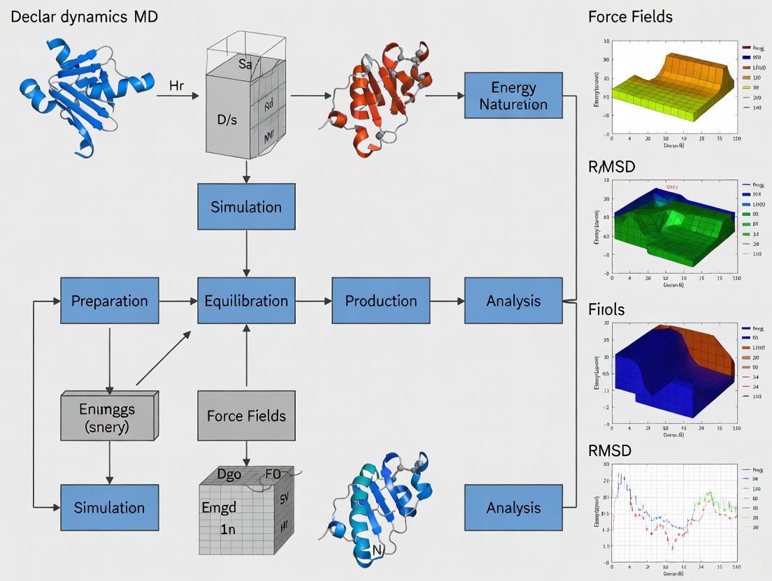
The following diagram illustrates the comprehensive workflow for a molecular dynamics simulation, highlighting the iterative process of force calculation and integration:

System Preparation and Equilibration Protocol

Initial System Setup:

• Obtain Initial Coordinates: Source atomic coordinates from experimental structures (Protein Data Bank), homology modeling, or previous simulations [8].
• Select Appropriate Force Field: Choose from established force fields (AMBER, CHARMM, GROMOS) based on the system composition and research objectives [8].
• Solvate the System: Embed the molecular system in an explicit solvent box (e.g., TIP3P, SPC/E water models) or use an implicit solvent model to reduce computational cost [10].
• Add Counterions: Introduce ions to neutralize system charge and mimic physiological ionic strength when relevant.

Energy Minimization:

• Perform steepest descent or conjugate gradient minimization to remove steric clashes and unfavorable contacts.
• Continue minimization until the maximum force falls below a specified tolerance (typically 100-1000 kJ/mol/nm).

System Equilibration:

• NVT Ensemble Equilibration: Run simulation with constant Number of particles, Volume, and Temperature (100-500 ps) using thermostats (Berendsen, Nosé-Hoover) to stabilize temperature at target value (e.g., 300K).
• NPT Ensemble Equilibration: Continue with constant Number of particles, Pressure, and Temperature (100-500 ps) using barostats (Parrinello-Rahman, Berendsen) to achieve correct density.

Production Simulation and Analysis

Production MD Simulation:

• Run simulation with appropriate timestep (typically 1-2 fs) using integration algorithms (Verlet, Leap-frog) [10].
• Apply constraint algorithms (SHAKE, LINCS) to allow longer timesteps by fixing fastest vibrations [10].
• Simulate for system-dependent duration (nanoseconds to microseconds) based on the biological process being studied [11].
• Save trajectory frames at regular intervals (1-100 ps) for subsequent analysis.

Trajectory Analysis Methods:

• Structural Stability: Calculate root-mean-square deviation (RMSD) of protein backbone atoms relative to starting structure.
• Flexibility Analysis: Compute root-mean-square fluctuation (RMSF) of residue positions to identify flexible regions.
• Conformational Sampling: Perform principal component analysis to identify essential dynamics and major conformational changes.
• Energetic Analysis: Calculate interaction energies between protein and ligands or specific residues.

Application to Small Protein Folding Research

MD simulations provide exceptional insights into protein folding mechanisms by offering atomic-level resolution of the folding process. The methodology enables researchers to characterize folding pathways, intermediate states, and transition states that are difficult to capture experimentally [11]. Several key studies demonstrate the power of MD in this domain:

Table 2: MD Simulations of Small Protein Folding Systems

Protein System	Simulation Details	Key Findings	Validation Approach
Villin Headpiece (HP-35)	20 × 1.0 μs simulations at 300K [11]	Refolding from extended states to structures with <1.0 Å Cα RMSD from crystal structure	Comparison to X-ray structure; identification of vital stability region consistent with mutagenesis [11]
Trp-cage	Multiple 20 ns simulations at 325K [11]	Successful refolding prediction with correct intramolecular contacts	Force field energy assessment; structural comparison to experimental data [11]
Chymotrypsin Inhibitor 2 (CI2)	200 ns simulation at 348K (Tm) [11]	Demonstration of microscopic reversibility - same contacts form during folding as break during unfolding	Comparison of physical properties, topology, and contact maps between starting and refolded states [11]
FBP28 WW Domain	Unfolding simulations under various denaturant conditions [11]	Transition state structure identification with first turn native-like while second turn forms during folding	Comparison to experimental Φ-values; validation of simulated TS structures [11]

The following diagram illustrates how MD simulations reveal the protein folding landscape through sampling of various conformational states:

Specialized Protocol for Protein Folding Simulations

Enhanced Sampling for Folding Studies:

• Temperature Replica Exchange MD: Run parallel simulations at different temperatures (300-500K) with periodic exchange attempts to enhance conformational sampling.
• Metadynamics: Apply biasing potential along carefully selected collective variables (e.g., radius of gyration, native contacts) to accelerate transitions over energy barriers.
• Umbrella Sampling: Use harmonic restraints along a reaction coordinate to calculate free energy landscapes for folding processes.

Folding Analysis Metrics:

• Q-value: Calculate fraction of native contacts formed relative to reference structure.
• Radius of Gyration: Monitor protein compactness throughout simulation trajectory.
• Secondary Structure Content: Track formation of α-helices and β-sheets using DSSP or similar algorithms.
• Contact Map Analysis: Identify specific residue-residue interactions characteristic of native state.

Successful implementation of MD simulations for protein folding research requires both specialized software and computational resources. The following table details essential components of the MD research toolkit:

Table 3: Essential Research Reagents and Computational Resources for MD Simulations

Resource Category	Specific Examples	Function/Purpose	Implementation Considerations
MD Software Packages	AMBER [8], CHARMM [8], NAMD [8], GROMACS	Primary simulation engines with optimized algorithms for different hardware architectures	AMBER/CHARMM offer specialized force fields; NAMD/GROMACS optimized for parallel computing
Force Fields	AMBER ff19SB, CHARMM36m, OPLS-AA/M	Parameter sets defining atomic interactions; some specifically optimized for proteins	CHARMM36m includes corrections for folded state stability; ff19SB improves backbone torsion accuracy
Solvent Models	TIP3P [10], SPC/E [10], TIP4P-EW, implicit solvent (GB/SA)	Water representation balancing accuracy and computational cost	Explicit models more accurate but computationally expensive; implicit models enable longer timescales
System Preparation Tools	CHARMM-GUI, PACKMOL, tleap	Generate initial simulation systems with proper solvation and ion placement	CHARMM-GUI provides web-based interface for complex system building
Analysis Software	MDAnalysis, VMD, CPPTRAJ, MDTraj	Trajectory analysis for structural, dynamic, and energetic properties	MDAnalysis offers Python API for customized analysis pipelines
Specialized Hardware	GPU Clusters [8], Anton Supercomputer [8]	Accelerate calculations through parallel processing	GPUs provide order-of-magnitude speedups [8]; Anton designed specifically for MD [8]
Validation Databases	Protein Data Bank, NMR chemical shifts, DEER distance distributions	Experimental data for force field validation and simulation assessment	Critical for ensuring simulated structures agree with experimental observations

Current Challenges and Methodological Limitations

Despite significant advances, several challenges remain in MD simulations of protein folding. The high computational demands typically restrict simulations to microsecond timescales, while many folding events occur on longer timescales [8] [11]. Current force fields, while continually improving, still employ approximations that neglect certain quantum mechanical effects, particularly regarding electronic polarization and hydrogen bonding [8] [10]. Additionally, adequate sampling of conformational space remains difficult, potentially leading to biased or incomplete understanding of folding landscapes [11].

Emerging approaches to address these limitations include the development of polarizable force fields [8], enhanced sampling algorithms [8], specialized hardware like Anton supercomputers [8], and machine learning approaches such as Microsoft's BioEmu biomolecular emulator that can rapidly sample protein conformational ensembles [7]. As these methodologies mature, MD simulations will continue to close the gap between computational modeling and experimental observations, providing increasingly accurate insights into the fundamental principles of protein folding with significant implications for drug discovery and structural biology [9] [11].

Molecular dynamics (MD) simulation serves as a "computational microscope," providing atomic-level insight into the process of protein folding, a fundamental event in biological activity [12] [13]. However, a significant challenge persists: the timescales of functionally important structural changes in proteins (microseconds to milliseconds) are often inaccessible to conventional MD simulations, which are typically limited to nanoseconds or microseconds due to computational constraints [12] [13]. This limitation arises from the phenomenon of "rare events," where the system becomes trapped in an energy basin, separated from other conformations by high energy barriers [12]. Consequently, conventional MD may fail to exhaustively sample the conformational space, leading to an inaccurate representation of the free-energy landscape (FEL), which is crucial for understanding folding mechanisms and stability [12]. This Application Note details enhanced sampling protocols and a novel AI-driven methodology designed to overcome these challenges, enabling accurate characterization of folding pathways and thermodynamics for small proteins.

Key Computational Challenges in Protein Folding

The Timescale and Sampling Problem

In MD simulations, the conformational space of a protein is characterized by numerous energy basins separated by energy barriers [12]. Crossing these high barriers is a rare event on the timescale of conventional MD, causing the simulation to become trapped in a non-representative subset of conformations [12]. This inefficient sampling makes it difficult to investigate thermodynamic properties like protein folding and binding affinity with conventional MD, as the simulation cannot adequately reflect equilibrium conditions [12].

The Energetic Accuracy Problem

The accuracy of an MD simulation is fundamentally tied to the force field—the model that calculates the forces governing atomic motions [13]. Classical force fields, while fast, are approximations and can lack chemical accuracy [4]. Although they have improved substantially, their imperfections introduce uncertainty into the simulation results [13]. In contrast, ab initio MD methods like density functional theory (DFT) provide high accuracy but are computationally prohibitive for large biomolecules, scaling with approximately O(N³) complexity for system size N [4].

Table 1: Comparison of MD Simulation Approaches for Protein Folding

Simulation Approach	Computational Cost	Energetic Accuracy	Key Limitation
Conventional (Classical) MD	Lower	Moderate (Approximate)	Inefficient sampling of rare events; force field inaccuracies [12] [13]
Ab Initio MD (e.g., DFT)	Exceedingly High (O(N³))	High (Chemically Accurate)	Not scalable to large proteins; a simulation of a 746-atom protein can take 92 minutes/step [4]
Enhanced Sampling MD	Moderate (Higher than conventional MD)	Dependent on underlying force field	Efficiency depends on the correct choice of reaction coordinate or collective variable [12]
AI-Driven Ab Initio MD (AI2BMD)	High, but significantly lower than DFT	High (Near Ab Initio Accuracy)	A 746-atom protein simulation takes ~0.125 seconds/step, >4 orders of magnitude faster than DFT [4]

Enhanced Sampling Protocols for Free-Energy Landscape Construction

Enhanced sampling methods are designed to facilitate barrier crossing, allowing the system to explore conformational space more efficiently and thus construct an accurate FEL [12]. The following protocols outline key methods.

Protocol: Umbrella Sampling for Free-Energy Reconstruction

Objective: To calculate the free-energy profile along a specific reaction coordinate (e.g., distance between protein domains, radius of gyration) [12].

• Define the Reaction Coordinate: Select a collective variable (ξ) that describes the progression from the unfolded to the folded state.
• Set Up Umbrella Windows: Perform multiple independent MD simulations, each with a harmonic bias potential applied to the reaction coordinate. The minima of these potentials should be spaced along the entire range of ξ, ensuring overlap between adjacent windows [12].
• Run Simulations: Conduct a conventional MD simulation for each window, recording the sampled values of ξ.
• Unbiased Analysis with WHAM: Use the Weighted Histogram Analysis Method (WHAM) to combine the data from all biased simulations, removing the effect of the umbrella potentials to reconstruct the unbiased probability distribution along ξ [12].
• Construct FEL: Calculate the free-energy landscape as F(ξ) = -kË…B T ln(P(ξ)), where P(ξ) is the unbiased probability distribution obtained from WHAM.

Protocol: Parallel Tempering (Temperature Replica Exchange)

Objective: To enhance conformational sampling by simulating replicas of the system at different temperatures, allowing exchanges between them [12].

• Define Temperature Ladder: Choose a set of temperatures ranging from the temperature of interest (e.g., 300 K) to a significantly higher temperature. The number of replicas and the temperature spacing should be chosen to ensure a non-negligible exchange rate [12].
• Run Concurrent Simulations: Simulate each replica independently at its assigned temperature.
• Attempt Replica Exchanges: Periodically attempt to swap the configurations of two adjacent replicas (i and j). The swap is accepted with a probability based on the Metropolis criterion, which ensures detailed balance is maintained [12].
• Analyze the Output: The trajectory at the temperature of interest (lowest temperature) will show enhanced sampling because it can access higher-temperature conformations during the exchange process. Analysis (e.g., FEL construction) is performed using snapshots from this replica.

Protocol: Essential Dynamics Sampling (EDS) for Protein Folding

Objective: To bias a simulation towards a target structure (e.g., the native fold) by utilizing collective motions derived from an equilibrated trajectory [14].

• Equilibrate and Perform ED Analysis: Run a conventional MD simulation of the native state. After equilibration, build and diagonalize the covariance matrix of the positional fluctuations of the Cα carbon atoms to obtain eigenvectors defining collective motions [14].
• Generate an Unfolded State (Expansion): Starting from the native structure, run an EDS simulation in "expansion mode," accepting only steps that increase the distance from the native structure in the subspace defined by the chosen eigenvectors [14].
• Perform Folding Simulation (Contraction): Using the unfolded structure from step 2, initiate an EDS simulation in "contraction mode." In this mode, a regular MD step is accepted only if it does not increase the distance from the native structure in the chosen subspace. If it does, the coordinates are projected onto a hypersphere maintaining the previous distance [14].
• Pathway Analysis: Analyze the resulting trajectory to identify folding intermediates and pathways, which can be compared with experimental data [14].

Diagram 1: Essential Dynamics Sampling Workflow for Protein Folding.

AI-AcceleratedAb InitioProtocol: AI2BMD

Objective: To simulate full-atom proteins with ab initio accuracy at a computational cost several orders of magnitude lower than DFT, enabling the observation of folding and unfolding [4].

• System Preparation:

  • Obtain the initial protein structure (folded, unfolded, or intermediate) from experimental data or prior simulations.
  • Solvate the protein in an explicit solvent model. AI2BMD uses the polarizable AMOEBA force field for water [4].

• AI-Driven Energy and Force Calculation:

  • The AI2BMD system fragments the protein into overlapping dipeptide units. This universal fragmentation approach covers only 21 types of protein units, making it generalizable [4].
  • At each simulation step, a machine learning force field (MLFF) potential, specifically ViSNet, calculates the energy and atomic forces. This MLFF is trained on a comprehensively sampled dataset of protein unit conformations calculated at the DFT level [4].
  • The MLFF encodes physics-informed molecular representations and computes four-body interactions with linear time complexity, providing highly accurate energy and force estimations [4].

• Simulation and Analysis:

  • Run the MD simulation using the AI2BMD potential. The system can explore the conformational space efficiently, reaching hundreds of nanoseconds and capturing folding/unfolding events [4].
  • Analyze the trajectory to derive accurate 3J couplings for comparison with NMR experiments, calculate free energies of folding, and estimate thermodynamic properties like melting temperature [4].

Table 2: Performance Metrics of AI2BMD vs. Density Functional Theory (DFT)

Protein (Number of Atoms)	AI2BMD Computation Time per Step (s)	DFT Computation Time per Step	Accuracy (Force MAE, kcal mol⁻¹ Å⁻¹)
Chignolin (175 atoms)	~0.072	21 minutes	1.974 (vs. 8.094 for MM) [4]
Albumin-Binding Domain (746 atoms)	~0.125	92 minutes	Not Specified [4]
Aminopeptidase N (13,728 atoms)	~2.610	>254 days (infeasible)	1.056 (vs. 8.392 for MM) [4]

Diagram 2: AI2BMD System Architecture for Ab Initio Accuracy.

The Scientist's Toolkit: Research Reagent Solutions

Table 3: Essential Computational Tools and Resources for Protein Folding MD

Research Reagent	Function in Protein Folding Simulation
GROMACS	A highly efficient software package for performing MD simulations, including energy minimization, equilibration, and production runs, with built-in analysis tools [15] [14].
MDAnalysis	A Python library for analyzing MD simulation trajectories, enabling the calculation of properties like RMSD, RMSF, and hydrogen bonds, and for performing dimensionality reduction [16].
AMOEBA Force Field	A polarizable force field used in the AI2BMD system to provide a more accurate treatment of electrostatic interactions in the explicit solvent environment [4].
ViSNet	A machine learning force field model that serves as the potential for AI2BMD. It uses physics-informed molecular representations to calculate energy and forces with ab initio accuracy [4].
Weighted Histogram Analysis Method (WHAM)	A statistical method critical for unbinding the data from umbrella sampling simulations to reconstruct the unbiased free-energy landscape [12].
VMD / PyMOL	Molecular visualization software used to visualize simulation trajectories, analyze conformational changes, interactively examine structures, and render high-quality images and animations [15].
Ethyl 4-(4-hydroxybutoxy)benzoate	Ethyl 4-(4-hydroxybutoxy)benzoate|CA
2-Methyl-5-nitropyrimidin-4(1H)-one	2-Methyl-5-nitropyrimidin-4(1H)-one, CAS:99893-01-3, MF:C5H5N3O3, MW:155.11 g/mol

In the realm of molecular dynamics (MD) simulations for small protein folding research, the accurate quantification of conformational sampling and convergence to native states is paramount. Key metrics including Root Mean Square Deviation (RMSD), Radius of Gyration (Rg), and Native Contact Formation provide indispensable, complementary insights into the structural, dynamic, and thermodynamic properties of folding proteins. These metrics serve as the primary validation tools for assessing both traditional MD and emerging machine learning (ML)-based simulation methods, enabling researchers to compare generated ensembles against reference experimental structures or long MD trajectories [17] [11]. Their collective application is crucial for advancing protocol development, force field refinement, and the understanding of folding mechanisms, with recent studies demonstrating their critical role in benchmarking novel coarse-grained models [18], latent diffusion generators [17], and accelerated sampling techniques [19].

Metric Definitions and Theoretical Foundations

Root Mean Square Deviation (RMSD)

RMSD quantifies the average displacement of atoms between a simulated protein structure and a reference structure (often the native state), providing a global measure of structural similarity. It is calculated using the formula:

\[RMSD = \sqrt{\frac{1}{N} \sum{i=1}^{N} \delta{i}^{2}}\]

where \(N\) is the number of atoms (typically Cα atoms for backbone comparison), and \(δ_i\) is the distance between atom \(i\) in the simulated and reference structures after optimal superposition. Lower RMSD values indicate closer convergence to the native fold. For example, successful refolding simulations of villin headpiece variants have reported Cα RMSD values below 1.0 Å relative to crystal structures [11]. RMSD is often tracked throughout a simulation trajectory to monitor folding progression and stability [19].

Radius of Gyration (Rg)

Radius of Gyration (Rg) describes the overall compactness of a protein structure, calculated as the root mean square distance of all atoms from their common center of mass:

\[Rg = \sqrt{\frac{\sum{i=1}^{N} mi |\mathbf{r}i - \mathbf{r}{\text{cm}}|^2}{\sum{i=1}^{N} m_i}}\]

where \(m_i\) is the mass of atom \(i\), \(r_i\) its position, and \(r_{\text{cm}}\) the center of mass. A decreasing Rg profile often signals hydrophobic collapse, an early stage in the folding pathway, while a stable, native-like Rg indicates proper tertiary packing. In folding studies of Protein L and CspTm, Rg measurements via single-molecule FRET revealed sequence-specific collapse at low denaturant concentrations, a finding corroborated by MD simulations [11].

Native Contact Formation

Native Contact Formation measures the fraction of non-local atomic contacts present in the native state that are formed during a simulation. A contact is typically defined when two heavy atoms (or Cβ atoms) are within a cutoff distance (e.g., 4.5 Å). The fraction of native contacts (Q) is calculated as:

\[Q = \frac{1}{N{\text{native}}} \sum{(i,j) \in \text{native}} \Theta( r{\text{cut}} - |r{i,j}| )\]

where \(N_{\text{native}}\) is the total number of contacts in the native structure, the sum runs over all native contact pairs (i,j), \(Θ\) is the Heaviside step function, \(r_{\text{cut}}\) is the cutoff distance, and \(r_{i,j}\) is the distance between atoms i and j in the simulated structure. This metric, often plotted as a time series or as part of a free energy landscape, is a sensitive indicator of folding cooperativity and the formation of specific stabilizing interactions. For instance, in AMD simulations of eight helical proteins, native contact analysis confirmed successful folding into stable native structures [19].

Table 1: Summary of Key Protein Folding Metrics and Their Interpretation

Metric	Structural Property Assessed	Typical Values (Folded)	Interpretation of Trends
RMSD (Cα atoms)	Global backbone conformation	< 2.0 – 3.0 Å [11]	Decreasing trend → Folding progression; Stable low value → Native state stability
Radius of Gyration (Rg)	Global compactness	Protein-specific, comparable to native structure Rg	Decreasing trend → Hydrophobic collapse; Stable value → Proper tertiary packing
Native Contact Fraction (Q)	Formation of specific tertiary interactions	~1.0 (fully folded)	Increasing trend → Cooperative folding; Stable high value → Native-like interaction network

Experimental Protocols and Workflows

Standard Protocol for Metric Calculation from MD Trajectories

The following workflow outlines the standard procedure for calculating key folding metrics from an MD simulation trajectory. Adherence to this protocol ensures consistency and reproducibility in analysis, which is critical for comparing results across different studies and simulation systems [17] [11].

• Trajectory Preparation: The raw MD trajectory must be pre-processed. This includes ensuring consistency in periodic boundary conditions, removing water and ions if the analysis is focused on the protein solute, and making sure the trajectory is correctly aligned to a reference frame to avoid artifacts from global rotation/translation.

• Structure Superimposition: For RMSD calculation, each frame of the trajectory is optimally superimposed onto the reference native structure. This step minimizes the RMSD by rotating and translating the simulated structure, thus isolating internal conformational changes from global motions. This is typically done using the Cα atoms of well-structured regions or the entire protein backbone.

• Metric Calculation:

  • RMSD: Compute the RMSD for the desired set of atoms (e.g., backbone, Cα, all heavy atoms) for every trajectory frame after superposition.
  • Rg: Calculate the radius of gyration for the protein (or a defined subdomain) for each frame.
  • Native Contacts: For each frame, compute the fraction of native contacts (Q) by comparing the current atomic distances to those in the native structure using a defined cutoff (e.g., 4.5 Ã… for Cβ atoms).

• Time-Series Analysis: Plot each metric as a function of simulation time. This visualizes the folding pathway, stability of the native state, and potential unfolding events.

• Statistical Analysis and Validation:

  • Convergence Analysis: Check if the metrics have reached a stable plateau, indicating convergence of the simulation in a particular state (folded, unfolded, or intermediate).
  • Ensemble Averaging: For multiple simulations (e.g., replica exchange or independent runs), average the metrics across the ensemble to get a more statistically robust estimate.
  • Cross-Validation with Experiment: Compare simulation-derived metrics with experimental data where available. For example, Rg from simulation can be compared to SAXS or FRET data [11], and native contact patterns can be indirectly validated against NMR data.

Application in Advanced ML-Based Generators

The validation of modern machine-learned ensemble generators relies heavily on these established metrics. For instance, the aSAM (atomistic structural autoencoder model) and AlphaFlow models are benchmarked by comparing the RMSD, RMSF (root mean square fluctuation), and native contact distributions of their generated ensembles against long, reference MD simulations [17]. Similarly, coarse-grained models like CGSchNet are evaluated on their ability to predict the correct folded state (low RMSD, high Q) and reproduce the fluctuations (related to Rg) and free energy landscapes of all-atom simulations [18].

Table 2: Representative Protocol Parameters from Recent Folding Studies

Study / Method	System	Simulation Time	Key Metric Validation
Accelerated MD (AMD) [19]	8 Helical Proteins (e.g., TC5B, 1WN8)	40-180 ns (folding event)	RMSD < 1.0 Ã…, native contact analysis, Rg convergence to native value
Machine-Learned CG (CGSchNet) [18]	Chignolin, TRP-cage, BBA, Villin	PT and long Langevin simulations	Free energy landscapes projected via RMSD and Q; comparison of folded state Rg
aSAM (Latent Diffusion) [17]	Test set from ATLAS/mdCATH	N/A (Ensemble generation)	Cα RMSD distribution (initRMSD), WASCO score for contacts, RMSF correlation
Brute-Force MD [11]	HP-36, CI2, FBP28 WW domain	200 ns - 1 μs	Cα RMSD, Rg, SASA, native secondary structure content

This table catalogs key computational tools, datasets, and software utilized in modern protein folding simulation research, as evidenced by recent literature.

Table 3: Key Research Reagents and Computational Solutions for Protein Folding Studies

Tool / Resource	Type	Primary Function in Folding Research	Example Use Case
GROMACS [20]	Software Package	High-performance MD simulation engine.	Performing all-atom, explicit solvent MD simulations for protein folding and unfolding [20] [21].
AMBER14SB [19]	Force Field	Defines potential energy terms for atoms in classical MD.	Providing parameters for protein and solvent interactions in folding studies of helical proteins [19].
ATLAS Database [17] [22]	MD Dataset	A large, curated set of all-atom MD simulations for diverse protein folds.	Training and benchmarking ML-based generative models like aSAM and AlphaFlow [17]; training predictors like PEGASUS [22].
mdCATH Dataset [17]	MD Dataset	MD simulations for thousands of globular domains at multiple temperatures.	Training temperature-conditioned generative models like aSAMt to study thermal behavior [17].
PEGASUS [22]	Deep Learning Tool	Predicts MD-derived flexibility metrics (RMSF, dihedral fluctuations) from sequence.	Rapidly estimating protein dynamics properties without running expensive simulations [22].
HADDOCK [20]	Docking Software	High Ambiguity Driven docking for biomolecular complexes.	Docking WRKY DNA-binding domains to W-box DNA prior to MD analysis [20].
CGSchNet [18]	Machine-Learned Force Field	A transferable coarse-grained force field for proteins.	Running efficient, predictive simulations of folding/unfolding for new protein sequences [18].

The integrated analysis of RMSD, Radius of Gyration, and Native Contact Formation remains the cornerstone of rigorous validation in protein folding simulations. As the field progresses with more complex systems, multi-scale models, and AI-driven generators [17] [18] [23], these metrics provide the essential, quantitative language for assessing the physical accuracy and predictive power of novel computational protocols. Their continued application, following standardized calculation workflows, is fundamental to bridging the gap between simulation and experiment, ultimately enhancing our understanding of protein folding mechanics and facilitating advances in molecular biology and drug development.

Practical MD Protocols: From System Setup to Production Runs

Within the broader context of investigating small protein folding mechanisms, the preparation of a biologically realistic system is a critical prerequisite for obtaining reliable molecular dynamics (MD) simulation data. The accuracy of folding pathways, free energy landscapes, and intermediate state identifications depends fundamentally on a properly constructed initial system. This protocol details the comprehensive procedure for converting a raw protein structure file (PDB) into a fully solvated, simulation-ready system using the GROMACS 2025 simulation package. The methodology is specifically optimized for small proteins, typically under 100 residues, where folding phenomena occur on tractable timescales. By following this structured approach, researchers can ensure their simulations of protein folding and unfolding events are conducted with atomic-level precision and thermodynamic rigor, providing a solid foundation for subsequent drug discovery and biomedical research applications.

The Scientist's Toolkit: Essential Research Reagents & Software

Table 1: Essential computational tools and files for GROMACS system preparation.

Component Name	Type	Primary Function in Protocol
GROMACS 2025	Software Suite	MD simulation engine used for all system preparation and simulation steps [24].
Protein Data Bank (PDB) File	Input File	Initial atomic coordinates of the protein structure (e.g., a small fast-folding protein like villin or WW domain).
Force Field (e.g., AMBER, CHARMM, OPLS)	Parameter Set	Defines the potential energy function, governing all interatomic interactions within the system [25] [26].
Solvent Model (e.g., SPC, TIP3P, TIP4P)	Parameter Set	Defines the water model used to solvate the protein, critical for simulating aqueous biological environments [25].
vdwradii.dat	Database File	Contains Van der Waals radii for atoms; used by gmx solvate to determine steric clashes during solvation [27].
Molecular Topology (.top)	Output/Input File	Describes all the molecules in the system and their interaction parameters, generated by gmx pdb2gmx [28].
GROMACS Structure (.gro)	Output/Input File	Standard coordinate file format in GROMACS containing atom positions, velocities, and box dimensions [28].
Run Input File (.tpr)	Output/Input File	A portable binary file containing all simulation parameters, generated by gmx grompp to serve as input for gmx mdrun [28].
Methyl 6-hydroxy-2-naphthimidate	Methyl 6-hydroxy-2-naphthimidate, CAS:765871-54-3, MF:C12H11NO2, MW:201.22 g/mol	Chemical Reagent
4-Amino-3-(tert-butyl)benzonitrile	4-Amino-3-(tert-butyl)benzonitrile|CAS 1369783-60-7	4-Amino-3-(tert-butyl)benzonitrile (CAS 1369783-60-7) is a sterically hindered aniline for advanced organic synthesis. For Research Use Only. Not for human or veterinary use.

The entire process of converting a PDB file into a solvated system suitable for MD simulation follows a sequential workflow. The following diagram maps the key stages, decision points, and primary outputs.

Detailed Step-by-Step Protocol

Step 1: Generate Protein Structure and Topology

The initial and crucial step involves processing the raw PDB file to generate a GROMACS-compatible structure file and a corresponding molecular topology. This is accomplished using the gmx pdb2gmx tool.

• Objective: To translate a PDB file of a protein into a GROMACS structure file (.gro) and a molecular topology file (.top). The topology contains a complete description of all interactions in the protein [28].
• Command:

• Key Interactive Selections:
  • Force Field (-ff): You will be prompted to select a force field (e.g., charmm27, amber99sb-ildn). The choice must be consistent with the intended scientific question and the force field's validation for protein folding studies [25] [26].
  • Water Model (-water): Select a water model (e.g., tip3p, spc/e). This model must be compatible with the chosen force field [25].
  • Terminal and Protonation States: The program will automatically assign charged termini (NH₃⁺ and COO⁻) for polypeptide chains. For histidine residues, it will select a protonation state (HIS, HIE, HID) based on optimal hydrogen-bonding geometry, which can be manually overridden with the -his flag [25].
• Critical Outputs:
  • conf.gro: The processed protein coordinates in GROMACS format.
  • topol.top: The system topology, which now includes the protein.
  • posre.itp: A file containing position restraints for the protein heavy atoms, useful for the initial equilibration stages.

Step 2: Define the Simulation Box

The protein must be placed in a finite simulation box for which periodic boundary conditions (PBC) are applied. The gmx editconf tool is used for this purpose.

• Objective: To center the protein in a simulation box of defined size and shape.
• Command:

• Parameter Rationale:
  • -c: Centers the protein in the box.
  • -d 1.2: Sets the distance between the protein and the box edge to 1.2 nm. This ensures a sufficient buffer of solvent around the protein, which is critical for accurate simulation of folding events by minimizing artificial periodicity effects.
  • -bt dodecahedron: Defines a dodecahedral box, which approximates a sphere and is more efficient for simulating globular proteins than a cubic box, as it requires fewer solvent molecules [28] [26].

Step 3: Solvate the System

The box containing the protein is now filled with solvent molecules using the gmx solvate tool. This step creates a realistic aqueous environment for the protein folding simulation.

• Objective: To add explicit solvent molecules to the simulation box, resulting in a solvated system.
• Command:

• Parameter Explanation:
  • -cp boxed.gro: Specifies the solute (the centered protein in its box) as the input coordinate file.
  • -cs spc216.gro: Specifies the solvent coordinate file. The default spc216.gro is a pre-equilibrated box of SPC water molecules, which can also be used for other 3-site models like TIP3P after a short equilibration [27].
  • -o solvated.gro and -p topol.top: Write the solvated coordinates and update the topology to include the added solvent molecules.
• Underlying Algorithm: The program removes any solvent molecule that overlaps with the solute, where overlap is defined as a distance between any solute and solvent atom less than the sum of their scaled Van der Waals radii. The radii are read from the vdwradii.dat database file and scaled by a default factor of -scale 0.57 to achieve a realistic density for proteins in water [27].

Table 2: Key options for the gmx solvate command.

Option	Default Value	Function	Consideration for Protein Folding
-cp	protein.gro	Input coordinate file of the solute (protein in a box).	Ensure the box is large enough to accommodate unfolding.
-cs	spc216.gro	Input coordinate file of the solvent.	Use a water model consistent with your force field selection in Step 1.
-scale	0.57	Scale factor for VdW radii from vdwradii.dat.	The default is optimized for a density of ~1000 g/L; altering this is generally not recommended [27].
-shell	0	Adds a water layer of specified thickness (nm) around the solute.	Useful for maintaining a spherical solvent shell during simulations.
-radius	0.105	Default VdW distance (nm) for atoms not found in vdwradii.dat.

This protocol provides a standardized, robust framework for preparing solvated systems of small proteins for molecular dynamics simulations focused on folding research. By meticulously executing these steps—generating a correct topology, defining an appropriate periodic box, and adding explicit solvent—researchers establish a physically accurate foundation for their simulations. The resulting system is primed for the subsequent stages of energy minimization and equilibration, which are necessary to relax any residual steric clashes and achieve stable temperature and density. A reliably prepared system is paramount for obtaining meaningful insights into protein folding dynamics, stability, and the atomic-level interactions that govern these fundamental biological processes.

In the realm of molecular dynamics (MD) simulations, the term "force field" refers to the combination of mathematical formulas and associated parameters that describe the potential energy of a biomolecular system as a function of its atomic coordinates [29]. The accuracy and reliability of any MD simulation, particularly for studying complex processes like protein folding, are fundamentally dependent on the choice of an appropriate force field. Force fields encode the physical chemistry of molecular interactions, balancing computational efficiency with physical accuracy to enable simulations of biological processes across relevant timescales. For researchers investigating small protein folding mechanisms, selecting a force field that accurately captures the delicate balance of interactions governing folding pathways, stable states, and transition barriers is paramount to generating biologically meaningful results.

The development of deep learning methods has revolutionized static protein structure prediction, but understanding dynamic folding processes still requires MD simulations that depend critically on force field accuracy [30] [18]. Modern protein folding studies demand force fields that can realistically simulate the transitions between multiple conformational states, including folded, unfolded, and intermediate structures, while maintaining computational feasibility [30]. This technical note provides a comprehensive comparison of three widely used biomolecular force fields—AMBER, CHARMM, and GROMOS—focusing on their application in small protein folding research, with practical implementation protocols for the GROMACS simulation package.

Force Field Comparison: AMBER, CHARMM, and GROMOS

Core Characteristics and Parameterization Philosophies

The AMBER, CHARMM, and GROMOS force fields represent distinct philosophical approaches to parameterization with different strengths and limitations for protein folding studies.

AMBER (Assisted Model Building with Energy Refinement) employs a functional form that includes bond stretching, angle bending, proper and improper dihedrals, and non-bonded interactions (electrostatics and Lennard-Jones) [29]. The parameterization of AMBER force fields combines quantum mechanical calculations with experimental data, making it particularly accurate for proteins and nucleic acids. Recent versions have significantly improved the treatment of backbone and side-chain torsions to better capture protein folding landscapes.

CHARMM (Chemistry at HARvard Macromolecular Mechanics) utilizes a similar functional form to AMBER but differs in its parameterization strategy, which places greater emphasis on reproducing experimental data for crystal structures, NMR data, and thermodynamic properties [29] [31]. This empirical approach aims to achieve balanced interactions between different molecular components, which is crucial for simulating complex processes like protein folding where multiple interaction types compete.

GROMOS (GROningen MOlecular Simulation) employs a different philosophy with a united-atom approach, representing aliphatic hydrogen atoms implicitly within their parent carbon atoms [29]. This reduces the number of particles in the system, offering computational advantages that enable longer timescale simulations. The parameterization of GROMOS force fields heavily relies on fitting to thermodynamic properties, particularly liquid thermodynamic data, which can enhance the accuracy of solvation effects in folding simulations.

Table 1: Fundamental Characteristics of Major Biomolecular Force Fields

Characteristic	AMBER	CHARMM	GROMOS
Atom Representation	All-atom	All-atom	United-atom (aliphatic hydrogens implicit)
Parameterization Basis	QM calculations + experimental data	Experimental data emphasis (crystal structures, NMR)	Liquid thermodynamic data
Functional Form	Comprehensive bonded and non-bonded terms	Comprehensive bonded and non-bonded terms	Simplified with united atoms
Computational Efficiency	Moderate	Moderate	Higher (fewer explicit particles)
Training & Validation	Combination of QM and experimental data	Heavy emphasis on experimental validation	Thermodynamic property fitting

Performance in Protein Folding Applications

The ability to accurately simulate protein folding remains a significant benchmark for force field validation. Recent studies have evaluated these force fields on their capacity to predict folded states, folding mechanisms, and the relative stability of different conformational states.

Small Protein Folding studies have revealed that all major force fields can generally fold small fast-folding proteins to their native states, but differences emerge in the precise characterization of folding pathways and the relative populations of intermediate states [18]. AMBER and CHARMM typically provide more detailed atomic resolution but at greater computational cost, while GROMOS offers advantages for sampling broader conformational spaces.

Disordered Proteins and Intrinsically Disordered Regions (IDRs) present particular challenges. The balance between protein-water and protein-protein interactions must be carefully parameterized to avoid artificial over-structuring or excessive disorder. Recent versions of AMBER (e.g., Amber99sb-ildn) and CHARMM (e.g., CHARMM36m) have incorporated adjustments to improve their performance for disordered systems [31].

Metastable State Prediction varies between force fields, with some demonstrating a tendency to stabilize specific types of non-native interactions. For example, certain AMBER parameters have shown improved capability in predicting metastable states of folded, unfolded, and intermediate structures, as well as fluctuations of intrinsically disordered proteins [18].

Table 2: Performance Characteristics for Protein Folding Studies

Performance Metric	AMBER	CHARMM	GROMOS
Native State Stability	Generally accurate with modern versions	Good with CHARMM36m	Variable depending on version
Folding Mechanism	Detailed but pathway-sensitive	Physically realistic	More approximate
Disordered Protein Handling	Good with -ildn variants	Excellent with CHARMM36m	Less accurate for IDPs
Secondary Structure Balance	Slight α-helix bias in older versions	Well-balanced in recent versions	Context-dependent
Computational Cost	Higher	Higher	Lower (united atom)
Timescale Access	Nanoseconds to microseconds	Nanoseconds to microseconds	Microseconds to milliseconds

Practical Implementation Protocols

System Setup and Simulation Workflow

Implementing successful protein folding simulations requires careful attention to system setup parameters and simulation protocols. The following workflow outlines a standardized approach applicable to small protein systems, with force field-specific considerations noted where appropriate.

Protein Structure Preparation begins with obtaining an initial protein structure, which can be derived from experimental data (e.g., PDB files) or predicted structures. For folding studies, starting from extended or unfolded states may be necessary to observe folding pathways. The PDB file provides atomic coordinates, residue names, and chain identifiers that form the foundation of your molecular system [31].

Force Field Selection requires consistent application throughout the simulation. As emphasized in the GROMACS documentation, "You should not mix and match force fields. Force fields are designed to be self-consistent, and will not typically work well with other force fields" [32]. This principle is critical for maintaining physical accuracy in your simulations.

Solvation and Ion Addition involves embedding the protein in an appropriate solvent environment, typically using water models specifically parameterized for each force field (e.g., TIP3P for AMBER and CHARMM, SPC for GROMOS). Ion concentration should be adjusted to physiological levels (typically 150mM NaCl) and the system neutralized to balance protein charges.

Simulation Parameters for Folding Studies

The molecular dynamics parameters (.mdp options) in GROMACS control the numerical integration and environmental conditions of your simulation [33]. The following table provides recommended settings for protein folding simulations.

Table 3: Key MDP Parameters for Protein Folding Simulations

Parameter Category	Setting	Rationale
Integrator	md-vv (velocity Verlet) or md (leap-frog)	Accurate integration with support for extended time steps
Time Step	2 fs (all-atom), 4 fs (united-atom with constraints)	Balance between numerical stability and computational efficiency
Temperature Coupling	Velocity rescaling (or Nose-Hoover)	Maintains constant temperature during folding
Pressure Coupling	Parrinello-Rahman (for production)	Maintains correct density without introducing artifacts
Constraint Algorithm	LINCS (all-atom), SETTLE (water)	Enables longer time steps by constraining bond vibrations
Non-bonded Interactions	PME for electrostatics, VdW cut-off 1.0-1.2 nm	Accurate treatment of long-range interactions
Neighbor Searching	Verlet list with 20-40 step update frequency	Computational efficiency with maintained accuracy

Enhanced Sampling for Folding Landscape Characterization

Standard MD simulations may struggle to sufficiently sample the complete folding landscape due to the high free energy barriers between states. Enhanced sampling techniques can improve conformational sampling:

Parallel Tempering/Replica Exchange MD involves running multiple replicas of the system at different temperatures, with periodic exchange attempts between neighboring temperatures. This approach allows conformations to overcome barriers at higher temperatures and populate low-energy states at lower temperatures, providing a more complete mapping of the folding landscape [18].

Metadynamics uses a history-dependent bias potential to discourage the system from revisiting previously sampled configurations, effectively "filling" free energy minima and driving transitions between states. This method is particularly useful for characterizing folding pathways and intermediate states.

Umbrella Sampling employs harmonic restraints along a predefined reaction coordinate (e.g., radius of gyration, native contacts) to enhance sampling in specific regions of conformational space. The potential of mean force (PMF) can then be reconstructed using the weighted histogram analysis method (WHAM) [32].

Successful implementation of protein folding simulations requires both computational tools and methodological knowledge. The following table outlines key resources for researchers.

Table 4: Essential Research Reagents and Computational Tools

Resource Category	Specific Tools	Function and Application
Simulation Software	GROMACS, AMBER, CHARMM/OpenMM, NAMD	MD simulation engines with varying performance characteristics
Force Field Databases	AMBER Parameter Database, CHARMM Parameter File, GROMOS Force Field Portal	Source of validated force field parameters
System Preparation	pdb2gmx (GROMACS), CHARMM-GUI, tleap (AMBER)	Tools for generating simulation topologies and initial coordinates
Analysis Tools	MDAnalysis, GROMACS analysis suite, VMD	Trajectory analysis, visualization, and property calculation
Enhanced Sampling	PLUMED, COLVARS	Libraries for implementing advanced sampling techniques
Specialized Databases	ATLAS, GPCRmd, MemProtMD [30]	MD trajectories and specialized parameters for specific protein classes
Validation Resources	PDBFlex, CoDNaS 2.0 [30]	Experimental data on protein flexibility and conformational diversity

Force Field Selection Guidelines

Choosing the appropriate force field requires balancing multiple considerations, including the specific research question, protein characteristics, and computational resources. The following decision framework provides guidance for selection:

For all-atom simulations with explicit solvent, AMBER and CHARMM offer the most detailed physical models, with CHARMM36m particularly effective for systems containing disordered regions and AMBER providing excellent performance for well-structured domains.

For enhanced sampling and longer timescales, the united-atom approach of GROMOS provides computational advantages that enable more extensive conformational sampling, though at the cost of atomic detail for aliphatic groups.

For membrane protein systems, specialized force fields and simulation protocols are required. As noted in membrane simulation guidelines, "Choose a force field for which you have parameters for the protein and lipids" and maintain consistency throughout the simulation [32].

Emerging Trends and Future Directions

The field of force field development continues to evolve, with several promising directions emerging:

Machine-Learned Force Fields represent a transformative approach, combining recent deep-learning methods with large and diverse training sets of all-atom protein simulations. These bottom-up coarse-grained force fields demonstrate chemical transferability and can be used for extrapolative molecular dynamics on new sequences not used during model parameterization [18]. These approaches show particular promise for predicting metastable states of folded, unfolded, and intermediate structures while being several orders of magnitude faster than all-atom models.

Integration with AI-Based Structure Prediction tools like AlphaFold creates opportunities for combining static structure prediction with dynamic ensemble characterization. While "AlphaFold only represents a single state of protein structure" and "cannot fully embody a native protein structure with conformational heterogeneity" [34], MD simulations with accurate force fields can expand these static pictures into dynamic ensembles.

Community-Wide Validation Efforts continue to refine force field performance through systematic assessment against experimental data. Researchers should remain informed about these validation studies and consider conducting their own validation against relevant experimental data for their specific protein systems.

In conclusion, the selection of AMBER, CHARMM, or GROMOS for small protein folding research depends on the specific research goals, protein characteristics, and computational resources. AMBER and CHARMM offer sophisticated all-atom representations with excellent accuracy for detailed mechanistic studies, while GROMOS provides computational advantages for enhanced conformational sampling. By following the protocols and decision framework outlined in this technical note, researchers can make informed choices that optimize the physical accuracy and computational efficiency of their protein folding simulations.

{# The document structure and formatting, including tables and dot code block, have been optimized for readability and adherence to user specifications. #}

{# Create a title page and introduction to frame the application note within the requested thesis context. #}

System Setup Essentials: Solvation, Ion Neutralization, and Energy Minimization

Application Notes and Protocols

Within the broader thesis on advancing molecular dynamics (MD) protocols for small protein folding research, the initial setup of the simulation system is a critical determinant of success. Accurate simulation of folding pathways, intermediate states, and free-energy landscapes fundamentally depends on a physically realistic and stable initial condition [35] [30]. This document provides detailed application notes and standardized protocols for the three foundational steps of system setup—solvation, ion neutralization, and energy minimization—with a specific focus on their pivotal role in studies of protein conformational dynamics and folding.

The Scientist's Toolkit: Essential Research Reagents and Materials

The following table details key software, force fields, and solvent models essential for setting up MD systems for protein folding research, as utilized in cited studies.

Table 1: Key Research Reagent Solutions for MD System Setup

Item Name	Function/Application	Example Use Case
GROMACS [35] [36] [37]	A high-performance molecular dynamics software package for simulating biomolecules.	Used for simulation box setup, solvation, ion addition, energy minimization, and production runs.
AMBER99SB Force Field [35] [37]	An all-atom force field for proteins, providing parameters for potential energy calculations.	Employed for topology generation of proteins to ensure accurate representation of intramolecular forces during folding simulations [37].
CHARMM36 Force Field [36] [38]	An all-atom force field for proteins, lipids, and nucleic acids.	Used for simulating membrane-associated proteins or complex biomolecular systems [38].
TIP3P Water Model [37]	A 3-site model for explicit solvent water molecules.	Used to solvate the protein system in a water box, creating a physiological environment for folding studies [37].
GAFF (General AMBER Force Field) [37] [38]	A force field for small organic molecules.	Applied to generate topologies for ligands or co-factors that may interact with the folding protein [37].
GB/SA Implicit Solvent [39]	A Generalized Born/Surface Area model for implicit solvation.	Used in constrained MD simulations to accelerate conformational sampling by approximating solvent effects without explicit water molecules [39].
martinize2 [40]	A script for automatically generating coarse-grained Martini model topologies from atomistic structures.	Used to set up systems for longer timescale simulations of large complexes when atomistic detail is not required [40].
9-(4-Fluorophenyl)-9H-carbazole	9-(4-Fluorophenyl)-9H-carbazole, CAS:57103-14-7, MF:C18H12FN, MW:261.3 g/mol	Chemical Reagent
(S)-2-Amino-4-cyanobutanoic acid	(S)-2-Amino-4-cyanobutanoic acid, CAS:6232-22-0, MF:C5H8N2O2, MW:128.13 g/mol	Chemical Reagent

Core System Setup Protocol

This section outlines a standardized workflow for preparing a solvated, neutralized, and minimized system, suitable for subsequent equilibration and production runs in protein folding simulations. The protocol is largely based on the high-throughput methodology detailed in the Galaxy HTMD tutorial [37] and incorporates parameters from recent literature [35].

The following diagram illustrates the logical sequence of the core system setup protocol, from initial structure preparation to a minimized system ready for equilibration.

Detailed Methodologies

3.2.1. Topology Generation The first step involves generating a topology file that defines the chemical structure and potential energy parameters for the protein and any ligands.

• Protein Topology: Use pdb2gmx (GROMACS) or an equivalent tool to generate the protein topology. A common command is: gmx pdb2gmx -f protein.pdb -o protein.gro -p topol.top -ff amber99sb -water tip3p [37]. This command processes the input PDB file, assigns force field parameters (e.g., AMBER99SB), and outputs the structure (.gro) and topology (.top) files.
• Ligand Topology: For non-standard residues or ligands, parameterize separately. Tools like acpype can be used with the GAFF force field to generate topologies compatible with AMBER-based force fields in GROMACS [37]. The protocol involves adding hydrogens at pH 7.0 and calculating partial charges (e.g., using the RESP method with bcc as a charge method) [37] [38].

3.2.2. Define Simulation Box The protein is centered in a periodic box with sufficient padding to prevent interactions with its periodic images.

• Procedure: Use the GROMACS editconf module: gmx editconf -f protein.gro -o protein_box.gro -bt cubic -d 1.0 -c [40]. The -d 1.0 flag places a 1.0 nm distance between the protein and the box edge. A cubic box is typical for globular proteins, while dodecahedral boxes can be more efficient for asymmetric molecules.

3.2.3. Solvation The box is filled with water molecules to create an aqueous environment.

• Procedure: Use the gmx solvate command: gmx solvate -cp protein_box.gro -cs spc216.gro -o solvated.gro -p topol.top [40]. This command fills the box (-cp) with water from a solvent coordinate file (-cs, e.g., water.gro for TIP3P) and updates the topology file with the number of added water molecules.

3.2.4. Ion Neutralization Ions are added to neutralize the system's net charge and achieve a physiological ion concentration.

• Procedure:
  • Generate a Binary Input File: gmx grompp -f ions.mdp -c solvated.gro -p topol.top -o ions.tpr -maxwarn 1 [40]. This step requires a parameter file (ions.mdp) with basic settings.
  • Add Ions: gmx genion -s ions.tpr -o neutralized.gro -p topol.top -pname NA -nname CL -neutral [40]. The -neutral flag instructs the tool to add enough ions to neutralize the system's net charge. For a specific concentration (e.g., 150 mM NaCl), the -conc flag can be added.

3.2.5. Energy Minimization Energy minimization relieves steric clashes and unfavorable geometric strain introduced during the setup process.

• Protocol Details: The minimization is typically performed using a steepest descent algorithm. A representative protocol, adapted from recent work on protein intermediate states, is summarized in the table below [35]. The goal is to reach a state where the maximum force is below a specified threshold, indicating a stable local energy minimum.

Table 2: Energy Minimization Protocol for Protein Folding Systems

Parameter	Specification	Rationale
Algorithm	Steepest Descent	Robust for initially highly distorted structures.
Maximum Steps	5000 steps or until convergence	Provides an upper limit; typically converges faster [35].
Energy Convergence	Maximum force < 1000 kJ·mol⁻¹·nm⁻¹	Standard initial tolerance for stable subsequent equilibration.
Force Tolerance	Maximum force < 5 kJ·mol⁻¹·nm⁻¹	A more rigorous convergence criterion used for atomistic protein folding simulations [35].

Experimental Protocols from Cited Literature

This section provides specific methodological details from recent research that successfully employed these setup essentials in protein folding and dynamics studies.

Discard-and-Restart MD for Intermediate States

A 2025 study by [35] developed an algorithm to sample protein intermediate states. Their system setup was critical for the subsequent short (10-20 ps) MD simulations.

• System Setup: Starting structures were energy-minimized using the steepest descent algorithm for 5000 steps or until the maximum force was lower than 5 kJ/mol/nm [35].
• Solvation: Simulations were performed in both implicit and explicit solvent, using the GROMACS simulation package [35].

Constrained MD Replica Exchange for Folding

A study on folding small proteins like Trp-cage used a constrained MD method (GNEIMO) with an implicit solvent [39].

• Solvation Model: The Generalized-Born Surface Area (GB/SA) implicit solvation model was used, with an exterior dielectric constant of 78.3 for water [39].
• Energy Minimization: The initial extended conformation was subjected to conjugate gradient minimization with a convergence factor of 10⁻² kcal/mol/Ã… in force gradient prior to simulation [39].

Molecular dynamics (MD) simulation is a powerful computational tool for studying protein folding, but its effectiveness is often limited by the timescales required to observe these complex processes. Conventional MD simulations can rarely overcome high energy barriers within practical computational timeframes, causing the system to become trapped in local energy minima. This article details two advanced sampling techniques—Replica Exchange Molecular Dynamics (REMD) and Constrained MD—that significantly enhance conformational sampling efficiency for small protein folding studies. These protocols are particularly valuable for drug development researchers investigating protein aggregation diseases or designing novel biomolecules.

Theoretical Foundation and Key Concepts

Replica Exchange Molecular Dynamics (REMD)

REMD is a hybrid method that combines MD simulation with Monte Carlo sampling to overcome energy barriers. In REMD, multiple non-interacting replicas of the same system are simulated simultaneously at different temperatures or with modified Hamiltonians. At regular intervals, exchanges between neighboring replicas are attempted with a probability derived from the Metropolis criterion:

[41]

For temperature REMD (T-REMD), this probability is calculated as:

[P(1 \leftrightarrow 2)=\min\left(1,\exp\left[ \left(\frac{1}{kB T1} - \frac{1}{kB T2}\right)(U1 - U2) \right] \right)]

where (T1) and (T2) are reference temperatures and (U1) and (U2) are instantaneous potential energies of replicas 1 and 2 respectively. After exchange, velocities are scaled by ((T1/T2)^{\pm0.5}) to maintain proper thermodynamics. [41]

For simulations with pressure coupling, the exchange probability extends to:

[P(1 \leftrightarrow 2)=\min\left(1,\exp\left[ \left(\frac{1}{kB T1} - \frac{1}{kB T2}\right)(U1 - U2) + \left(\frac{P1}{kB T1} - \frac{P2}{kB T2}\right)\left(V1-V2\right) \right] \right)]

where (P1) and (P2) are reference pressures and (V1) and (V2) are instantaneous volumes. [41]

Hamiltonian Replica Exchange (H-REMD)

Hamiltonian REMD modifies the force field parameters instead of temperature across replicas. The exchange probability becomes:

[41]

This approach is particularly efficient as it requires fewer replicas than T-REMD. A specialized variant focuses modifications on "hot spot" residues identified as crucial for structural stability through energy decomposition analysis. [42]

Constrained Molecular Dynamics

Constrained MD, also known as internal coordinate MD or torsion angle MD, reduces the number of degrees of freedom by imposing holonomic constraints on bond lengths and bond angles. The molecule is modeled as rigid bodies connected by flexible torsional hinges, decreasing computational cost by approximately an order of magnitude compared to all-atom Cartesian MD. This reduction allows for larger integration time steps (up to 5 fs) and enhances conformational sampling efficiency. [39]

REMD Protocol for Protein Folding Studies

System Preparation and Temperature Selection

The initial step involves constructing the system of interest. For peptide aggregation studies, this may involve placing monomers in a simulation box. Using a case study of hIAPP(11-25) dimer (sequence: RLANFLVHSSNNFGA) with terminal capping, the protocol begins with energy minimization of the initial structure. [43]

Optimal temperature distribution is critical for efficient replica exchange. The energy difference can be approximated as:

[41]

For a system with all bonds constrained, (N{df} \approx 2 N{atoms}). With (c = 2) for protein/water systems, the optimal temperature spacing gives (\epsilon \approx 1/\sqrt{N_{atoms}}). This spacing yields an exchange probability of approximately 0.135. Practical temperature ranges for small proteins typically span from 300K to 500K distributed across 8-16 replicas. [39]

Table 1: Temperature Distribution for REMD Simulations of Small Proteins

System Size (No. of Atoms)	Recommended Temperature Range (K)	Number of Replicas	Approximate Exchange Probability
Small peptide (< 1000)	300 - 450	6-8	0.15-0.25
Mini-protein (1000-3000)	300 - 500	8-12	0.12-0.20
Small protein (3000-5000)	300 - 550	12-16	0.10-0.18

Simulation Parameters and Exchange Protocol

REMD simulations are typically performed in the NPT ensemble using software such as GROMACS. Key parameters include:

• Integration time step: 2 fs with constraints applied to all bonds
• Thermostat: Langevin dynamics with collision frequency of 91 ps⁻¹
• Implicit solvent: GB/SA model with interior dielectric 1.75, exterior dielectric 78.3
• Non-bonded cutoff: 16-20 Ã… with smooth switching
• Exchange attempts: Every 1-2 ps of simulation time [44] [39]

The replica exchange pattern follows a neighbor-pair scheme where odd pairs (0-1, 2-3, ...) attempt exchange on odd attempts and even pairs (1-2, 3-4, ...) on even attempts. This approach ensures detailed balance while maintaining efficient temperature diffusion. [41]

Analysis Methods

Analysis of REMD trajectories includes:

• Free energy landscape calculation: Projection onto collective variables (e.g., RMSD, radius of gyration)
• Replica flow analysis: Monitoring temperature space diffusion to ensure proper mixing
• Cluster analysis: Identification of dominant conformational states using algorithms like k-means
• Principal Component Analysis (PCA): Projection of trajectories onto essential dynamics vectors [39] [43]

Constrained MD Protocol for Enhanced Sampling

System Setup and Hierarchical Clustering

Constrained MD simulations begin with an extended conformation of the peptide/protein, which undergoes energy minimization until convergence (e.g., force gradient < 10⁻² Kcal/mol/Å). The GNEIMO (Generalized Newton-Euler Inverse Mass Operator) method efficiently solves the coupled equations of motion in internal coordinates with O(N) computational cost. [39]

Hierarchical clustering schemes enhance sampling by "freezing and thawing" protein regions:

• All-torsion model: All torsional degrees of freedom are active
• Hierarchical clustering: Secondary structure motifs (e.g., helical regions) are treated as rigid clusters while sampling only connecting torsions
• Adaptive clustering: Clusters are updated based on emerging structural elements during simulation

Table 2: Constrained MD Parameters for Protein Folding Applications

Parameter	All-Torsion MD	Hierarchical Constrained MD
Degrees of Freedom	~10% of Cartesian MD	~5-7% of Cartesian MD
Integration Time Step	3-5 fs	3-5 fs
Solvation Model	GB/SA implicit solvent	GB/SA implicit solvent
Replica Exchange Temperatures	325K-500K (8 replicas)	325K-500K (8 replicas)
Exchange Attempt Frequency	Every 2 ps	Every 2 ps
Simulation Duration per Replica	10-20 ns	10-20 ns

Enhanced Sampling with Replica Exchange

Combining constrained MD with replica exchange (REMD-GNEIMO) further enhances sampling. The reduced degrees of freedom in constrained models decrease the number of required replicas approximately three-fold compared to all-atom REMD. A typical setup uses 8 replicas across 325K-500K with exchanges attempted every 2 ps. [39]

Research Reagent Solutions

Table 3: Essential Computational Tools for Advanced Sampling Simulations

Resource/Tool	Function	Application Example
GROMACS	MD simulation package with REMD implementation	Folding studies of hIAPP(11-25) fragment [43]
TINKER	MD package with constrained MD capabilities	Folding@home distributed computing projects [44]
GNEIMO method	O(N) computational cost constrained MD	Hierarchical folding of Trp-cage protein [39]
VMD	Molecular visualization and analysis	Trajectory visualization and system setup [43]
AMBER force fields	Protein force field parameters	Parm99 for folding simulations with GB/SA [39]
GB/SA implicit solvent	Implicit solvation model	OBC model for efficient folding simulations [39]

Case Studies and Applications

REMD for Peptide Aggregation

REMD successfully simulated the dimerization of hIAPP(11-25), a peptide relevant to type II diabetes. The protocol revealed the free energy landscape of early aggregation steps, identifying key intermediates in the formation of β-sheet-rich structures. This approach provides atomic-level insights into amyloid formation mechanisms that are challenging to capture experimentally. [43]

Constrained MD for Protein Folding

Constrained MD with replica exchange folded several small proteins starting from extended states:

• Polyalanine (20-mer): Achieved helical content formation with 6 replicas (300-450K)
• WALP16 transmembrane peptide: Folded in membrane-mimetic environment (dielectric constant 40)
• Trp-cage miniprotein: Sampled near-native structures with hierarchical clustering approaches [39]

Principal Component Analysis demonstrated that constrained MD explores wider conformational spaces than all-atom MD, with enhanced sampling of near-native structures. Cluster analysis of trajectories provided structural ensembles that align with zipping-and-assembly folding mechanisms. [39]

Hamiltonian REMD for Folding Hotspots

A specialized H-REMD protocol targeting folding "hot spots" enabled reversible folding/unfolding of Villin Headpiece HP35 and Protein A. The approach identified key residues through energy decomposition analysis, then applied soft-core potentials specifically to these residues across replicas. This targeted perturbation required fewer replicas while maintaining efficient sampling of folding transitions. [42]

REMD and Constrained MD provide complementary approaches for enhancing conformational sampling in protein folding studies. REMD excels at overcoming energy barriers through temperature cycling, while Constrained MD reduces computational cost through simplified molecular representations. Combining these methods with hierarchical clustering and Hamiltonian exchange schemes offers researchers a powerful toolkit for investigating protein folding landscapes, with significant applications in understanding protein misfolding diseases and designing therapeutic interventions.

The study of small, fast-folding proteins provides critical insights into the fundamental principles of protein folding, a key process in molecular biology with direct implications for understanding disease mechanisms and drug development. Proteins such as the Trp-cage, Villin headpiece, and WW domains have emerged as model systems in this field due to their small size, rapid folding kinetics, and well-characterized structures. These proteins serve as ideal benchmarks for developing and validating molecular dynamics (MD) simulation protocols, enabling researchers to bridge the gap between computational predictions and experimental observations. This application note details established experimental and computational protocols for investigating the folding mechanisms of these proteins, providing a structured framework for researchers in biophysics and drug development.

Protein Folding Case Studies

Trp-cage Mini-Protein

Background: The Trp-cage is a synthetically designed 20-residue mini-protein that folds on a microsecond timescale, making it an excellent subject for folding studies [45]. Its native structure comprises an N-terminal α-helix (residues 2-8), a 3₁₀-helix (residues 12-14), and a C-terminal polyproline motif (residues 17-19) that forms a hydrophobic cage around the sole tryptophan residue (Trp-6) [45].

Key Folding Insights:

• The folding mechanism involves complex kinetics that can be obscured when monitored by a single spectroscopic probe. Multi-probe approaches reveal that the 3₁₀-helix element unfolds independently at lower temperatures (below ~20°C) while the global cage structure remains stable, indicating localized conformational dynamics preceding global unfolding [45].
• The formation of the α-helix and the hydrophobic cage occurs simultaneously, as evidenced by identical relaxation rates measured via IR spectroscopy at 1580 cm⁻¹ (reporting on the Asp sidechain in the D9-R16 salt bridge) and 1612 cm⁻¹ (reporting on the ¹³C-labeled Ala residues in the α-helix) [45].
• φ-value analysis of the R16K mutant demonstrates that while this mutation decreases thermal stability (Tm reduction >9°C), the folding rate remains relatively unaffected, suggesting the transition state is not highly structured around this residue [45].

Table 1: Key Structural Elements and Their Roles in Trp-cage Folding

Structural Element	Residue Range	Role in Folding & Stability
α-helix	2-8	Early folding element; forms concurrently with hydrophobic cage
3₁₀-helix	11-14	Low stability element; unfolds independently at low temperatures
Polyproline region	17-19	Part of hydrophobic cage; provides structural scaffold
D9-R16 salt bridge	9 & 16	Key electrostatic interaction; stabilizes native fold
Hydrophobic core	3, 6, 12, 18, 19	Houses Trp-6; critical for stability

Villin Headpiece (HP35)

Background: The Villin headpiece is a 35-residue protein containing three α-helices. Its folding has been extensively studied through both experimental and computational approaches, with molecular dynamics simulations successfully capturing complete folding events [46] [47].

Key Folding Insights:

• Network analysis of reversible folding trajectories reveals a more complex folding landscape than suggested by traditional 2D projections. The native state (N) and primary intermediate state (I₁) show significant mingling and prevalent interstate transitions rather than clear separation [46].
• The folding landscape can be divided into four distinct regions: the folded native state (N), unfolded state (U), major intermediate region (I₁) characterized by a folded helix II/III segment, and a minor intermediate region (Iâ‚‚) [46].
• Deep enthalpic traps exist within the unfolded state ensemble, creating kinetic barriers that complicate the folding pathway. These structural features are often obscured in simplified landscape representations [46].
• Conventional MD simulations at 300K have achieved successful folding to native structures with Cα RMSD <0.5Ã… from the experimental structure, enabling atomic-level analysis of folding pathways [46].

Table 2: Villin Headpiece Folding States and Characteristics

State	Cα RMSD Segments A & B	Structural Features	Kinetic Role
Native (N)	RA < 2.0 Ã…, RB < 2.0 Ã…	All three helices formed	Stable folded basin
Intermediate I₁	RA > 2.0 Å, RB < 2.7 Å	Helix II/III segment folded	Primary intermediate
Intermediate Iâ‚‚	RA < 2.0 Ã…, RB > 2.0 Ã…	Other helical elements formed	Minor intermediate
Unfolded (U)	RA > 2.0 Ã…, RB > 2.7 Ã…	Lacking stable structure	Multiple enthalpic traps

WW Domain (Fip35)

Background: WW domains are approximately 35-residue modules that form three-stranded antiparallel β-sheets. These domains mediate protein-protein interactions and their folding exhibits notable heterogeneity [48].

Key Folding Insights:

• Folding proceeds along multiple distinct pathways with different formation orders of the two β-hairpins. Some trajectories show formation of the first hairpin early, while others form the second hairpin first [48].
• Structural heterogeneity is evident with the system folding into two distinct three-stranded β-sheet conformations: properly threaded native structures and "inverted" structures where key aromatic residues (Tyr-17, Phe-19) position differently relative to the β-sheet plane [48].
• At 300K with water viscosity, the mean first passage folding time is approximately 131 μs, comparable to experimental values of ~13 μs at 337K, validating the simulation approaches [48].
• Successful folding criteria include: Cα RMSD of β-sheet residues (6-11, 16-21, 25-28) <3.0Ã… and β-sheet conformation for residues 6-10, 17-20, and 26-27 confirmed by DSSP analysis [48].

Computational Protocols

Accelerated Molecular Dynamics (aMD) Protocol

Accelerated MD simulations enhance conformational sampling by adding a non-negative boost potential to the system when the potential energy falls below a reference energy, effectively reducing energy barriers between states [47].

Figure 1: aMD Simulation Workflow for Enhanced Sampling of Protein Folding

System Setup:

• Force Fields: AMBER ff14SBonlysc for general proteins; modified CHARMM22/AMBER ff99SBILDN for improved accuracy [47]
• Solvation: Implicit solvent (GB/SA) for sampling efficiency; explicit solvent for highest accuracy [47]
• Boost Parameters:
  • Dihedral boost: E_dihed = V_dihedavg + a₁ × N_res; α_dihed = aâ‚‚ × N_res/5
  • Dual boost (optional): E_total = V_totalavg + b₁ × N_atoms; α_total = bâ‚‚ × N_atoms
  • where N_res is residue count, N_atoms is total atoms [47]

Simulation & Analysis:

• Run aMD simulations for hundreds of nanoseconds to capture folding events
• Apply reweighting using cumulant expansion to the 2nd order to recover original free energy profiles [47]
• Identify native state within 0.2-2.1Ã… RMSD of experimental structures
• Analyze secondary structure formation and key residue interactions along folding pathways

AI-Driven Ab Initio Biomolecular Dynamics (AI2BMD)

AI2BMD represents a recent advancement that combines quantum chemistry accuracy with molecular dynamics scalability through machine learning force fields [4].

Protocol:

• Protein Fragmentation: Split proteins into overlapping dipeptide units (21 possible unit types covering all amino acid combinations) [4]
• Force Field Training: Train ViSNet models on comprehensively sampled protein unit dataset (20.88 million samples) with DFT-level accuracy [4]
• Energy/Force Calculation:
  • Potential energy MAE: 0.045 kcal mol⁻¹ (vs. 3.198 kcal mol⁻¹ for classical MM)
  • Force MAE: 0.078 kcal mol⁻¹ Å⁻¹ (vs. 8.125 kcal mol⁻¹ Å⁻¹ for classical MM) [4]
• Simulation Performance: Achieve ab initio accuracy with near-linear computational time scaling (e.g., 0.072s/step for Trp-cage vs. 21min/step for DFT) [4]

Monte Carlo Sampling Protocol

Monte Carlo methods provide an alternative to MD for extensive thermodynamic characterization without inherent timescale limitations [49].

Implementation:

• Force Field: AMBER99SB*-ILDN with generalized Born implicit solvent model [49]
• Sampling: 200 million MC steps covering temperature range 330K-410K [49]
• Analysis: Free energy landscape reconstruction, transition state identification, and per-residue stability profiling [49]

Experimental Protocols

Multi-Probe Temperature-Jump Spectroscopy

This experimental approach provides high structural resolution of folding kinetics by monitoring multiple spectroscopic signals simultaneously [45].

Sample Preparation:

• Utilize ¹³C=O labeled alanine variants (e.g., DAYAQWLKDGGPSSGRPPPS, A*=¹³C-Ala) to spectrally isolate α-helical segment signals [45]
• Prepare Trp-cage variants (TC5b, TC10b, Trp2-cage) at appropriate concentrations for spectroscopic measurements [45]

Data Collection:

• FTIR Spectroscopy: Collect amide I' band spectra (1600-1700 cm⁻¹) at varying temperatures [45]
• Specific Spectral Frequencies:
  • 1612 cm⁻¹: ¹³C-labeled Ala residues in α-helix
  • 1580 cm⁻¹: Asp sidechain (D9-R16 salt bridge)
  • 1664 cm⁻¹: 3₁₀-helix and disordered conformations [45]
• Temperature-Jump Kinetics: Monitor relaxation at each frequency after rapid heating (T-jump) [45]

Data Analysis:

• Fit kinetic traces to single or double exponential functions based on probing frequency
• Global analysis of rates across multiple probes to assign structural events
• Correlate temperature-dependent amplitude changes with structural stability

φ-Value Analysis

φ-value analysis probes the structure of the folding transition state by measuring the effects of point mutations on folding kinetics and stability [45].

Protocol:

• Design strategic point mutations (e.g., R16K in Trp-cage) that perturb specific interactions [45]
• Measure folding rates (k_f) and unfolding rates (k_u) for wild-type and mutant proteins
• Determine changes in folding free energy (ΔΔG) and activation energy (ΔΔG_‡)
• Calculate φ = ΔΔG_‡/ΔΔG, where φ ≈ 1 indicates native-like interaction in transition state, and φ ≈ 0 indicates absence of interaction [45]

The Scientist's Toolkit

Table 3: Essential Research Reagents and Computational Tools

Category	Item	Specification/Function	Application Examples
Protein Variants	¹³C-carbonyl labeled Ala peptides	Red-shifts amide I' band by ~40 cm⁻¹ for IR spectral isolation	Spectral separation of α-helix signals in Trp-cage [45]
	Strategic point mutants (e.g., R16K)	Perturbs specific interactions for φ-value analysis	Transition state structure mapping [45]
Computational Force Fields	AMBER99SB*-ILDN	Optimized for protein folding with implicit solvent	Monte Carlo sampling of folding landscapes [49]
	CHARMM22*	Modified backbone torsional potentials for transferability	Villin headpiece folding simulations [47]
	AMBER ff14SBonlysc	Balanced secondary structure propensity	Diverse set of fast-folding proteins [47]
Sampling Methods	Accelerated MD (aMD)	Dual-boost potential enhances barrier crossing	Microsecond folding in nanosecond simulations [47]
	AI2BMD	Machine learning force field with DFT accuracy	Ab initio folding with near-linear scaling [4]
	Monte Carlo	Dihedral moves with implicit solvent	Thermodependent free energy landscapes [49]
Analysis Tools	DSSP	Secondary structure assignment	β-sheet formation criteria in WW domains [48]
	VISONE/NetworkX	Network analysis and visualization	Folding pathway identification from MD trajectories [46]
	Cα RMSD clustering	Structural similarity measurement (2.0Å cutoff)	Conformational state classification [46]
6-(Bromomethyl)-2,2'-bipyridine	6-(Bromomethyl)-2,2'-bipyridine, CAS:83478-63-1, MF:C11H9BrN2, MW:249.11 g/mol	Chemical Reagent	Bench Chemicals
4-(bromomethyl)-N,N-dimethylaniline	4-(Bromomethyl)-N,N-dimethylaniline|CAS 102236-12-4		Bench Chemicals

The integrated application of advanced computational methods and sophisticated experimental techniques has significantly advanced our understanding of small protein folding mechanisms. Trp-cage, Villin headpiece, and WW domains continue to serve as critical model systems for developing and validating new approaches in this field. The protocols outlined herein provide researchers with comprehensive methodologies for investigating protein folding dynamics, from atomic-level simulation to experimental validation. As computational power increases and algorithms refine, these integrated approaches will enable increasingly accurate predictions of protein folding behavior, with important implications for protein design and therapeutic development.

Overcoming Limitations: Strategies for Enhanced Sampling and Accuracy

Molecular dynamics (MD) simulation is a powerful computational technique for studying protein folding, providing atomic-resolution insights into folding pathways and mechanisms. However, a significant challenge persists: the timescales accessible to conventional MD (cMD) simulations are often orders of magnitude shorter than the biological folding times of even small, fast-folding proteins [50]. This timescale gap hinders our ability to obtain sufficient sampling for statistically meaningful conclusions. Specialized hardware, particularly Graphics Processing Units (GPUs), and novel machine learning algorithms are now bridging this gap, enabling microsecond to millisecond simulation timescales to become routine. This Application Note details protocols for leveraging these technologies to accelerate protein folding research, providing benchmarks and implementation guidelines for researchers.

Hardware Landscape for Accelerated MD

GPU Selection for Molecular Dynamics

Selecting the appropriate GPU is critical for maximizing simulation throughput. The choice involves a trade-off between computational power, memory capacity, and precision capabilities. The table below summarizes recommended GPUs for MD simulations based on key performance metrics.

Table 1: GPU Recommendations for Molecular Dynamics Simulations

GPU Model	Architecture	Key Feature	VRAM	Target Use-Case
NVIDIA RTX 4090	Ada Lovelace	16,384 CUDA cores	24 GB GDDR6X	Cost-effective performance for most systems [51]
NVIDIA RTX 6000 Ada	Ada Lovelace	18,176 CUDA cores	48 GB GDDR6	Large-scale, memory-intensive simulations [51]
NVIDIA A100/H100	Ampere/Hopper	High FP64 throughput	40-80 GB HBM2e	FP64-dominated codes (e.g., DFT/ab-initio) [52]
NVIDIA L40S	Ada Lovelace	Balanced data-center GPU	48 GB GDDR6	Batch homology searches & cloud deployment [53]

Precision Considerations in Hardware Selection

A crucial first question when selecting hardware is whether the simulation code requires true double precision (FP64). Many MD codes like GROMACS, AMBER, and NAMD have mature, mixed-precision GPU acceleration pathways that deliver excellent performance and accuracy on consumer and workstation GPUs (e.g., RTX 4090/5090) [52]. These GPUs offer high single-precision (FP32) performance, which is leveraged efficiently.

However, codes that mandate FP64 throughout the calculation, such as CP2K, Quantum ESPRESSO, and VASP, will experience significant bottlenecks on consumer GPUs, which have intentionally limited FP64 throughput. For these applications, data-center GPUs like the NVIDIA A100 or H100 or traditional CPU clusters are more appropriate [52].

Table 2: Precision Requirements for Common Scientific Software

Software/Method	Expected Precision	Hardware Fit	Notes
GROMACS, AMBER, NAMD	Mixed (FP32/FP64)	Excellent on consumer/workstation GPUs	Mature GPU-offloading for non-bonded forces, PME, updates [52]
DeepJump, BioEmu	FP32 (typical for DL)	Excellent on consumer/workstation GPUs	High computational intensity suited for high FP32 throughput [54] [7]
CP2K, Quantum ESPRESSO	Double (FP64)	Poor on consumer GPUs; Good on A100/H100	Requires high FP64 throughput, otherwise speedups are limited [52]

Accelerated Sampling Methodologies & Protocols

AI-Driven Dynamics Emulation

A paradigm shift is underway from physics-based integration to data-driven emulation. Models like DeepJump use Euclidean-Equivariant Flow Matching to learn protein conformational dynamics from existing trajectory data. Once trained, they can predict long-timescale dynamics from short, initial simulations, achieving computational accelerations of up to ≈1000x compared to traditional MD while effectively recovering long-timescale kinetics [54].

Protocol 1: Running Dynamics with DeepJump-style Models

• Input Preparation: Provide a starting conformational state, protein sequence, and a desired "jump time" (δ).
• Model Conditioning: A conditioning encoder processes the current state, sequence, and jump time into a latent representation.
• Conformation Generation: A transport network iteratively updates a noised version of the input state to generate the predicted conformation at the future time step. This architecture is inherently Euclidean-equivariant, ensuring physical correctness of the generated structures [54].
• Trajectory Construction: Iteratively apply the model using the predicted state as the new input to generate a long-timescale trajectory.

Application Note: These models are particularly powerful for ab initio folding simulations, enabling the prediction of folding pathways and native states from extended conformations [54].

Enhanced Sampling with Accelerated MD

Accelerated MD (aMD) is an established enhanced sampling technique that works by adding a non-negative boost potential to the system's original potential energy when it falls below a reference energy. This effectively lowers energy barriers, increasing the rate of transitions between low-energy states without requiring pre-defined reaction coordinates [47].

Protocol 2: Setting up a Dual-Boost aMD Simulation

This protocol uses the AMBER software package as a reference.

• System Preparation: Prepare the protein solvated in an explicit solvent box, followed by standard energy minimization and equilibration under NVT and NPT conditions.
• Boost Potential Calculation: The dual-boost method applies two boost potentials:
  • Dihedral Boost: Applied to all dihedral angles in the system. Parameters are calculated as:
    • Edihed = Vdihed_avg + a1 * Nres
    • αdihed = a2 * Nres / 5
  • Total Boost: Applied to the total potential energy of the system. Parameters are calculated as:
    • Etotal = Vtotal_avg + b1 * Natoms
    • αtotal = b2 * Natoms Here, Nres is the number of residues, Natoms is the total number of atoms, and Vdihed_avg and Vtotal_avg are average energies from a short cMD run. The coefficients a1, a2, b1, b2 are user-defined and control the acceleration level [47].
• Production Simulation: Run the aMD production simulation using the calculated boost parameters. A 2 fs timestep is typical, with the SHAKE algorithm applied to bonds involving hydrogen.
• Reweighting (for Free Energy): To recover the original canonical distribution, reweighting is essential. The Cumulant Expansion to the 2nd order method has been shown to greatly improve the accuracy of free energy calculations from aMD simulations [47].

Machine-Learned Coarse-Grained Models

Machine-learned coarse-grained (CG) models offer another path to acceleration by reducing the number of degrees of freedom. A key advancement is the development of transferable CG force fields, such as CGSchNet, which are trained on all-atom simulation data from diverse proteins [18].

Protocol 3: Simulating with a Transferable Coarse-Grained Model

• Model Selection & Setup: Choose a pre-trained, transferable model. The model in [18] uses a bottom-up force-matching approach on a Cα representation.
• Input Definition: Provide the amino acid sequence of the protein to be simulated. No initial structure is strictly required for folding studies.
• Simulation Execution: Run molecular dynamics using the learned CG force field. These simulations can be several orders of magnitude faster than all-atom MD.
• Analysis: The model can predict metastable folded, unfolded, and intermediate states, fluctuations of intrinsically disordered regions, and relative folding free energies of mutants, demonstrating performance comparable to all-atom MD for many applications [18].

Integrated Workflow for Protein Folding Analysis

The following diagram illustrates a modern, integrated workflow that leverages GPU acceleration and specialized algorithms at multiple stages, from sequence input to dynamic analysis.

Table 3: Key Software and Data Resources for Accelerated Protein Folding Studies

Resource Name	Type	Function & Application	Acceleration Feature
DeepJump [54]	AI Dynamics Model	Predicts long-timescale protein conformational dynamics from short trajectories.	Flow Matching; ≈1000x reported speedup.
BioEmu [7]	Biomolecular Emulator	Samples equilibrium distribution of protein conformations from sequence via diffusion.	Single GPU; generates 10,000 structures in minutes/hours.
CGSchNet [18]	Coarse-Grained Force Field	Transferable CG model for MD; predicts folded states, IDP fluctuations, and ΔΔG.	Orders of magnitude faster than all-atom MD.
MMseqs2-GPU [53]	Homology Search Tool	Rapid generation of Multiple Sequence Alignments (MSAs) for structure prediction inputs.	6x faster single-protein search vs. 2x64-core CPU [53].
AMBER, GROMACS, NAMD [51] [52]	Molecular Dynamics Software	Standard MD simulation packages with mature GPU acceleration.	Offloads force calculation, PME, updates to GPU.
ATLAS Database [30]	MD Trajectory Database	Repository of diverse protein simulations for training AI models or validation.	Provides pre-computed data, saving simulation time.
GPCRmd [30]	Specialized MD Database	Simulation trajectories for G-protein coupled receptors.	Focused resource for membrane protein studies.

Enhanced Sampling Methods for Rare Events and Free Energy Calculations

Molecular dynamics (MD) simulation has emerged as a crucial computational microscope for studying biological processes at atomic resolution. However, the utility of conventional MD is often limited by the timescale gap between simulated and biologically relevant processes. Rare events, such as protein folding and ligand unbinding, occur on timescales from microseconds to seconds, but all-atom MD simulations are typically limited to nanosecond or microsecond scales due to computational constraints [55]. This limitation arises from the rough energy landscapes of biomolecules, characterized by many local minima separated by high energy barriers that trap conventional simulations [55]. Enhanced sampling methods have been developed to address this fundamental challenge, enabling efficient exploration of configuration space and accurate free energy calculations for small protein folding systems.

Theoretical Foundations of Enhanced Sampling

The Sampling Problem in Biomolecular Simulations

Biomolecular systems exhibit complex, multidimensional free energy landscapes with numerous metastable states. The probability of crossing energy barriers higher than 5-10 kBT decreases exponentially with barrier height, making spontaneous barrier crossing statistically improbable in short simulations [56]. For example, protein folding barriers of 8-12 kcal/mol correspond to timescales of milliseconds or longer, creating a significant sampling challenge [56]. This timescale gap necessitates enhanced sampling techniques that accelerate barrier crossing while maintaining correct thermodynamics and kinetics where possible.

Classification of Enhanced Sampling Methods

Enhanced sampling methods can be broadly categorized into two classes: collective variable (CV)-based methods and unconstrained methods. CV-based methods like metadynamics and umbrella sampling require predefined reaction coordinates and bias the simulation along these coordinates to enhance barrier crossing [56]. Unconstrained methods like replica exchange molecular dynamics (REMD) do not require prior knowledge of reaction coordinates and instead enhance sampling through modified Hamiltonians or temperatures [56].

Table: Classification of Enhanced Sampling Methods

Method Type	Representative Methods	Key Characteristics	Primary Applications
CV-based methods	Metadynamics, Umbrella Sampling, Adaptive Biasing Force	Require predefined collective variables; "fill" free energy wells	Protein-ligand binding, conformational transitions
Unconstrained methods	REMD, Accelerated MD, Self-guided MD	No predefined CVs needed; modify temperature or potential energy	Protein folding, unexplored transitions
Structure-based models	WSME-L, AI2BMD	Incorporate native structure information; statistical mechanical	Folding mechanisms, free energy landscapes

Key Enhanced Sampling Methods

Replica Exchange Molecular Dynamics (REMD)

REMD, also known as parallel tempering, employs multiple replicas of the system simulated in parallel at different temperatures [55] [56]. Exchanges between replicas at neighboring temperatures are attempted periodically with acceptance probability:

[ w(X \rightarrow X') = min(1, \exp[(\betam - \betan)(V(r[i]) - V(r[j]))]) ]

where (\betam = 1/kBT_m) and (V(r[i])) is the potential energy of replica i [56]. This enables configurations to perform a random walk in temperature space, preventing trapping in local minima. The temperature range must be carefully selected, as setting the maximum temperature too high can reduce efficiency compared to conventional MD [55]. REMD has been successfully applied to study folding mechanisms of peptides and small proteins, with variants including Hamiltonian REMD (H-REMD) for enhanced conformational sampling [55].

Metadynamics

Metadynamics enhances sampling by adding a history-dependent bias potential along predefined collective variables (CVs) that discourages revisiting of previously sampled configurations [55]. The method effectively "fills" free energy wells with "computational sand," forcing the system to explore new regions of configuration space [55]. The bias potential is typically constructed as a sum of Gaussian functions deposited along the trajectory in CV space:

[ V{bias}(s,t) = \sum{t'=τ,2τ,...} w \exp\left(-\frac{|s-s(t')|^2}{2σ^2}\right) ]

where (s) represents the collective variables, (w) is the Gaussian height, and (σ) determines their width. After sufficient simulation time, the bias potential converges to the negative of the underlying free energy surface, enabling free energy estimation. Metadynamics has proven particularly effective for studying protein-ligand binding, conformational changes, and protein folding [55].

Simulated Annealing

Simulated annealing mimics the physical annealing process in metallurgy by introducing an artificial temperature that gradually decreases during the simulation [55]. This approach allows the system to overcome energy barriers at high temperatures and settle into low-energy configurations as the temperature decreases. Variants include classical simulated annealing (CSA), fast simulated annealing (FSA), and generalized simulated annealing (GSA), with GSA being particularly suitable for large macromolecular complexes at relatively low computational cost [55].

Machine Learning-Enhanced Approaches

Recent advances integrate machine learning with enhanced sampling. AI2BMD combines protein fragmentation with machine learning force fields to achieve ab initio accuracy while reducing computational time by several orders of magnitude compared to density functional theory [4]. The system fragments proteins into dipeptide units, calculates intra- and inter-unit interactions using a ViSNet model, and assembles them to determine total protein energy and forces [4]. CGSchNet uses graph neural networks to learn effective interactions for coarse-grained simulations, enabling accurate modeling of protein folding and dynamics while operating significantly faster than all-atom MD [6].

Application Notes for Small Protein Folding

Selecting Appropriate Enhanced Sampling Methods

Method selection should be guided by the specific characteristics of the protein system and research question. For small single-domain proteins with unknown reaction coordinates, REMD is often preferred as it doesn't require predefined CVs [55] [56]. For studying specific transitions like folding/unfolding or ligand binding where relevant CVs are known, metadynamics provides targeted enhanced sampling [55]. When high accuracy is critical and sufficient training data exists, AI2BMD offers ab initio quality for systems up to 10,000 atoms [4].

Table: Method Selection Guide for Small Protein Folding

Protein Characteristics	Recommended Method	Simulation Protocol	Expected Performance
Small single-domain, <100 residues	REMD	24-64 replicas; temperature range 300-500K; exchange attempts every 1-2ps	Excellent for folding mechanism identification
System with known reaction coordinates	Metadynamics	Well-tempered metadynamics; Gaussian deposition every 1ps; height 0.1-0.5 kJ/mol	Accurate free energy barriers
Large systems >1000 atoms where atomic accuracy critical	AI2BMD	Protein fragmentation; ML force field; explicit solvent with AMOEBA	Near-DFT accuracy with 10^6× speedup
Rapid screening of multiple mutants	WSME-L model	Structure-based statistical mechanical model; exact analytical solution	Folding pathways and intermediates

Practical Implementation Considerations

Successful enhanced sampling requires careful parameter selection. For REMD, temperature spacing should ensure exchange probabilities of 20-40%, typically achieved with 5-10K intervals for small proteins [55]. For metadynamics, Gaussian width should be 10-20% of CV fluctuation in the unbiased system, with height adjusted to provide sufficient bias without overwhelming natural dynamics [55]. Simulation length must ensure convergence, typically 100-500ns per replica for small protein folding, with convergence assessed through multiple independent runs and statistical analysis.

Experimental Protocols

REMD Protocol for Small Protein Folding

Step 1: System Preparation

• Obtain initial protein structure from PDB or predicted structure
• Solvate in appropriate water box (minimum 10Ã… padding)
• Add ions to neutralize system and achieve physiological concentration (150mM NaCl)
• Energy minimization using steepest descent (maximum force <1000 kJ/mol/nm)

Step 2: Equilibration

• NVT equilibration for 100ps with protein heavy atoms restrained (force constant 1000 kJ/mol/nm²)
• NPT equilibration for 100ps with protein heavy atoms restrained (force constant 1000 kJ/mol/nm²)
• NPT production without restraints for 1-5ns at target temperature

Step 3: REMD Setup

• Determine temperature distribution using temperature predictor tools or preliminary simulations
• Typically 24-64 replicas for small proteins (50-100 residues)
• Temperature range: 300-500K with exponential distribution
• Set exchange attempt frequency: every 1-2ps
• Simulate each replica for 100-500ns depending on system complexity

Step 4: Analysis

• Calculate free energy surfaces using weighted histogram analysis method (WHAM)
• Identify folding intermediates and transition states
• Compute folding rates from free energy barriers using Kramers' theory

Metadynamics Protocol for Folding/Unfolding

Step 1: Collective Variable Selection

• Identify appropriate CVs (e.g., native contacts, radius of gyration, secondary structure content)
• Validate CVs through preliminary short simulations
• For small proteins, 2-3 CVs typically sufficient to describe folding process

Step 2: Well-Tempered Metadynamics Parameters

• Gaussian height: 0.1-0.5 kJ/mol
• Gaussian width: 10-20% of CV fluctuations in unbiased simulation
• Deposition rate: Every 1-2ps
• Bias factor: 10-30 for enhanced sampling without loss of accuracy

Step 3: Simulation and Monitoring

• Run simulation until free energy estimate converges (typically 200-500ns)
• Monitor CV distributions and bias potential growth
• Perform multiple independent runs to assess reproducibility

Step 4: Free Energy Analysis

• Reconstruct free energy surface from bias potential
• Identify metastable states, minima, and barriers
• Calculate folding thermodynamics (ΔG, stability)

The Scientist's Toolkit

Table: Essential Research Reagent Solutions for Enhanced Sampling Studies

Tool/Resource	Type	Function	Application Context
GROMACS	Software	MD simulation package with enhanced sampling implementations	REMD, metadynamics for protein folding
PLUMED	Plugin	Collective variable analysis and enhanced sampling	CV-based methods (metadynamics, umbrella sampling)
AI2BMD	ML Force Field	Ab initio accuracy biomolecular MD	High-accuracy protein folding simulations
WSME-L Model	Statistical Model	Structure-based folding prediction	Rapid prediction of folding mechanisms
Chignolin	Model System	Fast-folding mini-protein	Method validation and benchmarking
AMBER/CHARMM	Force Fields	Empirical molecular energy functions	Classical MD simulations with enhanced sampling
Phenol, 4-[(4-ethoxyphenyl)azo]-	Phenol, 4-[(4-ethoxyphenyl)azo]-, CAS:2496-26-6, MF:C14H14N2O2, MW:242.27 g/mol	Chemical Reagent	Bench Chemicals
2-isopropyl-4-phenyl-1H-imidazole	2-isopropyl-4-phenyl-1H-imidazole, CAS:31787-73-2, MF:C12H14N2, MW:186.25 g/mol	Chemical Reagent	Bench Chemicals

Visualization of Enhanced Sampling Workflow

Enhanced sampling methods have transformed our ability to study protein folding processes that were previously inaccessible to computational modeling. The choice of method depends on system size, available structural knowledge, and computational resources. REMD remains highly effective for small proteins without predefined reaction coordinates, while metadynamics offers targeted sampling for specific transitions. Emerging machine learning approaches like AI2BMD and CGSchNet promise to further bridge the accuracy-efficiency gap, enabling ab initio quality simulations of large systems. As these methods continue to evolve, they will provide increasingly powerful tools for understanding protein folding mechanisms and designing novel therapeutics.

Addressing Force Field Imperfections and Solvent Model Choices

Molecular dynamics (MD) simulation is an indispensable tool for studying small protein folding, yet the accuracy of these simulations is fundamentally governed by the choice of force field and solvent model. Traditional force fields exhibit systematic deficiencies, particularly when modeling complex phenomena like intrinsically disordered proteins (IDPs) or charge-transfer reactions. This application note details these imperfections, documents advanced solutions—including machine-learned force fields and improved solvent models—and provides validated protocols to guide researchers in selecting and applying these tools for robust protein folding research.

Table 1: Summary of Advanced Force Fields and Their Applications

Force Field / Model	Type	Key Strengths	Reported Limitations / Considerations	Primary Application in Protein Research
Neural Network Force Fields (e.g., NeuralIL) [57]	Machine-Learned Atomistic	DFT-level accuracy; captures polarization, proton transfer, and weak hydrogen bonds.	10-100x slower than classical FFs; requires specialized training data.	Charged fluids, ionic liquids, and systems with chemical reactivity.
Machine-Learned Coarse-Grained (e.g., CGSchNet) [18]	Machine-Learned Coarse-Grained	Transferable across sequences; orders of magnitude faster than all-atom MD.	Loss of atomic detail; performance may vary with complex structural motifs.	Folding/metastable states of proteins & IDPs; large-scale conformational dynamics.
AMBER ff19SB [58]	Traditional All-Atom	Improved accuracy for both folded proteins and IDPs when paired with OPC water model.	Traditional fixed-charge limitations; performance is highly dependent on water model.	General-purpose simulation of folded proteins and intrinsically disordered regions.
Bonded-Only 1-4 Interaction Model [59]	Correction to Traditional FFs	Eliminates empiric scaling; more accurate forces and potential energy surfaces.	Requires automated parameterization toolkits (e.g., Q-Force).	Can be applied to traditional FFs (AMBER, CHARMM, OPLS-AA) for improved accuracy.
Universal Model for Atoms (UMA) [60]	Machine-Learned Atomistic	Trained on massive, diverse dataset (OMol25); extremely high accuracy across chemistry.	New technology; computational cost and integration into workflows may be barriers.	High-fidelity energy calculations for diverse molecular systems, including biomolecules.

Protocols for Addressing Key Imperfections

Protocol: Mitigating IDP Over-Condensation with AMBER ff19SB and OPC

Application: Generating realistic conformational ensembles for intrinsically disordered proteins (IDPs) and polyampholytes.

Rationale: Traditional force fields (e.g., earlier AMBER versions) predict overly compact IDP ensembles due to inaccuracies in dihedral potentials and insufficient water-water dispersion interactions [58]. The AMBER ff19SB force field incorporates corrected dihedral maps, while the OPC water model features increased water-water dispersion interactions, collectively promoting more extended and experimentally consistent IDP conformations [58].

Materials:

• Protein Force Field: AMBER ff19SB [58].
• Water Model: OPC [58].
• Software: GROMACS [61], AMBER, NAMD, or OpenMM (compatible with the SWAXS-AMDE analysis tool).
• Validation Tool: SWAXS-AMDE for calculating SAXS profiles from MD trajectories [58].

Methodology:

• System Setup: Build the initial unfolded protein structure. Solvate the system in a periodic box using the OPC water model. Add ions to neutralize the system charge.
• Energy Minimization: Use a steepest descent algorithm (e.g., integrator = steep in GROMACS) to eliminate bad contacts, with a force tolerance of < 1000 kJ/mol/nm [61].
• Equilibration:
  • NVT Ensemble: Equilibrate for 100-300 ps at 300 K using a thermostat (e.g., V-rescale).
  • NPT Ensemble: Equilibrate for 100-300 ps at 1 bar using a barostat [61].
• Production MD: Run a multi-nanosecond simulation using an integration time step of 2 fs. For increased efficiency, consider a multiple time-stepping (mts) integrator and mass repartitioning (mass-repartition-factor = 3) to enable a 4 fs time step [62].
• Validation: Calculate the SAXS profile from the production trajectory using the SWAXS-AMDE tool and compare the theoretical profile directly against experimental SAXS data [58]. Analyze the radius of gyration (Rg) distribution.

Protocol: Leveraging Transferable Coarse-Grained Models for Folding Landscapes

Application: Predicting folding mechanisms, metastable states, and relative folding free energies of small proteins and peptides with high computational efficiency [18].

Rationale: All-atom MD is often computationally prohibitive for sampling full folding landscapes. The CGSchNet model is a deep learning-based coarse-grained force field that is trained in a bottom-up approach from all-atom data and is transferable to new protein sequences, offering all-atom-like predictive power at a fraction of the computational cost [18].

Materials:

• Force Field: CGSchNet or similar machine-learned CG model [18].
• Software: Specific software as required by the model (e.g., PyTorch for CGSchNet).
• Sampling Method: Parallel-tempering (Replica-Exchange) MD for converged free energy estimates.

Methodology:

• System Preparation: Generate the CG representation of the protein sequence. The model typically uses a Cα-based representation.
• Simulation Setup: Configure the simulation for the learned CG model. Due to the smoothed energy landscape, enhanced sampling techniques like parallel-tempering can be efficiently employed.
• Enhanced Sampling Simulation: Run parallel-tempering MD over a temperature range (e.g., 300-500 K) to ensure adequate sampling of folded and unfolded states [18].
• Analysis: Construct free energy surfaces as a function of collective variables like the fraction of native contacts (Q) and Cα root-mean-square deviation (RMSD). Identify and characterize all metastable states [18].

Workflow Visualization

The following diagram outlines the logical decision process for selecting an appropriate force field and solvent model based on the specific research objective in protein folding studies.

The Scientist's Toolkit: Essential Research Reagents & Materials

Table 2: Key Software, Force Fields, and Analysis Tools

Item Name	Type	Primary Function in Research	Example Use Case
GROMACS [61] [62]	MD Simulation Software	High-performance engine for running MD simulations with various force fields.	Energy minimization, system equilibration, and production MD runs.
AMBER ff19SB [58]	Protein Force Field	All-atom force field providing balanced accuracy for folded and disordered proteins.	Simulating structured proteins with flexible loops or intrinsically disordered regions.
OPC Water Model [58]	Solvent Model	Explicit water model with improved dispersion interactions, reduces IDP over-compaction.	Generating experimentally consistent conformational ensembles for IDPs.
CGSchNet [18]	Coarse-Grained Force Field	Machine-learned model for rapid exploration of protein folding landscapes and metastable states.	Calculating folding free energy landscapes and identifying intermediate states.
SWAXS-AMDE [58]	Analysis Tool	Computes SAXS profiles from MD trajectories, accounting for hydration and solute fluctuations.	Direct, quantitative validation of simulated IDP ensembles against experimental SAXS data.
Q-Force Toolkit [59]	Parameterization Tool	Automates force field parameterization, enabling improved treatments of molecular interactions.	Developing bonded-only 1-4 interaction models for traditional force fields.
OMol25 Dataset [60]	Training Data	Massive quantum chemical dataset for training and benchmarking neural network potentials.	Providing high-accuracy reference data for developing next-generation machine-learned FFs.

Molecular dynamics (MD) simulation has become an indispensable tool for studying protein folding, yet determining when a simulation has sufficiently sampled conformational space remains a fundamental challenge. This application note provides a comprehensive framework for convergence analysis within MD simulation protocols for small protein folding research. We present quantitative benchmarks, detailed methodologies for assessing equilibrium, and visual workflows to help researchers and drug development professionals determine when their simulations have reached convergence. By establishing rigorous criteria and practical protocols, we enable more reliable prediction of protein structures and folding pathways, which is crucial for drug discovery and understanding protein misfolding diseases.

In molecular dynamics simulations of protein folding, the assumption of thermodynamic equilibrium underpins virtually all analyses, from free energy calculations to structural prediction. Yet, this assumption is often unverified, potentially invalidating simulation results [63] [64]. The conformational sampling efficiency problem remains a major bottleneck, as even microsecond-long simulations may explore only a small fraction of available conformational space, particularly for proteins exceeding 36 residues [14]. For researchers investigating small protein folding or developing peptide-based therapeutics, establishing robust convergence criteria is essential for generating reliable, reproducible data.

The concept of convergence in MD simulations requires careful definition. A system can be in partial equilibrium where some properties have reached their converged values while others have not [63]. This distinction is crucial for understanding which biological questions can be reliably answered with a given simulation. For instance, average structural properties may converge within hundreds of nanoseconds, while transition rates between conformational states may require much longer simulations [63].

Theoretical Framework: Defining Convergence in MD Simulations

Operational Definition of Convergence

For practical application in MD simulation analysis, we adopt the following working definition: Given a system's trajectory of total time-length T, and a property Aᵢ extracted from it, with 〈Aᵢ〉(t) representing the average of Aᵢ calculated between times 0 and t, we consider that property "equilibrated" if the fluctuations of 〈Aᵢ〉(t) with respect to 〈Aᵢ〉(T) remain small for a significant portion of the trajectory after some convergence time, tc, where 0 < tc < T [63]. A system is considered fully equilibrated only when all individually measured properties meet this criterion.

Statistical Mechanical Foundations

From a statistical mechanics perspective, the distinction between different types of properties explains why some converge faster than others:

• Average properties (e.g., distances, angles, RMSD): These follow the form 〈A〉 = (1/Z)∫ΩA(r)exp(-E(r)/KBT)dr, where low-probability regions contribute minimally, allowing convergence from sampling primarily high-probability regions [63].

• Thermodynamic properties (e.g., free energy, entropy): These depend explicitly on the partition function Z = ∫Ωexp(-E(r)/KBT)dr and require contributions from all conformational regions, including low-probability states, making convergence more difficult [63].

This theoretical framework explains the empirical observation that different properties converge at different timescales and provides guidance for selecting appropriate metrics for convergence analysis.

Quantitative Benchmarks for Small Protein Folding

Based on validation studies of MD simulations for predicting three-dimensional structures of small proteins, the following quantitative benchmarks provide guidance for expected convergence timescales:

Table 1: Convergence Benchmarks for Small Protein Folding Simulations

Protein	Residues	Simulation Time	Minimum RMSD (Ã…)	Convergence Assessment
Chignolin	10	200 ns	<2.0	Full convergence [65]
CLN025	10	200 ns	<2.0	Full convergence [65]
Trp-cage	20	200 ns	<2.0	Full convergence [65]
2I9M	20	200 ns	<2.0	Full convergence [65]
HPH	34	2000 ns	<1.0	Full convergence [65]
FSD-1	28	2000 ns	>2.0	Partial convergence [65]
Crambin	46	2000 ns	>3.0	Limited convergence [65]

Table 2: Property-Specific Convergence Timescales

Property Type	Examples	Typical Convergence Time	Biological Relevance
Secondary structure	Helix/strand content	40-180 ns [19]	High
Tertiary structure	RMSD, native contacts	200-2000 ns [65]	High
Local fluctuations	Side chain rotations	Microseconds [63]	Medium
Rare events	Transition states, folding/unfolding	Milliseconds+ [63]	Low
Free energy barriers	Activation energies	May not converge [63]	Variable

These benchmarks demonstrate that secondary structure prediction frequently converges within hundreds of nanoseconds for proteins of approximately 20 residues, while tertiary structure convergence generally requires longer timescales. Proteins exceeding 40 residues often show limited convergence even with microsecond-long simulations, suggesting the need for enhanced sampling methods beyond conventional MD [65].

Experimental Protocols for Convergence Analysis

Essential Dynamics Sampling Protocol

The Essential Dynamics Sampling (EDS) technique provides a robust approach for guiding folding simulations and assessing convergence:

• Perform reference simulation: Conduct a 2+ ns MD simulation at 300 K starting from the native state structure [14].

• Essential dynamics analysis: From the equilibrated portion of the trajectory (beyond 160 ps), build and diagonalize the covariance matrix of positional fluctuations of Cα carbon atoms to obtain eigenvectors representing concerted motions [14].

• Define conformational subspace: Select a subset of essential degrees of freedom (typically 100-300 eigenvectors) that account for backbone carbon atom motions [14].

• EDS folding simulation: Perform MD simulation where each step is accepted only if it does not increase the distance from the target structure in the chosen subspace, otherwise project coordinates onto the closest configuration with the same distance [14].

• Convergence assessment: Monitor RMSD reduction toward native structure and compare folding pathways with experimental data [14].

This approach has successfully folded horse heart cytochrome c (104 amino acids) starting from structures with ~20 Ã… RMSD from the crystal structure [14].

Multi-Property Equilibrium Assessment Protocol

For comprehensive convergence analysis, implement this multi-step protocol:

• Select diverse property set: Choose 5-10 properties representing different aspects of structure and dynamics:

  • Root mean square deviation (RMSD)
  • Radius of gyration (Rg)
  • Secondary structure content (DSSP)
  • Native contacts (Q)
  • Energy metrics (potential, kinetic)
  • Solvent accessible surface area (SASA)

• Calculate running averages: For each property, compute 〈Aᵢ〉(t) from simulation start to time t [63].

• Determine convergence time: Identify the point t_c where fluctuations of 〈Aᵢ〉(t) relative to 〈Aᵢ〉(T) fall below acceptable thresholds (e.g., <5% variation).

• Assess partial vs. full equilibrium: Classify convergence for each property individually, then determine if the system has reached full equilibrium [63].

• Validate with experimental data: When available, compare converged simulation properties with experimental measurements (NMR, SAXS, FRET) [14].

Accelerated MD Protocol for Enhanced Sampling

For systems where conventional MD fails to reach convergence in accessible timescales:

• System setup: Prepare protein in explicit solvent using appropriate force field (AMBER14SB recommended) and water model (TIP3P) [19].

• AMD parameters: Apply non-negative boost potential to dihedral angles with acceleration parameters tuned to the specific system [19].

• Production simulation: Run AMD simulation at 300 K, comparing with traditional MD using multiple replicates [19].

• Convergence validation: Assess using RMSD, native contacts, cluster analysis, free energy landscape, and radius of gyration [19].

This approach has successfully folded eight helical proteins (2I9M, TC5B, etc.) within 40-180 ns, while traditional MD failed to reach folded states [19].

Visualization and Workflow

Convergence Assessment Workflow

Conceptual Framework for Convergence

The Scientist's Toolkit: Essential Research Reagents

Table 3: Essential Tools for Convergence Analysis

Tool/Category	Specific Examples	Function in Convergence Analysis
Simulation Software	GROMACS [14] [37], AMBER [30], OpenMM [30], CHARMM [30]	MD engine for trajectory generation
Force Fields	AMBER99SB [19], AMBER14SB [19], GROMOS87 [14], GAFF (ligands) [37]	Potential energy functions governing atomic interactions
Analysis Tools	GROMACS analysis suite [37], MDTraj, VMD, PyMOL	Property calculation and visualization
Enhanced Sampling	Accelerated MD [19], Replica Exchange MD [65], Essential Dynamics Sampling [14]	Methods to improve conformational sampling efficiency
Validation Databases	ATLAS [30], GPCRmd [30], PDBFlex [30]	Reference data for comparison and validation
Specialized Tools	acpype (ligand parametrization) [37], Galaxy HTMD [37]	Workflow automation and specific analysis tasks

Convergence analysis remains a critical yet challenging aspect of MD simulations for small protein folding research. By implementing the protocols and benchmarks outlined in this application note, researchers can make more reliable determinations of when their simulations have reached sufficient convergence for meaningful biological interpretation. The property-specific approach to convergence recognizes that different scientific questions require different levels of sampling, enabling more efficient use of computational resources while maintaining scientific rigor. As MD simulations continue to play an expanding role in drug development and protein engineering, robust convergence analysis will be essential for generating reliable, actionable results.

Oxidative protein folding is the essential process for the formation of native disulfide bonds between cysteine residues within proteins, a critical step for the stability and function of many secreted and membrane-associated proteins [66]. This process is particularly vital in the harsh extracellular environment, where covalent disulfide bonds provide structural stabilization beyond what non-covalent forces alone can achieve [67]. In eukaryotic cells, oxidative folding occurs in the endoplasmic reticulum (ER), catalyzed by protein disulfide isomerase (PDI) and other enzymes in the ER lumen [68] [66].

Understanding and optimizing oxidative folding is crucial for both basic research and therapeutic development. Misfolding of disulfide-rich proteins is implicated in multiple neurodegenerative disorders, including Alzheimer's disease, making PDI a novel therapeutic target [68]. Furthermore, the ability to control disulfide bond formation enables protein engineers to enhance the stability of industrial enzymes, as demonstrated by molecular dynamics studies introducing stabilizing disulfide bonds into serine protease PB92 [69].

This protocol bridges experimental biochemistry with computational approaches, providing a framework for studying oxidative folding within the context of molecular dynamics (MD) simulation protocols for small protein folding research. We present both experimental techniques for characterizing disulfide formation and computational methods for simulating these processes, enabling researchers to obtain a comprehensive view of oxidative folding mechanisms.

Background

The Mechanism of Oxidative Folding

Oxidative folding involves a redox reaction where electrons pass between several proteins and finally to a terminal electron acceptor [66]. In eukaryotes, PDI catalyzes both the formation of disulfide bonds (oxidase activity) and the rearrangement of incorrect disulfide bonds (isomerase activity) [68] [66]. The process initiates with the formation of a mixed disulfide intermediate between a cysteine in the substrate protein and the N-terminal cysteine in the active site of PDI [68]. This mixed disulfide is then resolved through nucleophilic attack, resulting in a native disulfide bond in the substrate protein and regeneration of the oxidized PDI [68].

A critical insight from recent research is that protein folding guides disulfide bond formation, rather than vice versa [70]. Studies on bovine pancreatic trypsin inhibitor (BPTI) demonstrate that specific collapsed native-like structures form early, directing the efficient pairing of cysteine residues into native disulfide bonds [70]. This challenges earlier assumptions that disulfide formation drives the folding process.

Key Proteins in the Oxidative Folding Pathway

The oxidative folding machinery involves several key components with specialized functions, as outlined in the table below.

Table 1: Key Components in Eukaryotic Oxidative Folding

Component	Function	Localization	Catalytic Features
Protein Disulfide Isomerase (PDI)	Primary catalyst for disulfide formation and rearrangement	ER lumen	Contains two catalytic A domains with CXXC motifs; recognizes diverse substrates [68] [66]
Ero1	Reoxidizes PDI	ER membrane-associated	Flavoprotein that transfers electrons to molecular oxygen [66]
Glutathione (GSSG/GSH)	Redox buffer	ER lumen	Maintains oxidizing environment; participates in proofreading [66]

Table 2: Representative Model Proteins for Oxidative Folding Studies

Protein	Disulfide Bonds	Research Applications	Key Characteristics
Bovine Pancreatic Trypsin Inhibitor (BPTI)	3 native disulfides [70]	Folding pathway analysis	Well-characterized folding intermediates; minimal complicating factors [70]
Ribonuclease A (RNase A)	4 native disulfides [67]	Kinetic trap analysis	Complex intermediate network; analytically tractable [67]
Serine Protease PB92	Engineered disulfides [69]	Protein stabilization studies	Industrial application; stability enhancement validation [69]

Experimental Characterization of Oxidative Folding

Single-Molecule Force Spectroscopy

Atomic Force Microscopy (AFM) enables direct observation of disulfide formation and protein folding at the single-molecule level. This technique applies controlled mechanical force to individual proteins, allowing researchers to monitor extension changes that report on disulfide status and folding state [68].

Key Experimental Steps:

• Substrate immobilization: A polyprotein substrate (e.g., I2732-75) is tethered between the AFM stage and cantilever tip.

• Mixed disulfide complex formation: Application of 130-150 pN force partially unfolds the protein, exposing the disulfide bond to solvent. Reduced PDI in solution reacts with the exposed disulfide, creating a mixed disulfide complex detectable as a 14 nm extension step [68].

• Folding interrogation: The force is removed for a controlled period (Δt folding) to allow refolding.

• Probe pulse: Reapplication of force detects folding outcomes through characteristic extension signatures:

  • 25 nm step: Folded domain without disulfide
  • 11 nm step: Folded domain with native disulfide
  • 14 nm step: Mixed disulfide with PDI [68]

This approach revealed that PDI acts as a "placeholder," allowing substrate folding to guide native cysteine pairing rather than actively directing specific disulfide formation [68].

Kinetic Trapping and Intermediate Analysis

Traditional biochemical approaches employ redox quenching to trap and characterize folding intermediates.

RNase A Oxidative Folding Protocol [67]:

• Preparation of fully-reduced protein (R):

  • Denature native RNase A in 6 M guanidinium HCl, 100 mM DTTred, 100 mM Tris-HCl, pH 8.0 for 1 hour
  • Desalt to remove denaturant and reducing agent

• Initiation of oxidative folding:

  • Transfer to folding buffer (100 mM Tris-HCl, pH 8.0 with redox couple)
  • Use glutathione (GSSG/GSH) or DTTox/DTTred as redox buffer

• Quenching of folding intermediates:

  • Withdraw aliquots at timed intervals
  • Block free thiols with cationic alkylating agent (e.g., AEMTS)
  • Enables separation of intermediates by charge and disulfide content

• Structural interrogation:

  • Apply brief reduction pulse (1 mM DTTred, pH 8.0, 2 minutes)
  • Structured intermediates with buried disulfides resist reduction
  • Characterize trapped intermediates for disulfide connectivity, activity, and structure

This approach has revealed that oxidative folding proceeds through a network of native-like intermediates, with the formation of specific disulfides occurring only after substantial chain collapse and structuring of key elements like β-sheets [70].

Computational Approaches

Molecular Dynamics Simulation of Disulfide Bond Formation

Molecular dynamics simulations provide atomic-level insights into oxidative folding mechanisms. Recent advances enable the simulation of disulfide bond formation and rupture by incorporating specific geometric criteria into coarse-grained models [70].

Key Implementation Criteria [70]:

• Cysteine proximity: Cα atoms of candidate cysteine pairs must be within a threshold distance (typically 5-7 Ã…)

• Side-chain orientation: Cβ-Sγ bond vectors must be favorably aligned for disulfide formation

• Solvent accessibility: Thiol groups must be accessible to oxidative agents or other cysteine residues

BPTI Folding Simulation Protocol [70]:

• Model initialization:

  • Start from fully reduced, unfolded BPTI
  • Use coarse-grained (Cα) representation with knowledge-based potentials

• Simulation of oxidative conditions:

  • Implement disulfide formation criteria during trajectory calculation
  • Sample conformational space using Monte Carlo or MD approaches

• Pathway analysis:

  • Track formation of all possible single and multiple disulfide species
  • Calculate flux through different folding routes
  • Identify kinetic traps and productive pathways

These simulations have demonstrated that the native [14-38] disulfide in BPTI forms only after substantial compaction and structuring of the central antiparallel β-sheet, confirming that conformational folding directs disulfide formation [70].

Enhanced Sampling for Disulfide Bond Formation

Advanced sampling techniques address the timescale challenges in simulating oxidative folding:

• Bias-exchange metadynamics: Accelerates transitions between different disulfide states

• Replica-exchange MD: Enhances conformational sampling across temperatures

• Markov State Models: Construct kinetic networks from multiple short simulations

Table 3: Computational Methods for Oxidative Folding Studies

Method	Application	Advantages	Limitations
Coarse-grained MD with disulfide criteria [70]	Pathway mapping of oxidative folding	Extended timescales; direct disulfide monitoring	Limited atomic detail; requires parameterization
All-atom MD with enhanced sampling [71]	Atomic-resolution misfolding studies	Chemical accuracy; side-chain packing	Computationally intensive; limited to short timescales
BioEmu biomolecular emulator [7]	Rapid sampling of conformational ensembles	GPU-accelerated; thousands of structures in hours	Approximate equilibrium distribution; diffusion-based

Integrated Experimental-Computational Workflow

The following diagram illustrates the integrated workflow for studying oxidative folding combining both experimental and computational approaches:

Research Reagent Solutions

Table 4: Essential Reagents for Oxidative Folding Studies

Reagent/Category	Specific Examples	Function/Application	Considerations
Redox Buffers	Glutathione (GSSG/GSH), DTTox/DTTred	Maintain oxidizing environment; drive disulfide formation	Ratio determines oxidizing power; typically 1:1 to 10:1 GSSG:GSH [67]
Thiol Blocking Agents	AEMTS, iodoacetamide, N-ethylmaleimide	Alkylate free thiols to quench folding; stabilize intermediates	Cationic reagents (AEMTS) facilitate separation by charge [67]
Model Protein Systems	BPTI, RNase A, lysozyme	Well-characterized folding substrates; benchmark systems	Commercial availability; extensive literature for comparison [70] [67]
Computational Models	CABS coarse-grained model [72], all-atom force fields	Simulate folding dynamics and disulfide formation	Balance between computational efficiency and chemical accuracy [70] [72]
Enhanced Sampling Tools	Bias-exchange metadynamics, replica-exchange MD	Accelerate rare events in disulfide formation	Implementation complexity vs. sampling efficiency trade-offs

Troubleshooting and Optimization

Common Experimental Challenges

• Aggregation during refolding:

  • Problem: Hydrophobic exposure leads to irreversible aggregation
  • Solution: Reduce protein concentration; add mild chaotropes (0.5-1 M urea); lower temperature

• Non-native disulfide accumulation:

  • Problem: Kinetic traps with incorrect disulfide pairing
  • Solution: Optimize GSSG:GSH ratio; add PDI or other chaperones; use redox gradient

• Incomplete reduction prior to folding:

  • Problem: Residual native structure biases folding pathway
  • Solution: Extend reduction time; verify completeness by thiol titration

Computational Considerations

• Disulfide bond parameterization:

  • Ensure accurate bond lengths, angles, and dihedrals for disulfide geometry
  • Validate against high-resolution crystal structures

• Redox potential modeling:

  • Implicitly model oxidizing environment through disulfide formation criteria
  • Explicitly include glutathione molecules for more realistic simulations

This protocol outlines an integrated approach to studying oxidative protein folding, combining rigorous experimental characterization with advanced computational modeling. The key insight emerging from both approaches is that protein folding typically guides disulfide bond formation, with specific collapsed native-like structures forming early to direct proper cysteine pairing [70]. PDI appears to function primarily as a placeholder that allows the substrate's inherent folding preferences to determine disulfide connectivity [68].

The continuing development of methods like single-molecule force spectroscopy, kinetic trapping approaches, and biomolecular emulators [7] promises to further illuminate the complex interplay between covalent chemistry and conformational folding. These advances will enhance our ability to predict and manipulate oxidative folding pathways, with significant implications for protein engineering and therapeutic development targeting misfolding diseases.

Validation and Integration: Correlating Simulation with Experiment and AI

Within the broader thesis on optimizing Molecular Dynamics (MD) simulation protocols for small protein folding research, the critical step of experimental validation cannot be overstated. Computational models, including both all-atom and coarse-grained simulations, provide atomistic insights into folding pathways, intermediates, and kinetics. However, their predictive power and accuracy must be rigorously benchmarked against experimental data to ensure biological relevance. This document details the application of three key biophysical techniques—Nuclear Magnetic Resonance (NMR), Förster Resonance Energy Transfer (FRET), and Small-Angle X-Ray Scattering (SAXS)—for the experimental validation of MD simulations. We present structured protocols and quantitative benchmarks to guide researchers in calibrating force fields, validating conformational ensembles, and refining sampling algorithms, thereby enhancing the reliability of simulation-based predictions for drug discovery and basic research.

The following table catalogues essential reagents, software, and data resources crucial for conducting integrated simulation-experimental studies on small protein folding.

Table 1: Essential Research Reagents and Resources for Simulation Validation

Item Name	Type	Primary Function in Validation	Example/Note
Isotopically Labeled Proteins	Research Reagent	Enables detailed NMR characterization (e.g., NOEs, chemical shifts).	Uniformly (^{15})N- and (^{13})C-labeled samples for multi-dimensional NMR.
Fluorescent Dye Pairs	Research Reagent	Acts as donor/acceptor for FRET measurements of intramolecular distances.	Cy3/Cy5 or Alexa Fluor dyes site-specifically conjugated to cysteine mutants.
Sequence-Precise Peptides	Research Reagent	Ideal test systems for validating force fields, especially for IDPs.	EK polyampholytes (e.g., (EK)(_{16})) synthesized via Fmoc-SPPS [58].
BICePs Software	Computational Tool	Bayesian inference algorithm that reweights simulation ensembles to match experimental data.	Quantifies force field accuracy and derives posterior conformational populations [73].
SWAXS-AMDE	Computational Tool	Calculates SAXS profiles from MD trajectories, accounting for hydration and solute dynamics.	Open-source tool for direct, parameter-free comparison to experimental SAXS data [58].
DBFOLD Algorithm	Computational Tool	Predicts folding pathways and rates using enhanced sampling and detailed balance.	Efficiently computes pathways for proteins prone to non-native intermediates [74].
QresFEP-2 Protocol	Computational Tool	A hybrid-topology Free Energy Perturbation method for predicting mutational effects.	Benchmarked on protein stability datasets; useful for validating against mutational data [75].

The table below summarizes the types of quantitative data obtained from experiments and the corresponding properties that can be derived from or compared with molecular simulations.

Table 2: Summary of Key Experimental Observables and Their Simulation Counterparts

Experimental Technique	Key Measurable Data	Corresponding Simulation Observable	Primary Validation Application
NMR Spectroscopy	Chemical Shifts (δ)	Chemical shifts predicted from structure (e.g., with SHIFTX2).	Validate secondary structure populations and backbone dihedrals [73].
	J-coupling Constants ((^3)J)	Dihedral angles (e.g., φ, ψ) from trajectory analysis.	Assess backbone torsion angle distributions [73].
	NOE (Nuclear Overhauser Effect) Distances	Interatomic distances within the simulated ensemble.	Validate global fold and proximity of residues in 3D space [73].
FRET Spectroscopy	FRET Efficiency (E)	Distance between labeled sites over the simulation trajectory.	Calibrate and validate the dimensions and dynamics of conformational ensembles [76].
	Distance Distributions (P(r))	Calculated distance histograms between dye attachment points.	Probe large-scale conformational changes and dynamics [76].
SAXS	Radius of Gyration (Rg)	Rg computed from each simulated structure, then averaged.	Benchmark the global compactness of the ensemble (e.g., for IDPs) [58].
	Kratky Plot	Kratky plot calculated from the simulated scattering profile.	Assess the degree of foldedness vs. disorder in the ensemble [58].
	Scattering Profile I(q)	Profile computed from the full simulation trajectory (e.g., with SWAXS-AMDE).	Most direct validation; matches the entire conformational ensemble to solution data [58].

Detailed Experimental Protocols

Protocol: Validating Simulations with NMR Data

Principle: NMR provides a rich set of structural and dynamic restraints at atomic resolution. By predicting these observables from an MD simulation ensemble and comparing them to experimental data, one can rigorously validate the thermodynamic and structural accuracy of the simulation model [73].

Materials:

• Purified, isotopically labeled ((^{15})N, (^{13})C) protein sample in appropriate buffer.
• High-field NMR spectrometer.
• MD simulation trajectory of the protein of interest.
• Software for predicting NMR observables from structures (e.g., SHIFTX2 for chemical shifts).
• Bayesian Inference of Conformational Populations (BICePs) software [73].

Procedure:

• Acquire Experimental NMR Data: For the protein of interest, collect a standard set of NMR spectra to determine chemical shifts ((^1)H(N), (^15)N, (^13)C(α), etc.), (^3)J(_{HNHα}) coupling constants, and a list of inter-proton distances from NOESY spectra.
• Generate a Conformational Ensemble: Run MD simulations (e.g., on Folding@home) to generate a thermodynamic ensemble of the protein. This ensemble serves as the prior distribution, (p(X)) [73].
• Calculate NMR Observables from Simulation: For each snapshot in the simulation trajectory, calculate the expected NMR chemical shifts, J-couplings, and NOE-derived distances.
• Perform Bayesian Reweighting with BICePs:
  • Input the experimental data (D) and the prior ensemble (p(X)) into BICePs.
  • BICePs uses a likelihood function, (p(D|X,σ)), to compute a posterior distribution of conformations that agrees with the experimental data, simultaneously inferring the uncertainties (σ_j) for each type of experimental restraint [73].
  • The output is a reweighted conformational ensemble and a BICePs score.
• Validation and Model Selection: The BICePs score serves as a quantitative metric to assess which simulation force field produces an ensemble that best agrees with the NMR data without significant reweighting. A lower score indicates a more accurate prior model [73].

Protocol: Validating Conformational Dynamics with Single-Molecule FRET

Principle: smFRET measures distances and distance changes between two fluorophores attached to a protein, providing direct insight into conformational dynamics and heterogeneity on timescales relevant to folding and function [76].

Materials:

• Protein engineered with two surface-accessible cysteine residues at specific sites.
• Donor and acceptor fluorescent dyes (e.g., Cy3B, Alexa Fluor 647).
• Purification equipment (HPLC, FPLC).
• smFRET microscope (confocal or TIRF).
• MD simulation trajectory.

Procedure:

• Sample Preparation:
  • Introduce two cysteine mutations at sites reporting on the conformational change of interest.
  • Purify the protein and label it with donor and acceptor dyes using maleimide chemistry.
  • Remove excess dye and verify labeling efficiency and protein integrity.
• smFRET Data Collection:
  • Immobilize labeled proteins or measure them freely diffusing in solution.
  • Record fluorescence bursts (for free diffusion) or time traces (for immobilized molecules).
  • Calculate FRET efficiency (E) for each molecule or time point, and build FRET efficiency histograms and distance distributions.
• Simulation-Based Prediction:
  • From the MD simulation trajectory, identify the atomistic coordinates corresponding to the dye attachment points (e.g., Cα atoms of the labeled cysteines).
  • Calculate the distance (R) between these points for every simulation frame.
  • Convert the simulated distance time series into a FRET efficiency histogram using (E = 1 / [1 + (R/R0)^6]), where (R0) is the Förster radius of the dye pair.
• Validation: Directly compare the simulated FRET efficiency histogram or distance distribution (P(r)) to the one obtained experimentally. Discrepancies indicate the simulation may not be accurately capturing the true conformational landscape or its populations [76].

Protocol: Benchmarking Ensemble Dimensions with SAXS

Principle: SAXS provides a low-resolution, ensemble-averaged measurement of a protein's overall shape and size in solution. It is particularly powerful for validating the global properties of folded proteins and the dimensions of intrinsically disordered proteins (IDPs), where traditional force fields often fail by predicting overly compact conformations [58].

Materials:

• Purified, monodisperse protein sample at multiple concentrations (e.g., 0.5 - 2 mg/mL).
• Synchrotron or laboratory SAXS instrument.
• MD simulation trajectory.
• Computational scattering tool, such as SWAXS-AMDE [58].

Procedure:

• Acquire and Process SAXS Data:
  • Measure X-ray scattering intensities (I{sample}(q)) and (I{buffer}(q)) over a wide q-range.
  • Perform background subtraction to obtain the excess scattering profile (I(q)).
  • Process data to obtain the pair distance distribution function (P(r)) and the radius of gyration (R_g) via Guinier analysis.
• Run MD Simulations: Simulate the protein using the force field and water model of choice. For IDPs, ensure the simulation is long enough to sample a representative conformational ensemble.
• Compute SAXS Profiles from Simulation:
  • Use the SWAXS-AMDE tool, which can process trajectories from various MD engines (AMBER, GROMACS, NAMD, OpenMM).
  • SWAXS-AMDE calculates the background-subtracted scattering profile by explicitly accounting for electron density changes in the solute and the surrounding hydration layer, while also accounting for the thermal fluctuations of the solute. This allows for a direct, one-to-one comparison with experiment without fitting parameters [58].
• Validation: Compare the calculated (I(q)) profile and the derived (R_g) from the simulation to the experimental data. A strong agreement across the entire q-range indicates that the simulation force field accurately captures the global conformational ensemble of the protein in solution [58].

Workflow Diagrams for Experimental Validation

This diagram illustrates the parallel paths for validating a molecular dynamics simulation ensemble against three primary experimental techniques. The process begins with a generated simulation ensemble, from which experimental observables (NMR parameters, FRET efficiencies, SAXS profiles) are calculated. These calculated values are then directly compared to acquired experimental data. The validation step, particularly for NMR, can be enhanced with Bayesian inference (BICePs) to reweight the ensemble and quantitatively score the force field's accuracy.

This diagram details the BICePs (Bayesian Inference of Conformational Populations) algorithm, a powerful method for validating and refining simulation ensembles. The method takes a prior simulation ensemble (p(X)) and experimental data (D) as inputs. Through Bayesian inference, it samples a posterior distribution (p(X, σ | D)), which represents the ensemble reweighted to agree with the experiments and includes learned uncertainty parameters (σ_j). The resulting BICePs score provides a metric for force field selection [73].

The prediction of static protein structures has been revolutionized by artificial intelligence (AI) tools like AlphaFold2. However, a fundamental limitation of these approaches is their focus on single, static conformations, which fails to capture the dynamic nature of proteins in solution [77] [78]. Proteins are inherently flexible molecules that exist as populations of interconverting conformations, forming structural ensembles that are crucial for understanding biological function, allostery, and drug binding [17] [78]. Molecular dynamics (MD) simulations can describe these biomolecular dynamics but are often prohibitively computationally expensive [17]. Consequently, the field is shifting towards methods that generate and, more critically, compare entire conformational ensembles. Moving beyond single-structure validation to ensemble comparison represents a paradigm shift, enabling researchers to characterize the complete energy landscape of proteins rather than a single snapshot. This is especially critical for studying small protein folds, where subtle conformational changes can define molecular function, and for investigating intrinsically disordered proteins (IDPs) that lack a stable structure altogether [77] [79]. This document outlines application notes and protocols for ensemble comparison, framed within MD simulation protocols for small protein folding research.

Quantitative Frameworks for Ensemble Comparison

Validating generated ensembles requires quantitative metrics that compare distributions of structural features against a reference, typically from MD simulations or experimental data. The tables below summarize key metrics and the performance of various ensemble generation methods.

Table 1: Key Metrics for Quantitative Ensemble Comparison

Metric	Description	What It Quantifies
Cα Root Mean Square Fluctuation (RMSF) [17]	Calculates the fluctuation of each Cα atom from its average position.	Local flexibility and residue-wise dynamics.
Cα RMSD to Initial Structure [17]	Measures the root mean square deviation of Cα atoms from a starting structure.	Global conformational diversity and exploration of states distant from the starting model.
WASCO-global Score [17]	A metric for comparing entire ensembles based on Cβ positions.	Overall similarity between two conformational ensembles.
WASCO-local Score [17]	Compares joint distributions of backbone dihedral angles ((\phi)/(\psi)).	Accuracy in capturing local backbone torsion angle distributions.
χ Angle Distributions [17]	Analyzes the rotameric states of side chains.	Accuracy in modeling side-chain conformational diversity.
Principal Component Analysis (PCA) [17]	Projects ensembles into a low-dimensional space defined by the largest collective motions.	The essential dynamics and major modes of conformational variation.

Table 2: Performance Benchmark of Ensemble Generation Methods on Test Proteins

Method	Cα RMSF Correlation (PCC) with MD	WASCO-global (Cβ)	WASCO-local ((\phi)/(\psi))	Sampling of Distant States	Key Limitation
AlphaFlow [17]	0.904 (Superior)	Superior	Fails	Struggles	Trained only on Cβ positions; cannot learn detailed torsion distributions.
aSAMc [17]	0.886 (Good)	Good	Superior	Struggles	Generated structures may require brief energy minimization to resolve stereochemical clashes.
BioEmu [17]	Information Not Specified	Information Not Specified	Information Not Specified	Good (with high-temperature training)	Only generates protein backbones; side chains must be added in a separate step.
FiveFold [77] [78]	Information Not Specified	Information Not Specified	Information Not Specified	Good (by design)	Consensus method; does not generate ensembles from a physical principle like temperature.
Coarse-Grained (CG) Simulations [17]	Lower than ML methods	Lower than ML methods	Information Not Specified	Information Not Specified	Lower accuracy in replicating MD ensemble properties.

Experimental Protocols for Ensemble Generation and Validation

Protocol: Generating Temperature-Conditioned Ensembles with aSAMt

This protocol uses the atomistic Structural Autoencoder Model (aSAMt), a latent diffusion model trained on MD data to generate heavy-atom protein ensembles conditioned on temperature [17].

1. Input Preparation:

• Initial Structure: Provide a single 3D protein structure in PDB format. This serves as the starting condition for the generative model.
• Temperature Parameter: Specify the desired temperature in Kelvin (K). The model has been trained on data from 320 K to 450 K and can generalize to temperatures outside this range [17].

2. Ensemble Generation:

• Run the aSAMt model to sample latent encodings conditioned on your input structure and temperature.
• Decode the latent encodings to produce a set of 3D structural models (the generated ensemble).

3. Post-Processing (Optional but Recommended):

• Apply a brief energy minimization protocol to the generated structures. This step relieves minor atomic clashes, especially in side chains, that may arise from the decoding process, while restraining backbone atoms to preserve the global conformation (typically 0.15 to 0.60 Ã… RMSD) [17].

4. Validation:

• Compare the generated ensemble to a reference MD simulation at the corresponding temperature using the metrics in Table 1. Key validations include:
  • Calculating the Cα RMSF profile and its Pearson correlation with the reference MD.
  • Analyzing the distribution of Cα RMSD to the initial structure to assess global sampling.
  • Using WASCO-local to validate backbone (\phi)/(\psi) distributions and inspecting (\chi) angle distributions for side chains [17].

Protocol: Building Conformational Ensembles using the FiveFold Methodology

The FiveFold approach generates an ensemble by leveraging the complementary strengths of multiple structure prediction algorithms, making it particularly useful for capturing conformational diversity and modeling IDPs [77] [78].

1. Algorithmic Prediction:

• Input the target protein sequence into five complementary structure prediction algorithms: AlphaFold2, RoseTTAFold, OmegaFold, ESMFold, and EMBER3D [77].

2. Consensus and Variation Analysis:

• Protein Folding Shape Code (PFSC) Assignment: Convert the 3D structure from each algorithm into a PFSC string. This code uses a 27-letter alphabet to uniformly describe local folding patterns for every five-residue window, covering secondary and tertiary structure elements [78].
• Protein Folding Variation Matrix (PFVM) Construction: Assemble the PFSC data from all five predictions into a matrix. Each column in the matrix represents the folding variation observed at a specific position along the sequence, systematically cataloging all alternative conformational states predicted by the different algorithms [77] [78].

3. Conformational Sampling:

• Define selection criteria, such as minimum RMSD between conformations and desired ranges of secondary structure content.
• Run a probabilistic sampling algorithm that selects combinations of PFSC letters from the PFVM. This algorithm ensures the resulting conformations are diverse yet physically plausible [77].

4. Structure Construction:

• Convert each selected PFSC string into a full-atom 3D structure using homology modeling against a precomputed PDB-PFSC database.
• Apply stereochemical validation filters to ensure the physical reasonableness of each conformation in the final ensemble [77].

Protocol: High-Throughput Experimental Validation of Designed Ensembles

For de novo designed proteins, high-throughput experimental methods can validate stability and fold, providing crucial data for assessing computational ensembles [79].

1. Library Construction and Display:

• Synthesize a pooled oligonucleotide library encoding thousands of designed protein sequences.
• Clone the library into a yeast surface display vector. This allows each yeast cell to express a unique designed protein on its surface.

2. Protease Resistance Assay:

• Subject the yeast library to titrations of proteases (e.g., trypsin and chymotrypsin).
• Use fluorescence-activated cell sorting (FACS) to sort and collect yeast cells based on the level of intact (undigested) protein displayed on their surface after protease exposure.

3. Stability Scoring:

• Extract DNA from sorted pools and use next-generation sequencing to count the abundance of each designed sequence in each pool.
• Fit the sequencing count data to a dose-response model to calculate an EC50 value for each design against each protease.
• Convert the EC50 values into a stability score. A higher EC50 indicates greater protease resistance and thus higher structural stability [79].

4. Orthogonal Validation:

• Select a subset of designs spanning a range of stability scores for small-scale expression and purification.
• Validate the monomeric state via size exclusion chromatography (SEC).
• Confirm secondary structure formation using circular dichroism (CD) spectroscopy [79].

Visualization of Ensemble Workflows

The following diagram illustrates the logical workflow for generating and validating conformational ensembles using the methods described in this document.

Generating and Validating Protein Ensembles

The Scientist's Toolkit: Research Reagent Solutions

Table 3: Essential Computational and Experimental Reagents

Reagent / Resource	Type	Function in Ensemble Research	Key Features
aSAMt Model [17]	Software (Generative Model)	Generates heavy-atom protein structural ensembles conditioned on temperature.	Latent diffusion model; trained on MD data; captures temperature-dependent properties.
FiveFold Framework [77] [78]	Software (Consensus Method)	Generates multiple plausible conformations by combining five structure prediction algorithms.	PFSC/PFVM system; effective for IDPs; single-sequence method.
mdCATH Dataset [17]	Database	Training data for temperature-conditioned models; can be used for validation.	Contains MD simulations for thousands of globular protein domains at multiple temperatures.
ATLAS Dataset [17]	Database	Training and benchmarking data for constant-temperature ensemble generators.	A large dataset of MD simulations for protein chains from the PDB.
Yeast Surface Display [79]	Experimental Platform	High-throughput stability screening of thousands of protein variants.	Enables protease-based stability scoring (EC50) for entire libraries.
ABEGO Alphabet [79]	Computational Taxonomy	Describes backbone torsion angles beyond simple secondary structure, enabling controlled sampling of loop conformations.	Five-letter code summarizing Ramachandran plot regions; used in design pipelines.

Comparative Analysis of MD with AI-Based Folding Algorithms like AlphaFold

The prediction of protein structure and dynamics is a cornerstone of modern computational biology, with profound implications for understanding biological function and accelerating drug discovery. For decades, molecular dynamics (MD) simulations have served as the primary computational tool for studying protein folding and conformational changes at atomic resolution. However, the recent emergence of deep learning-based folding algorithms, particularly AlphaFold, has revolutionized the field by enabling highly accurate structure predictions from sequence alone. This application note provides a comparative analysis of these complementary approaches, outlining their respective strengths, limitations, and optimal integration strategies for research on small protein folding.

Fundamental Methodological Differences

AlphaFold employs a deep-learning architecture trained on known protein structures from the Protein Data Bank. AlphaFold3 utilizes a diffusion-based approach that generates structures through a progressive denoising process, enabling it to predict complexes containing proteins, nucleic acids, small molecules, ions, and modified residues within a unified framework [80] [81]. The system reduces MSA processing by replacing AlphaFold2's evoformer with a simpler pairformer module and directly predicts raw atom coordinates using diffusion, eliminating the need for specialized stereochemical losses [80].

Molecular Dynamics simulations numerically solve Newton's equations of motion for all atoms in a system using empirical force fields. MD captures the time-dependent conformational ensemble of a protein but remains computationally intensive, often requiring enhanced sampling algorithms like the recently developed discard-and-restart MD to efficiently sample intermediate states [35].

Quantitative Performance Metrics

Table 1: Comparative Performance Metrics of AlphaFold and Molecular Dynamics

Performance Metric	AlphaFold3	Traditional MD	Enhanced Sampling MD
Protein-ligand interface accuracy	~70-80% (ligand RMSD < 2Ã…) [80]	Variable; force field dependent	Improved sampling but still force field limited
Sampling speed	Minutes to hours (GPU) [7]	Nanoseconds to microseconds/day (CPU/GPU)	Up to 2000-fold speedup for specific transitions [35]
Protein-nucleic acid accuracy	Superior to specialized tools [80]	Accurate with sufficient sampling	Pathway identification possible
Confidence estimation	pLDDT, PAE, PDE [80]	Energetic and statistical measures	Free energy estimates
Dynamical information	Indirect via pLDDT-PAE correlations [82]	Direct atomic trajectories	Explicit transition pathways

Integrated Workflow and Synergistic Applications

AlphaFold-MD Complementarity Visualization

Protocol 1: Structure Refinement via MD

Application: Improving global and local accuracy of AlphaFold models [83]

Step-by-Step Workflow:

• Input Preparation: Generate AlphaFold model with confidence metrics (pLDDT, PAE)
• System Setup:
  • Solvate protein in explicit water box with 10-12 Ã… buffer
  • Add ions to neutralize system charge
  • Apply CHARMM36m or similar force field [83] [82]
• Energy Minimization:
  • Perform 5,000-step steepest descent minimization [35]
  • Continue until maximum force < 5 kJ/mol/nm [35]
• Equilibration:
  • Gradually heat system from 0K to 300K over 100ps
  • Equilibrate with position restraints on protein heavy atoms (NPT, 310K)
• Production Simulation:
  • Run unrestrained MD for 100ns-1µs depending on system size
  • Save coordinates every 10-100ps for analysis [82]
• Analysis:
  • Calculate RMSD, RMSF, and distance variations
  • Compare with AlphaFold PAE maps [82]
  • Extract representative structures via clustering

Validation: Monitor improvement via CASP assessment scores (GDT-HA, lDDT) [83]

Protocol 2: Conformational Transition Sampling

Application: Capturing intermediate states missed by static prediction [35]

Step-by-Step Workflow:

• Initial Structure Generation:
  • Obtain starting structure from AlphaFold prediction
  • Identify putative flexible regions from low pLDDT scores (<70) [82]
• Discard-and-Restart MD Setup:
  • Define collective variables (CVs) describing transition
  • Common CVs: radius of gyration, contact maps, native contacts [35]
• Enhanced Sampling Execution:
  • Run short MD simulations (10-20ps) [35]
  • Evaluate progress along CVs after each segment
  • Discard unproductive trajectories and restart with new velocities
  • Continue until transition occurs or maximum iterations reached
• Pathway Analysis:
  • Identify metastable intermediate states
  • Calculate transition probabilities and rates
  • Validate against experimental data where available

Key Parameters: Simulation length 10-20ps per segment, Maxwell-Boltzmann velocity distribution, progress evaluation frequency 2-5ps [35]

The Scientist's Toolkit

Table 2: Essential Research Reagents and Computational Resources

Category	Tool/Resource	Function	Application Notes
Structure Prediction	AlphaFold3 [80]	Biomolecular complex structure prediction	Access via ColabFold or local installation; handles proteins, nucleic acids, ligands
Structure Database	AlphaFold Protein Structure Database [84]	Precomputed protein structure repository	Contains models for UniProt sequences; fetch via alphafold fetch command
MD Simulation Engines	GROMACS [35], NAMD [82]	Molecular dynamics simulation	GROMACS offers high performance; NAMD scales well for large systems
Enhanced Sampling	Discard-and-Restart MD [35]	Efficient sampling of rare events	Custom implementation; 2000-fold speedup for conformational transitions
Force Fields	CHARMM36m [83] [82]	Molecular mechanical parameter set	Optimized for proteins including disordered regions
Analysis Tools	ChimeraX [84], Bio3d [82]	Visualization and trajectory analysis	ChimeraX includes AlphaFold integration; Bio3d for MD analysis
Specialized Sampling	BioEmu [7]	Neural emulator for conformation sampling	Uses diffusion models to generate structural ensembles rapidly

Limitations and Special Considerations

AlphaFold Limitations in Dynamics Prediction

While AlphaFold provides exceptional static structures, it demonstrates significant limitations in predicting conformational changes and alternative folds:

Serpin Family Case Study: AlphaFold produces native-like structures for antithrombin mutants despite experimental evidence confirming these variants adopt aberrant polymerized or latent conformations in vivo [85]. The model appears biased toward the most stable conformation regardless of mutational impact on folding pathway.

Fold-Switching Proteins: AlphaFold3 struggles with metamorphic proteins that adopt different folds under cellular conditions, often defaulting to training set biases rather than predicting alternative conformations [81] [86].

MD Sampling Challenges

Traditional MD faces well-known limitations in temporal and spatial sampling:

Timescale Gap: Many biologically relevant conformational transitions occur on timescales (milliseconds to seconds) that remain challenging for standard MD without enhanced sampling.

Force Field Dependence: Accuracy depends heavily on force field parameterization, with known limitations in modeling certain interactions like cation-Ï€ interactions and charge transfer.

The integration of AI-based folding algorithms like AlphaFold with molecular dynamics simulations represents a powerful paradigm for comprehensive protein structure and dynamics characterization. AlphaFold provides highly accurate initial structural models, while MD simulations offer the temporal resolution and conformational sampling necessary to understand dynamic processes. Future developments should focus on more seamless integration of these approaches, potentially through generative models like BioEmu [7] that directly incorporate physical principles into neural network architectures. For researchers studying small protein folding, the combined approach outlined in this application note provides a robust methodology leveraging the strengths of both technologies while mitigating their individual limitations.

The accurate prediction of small protein and peptide structures remains a significant challenge in computational biology. While individual modeling algorithms have distinct strengths, their integration with Molecular Dynamics (MD) simulations provides a powerful framework for achieving high-resolution, dynamically stable structural models. This integrated approach is particularly crucial for studying small protein folding, where high conformational flexibility and the presence of transient intermediates complicate analysis. Recent research demonstrates that different modeling algorithms succeed in complementary scenarios; for instance, AlphaFold and Threading complement each other for more hydrophobic peptides, while PEP-FOLD and Homology Modeling are more effective for hydrophilic peptides [87]. The fundamental rationale for integrative modeling lies in leveraging these complementary strengths to generate initial structural models, which are then refined and validated through MD simulations to produce thermodynamically stable, biologically relevant conformations.

The integrative modeling workflow combines template-based and de novo structure prediction methods with rigorous MD-based refinement and validation. This multi-stage process ensures that initial models evolve into structures that are both structurally sound and dynamically stable under physiological conditions. The workflow proceeds through distinct phases of model generation, refinement, and validation, each employing specific computational tools and criteria to assess model quality. This protocol is specifically optimized for short-length peptides and small proteins, which are often highly unstable and can adopt numerous conformations, making them particularly challenging to model accurately [87]. The following diagram illustrates the complete integrative modeling pipeline:

Experimental Protocols and Methodologies

Initial Model Generation Protocols

Multi-Algorithmic Structure Prediction

For a given target sequence, execute four parallel modeling approaches using standardized parameters:

• AlphaFold Implementation: Utilize AlphaFold with default parameters but disable homologous templates to assess its ab initio capabilities for novel folds. The model relies on multiple sequence alignments (MSAs) and internal attention mechanisms to generate protein structures [88].

• Threading Protocol: Employ I-TASSER or similar threading-based algorithms that identify structural templates from the PDB library through sequence profile matching and iterative template fragment assembly. Critical parameters include: Z-score > 1.0 for significant alignments, sequence identity threshold of 10-15% for remote homologs, and consensus from top 10 templates [89].

• PEP-FOLD3 Execution: Apply PEP-FOLD3 for de novo peptide structure prediction, particularly optimized for sequences of 5-50 amino acids. The protocol involves: generating 100 conformational clusters using a greedy approach, selecting top models based on sOPEP energy scores, and performing 200 iterations of genetic algorithm search for conformational space exploration [87].

• Homology Modeling with MODELLER: Implement comparative modeling using MODELLER when suitable templates (sequence identity >25%) are available. The standard protocol includes: template identification using BLASTP against PDB, target-template alignment with ClustalOmega, model generation with 50 iterations of optimization, and selection of the lowest DOPE score model [87].

Model Selection Criteria

Before proceeding to MD refinement, select the most promising initial models based on:

• Steric Quality: Ramachandran plot analysis using VADAR or PROCHECK with >90% residues in favored regions and <0.2% in disallowed regions [87].

• Physicochemical Property Alignment: Evaluate compatibility with experimental data including grand average of hydropathicity (GRAVY), instability index, and secondary structure predictions from RaptorX [87].

• Statistical Potential Scores: Assess models using knowledge-based potentials like DOPE, DFIRE, or GA341 to identify models with native-like features.

Molecular Dynamics Refinement Protocol

System Preparation and Equilibration

• Solvation and Ionization: Solvate the protein in TIP3P water box with 10Ã… minimum padding from protein edges. Add ions to neutralize system charge and achieve physiological concentration (0.15M NaCl). This explicit solvent model accurately captures hydration effects crucial for folding stability [73].

• Energy Minimization: Perform 5,000 steps of steepest descent followed by 5,000 steps of conjugate gradient minimization until convergence (force < 1000 kJ/mol/nm).

• System Equilibration: Execute multi-stage equilibration: (1) 100ps NVT ensemble with protein heavy atoms restrained (force constant 1000 kJ/mol/nm²), (2) 100ps NPT ensemble with same restraints, and (3) 1ns NPT without restraints to ensure proper density and temperature stabilization.

Production MD Simulation

• Simulation Parameters: Conduct 100-500ns production simulations using AMBER, CHARMM, or GROMOS force fields at 300K temperature and 1 bar pressure maintained with Nosé-Hoover thermostat and Parrinello-Rahman barostat. Use 2fs integration time step with LINCS constraint algorithm for bonds involving hydrogen [87] [90].

• Replica Simulations: Perform 3-5 independent replicas with different initial velocities to assess convergence and enhance sampling of conformational space.

• Enhanced Sampling (Optional): For systems suspected of having high energy barriers, implement accelerated MD (aMD) or replica exchange MD (REMD) to improve sampling of rare events and folding/unfolding transitions.

Validation and Analysis Methods

Convergence and Stability Metrics

• Structural Stability: Calculate backbone RMSD relative to initial minimized structure, with stable trajectories showing plateaued RMSD < 2-3Ã… for structured regions.

• Flexibility Analysis: Determine residue-wise RMSF to identify flexible regions and correlate with experimental B-factors when available.

• Equilibrium Verification: Assess convergence through block analysis of potential energy, radius of gyration, and secondary structure content.

Experimental Validation Integration

• Bayesian Inference of Conformational Populations (BICePs): Implement BICePs to reweight simulation ensembles against experimental data. The method uses Bayesian inference to reconcile simulation data with experimental observations:

$$ p(X, \sigma \mid D) \propto p(D \mid X, \sigma) \cdot p(X) p(\sigma) $$

Where $X$ represents conformational states, $D$ is experimental data, and $\sigma$ accounts for uncertainties in forward models and experimental errors [73].

• NMR Data Integration: Incorporate chemical shifts, J-couplings, and NOE distances as Bayesian restraints during validation. For example, in ubiquitin folding studies, chemical shift data from pressure-jump NMR experiments provided atomic-level insight into transient folding intermediates [91].

Table 1: Quantitative Stability Metrics from MD Analysis of Modeled Peptides

Metric	Target Range	Calculation Method	Interpretation
Backbone RMSD	< 2-3 Å (plateau)	Least-squares fitting of Cα atoms	Indicates overall structural stability
RMS Fluctuation (RMSF)	Variable by region	Per-residue standard deviation	Identifies flexible vs. rigid regions
Radius of Gyration (Rg)	Consistent with compactness	Mass-weighted root-mean-square distance from center	Measures global compaction
Solvent Accessible Surface Area (SASA)	Stable trajectory	Surface area accessible to solvent probe	Assesses hydrophobic core formation
Secondary Structure Persistence	>80% native content	DSSP or STRIDE analysis	Evaluates structural maintenance

Research Reagent Solutions

Table 2: Essential Computational Tools for Integrative Modeling

Tool Category	Specific Software/Resource	Primary Function	Key Applications
Structure Prediction	AlphaFold2/3, RoseTTAFold	Deep learning-based structure prediction	Initial model generation, particularly for novel folds [88]
Threading	I-TASSER, RaptorX	Template-based structure prediction	Leveraging known folds from PDB [89]
Homology Modeling	MODELLER, SWISS-MODEL	Comparative modeling	High-accuracy modeling when templates available [87]
De Novo Peptide Folding	PEP-FOLD3	Peptide-specific structure prediction	Short peptide modeling (12-50 amino acids) [87]
Molecular Dynamics	GROMACS, AMBER, NAMD	Molecular simulation	Structure refinement, stability assessment [87] [90]
Validation & Analysis	VADAR, BICePs, CS-Rosetta	Structure validation & ensemble refinement	Quality assessment, experimental data integration [87] [73] [91]
Specialized MD Analysis	MDAnalysis, MDTraj	Trajectory analysis	Calculating RMSD, RMSF, hydrogen bonds, etc.
Enhanced Sampling	PLUMED, Colvars	Advanced sampling techniques	Accelerating rare events in folding

Applications to Small Protein Folding

The integrative modeling approach has proven particularly valuable for investigating challenging problems in small protein folding:

Transient Folding Intermediates

Studies on ubiquitin folding have revealed metastable intermediates with non-native β-sheet registries that are functionally significant. Pressure-jump NMR spectroscopy combined with MD simulations and CS-Rosetta modeling identified an on-pathway folding intermediate in ubiquitin mutants with a shifted β5 strand registry—the same structural feature essential for its role in the PINK1 mitophagy pathway [91]. This demonstrates how integrative approaches can capture transient but biologically relevant states.

Misfolding and Disease Implications

Recent all-atom MD simulations have validated a newly identified class of protein misfolding involving changes in entanglement status, where sections of the polypeptide chain form loops that trap other regions, disrupting function. These misfolded states can persist by evading cellular quality control systems and may contribute to aging and neurodegenerative diseases [71]. The validation workflow for such discoveries is illustrated below:

Machine-Learned Coarse-Grained Models

Recent advances in machine learning have enabled the development of transferable coarse-grained (CG) force fields that capture protein folding landscapes with near-all-atom accuracy but at substantially reduced computational cost. These ML-CG models successfully predict metastable states of folded, unfolded, and intermediate structures, fluctuations of intrinsically disordered proteins, and relative folding free energies of protein mutants, while being several orders of magnitude faster than all-atom models [18]. This technology enables the extension of integrative modeling to larger proteins and longer timescales previously inaccessible to all-atom MD.

Table 3: Performance Comparison of Modeling Approaches for Small Proteins

Method	Best Application Context	Computational Cost	Key Limitations
AlphaFold	Hydrophobic peptides, compact structures	High (GPU-intensive)	Limited conformational sampling, potential overfitting [87] [92]
Threading	Templates available, hydrophobic peptides	Medium	Dependent on template library coverage [87]
PEP-FOLD3	Short hydrophilic peptides (12-50 aa)	Low to Medium	Limited to short sequences [87]
Homology Modeling	High-sequence similarity templates	Low to Medium	Requires good templates (>25% identity) [87]
All-Atom MD	Structure refinement, dynamics	Very High	Timescale limitations (typically µs-max) [18]
ML-Coarse-Grained MD	Large-scale conformational changes	Medium	Atomic detail sacrificed for speed [18]

Critical Assessment and Future Directions

While integrative modeling provides substantial advantages, several challenges remain. Recent studies question whether deep learning co-folding models like AlphaFold3 truly learn the physics of molecular interactions or primarily excel at pattern recognition from training data [92]. Adversarial tests demonstrate that these models sometimes maintain incorrect binding poses even when binding site residues are mutated to chemically incompatible residues, indicating potential overfitting to particular data features rather than genuine physical understanding [92].

Future developments should focus on: (1) tighter integration of experimental data directly into the modeling process through Bayesian methods like BICePs [73], (2) improved physical realism in deep learning architectures through incorporation of physicochemical constraints, and (3) multi-scale approaches that combine the accuracy of all-atom models with the speed of coarse-grained methods for comprehensive sampling [18]. As these methodologies mature, integrative modeling will become increasingly indispensable for bridging the sequence-structure-dynamics-function gap in small protein folding research.

{Article Content}

Assessing Predictive Power: Foding Pathways and Kinetic Rates

Understanding protein folding mechanisms and predicting kinetic rates represent a central challenge in computational biology. While advances in deep learning have revolutionized the prediction of static protein structures, elucidating the dynamic folding process remains an active area of research [93]. Molecular dynamics (MD) simulations provide a powerful tool for studying these processes at atomic resolution, yet they face significant sampling limitations, especially for larger proteins and slower folding events [14] [72]. This Application Note surveys contemporary computational frameworks that overcome these limitations, enabling accurate prediction of folding pathways and rates. We focus on methodological advances that extend beyond traditional all-atom MD simulations, highlighting protocols with validated predictive power for both single-domain and multidomain proteins. The content is structured to provide researchers with practical insights into implementing these methods, along with expectations for their performance and limitations.

Current Methodological Landscape

Table 1: Comparison of Protein Folding Simulation Methods

Method	Core Principle	Applicable System Size	Key Output	Experimental Validation
WSME-L Model [93]	Structure-based statistical mechanics with virtual linkers for nonlocal interactions	Small single-domain to multidomain proteins	Free energy landscapes, folding pathways, intermediates	Folding mechanisms of CI2, barnase, src SH3 domain
Markov State Models (MSM) [94] [95]	Network of conformational states built from many short simulations; uses adaptive sampling	Small to medium proteins (e.g., Trp-cage, WW domain)	Folding pathways, rates, populations of states	Folding rates and pathways of Trp-cage; comparison to ultralong MD
Energy Landscape Kinetic Model [96]	Kinetic model parameterized from equilibrium folding free energy landscape	Repeat proteins (e.g., Notch ankyrin domain)	Folding/unfolding rates, chevron plots, transient intermediates	Folding rates of 19 variants spanning 3 orders of magnitude
Essential Dynamics Sampling (EDS) [14]	MD simulation biased along essential degrees of freedom	Medium proteins (e.g., Cytochrome c, 104 residues)	Folding pathways from unfolded to native state	Agreement with experimental folding intermediates
CABS Reduced Model [72]	Reduced-resolution model with knowledge-based potentials and Monte Carlo dynamics	Small to medium proteins (e.g., CI2, barnase)	Folding nuclei, initiation sites, residual structures	Φ-value analysis, NMR data on denatured state structure

The table above summarizes five distinct computational approaches that have demonstrated significant predictive capability for protein folding mechanisms. The WSME-L model addresses a critical limitation of earlier Ising-like models by introducing virtual linkers that enable nonlocal interactions, making it particularly suitable for multidomain proteins [93]. Markov State Models leverage distributed computing to construct a kinetic network from numerous short simulations, providing statistically robust characterization of folding pathways [94]. The energy landscape approach for repeat proteins demonstrates how local thermodynamic stability can successfully predict kinetic behavior across multiple sequence variants [96]. Essential Dynamics Sampling reduces computational complexity by focusing sampling along collective motions relevant to folding [14]. Finally, the CABS reduced model uses knowledge-based potentials to enable efficient exploration of folding pathways while maintaining relatively high resolution [72].

Detailed Experimental Protocols

WSME-L Model for Multidomain Protein Folding

Protocol Objective: Predict folding mechanisms of multidomain proteins from native structures using the WSME-L model.

• Step 1: Input Preparation

  • Obtain the native protein structure (from PDB or AlphaFold2 prediction).
  • Identify all native contacts between residue pairs. A contact is typically defined when heavy atoms of two residues are within a specified cutoff distance (e.g., 4.5 Ã…).

• Step 2: Define Virtual Linkers

  • For each native contact between residues i and j, establish a virtual linker.
  • This linker allows formation of contact εi,j if either: (1) all residues between i and j are folded (original WSME model), or (2) residues are connected through a virtual linker shortcut [93].

• Step 3: Construct Partition Function

  • The Hamiltonian for the model with a linker between residues u and v is expressed as: H(u,v)({m}) = ΣΣ εi,j ⌈(mi,j + mi,j(u,v))/2⌉ where mi,j and mi,j(u,v) indicate native stretch formation through the main chain or linker, respectively [93].
  • The partition function is defined as an ensemble of partition functions with virtual linkers at each native contact, incorporating an entropy penalty for linker formation [93].

• Step 4: Calculate Free Energy Landscape

  • Employ the transfer matrix method to obtain an exact analytical solution of the partition function.
  • Compute the free energy as a function of the order parameter n (degree of native structure formation) using: F(n) = -kBT ln ZL(n)

• Step 5: Analyze Folding Pathways

  • Identify intermediates and transition states from free energy minima and barriers.
  • Trace the most probable folding pathways by analyzing the sequence of native structure formation.

Validation: The model has successfully predicted complex folding behaviors including multiple pathways and molten globule-like intermediates, showing excellent agreement with experimental data for proteins like barnase and CI2 [93].

Markov State Model Construction from MD Simulations

Protocol Objective: Build a Markov State Model (MSM) to analyze protein folding kinetics and pathways from molecular dynamics data.

• Step 1: Generate Simulation Data

  • Perform multiple MD simulations (using platforms like Folding@home or Anton) starting from diverse initial conformations [94] [95].
  • Utilize adaptive sampling: when simulations become trapped in metastable states, restart new simulations from promising unexplored regions [94].

• Step 2: Featurization and Dimensionality Reduction

  • Extract relevant features from trajectories (e.g., root-mean-square deviation (RMSD), dihedral angles, contact maps).
  • Reduce dimensionality using methods like time-lagged independent component analysis (tICA).

• Step 3: Conformational Clustering

  • Cluster conformations into microstates based on structural similarity (e.g., using k-means clustering on RMSD) [95].
  • For Trp-cage, a model with 25,000 microstates provided sufficient resolution [95].

• Step 4: Construct Transition Probability Matrix

  • Estimate the transition matrix Tij(Ï„) by counting transitions between states i and j at lag time Ï„: Tij(Ï„) = Cij(Ï„) / Σk Cik(Ï„) where Cij(Ï„) is the number of observed transitions from state i to j at lag time Ï„ [95].
  • Validate the Markov property by testing the consistency of implied timescales with varying lag times.

• Step 5: Pathway Analysis

  • Apply transition path theory to identify dominant folding pathways and their relative fluxes.
  • Calculate folding rates from the eigenvalues of the transition matrix.

Validation: MSMs built from ultralong MD trajectories of Trp-cage successfully reproduced direct folding observations and revealed multiple folding pathways with single-exponential kinetics due to rapid mixing in the unfolded state [95].

Energy Landscape Kinetic Model for Repeat Proteins

Protocol Objective: Predict folding kinetics of repeat proteins from an experimentally determined equilibrium free energy landscape.

• Step 1: Determine Local Stabilities

  • Measure folding free energies of truncated protein constructs missing single or multiple repeats.
  • Decompose free energies into intrinsic repeat folding energies and interfacial coupling energies between adjacent repeats [96].

• Step 2: Construct Energy Landscape

  • Calculate free energies for all possible partly folded states using the intrinsic and interfacial energies [96].
  • For the Notch ankyrin domain, this revealed high energies for conformations with few folded repeats, decreasing toward the native state [96].

• Step 3: Parameterize Kinetic Model

  • Assign kinetic barriers based on the equilibrium free energies.
  • For propagation steps (adding a repeat to an existing folded block), the barrier equals the intrinsic folding energy of the added repeat [96].
  • For initiation steps (folding first two adjacent repeats), the barrier equals the sum of both intrinsic folding energies, as interfacial stabilization requires both repeats to be structured [96].

• Step 4: Simulate Folding Trajectories

  • Use Monte Carlo simulations to generate folding trajectories starting from the denatured state.
  • • At each step, calculate transition probabilities to neighboring states by Boltzmann weighting the free energy barriers [96].

• Step 5: Calculate Experimental Observables

  • Relate simulation trajectories to experimental signals:
    • Number of folded repeats approximates circular dichroism signal.
    • Location of folded repeats can be related to fluorescence signal [96].

Validation: This approach correctly predicted diverse kinetic phenomena for the Notch ankyrin domain, including monophasic folding, biphasic unfolding, curvature in chevron plots, and relative folding rates of 19 variants spanning three orders of magnitude [96].

The Scientist's Toolkit

Table 2: Essential Research Reagents and Computational Tools

Resource	Type/Category	Function in Research	Example Implementation
GROMACS [14]	Molecular Dynamics Software	Performs high-performance MD simulations for folding studies.	MD simulations with explicit solvent for Essential Dynamics Sampling [14].
CABS Model [72]	Reduced-Resolution Modeling Tool	Enables efficient simulation of folding stages using knowledge-based potentials.	Folding simulations of CI2 and barnase; identifies nucleation sites and residual structures [72].
MSMBuilder [94]	Software Package	Constructs, analyzes, and visualizes Markov State Models from simulation data.	Used in Folding@home project to build MSMs from thousands of simulation trajectories [94].
Folding@home [97] [94]	Distributed Computing Platform	Harnesses volunteer computing power to run massive parallel simulations for MSM construction.	Generated thousands of short simulations for proteins like villin headpiece and WW domain [94].
WSME-L Model [93]	Statistical Mechanical Model	Predicts folding mechanisms from native structures using exact analytical solutions.	Calculated free energy landscapes for multidomain proteins, reproducing complex folding behavior [93].
ANTON Supercomputer [95]	Special-Purpose MD Machine	Enables ultralong, microsecond-to-millisecond timescale MD simulations.	208 μs simulation of Trp-cage folding used to validate MSM predictions [95].

This Application Note has detailed several powerful computational frameworks for predicting protein folding pathways and kinetic rates. The methods share a common theme: overcoming the sampling limitations of traditional MD through innovative theoretical approaches or advanced computing architectures. The WSME-L model provides an efficient physics-based solution for predicting folding mechanisms from native structures, particularly for challenging multidomain systems [93]. Markov State Models offer a robust statistical framework for extracting kinetic information from large ensembles of shorter simulations, making effective use of distributed computing resources [94] [95]. The energy landscape approach for repeat proteins demonstrates how detailed thermodynamic information can successfully predict complex kinetic behavior across numerous sequence variants [96].

For researchers selecting a methodology, consideration of protein size, desired atomic detail, and available computational resources is crucial. MSMs and reduced models like CABS offer practical solutions for larger systems, while advanced MD simulations provide unparalleled atomic resolution for smaller domains. The continued development and integration of these methods, particularly with the influx of accurate structures from deep learning approaches, promises to further advance our understanding of protein folding mechanisms and their implications for health and disease.

Conclusion

Molecular Dynamics simulations have matured into an indispensable tool for elucidating the complex process of small protein folding, providing atomic-resolution insights that are often inaccessible to experiment alone. The synthesis of foundational principles, robust methodological protocols, strategic optimization to overcome sampling limitations, and rigorous experimental validation creates a powerful framework for predictive in silico folding. Future directions point toward tighter integration of AI and MD, with deep learning methods accelerating conformational sampling while physics-based simulations ensure thermodynamic feasibility. For biomedical research, these advances promise a deeper understanding of folding-related diseases, more accurate structure-based drug design, and the ability to engineer novel peptides and proteins for therapeutic applications, ultimately closing the gap between computational prediction and experimental reality in structural biology.

References

• 1. The Protein Folding Problem - PMC - PubMed Central [https://pmc.ncbi.nlm.nih.gov/articles/PMC2443096/]
• 2. Protein folding [https://en.wikipedia.org/wiki/Protein_folding]
• 3. Navigating the landscape of protein folding and proteostasis [https://www.nature.com/articles/s41392-025-02439-w]
• 4. Ab initio characterization of protein molecular dynamics ... [https://www.nature.com/articles/s41586-024-08127-z]
• 5. Protein folding: Defining a “standard” set of experimental ... [https://pmc.ncbi.nlm.nih.gov/articles/PMC2279278/]
• 6. Advancing Protein Simulation with Machine Learning [https://www.fu-berlin.de/en/presse/informationen/fup/2025/fup_25_124_clementi-nature/index.html]
• 7. BioEmu is a biomolecular emulator for sampling protein ... [https://www.nature.com/articles/s41592-025-02874-1]
• 8. Molecular dynamics simulations and drug discovery - PMC [https://pmc.ncbi.nlm.nih.gov/articles/PMC3203851/]
• 9. Advancing drug development with “Fit-for-Purpose” modeling ... [https://pmc.ncbi.nlm.nih.gov/articles/PMC12436579/]
• 10. Molecular dynamics [https://en.wikipedia.org/wiki/Molecular_dynamics]
• 11. Combining Experiment and Simulation in Protein Folding [https://pmc.ncbi.nlm.nih.gov/articles/PMC2291534/]
• 12. Enhanced sampling simulations to construct free-energy ... [https://pmc.ncbi.nlm.nih.gov/articles/PMC5425738/]
• 13. Molecular dynamics simulation for all - PMC - PubMed Central [https://pmc.ncbi.nlm.nih.gov/articles/PMC6209097/]
• 14. Molecular Dynamics Simulation of Protein Folding by ... [https://pmc.ncbi.nlm.nih.gov/articles/PMC1303567/]
• 15. How to Analyze Results from Molecular Dynamics Simulations [https://www.iaanalysis.com/how-to-analyze-molecular-dynamics-simulation-results.html]
• 16. How To Get Started With Analysing Your Simulation Data [https://medium.com/science-my-data/how-to-get-started-with-analysing-your-simulation-data-4307c8d06264]
• 17. Deep generative modeling of temperature-dependent ... [https://www.nature.com/articles/s42004-025-01737-2]
• 18. Navigating protein landscapes with a machine-learned ... [https://www.nature.com/articles/s41557-025-01874-0]
• 19. Accelerated Molecular Dynamics Simulation for Helical ... [https://www.frontiersin.org/journals/chemistry/articles/10.3389/fchem.2019.00540/full]
• 20. Molecular dynamics simulations revealed structural ... [https://pmc.ncbi.nlm.nih.gov/articles/PMC5810047/]
• 21. Explicit molecular dynamics simulation studies to discover ... [https://www.sciencedirect.com/science/article/pii/S2405844023005315]
• 22. Prediction of MD‐derived protein flexibility from sequence [https://pmc.ncbi.nlm.nih.gov/articles/PMC12267886/]
• 23. SimpleFold: Folding Proteins is Simpler than You Think [https://arxiv.org/html/2509.18480v2]
• 24. GROMACS Tutorials [http://www.mdtutorials.com/gmx/]
• 25. gmx pdb2gmx - GROMACS 2025.3 documentation [https://manual.gromacs.org/current/onlinehelp/gmx-pdb2gmx.html]
• 26. System preparation - GROMACS 2025.3 documentation [https://manual.gromacs.org/current/user-guide/system-preparation.html]
• 27. gmx solvate - GROMACS 2025.0 documentation [https://manual.gromacs.org/2025.0/onlinehelp/gmx-solvate.html]
• 28. Getting started - GROMACS 2025.0 documentation [https://manual.gromacs.org/2025.0/user-guide/getting-started.html]
• 29. Comparison of protein force fields for molecular dynamics ... [https://pubmed.ncbi.nlm.nih.gov/18446282/]
• 30. Beyond static structures: protein dynamic conformations ... [https://pmc.ncbi.nlm.nih.gov/articles/PMC12262120/]
• 31. Computational BioPhysics Tutorials - 2025/2026 [https://cbp-unitn.gitlab.io/QCB/tutorial2_gromacs.html]
• 32. Running membrane simulations in GROMACS [https://manual.gromacs.org/2025.0/how-to/special.html]
• 33. Molecular dynamics parameters (.mdp options) [https://manual.gromacs.org/2025.0-beta/user-guide/mdp-options.html]
• 34. Conformational ensembles for protein structure prediction [https://www.nature.com/articles/s41598-024-84066-z]
• 35. A discard-and-restart MD algorithm for the sampling of ... [https://www.sciencedirect.com/science/article/abs/pii/S0006349525001985]
• 36. Force field - GROMACS 2025.3 documentation [https://manual.gromacs.org/documentation/2025.3/reference-manual/functions/force-field.html]
• 37. High Throughput Molecular Dynamics and Analysis [https://training.galaxyproject.org/training-material/topics/computational-chemistry/tutorials/htmd-analysis/tutorial.html]
• 38. Development of force field parameters for the atomic ... [https://www.nature.com/articles/s42004-025-01722-9]
• 39. Folding of Small Proteins Using Constrained Molecular ... [https://pmc.ncbi.nlm.nih.gov/articles/PMC3124276/]
• 40. Protein complex models [https://cgmartini.nl/docs/tutorials/Martini3/ProteinsIIb/index.html]
• 41. Replica exchange - GROMACS 2025.3 documentation [https://manual.gromacs.org/documentation/2025.3/reference-manual/algorithms/replica-exchange.html]
• 42. A Hamiltonian Replica Exchange Molecular Dynamics (MD ... [https://www.mdpi.com/1422-0067/14/6/12157]
• 43. Replica Exchange Molecular Dynamics [https://pmc.ncbi.nlm.nih.gov/articles/PMC6484850/]
• 44. Multiplexed-Replica Exchange Molecular Dynamics ... [https://pmc.ncbi.nlm.nih.gov/articles/PMC1302658/]
• 45. A Case Study of the Folding Mechanism of Trp-cage - PMC [https://pmc.ncbi.nlm.nih.gov/articles/PMC3331591/]
• 46. Folding Network of Villin Headpiece Subdomain - PMC [https://pmc.ncbi.nlm.nih.gov/articles/PMC2980750/]
• 47. Accelerated Molecular Dynamics Simulations of Protein Folding [https://pmc.ncbi.nlm.nih.gov/articles/PMC4487363/]
• 48. The Fip35 WW Domain Folds with Structural and ... [https://pmc.ncbi.nlm.nih.gov/articles/PMC2718323/]
• 49. Sampling of the conformational landscape of small proteins ... [https://www.nature.com/articles/s41598-020-75239-7]
• 50. Challenges in protein folding simulations: Timescale, ... [https://pmc.ncbi.nlm.nih.gov/articles/PMC3032381/]
• 51. Best CPU, GPU, RAM for Molecular Dynamics in 2024 ... [https://bizon-tech.com/blog/best-cpu-gpu-ram-for-molecular-dynamics?srsltid=AfmBOop3-m_eAqAr1p9SeoemIAJqI3YEsygSEEboFVifUdCKNrW_VA2T]
• 52. Scientific modeling on cloud GPUs: fit guide for 2025 [https://compute.hivenet.com/post/scientific-modeling-cloud-gpus-fit-guide]
• 53. GPU-accelerated homology search with MMseqs2 [https://www.nature.com/articles/s41592-025-02819-8]
• 54. Accelerating Protein Molecular Dynamics Simulation with ... [https://arxiv.org/html/2509.13294v1]
• 55. Enhanced Sampling Techniques in Molecular Dynamics ... [https://pmc.ncbi.nlm.nih.gov/articles/PMC4339458/]
• 56. Unconstrained Enhanced Sampling for Free Energy ... [https://pmc.ncbi.nlm.nih.gov/articles/PMC4955644/]
• 57. Addressing pathological deficiencies in the simulation of ... [https://www.nature.com/articles/s41598-025-04482-7]
• 58. The Protein Force Field Plays a Crucial Role in Obtaining ... [https://arxiv.org/html/2508.18570v1]
• 59. Improved Treatment of 1-4 interactions in Force Fields for ... [https://arxiv.org/html/2504.14398v2]
• 60. Exploring Meta's Open Molecules 2025 (OMol25) & Universal ... [https://www.rowansci.com/blog/exploring-open-molecules-2025]
• 61. 2.6. Molecular Dynamics (MD) Simulation [https://bio-protocol.org/exchange/minidetail?id=6660704&type=30]
• 62. Molecular dynamics parameters (.mdp options) [https://manual.gromacs.org/2025.1/user-guide/mdp-options.html]
• 63. Convergence and equilibrium in molecular dynamics ... [https://pmc.ncbi.nlm.nih.gov/articles/PMC10850365/]
• 64. Convergence and equilibrium in molecular dynamics ... [https://www.nature.com/articles/s42004-024-01114-5]
• 65. Validation of Molecular Dynamics Simulations for ... [https://www.mdpi.com/1420-3049/22/10/1716]
• 66. Oxidative folding [https://en.wikipedia.org/wiki/Oxidative_folding]
• 67. The Structure-Forming Juncture in Oxidative Protein Folding [https://pmc.ncbi.nlm.nih.gov/articles/PMC5881899/]
• 68. Protein folding drives disulfide formation - PMC [https://pmc.ncbi.nlm.nih.gov/articles/PMC3506382/]
• 69. Molecular dynamics studies of disulfide bonds for ... [https://pubs.rsc.org/en/content/articlelanding/2024/nj/d3nj04676a]
• 70. Protein folding guides disulfide bond formation - PMC [https://pmc.ncbi.nlm.nih.gov/articles/PMC4568676/]
• 71. New class of protein misfolding simulated in high definition [https://science.psu.edu/news/Obrien8-2025]
• 72. Characterization of protein-folding pathways by reduced ... [https://pmc.ncbi.nlm.nih.gov/articles/PMC1941469/]
• 73. Quantifying the accuracy of protein simulation models [https://foldingathome.org/2025/09/04/quantifying-the-accuracy-of-protein-simulation-models/]
• 74. Validation of DBFOLD: An efficient algorithm for computing ... [https://journals.plos.org/ploscompbiol/article?id=10.1371/journal.pcbi.1008323]
• 75. Accurate predictions of protein mutational effects ... [https://www.nature.com/articles/s42004-025-01771-0]
• 76. Use of AI-methods over MD simulations in the sampling of ... [https://pmc.ncbi.nlm.nih.gov/articles/PMC12011600/]
• 77. A comprehensive application of FiveFold for conformation ... [https://www.nature.com/articles/s41598-025-17022-0]
• 78. Conformational ensembles for protein structure prediction [https://pmc.ncbi.nlm.nih.gov/articles/PMC11904239/]
• 79. Sampling of structure and sequence space of small protein ... [https://www.nature.com/articles/s41467-022-34937-8]
• 80. Accurate structure prediction of biomolecular interactions ... [https://www.nature.com/articles/s41586-024-07487-w]
• 81. AlphaFold3: An Overview of Applications and Performance ... [https://pmc.ncbi.nlm.nih.gov/articles/PMC12027460/]
• 82. AlphaFold2 models indicate that protein sequence determines both structure and dynamics | Scientific Reports [https://www.nature.com/articles/s41598-022-14382-9]
• 83. HIGH-ACCURACY PROTEIN STRUCTURES BY COMBINING MACHINE-LEARNING WITH PHYSICS-BASED REFINEMENT - PMC [https://pmc.ncbi.nlm.nih.gov/articles/PMC7125014/]
• 84. Command: alphafold [https://www.cgl.ucsf.edu/chimerax/docs/user/commands/alphafold.html]
• 85. Analysis of AlphaFold and molecular dynamics structure ... [https://pmc.ncbi.nlm.nih.gov/articles/PMC11226102/]
• 86. The Illustrated AlphaFold | Elana Simon [https://elanapearl.github.io/blog/2024/the-illustrated-alphafold/]
• 87. A comparative study of computational modeling ... [https://www.nature.com/articles/s41598-025-16866-w]
• 88. A critical address to advancements and challenges in ... [https://www.sciencedirect.com/science/article/abs/pii/S1476927125000908]
• 89. Multimeric protein interaction and complex prediction [https://pmc.ncbi.nlm.nih.gov/articles/PMC12149419/]
• 90. Integrating Molecular Dynamics, Molecular Docking, and ... [https://www.mdpi.com/1420-3049/30/14/2985]
• 91. Structure of a transient protein-folding intermediate ... [https://pmc.ncbi.nlm.nih.gov/articles/PMC12541424/]
• 92. Investigating whether deep learning models for co-folding ... [https://www.nature.com/articles/s41467-025-63947-5]
• 93. Accurate prediction of protein folding mechanisms by ... [https://www.nature.com/articles/s41467-023-41664-1]
• 94. Dig deeper [https://foldingathome.org/dig-deeper/]
• 95. How Kinetics within the Unfolded State Affects Protein Folding [https://pmc.ncbi.nlm.nih.gov/articles/PMC3808496/]
• 96. Predicting repeat protein folding kinetics from an ... [https://pmc.ncbi.nlm.nih.gov/articles/PMC2708030/]
• 97. General [https://foldingathome.org/faq/project-details/]