A Practical Guide to RMSD Analysis: Validating Molecular Dynamics Simulations in Biomedical Research

Abstract

This comprehensive guide details Root Mean Square Deviation (RMSD) analysis for validating Molecular Dynamics (MD) simulations, a critical technique in computational biology and drug development. It covers foundational RMSD theory and calculations, addresses the significant limitations and biases of relying solely on RMSD for convergence determination [citation:2], and provides robust methodological protocols for implementation [citation:1]. The article further explores advanced integration of RMSD with machine learning for predictive modeling [citation:4] and comparative validation frameworks using clustering and other metrics [citation:3]. Aimed at researchers and scientists, this resource offers practical troubleshooting strategies and modern, multi-faceted approaches to ensure simulation reliability and extract biologically meaningful insights from MD trajectories.

Understanding RMSD: The Cornerstone of MD Simulation Stability Analysis

Root Mean Square Deviation (RMSD) is a fundamental statistical measure used to quantify the structural differences between atomic coordinates. In the field of molecular dynamics (MD) simulations, RMSD serves as a primary validation metric for assessing the convergence, stability, and quality of simulations by comparing molecular structures against reference configurations, typically from experimental data like X-ray crystallography or NMR spectroscopy [1] [2]. For researchers and drug development professionals, RMSD provides an objective, quantitative measure to evaluate how closely a simulated trajectory replicates known experimental structures or samples conformational states, forming an essential component of rigorous MD validation protocols [3] [4].

The significance of RMSD extends across multiple computational biology domains. In structure-based drug design, RMSD measures the difference between crystal ligand conformations and docking predictions [1] [5]. In protein folding studies, it assesses how well simulations reproduce native states [4]. Furthermore, RMSD helps identify meta-stable states and transitions in conformational landscapes, making it indispensable for understanding biomolecular function and dynamics [6].

Mathematical Foundation of RMSD

Core Mathematical Definition

The Root Mean Square Deviation is mathematically defined as the square root of the mean of the squares of the deviations between corresponding points. For a set of n values representing differences, the RMSD is calculated as [1] [7]:

Where x_i represents the observed or predicted values, and x_{0,i} represents the reference or true values.

In the specific context of molecular structures and MD simulations, RMSD measures the average distance between atoms of superimposed proteins using the formula [1]:

Where δ_i is the distance between atom i in the reference structure and atom i in the target structure after optimal superposition, and N is the number of atoms being compared.

Key Mathematical Properties

RMSD possesses several mathematical properties that make it particularly valuable for MD validation:

• Non-Negativity: RMSD is always non-negative, with a value of 0 indicating perfect fit between structures [1].
• Scale Dependency: The absolute value of RMSD is dependent on the scale of the system being measured, making comparisons across different systems challenging without normalization [1].
• Sensitivity to Outliers: Due to the squaring of deviations, larger errors have a disproportionately large effect on RMSD values, making the metric sensitive to structural outliers [1].
• Rigid-Body Invariance: Through optimal roto-translational superposition, RMSD measures internal structural differences independent of overall translation and rotation [8].

Calculation Workflow

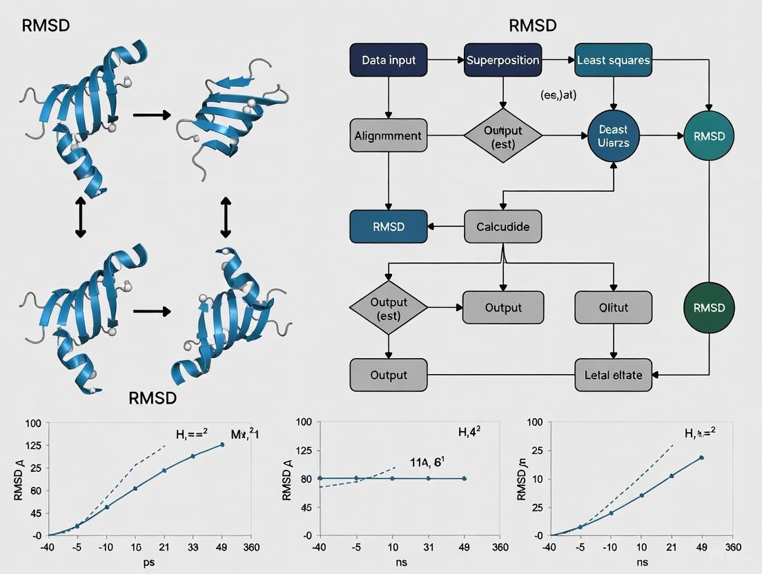
The computational process for calculating RMSD between molecular structures involves a defined sequence of operations, illustrated below:

Figure 1: RMSD Calculation Workflow for Molecular Structures

The roto-translational superposition step (also known as the Kabsch algorithm) is critical for ensuring that RMSD measures internal structural differences rather than arbitrary orientation effects. This algorithm finds the optimal rotation and translation that minimizes the RMSD between two sets of points [8].

RMSD Variants and Normalization

Normalized RMSD for Comparative Analysis

To facilitate meaningful comparisons across different datasets or molecular systems, several normalized RMSD variants have been developed:

• Normalized RMSD (NRMSD): NRMSD = RMSD / (y_max - y_min) where ymax and ymin represent the range of observed values [1].
• Mean-Normalized RMSD: NRMSD = RMSD / ȳ where ȳ is the mean of the measured data [1].
• IQR-Normalized RMSD: RMSD/IQR = RMSD / (Q3 - Q1) where Q1 and Q3 are the first and third quartiles, making the metric less sensitive to extreme values [1].
• Coefficient of Variation of RMSD: CV(RMSD) = RMSD / ȳ which expresses the deviation relative to the mean value [1].

Specialized RMSD Variants in MD

Different research contexts have spawned specialized RMSD implementations:

• Ensemble-Average Pairwise RMSD: Used to quantify global structural diversity in macromolecular ensembles, mathematically related to experimental B-factors [8].
• Backbone RMSD: Calculated using only backbone atoms (C, Cα, N) to focus on protein fold maintenance.
• Ligand RMSD: Specifically measures the deviation of small molecule ligands in binding pockets.
• Residue-Specific RMSD: Calculated per residue to identify local regions of structural variability.

RMSD Calculation Methodologies in MD Validation

Standard MD Validation Protocol

Validating molecular dynamics simulations using RMSD involves a systematic experimental approach:

• Reference Structure Selection: Obtain high-resolution experimental structures (typically from X-ray crystallography or NMR) as reference conformations [3].
• Trajectory Preparation: Process MD simulation trajectories to ensure consistent atom naming, residue numbering, and periodic boundary condition handling.
• Structural Alignment: Perform least-squares fitting of MD snapshots to the reference structure using backbone or specific atom selections to eliminate global translation and rotation [8].
• RMSD Calculation: Compute RMSD values for each trajectory frame relative to the reference structure.
• Time-Series Analysis: Plot RMSD as a function of simulation time to assess equilibration and stability.
• Statistical Analysis: Calculate distributional properties of RMSD values and compare against known benchmarks.

Advanced Clustering Protocols

For complex conformational ensembles, RMSD-based clustering provides enhanced analytical capabilities:

Figure 2: RMSD-Based Clustering for Conformational Analysis

Spectral clustering using RMSD as a distance metric has proven particularly effective for identifying meta-stable and transitional conformations in MD trajectories [6]. This approach involves computing pairwise RMSD between all structures, followed by spectral decomposition of the similarity matrix and k-means clustering in eigenvector space.

Comparative Experimental Data

Performance Across Protein Systems

RMSD values demonstrate variable performance across different protein systems and simulation conditions:

Table 1: RMSD Performance Across Different Protein Systems

Protein System	Residues	Simulation Time	Minimum RMSD (Å)	Application Context
Trp-cage	20	200 ns	<2.0	Folding simulations [4]
Chignolin	10	200 ns	<2.0	Folding simulations [4]
CLN025	10	200 ns	<2.0	Folding simulations [4]
Engrailed Homeodomain	54	200 ns	~1.1*	Native state dynamics [3]
RNase H	155	200 ns	~1.1*	Native state dynamics [3]
Crambin	46	2000 ns	>2.0	Small protein prediction [4]

*Estimated from ensemble-average pairwise RMSD derived from B-factors [8]

Force Field and Software Comparison

Different MD software packages and force fields yield variations in RMSD profiles despite similar overall performance:

Table 2: RMSD Performance Across MD Software and Force Fields

Software Package	Force Field	Water Model	RMSD Profile Characteristics	Experimental Agreement
AMBER	ff99SB-ILDN	TIP4P-EW	Reproduces native state well; samples unfolding at high temperature	Good overall [3]
GROMACS	ff99SB-ILDN	Varies	Similar to AMBER with subtle differences in conformational sampling	Good overall [3]
NAMD	CHARMM36	Varies	Native state dynamics comparable; may resist unfolding at high temperature	Good overall [3]
ilmm	Levitt et al.	Varies	Distinct conformational distributions despite similar experimental agreement	Good overall [3]

Research Reagent Solutions

Essential computational tools and resources for RMSD analysis in MD validation:

Table 3: Essential Research Reagents for RMSD Analysis

Research Reagent	Type	Function in RMSD Analysis	Example Applications
MD Software Packages	Software Suite	Provides algorithms for trajectory integration and basic analysis	AMBER, GROMACS, NAMD, ilmm [3]
Force Fields	Parameter Set	Defines potential energy functions governing simulated dynamics	AMBER ff99SB-ILDN, CHARMM36, Levitt et al. [3]
Solvation Models	Physical Model	Represents solvent effects on protein dynamics	TIP4P-EW, SPC, TIP3P [3]
Analysis Tools	Software Library	Computes RMSD and related metrics from trajectories	MDAnalysis, MDTraj, Bio3D, CPPTRAJ
Clustering Algorithms	Computational Method	Identifies conformational states from RMSD matrices	Spectral clustering, k-means, hierarchical [6]
Validation Databases	Structural Database	Provides reference structures for RMSD comparison	Protein Data Bank (PDB) [4]

RMSD provides a mathematically rigorous foundation for validating molecular dynamics simulations against experimental data. Its calculation framework, incorporating roto-translational superposition and normalization, enables quantitative assessment of structural accuracy across diverse biomolecular systems. While RMSD values under 1.0-2.0 Å typically indicate high structural fidelity, interpretation must consider system size, simulation duration, and research context.

The continued development of normalized RMSD variants and specialized implementations addresses specific challenges in comparative analysis across different molecular systems. When integrated with clustering approaches and complementary validation metrics, RMSD forms an essential component of comprehensive MD validation protocols, providing researchers and drug development professionals with critical insights into the reliability and interpretability of molecular simulations.

Root Mean Square Deviation (RMSD) is a foundational metric in structural biology and computational chemistry, serving as a quantitative measure of the average distance between the atoms of superimposed molecular structures [9]. In the context of molecular dynamics (MD) simulations, RMSD provides a crucial time-dependent measure of conformational change, typically calculated by comparing atomic positions in simulation frames to a reference structure (often the starting crystal structure) [10] [11]. For researchers and drug development professionals, interpreting RMSD values correctly is paramount for assessing simulation stability, determining when a system has reached equilibrium, and validating the reliability of generated structural ensembles. Despite its widespread use, a proper understanding of what the numerical values signify—and what they do not—requires careful consideration of the context, the system under study, and the limitations inherent to this single-metric approach.

This guide examines RMSD interpretation through a critical lens, comparing its utility against alternative metrics and providing structured frameworks for its application within robust MD validation protocols. We present quantitative reference data, detailed methodological protocols for proper RMSD analysis, and visual workflows to guide researchers in avoiding common interpretive pitfalls. By situating RMSD within a broader suite of validation tools, we aim to establish a more nuanced and effective protocol for MD simulation analysis that leverages RMSD's strengths while mitigating its documented weaknesses through complementary approaches.

Quantitative RMSD Interpretation: A Reference Guide

The numerical value of RMSD, expressed in Ångströms (Å), quantifies the magnitude of atomic displacement. However, its interpretation is highly context-dependent, varying with the system studied, the atoms selected for calculation, and the simulation timeframe. The following table synthesizes practical guidelines for interpreting these values across common scenarios.

Table 1: Practical Interpretation Guide for RMSD Values

RMSD Value Range (Å)	Typical Interpretation	Common Context	Recommended Action
0 - 1.0	Very high similarity; minimal fluctuation	• Backbone atoms of a stable, folded protein during production MD.• Comparison of nearly identical crystal structures.	Often indicates a stable, equilibrated system. Proceed with analysis.
1.0 - 2.0	Moderate deviation; common for flexible loops/side chains.	• Backbone of a well-folded protein after equilibration.• Global backbone RMSD for a stable protein-ligand complex.	Represents a typical equilibrium for many proteins. Generally acceptable.
2.0 - 3.0	Significant structural deviation.	• Large-scale domain movements or flexible proteins.• A protein-ligand complex with some ligand mobility.	Investigate the source (e.g., specific domains). Check with other metrics.
> 3.0	Major structural rearrangement or potential instability.	• Global unfolding or large conformational transitions.• A poor-quality model or failed simulation.	Scrutinize simulation parameters and stability. Do not use for analysis without validation.

Beyond these general ranges, specific thresholds are often applied:

• Protein-Ligand Complex Stability: A stable complex typically maintains an RMSD below 2.0 - 3.0 Å [12] [13].
• Model Quality Assessment: In molecular docking, a successful prediction against a known experimental structure often has a heavy-atom RMSD of the ligand below 2.0 Å [13].
• Native State Fluctuations: For a folded protein, the backbone (Cα) RMSD relative to the native state during a simulation is expected to plateau below 2 - 3 Å, though this is highly system-dependent [3].

A critical caveat is that a low RMSD does not guarantee a correct or converged simulation, nor does a high RMSD always indicate a failure; it may represent a valid large-scale conformational change [10] [14]. The following diagram illustrates the core workflow for calculating and interpreting RMSD, highlighting key decision points.

Limitations of RMSD and Complementary Metrics

While RMSD is an intuitive and easily calculated metric, reliance on it as a sole measure of simulation quality is strongly discouraged. A seminal study demonstrated that visual inspection of RMSD plots is a highly subjective and unreliable method for determining system equilibrium, with scientist participants showing no mutual consensus and their judgments being severely biased by plot scaling and color [10]. The core limitations of RMSD are summarized in the table below.

Table 2: Key Limitations of RMSD and Complementary Metrics

Limitation of RMSD	Description	Recommended Complementary Metric
Global Average Masking Local Changes	A low global RMSD can hide significant local fluctuations or functionally important conformational changes in specific regions (e.g., active sites) [14].	Root Mean Square Fluctuation (RMSF): Measures per-residue fluctuation over time, identifying flexible regions [9] [13].
Sensitivity to Outliers	The RMSD value is dominated by the largest deviations (e.g., a single unfolded terminal tail), which can misrepresent the stability of the structural core [14].	Superimposition-Independent Measures: Methods like GDT (Global Distance Test) or Contact-Based Measures are more robust to local errors [14].
Lack of Functional Insight	RMSD quantifies geometric change but provides no direct information about the stability or quality of functionally critical interactions, like hydrogen bonds or binding interfaces.	Hydrogen Bond Analysis & Secondary Structure Count: Tracks the formation and breaking of key molecular interactions and the persistence of structural elements [13].
Dependence on Superposition	The minimal RMSD is found via optimal rigid-body superposition, which can be ambiguous and is often compromised by a small number of deviating fragments [14].	Fit-Free Methods: For example, calculating RMSD based on internal distances (e.g., gmx rmsdist [11]) avoids superposition entirely.

The relationship between RMSD and these complementary metrics within a robust validation protocol is shown in the following workflow.

Experimental Protocols for RMSD Analysis

Protocol: Determining System Equilibration Using RMSD

Determining the point at which a simulation transitions from the initial equilibration phase to a stable production run is a critical step. The following protocol, which avoids reliance on subjective visual inspection, should be applied:

• Data Preparation: Calculate the RMSD for all simulation frames relative to the initial minimized and solvated starting structure. The RMSD is typically calculated for the protein backbone atoms (N, Cα, C) after a least-squares fit to the reference structure to remove global translation and rotation [11].
• Block Averaging: Divide the RMSD time series into sequential, non-overlapping blocks (e.g., 1-nanosecond blocks). Calculate the average RMSD value for each block.
• Statistical Comparison: Compare the average RMSD of the first block to subsequent blocks using a statistical test (e.g., a t-test). The system can be considered equilibrated at the start of a block whose average RMSD is not statistically significantly different (p > 0.05) from the average of the following several blocks.
• Validation: Discard all trajectory frames before the identified equilibration point from subsequent production analysis.

Protocol: Validating Simulations Against Experimental Data

Robust validation requires moving beyond internal metrics (like RMSD) and comparing simulation results with experimental observables [3] [15].

• Generate a Structural Ensemble: Use production-run frames from the equilibrated simulation to create an ensemble of structures representing the simulated conformational landscape.
• Calculate Experimental Observables: Use forward models (computational tools that predict experimental readings from atomic coordinates) to back-calculate experimental data from the simulation ensemble. Common examples include:
  • NMR Observables: Chemical shifts, J-couplings, and Nuclear Overhauser Effect (NOE) data [15] [16].
  • SAXS/SANS: Small-angle X-ray or neutron scattering profiles [15].
  • FRET Efficiencies: For single-molecule Förster resonance energy transfer studies [15].
• Quantitative Comparison: Compare the back-calculated observables to the actual experimental data. A strong agreement, quantified by low RMSD between calculated and experimental values or high correlation coefficients, significantly increases confidence in the simulation's accuracy [3] [16]. Disagreement may indicate issues with the force field, sampling, or both.

The Scientist's Toolkit: Essential Research Reagents & Solutions

The following table details key software, force fields, and analysis tools that form the foundation of modern RMSD analysis and MD simulation validation.

Table 3: Essential Research Reagents and Solutions for MD Analysis

Tool / Reagent	Type	Primary Function in Analysis	Key Consideration
GROMACS [10] [11]	MD Software Package	High-performance simulation engine with built-in tools (gmx rms, gmx rmsf) for trajectory analysis, including RMSD.	Known for its computational speed and extensive analysis suite.
AMBER [10] [3]	MD Software Package	Suite for MD simulation and analysis, incorporating the AMBER force fields.	Widely used for proteins and nucleic acids; includes advanced sampling.
CHARMM36 [3]	Force Field	A set of parameters defining atomic interactions; critical for simulation accuracy.	Results can vary between MD packages even with the same force field [3].
ff99SB-ILDN [3]	Force Field	A variant of the AMBER force field optimized for proteins.	Often used with AMBER and GROMACS packages.
SSM [9]	Structural Alignment Tool	Performs rapid protein structure comparison and superposition.	Used for finding optimal alignment before RMSD calculation.
LGA [14]	Structural Alignment Algorithm	Used in CASP for model evaluation; provides robust local-global alignment.	Less sensitive to local errors than RMSD-minimizing superposition.
CHEMICAL PROBING [15]	Experimental Technique	Provides data on solvent accessibility and base-pairing in RNA, used to inform or validate simulations.	Data can be integrated as restraints in simulations.

RMSD remains an indispensable, if imperfect, tool in the computational scientist's arsenal. Its value lies not in standalone interpretation but in its integrated use within a rigorous, multi-faceted validation protocol. Effective analysis requires understanding that a "good" RMSD value is system-dependent, recognizing the metric's propensity to be biased by outlier fluctuations, and acknowledging the profound subjectivity of visual plateau identification. By supplementing RMSD with local fluctuation analysis (RMSF), interaction monitoring, and—most importantly—validation against experimental data, researchers can move beyond qualitative guesses to achieve quantitative confidence in their molecular dynamics simulations. This disciplined approach is fundamental to producing reliable, reproducible computational insights that can effectively guide drug development and basic research.

In the fields of structural biology and computational biophysics, the quantitative assessment of protein structure and dynamics is fundamental to understanding function, interaction, and stability. Among the most critical metrics for this evaluation are the Root Mean Square Deviation (RMSD) and the Root Mean Square Fluctuation (RMSF). While both metrics originate from the same mathematical concept of measuring spatial differences in atomic positions, they serve distinct purposes and provide complementary information about protein behavior. RMSD quantifies global structural changes over time by comparing atomic coordinates to a reference structure, whereas RMSF measures local flexibility of individual residues throughout a simulation trajectory. For researchers employing Molecular Dynamics (MD) simulations, particularly in drug development where understanding target flexibility and binding stability is crucial, recognizing the appropriate context for each metric is essential for accurate interpretation and validation of computational results. This guide provides a detailed comparison of RMSD and RMSF, including their mathematical definitions, distinct applications, experimental protocols, and interpretation frameworks to enhance the rigor of MD simulation analysis.

Core Concepts and Mathematical Definitions

Root Mean Square Deviation (RMSD)

RMSD is a numerical measurement that represents the average distance between the atoms of two superimposed molecular structures. It is most commonly used to quantify the global structural similarity between a target structure and a reference structure, often the starting conformation of a simulation. The fundamental equation for calculating RMSD between two sets of atomic coordinates is as follows:

• Equation: For two sets of ( n ) vectors representing atomic positions, ( v ) and ( w ), the RMSD is calculated as: [ \mathrm{RMSD} (v, w) = \sqrt{\frac{1}{n} \sum{i=1}^{n} \| vi - wi \|^2 } = \sqrt{\frac{1}{n} \sum{i=1}^{n} ((v{ix} - w{ix})^2 + (v{iy} - w{iy})^2 + (v{iz} - w{iz})^2 )} ] [9]

• Units: RMSD values are expressed in units of length, typically Ångströms (Å), where 1 Å equals (10^{-10}) m [9].

• Application Context: In MD simulations, RMSD is typically calculated after performing a rigid body superposition (translation and rotation) that minimizes the RMSD value between the current frame and the reference structure. This minimization ensures that the measurement reflects internal conformational changes rather than overall molecular translation or rotation [9].

Root Mean Square Fluctuation (RMSF)

RMSF quantifies the deviation of a particle (atom or group of atoms) from its average position over time. Instead of measuring global change relative to a fixed reference, it measures local flexibility around a mean equilibrium position.

• Equation: For a particle ( i ) with coordinate vector ( ri ) over ( T ) frames in a trajectory, where ( \bar{r}i ) is its ensemble average position, the RMSF is calculated as: [ \mathrm{RMSF}(i) = \sqrt{\frac{1}{T} \sum{t=1}^{T} \left( ri(t) - \bar{r}_i \right)^2 } ] [17]

• Units: Like RMSD, RMSF is expressed in Ångströms (Å) [9] [17].

• Application Context: RMSF is particularly valuable for identifying flexible and rigid regions within a protein structure, such as mobile loops, flexible termini, or rigid secondary structure elements like alpha-helices and beta-sheets [18] [13]. When a system fluctuates about a well-defined average position, the RMSD from this average over time can be referred to specifically as the root mean square fluctuation [9].

Table 1: Fundamental Characteristics of RMSD and RMSF

Feature	RMSD	RMSF
Reference Point	Fixed reference structure (e.g., initial frame)	Average structure over the trajectory
Scope of Measurement	Global, system-wide deviation	Local, per-residue or per-atom fluctuation
Primary Information	Overall structural stability/convergence	Local flexibility and mobility patterns
Typical Plot	RMSD vs. Time	RMSF vs. Residue Number
Sensitivity to Fitting	High (requires structural alignment)	Lower (calculated after alignment)

Key Differences and Comparative Applications

Information Content and Analytical Interpretation

The core distinction between RMSD and RMSF lies in the spatial scale of the information they provide, which dictates their respective applications in MD analysis.

• RMSD as a Global Stability Metric: RMSD provides a single value per trajectory frame that reflects the overall structural evolution of the molecule. A time-series plot of RMSD is used to assess if a simulation has reached equilibrium—indicated when the RMSD value plateaus and fluctuates around a stable average [18] [13]. For example, in protein folding simulations, RMSD can serve as a reaction coordinate to quantify the protein's position between the folded and unfolded states [9]. A leveling off of the RMSD curve indicates that the protein has equilibrated [18].

• RMSF as a Local Flexibility Map: RMSF produces a value for each residue or atom, generating a profile of regional flexibility across the protein sequence. This is crucial for identifying functionally important mobile regions, such as flexible loops involved in binding or allosteric regulation [18] [13]. Peaks in the RMSF plot correspond to highly dynamic regions, while low values indicate structural rigidity [19] [13].

Practical Applications in Drug Discovery and Validation

In pharmaceutical research, both metrics offer valuable, non-overlapping insights for target characterization and validation.

• Binding Mode and Complex Stability (RMSD): RMSD is frequently used to assess the stability of a protein-ligand complex in docking and MD simulations. A low RMSD for the protein backbone or the ligand's heavy atoms relative to a reference complex structure suggests a stable, reliable binding pose [13].

• Binding Site and Allosteric Region Analysis (RMSF): RMSF helps identify flexible residues near binding pockets. Changes in RMSF upon ligand binding can indicate conformational selection or induced fit mechanisms [13]. Furthermore, RMSF can pinpoint allosteric sites—distant regions with high flexibility that may influence active site dynamics [20].

Table 2: Application Contexts for RMSD and RMSF in Research

Research Goal	Primary Metric	How it Informs the Analysis
Simulation Equilibration	RMSD	Convergence is signaled by a plateau in the RMSD-time plot.
Protein Thermostability	RMSF	Identifies highly fluctuating residues that may be mutation targets for stabilizing proteins [21].
Ligand Docking Validation	RMSD	Quantifies how closely a predicted binding pose matches an experimental structure.
Understanding Functional Dynamics	RMSF	Reveals flexible loops and termini critical for function and molecular recognition.
Comparing Simulation Ensembles	Both	RMSD checks global structural alignment; RMSF compares local flexibility profiles.

Experimental Protocols and Workflows

Standard Protocol for RMSD Calculation and Analysis

A typical workflow for calculating and interpreting RMSD in an MD simulation trajectory involves the following steps, which can be implemented using tools like cpptraj (AMBER) or MDTraj (Python):

• Trajectory Preparation: Load the simulation trajectory and the corresponding topology file (e.g., .prmtop in AMBER) [18].
• Atom Selection: Select the atoms for the RMSD calculation. For analyzing protein backbone stability, a common mask is @C,CA,N which selects the backbone C, Cα, and N atoms [18].
• Structural Alignment: For each frame in the trajectory, perform a rotational and translational fit (superposition) of the selected atoms onto the same atoms in a reference structure (commonly the first frame). This step removes global translation and rotation, ensuring the RMSD reflects internal conformational changes [9] [18].
• Calculation: Compute the RMSD for the aligned coordinates using the standard equation [9].
• Visualization and Analysis: Plot the RMSD as a function of time (simulation frame) to assess equilibration and structural stability.

The following workflow diagram illustrates this process:

Standard Protocol for RMSF Calculation and Analysis

The protocol for RMSF emphasizes calculating fluctuations relative to an average structure, typically after alignment to remove global motion.

• Trajectory Alignment: First, align the entire trajectory (e.g., using the protein backbone) to a reference frame to remove global rotation and translation. This is a critical step to ensure RMSF reflects internal fluctuations rather than the drift of the entire molecule [18] [17].
• Generate Average Structure: Calculate the time-averaged positions for all atoms, creating an average structure from the aligned trajectory.
• Calculate Fluctuations: For each residue or atom, compute the RMSF using the standard equation, measuring the deviation of its position in each frame from its position in the average structure [17].
• Visualization and Analysis: Plot the RMSF value for each residue against the residue number. High RMSF peaks can be mapped onto the 3D protein structure to visualize spatially flexible regions.

The following workflow diagram illustrates this process:

ExamplecpptrajInput for RMSF

The following is an example input script for the cpptraj module (from AMBER) to calculate RMSF, demonstrating a practical implementation:

Script Explanation:

• trajin: Specifies the input trajectory file.
• rmsd @C,CA,N first: Aligns each frame to the first frame based on the backbone atoms (C, Cα, N).
• atomicfluct ... byres: Calculates the RMSF and outputs it to a file (rmsf_analysis.dat), with results averaged by residue (byres) [18].

The Scientist's Toolkit: Essential Research Reagents and Software

Successful calculation and interpretation of RMSD and RMSF rely on a suite of software tools and theoretical models. The following table catalogues key resources used in the field.

Table 3: Essential Research Tools for RMSD/RMSF Analysis

Tool Name	Type	Primary Function	Relevance to RMSD/RMSF
AMBER (cpptraj) [18] [3]	Software Suite	MD simulation and trajectory analysis	Industry-standard for calculating RMSD, performing alignment, and computing RMSF via scripts.
GROMACS [3] [13]	Software Suite	MD simulation package	Includes built-in tools (gmx rms and gmx rmsf) for efficient calculation of both metrics.
CHARMM [3]	Software Suite	MD simulation and analysis	Provides comprehensive functionalities for dynamics simulation and trajectory analysis.
MDTraj [18]	Python Library	MD trajectory analysis	Enables RMSD/RMSF calculation within customizable Python scripts for integrated analysis workflows.
Elastic Network Models [21] [17]	Theoretical Model	Coarse-grained normal mode analysis	Used in programs like Vibe to calculate residue fluctuations and classify residue mobility [21].
Jmol [20]	Software	Molecular visualization	Visualizes RMSF data by coloring 3D protein structures according to residue fluctuation levels.
PreFRP Web Server [20]	Online Tool	Prediction of fluctuation residues	Classifies residues into high, moderate, and weak fluctuating categories based on sequence and structure.

Data Interpretation Guidelines and Limitations

Guidelines for Interpreting Results

• Benchmarking RMSD Values: There is no universal "good" RMSD value, as it depends on the system and simulation time. However, for stable, folded proteins, backbone RMSD values under 2.0-3.0 Å often indicate a stable simulation. Larger deviations may suggest significant conformational changes or partial unfolding [21].
• Contextualizing RMSF Profiles: Interpret RMSF peaks by mapping them to protein secondary structure. Loops and termini naturally have higher RMSF, while core secondary elements should have lower values. Sudden, sharp peaks might indicate local instability, while broad regions of high fluctuation could relate to domain motions or intrinsic disorder [21] [20].
• Correlation with Experimental Data: RMSF values can be qualitatively compared to crystallographic B-factors (Debye-Waller factors), which also measure atomic displacement [21] [8]. However, discrepancies can arise as B-factors incorporate both dynamic disorder and static crystal packing effects [21].

Common Pitfalls and Limitations

• RMSD Oversimplification: RMSD is a global average and can mask significant local structural changes. A low RMSD does not guarantee that all regions of the protein are stable; localized fluctuations may cancel each other out in the calculation [19].
• Alignment Dependence: The accuracy of RMSD is highly sensitive to the quality of the structural alignment prior to calculation. Improper fitting can lead to artificially inflated RMSD values [9] [17].
• Sampling Time Dependence: Both RMSD and RMSF require sufficient simulation time for convergence. Atomic positional fluctuations may not converge even on a nanosecond timescale for some proteins, and cross-correlations take even longer [22]. Short simulations may not capture rare but important large-scale fluctuations.
• Force Field and Parameter Sensitivity: The absolute values of RMSD and RMSF can be sensitive to the choice of force field, water model, and other simulation parameters, making direct comparisons between studies using different setups challenging [3].

The Critical Role of Reference Structures in RMSD Analysis

In the realm of molecular dynamics (MD) simulations, the Root-Mean-Square Deviation (RMSD) serves as a fundamental metric for quantifying conformational changes and assessing structural stability. RMSD measures the average distance between atoms of superimposed molecular structures, providing a single value that reflects the degree of spatial deviation between two conformations [14]. The calculation involves optimal rigid body superposition followed by measurement of the positional differences of equivalent atoms, typically Cα atoms for protein backbone comparisons [23]. Despite its mathematical simplicity, the interpretation of RMSD values is deeply nuanced, hinging critically on the selection of an appropriate reference structure. This reference choice fundamentally dictates the biological meaning of the resulting RMSD value, transforming the same numerical result from insignificant to critically important depending on the scientific question being addressed.

The critical importance of reference structures stems from the inherent dynamic nature of biomolecules. Proteins and nucleic acids exist not as static entities but as dynamic ensembles sampling multiple conformational states [3] [14]. When comparing three-dimensional structures of globular proteins, two conformers are considered intrinsically similar if their RMSD is smaller than that when one structure is mirror-inverted, establishing a self-referential standard for structural similarity [23]. This article examines the pivotal role of reference structure selection in RMSD analysis, providing comparative data, methodological protocols, and analytical frameworks to enhance the rigor and biological relevance of MD simulation validation.

Comparative Analysis of Reference Structure Impact

Quantitative RMSD Variations Across Reference Types

Table 1: RMSD Values Achieved Using Different Reference Structures in MD Simulations

Protein System	Number of Residues	Reference Structure Type	Simulation Time (ns)	Minimum RMSD (Å)	Key Findings
Trp-cage	20	Experimental (PDB: 1L2Y)	200	<2.0	Structure close to experimental reference achieved [24]
Chignolin	10	Experimental (PDB: 1UAO)	200	<2.0	Near-native structures sampled during simulation [24]
Chignolin	10	Experimental (PDB: 1UAO)	2000	<1.0	Extended simulation improved convergence to reference [24]
HCV Core Protein	191	De novo prediction (AF2)	-	Variable	MD refinement improved initial models; reference quality crucial [25]
RNase H	155	Experimental (PDB: 2RN2)	200	~1.5-3.0	Force-field dependent variations from reference [3]
Engrailed Homeodomain	54	Experimental (PDB: 1ENH)	200	~1.0-2.5	Package-dependent deviations from reference [3]
RNA Models (CASP15)	Various	High-quality starting models	10-50	Modest improvement	MD provided modest improvements for already-good references [26]
RNA Models (CASP15)	Various	Poor starting models	10-50	Often deteriorated	Poor references rarely benefited regardless of simulation length [26]

The selection of reference structure profoundly influences RMSD interpretation and the resulting biological conclusions. Research demonstrates that for small proteins (10-46 residues), MD simulations can achieve RMSD values below 2.0 Å when using experimental structures as references, with Trp-cage (20 residues) achieving particularly close correspondence to its experimental reference within 200 ns simulations [24]. However, the minimum RMSD values alone do not guarantee that simulations converge to the reference structure, as the conformations closest to experimental references often occurred transiently during simulations rather than at their endpoints [24].

For larger and more complex systems, the relationship between reference structure quality and RMSD outcomes becomes increasingly critical. In studies of the hepatitis C virus core protein (HCVcp), where experimental structures remain unavailable, researchers utilized de novo prediction tools (AlphaFold2, Robetta, trRosetta) and template-based approaches (MOE, I-TASSER) to generate reference structures [25]. Subsequent MD simulations served to refine these models, with the initial reference quality directly determining the extent of improvement possible. Similarly, in RNA structure prediction, MD simulations provided modest improvements for high-quality starting models but often deteriorated poorly-predicted references, regardless of simulation length [26].

Methodological Considerations for Reference Selection

Table 2: Advantages and Limitations of Reference Structure Types

Reference Type	Typical Applications	Advantages	Limitations	Representative RMSD Range
Experimental (X-ray, NMR, Cryo-EM)	Native state stability, Folding validation	High experimental accuracy, Standard for validation	Static snapshot, May miss dynamics, Crystal packing artifacts	1-3 Å for well-folded proteins [24] [3]
De novo Predicted Models	Proteins lacking experimental structures	Availability, Completeness	Variable accuracy, Force field biases	Highly variable (quality-dependent) [25]
Starting Structure	Equilibration monitoring, Simulation stability	Direct measure of conformational drift	Does not reflect biological accuracy	Typically decreases during equilibration [3]
Average Structure from Ensemble	Characterizing native state fluctuations	Represents ensemble behavior, Reduces noise from outliers	Computation-intensive, May obscure transitions	~0.5-1.5 Å for stable folded proteins [3]
Alternative Experimental Conformers	Functional studies, Allosteric mechanisms	Captures biological relevance, Functional insights	May represent different thermodynamic states	1-4 Å for functionally distinct states [14]

The choice of reference structure must align with the specific research question. For studies of native state stability and folding, experimental structures serve as indispensable references, providing an objective standard for assessing structural conservation [24]. When experimental references are unavailable, as with many membrane proteins or novel designed proteins, de novo predicted models offer alternatives but introduce additional uncertainty into RMSD interpretation [25]. For functional studies investigating conformational changes, alternative experimental structures representing different states (e.g., active/inactive conformations) provide more biologically relevant references than a single static structure [14].

The limitations of RMSD as a global metric necessitate careful reference selection. Because RMSD is dominated by the largest structural errors and can be heavily influenced by flexible regions, a reference structure that appropriately represents the biological question is essential [14]. For example, in multi-domain proteins with relative domain movements, using a reference structure that captures the relevant biological state prevents misinterpretation of domain motions as structural instability [14].

Experimental Protocols for RMSD Analysis

Standardized Workflow for RMSD Calculation

The RMSD calculation workflow begins with critical decisions regarding reference selection based on research objectives. The mathematical foundation for RMSD calculation follows the formula:

RMSD = √[1/n × Σ(d_i)²]

where n represents the number of atom pairs, and di is the distance between the i-th pair of equivalent atoms after optimal superposition [14] [27]. For a molecular structure represented by Cartesian coordinate vector ri of N atoms, the RMSD is calculated with respect to a reference structure with coordinates r_i⁰, incorporating a transformation matrix U that defines the best-fit alignment between structures along trajectories [27].

Advanced Protocol for Multi-Reference Analysis

For complex systems exhibiting multiple conformational states, a single reference structure often proves insufficient. In such cases, researchers should implement a multi-reference RMSD analysis protocol:

• Identify biologically relevant conformers from experimental databases or previous simulations
• Calculate RMSD time series against each reference conformation
• Apply clustering algorithms to identify predominant conformational states
• Construct probability distributions of RMSD values for each state
• Implement state assignment algorithms based on RMSD thresholds

This approach proved particularly valuable in studies of TEM-1 β-lactamase, where researchers employed random forest classification based on pairwise Cα distances to differentiate functional states, demonstrating that residue-specific importance in distinguishing states could be quantified and mapped [27]. Such multi-reference frameworks transform RMSD from a simple stability metric into a powerful tool for characterizing conformational landscapes and functional transitions.

Complementary Validation Metrics

Table 3: Complementary Metrics for Comprehensive Structural Validation

Analytical Metric	Computational Formula	Structural Feature Assessed	Complementary Role to RMSD
Root-Mean-Square Fluctuation (RMSF)	RMSF = √[1/T × Σ(ri(t) - rī)²] [27]	Per-residue flexibility	Identifies localized flexibility that global RMSD may obscure
Radius of Gyration (Rg)	Rg = √(1/M × Σmi × ri²)	Global compactness	Assesses overall folding independent of specific reference alignment
Principal Component Analysis (PCA)	Cij = ⟨(ri - rī) • (rj - r_j̄)⟩ [27]	Collective motions	Identifies dominant conformational sampling patterns
Solvent Accessible Surface Area (SASA)	-	Surface exposure	Probes burial of hydrophobic cores and binding interfaces
Native Contacts	Q = 1/Ncontacts × Σδij	Preservation of specific interactions	Quantifies essential stabilizing interactions directly

While RMSD provides valuable global structural information, comprehensive validation requires integration with complementary metrics that capture different aspects of structural dynamics. Root-Mean-Square Fluctuation (RMSF) measures the fluctuation of individual atoms around their mean positions, effectively identifying flexible regions that may dominate global RMSD values [27] [28]. Principal Component Analysis (PCA) reduces the dimensionality of structural variance, extracting dominant modes of motion from MD trajectories and providing insights into collective motions that may be obscured in simple RMSD analysis [27]. For the human superoxide dismutase (SOD1) system, researchers combined RMSD with radius of gyration, SASA, hydrogen bonding, and essential dynamics to comprehensively characterize structural behavior across multiple crystallographic references [28].

Practical Guidelines and Future Perspectives

The critical role of reference structures in RMSD analysis demands rigorous experimental design and thoughtful interpretation. Researchers should adopt the following best practices:

• Explicitly justify reference selection based on specific research questions and biological context
• Implement multiple reference structures when studying systems with known conformational heterogeneity
• Always report reference structure identifiers (PDB codes, model generation methods) to enable reproducibility
• Contextualize RMSD values with appropriate biological thresholds, recognizing that significance depends on system size, flexibility, and biological question
• Integrate RMSD with complementary metrics to develop a multidimensional view of structural dynamics

The field continues to evolve with emerging methods addressing current limitations. Machine learning approaches, such as the random forest implementation used in TEM-1 studies, offer powerful frameworks for identifying structurally significant residues and classifying conformational states beyond simple RMSD thresholds [27]. Multi-ensemble referencing strategies, which utilize entire experimental ensembles rather than single structures as references, promise more comprehensive assessments of simulation accuracy [3]. As force fields continue to improve and simulation timescales extend, the critical role of appropriate reference selection will only grow in importance for validating MD simulations against experimental reality and extracting biologically meaningful insights from computational structural biology.

The Root Mean Square Deviation (RMSD) is a ubiquitous metric in computational biology for quantifying structural changes in Molecular Dynamics (MD) simulations and docking studies. However, reliance on RMSD as a sole validation measure is fundamentally inadequate for assessing the quality of molecular equilibria or binding poses. This guide objectively compares the performance of various computational methods, demonstrating through experimental data that RMSD values often correlate poorly with physical plausibility, biological relevance, and functional accuracy. A multi-metric validation protocol is essential for robust research outcomes.

The Deceptive Simplicity of RMSD: A Primer

RMSD measures the average distance between the atoms of two superimposed structures, typically comparing a simulated structure to an experimental reference. A low RMSD value (conventionally < 2.0–2.5 Å for ligands, < 1.0–2.0 Å for proteins) is often interpreted as a successful prediction or a stable simulation [29]. While this metric provides a useful global measure of structural deviation, its simplicity belies critical limitations. RMSD is agnostic to critical biochemical details; it cannot distinguish between a physically plausible conformation with correct molecular interactions and a pose with steric clashes, incorrect bond geometries, or missing key interactions. Consequently, an over-reliance on RMSD can lead to the validation of structurally inaccurate or functionally irrelevant models, compromising downstream research and development efforts.

Comparative Performance Data: RMSD vs. Advanced Metrics

Performance Discrepancies in Molecular Docking

A comprehensive benchmark of molecular docking programs revealed a critical divergence between RMSD-based success and physical plausibility. The following table summarizes the performance of selected methods, highlighting this gap.

Table 1: Docking Performance: Pose Accuracy vs. Physical Validity

Docking Method	Method Type	RMSD ≤ 2 Å Success Rate (%)	Physical Validity (PB-Valid) Rate (%)	Combined Success Rate (%)
Glide SP	Traditional	72.94	97.20	71.18
SurfDock	Generative AI	91.76	63.53	61.18
DiffBindFR (MDN)	Generative AI	75.29	58.24	47.65
AutoDock Vina	Traditional	68.24	87.06	61.18
KarmaDock	Regression AI	47.65	25.29	15.88

Source: Adapted from Li et al. (2025), evaluation on the Astex diverse set [30].

The data demonstrates that while AI-based generative models like SurfDock excel at achieving low RMSD values, they frequently generate poses with poor physical validity, including steric clashes and incorrect bond lengths. In contrast, traditional methods like Glide SP maintain high physical plausibility, making them more reliable for applications requiring chemically accurate models, despite a potentially lower top-tier RMSD success rate [30].

Efficacy of MD Refinement for RNA Structures

The limitations of RMSD are further exposed in MD-based refinement of biomolecular structures. A benchmark study from CASP15 on RNA models provides clear experimental evidence.

Table 2: MD Refinement Outcomes for RNA Models Based on Initial Quality

Starting Model Quality	Likelihood of Improvement via Short MD (10-50 ns)	Typical Effect of Long MD (>50 ns)	Recommended Protocol
High-Quality	Modest improvement possible; stabilizes stacking and non-canonical base pairs.	Often induces structural drift and reduces fidelity.	Use short MD for fine-tuning and stability testing.
Poor-Quality	Rarely benefits; often deteriorates.	High probability of significant degradation.	Not recommended; use alternative modeling approaches.

Source: Insights from CASP15 RNA modeling benchmark [26].

This study concluded that MD works best for fine-tuning reliable models and for quickly testing their stability, not as a universal corrective method. The initial model quality, which cannot be assessed by RMSD alone, is the primary determinant of refinement success [26].

Experimental Protocols for Multi-Metric Validation

A Workflow for Comprehensive Docking Validation

To overcome the limitations of RMSD, a multi-dimensional validation protocol is necessary. The following workflow, derived from benchmarking studies, provides a robust framework for evaluating docking predictions [30]:

• Pose Prediction Accuracy: Calculate the RMSD of the docked ligand pose against the crystallographic reference. A pose with RMSD ≤ 2.0 Å is traditionally considered a correct prediction [29].
• Physical Plausibility Check: Use a tool like the PoseBusters toolkit to validate the chemical and geometric consistency of the predicted complex. This checks for correct bond lengths, angles, absence of steric clashes, and proper stereochemistry [30].
• Interaction Recovery Analysis: Perform a residue-specific interaction analysis (e.g., hydrogen bonds, hydrophobic contacts, halogen bonds) to verify that the key interactions observed in the experimental structure are recapitulated in the docked pose.
• Virtual Screening (VS) Efficacy Assessment: Evaluate the method's ability to enrich active compounds over decoys in a virtual screening experiment, typically analyzed using Receiver Operating Characteristic (ROC) curves and the Area Under the Curve (AUC) [29].

Protocol for MD Simulation Validation

For validating MD simulations, particularly for complex systems like proteins and RNA, a similar multi-faceted approach is required:

• Global Stability (RMSD): Monitor the backbone RMSD of the protein/nucleic acid relative to the starting structure to ensure the simulation has stabilized and reached an equilibrium.
• Local Flexibility (RMSF): Calculate the Root Mean Square Fluctuation (RMSF) of individual residues to assess local stability and identify flexible regions. This complements the global picture from RMSD.
• Secondary Structure Conservation: Use algorithms like DSSP to track the conservation of secondary structural elements (α-helices, β-sheets) over the simulation trajectory [5].
• Energetic and Solvation Analysis: Compute the Solvation Free Energy (DGSolv) and monitor interaction energies (Coulombic, Lennard-Jones) to ensure thermodynamic plausibility [31].
• Principal Component Analysis (PCA): Perform PCA to identify the large-scale, collective motions that define the functional conformational landscape, which are often obscured by simple RMSD analysis [5].

The Scientist's Toolkit: Essential Research Reagents & Software

Table 3: Key Computational Tools for Advanced Biomolecular Analysis

Tool Name	Category	Primary Function	Relevance Beyond RMSD
PoseBusters	Validation Toolkit	Checks physical plausibility and geometric correctness of docked poses.	Flags steric clashes and bad bond angles missed by RMSD [30].
GROMACS	MD Simulation Engine	Performs high-performance molecular dynamics simulations.	Enables calculation of RMSF, DSSP, and free energies [31].
Amber	MD Simulation Suite	Simulates biomolecular motion with advanced force fields.	Used with χOL3 for RNA-specific refinement studies [26].
DSSP	Algorithm	Defines protein secondary structure from 3D coordinates.	Tracks stability of helices/sheets during MD simulation [5].
MM-PBSA	Energetics Calculator	Estimates binding free energies from MD trajectories.	Provides thermodynamic validation of interactions [5].
BioEmu	AI Simulator	Generates protein equilibrium ensembles using diffusion models.	Predicts conformational states and free energy distributions [32].

The empirical evidence is clear: RMSD is a necessary but insufficient metric for validating the output of molecular docking and dynamics simulations. Relying on it alone can be misleading, as high-quality models can be incorrectly rejected and physically implausible models accepted. The future of reliable computational biology lies in the adoption of multi-dimensional validation protocols that integrate measures of physical plausibility, chemical interaction fidelity, local stability, and thermodynamic soundness. By moving beyond RMSD, researchers can generate more predictive and biologically relevant computational data, thereby accelerating the pace of discovery in drug development and structural biology.

From Theory to Practice: Executing Robust RMSD Analysis Protocols

Step-by-Step Protocol for RMSD Calculation and Trajectory Alignment

Root Mean Square Deviation (RMSD) is a fundamental metric in structural biology and molecular dynamics (MD) simulations, providing a quantitative measure of conformational change by calculating the average distance between corresponding atoms in two molecular structures after optimal alignment [18] [13]. In MD simulations, RMSD is typically plotted against time to monitor system stability, identify equilibration points, and assess large-scale structural changes as compared to a starting reference structure [18]. For researchers validating MD simulations, RMSD analysis serves as a crucial benchmark for assessing the convergence and quality of simulated trajectories against experimental data [3].

The reliability of MD simulations depends heavily on both sampling adequacy and force field accuracy [3]. While RMSD provides global structural comparison, its proper interpretation requires understanding its relationship with other metrics like Root Mean Square Fluctuation (RMSF), which quantifies local residue flexibility [33] [18]. This protocol establishes standardized methodologies for RMSD calculation and trajectory alignment to enable consistent cross-study comparisons and robust validation of molecular dynamics simulations.

Theoretical Foundations and Relationships

Mathematical Definition of RMSD

The RMSD between two molecular structures is mathematically defined as the square root of the mean squared distance between corresponding atoms after optimal roto-translational alignment:

RMSD = √[ (1/N) × Σᵢ (rᵢ - rᵢ')² ]

Where N represents the number of atoms being compared, rᵢ denotes the position of atom i in the target structure, and rᵢ' represents the position of the corresponding atom in the reference structure after superposition [33]. This calculation requires solving the least-squares problem to find the optimal rotation and translation that minimizes the RMSD value between the two structures.

Relationship Between RMSD, RMSF, and B-Factors

A fundamental relationship exists between ensemble-average pairwise RMSD and experimental B-factors derived from X-ray crystallography. Under conservative assumptions, the root mean-square ensemble-average of an all-against-all distribution of pairwise RMSD for a single molecular species, ) and

RMSFᵢ² = 3Bᵢ/8π² [33]

This relationship enables researchers to quantify global structural diversity of macromolecules in crystals directly from experimental X-ray data, with typical ensemble-average pairwise backbone RMSD for protein x-ray structures approximately 1.1 Å [33]. This correspondence provides a crucial bridge between computational simulations and experimental observables for validation purposes.

Software Tools for RMSD Analysis

Comparative Performance Analysis

Multiple software packages are commonly employed for RMSD analysis in MD simulations, each with distinct algorithms and performance characteristics. Recent benchmarking studies reveal significant variations in conformational sampling and structural outcomes between different MD packages, even when using similar force fields [3].

Table 1: Software Tools for RMSD Calculation and Analysis

Software Tool	Primary Method	Key Features	Alignment Approach	Best Applications
CPPTRAJ [18]	Trajectory analysis	Part of AMBER tools; calculates RMSD, RMSF, H-bonds	Backbone atom fitting (@C,CA,N)	Long MD trajectories; protein dynamics
MDTraj [18]	Python library	Fast RMSD calculation; integration with data science stack	Optimal rotation and translation	Custom analysis scripts; high-throughput processing
PyMOL ColorByRMSD [34]	Visualization script	Colors structures by RMSD; stores values as B-factors	C-alpha atom alignment	Visual comparison; publication figures
jFATCAT [35]	Flexible alignment	Accommodates hinges and twists in structures	Both rigid-body and flexible	Proteins with conformational changes
TM-align [35]	TM-score based	Focus on global topology similarity	Dynamic programming	Fold recognition; distant homologs

Experimental Validation of MD Packages

Comprehensive studies comparing four major MD simulation packages (AMBER, GROMACS, NAMD, and ilmm) revealed subtle but significant differences in conformational distributions and sampling extent, despite overall reproduction of experimental observables [3]. These differences become more pronounced during larger amplitude motions like thermal unfolding, with some packages failing to allow proper unfolding at high temperature or providing results inconsistent with experimental data [3].

Performance variations stem not only from force field differences but also from implementation factors including water models, constraint algorithms, nonbonded interaction treatment, and simulation ensemble employed [3]. This underscores the importance of standardized RMSD protocols to enable meaningful comparisons across different simulation platforms.

Step-by-Step Protocols

RMSD Calculation with MDTraj

MDTraj provides a Python-based approach for efficient RMSD calculation with integration into scientific computing workflows:

This protocol emphasizes using backbone atoms (C, CA, N) for alignment to focus on global protein structural changes while minimizing noise from side chain fluctuations [18].

RMSD Analysis with CPPTRAJ

CPPTRAJ offers a comprehensive command-line approach for advanced trajectory analysis:

Input File Preparation (rmsd_analysis.in):

Execution Command:

CPPTRAJ automatically performs rotational and translational fitting to the reference structure (typically the first frame) before RMSD calculation, eliminating artifacts from whole-molecule diffusion [18]. The "byres" flag enables residue-wise analysis for RMSF calculations that complement global RMSD metrics.

Workflow Diagram for RMSD Analysis

Diagram 1: Comprehensive workflow for RMSD calculation and analysis from MD simulations

Advanced Alignment Methodologies

Rigid-Body Versus Flexible Alignment

Structural alignment algorithms employ different strategies for molecular superposition, each with distinct advantages for specific applications:

• Rigid-Body Alignment: Maintains fixed relative atom positions within each structure, optimizing only global rotation and translation. Methods like jFATCAT-rigid and jCE are ideal for closely related structures with minimal internal flexibility [35].

• Flexible Alignment: Accommodates relative mobility between domains or subdomains through introduced hinges or twists. jFATCAT-flexible enables meaningful comparison of proteins in different conformational states or with distant evolutionary relationships [35].

• Topology-Independent Alignment: CE-CP handles circularly permuted proteins or those with different backbone connectivity while maintaining spatial arrangement of structural elements [35].

Domain-Specific Alignment Strategies

For large proteins or multi-domain systems, global RMSD may obscure localized conformational changes. Domain-based alignment provides more insightful analysis:

This approach proved essential in studies of viral capsid proteins like HCV core protein, where different domains exhibit distinct structural behaviors and functions [25].

Visualization and Interpretation

Color-Coded RMSD Mapping

Visual representation enhances interpretation of RMSD analysis results. PyMOL's ColorByRMSD script enables intuitive visualization:

This script colors structures by local RMSD values using a blue-to-red spectrum, with blue indicating minimal deviation and red indicating maximal deviation [34]. Unaligned regions are colored gray, providing immediate visual identification of variable and conserved structural regions.

Multi-Trajectory Comparison

Comparing multiple simulation replicates or conditions requires consistent alignment and normalization:

This approach facilitates assessment of sampling convergence and reproducibility across independent simulations [18].

Research Reagents and Computational Tools

Table 2: Key Research Reagents and Computational Tools for RMSD Analysis

Tool/Resource	Type	Primary Function	Application in RMSD Analysis
AMBER [3] [18]	MD Package	Molecular dynamics simulations	Generating trajectories for RMSD analysis
GROMACS [3]	MD Package	High-performance MD simulations	Alternative engine for trajectory generation
CPPTRAJ [18]	Analysis Tool	Trajectory analysis	Primary RMSD calculation and processing
MDTraj [18]	Python Library	Molecular analysis	Programmatic RMSD analysis and customization
PyMOL [34]	Visualization	Molecular graphics	Visual representation of RMSD results
RCSB PDB [35]	Database	Experimental structures	Reference structures for alignment validation
Jupyter Notebook [18]	Computing Environment	Interactive analysis	Creating reproducible analysis workflows

Validation and Best Practices

Experimental Correlation

Validating RMSD analysis protocols requires correlation with experimental data. Studies of engrailed homeodomain and RNase H demonstrated that while multiple MD packages reproduced experimental observables equally well overall, subtle differences emerged in conformational distributions and sampling extent [3]. Successful validation strategies include:

• Comparing simulation-derived B-factors with experimental crystallographic B-factors using the relationship RMSFᵢ² = 3Bᵢ/8π² [33]
• Assessing ability to reproduce known conformational changes from experimental structures
• Validating against spectroscopic data such as NMR chemical shifts when available

Troubleshooting Common Issues

• High RMSD Values: May indicate legitimate conformational changes or artifacts from poor alignment. Verify alignment strategy and atom selection.
• RMSD Drift: Continuous increase may suggest incomplete equilibration; extend equilibration phase or check simulation stability.
• Alignment Artifacts: Ensure consistent atom selection across all frames and eliminate translational/rotational degrees of freedom.
• Convergence Assessment: Use multiple replicates and statistical measures to confirm sampling adequacy [3].

Standardized protocols for RMSD calculation and trajectory alignment are essential for robust validation of molecular dynamics simulations. This comprehensive guide establishes reproducible methodologies spanning multiple software platforms while emphasizing experimental correlation and appropriate interpretation. The integration of quantitative RMSD analysis with complementary metrics like RMSF and experimental validation creates a foundation for reliable assessment of structural dynamics in biomedical research.

As MD simulations continue to complement experimental structural biology [3], rigorous RMSD protocols will remain crucial for benchmarking force fields, assessing conformational sampling, and building confidence in simulation-based predictions for drug development and structural biology.

Best Practices for Selecting Atoms and Residues for Analysis

In molecular dynamics simulations, the selection of atoms and residues for analysis represents a fundamental methodological choice that directly impacts the interpretation of protein dynamics, stability, and function. Within the broader context of RMSD analysis protocols for MD simulation validation research, appropriate selection strategies determine whether computational results provide biologically meaningful insights or misleading artifacts. Research demonstrates that even identical proteins analyzed under different selection parameters can yield significantly different RMSD profiles, highlighting the necessity of standardized, validated approaches [36]. This comparison guide objectively evaluates current methodologies, supporting experimental data, and best practices for atomic-level selection in MD analysis across major research applications.

Fundamental Selection Concepts and Terminology

Core Selection Categories

Molecular dynamics analysis packages provide specialized syntax for selecting specific subsets of atoms based on various molecular properties. The most robust selection strategies combine multiple approaches to address specific research questions while maintaining consistency across simulations.

Table 1: Fundamental Atom Selection Categories in MD Analysis

Category	Selection Examples	Primary Applications	Key Considerations
Simple Selections	protein, backbone, nucleic, nucleicbackbone	Rapid assessment of global stability	Protein identification uses hard-coded residue names may not recognize esoteric residues [37]
Property-Based	segid DMPC, resid 1:5, resname LYS, name CA	Targeted analysis of specific regions	Force field dependency for atom names; resid versus resnum distinctions [37]
Geometric	around 3.5 protein, point 5.0 5.0 5.0 3.5, prop z >= 5.0	Binding studies, solvation shells, membrane interactions	Periodicity considerations across simulation boundaries [37]
Boolean Logic	protein and not (resname ALA or resname LYS)	Isolating specific structural elements	Parentheses essential for complex logical groupings [37]
Index-Based	bynum 1:5, index 0:4	Precise atom-level analysis	1-based (bynum) versus 0-based (index) numbering systems [37]

Selection Command Implementation

The MDAnalysis package implements a selection syntax similar to CHARMM's atom selection syntax, providing researchers with a versatile toolkit for constructing precise atomic queries [37]. Selection commands return AtomGroup objects with atoms sorted according to their topology index, ensuring no duplicates appear even in complex selections. For example:

• universe.select_atoms("segid KALP") - Selects all atoms with segment identifier KALP
• universe.select_atoms("segid DMPC and not (name H* or type OW)") - Combines pattern matching with boolean logic
• universe.select_atoms("resid 1:100 and backbone") - Selects backbone atoms from residues 1 to 100

Pattern matching extends selection capabilities using wildcards (*), single character matches (?), and character sequences ([seq]), enabling researchers to target specific chemical environments without exhaustive residue listing [37].

Comparative Analysis of Selection Methodologies

Backbone versus All-Atom Selection for RMSD Analysis

The choice between backbone and all-atom selections for RMSD calculations represents one of the most fundamental methodological decisions in MD validation. Experimental data reveals significant differences in RMSD profiles and interpretation depending on selection strategy.

Table 2: Backbone vs. All-Atom RMSD Selection Comparison

Selection Type	Typical RMSD Range	Structural Sensitivity	Best Applications	Limitations
Backbone (CA, C, N, O)	1-3 Å (stable fold) [24]	Moderate - detects global conformational changes	Protein folding studies, domain movements	May miss side-chain rearrangements critical to function
All Heavy Atoms	1.5-4 Å (stable fold) [3]	High - captures side-chain reorientations	Binding site analysis, allosteric communication	Increased noise from flexible surface residues
Alpha Carbons Only	0.5-2.5 Å (stable fold) [38]	Low - most stable reference	High-level comparison of structural conservation	Limited information about local structural quality

Research demonstrates that backbone RMSD values below 2 Å generally indicate high structural similarity, while values exceeding 3-4 Å suggest significant conformational changes [38]. A study of short test proteins (10-46 residues) found that MD simulations could achieve backbone RMSD values below 2.0 Å compared to experimental structures for proteins up to approximately 20 residues using 200-ns simulations [24]. However, the same study noted that RMSD values fluctuated substantially throughout simulations and structures did not necessarily converge to the experimental conformation by simulation end, highlighting the importance of selection consistency across time-series analysis.

Domain-Specific versus Global Selection Strategies

Targeted selection of specific protein domains or structural elements often provides more biologically relevant insights than global RMSD calculations, particularly for multi-domain proteins or proteins with flexible regions.

In a comprehensive comparison of four MD packages (AMBER, GROMACS, NAMD, and ilmm) analyzing engrailed homeodomain (EnHD) and RNase H, researchers found that domain-specific analysis revealed subtle differences in conformational distributions and sampling extent that were obscured in global RMSD calculations [3]. While overall reproduction of experimental observables was similar across packages, domain-specific motions differed significantly, creating ambiguity about which results most accurately reflected biological reality.

The iGEM UBC team's analysis of fusion proteins for surface display demonstrated the value of combining multiple selection strategies [38]. They employed both RMSD (measuring deviation from reference structure) and radius of gyration (measuring structural compactness) to obtain complementary views of protein stability under different pH conditions. Their findings highlighted how identical selection strategies applied to different fusion protein constructs revealed stability variations critical to experimental design.

Figure 1: Atom Selection Strategy Decision Workflow for MD Analysis

Selection for Specialized Analytical Applications

Ligand-Binding Site Analysis

When analyzing protein-ligand complexes, selection strategies must capture both stability of the binding pocket and ligand interaction dynamics. A forum discussion highlighted that identical proteins complexed with different drugs exhibit different RMSD profiles due to simulation randomness and ligand-specific effects [36]. Researchers recommended comparing complex RMSD both to apo protein structures and to each complex's own starting structure to differentiate ligand-induced stabilization from inherent protein flexibility.

For hydrogen bond analysis in ligand-binding studies, MDAnalysis implements geometric thresholds with default parameters of 3.0 Å for donor-acceptor distance and 120° for donor-hydrogen-acceptor angle [39]. Selection syntax for such analysis typically combines residue and atom specifications, such as (resname LIG and not name H*) to select non-hydrogen atoms of a ligand, enabling precise monitoring of interaction stability.

Fusion Protein and Engineered System Analysis

The iGEM UBC team's investigation of carbonic anhydrase fusion proteins demonstrated specialized selection strategies for engineered systems [38]. They employed structural alignment to examine conformational changes in the enzymatic domain when fused to different surface display proteins (VCBS, INPN, RsaA). Their pipeline selected specifically for the catalytic domain across different fusion contexts, enabling direct comparison of enzymatic function preservation despite varying fusion partners.

This approach highlights how custom selection strategies that target functional domains rather than entire constructs can provide more meaningful validation metrics for engineered protein systems. Their methodology revealed that while global fusion protein structures showed considerable variation, the enzymatic active sites maintained stable configurations with RMSD values below 2Å in optimal constructs.

Experimental Protocols and Validation Frameworks

Standardized Protocol for Selection Validation

Based on comparative analysis of multiple studies, we propose a standardized protocol for validating atom selection strategies in MD analysis:

• Initial Structure Assessment

  • Select backbone atoms (protein and nucleic) for global structure alignment
  • Calculate initial RMSD to reference structure using align.AlignTraj (MDAnalysis) [39]
  • Identify flexible regions via RMSF analysis of Cα atoms

• Domain-Specific Selection

  • Define structural domains based on known topology or clustering analysis
  • Calculate domain-specific RMSD relative to globally aligned trajectory
  • Compare domain motions to identify correlated movements

• Functional Site Isolation

  • Select residues within specific distance (e.g., around 5.0 resname LIG) of functional elements [37]
  • Calculate local RMSD for binding pockets or catalytic sites
  • Monitor specific interactions (hydrogen bonds, hydrophobic contacts)

• Cross-Validation with Experimental Data

  • Compare simulation fluctuations to B-factors from crystallographic data
  • Validate predicted flexible regions against NMR relaxation data
  • Assess functional implications of observed dynamics

This protocol was applied successfully in a study of grancalcin, where researchers combined RMSD, Rg, and RMSF analysis to confirm stable, compact states throughout 100 ns simulations [40]. Their selection of specific domains and comparison to template structures enabled confident interpretation of dynamic properties despite the absence of experimental crystal structures.

Case Study: Multi-Package Validation

A comprehensive evaluation of four MD simulation packages (AMBER, GROMACS, NAMD, and ilmm) provides exemplary methodology for selection strategy validation [3]. Researchers performed triplicate 200-nanosecond simulations of two proteins with distinct topologies using "best practice parameters" established by each package's developers. Their analysis included:

• Backbone RMSD calculations relative to crystal structures
• Domain-specific mobility analysis
• Comparison of conformational distributions across packages
• Validation against diverse experimental data

This study revealed that while overall reproduction of experimental observables was similar across packages, domain-specific motions and conformational sampling differed significantly. These findings underscore the importance of consistent selection strategies when comparing results across different simulation packages or force fields.

Figure 2: Multi-Scale Selection Strategy for Comprehensive MD Validation

The Scientist's Toolkit: Essential Research Reagents and Solutions

Table 3: Essential Tools for Atom Selection and MD Analysis

Tool/Category	Specific Examples	Primary Function	Selection Capabilities
MD Simulation Packages	GROMACS [38], AMBER [3], NAMD [3]	Molecular dynamics engine	Varies by package; GROMACS provides extensive selection syntax
Analysis Toolkits	MDAnalysis [37] [39], MDTraj, VMD	Trajectory analysis and processing	Advanced selection syntax with biological and geometric options [37]
Visualization Tools	PyMOL [38], NGL View [39]	Structural visualization and rendering	Interactive selection of atoms and residues
Structure Prediction	AlphaFold2 [38] [25], Robetta [25], trRosetta [25]	de novo structure prediction	pLDDT confidence metrics guide selection of reliable regions
Validation Databases	PDB [38], SASBDB, BMRB	Experimental structure and dynamics data	Reference data for selection validation

The comparative analysis presented herein demonstrates that atom and residue selection strategies fundamentally influence MD simulation interpretation and validation. Key findings indicate that:

• Multi-scale selection approaches (global, domain-specific, local) provide complementary insights into protein dynamics
• Backbone selections generally offer the most robust metrics for global stability assessment
• Domain-specific analyses reveal functional motions often obscured in global calculations
• Selection consistency is critical for meaningful comparison across simulations and packages
• Validation against experimental data remains essential for selection strategy verification

As MD simulations continue to grow in complexity and application scope, standardized selection methodologies will become increasingly important for ensuring reproducible, biologically relevant conclusions. The protocols and comparisons presented here provide a framework for researchers to implement validated selection strategies in their MD analysis workflows.

Root Mean Square Deviation (RMSD) analysis is a cornerstone protocol for validating Molecular Dynamics (MD) simulations, providing a quantitative measure of conformational changes and simulation stability over time. Within drug discovery and development, ensuring the reliability of MD simulations through rigorous RMSD analysis is paramount, as these simulations provide critical insights into molecular interactions, stability, and dynamics that influence drug design decisions [31]. The convergence of RMSD and other properties is a fundamental indicator that a simulation has sufficiently sampled the conformational space relevant to the biological question at hand [41]. The integration of automated MD software packages with powerful Python scripting libraries has created a powerful paradigm for conducting robust, reproducible, and scalable RMSD analysis. This guide objectively compares the performance and capabilities of prominent MD software and Python tools, providing researchers with the experimental data and methodologies needed to validate their simulations effectively.

Comparative Analysis of Major MD Software Packages

The choice of MD software can significantly influence the conformational ensemble and, consequently, the results of RMSD analysis and other validation metrics. A systematic benchmarking approach is essential for selecting the appropriate tool and ensuring resource-efficient simulations.

Performance and Application Benchmarking

A critical study compared four widely used MD packages—AMBER, GROMACS, NAMD, and ilmm—evaluating their ability to reproduce experimental observables for two globular proteins, Engrailed homeodomain (EnHD) and RNase H [3]. While all packages performed well overall at room temperature, subtle differences in conformational distributions and sampling emerged. These differences became more pronounced during simulations of larger amplitude motions, such as thermal unfolding, with some packages failing to allow the protein to unfold at high temperature or providing results at odds with experiment [3]. This underscores that simulation outcomes are influenced not only by the force field but also by the software's specific integration algorithms, treatment of nonbonded interactions, and other approximations.

Table 1: Key MD Software Packages for Simulation and Analysis

Software Package	Primary Use Case	Key Features	Performance Notes
GROMACS [31] [3]	High-performance MD simulation	Optimized for CPU & GPU; widely used in academia	Known for excellent performance and scalability on HPC clusters.
AMBER [3] [26]	MD simulation, particularly for biomolecules	Suite of programs for simulation & analysis; used in force field development	Good performance; often used with its specific force fields (e.g., ff99SB-ILDN).
NAMD [3]	MD simulation of large biomolecular systems	Designed for parallel scalability on large systems	Good parallel efficiency, often used with CHARMM force field.
MDAnalysis [42] [43]	Analysis of MD trajectories (Post-processing)	Python library; supports multiple MD file formats; enables complex analysis scripts	Not a simulation engine, but essential for flexible, automated RMSD analysis.

For RNA-specific systems, studies using Amber with the RNA-specific χOL3 force field have shown that short MD simulations (10–50 ns) can provide modest improvements for high-quality starting models by stabilizing stacking and non-canonical base pairs. In contrast, poorly predicted models rarely benefit, and longer simulations (>50 ns) often induce structural drift and reduce fidelity, highlighting the context-dependent utility of MD refinement [26].

Benchmarking for Optimal Performance

To ensure simulations are run efficiently, performance benchmarking is crucial. Tools like MDBenchmark allow researchers to quickly generate, run, and analyze benchmarks for their specific systems across different node counts on computing clusters [44]. This process helps identify the optimal hardware configuration, maximizing simulation throughput and avoiding resource wastage. Key performance metrics like ns/day (nanoseconds simulated per day) and core-hour/ns should be compared across configurations.

Table 2: Example Benchmarking Results for an MD System (GROMACS)

Number of Nodes	Performance (ns/day)	Performance per Node (ns/day/node)	Efficiency
1	50	50.0	100%
2	92	46.0	92%
3	126	42.0	84%
4	152	38.0	76%
5	170	34.0	68%

Note: Data is illustrative. Real-world values depend on system size, hardware, and software version. The decreasing efficiency with added nodes is typical and guides cost-effective resource allocation [44].

Python Scripting for Automated RMSD Analysis

Python serves as the glue for automating post-simulation analysis, enabling the creation of reproducible workflows for calculating, tracking, and validating RMSD.

Core Python Libraries and Workflow

Automating RMSD analysis typically involves a workflow that leverages several specialized Python libraries for trajectory handling, numerical computation, and visualization.

Figure 1: Automated RMSD Analysis Workflow in Python

The core Python libraries that facilitate this workflow include:

• MDAnalysis: A foundational library for the analysis of MD trajectories. It seamlessly reads and writes trajectories in various formats, provides powerful atom selection commands, and allows access to atomic coordinates as NumPy arrays, which is essential for calculating RMSD [43].
• NumPy: The fundamental package for numerical computation in Python. It provides the array objects and mathematical functions for performing the efficient linear algebra operations required for RMSD calculation and superposition.
• Matplotlib: The standard library for creating static, animated, and interactive visualizations in Python, used for plotting RMSD over time to assess stability and convergence.
• MDAnalysisData: A companion package providing access to example MD datasets, which is invaluable for testing analysis scripts, learning, and benchmarking [42].

Example Python Protocol for RMSD Analysis

The following code block demonstrates a simplified but functional protocol for automating RMSD analysis using MDAnalysis, reflecting the workflow in Figure 1.

Benchmarking and Profiling Python Analysis Scripts

As analysis scripts grow in complexity, ensuring their efficiency becomes important. Python offers several tools for benchmarking and profiling:

• Benchmarking Execution Time: Use timeit for micro-benchmarks of small code snippets or time.perf_counter() for timing larger code blocks [45].
• Profiling to Identify Bottlenecks: For more complex analysis pipelines, use profilers like cProfile (for function-level timing) or line_profiler (for line-by-line analysis) to identify specific sections of code that consume the most time and optimize them [45].

Experimental Validation and Reproducibility

Connecting simulation results, including RMSD profiles, to experimental data is the ultimate validation and a core requirement for publishing high-quality computational work [41].

A Framework for Reliable and Reproducible MD

A key study established that while different MD packages can reproduce general experimental observables, the underlying conformational distributions can vary, leading to ambiguity [3]. This highlights the need for rigorous validation and reporting standards. Adherence to a reliability and reproducibility checklist is therefore critical [41]. The main pillars of this framework are:

• Convergence of Simulations and Analysis: Simulations must be run for a sufficient duration to ensure properties of interest have converged. This is typically demonstrated by running at least three independent replicas starting from different configurations and performing time-course analysis (e.g., examining when RMSD and other properties plateau). Presenting representative snapshots must be supported by quantitative analysis showing they are truly representative [41].
• Connection to Experiments: The physiological relevance of MD results must be discussed in the context of published experimental data, such as NMR spectroscopy or X-ray crystallography. Generating new, testable hypotheses is a key value of MD studies [41].
• Detailed Methodology and Code Sharing: Sufficient information must be provided to allow reproduction of the simulations. At a minimum, this includes all simulation parameters, force fields, water models, and details of the analysis protocols. Simulation input files and final coordinate files should be deposited in a public repository. Custom analysis code, such as Python scripts for RMSD analysis, must be made publicly available [41].

Table 3: Essential Research Reagents and Computational Tools

Item	Function in MD Validation Research
MD Simulation Software (GROMACS, AMBER, NAMD) [31] [3]	Engine for running molecular dynamics simulations to generate trajectories.
Python	Programming language for automating simulation analysis and creating custom workflows.
MDAnalysis Library [43]	Core Python library for loading trajectories and performing analyses like RMSD calculation.
NumPy Library	Enables efficient numerical computations on atomic coordinate data.
Matplotlib Library	Creates publication-quality plots of results, such as RMSD time series.
Benchmarking Tool (MDBenchmark [44])	Optimizes simulation performance on available computing resources.
Public Dataset (e.g., from MDAnalysisData [42])	Provides standard data for testing and validating analysis protocols.

Validation Workflow Diagram

The following diagram integrates the concepts of simulation, analysis, and validation into a comprehensive workflow for an MD research project.

Figure 2: Integrated Workflow for MD Simulation Validation

The automated analysis of MD simulations through integrated software packages and Python scripts is indispensable for robust RMSD analysis and simulation validation. Objective comparisons reveal that while MD packages like GROMACS, AMBER, and NAMD can all produce valid results, their performance and subtle conformational sampling differences necessitate careful benchmarking and selection. The powerful, flexible ecosystem of Python libraries, led by MDAnalysis, provides the foundation for creating transparent, reproducible, and efficient analysis workflows. By adhering to emerging standards of reproducibility—emphasizing convergence via multiple replicas, connection to experimental data, and full public sharing of code and parameters—researchers can maximize the impact and reliability of their MD simulations in drug development and basic research.

Integrating RMSD with Other Analyses: A Multi-Metric Approach

In molecular dynamics simulations, the Root Mean Square Deviation (RMSD) serves as a fundamental quantitative measure of the average deviation of atomic positions in a structure compared to a reference conformation, providing a crucial measure of structural stability, flexibility, and conformational changes of biomolecules [1] [46]. Despite its widespread use, the global RMSD is often dominated by the largest error in a structure, making it a less representative measure of the overall degree of structural similarity, particularly when proteins undergo significant conformational changes in specific regions, such as loop movements or domain shifts [14]. This limitation underscores the necessity of moving beyond RMSD as a standalone metric.

A multi-metric analytical framework integrates RMSD with complementary measures, such as Root Mean Square Fluctuation (RMSF), radius of gyration (Rg), hydrogen bond analysis, and contact-based measures, to provide a more robust, comprehensive, and physiologically relevant interpretation of simulation data [25] [39] [14]. This guide objectively compares the performance of this integrated approach against relying solely on RMSD, drawing on experimental data from protein structure prediction, validation, and drug discovery applications. We detail specific protocols and highlight how a synergistic combination of metrics offers superior insights into protein dynamics, model accuracy, and molecular interactions critical for computational drug development.

Comparative Analysis of Key Metrics

A multi-metric approach is essential because different analytical probes capture distinct aspects of molecular behavior. The following table summarizes the primary metrics used alongside RMSD and their respective strengths and applications.

Table 1: Key Metrics for a Multi-Metric MD Analysis Framework

Metric	Definition	What It Measures	Typical Application	Advantages over RMSD Alone
RMSD [1] [46]	RMSD = √[ Σ(𝑑ᵢ)² / 𝑛 ], where dᵢ is the distance between pair of equivalent atoms.	Global average deviation from a reference structure.	Tracking large-scale conformational changes, assessing overall simulation stability [39].	Foundation for stability assessment.
RMSF [25] [39]	Fluctuation of atomic positions from their mean structure.	Local flexibility of residues or regions (e.g., loops, termini).	Identifying flexible vs. stable protein domains, locating dynamic binding sites [39].	Complements RMSD by revealing local flexibility that global RMSD masks [14].
Radius of Gyration (Rg) [25]	Rg = √( Σ mᵢrᵢ² / Σ mᵢ ), a measure of a protein's compactness.	Overall compactness and tertiary structure density.	Studying protein folding, collapse, or expansion.	Distinguishes between similarly folded states with different packing densities.
Hydrogen Bond Analysis [39]	Geometric criteria (e.g., donor-acceptor distance ≤ 3.0 Å, angle ≥ 120°) to identify H-bonds.	Stability and persistence of specific polar interactions over time.	Validating ligand-binding mode stability, assessing secondary structure integrity.	Provides energetic and specific interaction data that purely geometric measures lack.
Contact-Based Measures [14]	Count of atomic or residue contacts within a defined cutoff distance.	Preservation of the native contact network.	Evaluating model quality in structure prediction (CASP, CAPRI).	More robust to large errors in flexible regions; superimposition-independent [14].

The limitations of RMSD become particularly evident in specific scenarios. For instance, a pair of estrogen receptor α (ERα) structures, differing only by the movement of a single helix, can have a global backbone RMSD virtually indistinguishable from a pair of albumin structures with multiple smaller-scale rearrangements [14]. In this case, RMSF would clearly show the localized flexibility in ERα, while contact-based measures would confirm the high similarity in the core structure. Similarly, in drug discovery, the RMSD of a protein-ligand complex might be low, suggesting stability, while hydrogen bond analysis could reveal the transient nature of a key interaction critical for binding affinity, information that would be missed by relying on RMSD alone [39].

Experimental Protocols and Workflows

A Representative Multi-Metric Validation Study

A 2023 study on the hepatitis C virus core protein (HCVcp) provides a clear protocol for multi-metric validation [25]. The researchers compared several de novo and template-based protein structure prediction tools (AlphaFold2, Robetta, trRosetta, MOE, I-TASSER) and used MD simulations to refine and validate the generated models.

Key Experimental Steps:

• Structure Prediction & Modeling: Multiple structures of HCVcp and its truncated forms were modeled using the different computational tools [25].
• Molecular Dynamics Refinement: MD simulations were performed on the predicted structures to refine them [25].
• Multi-Metric Analysis: The following metrics were calculated from the MD trajectories to monitor structural changes, convergence, and final model quality:
  • Backbone RMSD: To monitor global structural changes and convergence during the simulation [25].
  • Cα RMSF: To analyze fluctuations of individual residues from their mean position [25].
  • Radius of Gyration (Rg): To assess the compactness of the protein's folded structure [25].
  • Quality Assessment: Model quality was evaluated post-simulation using ERRAT and phi-psi plot analysis [25].

Findings: The study concluded that while initial predictions varied in quality, MD simulations resulted in "compactly folded protein structures, which were of good quality and theoretically accurate." It highlighted that the predicted structures must be refined to obtain reliable models and that MD simulation is a promising tool for this purpose, a process that requires multiple metrics for proper validation [25].

Workflow for Multi-Metric Analysis

The logical workflow for implementing a multi-metric analysis, synthesizing the protocols from the cited studies, is visualized below. This diagram outlines the key steps from simulation setup to integrated interpretation.

Critical Protocol: Running Independent Replicates

A critical protocol for ensuring the reliability of any metric, including RMSD, is the use of multiple independent simulation replicates. As emphasized by a Communications Biology reproducibility checklist, "Without convergence analysis, simulation results are compromised." The guideline recommends that "at least three independent simulations starting from different configurations and time-course analyses" should be performed to show that the measured properties have converged [41]. This practice helps distinguish true conformational sampling from stochastic events and is a cornerstone of rigorous MD-based research.

The Scientist's Toolkit: Essential Research Reagents and Software

The following table details key software tools and analytical solutions central to performing the multi-metric analyses described in this guide.

Table 2: Essential Research Reagent Solutions for Multi-Metric MD Analysis

Tool Name	Type	Primary Function in Analysis	Key Features
GROMACS [3] [31]	MD Software Package	Performing high-performance MD simulations and basic trajectory analysis.	Highly optimized for CPU/GPU; includes built-in tools for calculating RMSD, Rg, and H-bonds.
AMBER [3]	MD Software Package	Performing MD simulations and advanced analysis via built-in modules.	Suite of programs for simulation and analysis; includes the cpptraj tool for trajectory analysis.
NAMD [3]	MD Software Package	Simulating large biomolecular systems.	Designed for parallel scalability on large systems; compatible with CHARMM force fields.
MDAnalysis [39]	Python Library	Programmatic analysis of MD trajectories.	Flexible Python API for calculating RMSD, RMSF, distances, H-bonds, and creating custom analyses.
VMD [47]	Visualization & Analysis	Trajectory visualization, RMSD calculation, and hydrogen bond analysis.	Intuitive graphical interface with built-in "RMSD Trajectory Tool" and plotting capabilities.
ilmm [3]	MD Software Package	MD simulations using the Levitt et al. force field.	Another package used in comparative force field studies.

The integration of RMSD with a suite of complementary analyses represents a superior protocol for the validation and interpretation of molecular dynamics simulations. While RMSD provides an essential overview of global stability, its limitations are effectively mitigated by incorporating metrics that probe local flexibility (RMSF), compactness (Rg), specific interactions (H-bond analysis), and structural networks (contact-based measures). Experimental data from protein structure modeling [25] and validation studies [3] [14] consistently demonstrate that this multi-metric framework yields a more robust, reproducible, and biologically insightful understanding of molecular behavior. For researchers in computational chemistry and drug development, adopting this integrated approach is pivotal for generating reliable, high-quality data that can effectively guide experimental efforts and accelerate the drug discovery process.

Root Mean Square Deviation (RMSD) is a cornerstone metric in molecular dynamics (MD) simulations, providing essential quantitative measurement of structural stability and conformational changes in protein-ligand complexes over time. Within drug discovery pipelines, RMSD analysis serves as a critical validation step to distinguish stable binding interactions from unstable configurations, directly impacting the reliability of virtual screening and lead optimization processes. As computational methods become increasingly integrated into structural biology and medicinal chemistry workflows, rigorous RMSD validation protocols ensure that simulation-derived insights accurately reflect potential biological behavior. This case study examines the practical application of RMSD analysis within a complete MD validation framework, comparing methodological approaches and providing benchmark values to guide researchers in interpreting their simulation data effectively.

Theoretical Framework and Computational Protocols

Fundamental Principles of RMSD Analysis

RMSD quantifies the average distance between atoms of a structure when superimposed on a reference structure, typically measured in Angstroms (Å). The mathematical formulation calculates the deviation according to the equation:

RMSD(t) = √(1/N × Σ{i=1}^N ||ri(t) - r_i^{ref}||²)

Where N represents the number of atoms, ri(t) denotes the position of atom i at time t, and ri^{ref} is the position of atom i in the reference structure. In protein-ligand validation, RMSD is typically calculated separately for the protein backbone, binding site residues, and ligand heavy atoms to assess different aspects of complex stability. While RMSD provides essential stability metrics, it functions most effectively within a broader analytical ecosystem that includes Root Mean Square Fluctuation (RMSF) for residual flexibility, radius of gyration (Rg) for compactness, and Solvent Accessible Surface Area (SASA) for surface exposure [48] [49].

Established RMSD Validation Workflows

The following diagram illustrates the integrated workflow for RMSD validation of protein-ligand complexes:

Figure 1: Integrated workflow for RMSD validation of protein-ligand complexes from simulation setup to comparative analysis.

This established protocol requires careful parameterization at each stage. Simulation setup must employ appropriate force fields such as GROMOS 54a7 or AMBER with RNA-specific χOL3 corrections, with explicit solvation in a cubic box [26] [31]. Production simulations typically extend to 100 nanoseconds (ns) or longer, with coordinates saved at regular intervals (typically 1-100 picoseconds) for subsequent analysis. RMSD calculations then utilize these trajectories, comparing each frame to the initial minimized structure or average conformation to quantify structural drift [48] [49].

Case Study: SARS-CoV-2 NSP6 Protein-Ligand Complexes

Experimental Design and Methodology

A recent investigation into SARS-CoV-2 Non-Structural Protein 6 (NSP6) inhibitors provides an exemplary case study for RMSD validation protocols [48]. Researchers employed structure-based virtual screening of the ZINC20 database to identify potential lead compounds, followed by molecular docking with AutoDock Vina. From initial hits, eight promising compounds underwent rigorous MD validation through 100 ns simulations. The RMSD analysis specifically targeted the protein backbone and ligand heavy atoms, with additional calculations for radius of gyration (Rg) and SASA to contextualize RMSD observations. This comprehensive approach allowed researchers to distinguish genuine stabilizing interactions from artifacts of simulation conditions.

Quantitative RMSD Stability Metrics

The study revealed distinct stability patterns across different NSP6-ligand complexes over the 100 ns simulation. The tabulated data demonstrates how RMSD values directly correlate with complex stability:

Table 1: RMSD Stability Profiles of NSP6 Protein-Ligand Complexes [48]

Complex Name	RMSD Range (nm)	Stability Profile	Key Observations
NSP6-APO	0.2-0.35 nm	Stable after 20 ns	Initial sharp increase, then stabilization
NSP6-ZINC-018529632	Lower fluctuation range	Highest stability	Lowest binding energy score
NSP6-ZINC-141,457,420	Moderate fluctuation	Stable complex	Promising hydrogen bond formation
NSP6-ZINC-075486396	Moderate fluctuation	Stable complex	Promising hydrogen bond formation
Other NSP6 Complexes	Varying ranges	Mixed stability	No significant deviation in Rg/SASA

Beyond these specific complexes, broader statistical analysis of 100 target-ligand complexes provides essential reference values for RMSD interpretation [49]. Ligand RMSD values showed a median of 1.6 Å, with the 25th percentile at 1.0 Å and the 75th percentile at 2.0 Å, resulting in an interquartile range (IQR) of 1.0 Å. For binding residue backbones, the RMSD fluctuations revealed a median value of 1.2 Å, with the 25th percentile at 0.7 Å and the 75th percentile at 1.5 Å, yielding an IQR of 0.8 Å. These statistical benchmarks provide crucial context for evaluating novel protein-ligand complexes.

Integration with Complementary Validation Metrics

The NSP6 case study exemplifies how RMSD functions within a broader validation framework. Complexes such as NSP6-ZINC-089639800, NSP6-ZINC-157,610,683, NSP6-ZINC-075484852, NSP6-ZINC-016611776, and NSP6-ZINC-141,457,420 demonstrated no significant deviation from the NSP6-apo protein in Rg and SASA analysis, confirming RMSD-based stability assessments [48]. Hydrogen bond occupancy analysis further validated these findings, with 86.5% of binding residues maintaining hydrogen bonds for 71-100% of the simulation trajectory in stable complexes [49]. This multi-metric approach prevents overreliance on any single parameter and provides a robust validation foundation.

Comparative Analysis of RMSD Methodologies

Software Tools for RMSD Analysis

Multiple software platforms enable RMSD calculation and visualization, each with distinct capabilities and applications:

Table 2: Comparative Analysis of RMSD Analysis Tools and Methodologies

Tool/Method	Primary Function	RMSD Specific Features	Application Context
GROMACS	MD simulation suite	Built-in RMSD trajectory analysis	Comprehensive simulation and analysis
mdciao	Contact frequency analysis	Residue-specific distance tracking	Specialized interface analysis
MDtraj	Python trajectory analysis	Flexible atom selection for RMSD	Programmatic analysis workflows
AMBER	MD simulation suite	Integrated CPPTRAJ for RMSD	Production-level simulations
VMD	Trajectory visualization	Graphical RMSD plotting	Visual analysis and rendering

The mdciao package exemplifies modern analysis approaches, implementing a modified version of MDtraj's compute_contacts method that maintains atom-type specificity (sidechain-sidechain, sidechain-backbone) throughout RMSD calculations [50]. This granular approach enables researchers to distinguish different interaction types contributing to overall complex stability.

Methodological Considerations and Limitations

While RMSD provides invaluable stability metrics, several methodological constraints require consideration. Research indicates that short simulations (10-50 ns) can provide modest improvements for high-quality starting models but rarely benefit poorly predicted models, which often deteriorate regardless of simulation duration [26]. Longer simulations (>50 ns) may induce structural drift and reduce fidelity, suggesting an optimal range for refinement simulations. Additionally, RMSD calculations exhibit sensitivity to reference structure selection, with average structures sometimes providing more meaningful baselines than initial minimized frames. These limitations necessitate RMSD's integration within broader analytical frameworks that include free energy calculations [51] and experimental validation where possible.

Best Practices and Practical Guidelines

Interpretation Framework for RMSD Values

Based on statistical analysis of 100 protein-ligand complexes [49], researchers can employ these evidence-based thresholds for RMSD interpretation:

• Ligand RMSD < 1.0 Å: High stability region (25th percentile)
• Ligand RMSD 1.0-2.0 Å: Moderate stability (IQR range)
• Ligand RMSD > 2.0 Å: Potential instability (75th percentile)
• Binding Site RMSD < 0.7 Å: Minimal fluctuation (25th percentile)
• Binding Site RMSD 0.7-1.5 Å: Expected fluctuation (IQR range)
• Binding Site RMSD > 1.5 Å: Substantial flexibility (75th percentile)

These ranges provide practical benchmarks, though target-specific variations occur based on protein flexibility and ligand properties.

Research Reagent Solutions

Table 3: Essential Research Reagents and Computational Tools for RMSD Analysis

Tool/Resource	Function	Application Note
ZINC20 Database	Compound library for virtual screening	Source for 2.9+ million lead-like ligands [48]
GROMACS	MD simulation software	Implements force fields for trajectory generation [31]
AMBER with χOL3	Force field for RNA simulations	RNA-specific correction for nucleic acid complexes [26]
AutoDock Vina	Molecular docking program	Generates initial poses for MD refinement [48]
mdciao	Contact frequency analysis	Python API for specialized interface analysis [50]
ProTox III	Toxicity prediction	Evaluates ligand cytotoxicity and organ toxicity [48]

RMSD analysis remains an indispensable component of protein-ligand complex validation within molecular dynamics frameworks. The SARS-CoV-2 NSP6 case study demonstrates how RMSD metrics, when contextualized with complementary parameters like Rg, SASA, and hydrogen bond occupancy, provide robust assessment of complex stability. Statistical benchmarks from large-scale complex analyses offer evidence-based interpretation guidelines, while modern software tools continue to enhance analytical precision. As MD simulations expand their role in drug discovery, rigorous RMSD validation protocols will remain essential for distinguishing viable lead compounds and optimizing therapeutic candidates. Future methodological developments will likely focus on integrating machine learning approaches with RMSD analytics to further improve predictive accuracy and computational efficiency.

Beyond the Plateau: Troubleshooting Common RMSD Pitfalls and Optimization Strategies

Molecular dynamics (MD) simulation is a cornerstone technique in computational biology and drug development, yet a critical methodological pitfall persists in the routine assessment of simulation convergence. This article deconstructs the widespread practice of relying on visual inspection of root mean square deviation (RMSD) plots to determine system equilibrium. We present compelling evidence from controlled studies demonstrating that this approach is fundamentally flawed, severely biased, and lacks reproducibility even among experienced researchers. By comparing intuitive RMSD analysis against rigorous statistical protocols and alternative convergence metrics, we provide a framework for implementing validated MD analysis workflows that ensure reliable and reproducible simulations for drug discovery applications.

In molecular dynamics research, determining when a simulation has reached thermodynamic equilibrium represents a fundamental challenge with profound implications for the validity of subsequent biological interpretations. A ubiquitous practice has emerged across the literature: researchers visually inspect RMSD plots—which measure the spatial deviation of a structure from a reference over time—and intuitively identify "plateaus" as indicators of system convergence [10]. This method persists despite known methodological weaknesses, primarily because of its simplicity and visual accessibility. The underlying assumption is that experienced researchers can impartially and consistently identify the transition point from equilibration to production phases. However, a growing body of evidence demonstrates that this assumption is fundamentally flawed, creating what we term the "convergence fallacy"—the mistaken belief that visual RMSD inspection provides reliable evidence of system equilibrium. This fallacy permeates MD research, potentially compromising the validity of scientific conclusions in areas ranging from protein-ligand interactions to macromolecular complex dynamics.

Experimental Evidence: Quantifying the Fallacy

Systematic Survey Reveals Profound Inconsistencies

A rigorous survey conducted with researchers in the MD field provides compelling quantitative evidence against visual RMSD inspection. Scientists at various qualification levels (from Master's students to professors) were shown 80 randomized RMSD plots and asked to identify the point of equilibrium for each [10]. The results demonstrated no mutual consensus on the convergence point across participants, with decisions being severely biased by seemingly irrelevant parameters rather than underlying data patterns.

Table 1: Factors Influencing Equilibrium Determination in RMSD Visual Inspection

Factor Varied	Impact on Equilibrium Determination	Statistical Significance
Y-axis Scaling (Fine vs. Coarse)	Significant differences in selected convergence time	p < 0.001
Plot Color (Red vs. Black)	Systematic bias in convergence point selection	p < 0.01
Participant Background	No correlation with qualification level	Not significant
Day of Evaluation	Inconsistent judgments by same individuals	p < 0.05

The Scaling and Color Artifacts

The survey methodology employed four graphical variants for each RMSD prototype, manipulating color (red/black) and y-axis scaling (fine/coarse) while maintaining identical underlying data [10]. The findings revealed that these presentational factors alone significantly altered convergence determinations:

• Fine-scaled y-axes (maximum ~1.53 nm) led to systematically different equilibrium points compared to coarse-scaled axes (maximum ~2.63 nm)
• Red-colored plots consistently produced different convergence estimates than black-colored plots of identical data These results demonstrate that visual RMSD inspection is highly susceptible to cognitive biases unrelated to the actual simulation behavior, fundamentally undermining its validity as a convergence metric.

Limitations of RMSD as a Convergence Metric

Theoretical Shortcomings

The RMSD convergence fallacy stems from fundamental limitations in what RMSD measures and what it omits:

• Degenerate Metric: RMSD values can remain stable while significant structural changes occur simultaneously in different regions, effectively canceling each other out in the overall calculation [52] [53]. This degeneracy means apparent "plateaus" may mask ongoing conformational reorganization.

• Lack of Phase Space Information: RMSD provides no information about which transition-states have been sampled or whether the system has adequately explored its conformational space [10]. A stable RMSD may simply indicate trapping in a local energy minimum rather than true equilibrium.

• Reference Dependency: RMSD calculations depend heavily on the reference structure selection, making them particularly susceptible to initial configuration biases that may not reflect biological reality.

The Partial Equilibrium Problem

Recent research introduces a crucial distinction between partial equilibrium and full equilibrium in MD simulations [54]. A system may reach partial equilibrium for some properties while others remain unconverged. While RMSD may stabilize for backbone atoms, functionally critical regions like binding sites or flexible loops may continue evolving. This creates particular challenges for drug development applications where precise characterization of binding interfaces is essential.

Table 2: Comparison of Convergence Assessment Methods in MD Simulations

Method	Key Principle	Advantages	Limitations
Visual RMSD Inspection	Intuitive plateau identification	Simple, fast, widely used	Highly subjective, biased, statistically invalid [10]
Multiple Property Monitoring	Tracking convergence of diverse structural/dynamic metrics	More comprehensive assessment	No single definitive metric [54]
Statistical Convergence Diagnostics	R-hat, ESS, and other MCMC diagnostics [55]	Quantitative, objective thresholds	Requires multiple replicates, computational cost
Auto-correlation Functions	Measuring decay times of property correlations	Identifies time scales of processes	Complex interpretation, no universal threshold

Rigorous Alternatives for Convergence Assessment

Multi-Metric Convergence Framework

Abandoning RMSD as a sole convergence metric necessitates implementing a multi-faceted assessment framework:

• Structural Property Invariance: Monitor multiple relevant structural properties (hydrogen bonds, salt bridges, specific distances/angles) and verify their statistical invariance over time [52] [53]. For drug development applications, this should include specific interactions between target and ligand.

• Block Averaging Analysis: Divide the trajectory into sequential blocks and compute averages of key properties across blocks. Convergence is indicated when block-to-block variations fall within expected statistical fluctuations.

• Statistical Mechanics Foundation: Calculate cumulative averages of properties and require that fluctuations remain small after a convergence time tc, such that 0 < tc < T, where T is the total trajectory length [54].

Statistical Diagnostics from Bayesian Inference

Adapting convergence diagnostics from Bayesian inference provides robust quantitative alternatives:

• R-hat Diagnostic: Compares between-chain and within-chain variance for multiple simulations, with values <1.01 indicating convergence [55]. For MD, this requires running multiple independent trajectories from different initial conditions.

• Effective Sample Size (ESS): Quantifies how many independent samples a correlated trajectory provides, with bulk-ESS >100× number of chains recommended for reliable inference [55].

• Divergent Transitions: In Hamiltonian Monte Carlo, divergent transitions indicate regions where numerical integration fails, potentially signaling poorly converged distributions [55].

Experimental Protocols for Robust Validation

Multi-Trajectory Convergence Protocol

For statistically reliable convergence assessment, implement this experimental protocol:

• Initial Simulation:

  • Run 3-5 independent trajectories with different initial velocities
  • Ensure simulation length exceeds expected relaxation timescales (system-dependent)
  • For typical protein-ligand systems, start with ≥100ns replicates [52]

• Multi-Property Monitoring:

  • Track RMSD (backbone, binding site, ligand)
  • Monitor potential energy, hydrogen bond counts, and radius of gyration
  • Measure specific functional distances relevant to biological mechanism

• Statistical Testing:

  • Calculate R-hat across replicates for key properties
  • Verify ESS >400 for production phase
  • Perform block averaging analysis with increasing block sizes

Addressing Periodicity Artifacts

RMSD "spikes" often reflect periodicity artifacts rather than true structural transitions [53]. Implement this preprocessing protocol before analysis:

• Trajectory Unwrapping:

• Consistent Imaging:
  • Center on protein while keeping molecules whole
  • Maintain chain connectivity across periodic boundaries
  • Verify visual inspection in molecular viewers matches quantitative analysis

The Scientist's Toolkit: Essential Research Reagents

Table 3: Essential Tools for Robust MD Convergence Analysis

Tool/Category	Function	Implementation Examples
MD Engines	Simulation execution	GROMACS [10], AMBER, CHARMM, NAMD
Statistical Diagnostics	Quantitative convergence metrics	R-hat, ESS, Bayesian analysis [55]
Trajectory Processing	Artifact removal and analysis	GROMACS trjconv [53], MDTraj, MDAnalysis
Multi-Property Monitors	Comprehensive convergence assessment	Hydrogen bonds, RMSF, energy, specific distances
Visualization Tools	Structural validation	PyMOL, VMD, UCSF Chimera

The convergence fallacy inherent in visual RMSD inspection represents more than a methodological curiosity—it constitutes a fundamental threat to the validity of molecular dynamics research. The quantitative evidence demonstrates unequivocally that this approach produces inconsistent, biased results that cannot form a reliable foundation for scientific conclusions in drug development or basic research. By implementing the multi-metric framework, statistical diagnostics, and experimental protocols outlined here, researchers can transition from intuitive but flawed visual assessment to statistically rigorous convergence determination. This paradigm shift is essential for ensuring that MD simulations produce reliable, reproducible results that can genuinely advance computational structural biology and rational drug design.

Interpreting high Root Mean Square Deviation (RMSD) in Molecular Dynamics (MD) simulations is a critical challenge. A rising or elevated RMSD can signal a problem with the simulation setup or the underlying structural model, but it can also represent a genuine, biologically relevant conformational change in the molecule under study. This guide provides a structured framework and practical protocols to distinguish between these two scenarios, equipping researchers with the tools to validate their simulations confidently.

Interpreting RMSD: A Diagnostic Framework

The table below summarizes the key characteristics that help differentiate systematic instability from authentic conformational dynamics.

Table 1: Diagnostic Framework for Interpreting High RMSD Values

Diagnostic Feature	System Instability or Poor Model	Genuine Conformational Change
RMSD Trajectory	Continuous, steady drift without plateauing [26]	Rise followed by a new, stable plateau [56]
RMSF Correlation	High, erratic fluctuations across the entire structure (high overall RMSF)	Elevated RMSD with localized RMSF peaks in specific functional regions (e.g., loops, domains) [57]
Impact of Simulation Length	Deterioration increases with longer simulation times (>50 ns) [26]	New conformational state is stable and persistent over extended simulation
Starting Model Quality	Common in low-quality initial structures (e.g., low-accuracy homology models) [26] [58]	Can occur even with high-quality, experimentally-derived starting structures [26]
Supporting Metrics	Aberrant values in Rg, SASA, or energy terms that do not stabilize [31]	Rg, SASA, and energy terms stabilize at new values, consistent with the new conformation

Essential Protocols for RMSD Analysis

Adopting rigorous experimental and analytical protocols is fundamental to drawing reliable conclusions from MD trajectories.

Multi-Metric Stability Assessment

Relying solely on RMSD is insufficient. A stable system should demonstrate convergence in multiple, complementary metrics [31]. After the initial equilibration phase, monitor these parameters over the production simulation:

• Root Mean Square Fluctuation (RMSF): Measures per-residue flexibility. Helps identify whether high RMSD is caused by global instability or localized, functional motion in loops or domains [57] [58].
• Radius of Gyration (Rg): Indicates the overall compactness of the structure. A stable Rg value suggests the protein fold is maintained, even if the RMSD is high due to domain rearrangements.
• Solvent Accessible Surface Area (SASA): Tracks changes in the protein's surface exposed to solvent. Stable SASA values support structural integrity.

As highlighted in forum discussions, a high RMSD can be misleading if not contextualized with other data; for instance, a stable Rg and SASA despite high RMSD could point to flexible terminal tails rather than a global unfolding event [58].

Systematic Diagnostic Workflow

The following diagram outlines a logical, step-by-step workflow to diagnose the cause of high RMSD in your simulation.

Simulation Best Practices for Validation

• Simulation Length: Short simulations (10-50 ns) are often sufficient to assess the stability of a model and for fine-tuning reliable structures. Excessively long simulations (>50-100 ns) can induce structural drift in poorer models and may not be necessary for initial validation [26].
• Replica Simulations: Performing multiple independent simulations (replicas) from different initial velocities is a powerful way to confirm that an observed conformational change is reproducible and not an artifact of a single trajectory.
• Force Field and Software Selection: Be aware that different MD software packages (e.g., AMBER, GROMACS, NAMD) and force fields can produce subtly different conformational ensembles and outcomes, especially for larger amplitude motions [3]. Using community-standard, well-validated force fields is critical.

Case Studies from Recent Research

Case Study 1: Protein Mutation and Stabilization

A 2024 study on the insulin receptor gene (INSR) provides a clear example of high RMSD due to genuine structural change. The R1191Q mutant exhibited a higher average RMSD (10.35 Å) and RMSF (2.98 Å) compared to the wild-type (9.28 Å and 2.59 Å, respectively). This indicated that the mutation introduced structural flexibility and deviation. Crucially, the subsequent stabilization of these metrics at a new plateau, and the dampening of fluctuations upon binding a stabilizing compound, confirmed a real conformational effect rather than mere instability [56].

Case Study 2: RNA Model Refinement

Research from CASP15 benchmarks shows that MD refinement's success is heavily dependent on the starting model's quality. High-quality starting models often see modest improvements in RMSD and local interactions (e.g., base stacking) with short MD runs. In contrast, poor-quality starting models rarely benefit, with their RMSD often deteriorating further, indicating that MD cannot universally correct for a bad initial structure and may instead reveal its instability [26].

The Scientist's Toolkit: Key Research Reagents

The table below lists essential computational tools and their functions in MD setup and analysis.

Table 2: Essential Research Reagents and Software for MD Simulation and Analysis

Tool Name	Type	Primary Function in MD Analysis
GROMACS [3] [31] [59]	Software Package	A highly optimized, open-source software for performing MD simulations and basic trajectory analysis.
AMBER [26] [3]	Software Package	A suite of programs for MD simulation, particularly known for its nucleic acid force fields (e.g., χOL3 for RNA).
Bio3D [59]	R Package	A tool for analyzing structure, sequence, and simulation data, including dynamic cross-correlation (DCC) analysis.
CHARMM36 [3]	Force Field	An all-atom force field for proteins, nucleic acids, and lipids, used in packages like NAMD and CHARMM.
ff99SB-ILDN [3]	Force Field	A well-tuned force field for proteins, often used with the AMBER and GROMACS software packages.
DCC Analysis [57] [59]	Analytical Method	Identifies networks of correlated or anti-correlated motions within a protein, helping to link motion to function.

Effectively addressing high RMSD requires a shift from a single-metric view to a holistic, multi-faceted approach. By applying the diagnostic framework, adhering to robust analytical protocols, and contextualizing findings within relevant case studies, researchers can confidently determine whether their simulation is uncovering meaningful biology or indicating a problem that needs to be fixed. This rigorous practice is essential for producing reliable and impactful MD simulation research.

Molecular dynamics (MD) simulation serves as a crucial computational microscope, allowing researchers to observe biomolecular motion and conformational changes at atomic resolution. For RNA structure refinement, MD simulations help in exploring the dynamic conformational landscape, which is essential for understanding function and facilitating drug discovery. However, a central, practical question persists: how long should these simulations run to achieve meaningful refinement without incurring unnecessary computational cost or inducing structural degradation? This guide objectively compares the performance outcomes of different simulation lengths for RNA model refinement, drawing on recent benchmark studies. It provides a structured analysis of supporting experimental data to help researchers establish optimized RMSD analysis protocols for MD simulation validation.

Comparative Analysis of Simulation Length Performance

Recent large-scale benchmarking efforts provide quantitative insights into the relationship between simulation length and RNA model quality. The following table summarizes key findings on how different simulation durations impact the refinement of starting RNA models of varying initial quality.

Table 1: Impact of Simulation Length on RNA Model Refinement

Simulation Length	Starting Model Quality	Expected RMSD Trend	Key Structural Improvements	Primary Risks & Limitations
Short (10–50 ns)	High-Quality (Near-native)	Modest decrease or stabilization [26] [60]	Stabilization of stacking and non-canonical base pairs [26].	Limited refinement for models with significant initial errors.
	Low-Quality (Poorly predicted)	Increase or no significant improvement [26] [60]	Rarely any systematic improvement [26].	Rapid deterioration of already poor structures [26].
Medium (50–200 ns)	High-Quality	Risk of initial increase due to structural drift [26]	Potential for further sampling of local minima.	Onset of structural drift, reducing fidelity to the native state [26].
	Low-Quality	Likely increase	Generally not recommended based on current evidence.	Significant deviation from the native fold.
Long (>200 ns)	Any Quality	Significant increase	Exploration of large conformational space, relevant for folding studies [61].	High probability of structural drift and loss of initial model accuracy [26].

The data indicates that MD simulation is not a universal corrective tool. Its success is profoundly dependent on the initial model quality. Short simulations act as an effective tool for fine-tuning reliable models and a rapid stability test. In contrast, longer simulations, while valuable for studying dynamics and folding, often degrade the model's accuracy relative to the native state for refinement purposes [26] [60].

Experimental Protocols for MD-Based Refinement

Benchmarking Study Design (CASP15 Analysis)

The foundational insights presented in this guide are largely derived from a systematic benchmark of MD refinement performed on RNA models from the CASP15 community experiment [26] [60].

• Starting Structures: The study utilized 61 models across diverse RNA targets submitted to CASP15, covering a range of initial qualities and difficulty classes [26] [60].
• Simulation Setup: All simulations were performed using the AMBER simulation package with the RNA-specific χOL3 force field. Systems were solvated in explicit solvent (typically TIP3P water) and neutralized with ions (e.g., K+), with additional salt (e.g., 0.3 M KCl) to approximate physiological conditions [26] [61].
• Simulation Protocol: Multiple independent simulations were run for each model, varying in length (e.g., from 10 ns to beyond 50 ns). The simulations were analyzed using RMSD and other metrics to track convergence and structural fidelity over time [26].
• Performance Assessment: Refinement success was quantitatively evaluated by comparing the root-mean-square deviation (RMSD) of the simulated structure to the native (experimentally determined) structure against the RMSD of the starting model. A decrease in RMSD indicated successful refinement [26] [60].

All-Atom RNA Folding Simulation

A separate study on RNA hairpin folding provides a protocol for more extended simulations to study folding pathways, which contrasts with the short refinement protocol.

• System Preparation: The initial extended RNA strand was built using the tleap program in AMBER. The AMBER ff99bsc0+χOL3 force field was applied [61].
• Solvation and Ions: The RNA was solvated in a TIP3P water box with a buffer of at least 12 Å, neutralized with K+ ions, and supplemented with 0.3 M KCl. Periodic boundary conditions were applied [61].
• Simulation Execution: A simplified co-transcriptional folding framework was used, and hundreds of microseconds of aggregate simulation time were generated to capture folding events, far exceeding the timescale recommended for simple refinement [61].

Workflow for Simulation Length Optimization

The diagram below outlines a logical workflow for determining the optimal MD simulation length for an RNA refinement project, based on the findings from benchmark studies.

Successful execution and analysis of MD simulations for RNA refinement rely on a suite of specialized software tools and force fields.

Table 2: Key Reagents and Resources for RNA MD Simulations

Tool/Resource Name	Type	Primary Function in RNA Refinement
AMBER	Software Suite	A major molecular dynamics simulation package used for simulating biomolecules; includes tleap for system building and pmemd for efficient simulation [26] [61].
χOL3 Force Field	Force Field	An RNA-specific correction for the AMBER force field that improves the description of the glycosidic torsion χ, crucial for accurate RNA simulation [26] [60] [61].
ff99bsc0	Force Field	A base AMBER force field with corrections for DNA (χOL3 is its RNA counterpart); often used in combination with χOL3 (ff99bsc0+χOL3) for RNA [61].
TIP3P	Water Model	A widely used model for representing water molecules as explicit solvents in the simulation system [61].
CASP RNA Targets	Benchmark Dataset	Experimentally solved RNA structures used as blind targets in the Critical Assessment of Structure Prediction (CASP) experiment; provide standardized benchmarks for testing [26] [60].

Emerging Alternatives and Future Outlook

While traditional MD remains a cornerstone technique, new computational methods are emerging that address some of its limitations, such as high computational cost and force field inaccuracies.

• AI-Based Generative Models: Tools like DynaRNA represent a paradigm shift. This diffusion-based model can rapidly generate diverse RNA conformational ensembles, orders of magnitude faster than MD. It has demonstrated an ability to capture rare excited states and, notably, produces tetranucleotide ensembles with significantly lower intercalation rates—a known issue with some MD force fields [62].
• Advanced Code Optimization: Research into optimizing MD simulation code itself is ongoing. Techniques using equality saturation and stochastic mutations are being explored to automatically discover performance optimizations, which could make longer simulations more feasible [63].
• Multiscale and Integrative Approaches: The future of RNA structural biology lies in integrating data from various sources. Combining MD simulations with experimental data from RNA structure profiling (e.g., SHAPE-Seq) to inform and validate computational models is a powerful approach for improving prediction accuracy [64].

In conclusion, optimizing MD simulation length is not about finding a single universal value but about strategically matching the simulation time to the specific research goal and the quality of the starting model. For the practical refinement of RNA models, the evidence strongly advocates for shorter simulations (10–50 ns) used selectively on high-quality starting structures, with continuous monitoring of stability metrics like RMSD to prevent structural drift.

In molecular dynamics (MD) simulation validation research, particularly in Root Mean Square Deviation (RMSD) analysis, the curse of dimensionality presents a significant challenge. The extensive number of features derived from simulation trajectories can obscure critical patterns and lead to overfitted models that fail to generalize. Feature selection addresses this challenge by identifying and retaining only the most informative variables, thereby enhancing model performance, interpretability, and computational efficiency. This guide provides an objective comparison of feature selection strategies, supported by experimental data, with a specific focus on applications in drug development and validation sciences.

Feature Selection Methodologies: A Comparative Framework

Feature selection techniques are broadly categorized into three distinct classes, each with unique operational mechanisms, advantages, and limitations. The following table provides a systematic comparison of these primary categories.

Table 1: Core Feature Selection Methodologies

Method Type	Mechanism	Key Techniques	Advantages	Limitations
Filter Methods	Selects features based on statistical measures of correlation with the target variable, independent of the ML model. [65] [66]	Pearson’s Correlation, Chi-square test, Mutual Information, ANOVA, Fisher’s Score. [67] [66]	Computationally fast and efficient Model-agnostic and easy to implement Resistant to overfitting	Ignores feature dependencies May select redundant features Does not optimize for model performance
Wrapper Methods	Evaluates feature subsets by iteratively training and testing a specific ML model to find the combination that yields the best performance. [65] [66]	Forward/Backward Selection, Recursive Feature Elimination (RFE), Exhaustive Search. [65] [67]	Model-specific optimization Accounts for feature interactions Often achieves high predictive accuracy	Computationally expensive High risk of overfitting Not suitable for high-dimensional data
Embedded Methods	Integrates feature selection directly into the model training process, allowing the model to learn which features are most important. [65] [66]	LASSO (L1) Regression, Random Forest Feature Importance, Elastic Net, Gradient Boosting. [65] [67] [68]	Balances efficiency and effectiveness Model-driven feature importance Less prone to overfitting than wrappers	Limited interpretability for some models Feature selection is model-specific

Emerging Hybrid and Knowledge-Based Approaches

Beyond the core three categories, hybrid and knowledge-based strategies are gaining traction for addressing specific analytical challenges.

• Multi-Stage Hybrid Methods: Combining the strengths of different methods can mitigate their individual weaknesses. A novel two-stage method first uses Random Forest for a quick, robust filter to remove low-importance features, then applies an improved Genetic Algorithm to search globally for the optimal feature subset, effectively balancing speed and accuracy. [68]
• Knowledge-Based Feature Selection: In biological domains like drug response prediction (DRP), leveraging prior knowledge (e.g., drug target pathways, transcription factor activities) to select features can yield highly interpretable and effective models. This approach uses established biological insights to reduce dimensionality, often outperforming purely data-driven methods for specific tasks. [69] [70]

Quantitative Performance Comparison in Drug Response Prediction

The theoretical strengths and weaknesses of different feature selection methods are borne out in empirical studies. The table below summarizes key findings from large-scale evaluations in bioinformatics, focusing on drug response prediction—a field analogous to MD simulation analysis in its handling of high-dimensional molecular data.

Table 2: Experimental Performance of Feature Selection in Drug Response Prediction

Study Context	Top-Performing Methods	Key Performance Metrics	Underperforming Methods	Experimental Notes
Cross-validation on Cancer Cell Lines (PRISM dataset) [70]	Ridge Regression (consistently top model across feature methods). Transcription Factor (TF) Activities, Pathway Activities (effective knowledge-based reduction).	Best-performing models achieved predictive correlations (PCC) significantly above baseline. Knowledge-based methods provided high interpretability without sacrificing performance. [70]	Lasso Regression and SVM generally showed lower performance compared to Ridge Regression and Random Forests. [70]	Analysis involved over 6,000 runs across 9 feature reduction methods and 6 ML models. Feature transformation (e.g., TF Activities) often outperformed simple feature selection. [70]
Evaluation on Clinical Tumor Data [70]	Transcription Factor (TF) Activities.	Effectively distinguished between sensitive and resistant tumors for 7 out of 20 drugs evaluated. [70]	Models relying on genome-wide feature sets without prior knowledge.	Knowledge-based features demonstrated superior generalizability from cell lines to clinical tumor data. [70]
Prior Knowledge vs. Data-Driven Selection [69]	Drug Target & Pathway Genes.	For 23 drugs, prior knowledge of targets/pathways yielded better predictive performance than data-driven selection. For 60 drugs, extending features with gene expression signatures was most predictive. [69]	Purely data-driven stability selection and Random Forest importance.	Using small, biologically-plausible feature sets was highly predictive for drugs with specific targets, while wider feature sets worked better for drugs affecting general cellular mechanisms. [69]

Detailed Experimental Protocol from Benchmarking Studies

The following workflow is adapted from robust benchmarking studies in single-cell RNA sequencing and drug response prediction, which are directly applicable to structuring validation protocols for MD simulations. [70] [71]

• Data Partitioning: For model validation studies, split data into independent training and test sets. In clinical translation studies, a common approach is to train on cell line data and test on clinical tumor data. [70]
• Feature Reduction Application: Apply the various feature selection or transformation methods (e.g., Filter, Wrapper, Embedded, Knowledge-based) to the training set.
• Model Training and Tuning: Train multiple machine learning models (e.g., Ridge Regression, Random Forest, SVM) using the reduced feature sets. Optimize hyperparameters for each model using nested cross-validation within the training set to prevent information leakage. [70]
• Performance Evaluation: Calculate a suite of metrics on the held-out test set. Critical metrics include:
  • Predictive Accuracy: Pearson’s Correlation Coefficient (PCC), Root Mean Squared Error (RMSE), or Relative RMSE (RelRMSE) to enable cross-dataset comparison. [69] [70]
  • Model Robustness: Assess batch effect removal and conservation of biological variation in the feature set. [71]
• Statistical Analysis and Scaling: Scale metric scores based on the performance of baseline methods (e.g., using all features, random features) to enable fair comparison across different datasets and scenarios. [71]

Figure 1: Experimental workflow for benchmarking feature selection methods.

The Scientist's Toolkit: Essential Research Reagents and Computational Solutions

This section details key computational "reagents" and their functions, as identified in the featured experimental studies.

Table 3: Key Research Reagent Solutions for Feature Selection

Tool/Technique	Primary Function	Application Context
Ridge Regression [70]	A linear model using L2 regularization to handle multicollinearity and improve generalizability.	Served as the top-performing model across various feature reduction methods in DRP benchmarks. [70]
Random Forest [67] [68]	An ensemble learning method that provides built-in feature importance scores (VIM) based on Gini impurity reduction across decision trees. [68]	Used for fast, robust preliminary feature filtering in hybrid selection pipelines and for direct feature importance estimation. [68]
LASSO (L1) Regression [67] [66]	A linear model using L1 regularization to shrink coefficients of irrelevant features to exactly zero, performing simultaneous feature selection and regularization.	Effective embedded method for creating sparse models, particularly when many features are irrelevant. [67]
Recursive Feature Elimination (RFE) [67] [66]	A wrapper method that recursively removes the least important features (based on model weights) and re-trains the model to find an optimal subset.	Useful for model-specific optimization with smaller feature sets; computationally intensive for high-dimensional data. [67]
Genetic Algorithm (GA) [68]	A population-based search algorithm that evolves feature subsets over generations, optimizing for objectives like accuracy and feature set size.	Employed in the second stage of hybrid methods for global optimal feature subset search. [68]
Transcription Factor (TF) Activities [70]	A knowledge-based feature transformation method that quantifies TF activity based on the expression of genes they regulate.	The top-performing knowledge-based method for predicting drug response in tumors, offering high biological interpretability. [70]

The choice of an optimal feature selection strategy is not one-size-fits-all but depends critically on the dataset characteristics, model requirements, and research goals. For MD simulation validation and drug development applications, the evidence suggests that knowledge-based approaches and embedded methods like Ridge regression offer a compelling balance of performance, efficiency, and interpretability. For the most challenging predictive tasks, hybrid methods that combine the robustness of Random Forest with the global search capability of improved Genetic Algorithms represent the cutting edge. By systematically applying and evaluating these techniques as detailed in this guide, researchers can significantly enhance the insight derived from complex biological data.

Molecular dynamics (MD) simulation is a cornerstone technique in computational biology and drug development, providing atomic-level insights into protein motion and function. The accuracy of any MD simulation is fundamentally governed by the molecular mechanics force field—the set of mathematical functions and parameters that describe the potential energy of a system of interacting particles. Selecting an appropriate force field is critical, as different force fields can produce markedly different structural ensembles and dynamic properties, even for the same protein [72]. This guide provides a systematic, evidence-based comparison of popular all-atom force fields, focusing on their validation against experimental Nuclear Magnetic Resonance (NMR) data. The objective is to equip researchers with a clear framework for conducting system setup checks to ensure force field compatibility and physical realism, framed within rigorous Root Mean Square Deviation (RMSD) analysis protocols.

Force Field Performance Evaluation via NMR Data

NMR spectroscopy provides a powerful set of experimental observables for validating the physical realism of MD simulations. Residual Dipolar Couplings (RDCs) are particularly valuable as they probe protein structure and dynamics on timescales up to microseconds, offering a sensitive benchmark for force field performance [73].

Quantitative Comparison of Force Field Accuracy

Microsecond-scale MD simulations of two globular proteins, Ubiquitin (Ubq) and the B3 domain of Protein G (GB3), have been performed using various force fields, allowing for a direct comparison of their agreement with NMR data. The table below summarizes the performance of different force fields based on their ability to reproduce experimental RDCs and other NMR parameters.

Table 1: Performance Evaluation of Force Fields from Microsecond MD Simulations of Ubiquitin and GB3

Force Field	Overall NMR Agreement	Key Strengths and Structural Observations	Noted Deficiencies
AMBER99sb [73]	Good to Excellent	Shows the smallest deviation (RRDC) from experimental RDCs for both Ubq and GB3; minimal non-native transitions.	—
CHARMM22* [74]	Good	Reasonable agreement with a broad range of NMR data; samples a well-defined conformational ensemble similar to other top performers.	—
AMBER ff99SB-ILDN [74]	Good	Good agreement with experimental NMR parameters; structural ensemble is largely indistinguishable from ff99SB*-ILDN on microsecond timescales.	Difficult to distinguish from its "unbalanced" counterpart in simulations of stable, folded proteins.
AMBER ff99SB*-ILDN [74]	Good	Good agreement with experimental NMR parameters; shares a nearly identical essential subspace with ff99SB-ILDN.	—
CHARMM27 [74]	Good	Reasonable agreement with experimental NMR parameters.	—
AMBER ff03 / ff03* [74]	Intermediate	Produces distinct yet relatively narrow structural ensembles.	Lower agreement with experimental RDCs compared to AMBER99sb [73]; intermediate level of agreement with a broad range of NMR data [74].
OPLS/AA [74]	Reasonable (short) / Decreased (long)	Reasonable agreement on short timescales.	Substantial conformational drift in longer simulations decreases agreement with experiment.
CHARMM22 [74]	Reasonable (short) / Decreased (long)	Reasonable agreement on short timescales.	Samples a much larger conformational space; can lead to unfolding in GB3; substantial conformational drift.
GROMOS96 43a1 / 53a6 [73]	Varies	—	Agreement with RDCs varies widely and is generally poorer than AMBER99sb when using Particle-Mesh Ewald electrostatics.

The Critical Role of Electrostatic Treatment

The method used to calculate long-range electrostatic interactions significantly impacts simulation accuracy. Studies consistently show that the Particle-Mesh Ewald (PME) method outperforms simpler cut-off or reaction-field approaches across all tested force fields. Simulations employing PME demonstrate superior agreement with measured RDC data, underscoring the necessity of its use for production simulations aimed at achieving physical realism [73].

Experimental Protocols for Force Field Validation

To ensure the reliability of MD simulations, a standardized validation protocol should be employed. The workflow below outlines the key steps for assessing force field performance using NMR data.

Figure 1: A workflow for the experimental validation of force fields using NMR data and structural analysis.

Detailed Methodology for Key Experiments

The core experiments cited in this guide involve multi-microsecond MD simulations followed by quantitative comparison with NMR data. The following protocols detail these critical steps:

• Simulation Setup:

  • System Preparation: The protein (e.g., Ubiquitin, GB3) is solvated in a box of explicit water molecules (commonly TIP3P model) with periodic boundary conditions. Ions are added to neutralize the system.
  • Force Fields: Multiple force fields are tested in parallel for the same protein system to enable direct comparison.
  • Electrostatics: The Particle-Mesh Ewald (PME) method is used for long-range electrostatic interactions [73].
  • Simulation Length: Simulations are extended to at least 1 microsecond to capture slow, biologically relevant motions accessible to RDC experiments.

• Calculation of NMR Observables from Trajectories:

  • Residual Dipolar Couplings (RDCs): RDCs are back-calculated from the MD ensemble after least-squares fitting of the trajectory to a reference structure. The agreement with experiment is quantified using the R-value (R_RDC), defined as: R_RDC = ( Σⁿ_k(d_k,calc - d_k,exp)² / (2Σⁿ_kd²_k,exp) )^1/2 [73]. A lower R-value indicates better agreement between the simulation and experiment.
  • Scalar Couplings across Hydrogen Bonds (h³J_NC'): These are computed for the structural ensemble using empirical relationships parameterized against quantum mechanical calculations, which relate the coupling constant to specific hydrogen-bond geometries [73].
  • Nuclear Overhauser Enhancements (NOEs): Effective NOE distances are calculated from the simulation as ensemble and time averages over trajectory fragments (e.g., 5 ns, approximating the rotational tumbling time). Deviations from experimental distance bounds are summed to evaluate structural agreement [73].

• Structural and Convergence Analysis:

  • Principal Component Analysis (PCA): PCA is performed on the backbone atoms of the simulated trajectories to identify the essential subspaces containing the largest conformational fluctuations. The Root Mean Square Inner Product (RMSIP) is used to quantify the similarity between the conformational spaces sampled by different force fields [74].
  • Convergence Assessment: The simulation is split into halves, and the RMSIP between the first and second half is calculated. This self-similarity score serves as a baseline to determine if differences between two simulations are genuine or merely due to insufficient sampling [74].

The Scientist's Toolkit: Essential Research Reagents and Materials

Table 2: Key Research Reagents and Computational Tools for Force Field Validation

Item Name	Function / Description	Example Use in Validation
All-Atom Force Fields	Mathematical models defining interatomic potentials.	AMBER99sb, CHARMM22*, AMBER ff99SB-ILDN are used as the core engine for MD simulations.
Explicit Solvent Model	Represents the water environment around the solute.	TIP3P water model is commonly used to solvate proteins like Ubiquitin and GB3 in a simulation box.
MD Simulation Software	Software package for performing simulations.	GROMACS is widely used for running microsecond-scale trajectories with various force fields.
NMR Reference Data	Experimental data for validation.	RDCs, J-couplings across H-bonds, and NOEs for Ubiquitin and GB3 serve as the gold standard for benchmarking.
Trajectory Analysis Tools	Software for processing MD output.	Built-in and community-developed scripts for GROMACS are used to calculate RDCs, perform PCA, and compute RMSDs.
Alignment Media	(Experimental context) Used to induce partial alignment in NMR samples.	Media like PEG or phage are used to measure RDCs for proteins, providing the experimental data for validation.

Validation Frameworks: Corroborating RMSD Findings with Complementary Techniques

Molecular dynamics (MD) simulations serve as a powerful computational microscope, generating vast amounts of data by predicting how every atom in a biomolecular system moves over time based on physics governing interatomic interactions [75]. These simulations are particularly well-suited for studying meta-stable states (local minima in the free energy landscape) and transition states (the pathways between these minima) which characterize how biomolecules perform their essential biological functions [76]. However, the enormous dimensionality and complexity of MD simulation data necessitates robust computational techniques to extract meaningful biological insights. This is where clustering analysis, particularly using Root Mean Square Deviation (RMSD), becomes an indispensable tool for researchers, scientists, and drug development professionals seeking to understand conformational dynamics at atomic resolution.

Clustering methodologies applied to MD simulations focus on partitioning structural ensembles into groups of conformations that share similar structural features, with the goal that these partitions correspond to biologically relevant meta-stable and transition states [76]. The fundamental challenge lies in determining whether clustering algorithms are genuinely extracting useful information or merely creating artificial separations in the data. As Shao et al. noted in one of the few in-depth studies of clustering for MD simulation, there is no single clustering algorithm that performs optimally across all systems, with each method having particular strengths depending on the specific application [76]. This comparative guide objectively evaluates the performance of major RMSD-based clustering approaches, providing experimental data and protocols to inform selection for different research scenarios in MD simulation validation.

Theoretical Framework: RMSD and Metastable States

Root Mean Square Deviation Fundamentals

Root Mean Square Deviation (RMSD) is the standard measure for quantifying similarity between molecular structures in bioinformatics [9]. Mathematically, RMSD between two sets of atomic positions (vectors v and w) is defined as:

• Equation: ( \text{RMSD}(\mathbf{v}, \mathbf{w}) = \sqrt{\frac{1}{n}\sum{i=1}^{n}\|vi - wi\|^2} = \sqrt{\frac{1}{n}\sum{i=1}^{n}((v{ix}-w{ix})^2 + (v{iy}-w{iy})^2 + (v{iz}-w{iz})^2)} )

Typically, a rigid superposition that minimizes the RMSD is performed before calculation, and this minimized value is reported [9]. In structural biology, RMSD is most commonly calculated for backbone atoms (C, N, O, and Cα) or sometimes just the Cα atoms, and expressed in Ångströms (Å) [9]. The power of RMSD lies in its ability to provide a single quantitative value representing the global structural similarity between conformations, making it ideal for clustering algorithms that require pairwise distance measurements between all structures in an ensemble.

Metastable States and Energy Landscapes

In molecular systems, the free energy landscape is rugged with multiple high-energy barriers that partition the conformational space into a set of low-energy wells called metastable states [77]. Conformations belonging to one metastable state share both geometric similarity and dynamical similarity, meaning they do not easily transition to other metastable states [77]. Statistically, the distribution of conformations from MD simulations can be represented as a multi-modal density function ( f(x) = \sum{i=1}^{k}qi fi(x|Ai) ), where ( {A_i: i=1,2,\cdots,k} ) represents a disjoint partition of the conformation space Ω corresponding to the metastable states [77]. Identifying these partitions with both geometrical and dynamical similarity presents the central challenge in clustering MD data.

Table 1: Key Characteristics of Metastable and Transition States

State Type	Energy Landscape Position	Structural Properties	Dynamical Properties
Metastable State	Low-energy well (basin)	High geometric similarity within state	Long residence times, rare transitions out
Transition State	High-energy barrier between wells	Structural characteristics between meta-stable states	Short-lived, rapid passage to adjacent states

Comparative Analysis of Clustering Algorithms

Spectral Clustering

Spectral clustering has emerged as a particularly powerful approach for analyzing MD simulation data due to its formal relationship with Markov-chain models where dynamics are viewed as a random walk on a structure-transition graph [76]. The algorithm operates through three fundamental steps: First, dissimilarities between all pairs of structures in an ensemble are computed using RMSD. Second, the matrix of pairwise similarities is normalized and its spectral decomposition is computed to obtain the top k eigenvectors. Third, standard k-means clustering is applied to the points described by these top k eigenvectors [76].

A key advantage of spectral clustering for molecular systems is its ability to handle disordered systems that lack reference structures without introducing bias from selecting a single reference structure [76]. Additionally, the algorithm naturally incorporates information about local density through a similarity scaling parameter σ, where low values indicate structures in densely populated regions (potential meta-stable states) and high values indicate sparser regions (potential transition states) [76]. This density sensitivity makes it particularly well-suited for distinguishing between meta-stable and transition states in polymer models and intrinsically disordered proteins.

Two-Step Clustering Framework

The two-step clustering framework has gained significant popularity for identifying metastable states from MD data, primarily to overcome the sparsity problem at the conformation level where very few transitions are observed between specific conformations [77]. This approach involves:

• Splitting Step (Geometric Clustering): Conformations are grouped into numerous microstates based on structural similarity using algorithms like k-means or k-medoids, often applied after dimensionality reduction techniques such as Principal Component Analysis (PCA) [77].

• Lumping Step (Dynamic Clustering): Microstates are clustered into macrostates (metastable states) based on transition probabilities between microstates, typically using methods like Perron Cluster Cluster Analysis (PCCA+) [77].

The critical consideration in this framework is selecting an appropriate number of microstates - too many results in low transition frequencies between microstates, while too few may group conformations separated by energy barriers [77]. This approach effectively separates the geometric and kinetic aspects of clustering, allowing specialized algorithms to address each challenge independently.

GROMOS Clustering Algorithm

The GROMOS clustering algorithm, as described by Daura et al., provides a straightforward yet effective approach for RMSD-based clustering [78]. The algorithm follows a simple procedure: First, the number of neighbors for each structure is counted using a specified RMSD cut-off. The structure with the largest number of neighbors (the center) and all its neighbors are then assigned as a cluster and eliminated from the pool of structures. This process repeats iteratively for the remaining structures until all conformations have been assigned to clusters [78].

The GROMOS method is particularly valuable for researchers seeking to reduce large trajectory files to a representative set of distinct frames, especially in drug design contexts where understanding various protein active site conformations is crucial [78]. Its computational efficiency and intuitive parameters (primarily the RMSD cut-off) make it accessible for researchers without extensive machine learning expertise, though it may be less effective at identifying complex transition pathways compared to more sophisticated methods.

Maximum Margin Clustering

Maximum margin clustering represents a more recent innovation that converts the problem of metastable state decomposition to a semi-supervised learning problem, allowing the application of large margin techniques to search for optimal decomposition without predefined phase space discretization [79]. This approach combines large margin criteria with metastability criteria through an optimization model that effectively utilizes both geometric and dynamical information in the data [79].

A significant advantage of maximum margin clustering is its direct construction of metastable state boundaries in continuous phase space without requiring pre-discretization, enabling reliable decomposition even with small-scale datasets [79]. The method has demonstrated particular effectiveness in systems where geometric clustering fails due to non-optimal coordinate systems or when global equilibrium hasn't been reached in simulations [79].

Table 2: Performance Comparison of Clustering Algorithms

Algorithm	Theoretical Basis	Key Advantages	Limitations	Optimal Use Cases
Spectral Clustering	Graph theory, Markov models	Robust to structural alignment anomalies; identifies local density; no reference structure bias	Computationally intensive for large datasets; eigenvector selection sensitive	Disordered systems; polymer models; intrinsic disordered proteins
Two-Step Framework	Geometric + kinetic similarity	Handles high-dimensional spaces; statistically stable transition matrix	Microstate number selection critical; geometric info ignored in lumping step	Large biomolecular systems; Markov state model construction
GROMOS	Nearest-neighbor, cut-off based	Computationally efficient; intuitive parameters; easy implementation	Cut-off choice subjective; may miss transition states	Initial trajectory analysis; active site conformation studies
Maximum Margin Clustering	Large margin principle, SVM	No pre-discretization needed; works with small datasets; robust to noise	Complex implementation; computationally demanding	Non-equilibrium systems; limited data scenarios

Experimental Protocols and Validation Framework

Validation Framework Using Polymer Models

A crucial challenge in clustering MD data is validating whether algorithms genuinely extract biologically meaningful information rather than artificial separations. To address this, researchers have developed a framework utilizing polymer models with intuitive, clearly-defined dynamics that exhibit essential properties sought in real biomolecular simulations [76]. The validation protocol follows these steps:

• Polymer Model Creation: Develop models with well-characterized properties including identifiable meta-stable and transition states using basic polymer theory [76].

• Model Clustering: Apply clustering algorithms to the polymer model ensemble and calculate various statistical properties for the resulting clusters [76].

• Property Identification: Determine the statistical signatures of clusters known to correspond to meta-stable and transition states in the well-characterized models [76].

• MD Application and Correlation: Cluster actual MD ensembles and use correlations with model statistics to characterize clusters as meta-stable or transition states [76].

This approach incrementally increases model complexity, building understanding from simple to complex systems, and has demonstrated that spectral clustering can reliably discriminate between different structural classes of intrinsically disordered proteins [76].

RMSD-Based Clustering Protocol

For researchers implementing RMSD-based clustering, the following detailed protocol provides a practical starting point [78]:

• Trajectory Preparation: Convert MD trajectories to Gromacs-compatible format, typically multi-frame PDB files. Align trajectories using relevant atomic selections (e.g., protein alpha carbons) to remove global rotation and translation.

• Active Site Identification: For drug design applications, identify protein residues lining active sites using VMD to select protein residues within specific distances (e.g., 10 Å) of ligands.

• Atom Selection for Clustering: Extract indices of relevant atoms (e.g., active site C-alpha atoms) and create Gromacs-compatible atom-selection files in NDX format with proper formatting.

• Cluster Execution: Implement chosen clustering algorithm (e.g., GROMOS) using the prepared atom selections and trajectory files.

• Analysis and Validation: Apply cluster validation metrics such as silhouette width or cluster purity to evaluate separation quality and identify potentially problematic clusters requiring further investigation.

Special Considerations for Adsorbed Molecular Systems

Standard clustering approaches assume isotropic systems where molecular orientation is irrelevant, but systems like proteins adsorbed to material surfaces require specialized methods that account for both conformation and orientation [80]. Two alignment methods have been developed for such cases:

• Method 1: Alignment using only translation parallel to the surface plane and rotation about the surface normal axis, preserving the distance from the surface in cluster discrimination [80].

• Method 2: Includes translation along the surface normal axis, clustering structures with similar conformation and surface orientation regardless of distance from the defined surface plane [80].

These specialized approaches highlight the importance of selecting clustering methodologies appropriate for specific system characteristics and research questions rather than applying generic solutions.

Performance Metrics and Quantitative Comparison

Cluster Validation Metrics

Evaluating clustering quality requires objective metrics beyond visual inspection. Two established validation approaches include:

• Silhouette Width: For each cell/structure, compute the average distance to all others in the same cluster versus the average distance to structures in the nearest neighboring cluster. Values range from -1 to 1, with higher positive values indicating better separation [81]. This metric naturally captures both underclustering (heterogeneous clusters with large internal distances) and overclustering (small distances between adjacent clusters) [81].

• Cluster Purity: Measures the degree to which structures from multiple clusters intermingle in expression space, defined for each structure as the proportion of neighboring structures assigned to the same cluster (with weighting for cluster size differences) [81]. High purity values (>0.9) indicate well-separated clusters with minimal intermingling.

These diagnostics are most valuable when computed per cluster, allowing researchers to prioritize specific clusters for more careful analysis rather than filtering out "bad" clusters altogether, as closely related biological states often exhibit natural intermingling [81].

Algorithm Performance Data

Comparative studies of clustering algorithms provide quantitative insights into their performance characteristics. In analyses of automated clustering algorithms for resampling representative conformer ensembles using RMSD matrices:

• Algorithms successfully reduced data to 14-19% of original size while maintaining representative structural diversity [82].

• Processing times averaged ≤1.13 seconds per sample for efficient analysis of large conformational ensembles [82].

• The RCDTC algorithm demonstrated maximum Dunn and omega-squared values among tested methods, indicating superior cluster separation and explanatory power [82].

• Performance remained consistent across different RMSD matrix transformation functions, highlighting algorithm robustness [82].

These quantitative comparisons help researchers select appropriate algorithms based on their specific requirements for compression efficiency, computational speed, and cluster separation quality.

Table 3: Quantitative Performance Metrics Across Algorithms

Algorithm	Data Reduction Rate	Computational Speed	Silhouette Width Range	Stability Across Transformations
Spectral Clustering	Not specified	Moderate to Slow	0.30 - 0.61 (approx.)	High
Two-Step Framework	Variable (depends on microstate count)	Fast geometric step, slower kinetic step	Not specified	Moderate
GROMOS	14-19% of original	Fast (≤1.13s/sample)	Not specified	High
Maximum Margin	Not specified	Slow	Not specified	High
RCDTC	14-19% of original	Fast (≤1.13s/sample)	Highest Dunn index	High

Research Reagent Solutions

Table 4: Essential Tools for RMSD-Based Clustering Research

Tool/Category	Specific Examples	Primary Function	Application Context
MD Simulation Software	GROMACS, AMBER, NAMD, OpenMM	Generate atomic-level trajectories	Base molecular dynamics production
Clustering Algorithms	Spectral clustering, GROMOS, K-means, K-medoids	Group similar conformations	Trajectory analysis and state identification
Analysis Toolkits	OEChem Toolkit, OEShape Toolkit	Conformer alignment and RMSD calculation	Pre-processing for clustering
Visualization Tools	VMD, PyMOL, UCSF Chimera	Trajectory inspection and cluster visualization	Results interpretation and validation
Validation Metrics	Silhouette width, cluster purity, Dunn index	Quantify cluster separation quality	Method evaluation and optimization

Clustering analysis with RMSD represents a cornerstone technique for identifying meta-stable and transition states in molecular dynamics simulations, with applications ranging from basic protein function studies to drug design and development. The comparative analysis presented here demonstrates that algorithm selection must be guided by specific research objectives and system characteristics rather than seeking a universal optimal solution.

Spectral clustering offers robust performance for disordered systems and polymer models, while the two-step framework provides a comprehensive approach for large biomolecular systems targeting Markov state model construction. GROMOS stands out for its computational efficiency and practical simplicity, whereas maximum margin clustering represents an advanced solution for challenging cases with limited data or non-equilibrium conditions.

The validation framework using polymer models provides a rigorous methodology for establishing confidence in clustering results, while performance metrics like silhouette width and cluster purity enable quantitative evaluation of separation quality. As MD simulations continue to grow in temporal and spatial scale, advancing clustering methodologies will remain essential for extracting biologically meaningful insights from the atomic-level details of molecular motion.

Principal Component Analysis (PCA) is a fundamental multivariate statistical technique employed in molecular dynamics (MD) simulations to reduce the high dimensionality of structural data while preserving the most significant motions [83]. In the analysis of protein trajectories, PCA systematically filters observed motions from largest to smallest spatial scales through a decomposition process that identifies collective patterns in atomic displacements [83]. This approach, often referred to as Essential Dynamics (ED), enables researchers to extract the "essential" motions from thousands of sampled conformations, achieving a dramatic reduction from thousands of degrees of freedom to a manageable subset of dominant modes that typically capture the motions most relevant to biological function [83]. When applied to MD simulations, PCA transforms the 3D coordinates from all trajectory frames into a set of linear orthogonal vectors called Principal Components (PCs), with the first few components usually explaining the majority of conformational variance observed during simulations [84].

The power of PCA lies in its ability to reveal large-scale collective motions that might be obscured in conventional analyses like root mean square deviation (RMSD). For example, while RMSD analysis might suggest structural similarity between different simulation timepoints, PCA can distinguish these conformations by revealing their positions within different regions of the essential subspace [84]. This capability makes PCA particularly valuable for identifying distinct conformational states, understanding allosteric mechanisms, and detecting functional motions that underlie molecular recognition processes in drug discovery applications [84].

Theoretical Foundation and Methodological Framework

Mathematical Underpinnings of PCA

The application of PCA to protein trajectories begins with the construction of a covariance matrix (C-matrix) from atomic coordinates that describe the accessible degrees of freedom of the protein [83]. For a system with N atoms, this C-matrix has dimensions 3N × 3N, capturing the pairwise correlations between fluctuations of all atomic positions. The C-matrix is real and symmetric, and its eigenvalue decomposition yields a complete set of orthogonal collective modes (eigenvectors), each with a corresponding eigenvalue that quantifies the variance along that mode [83]. When these eigenvalues are plotted against their mode index in descending order, they typically form a "scree plot" where a sharp decline is often observed after the first few modes, indicating that most significant motions are captured within a low-dimensional subspace [83].

The mathematical transformation can be expressed as follows: given a trajectory of M frames, each containing 3N Cartesian coordinates after removing translational and rotational motions, the covariance matrix C is constructed with elements Cij = 〈(xi - 〈xi〉)(xj - 〈xj〉)〉, where xi and xj represent atomic coordinates and the angle brackets denote averaging over all frames. Diagonalization of C produces eigenvectors that define directions in conformational space with maximal variance, and eigenvalues that indicate the magnitude of variance along each direction [83]. In practical applications, researchers often employ a coarse-grained description at the residue level by using Cα atoms as representative points, resulting in a 3m × 3m covariance matrix where m represents the number of residues [83].

Comparative Advantages Over Alternative Methods

PCA offers distinct advantages compared to other protein dynamics analysis methods, particularly Normal Mode Analysis (NMA) derived from Elastic Network Models (ENM) [83]. While both techniques identify large-scale collective motions, PCA operates without assuming harmonicity in molecular motion, making it suitable for analyzing anharmonic behaviors commonly present in proteins [83]. Additionally, PCA can incorporate statistics from multiple trajectories and offers flexibility in selecting specific atomic subsets for analysis, enabling researchers to focus on functionally relevant regions such as binding sites or domain interfaces [83]. Unlike NMA, which typically relies on a single structure to extract an elastic network, PCA utilizes the full ensemble of conformations sampled during MD simulations, potentially capturing more realistic dynamics [83].

However, PCA does have limitations stemming from its linear transformation basis and dependence on second moments (covariance) [83]. Nonlinear relationships in the data may not be fully captured, and the orthogonal nature of eigenvectors might not always align with biologically relevant motions. To address these limitations, nonlinear generalizations such as kernel PCA are available, though they introduce additional complexity in kernel selection and interpretation [83]. Despite these considerations, standard PCA remains a validated and widely adopted method for describing dominant correlated motions in proteins and provides an effective dimension reduction framework for subsequent analyses [83].

Experimental Protocols and Implementation

Standard PCA Workflow for MD Trajectories

The standard protocol for performing PCA on MD trajectories involves several systematic steps. First, the trajectory must be prepared by ensuring consistency in structure representation—typically through alignment to a reference structure to remove global rotation and translation [83]. For protein dynamics, a coarse-grained representation using Cα atoms is commonly employed, though backbone atoms or specific functional domains may also be selected depending on the research question [83]. The covariance matrix is then constructed from the coordinates of the selected atoms after removing rotational and translational motions [83].

Following covariance matrix construction, eigenvalue decomposition is performed to extract eigenvectors (principal components) and corresponding eigenvalues (variances) [83]. The resulting eigenvectors are sorted by decreasing eigenvalue, with the first few modes typically capturing the most significant collective motions. The original trajectory coordinates are then projected onto these dominant principal components to generate a low-dimensional representation of the conformational sampling [83]. This projection facilitates visualization and analysis of the essential dynamics in two or three dimensions, enabling identification of metastable states, transitions between conformations, and the overall conformational landscape accessible to the protein [83].

Practical Considerations and Validation

Successful application of PCA requires careful attention to several practical considerations. Sufficient conformational sampling is critical, as the empirical covariance matrix must adequately represent the true conformational ensemble [83]. The number of observations (trajectory frames) should substantially exceed the number of degrees of freedom analyzed to ensure robust results [83]. Additionally, researchers must decide whether to use the covariance matrix or correlation matrix—the latter normalizes variables to prevent rare but large atomic displacements from disproportionately influencing the results [83].

The selection of which principal components to include in further analysis is typically guided by examining the scree plot for a visible "kink" (Cattell criterion) or by considering the cumulative variance explained, often aiming to capture 70-80% of the total motion [83] [84]. For proteins, approximately 20 modes are usually sufficient to define the essential space governing biological function, even for large proteins [83]. Validation of PCA results should include assessment of mode collectivity—highly collective modes with distributed components across many atoms typically represent biologically relevant global motions, while localized modes may reflect sampling artifacts or insignificant fluctuations [83].

Comparative Analysis with RMSD-Based Methods

Complementary Strengths and Limitations

PCA and RMSD analysis offer complementary perspectives on protein dynamics, with each method exhibiting distinct strengths and limitations. RMSD provides a straightforward measure of structural deviation from a reference conformation and is particularly useful for assessing overall structural stability and convergence of simulations [85] [9]. However, RMSD suffers from degeneracy—different structures can yield identical RMSD values—and may fail to distinguish functionally relevant conformational changes [85] [84]. In contrast, PCA captures the collective nature of protein motions and can identify distinct conformational states that might exhibit similar RMSD values [84].

A practical example of this complementarity was demonstrated in a 50ns MD simulation where RMSD analysis suggested structural similarity between conformations at 10, 30, and 45ns, while PCA clearly distinguished these as belonging to three different macrostates [84]. This illustrates PCA's superior capacity for mapping the conformational landscape and identifying functionally relevant states that may be obscured in conventional RMSD analysis [84]. However, RMSD remains valuable for initial trajectory assessment and quality control, particularly for verifying simulation stability and identifying potential unfolding events [85].

Table 1: Comparative Analysis of PCA and RMSD for Protein Dynamics

Feature	Principal Component Analysis (PCA)	Root Mean Square Deviation (RMSD)
Primary Function	Identifies collective motions and essential dynamics	Measures average distance between atomic positions after superposition
Dimensionality	Reduces to low-dimensional subspace (typically 2-3 dimensions)	Single value per structure
Information Content	Captures directionality and correlations of motions	Magnitude of deviation without directional information
State Discrimination	High - distinguishes conformations with similar RMSD	Low - different structures can have identical RMSD
Computational Demand	Higher - requires matrix diagonalization	Lower - straightforward calculation
Typical Applications	Mapping conformational landscapes, identifying functional states, comparing dynamics across conditions	Assessing simulation stability, measuring convergence, quick quality check

Integration in Research Workflows

In modern structural biology research, PCA and RMSD are often employed together within comprehensive analysis workflows. RMSD serves as an initial diagnostic tool to verify simulation stability and identify potentially problematic trajectories, while PCA provides deeper insights into the nature and functional implications of observed dynamics [85] [84]. This integrated approach is particularly powerful in drug discovery applications, where researchers can use RMSD to assess binding stability and PCA to understand allosteric mechanisms or induced fit phenomena [84].

Tools like EnsembleFlex facilitate this integrated analysis by providing automated workflows for dual-scale flexibility analysis (backbone and side-chain) via RMSD and root mean square fluctuation (RMSF), combined with dimension reduction techniques including PCA [86]. Such integrated platforms enable researchers to efficiently extract mechanistic insights from complex structural ensembles, supporting applications ranging from fundamental studies of protein dynamics to structure-based drug design [86].

Research Applications and Case Studies

Protein Functional Dynamics and Allostery

PCA has proven particularly valuable for elucidating functional dynamics and allosteric mechanisms in proteins. In one case study involving a dimeric protein, PCA revealed a significant alloster effect by comparing trajectories of the protein with both binding sites occupied versus only one site occupied [84]. When only one binding site was occupied, PCA detected substantial restructuring and expanded conformational sampling, whereas the doubly-liganded system exhibited more restricted dynamics around the initial conformation [84]. This application demonstrates PCA's sensitivity to subtle allosteric perturbations that might be overlooked in conventional analyses.

Another representative application involves the analysis of adenylate kinase (AdK), a phosphotransferase enzyme that undergoes large-scale domain motions during its catalytic cycle [85]. PCA of AdK trajectories clearly separates the open and closed conformational states along the first principal component, effectively capturing the essential dynamics responsible for its functional transitions [85]. Such analyses provide insights into the collective motions that facilitate substrate binding, product release, and catalytic efficiency, with implications for understanding fundamental structure-function relationships in enzymes [85].

Drug Discovery and Design Applications

In drug discovery, PCA has become an invaluable tool for assessing ligand effects on protein dynamics and identifying allosteric mechanisms. The method is frequently employed to evaluate the stability of protein-ligand complexes in MD simulations, particularly within large-scale free energy perturbation (FEP) studies [84]. By projecting the conformational space sampled during different simulations onto a common PCA subspace, researchers can directly compare the dynamic consequences of various ligands, mutations, or physiological conditions [84].

A practical example involves using PCA to identify outlier structures in FEP experiments involving 28 ligand analogs [84]. By projecting the final frames from each transformation onto the PCA map defined by a reference simulation, researchers quickly identified compounds inducing unusual conformational changes or displaying poor convergence [84]. This application allows medicinal chemists to rationalize structure-activity relationships, optimize compound properties, and identify potential liabilities early in the drug discovery process [84].

Table 2: Experimental Applications of PCA in Protein Dynamics and Drug Discovery

Application Domain	Specific Implementation	Key Insights Generated
Functional Dynamics	Domain motions in adenylate kinase	Identification of collective motions connecting open and closed states
Allosteric Regulation	Dimeric protein with single versus double ligand occupancy	Detection of intersubunit communication and allosteric restructuring
Drug Binding	FEP studies of congeneric ligand series	Identification of outlier compounds with unusual induced-fit effects
Structural Validation	Comparison of computational models (AlphaFold, PEP-FOLD, etc.)	Assessment of algorithmic strengths for different peptide classes
Ensemble Analysis	Analysis of experimental ensembles (X-ray, NMR, cryo-EM)	Quantification of conformational heterogeneity across methods

Software Implementations and Analytical Platforms

Several specialized software packages and platforms support PCA implementation for protein dynamics analysis. MDAnalysis provides comprehensive Python tools for RMSD calculation and trajectory analysis, including efficient algorithms for handling large datasets [87] [85]. This package implements the fast QCP algorithm for optimal superposition and RMSD calculation, which is often a prerequisite for meaningful PCA [87] [85]. For researchers seeking integrated solutions, EnsembleFlex offers a user-friendly platform that combines RMSD/RMSF analysis with dimension reduction techniques like PCA and UMAP, accommodating diverse structural data from X-ray crystallography, NMR, and cryo-EM [86].

Commercial drug discovery platforms such as Flare are increasingly incorporating PCA capabilities alongside other MD analysis tools, making these advanced techniques accessible to computational and medicinal chemists [84]. These platforms often provide both graphical interfaces for non-specialists and scripting capabilities for advanced customization, bridging the gap between method development and practical application in drug discovery projects [84].

Computational Requirements and Best Practices

Successful implementation of PCA requires attention to several computational considerations. The memory requirements for storing covariance matrices scale with the square of the number of atoms included in the analysis, making careful atom selection important for large systems [83]. For typical protein simulations using Cα atoms only, this is rarely prohibitive, but all-atom PCA demands substantial resources [83]. Additionally, trajectory alignment and mass-weighting options should be selected based on the specific research question—mass-weighting is appropriate when inertial effects are important, while alignment strategies must carefully consider reference selection [85].

Best practices include thorough validation of PCA results through sampling adequacy checks, assessment of eigenvalue stability, and comparison with alternative methods such as NMA when appropriate [83]. Researchers should also consider the biological interpretability of identified modes, focusing on collective motions involving functionally relevant regions rather than pursuing the maximum possible variance explanation [83]. When publishing PCA results, clear documentation of methodological details including atom selection, alignment procedures, and variance thresholds is essential for reproducibility and meaningful interpretation [83].

Table 3: Essential Research Reagents and Computational Tools for PCA

Tool Category	Specific Examples	Primary Function
MD Simulation Packages	GROMACS, AMBER, NAMD	Generate atomic-level trajectories for PCA input
Trajectory Analysis Libraries	MDAnalysis, MDTraj	Framework for trajectory processing and RMSD/PCA calculation
Specialized PCA Platforms	EnsembleFlex, Flare	Integrated analysis of conformational ensembles
Visualization Software	VMD, PyMOL, Matplotlib	Visualization of PCA results and essential dynamics
Algorithm Implementations	QCP algorithm, Kabsch algorithm	Efficient rotation and superposition for preprocessing

Visualization and Interpretation Strategies

Effective Representation of PCA Results

The interpretation of PCA results relies heavily on effective visualization strategies that capture the essential dynamics in an intuitive manner. Two-dimensional projection plots, where each point represents a trajectory frame projected onto two principal components, are particularly valuable for visualizing the conformational landscape and identifying metastable states [84]. Coloring these projections according to simulation time allows researchers to trace the temporal evolution of conformational sampling and assess convergence [84]. Additionally, visualizing the extreme projections along principal components as molecular structures provides direct insight into the nature of the collective motions captured by each mode [84].

For communicating results to diverse audiences, combining these visualizations with more conventional analyses like RMSD creates a comprehensive picture of protein dynamics [84]. As illustrated in a case study comparing RMSD and PCA plots for the same trajectory, while RMSD suggested structural similarity between three timepoints (10, 30, and 45ns), PCA clearly revealed these as distinct conformational states, demonstrating the superior discriminatory power of PCA for identifying functionally relevant dynamics [84].

Quantitative Metrics and Comparative Frameworks

Beyond visualization, quantitative metrics enhance the objectivity of PCA interpretations. The percent variance explained by each mode provides a straightforward measure of mode significance, while collectivity indices quantify the degree to which motions are distributed throughout the structure versus localized to specific regions [83]. For comparative studies, subspace overlap metrics enable quantitative comparison of essential dynamics under different conditions (e.g., with different ligands bound or with specific mutations) [83].

These quantitative frameworks are particularly valuable in drug discovery applications, where researchers need to objectively assess ligand effects on protein dynamics. By comparing the essential subspaces occupied by different ligand-bound states, researchers can classify compounds based on their dynamic fingerprints rather than merely their static binding modes [84]. This approach provides a more comprehensive understanding of structure-activity relationships and may reveal dynamic mechanisms underlying efficacy or resistance.

Future Directions and Emerging Applications

The application of PCA in structural biology and drug discovery continues to evolve with methodological advancements and increasing computational capabilities. Emerging approaches include the integration of PCA with machine learning techniques for automated identification of functionally relevant states and transitions [31]. Additionally, methods like kernel PCA offer potential for capturing nonlinear relationships in protein dynamics, though their practical implementation requires careful consideration of kernel selection and interpretation challenges [83].

As structural biology moves toward increasingly complex systems, PCA applications are expanding to include membrane proteins, multi-protein complexes, and RNA-protein assemblies. These systems present new challenges for essential dynamics analysis, including questions about appropriate coarse-graining strategies and the integration of experimental data from cryo-EM and other techniques [86]. The continued development of user-friendly tools that make PCA accessible to non-specialists while maintaining methodological rigor will be crucial for maximizing the impact of these approaches across structural biology and drug discovery [86] [84].

Benchmarking Against Experimental Data and Known Structures

In computational biochemistry, the accuracy of molecular dynamics (MD) simulations and molecular docking is paramount. These in silico methods act as "virtual molecular microscopes," providing atomistic details into dynamic processes that often complement or explain experimental findings [3]. However, the predictive power of these simulations is constrained by two fundamental challenges: the sampling problem, where simulations may not be long enough to observe relevant biological events, and the accuracy problem, where the mathematical models (force fields) may insufficiently describe the underlying physics [3]. Benchmarking against experimentally determined structures and data is therefore not merely a validation step but a critical practice to quantify the reliability of computational methods, guide methodological improvements, and build confidence in their predictive capabilities for drug discovery [88]. Root Mean Square Deviation (RMSD) analysis stands as a cornerstone metric in this validation process, providing a quantitative measure of structural deviation between simulated and experimental reference states [39] [89].

Quantitative Benchmarking of Molecular Docking Programs

Molecular docking predicts the binding mode and orientation of a small molecule (ligand) within a target protein's binding site. Its performance is typically evaluated by its ability to reproduce a known experimental binding pose, with an RMSD of less than 2.0 Å often considered a successful prediction [29].

Performance on Cyclooxygenase (COX) Inhibitors

A 2023 systematic evaluation of five popular docking programs—GOLD, AutoDock, FlexX, Molegro Virtual Docker (MVD), and Glide—on COX-1 and COX-2 enzymes provides a clear comparison of pose prediction accuracy [29].

Table 1: Docking Program Performance on COX Enzymes

Docking Program	Performance (Pose Prediction < 2.0 Å RMSD)	Virtual Screening AUC Range
Glide	100%	0.61 - 0.92
GOLD	82%	Not specified in extract
FlexX	77%	Not specified in extract
AutoDock	68%	0.61 - 0.92
Molegro Virtual Docker (MVD)	59%	Not evaluated

The results demonstrate that Glide outperformed other methods in correctly predicting the binding poses of all studied co-crystallized ligands. Furthermore, when these programs were used for virtual screening to distinguish active COX inhibitors from decoy molecules, their effectiveness, measured by the Area Under the Receiver Operating Characteristic Curve (AUC), varied widely from 0.61 to 0.92, with enrichment factors of 8 to 40 [29]. This highlights that performance is task-dependent; a program excellent at pose prediction may be less effective for virtual screening.

Performance on Protein-Peptide Complexes

Benchmarking studies extend to more challenging targets, such as protein-peptide interactions. A 2019 assessment of six docking methods (ZDOCK, FRODOCK, Hex, PatchDock, ATTRACT, and pepATTRACT) on 133 protein-peptide complexes revealed significant differences in performance [90]. For blind docking, where the binding site is not specified, FRODOCK achieved the best results with an average ligand-RMSD (L-RMSD) of 12.46 Å for the top-ranked pose. When the best-generated pose was considered (rather than the top-ranked one), the L-RMSD improved dramatically to 3.72 Å, indicating that the primary challenge for many docking programs lies not in generating a correct pose but in scoring and ranking it correctly [90].

Benchmarking Molecular Dynamics Simulations

While docking provides a static snapshot, MD simulations capture the dynamic motions of biomolecules. Validating these simulations requires comparison to a variety of experimental data to ensure the simulated conformational ensemble is realistic.

Key Metrics for MD Validation

• RMSD and RMSF: The Root Mean Square Deviation of the protein backbone atoms from a reference structure (often the starting crystal structure) monitors large-scale conformational drift. The Root Mean Square Fluctuation (RMSF) of Cα atoms measures the fluctuation of individual residues from their average position, helping identify flexible and stable regions [39] [3].
• Lagged RMSD Analysis: A specialized method to assess whether a simulation has run long enough to achieve a stable sampling of conformational space. It involves calculating the average RMSD between pairs of configurations separated by a variable time interval, Δt. The function RMSD-(Δt) is then fitted to a Hill equation. Unless this function reaches a plateau, the simulation cannot be considered converged [89].
• Hydrogen Bond Analysis: The stability of specific interactions, like hydrogen bonds, can be tracked over time. Geometric criteria (e.g., a donor-acceptor distance ≤ 3.0 Å and a donor-hydrogen-acceptor angle ≥ 120°) are used to identify these bonds and assess the dynamic stability of key molecular interactions [39].
• Radius of Gyration (Rg): This metric measures the compactness of a protein structure, which is particularly important for studying processes like folding and the behavior of intrinsically disordered proteins (IDPs) [91].

Force Field and Software Comparisons

The accuracy of an MD simulation is highly dependent on the force field (FF) and the software package used. A benchmark study simulating two globular proteins (EnHD and RNase H) with four different MD packages (AMBER, GROMACS, NAMD, and ilmm) and three force fields (AMBER ff99SB-ILDN, CHARMM36, and Levitt et al.) revealed that while most setups reproduced experimental observables well at room temperature, the underlying conformational distributions and sampling extent could differ [3]. These differences became more pronounced under stress conditions, such as thermal unfolding, with some packages failing to unfold the protein at high temperature or providing results inconsistent with experiment [3].

Another benchmark focused on the SARS-CoV-2 papain-like protease (PLpro) tested popular force fields (OPLS-AA, CHARMM27, CHARMM36, AMBER03) with different water models (TIP3P, TIP4P, TIP5P). It found that while most setups reproduced the native fold over hundreds of nanoseconds, the OPLS-AA/TIP3P combination outperformed others in longer simulations by better maintaining the folding of the catalytic domain [92].

Table 2: Selected MD Force Fields and Their Applications

Force Field	Example Use Case	Notable Features
AMBER ff19SB	IDPs like amyloid-β (Aβ42); used with OPC water model [91].	Optimized for both folded and disordered proteins.
CHARMM36m	Intrinsically Disordered Proteins (IDPs) [91].	Improved parameters for disordered and flexible regions.
OPLS-AA	SARS-CoV-2 PLpro native fold stability [92].	Demonstrated superior performance in maintaining catalytic domain folding in longer simulations.
Martini 3	Coarse-grained simulations of biomolecules like Aβ42 [91].	Faster sampling of large systems; may require protein-water interaction scaling for IDPs.

Experimental Protocols for Benchmarking

Standard Protocol for Docking Benchmarking

The following methodology, adapted from studies on COX enzymes and protein-peptide complexes, outlines a robust workflow for benchmarking docking programs [29] [90]:

• Dataset Curation: Collect high-resolution crystal structures of protein-ligand complexes from the PDB. Ensure the ligands are drug-like and occupy a well-defined binding site. Remove redundant chains, water molecules, and cofactors. For peptide docking, create a non-redundant set of protein-peptide complexes.
• Structure Preparation: Use software like DeepView to prepare the proteins: add missing hydrogens, assign protonation states, and add essential cofactors (e.g., a heme group for COX enzymes). For blind docking, separate the ligand from the protein and shift its Cartesian coordinates to remove any bias from the original pose.
• Docking Execution: Perform docking calculations with each program under evaluation. Use a defined binding site (re-docking) or the entire protein surface (blind docking). Generate a large number of poses per ligand.
• Pose Prediction Analysis: For each program, calculate the RMSD between the heavy atoms of the docked pose and the experimental co-crystallized pose. Determine the success rate based on the percentage of complexes where the top-ranked pose or any generated pose has an RMSD < 2.0 Å.
• Virtual Screening Analysis: For a subset of programs, perform a virtual screening benchmark. Create a library containing known active ligands and decoy molecules. Use the docking scores to rank the library and generate ROC curves. Calculate the AUC and enrichment factors to assess the program's ability to prioritize active compounds.

Standard Protocol for MD Simulation Validation

This protocol, synthesized from multiple sources, describes how to validate an MD simulation against experimental data [39] [3] [91]:

• System Setup:
  • Initial Structure: Obtain a high-resolution experimental structure (e.g., from PDB).
  • Force Field and Water Model Selection: Choose a force field and water model appropriate for the system (e.g., AMBER ff19SB/OPC for IDPs, OPLS-AA/TIP3P for folded proteins).
  • Solvation and Ions: Solvate the protein in an explicit water box (e.g., TIP3P, OPC) with periodic boundary conditions. Add ions to neutralize the system and replicate physiological concentration (e.g., 100 mM NaCl).
• Simulation Execution:
  • Energy Minimization: Minimize the energy of the system to remove steric clashes.
  • Equilibration: Gradually heat the system to the target temperature (e.g., 310 K) and equilibrate under NVT (constant Number, Volume, Temperature) and NPT (constant Number, Pressure, Temperature) ensembles with position restraints on protein heavy atoms.
  • Production Run: Run multiple, independent, unbiased production simulations for as long as computationally feasible. Use advanced sampling techniques if necessary.
• Trajectory Analysis:
  • Trajectory Alignment: Align all simulation frames to a reference structure (e.g., the initial crystal structure or the average structure) based on the protein backbone to remove global rotation and translation [39].
  • RMSD and RMSF Calculation: Calculate the backbone RMSD over time to monitor stability and the RMSF per residue to identify flexible regions.
  • Convergence Assessment: Perform lagged RMSD-analysis by calculating the average RMSD between all configurations separated by a time lag Δt. Fit the resulting RMSD-(Δt) to a Hill equation and check for a plateau to judge convergence [89].
  • Comparison with Experiment: Compare simulation-derived metrics with experimental data, such as calculated chemical shifts from the trajectory vs. NMR data, or compactness (Rg) vs. SAXS data [3] [91].

The following workflow diagram summarizes the key steps in a standard MD validation protocol:

The Scientist's Toolkit: Essential Research Reagents and Solutions

This table details key computational "reagents" and their functions used in benchmarking studies.

Table 3: Essential Research Reagents and Software for Benchmarking Studies

Category	Item / Software	Primary Function in Benchmarking
Software Packages	GROMACS, AMBER, NAMD	Molecular dynamics simulation engines for integrating equations of motion [3] [91].
Docking Programs	Glide, GOLD, AutoDock, FRODOCK, ZDOCK	Predicting ligand binding poses and affinities [29] [90].
Analysis Suites	MDAnalysis	Python library for analyzing MD trajectories (RMSD, distances, H-bonds) [39].
Visualization Tools	NGL View	Visualizing and animating MD trajectories and molecular structures [39].
Force Fields	AMBER ff19SB, CHARMM36m, OPLS-AA	Empirical potential functions defining interatomic forces for proteins and nucleic acids [92] [3] [91].
Water Models	TIP3P, TIP4P, OPC	Representing water molecules and their interactions with solutes in simulations [92] [91].
Neural Network Potentials	eSEN, UMA	High-accuracy, fast alternatives to DFT and force fields for energy and force prediction [93].
Datasets	OMol25, PPDbench	Large, high-quality datasets of quantum calculations or protein-peptide complexes for training and validation [93] [90].

Rigorous benchmarking against experimental data is the bedrock of reliable computational biochemistry. As the field advances with more complex force fields, integration of machine learning potentials like eSEN and UMA [93], and attempts to tackle highly flexible systems, the need for robust, community-driven benchmarking efforts—akin to the CASP challenge for protein structure prediction—becomes ever more critical [88]. Consistent application of the RMSD analysis protocols and validation workflows outlined herein will ensure that molecular docking and MD simulations continue to grow as trustworthy tools that can accelerate scientific discovery and drug development.

Root Mean Square Deviation (RMSD) has long served as a fundamental metric in structural biology and molecular dynamics (MD) simulations, providing a quantitative measure of conformational changes by calculating the average distance between atoms in superimposed structures. Traditionally, RMSD has been employed as a final validation metric to assess the quality of predicted protein structures against experimentally determined reference structures or to monitor system stability in MD simulations [94] [95]. However, within modern machine learning (ML) frameworks, RMSD is undergoing a significant paradigm shift—from a simple validation endpoint to a powerful input feature that enhances predictive model performance across diverse computational biology applications.

This transition leverages the rich informational content embedded in RMSD values to train more accurate and robust predictive models. For instance, in drug discovery, RMSD values derived from MD simulations have been successfully integrated as features in ensemble ML algorithms to predict critical physicochemical properties like aqueous solubility [31]. Similarly, ML models have been trained on RMSD trajectories from MD simulations to predict long-term protein behavior, effectively accelerating the data-gathering process for large biomolecular systems [96]. This guide examines the experimental evidence, comparative performance, and practical methodologies for implementing RMSD as a feature in predictive modeling, providing researchers with a framework for enhancing model accuracy in structural bioinformatics and drug development.

RMSD as a Predictive Feature: Experimental Evidence and Performance Data

Key Applications and Empirical Findings

The integration of RMSD as a feature in ML models has demonstrated significant value across multiple research domains, particularly in drug discovery and biomolecular simulation. The following table summarizes core experimental findings from recent studies:

Application Domain	ML Model(s) Used	Key RMSD-Related Finding	Performance Outcome
Drug Solubility Prediction [31]	Gradient Boosting, Random Forest, XGBoost	RMSD was one of 7 key MD-derived properties (alongside SASA, logP, etc.) identified as highly predictive.	Gradient Boosting achieved R²=0.87 and RMSE=0.537; RMSD contributed to model's high accuracy.
Protein Stability Forecasting [96]	k-Nearest Neighbors (kNN), GRU Neural Networks, LSTM Autoencoders	Backbone RMSD from MD simulations used to predict long-term S-protein stability at different temperatures.	kNN model outperformed neural networks with lowest MSE (~0.02 nm less than GRU).
Protein Structure Validation [94]	Generalized Linear Model (GLM)	GLM combined multiple quality scores to predict the RMSD between a model and the unavailable "true" structure (GLM-RMSD).	Predicted vs. actual RMSD correlation coefficients of 0.69-0.76, outperforming individual scores.

Comparative Performance: ML Models vs. Traditional Regression

The systematic adoption of ML approaches utilizing features like RMSD raises a critical question: how much improvement do they offer over traditional statistical models? A 2025 systematic review of 13 mapping studies provides valuable insight, comparing Machine Learning and Regression Models [97].

The analysis revealed that ML approaches, including Bayesian networks and random forests, generally provided only a minor improvement in goodness-of-fit metrics compared to traditional regression models like ordinary least squares (OLS) or Tobit models. The average improvements were quantified as follows:

• Mean Absolute Error (MAE): Improved by 0.007
• R-squared: Improved by 0.058
• Mean Squared Error (MSE): Improved by 0.004

This suggests that while ML models can capture complex, non-linear relationships involving RMSD and other features, their advantage in predictive accuracy may be context-dependent and sometimes marginal. Researchers must weigh these potential gains against the increased complexity and reduced interpretability of ML models [97].

Experimental Protocols: Methodologies for RMSD Feature Extraction and Modeling

Workflow for RMSD Feature Integration in Predictive Modeling

The following diagram illustrates the generalized workflow for extracting RMSD from molecular dynamics simulations and integrating it as a feature in machine learning models:

Diagram 1: RMSD Feature Integration Workflow

Protocol 1: RMSD Extraction from Molecular Dynamics Simulations

Application: Generating RMSD features from MD trajectories for property prediction [31] [96] [98].

• Software Setup: Perform MD simulations using GROMACS [31] [98] or Amber [26] with appropriate force fields (CHARMM36m, CHARMM27, or RNA-specific χOL3).
• Simulation Parameters:
  • Run simulations in NPT or NVT ensemble with temperature control (300-450K) [98].
  • Use 2 fs integration time step and periodic boundary conditions [98].
  • Employ particle mesh Ewald (PME) for long-range electrostatics [98].
• Trajectory Processing:
  • Remove periodic boundary effects using gmx trjconv (GROMACS) [98].
  • Extract backbone atom coordinates for RMSD calculation [96].

• RMSD Calculation:

  • Align structures to a reference frame (usually the initial structure or average structure).

  • Compute RMSD using the standard formula:

    RMSD = √[1/N × Σ(atomi)(ri - r_ref)²] [99] [95]

  • For symmetric molecules, implement symmetry-corrected RMSD using graph isomorphism approaches [95].

• Data Export: Export RMSD time series for further analysis as a feature for ML models.

Protocol 2: Integrating RMSD in ML Models for Drug Solubility Prediction

Application: Predicting aqueous solubility (logS) using RMSD and other MD-derived descriptors [31].

• Feature Compilation:
  • Calculate RMSD from MD trajectories of drug compounds.
  • Extract complementary features: Solvent Accessible Surface Area (SASA), Coulombic and Lennard-Jones interaction energies, Estimated Solvation Free Energies (DGSolv), and octanol-water partition coefficient (logP) [31].
• Data Preprocessing:
  • Normalize all features to standard scales.
  • Split data into training (70-80%), validation (10-15%), and test (10-15%) sets.
• Model Training:
  • Implement ensemble algorithms: Random Forest, Extra Trees, XGBoost, and Gradient Boosting.
  • Optimize hyperparameters via cross-validation.
  • For Gradient Boosting (typically best performer): Use learning rate of 0.1, maximum depth of 5-7, and 100-500 estimators [31].
• Validation:
  • Assess performance using R², RMSE, and absolute loss.
  • Compare against baseline models without RMSD features.

Critical Considerations for RMSD Implementation

• Simulation Duration: Statistical analyses indicate that simulation length significantly affects RMSD values and subsequent conclusions. Studies recommend simulation times of at least 20-200 ns for reliable results, with 2 ns proving insufficient for convergence [98].
• Symmetry Correction: Standard RMSD calculations assume one-to-one atom mapping, which fails for symmetric molecules. Implement graph isomorphism approaches (e.g., spyrmsd Python tool) for symmetry-corrected RMSD calculations [95].
• Optimal Superimposition: For conformational comparison, use the quaternion characteristic polynomial method to compute minimized RMSD on optimally superimposed structures, neglecting translations [95].
• Model Selection: While ensemble methods generally perform well, kNN regression has shown superior performance for forecasting RMSD trajectories from MD simulations, outperforming more complex GRU and LSTM models in some applications [96].

Tool/Resource	Function	Application Context
GROMACS [31] [98]	MD simulation software	Generating trajectories for RMSD calculation
Amber [26]	MD simulation with specialized force fields	RNA structure refinement and simulation
spyrmsd [95]	Symmetry-corrected RMSD calculations	Handling symmetric molecules in docking studies
CHARMM36m [98]	Force field for proteins	Accurate parameterization of protein interactions
PSVS [94]	Protein Structure Validation Suite	Calculating multiple quality scores for structures
Python (scikit-learn) [31]	Machine learning library	Implementing ensemble ML algorithms
Molprobity [94]	All-atom contact analysis	Structure validation and quality assessment

The integration of RMSD as a predictive feature represents a significant advancement in computational biology, enabling more accurate models for drug solubility [31], protein stability [96], and structure validation [94]. While machine learning approaches show promise, evidence suggests their performance advantages over traditional regression models can be context-dependent and sometimes marginal [97]. Successful implementation requires careful attention to simulation parameters [98], symmetry corrections [95], and appropriate model selection [96]. As computational methods evolve, RMSD's transition from validation metric to predictive feature will likely expand, offering new opportunities for innovation in drug discovery and biomolecular research.

Molecular dynamics (MD) simulations are an indispensable "in silico" method for investigating biomolecular systems, from protein-ligand interactions to drug design [10] [100]. The reliability of insights gained from these simulations hinges on the use of appropriate validation metrics. Among the most critical tools for analyzing MD trajectories are Root Mean Square Deviation (RMSD), Radius of Gyration (Rg), Hydrogen Bond Count (HBount), and Energy Decomposition Analysis (EDA). This guide provides an objective comparison of these metrics, complete with experimental data and protocols, to inform their selection within RMSD analysis protocols for MD simulation validation research.

Metric Comparison Table

The following table summarizes the core characteristics, strengths, and limitations of the four key comparative metrics.

Table 1: Comparative analysis of key MD validation metrics.

Metric	Primary Application	Key Strengths	Key Limitations
RMSD	Measuring structural convergence and stability by quantifying the average atomic displacement between structures [10] [23].	Intuitive; provides a global measure of structural change; widely used for identifying simulation equilibration [10].	Visually intuitive assessment of equilibration is unreliable and biased; lacks information on specific structural segments or interaction changes [10].
Rg (Radius of Gyration)	Characterizing the overall compactness, shape, and folding state of a biomolecule [101] [102].	Indicator of global structural compaction/expansion; useful for monitoring protein folding, unfolding, and large-scale conformational changes [102].	Does not provide atomic-level detail; a global parameter that can mask localized structural rearrangements [102].
HBount (Hydrogen Bond Analysis)	Quantifying the stability and specificity of molecular interactions (e.g., protein-ligand, protein-protein) [103].	Directly measures specific, energetically important interactions; uses clear geometric criteria (distance, angle); provides temporal dynamics (lifetimes, frequencies) [103].	Limited to a specific type of interaction; requires careful geometric cut-off definitions [103].
Energy Decomposition	Understanding the chemical driving forces behind intermolecular binding (e.g., drug-receptor) [104].	Reveals chemical origins of binding (electrostatics, dispersion, etc.); provides deep, quantum-mechanical insights beyond structural metrics [104].	Computationally very expensive; components are not uniquely defined and can be method-dependent; typically applied to smaller model systems [104].

Detailed Metric Analysis and Experimental Protocols

Root Mean Square Deviation (RMSD)

RMSD is defined as the spatial difference between two structures after optimal rigid body superposition. For two structures with N atoms, it is calculated as:

[ RMSD = \sqrt{\frac{1}{N} \sum{i=1}^{N} \deltai^{2}} ]

where (\delta_i) is the distance between atom (i) in the target and reference structures after alignment [10] [23].

A landmark study on its use for identifying equilibrium in MD simulations revealed significant limitations. Researchers conducted a survey showing that scientists' intuitive, visual identification of an "equilibrium plateau" in RMSD plots is highly unreliable and biased by factors like plot scaling and color [10]. The study involved participants from different qualification levels who evaluated 80 randomized RMSD plots each. Statistical analysis (linear mixed-effects model) showed no mutual consensus on the point of equilibrium, leading to the conclusion that equilibration should not be discussed based on RMSD plots alone [10].

Typical Experimental Protocol:

• Reference Selection: Align all simulation frames to a reference structure, typically the initial simulation frame or an experimentally derived crystal structure.
• Atom Selection: Choose the set of atoms for calculation (e.g., protein backbone atoms, Cα atoms, or a specific domain).
• Trajectory Analysis: Calculate the RMSD for every frame of the MD trajectory against the reference structure using tools like GROMACS [10] or CPPTRAJ.
• Plotting and (Cautious) Interpretation: Plot RMSD as a function of simulation time. Avoid relying solely on visual inspection to declare equilibrium; use complementary metrics [10].

Radius of Gyration (Rg)

The Radius of Gyration (Rg) measures the distribution of a molecule's atoms relative to its center of mass. It is defined as the root-mean-square distance of a collection of atoms from their common center of mass [101] [102]. It is calculated as:

[ Rg = \sqrt{\frac{\sum{i} mi ri^2}{\sum{i} mi}} ]

where (mi) is the mass of atom (i) and (ri) is the distance of atom (i) from the molecule's center of mass. In structural biology, it quantifies the compactness of a protein, where a decrease indicates a more folded/stable state and an increase suggests unfolding or loosening [102].

Rg is particularly valuable for studying processes like protein folding, ligand-induced compaction/expansion, and denaturation. For instance, the melting of tRNA showed a clear increase in Rg with temperature, visually illustrating the "loosening up of the originally closely packed chainlike molecule" [102].

Typical Experimental Protocol:

• Trajectory Preparation: Ensure the MD trajectory is properly centered and imaged.
• Calculation: Use analysis tools (e.g., gmx gyrate in GROMACS [100] or CPPTRAJ) to compute Rg for each trajectory frame.
• Time-series Analysis: Plot Rg versus time to monitor global structural changes.
• Interpretation: Correlate Rg changes with other events in the simulation, such as ligand binding or mutation.

Hydrogen Bond Count (HBount)

Hydrogen bond (HBount) analysis identifies and quantifies specific, non-covalent interactions between donors (D) and acceptors (A) based on geometric criteria, typically a Donor-Acceptor distance (e.g., < 3.0 Å) and a Donor-H-Acceptor angle (e.g., > 135°) [103].

This metric is crucial for assessing the stability of specific interactions, such as between a drug and its protein target. An analysis of kappa-carrageenan bound to the human papilloma virus E6 protein demonstrated its power, revealing one specific H-bond (CYS51@O - LIG_154@O20-HO2) was present for 89% of the simulation, identifying it as a key stabilizing interaction [103]. Lifetime analysis further showed this bond had a maximum continuous lifetime of 105 frames, distinguishing it from other transient H-bonds [103].

Typical Experimental Protocol (using CPPTRAJ):

• Input: Load the topology file (parm vph.prmtop) and trajectory file (trajin vph.nc).
• Command Execution: Use the hbond command with appropriate masks for the interacting molecules (e.g., :1-154) and the nointramol keyword to exclude intramolecular H-bonds.
• Output Analysis: Generate outputs for average H-bond occupancy (avgout) and time-series data (series uuseries).
• Lifetime Analysis: Use the lifetime command on the H-bond data to calculate the persistence of each bond [103].

Energy Decomposition Analysis

Energy Decomposition Analysis (EDA) is a set of quantum mechanical approaches that partition the total interaction energy between molecules into chemically meaningful components, such as electrostatics, exchange-repulsion, polarization, and charge transfer [104]. Unlike molecular mechanics-based energy calculations, EDA provides deep insight into the fundamental driving forces of binding, such as the role of dispersion in π-π stacking interactions [104].

EDA is a powerful tool for elucidating binding mechanisms in drug design. However, its application is method-dependent, as the definitions of energy components are not unique. Furthermore, it is computationally expensive and is typically applied to smaller model systems or combined with QM/MM methods for larger biomolecular systems [104].

Typical Workflow:

• System Selection: Extract representative structures or model systems from MD simulations (e.g., a ligand and its binding pocket residues).
• Method Selection: Choose an EDA scheme (e.g., Variational (ALMO, BLW) or Perturbation (SAPT)) suitable for the chemical interactions of interest [104].
• Quantum Chemical Calculation: Perform single-point energy calculations at a high level of theory (e.g., DFT or CCSD(T)) on the complex and isolated monomers.
• Energy Partitioning: Execute the EDA to decompose the total interaction energy into its components and interpret the results in a chemical context.

Integrated Workflow for MD Validation

The diagram below illustrates a robust workflow that integrates these four metrics to validate and analyze an MD simulation, moving from global stability checks to atomic-level interaction details.

Integrated MD analysis workflow.

Research Reagent Solutions

The following table lists essential software tools and their functions for implementing the analyses described in this guide.

Table 2: Key software tools for MD analysis metrics.

Tool Name	Type/Category	Primary Function in Analysis
GROMACS [10] [100]	MD Simulation Engine	Performing MD simulations and calculating basic metrics like RMSD and Rg.
CHARMM36 [100]	Molecular Force Field	Defining molecular interaction energies and parameters for simulations.
CPPTRAJ [103]	Trajectory Analysis Tool	Conducting advanced trajectory analysis, including hydrogen bond and lifetime analysis.
AMBER [10]	MD Simulation Suite	Performing simulations and analysis, often used with CPPTRAJ.
SAPT [104]	Energy Decomposition Method	A perturbation-based approach for decomposing interaction energies.
ALMO/BLW EDA [104]	Energy Decomposition Method	Variational approaches for energy decomposition at the DFT level.

Conclusion

RMSD analysis remains an indispensable, yet incomplete, tool for validating Molecular Dynamics simulations. A robust validation strategy must move beyond the traditional—and often biased—reliance on visual inspection of RMSD plots for determining equilibrium [citation:2]. Instead, researchers should adopt a multi-faceted framework that integrates RMSD with complementary metrics like RMSF, PCA, and clustering analysis to build a comprehensive picture of system behavior [citation:1][citation:3]. The future of MD validation lies in the synergistic application of these classical analyses with modern machine learning approaches, which can leverage RMSD and other properties as features to predict biologically critical outcomes like drug solubility [citation:4] and model quality [citation:7]. For biomedical and clinical research, this rigorous, multi-pronged validation protocol is paramount for generating reliable, reproducible simulations that can confidently inform drug design and mechanistic studies of disease.

References

• 1. Root mean square deviation [https://en.wikipedia.org/wiki/Root_mean_square_deviation]
• 2. Root mean square deviation: Significance and symbolism [https://www.wisdomlib.org/concept/root-mean-square-deviation]
• 3. Validating Molecular Dynamics Simulations Against ... [https://pmc.ncbi.nlm.nih.gov/articles/PMC6420231/]
• 4. Validation of Molecular Dynamics Simulations for ... [https://www.mdpi.com/1420-3049/22/10/1716]
• 5. Computational and experimental design of l-amino acid- ... [https://www.nature.com/articles/s41598-025-26171-1]
• 6. Validating clustering of molecular dynamics simulations using ... [https://bmcbioinformatics.biomedcentral.com/articles/10.1186/1471-2105-12-445]
• 7. Root-Mean-Square -- from Wolfram MathWorld [https://mathworld.wolfram.com/Root-Mean-Square.html]
• 8. Determination of Ensemble-Average Pairwise Root Mean- ... [https://www.sciencedirect.com/science/article/pii/S000634950901738X]
• 9. Root mean square deviation of atomic positions [https://en.wikipedia.org/wiki/Root_mean_square_deviation_of_atomic_positions]
• 10. Is an Intuitive Convergence Definition of Molecular ... [https://pmc.ncbi.nlm.nih.gov/articles/PMC3145956/]
• 11. Root mean square deviations in structure [https://manual.gromacs.org/2024.0/reference-manual/analysis/rmsd.html]
• 12. RMSD: Significance and symbolism [https://www.wisdomlib.org/concept/rmsd]
• 13. Simulation Analysis - | IIT-Roorkee - iGEM 2023 [https://2023.igem.wiki/iit-roorkee/simulation]
• 14. Methods of protein structure comparison - PMC [https://pmc.ncbi.nlm.nih.gov/articles/PMC4321859/]
• 15. Integrating experimental data with molecular simulations to ... [https://www.sciencedirect.com/science/article/abs/pii/S0959440X22001828]
• 16. Integrating experimental data with molecular simulations to ... [https://arxiv.org/html/2207.08622v4]
• 17. Tutorial I.II - Metrics to Compare Protein Structure Models [https://cgmartini.nl/docs/tutorials/Martini3/ProteinsI/Tut2.html]
• 18. RMSD/RMSF Analysis | BioChemCoRe 2018 [https://ctlee.github.io/BioChemCoRe-2018/rmsd-rmsf/]
• 19. A Comparison of Multiscale Methods for the Analysis ... [https://pmc.ncbi.nlm.nih.gov/articles/PMC3406285/]
• 20. Prediction and visualization of fluctuation residues in proteins [https://pmc.ncbi.nlm.nih.gov/articles/PMC4934099/]
• 21. STRUCTURE FLUCTUATIONS AND CONFORMATIONAL ... [https://pmc.ncbi.nlm.nih.gov/articles/PMC3401964/]
• 22. Fluctuation and Cross-correlation Analysis of Protein ... [https://www.sciencedirect.com/science/article/pii/S0022283685705141]
• 23. Significance of Root-Mean-Square Deviation in Comparing ... [https://www.sciencedirect.com/science/article/abs/pii/S0022283684710175]
• 24. Validation of Molecular Dynamics Simulations for ... [https://pmc.ncbi.nlm.nih.gov/articles/PMC6151455/]
• 25. Comparison, Analysis, and Molecular Dynamics ... [https://pmc.ncbi.nlm.nih.gov/articles/PMC10525864/]
• 26. When Does Molecular Dynamics Improve RNA Models ... [https://www.sciencedirect.com/science/article/pii/S2001037025004040]
• 27. Analysis of MD Simulations [https://bio-protocol.org/exchange/minidetail?id=3974266&type=30]
• 28. Comparative analyses and molecular videography of MD ... [https://www.sciencedirect.com/science/article/abs/pii/S2210271X22003425]
• 29. Benchmarking different docking protocols for predicting the ... [https://pmc.ncbi.nlm.nih.gov/articles/PMC10945300/]
• 30. Decoding the limits of deep learning in molecular docking for ... [https://pubs.rsc.org/en/content/articlehtml/2025/sc/d5sc05395a]
• 31. Machine learning analysis of molecular dynamics ... [https://www.nature.com/articles/s41598-025-11392-1]
• 32. BioEmu: AI‐Powered Revolution in Scalable Protein ... [https://pmc.ncbi.nlm.nih.gov/articles/PMC12643044/]
• 33. Determination of Ensemble-Average Pairwise Root Mean- ... [https://pmc.ncbi.nlm.nih.gov/articles/PMC2830444/]
• 34. ColorByRMSD [https://pymolwiki.org/index.php/ColorByRMSD]
• 35. Pairwise Structure Alignment [https://www.rcsb.org/docs/tools/pairwise-structure-alignment]
• 36. Difference observed in protein RMSD between different ... [https://gromacs.bioexcel.eu/t/difference-observed-in-protein-rmsd-between-different-complexes-but-protein-is-same/8444]
• 37. 3. Selection commands — MDAnalysis 1.1.1 documentation [https://docs.mdanalysis.org/1.1.1/documentation_pages/selections.html]
• 38. Modelling - 2025 UBC iGEM Wiki [https://2025.igem.wiki/ubc-vancouver/biocementing-bacteria/modelling]
• 39. T020 · Analyzing molecular dynamics simulations [https://projects.volkamerlab.org/teachopencadd/talktorials/T020_md_analysis.html]
• 40. Molecular modeling, molecular dynamics simulation, and ... [https://www.sciencedirect.com/science/article/pii/S2405844022025208]
• 41. Reliability and reproducibility checklist for molecular ... [https://www.nature.com/articles/s42003-023-04653-0]
• 42. MDAnalysisData: MD data for testing, learning, and ... [https://www.mdanalysis.org/MDAnalysisData/]
• 43. MDAnalysis · MDAnalysis [https://www.mdanalysis.org/]
• 44. MDBenchmark: Benchmark molecular dynamics simulations ... [https://mdbenchmark.readthedocs.io/]
• 45. Benchmarking and Profiling in Python [https://medium.com/@hasanshahjahan/benchmarking-and-profiling-in-python-dd4db60e3149]
• 46. Understanding RMSD in Molecular Dynamics Simulations [https://www.linkedin.com/pulse/understanding-rmsd-molecular-dynamics-simulations-guide-vishal-ravi-mmhqc]
• 47. A Step-by-Step Guide to RMSD Analysis with VMD [https://www.compchems.com/a-step-by-step-guide-to-rmsd-analysis-with-vmd/]
• 48. Bioinformatics approach for discovery of potential lead ... [https://www.nature.com/articles/s41598-025-22409-0]
• 49. Unveiling Dynamic Hotspots in Protein–Ligand Binding [https://pmc.ncbi.nlm.nih.gov/articles/PMC12071544/]
• 50. mdciao: Accessible Analysis and Visualization of Molecular ... [https://pmc.ncbi.nlm.nih.gov/articles/PMC12011235/]
• 51. The maximal and current accuracy of rigorous protein ... [https://www.nature.com/articles/s42004-023-01019-9]
• 52. Reliability of MD simulation - GROMACS forums [https://gromacs.bioexcel.eu/t/reliability-of-md-simulation/3879]
• 53. RMSD shoots up - User discussions - GROMACS forums [https://gromacs.bioexcel.eu/t/rmsd-shoots-up/556]
• 54. Convergence and equilibrium in molecular dynamics ... [https://pmc.ncbi.nlm.nih.gov/articles/PMC10850365/]
• 55. How to Diagnose and Resolve Convergence Problems - Stan [https://mc-stan.org/learn-stan/diagnostics-warnings.html]
• 56. Structural insights into conformational stability of both wild- ... [https://www.sciencedirect.com/science/article/pii/S3050475924000411]
• 57. Conformational changes induced by K949A mutation in the ... [https://pmc.ncbi.nlm.nih.gov/articles/PMC12392662/]
• 58. High RMSD value but its stable - GROMACS forums [https://gromacs.bioexcel.eu/t/high-rmsd-value-but-its-stable/8404]
• 59. A beginner's guide to molecular dynamics simulations and ... [https://www.sciencedirect.com/science/article/abs/pii/S0076687920301488]
• 60. When does molecular dynamics improve RNA models? ... [https://pubmed.ncbi.nlm.nih.gov/41079780/]
• 61. Transcription reshapes RNA hairpin folding pathways ... [https://journals.plos.org/ploscompbiol/article?id=10.1371/journal.pcbi.1013472]
• 62. DynaRNA: accurate dynamic RNA conformation ensemble ... [https://www.nature.com/articles/s42003-025-08875-2]
• 63. Using Equality Saturation and Stochastic Mutations for ... [https://pldi25.sigplan.org/details/egraphs-2025-papers/2/Using-Equality-Saturation-and-Stochastic-Mutations-for-Molecular-Dynamics-Code-Optimi]
• 64. Comparative and integrative analysis of RNA structural ... [https://pmc.ncbi.nlm.nih.gov/articles/PMC5510538/]
• 65. Feature Selection Techniques in Machine Learning [https://www.geeksforgeeks.org/machine-learning/feature-selection-techniques-in-machine-learning/]
• 66. What is Feature Selection? | IBM [https://www.ibm.com/think/topics/feature-selection]
• 67. Feature Selection in Machine Learning: 6 Powerful ... [https://medium.com/@subrat1920/feature-selection-in-machine-learning-6-powerful-techniques-you-should-know-d1cf4b16a784]
• 68. A novel two-stage feature selection method based on ... [https://www.nature.com/articles/s41598-025-01761-1]
• 69. Feature selection strategies for drug sensitivity prediction [https://pmc.ncbi.nlm.nih.gov/articles/PMC7287073/]
• 70. Comparative evaluation of feature reduction methods for ... [https://www.nature.com/articles/s41598-024-81866-1]
• 71. Feature selection methods affect the performance of ... [https://www.nature.com/articles/s41592-025-02624-3]
• 72. Considerations for choosing and using force fields and ... [https://www.sciencedirect.com/science/article/abs/pii/S1359028613000788]
• 73. Scrutinizing Molecular Mechanics Force Fields on the Submicrosecond Timescale with NMR Data - PMC [https://pmc.ncbi.nlm.nih.gov/articles/PMC2905107/]
• 74. Comparing Molecular Dynamics Force Fields in the Essential Subspace - PMC [https://pmc.ncbi.nlm.nih.gov/articles/PMC4374674/]
• 75. Molecular dynamics simulation for all - PMC - PubMed Central [https://pmc.ncbi.nlm.nih.gov/articles/PMC6209097/]
• 76. Validating clustering of molecular dynamics simulations using ... [https://pmc.ncbi.nlm.nih.gov/articles/PMC3284309/]
• 77. The Two-Step Clustering Approach for Metastable States ... [https://pmc.ncbi.nlm.nih.gov/articles/PMC8233889/]
• 78. RMSD-based Clustering Tutorial | BioChemCoRe 2018 [https://ctlee.github.io/BioChemCoRe-2018/clustering/]
• 79. Maximum margin clustering for state decomposition of ... [https://www.sciencedirect.com/science/article/abs/pii/S0925231215003045]
• 80. Cluster Analysis of Molecular Simulation Trajectories for ... [https://pmc.ncbi.nlm.nih.gov/articles/PMC4925300/]
• 81. Chapter 5 Clustering, redux | Advanced Single-Cell ... [https://bioconductor.org/books/3.14/OSCA.advanced/clustering-redux.html]
• 82. The comparison of automated clustering algorithms for ... [https://jcheminf.biomedcentral.com/articles/10.1186/s13321-017-0208-0]
• 83. Principal Component Analysis: A Method for Determining ... [https://pmc.ncbi.nlm.nih.gov/articles/PMC4676806/]
• 84. Protein Dynamics and Drug Discovery: elevate your project ... [https://cresset-group.com/science/science-resources/drug-discovery-principal-component-analysis/]
• 85. Calculating the root mean square deviation of atomic ... [https://userguide.mdanalysis.org/1.0.1/examples/analysis/alignment_and_rms/rmsd.html]
• 86. EnsembleFlex: Protein structure ensemble analysis made ... [https://www.sciencedirect.com/science/article/pii/S0969212625002497]
• 87. 4.2.4. Calculating root mean square quantities [https://docs.mdanalysis.org/1.1.1/documentation_pages/analysis/rms.html]
• 88. Activity prediction benchmarking [https://www.desertsci.com/2025/06/27/activity-prediction-benchmarking/]
• 89. Relaxation Estimation of RMSD in Molecular Dynamics ... [https://pmc.ncbi.nlm.nih.gov/articles/PMC3457668/]
• 90. Benchmarking of different molecular docking methods for ... [https://bmcbioinformatics.biomedcentral.com/articles/10.1186/s12859-018-2449-y]
• 91. A Practical Guide to All-Atom and Coarse-Grained ... [https://www.mdpi.com/1422-0067/25/12/6698]
• 92. Benchmarking biomolecular force fields for molecular ... [https://www.sciencedirect.com/science/article/pii/S2405844025019644]
• 93. Exploring Meta's Open Molecules 2025 (OMol25) & Universal ... [https://www.rowansci.com/blog/exploring-open-molecules-2025]
• 94. Protein structure validation by generalized linear model ... [https://pmc.ncbi.nlm.nih.gov/articles/PMC3324767/]
• 95. spyrmsd: symmetry-corrected RMSD calculations in Python [https://jcheminf.biomedcentral.com/articles/10.1186/s13321-020-00455-2]
• 96. Supervised machine learning approach to molecular ... [https://pmc.ncbi.nlm.nih.gov/articles/PMC7888691/]
• 97. Do Machine Learning Approaches Perform Better Than ... [https://www.sciencedirect.com/science/article/pii/S1098301525000452]
• 98. A Study of the Ara h 6 Peanut Protein [https://www.mdpi.com/2227-9717/13/2/581]
• 99. The Role of Root Mean Square in Data Accuracy [https://www.deepchecks.com/the-role-of-root-mean-square-in-data-accuracy/]
• 100. Molecular dynamics simulations highlight the altered binding ... [https://pmc.ncbi.nlm.nih.gov/articles/PMC9420038/]
• 101. Radius of Gyration (Rg) Analysis Services [https://www.computabio.com/radius-of-gyration-rg-analysis-services.html]
• 102. Radius of Gyration - an overview [https://www.sciencedirect.com/topics/chemistry/radius-of-gyration]
• 103. Hydrogen bond analysis between a protein and a small ... [https://amberhub.chpc.utah.edu/hydrogen-bond-analysis-between-a-protein-and-a-small-molecule/]
• 104. Energy decomposition analysis approaches and their ... [https://pubs.rsc.org/en/content/articlehtml/2015/cs/c4cs00375f]