A Practical Guide to Replica Exchange Molecular Dynamics for Enhanced Peptide Sampling

Abstract

This article provides a comprehensive resource for researchers and professionals on implementing Replica Exchange Molecular Dynamics (REMD) for studying peptides. It covers the foundational theory behind enhanced sampling, detailing why peptides present unique challenges like conformational instability and high flexibility. The guide offers a step-by-step methodological walkthrough for setting up both Temperature-REMD and Hamiltonian-REMD simulations, including parameter selection and exchange protocols. It further addresses common pitfalls and optimization strategies to improve computational efficiency and sampling convergence. Finally, it explores validation techniques and compares REMD's performance against other modeling algorithms and enhanced sampling methods, providing a clear framework for selecting the right tool for peptide research and drug development.

Why Peptides Need Enhanced Sampling: Overcoming Conformational Instability

The Unique Challenges of Short Peptide Modeling

Molecular modeling of short peptides is a critical frontier in computational biology, with profound implications for understanding biological processes and developing new therapeutics, such as antimicrobial and anticancer peptides [1] [2]. Unlike globular proteins, short peptides (typically under 50 amino acids) present unique challenges due to their high intrinsic flexibility, transient structural preferences, and the absence of a stable hydrophobic core [1]. These characteristics result in a rough energy landscape with numerous local minima separated by high-energy barriers, making comprehensive conformational sampling particularly difficult [3]. This application note examines these challenges within the context of replica exchange molecular dynamics (REMD) setup, providing researchers with structured data, detailed protocols, and strategic frameworks to enhance sampling efficacy for short peptide systems.

Key Challenges in Short Peptide Modeling

Conformational Flexibility and Sampling

The primary challenge in short peptide modeling lies in their extreme conformational flexibility. Experimental studies indicate that short peptides often populate an ensemble of structures rather than a single stable conformation [4]. For instance, in a systematic study of 133 peptide 8-mer fragments from six different proteins, replica-exchange MD simulations revealed that only 48 peptides converged to a preferred structure, while 85 displayed no strong structural preferences [4] [5]. This flexibility necessitates enhanced sampling techniques that can adequately explore the vast conformational space accessible to short peptides on computational timescales.

Limitations of Standard Force Fields

Modern atomistic force fields face significant challenges in accurately modeling short peptides due to the need to balance molecular interactions that stabilize folded proteins while capturing the conformational dynamics of intrinsically disordered polypeptides in solution [6]. Recent validation studies have shown that even advanced force fields like amber ff03ws exhibit pronounced structural deviations in folded proteins like Ubiquitin and Villin HP35, with local unfolding events observed during microsecond-timescale simulations [6]. These limitations underscore the importance of force field selection and potential refinement for specific peptide systems.

Table 1: Success Rates of Different Modeling Approaches for Short Peptides

Modeling Approach	System Type	Reported Success Rate	Key Limitations
Replica-Exchange MD [4]	8-mer peptide fragments	36% (48/133 peptides converged)	Inefficient for highly flexible peptides
AlphaFold [1]	Short AMPs	Compact structures for most peptides	Limited accuracy for hydrophilic peptides
PEP-FOLD [1]	Short AMPs	Compact and stable dynamics for most	Performance varies with peptide properties
Homology Modeling [1]	Short AMPs	Effective for hydrophilic peptides	Template dependence limits application

Enhanced Sampling Strategies

Replica Exchange Molecular Dynamics (REMD)

REMD has emerged as one of the most effective sampling techniques for peptide systems [3]. The method employs multiple parallel simulations (replicas) running at different temperatures, with periodic exchange attempts between neighboring temperatures based on Metropolis criteria [7]. This approach facilitates efficient random walks in temperature space, allowing conformations to overcome high energy barriers that would be insurmountable in conventional MD simulations [3]. For the penta-peptide met-enkephalin and other small peptides, REMD has demonstrated superior sampling efficiency compared to conventional MD, particularly when there is a positive activation energy for folding [3].

Comparative Performance of Sampling Methods

Table 2: Enhanced Sampling Methods for Peptide Systems

Sampling Method	Mechanism	Best Suited Applications	Computational Cost
Temperature REMD (T-REMD) [3]	Exchanges along temperature dimension	Small proteins and peptides; folding studies	Moderate to High (12-64 replicas)
Hamiltonian REMD (H-REMD) [3]	Exchanges along Hamiltonian dimension	Side chain rotamer distribution; binding free energy	High (requires parameter scaling)
Metadynamics [3]	Fills energy wells with "computational sand"	Protein folding; molecular docking; conformational changes	Low to Moderate (depends on collective variables)
Simulated Annealing [3]	Gradual temperature cooling	Characterization of flexible systems; large complexes	Low
Multiplexed REMD (M-REMD) [3]	Multiple replicas per temperature level	Enhanced convergence in shorter time	Very High (large processor count)

Experimental Protocols and Workflows

Replica Exchange MD Setup for Short Peptides

Protocol 1: Standard Temperature REMD for 8-mer Peptides [4]

• System Preparation: Obtain initial peptide coordinates from database structures (e.g., PDB) or prediction algorithms (e.g., PEP-FOLD, AlphaFold). Solvate the peptide in an appropriate water model (e.g., TIP3P) using a simulation package such as Amber, Gromacs, or NAMD.
• Replica Parameters: Set up 16 replicas with temperatures exponentially spaced between 300K and 600K. The temperature distribution should ensure exchange acceptance rates of 20-30% between adjacent replicas.
• Simulation Parameters: Use the GB/SA (generalized-Born/solvent-accessible) implicit solvent model to reduce computational cost. Employ the parm96 force field parameters. Use a 2-fs time step with bonds involving hydrogen atoms constrained.
• Exchange Attempts: Attempt exchanges between neighboring replicas every 1-2 ps. Accept or reject exchanges based on the Metropolis criterion using the potential energies of the two replicas.
• Simulation Duration: Run each replica for 5 ns, discarding the first 4 ns as equilibration and retaining the final 1 ns for analysis.
• Convergence Monitoring: Calculate backbone entropy using the Boltzmann formula S = -k Σi pi ln pi, where pi is the probability of the peptide being in mesostring i. Convergence is indicated when the backbone entropy approaches an asymptotic value.

Workflow for Comparative Modeling of Short Peptides

• Peptide Preparation: Retrieve short peptide sequences (≤50 amino acids) from DRAMP or similar databases. Predict tertiary structures using PEP-FOLD 2 webserver, which employs a hidden Markov model suboptimal sampling algorithm with a coarse-grained energy force field.
• Protein Target Preparation: Download tubulin isotype sequences from UniProt. Generate homology models using SWISS-MODEL with bovine tubulin (PDB ID: 1SA0) as template. Validate model quality with PROCHECK, Verify-3D, and ERRAT.
• Molecular Docking: Perform initial docking with PATCHDOCK webserver using default parameters. Refine top 10 solutions using FIREDOCK webserver for side chain optimization and rigid body minimization. Select best-docked complexes based on global energy.
• Molecular Dynamics Validation: Run 100 ns MD simulations using Desmond simulation package with OPLS_2005 force field. Employ TIP3P water model in an orthorhombic box with Na+/Cl- ions for neutralization. Use NPT ensemble at 300 K and 1 bar pressure.
• Binding Affinity Calculation: Compute MM/GBSA binding free energies using 20 snapshots from the MD trajectory.

The Scientist's Toolkit: Research Reagent Solutions

Table 3: Essential Resources for Short Peptide Modeling Research

Resource Category	Specific Tools	Primary Function	Application Context
Structure Prediction	PEP-FOLD3 [1], AlphaFold [1]	De novo peptide structure prediction	Initial model generation for simulation
Molecular Dynamics	Amber [3], Gromacs [3], NAMD [3], CHARMM [8]	MD simulation engines	Enhanced sampling implementation
Enhanced Sampling	REMD [3], Metadynamics [3]	Conformational space exploration	Overcoming energy barriers
Force Fields	Amber ff99SBws [6], ff03w-sc [6], Drude-2013 [8]	Potential energy calculation	Balanced protein-water interactions
Analysis Tools	VADAR [1], Ramachandran Plots [1]	Structural validation	Assessing model quality
Specialized Databases	DRAMP [2], I-sites Library [4]	Reference data source	Benchmarking and validation

Modeling short peptides remains a formidable challenge in computational biophysics, but the integration of enhanced sampling methods like replica exchange MD with carefully selected force fields provides a powerful approach to address these difficulties. The protocols and data presented here offer researchers a framework for designing more effective simulation studies of short peptides. Future advances will likely come from continued refinement of force fields to better balance protein-water interactions [6], development of more efficient sampling algorithms that target specific aspects of the energy landscape [7], and increased integration of experimental data from techniques like NMR and SAXS for validation [6]. As these methods mature, they will enhance our ability to predict peptide structures and interactions, accelerating the development of peptide-based therapeutics for various applications including antimicrobial and anticancer treatments [1] [2].

Replica Exchange Molecular Dynamics (REMD), also known as Parallel Tempering, is a premier advanced sampling method designed to overcome the fundamental time-scale limitation in molecular dynamics (MD) simulations. The conformational landscape of peptides and proteins is characterized by numerous metastable states separated by high energy barriers. Transitions between these states are rare events on the simulation timescales routinely accessible to MD, causing the simulation to become trapped in local energy minima and preventing adequate exploration of the conformational space [9]. REMD addresses this by simulating multiple non-interacting copies (replicas) of the system simultaneously, each at a different temperature or under a modified Hamiltonian. The core mechanism that accelerates conformational search is the thermal activation of replicas at higher temperatures, which can surmount energy barriers easily, combined with a Monte Carlo-based swapping protocol that allows these activated conformations to propagate to lower temperatures. This process effectively prevents the simulation from becoming quasi-ergodic and facilitates a much more efficient exploration of the potential energy landscape compared to conventional MD [9].

Quantitative Data on REMD Performance

Performance Comparison of REMD Variants

The efficiency of REMD and its variants can be quantified by the number of replicas required and the resulting acceptance ratio, which directly impacts computational cost and sampling quality.

Table 1: Quantitative Comparison of REMD Methods for a Model System

Method	Number of Replicas	Acceptance Ratio	Computational Demand	Key Application
Traditional T-REMD [10]	80	~0.20	Very High	Protein Folding
Velocity-Scaling REMD (vsREMD) [10]	30	~0.20	Moderate	Large-Scale Conformational Change (e.g., Adenylate Kinase)
Hamiltonian REMD (H-REMD) [9]	Varies (Fewer than T-REMD)	Varies	Lower than T-REMD	Protein-Ligand Binding, Disordered Proteins

Key Parameters and Their Impact

The performance of a REMD simulation is governed by several critical parameters whose values determine the sampling efficiency.

Table 2: Key REMD Parameters and Their Effect on Sampling

Parameter	Description	Impact on Sampling & Efficiency
Replica Number	Number of independent system copies.	Too few: Low exchange rate. Too many: High computational cost [9] [10].
Temperature Range	The spread of temperatures across replicas.	Must cover glass transition for folding; narrower range for local dynamics [9].
Exchange Attempt Frequency	How often swaps between adjacent replicas are attempted.	High frequency can decorrelate replicas; optimal frequency balances correlation and diffusion [9].
Acceptance Ratio	The fraction of successful exchange attempts.	A ratio of 0.1-0.3 is often targeted for efficient phase-space exploration [9] [10].

REMD Protocol for Peptide Systems

This protocol outlines the steps for setting up and running a Temperature-based REMD (T-REMD) simulation for a peptide system, using explicit solvent.

System Setup and Initialization

• Construct Peptide Solvate and Neutralize: Build the initial peptide structure using a tool like pdb2gmx or via a modeling suite. Place the peptide in a periodic box (e.g., dodecahedron) of explicit water molecules (e.g., TIP3P, SPC). Add ions to neutralize the system's net charge and, optionally, to bring the ionic concentration to a physiological level (e.g., 150 mM NaCl).
• Energy Minimization: Perform energy minimization using a steepest descent algorithm until the maximum force is below a specified threshold (e.g., 1000 kJ/mol/nm). This step removes any bad contacts and relaxes the solvent around the solute.
• Equilibration: Conduct two phases of equilibration via conventional MD:
  • NVT Ensemble: Equilibrate the system for 100-500 ps while restraining the heavy atoms of the peptide. Use a thermostat (e.g., velocity rescale, Nosé-Hoover) to maintain the target temperature of the lowest replica (e.g., 300 K).
  • NPT Ensemble: Equilibrate the system for 100-500 ps with the same restraints, using a barostat (e.g., Parrinello-Rahman, Berendsen) to maintain the target pressure (e.g., 1 bar).

REMD Simulation Configuration

• Determine Temperature Distribution: Calculate a set of temperatures that ensure a uniform and sufficient acceptance probability (e.g., 0.1-0.3) for exchanges. The number of replicas (N) and the temperature of the highest replica (T_max) must be chosen. Tools like demux.pl or web servers can calculate this distribution. For example, a 30-replica vsREMD setup for adenylate kinase covered a temperature range sufficient to achieve a ~20% acceptance rate [10].
• Generate Replica Input Files: Create a separate simulation input file for each replica. Each file is identical except for the ref_t (reference temperature) parameter specified for the thermostat.
• Run REMD Production Simulation: Launch the multi-replica simulation using a version of GROMACS compiled for REMD (gmx mdrun -multidir) or other MD software with REMD capabilities. Key parameters include:
  • exchange-attempts: Set the frequency of exchange attempts (e.g., every 100-200 steps).
  • coulomb-type: PME for long-range electrostatics.
  • vdw-type: Cut-off for van der Waals.
  • nstenergy / nstxout: Frequencies for saving energy and trajectory data.

Analysis of REMD Simulations

• Replica Demultiplexing: After the simulation, use a tool like demux.pl to re-index the trajectories. This process assigns a continuous trajectory at each temperature by tracking the successful exchanges, creating "continuous-temperature" trajectories for analysis.
• Calculate Thermodynamic and Kinetic Properties:
  • Free Energy Profiles: Use the Weighted Histogram Analysis Method (WHAM) or the Multistate Bennett Acceptance Ratio (MBAR) on the combined data from all replicas to calculate the potential of mean force (PMF) along a reaction coordinate.
  • Conformational Clustering: Perform clustering (e.g., using the GROMOS method or k-means) on the demultiplexed trajectory at the target temperature to identify the predominant conformational states.
  • Convergence Assessment: Monitor the time evolution of key observables (e.g., radius of gyration, RMSD, secondary structure) and the "round-trip" time of replicas from the lowest to the highest temperature and back to ensure sampling is adequate and converged.

The Scientist's Toolkit: REMD Research Reagents

Table 3: Essential Software and Resources for REMD Simulations

Resource Name	Category	Function and Application
GROMACS	MD Engine	Highly optimized software for performing MD and REMD simulations; widely used for its performance [10].
AMBER	MD Engine	Suite of biomolecular simulation programs that includes support for various REMD protocols.
NAMD	MD Engine	Parallel MD engine designed for high-performance simulation of large biomolecular systems.
PLUMED	Enhanced Sampling Plugin	A library for enhanced sampling, including metadynamics and analysis of collective variables; can be integrated with major MD engines.
MDAnalysis	Analysis Library	A Python library for analyzing MD trajectories, useful for processing REMD output.
WHAM/MBAR	Analysis Tool	Tools for post-processing replica exchange data to compute unbiased free energies from the biased simulations.
CHARMM36	Force Field	A widely used biomolecular force field for proteins, lipids, and nucleic acids.
AMBER ff19SB	Force Field	A modern protein force field with improved accuracy in simulating folded and disordered proteins.
TIP3P/SPC	Water Model	Common 3-site water models used in explicit solvent simulations.
TP3P/OPC	Water Model	More accurate 4-site and 5-site water models for improved solvation properties.

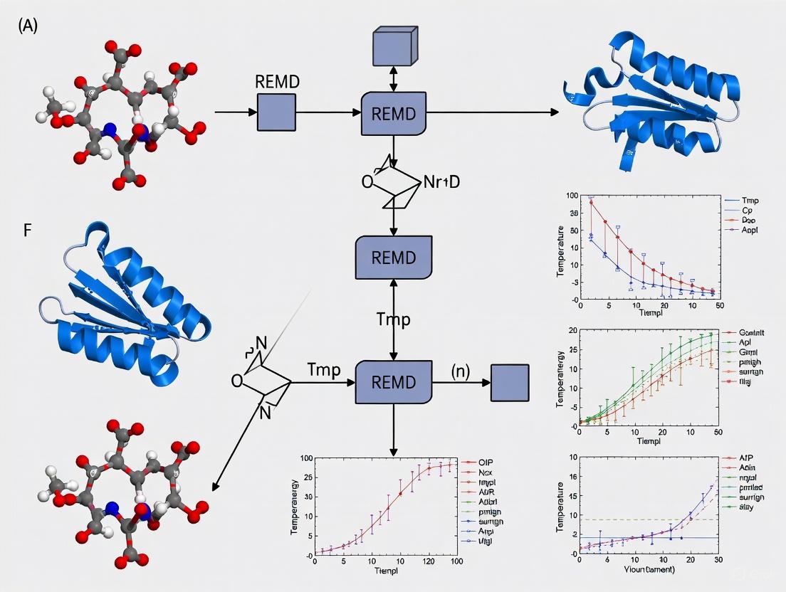
REMD Workflow and Energy Landscape Schematic

The following diagram illustrates the logical workflow of a REMD simulation and its conceptual effect on sampling the protein's energy landscape.

REMD Accelerates Conformational Sampling. The workflow (main graph) shows the cyclic process of running independent MD and attempting replica exchanges. The conceptual view illustrates how high-temperature replicas in REMD (right) can cross energy barriers that trap conventional MD simulations (left), enabling a comprehensive exploration of the energy landscape [9].

Molecular dynamics (MD) simulations are a powerful tool for studying the time evolution of biomolecular motions in atomistic resolution. However, biological molecules are characterized by a rugged free-energy landscape with many local minima separated by high-energy barriers. This makes it easy for conventional MD simulations to become trapped in local minima, unable to sample the complete conformational space within accessible simulation times—a challenge known as the "sampling problem" [11] [3]. Temperature replica exchange molecular dynamics (T-REMD), also known as parallel tempering, is an enhanced sampling technique designed to overcome this limitation [12] [11]. By simulating multiple replicas of the same system at different temperatures and periodically exchanging conformations between them, T-REMD facilitates efficient barrier crossing, enabling a more thorough exploration of the free energy landscape of biomolecules such as peptides [12] [9].

Fundamental Principles and Energetics

The Replica Exchange Concept

The T-REMD method employs a generalized ensemble approach where M non-interacting replicas of the same system are simulated simultaneously at M different temperatures [12] [11]. Each replica performs an independent molecular dynamics simulation at its assigned temperature. The core of the method lies in periodically attempting to swap the configurations of two replicas, typically neighbors in temperature space [13]. This process combines the fast sampling and frequent barrier-crossing of the highest temperature with correct Boltzmann sampling at all different temperatures [13].

Mathematical Formulation of Exchange Probability

The probability of exchanging replicas i (at temperature T(m)) and j (at temperature T(n)) is determined by the Metropolis criterion, which ensures detailed balance is maintained in the sampling process [12]. The exchange probability is given by:

[P(i \leftrightarrow j) = \min\left(1, \exp\left[ \left(\frac{1}{kB T1} - \frac{1}{kB T2}\right)(U1 - U2) \right] \right)]

where T(1) and T(2) are the reference temperatures, U(1) and U(2) are the instantaneous potential energies of the two replicas, and k(_B) is Boltzmann's constant [13]. For simulations in the isobaric-isothermal ensemble (NPT), an extension accounts for volume fluctuations:

[P(1 \leftrightarrow 2)=\min\left(1,\exp\left[ \left(\frac{1}{kB T1} - \frac{1}{kB T2}\right)(U1 - U2) + \left(\frac{P1}{kB T1} - \frac{P2}{kB T2}\right)\left(V1-V2\right) \right] \right)]

where P(1) and P(2) are reference pressures and V(1) and V(2) are instantaneous volumes [13]. After a successful exchange, the velocities of the atoms are rescaled by ((T1/T2)^{\pm0.5}) to maintain proper sampling at the new temperatures [12] [13].

Figure 1: T-REMD workflow diagram showing the replica exchange process.

Practical Implementation and Protocols

Temperature Selection and Optimization

The careful selection of temperatures is crucial for achieving adequate exchange probabilities in T-REMD simulations. The number of required replicas increases with the square root of the system size, which can make simulations of large systems in explicit solvent computationally demanding [11]. For a system with N({atoms}) atoms, the temperature spacing factor ε can be estimated as ε ≈ 1/√N({atoms}) to maintain a reasonable exchange probability [13]. The GROMACS software package provides an online REMD calculator that suggests temperature distributions based on system size and desired temperature range [11] [13].

Table 1: Temperature Selection Guidelines for T-REMD Simulations

System Type	Number of Replicas	Temperature Range (K)	Acceptance Probability Target	Key Considerations
Small peptide in explicit solvent	12-24	275-400	0.2-0.3 [11]	System size ~10-20k atoms
Medium-sized protein	24-48	278-450	>0.1	Exponential spacing often optimal
Intrinsically disordered proteins	Varies by size	278-400	0.2-0.3 [14]	Larger systems require more replicas
Using REST2 variant	Reduced (e.g., 6-12)	Same range	Similar targets	Only solute effectively "heated" [14]

Step-by-Step T-REMD Protocol for Peptide Systems

• System Preparation: Construct initial configuration of the peptide system using molecular visualization software like VMD. For peptide aggregation studies, create initial configurations with peptides separated by a reasonable distance [12].

• Parameter Setup: Prepare molecular dynamics parameters files for GROMACS, including energy minimization, equilibration, and production run settings.

• Temperature Ladder Determination: Use the GROMACS REMD calculator or similar tools to determine an optimal set of temperatures that provides acceptance probabilities of 0.2-0.3 between neighboring replicas [11] [13].

• Replica Initialization: Generate initial configurations for all replicas, which can be identical or independently equilibrated structures.

• Production Simulation: Launch parallel MD simulations with MPI-enabled GROMACS, specifying the number of replicas, temperature distribution, and exchange attempt frequency (typically every 100-1000 steps) [13].

• Exchange Protocol: GROMACS implements a symmetric exchange scheme where odd pairs (0-1, 2-3, ...) are attempted on odd steps and even pairs (1-2, 3-4, ...) on even steps to maintain detailed balance [13].

• Monitoring and Analysis: Track acceptance probabilities, replica diffusion through temperature space, and convergence of thermodynamic properties of interest.

Figure 2: T-REMD setup and execution workflow.

Performance Analysis and Optimization

Efficiency and Convergence

Studies comparing T-REMD with conventional MD demonstrate significant efficiency improvements. For a beta-heptapeptide in explicit solvent, T-REMD was approximately an order of magnitude more computationally efficient than a single 800 ns conventional MD simulation at the lowest temperature (275 K) [15]. The enhanced efficiency results from the ordering of different conformational states over temperature, facilitating better sampling of the free energy landscape [15].

Table 2: Performance Characteristics of T-REMD and Variants

Method	Computational Efficiency	Optimal Application	Limitations	Key References
Standard T-REMD	5-10x more efficient than conventional MD for small systems [15]	Peptide folding, small protein dynamics	Number of replicas scales with √N	[12] [15]
REST2	~5-6x more efficient than plain T-REMD [14]	Explicit solvent systems, membrane proteins	Altered ensemble in hot replicas	[14]
PT-WTE	~5-6x more efficient than plain T-REMD [14]	IDPs, systems with flat energy landscapes	Requires potential energy as CV	[14]
H-REMD	Varies by implementation	Free energy calculations, specific interactions	Requires parameter coupling	[13] [9]

Limitations and Advanced Variants

While powerful, T-REMD has limitations, particularly for larger systems where the number of required replicas becomes prohibitive [11] [14]. This has motivated the development of advanced variants:

• REST2 (Replica Exchange with Solute Tempering): Significantly reduces the number of replicas needed by effectively "heating" only the solute degrees of freedom while keeping the solvent at the target temperature [14].

• PT-WTE (Parallel Tempering Well-Tempered Ensemble): Combines parallel tempering with a well-tempered metadynamics bias on the potential energy, enhancing energy fluctuations and improving exchange probabilities [14].

• H-REMD (Hamiltonian Replica Exchange): Uses different Hamiltonians rather than temperatures as the replica coordinate, often implemented through scaling of specific force field parameters [13] [9].

The Scientist's Toolkit

Table 3: Essential Research Reagents and Computational Tools for T-REMD

Tool/Resource	Function/Purpose	Application Context	Availability
GROMACS [12] [13]	MD simulation package with T-REMD implementation	Primary simulation engine for REMD	Open source
VMD [12]	Molecular visualization and analysis	System setup, trajectory analysis	Free academic
MPI (Message Passing Interface)	Parallel communication library	Required for multi-replica execution	Open source
REMD Temperature Calculator [11] [13]	Optimizes temperature distribution	Protocol setup	Online tool
Amber/CHARMM/NAMD [12]	Alternative MD packages	T-REMD implementation in other frameworks	Various licenses

Application to Peptide Systems

T-REMD has proven particularly valuable in peptide research, including studies of:

• Peptide Folding and Aggregation: Revealing mechanisms of amyloid formation relevant to Alzheimer's disease, Parkinson's disease, and type II diabetes [12].

• Intrinsically Disordered Peptides: Characterizing the conformational ensembles of flexible peptides that lack stable tertiary structures [9] [14].

• Peptide-Surface Interactions: Studying adsorption behavior of peptides on inorganic surfaces for materials science applications [16].

• Cyclic Peptides: Investigating solvent-induced conformational changes and binding affinities of constrained peptide systems [11].

The method's ability to efficiently sample complex free energy landscapes makes it ideally suited for investigating peptide systems that undergo structural transitions or populate multiple conformational states, providing atomic-level insights into processes that are challenging to study experimentally.

Hamiltonian Replica Exchange Molecular Dynamics (H-REMD) represents a sophisticated advanced sampling technique that enhances conformational exploration in biomolecular simulations by systematically modifying the potential energy landscape rather than temperature. This approach addresses a fundamental limitation of conventional molecular dynamics (MD), where simulations often remain trapped in local energy minima due to high free-energy barriers. By creating multiple replicas with progressively modified Hamiltonians, H-REMD enables efficient crossing of these barriers while maintaining proper Boltzmann sampling in the reference replica. This application note details the underlying principles, methodological framework, and practical protocols for implementing H-REMD, with specific emphasis on its application to peptide systems. We provide comprehensive guidance on key parameters, efficiency optimization, and analysis techniques to facilitate successful deployment in structural biology and drug discovery research.

Molecular dynamics simulations provide atomic-level insights into biomolecular processes but face significant sampling limitations due to the rugged nature of free-energy landscapes. Conformational transitions between stable states represent rare events even on microsecond timescales, particularly for peptides and proteins with complex energy landscapes [9]. The Replica Exchange MD (REMD) methodology has emerged as one of the most powerful and widely applied advanced sampling approaches to overcome these limitations [17].

While temperature-based REMD (T-REMD) enhances sampling through thermal agitation, its computational demand grows substantially with system size, as the number of required replicas scales with the square root of the number of particles [18]. Hamiltonian REMD (H-REMD) circumvents this limitation by using the force field or Hamiltonian of the system as a replica coordinate instead of temperature [18] [9]. In this framework, different replicas simulate the system with modified potential functions while maintaining constant temperature, allowing direct manipulation of the energy barriers that impede conformational sampling.

The fundamental strength of H-REMD lies in its flexibility—researchers can selectively perturb specific energy terms or regions of the molecular system most relevant to the conformational process under investigation [9]. This targeted approach enables more efficient barrier crossing compared to generalized thermal excitation, often achieving superior sampling with fewer replicas. This application note explores the theoretical foundations, implementation protocols, and practical applications of H-REMD for peptide research, providing researchers with a comprehensive framework for leveraging this powerful methodology.

Theoretical Framework and Key Concepts

Fundamental Principles of H-REMD

H-REMD operates on the principle that multiple non-interacting copies (replicas) of a system can be simulated simultaneously using different Hamiltonians (potential energy functions). At regular intervals, exchanges between neighboring replicas are attempted according to a Metropolis criterion that preserves detailed balance [17]. For two replicas i and j with coordinates X_i and X_j and Hamiltonians H_i and H_j, the exchange probability is:

where β = 1/k_BT is the inverse temperature. This acceptance criterion ensures that the reference replica (using the unmodified Hamiltonian) samples from the correct Boltzmann distribution while benefiting from enhanced sampling in replicas with modified energy landscapes [18] [19].

Comparison of REMD Variants

Table 1: Comparison of Key REMD Sampling Approaches

Method	Replica Coordinate	Key Advantage	Primary Limitation	Ideal Application
T-REMD	Temperature	Simple implementation; universally applicable	Number of replicas grows with system size; inefficient for non-thermal barriers	Small proteins; generalized unfolding
H-REMD	Force field parameters	Targeted barrier reduction; fewer replicas required	Requires system-specific parameterization	Peptide folding; conformational transitions
BP-REMD	Biasing potential along specific coordinates	Highly efficient for predefined reaction coordinates	Limited to selected degrees of freedom	Backbone transitions; side chain rotations
aMD-HREMD	Accelerated MD boost potential	Aggressive barrier lowering; good for rare events	Complex reweighting; potential over-boosting	Large-scale conformational changes

Energy Decomposition and Hot Spot Identification

A particularly sophisticated H-REMD approach combines Hamiltonian modification with structural energy analysis to identify and target key stabilizing residues [18]. This method employs an energy decomposition approach followed by eigenvalue analysis of the resulting interaction matrix. The highest components of the eigenvector associated with the lowest eigenvalue indicate which residues ("hot spots") contribute most significantly to protein stability and folding [18]. By selectively perturbing the non-bonded interactions of these strategically important residues, the method achieves maximal destabilization of the native state with minimal modifications to the overall Hamiltonian, enabling highly efficient folding/unfolding simulations.

Protocol: H-REMD with Hot Spot Targeting

This protocol details the implementation of the energy decomposition-based H-REMD method for enhanced sampling of peptide folding/unfolding transitions, adapted from the approach successfully applied to Villin Headpiece HP35 and Protein A [18].

Preliminary Analysis and Hot Spot Identification

Objective: Identify residues crucial for structural stability that will be targeted for Hamiltonian modification.

• Equilibrium Simulation:

  • Perform a short (5-20 ns) conventional MD simulation of the folded peptide/protein in explicit solvent at the temperature of interest (typically 300 K).
  • Ensure the structure remains stable during this simulation; significant unfolding may complicate subsequent analysis.

• Energy Decomposition:

  • Extract snapshots at regular intervals (e.g., every 10-100 ps) from the equilibrium trajectory.
  • For each snapshot, compute the complete non-bonded interaction energy matrix between all residue pairs, including both electrostatic and van der Waals contributions.
  • Average these matrices over the entire trajectory to obtain a mean residue-residue interaction matrix.

• Eigenvalue Analysis:

  • Diagonalize the averaged energy matrix to obtain its eigenvalues and eigenvectors.
  • Identify the eigenvector associated with the lowest eigenvalue, which represents the most significant contributions to global stability.
  • Select residues with eigenvector components exceeding the threshold of a uniformly distributed vector (1/√N, where N is the number of residues) as "hot spots."

Table 2: Key Parameters for Hot Spot Identification

Parameter	Recommended Value	Purpose	Notes
Equilibrium MD length	5-20 ns	Generate representative folded ensemble	Must maintain structural integrity
Snapshot frequency	10-100 ps	Balance between correlation and computational cost	Adjust based on system size
Interaction cutoff	Standard MD cutoff (typically 8-10 Å)	Define residue-residue contacts	Consistent with force field
Hot spot threshold	> 1/√N	Identify significant contributors	N = number of residues

Replica Setup and Hamiltonian Modification

Objective: Create a set of replicas with progressively modified Hamiltonians targeting the identified hot spots.

• Determine Number of Replicas:

  • For the test systems (35-62 residues), 8-24 replicas provided sufficient sampling [18] [19].
  • Larger systems or more complex landscapes may require additional replicas.

• Define Hamiltonian Scaling:

  • Apply a "soft core" potential or linear scaling factor to the non-bonded interaction parameters (electrostatics and Lennard-Jones) involving the hot spot residues.
  • In replica 1 (reference), maintain the original force field parameters.
  • For replicas 2 through N, progressively weaken the interactions between hot spots and all other atoms (protein and solvent).
  • Maintain unperturbed solvent-solvent interactions to prevent artificial destabilization.

• Replica Spacing Optimization:

  • Adjust the scaling parameters to achieve approximately 20-30% exchange probabilities between neighboring replicas.
  • Perform short test simulations to verify adequate overlap in potential energy distributions between adjacent replicas.

The following workflow diagram illustrates the complete H-REMD process with hot spot targeting:

Production Simulation and Exchange Protocol

Objective: Execute the H-REMD simulation with proper exchange attempts and monitoring.

• Simulation Parameters:

  • Use a Langevin thermostat with collision frequency of 5 ps⁻¹ for temperature control [19].
  • Apply Particle Mesh Ewald for electrostatic treatment with 8.0 Å real-space cutoff.
  • Constrain bonds to hydrogen using SHAKE or LINCS to enable 2 fs time steps.

• Exchange Attempts:

  • Attempt exchanges between neighboring replicas every 1-2 ps.
  • Calculate exchange probabilities using the modified Hamiltonians according to the Metropolis criterion.
  • Implement either synchronous or asynchronous exchange protocols based on computational infrastructure.

• Convergence Monitoring:

  • Track root mean square deviation (RMSD) from native structure in the reference replica.
  • Monitor time evolution of secondary structure elements.
  • Ensure reversible folding/unfolding transitions in the reference replica.
  • Calculate round-trip times for replicas moving between extreme Hamiltonians.

Table 3: Essential Research Reagents and Computational Tools for H-REMD

Category	Specific Tool/Parameter	Function/Role	Implementation Notes
MD Engines	AMBER, GROMACS, NAMD, OpenMM	Simulation execution with H-REMD capabilities	AMBER includes specialized aMD-HREMD implementations [19]
Analysis Tools	MDAnalysis, MDTraj, PyEMMA, MSMBuilder	Trajectory analysis and Markov state modeling	MSMbuilder enables construction of kinetic models [17]
Enhanced Sampling	Accelerated MD, Metadynamics, ABF	Alternative or complementary methods	aMD applies boost potential when V(r) < E [17]
System Preparation	tLEAP, PACKMOL, CHARMM-GUI	Solvation, ionization, and system setup	Maintain ionic strength with ~100 mM NaCl [19]
Force Fields	ff12SB, ff19SB, CHARMM36, OPLS-AA	Potential energy function parameters	Choice affects conformational preferences [19]
Solvent Models	TIP3P, TIP4P, SPC/E	Explicit water representation	TIP3P is commonly used [19]

Performance Optimization and Troubleshooting

Enhancing Sampling Efficiency

• Replica Number and Spacing: For systems of ~50 residues, 8-24 replicas typically suffice [18] [19]. The key metric is maintaining 20-30% exchange rates between neighbors. If exchange rates fall below 10%, add replicas or adjust Hamiltonian differences.

• Multidimensional REMD: Combine H-REMD with temperature REMD (T-REMD) in a multidimensional approach (M-REMD) for challenging systems. This approach has demonstrated superior convergence for RNA tetranucleotides compared to single-dimensional H-REMD [19].

• Adaptive Biasing: Implement adaptive biasing of backbone and side chain dihedral angles within the H-REMD framework to specifically target the main barriers to conformational change in peptides [20].

Troubleshooting Common Issues

• Low Exchange Rates: Reduce the Hamiltonian differences between neighboring replicas or increase the number of replicas. Monitor potential energy distributions for sufficient overlap.

• Poor Convergence in Reference Replica: Extend simulation time or enhance sampling in excited states through more aggressive Hamiltonian modifications in higher replicas.

• Structural Instability: Verify that hot spot identification was performed on a stable folded trajectory. Ensure solvent-solvent interactions remain unperturbed to maintain proper solvation behavior.

• Force Field Artifacts: Be aware that strongly modified Hamiltonians may populate non-physical conformations; focus analysis on the reference replica with authentic force field parameters.

Applications and Concluding Remarks

H-REMD has proven particularly valuable for studying peptide and protein folding mechanisms, as demonstrated by its successful application to Villin Headpiece HP35 and Protein A [18]. In these cases, the method enabled reversible folding/unfolding transitions at 300 K and revealed alternative secondary structure arrangements, including beta-sheet rich structures in the primarily alpha-helical HP35 [18].

The strategic modification of potential energy landscapes through H-REMD provides researchers with a powerful tool for accelerating conformational sampling while maintaining physically meaningful ensembles. The hot spot-targeted approach further enhances efficiency by focusing computational resources on the interactions most critical to structural stability. As force fields continue to improve and computational resources expand, H-REMD methodologies are poised to make increasingly significant contributions to our understanding of peptide behavior, with direct implications for drug design and biomolecular engineering.

When implementing these protocols, researchers should carefully validate results against available experimental data and consider combining H-REMD with other advanced sampling techniques to address particularly challenging conformational transitions. The flexibility of the Hamiltonian exchange framework continues to inspire new variants and applications across diverse biomolecular systems.

Identifying Key Biomolecular Processes Ideal for REMD

Replica Exchange Molecular Dynamics (REMD) is a powerful enhanced sampling technique that overcomes the fundamental limitation of conventional molecular dynamics (MD) in simulating complex biomolecular processes. Standard MD simulations often become trapped in local energy minima, failing to sample the complete conformational space of a biological system within practical simulation timescales [12]. REMD addresses this challenge through a parallel sampling strategy that combines MD simulation with a Monte Carlo algorithm, enabling efficient exploration of complex free energy landscapes [12] [17].

The core REMD methodology involves simulating multiple non-interacting copies (replicas) of the same system simultaneously at different temperatures or with different Hamiltonians [12]. At regular intervals, exchanges between neighboring replicas are attempted based on the Metropolis criterion, which ensures detailed balance is maintained according to Boltzmann statistics [12]. This generalized ensemble approach allows high-temperature replicas to overcome significant energy barriers, while low-temperature replicas maintain proper Boltzmann sampling, resulting in dramatically enhanced conformational sampling compared to conventional MD [21].

Biomolecular Processes Ideal for REMD

Quantitative Analysis of REMD Applications

REMD has demonstrated particular effectiveness for specific classes of biomolecular processes characterized by high energy barriers and complex free energy landscapes. The table below summarizes key biomolecular processes where REMD provides significant advantages over conventional MD simulations.

Table 1: Key Biomolecular Processes Ideal for REMD Simulation

Biomolecular Process	Specific Applications	Sampling Challenge	REMD Benefit	Representative Systems
Protein & Peptide Aggregation	Amyloid formation, oligomerization	Multiple intermediate states, kinetic traps	Overcomes high energy barriers between aggregation states	hIAPP(11-25), Aβ peptides [12] [21]
Protein Folding	Mini-protein folding, secondary structure formation	Rugged free energy landscape, multiple pathways	Enhances sampling of folded/unfolded states	Trp-cage, β-hairpins, α-helix formation [22] [21]
Membrane-Protein Interactions	Fusion peptide opening, membrane association	Slow lipid reorganization, insertion kinetics	Samples insertion depths and membrane-bound conformations	SARS-CoV-2 fusion peptide, membrane proteins [21] [23]
Protein-Ligand Binding	Drug discovery, binding affinity calculations	Rare binding/unbinding events, pose transitions	Improves binding pose sampling and affinity predictions	Small molecule inhibitors, therapeutic design [21]
Structure Prediction	Cyclic peptides, protein model refinement	Conformational diversity, native state identification	Efficiently explores conformational space	Cyclic peptides, small proteins [22]

Detailed Analysis of Ideal Application Areas

Protein Aggregation and Amyloid Formation: REMD is particularly valuable for studying protein aggregation phenomena associated with neurodegenerative diseases and type II diabetes [12]. The early stages of aggregation involve fast processes and transient oligomers that are challenging to characterize experimentally. The REMD method efficiently samples these aggregation pathways, revealing intermediate states and free energy landscapes critical for understanding disease mechanisms and developing inhibitors [12].

Protein Folding Studies: For protein folding applications, REMD has proven capable of predicting structures of peptides and small proteins with accuracy comparable to experimental methods [22]. Studies on systems like the Trp-cage mini-protein demonstrate that REMD can quickly form secondary structural elements, though detailed free-energy surface convergence may require extended simulation times [21]. The mean time for replicas to sample both folded and unfolded basins for Trp-cage is approximately 20 ns, suggesting equilibrium calculations should extend well beyond this duration for proper convergence [21].

Membrane-Associated Processes: REMD simulations provide unique insights into membrane-related processes such as fusion peptide opening in viral spike proteins. For SARS-CoV-2, REMD has helped elucidate how proteolytic cleavage state affects fusion peptide flexibility, revealing opening dynamics on the submicrosecond timescale [23]. This understanding facilitates the development of inhibition strategies that target these conformational changes.

REMD Methodologies and Protocols

Fundamental REMD Algorithm

The theoretical foundation of REMD involves creating a generalized ensemble where M non-interacting replicas of the system are simulated at M different temperatures [12]. The state of this generalized ensemble is described by:

Figure 1: REMD Workflow and Exchange Mechanism

The mathematical implementation follows these key equations. The Hamiltonian of the system is defined as H(q,p) = K(p) + V(q), where K(p) represents kinetic energy and V(q) represents potential energy [12]. In the canonical ensemble, the probability of finding the system in state x≡(q,p) at temperature T is ρB(x,T) = exp[-βH(q,p)], where β = 1/kBT [12].

For replica exchange between replicas i (at temperature Tm) and j (at temperature Tn), the transition probability follows the Metropolis criterion:

w(X→X′) ≡ w(xm[i]|xn[j]) = min(1, exp(-Δ))

where Δ = (βn - βm)(V(q[i]) - V(q[j])) [12]

This formulation ensures detailed balance is maintained while enabling efficient sampling across temperatures.

Practical Implementation Protocol

Case Study: hIAPP(11-25) Dimer Aggregation

Figure 2: REMD Experimental Workflow for Peptide Aggregation Study

Step-by-Step Protocol:

• Initial System Preparation: Construct the initial configuration of the biomolecular system. For hIAPP(11-25) dimer studies, this involves creating two peptides with amino acid sequence RLANFLVHSSNNFGA, capped with an acetyl group at the N-terminus and NH₂ group at the C-terminus [12]. Multiple initial configurations may be necessary for complex systems.

• Solvation and Equilibration: Solvate the system in an appropriate water model (e.g., TIP3P) and add ions to achieve physiological concentration. Perform energy minimization followed by conventional NVT and NPT equilibration to stabilize temperature and pressure [12].

• Temperature Selection and Replica Setup: Conduct short pilot simulations at different temperatures to determine optimal temperature distribution. The temperature spacing should yield approximately 15-20% exchange probability between neighboring replicas [12]. For the hIAPP(11-25) dimer, typical temperature ranges span from 270K to 600K distributed across 24-64 replicas, depending on system size and computational resources.

• REMD Production Simulation: Launch parallel REMD simulations using MPI-enabled GROMACS. Key parameters include:

  • Exchange attempt frequency: Every 1-2 ps
  • Integration time step: 2 fs (or 4 fs with hydrogen mass repartitioning)
  • Thermostat: Langevin or Nosé-Hoover
  • Barostat: Parrinello-Rahman (for NPT ensemble)
  • Simulation duration: 50-200 ns per replica for convergence [12] [21]

• Trajectory Analysis and Validation: Process replica trajectories to construct continuous pathways at reference temperatures. Analyze using:

  • Root mean square deviation (RMSD) for structural stability
  • Radius of gyration for compactness
  • Secondary structure analysis (DSSP)
  • Free energy landscape projection using principal component analysis
  • Markov State Models for kinetic information [12] [17]

The Scientist's Toolkit

Table 2: Essential Research Reagents and Computational Tools for REMD

Category	Item	Specification	Function/Purpose
Software Packages	GROMACS-4.5.3+	With MPI support	Primary MD engine for REMD simulations [12]
	AMBER, CHARMM, NAMD	Latest stable versions	Alternative MD packages supporting REMD [12]
	VMD	Version 1.9.3+	Molecular visualization and trajectory analysis [12]
Force Fields	CHARMM36	All-atom with CMAP	Protein and lipid force fields [23]
	AMBER94	All-atom	Protein force field for folding studies [21]
	TIP3P, TIP4P	Water models	Solvation environment [21]
Computational Resources	HPC Cluster	Intel Xeon X5650+ CPUs, Infiniband	Parallel computing infrastructure [12]
	MPI Library	MPICH, OpenMPI	Message passing interface for parallelization [12]
Analysis Tools	PyEMMA	Version 2.0+	Markov State Model construction [17]
	MSMBuilder	Version 3.0+	Kinetic model building from trajectories [17]
System Components	Peptide Models	Acetyl/NH₂ capping	Proper terminal charge representation [12]
	Ion Concentrations	0.15M NaCl	Physiological ionic strength [12]

Practical Implementation Notes

Temperature Optimization: Efficient temperature selection is critical for REMD success. For a system with M replicas, temperatures should be spaced to maintain consistent exchange rates. The optimal temperature distribution can be determined through short pilot simulations (3-5 ns) measuring potential energy distributions across a broad temperature range (270-600K) [12]. For the hIAPP(11-25) dimer system, this typically results in approximately 24-32 replicas to maintain 15% exchange probability [12].

Convergence Assessment: REMD simulations require careful monitoring to ensure proper convergence. Key indicators include:

• Replica diffusion through temperature space
• Stationarity of potential energy and structural metrics
• Convergence of free energy differences between states For the Trp-cage mini-protein, studies indicate that mean folding/unfolding transition times of ~20 ns require simulation lengths extending many times this duration for proper equilibrium [21].

Enhanced Variants: Several REMD extensions have been developed for specialized applications:

• Replica Exchange Umbrella Sampling (REUS): Combines REMD with umbrella sampling [17]
• Hamiltonian REMD: Employs different Hamiltonians rather than temperatures [17]
• Temperature and Volume REMD: Samples different pressure states [21]
• Replica Exchange Constant-pH: Incorporates pH as an exchange dimension [17]

Advanced Applications and Future Directions

REMD continues to evolve with emerging methodologies that expand its applicability to increasingly complex biological systems. Recent advances include integration with hydrogen mass repartitioning (HMR) to enable 4 fs time steps, effectively doubling simulation efficiency without significant loss of accuracy [17]. This approach increases hydrogen atom mass to approximately 3 amu while decreasing bonded heavy atom mass accordingly, allowing larger integration steps while maintaining stable simulations [17].

The method has also been successfully integrated with Markov State Models (MSMs) to create comprehensive kinetic models of biomolecular processes [17] [23]. This hybrid approach uses many short REMD simulations to efficiently sample conformational space, then constructs MSMs to identify metastable states and transition pathways [17]. For the SARS-CoV-2 spike protein, this protocol has revealed fusion peptide opening dynamics and identified potential small-molecule binding sites to inhibit conformational changes required for host-cell infection [23].

Future developments focus on improving scalability for larger systems and enhancing integration with experimental data. Challenges remain in applying REMD to membrane-protein systems and large macromolecular complexes, where the number of required replicas grows substantially [21]. Emerging solutions include hybrid Hamiltonian/temperature exchanges and targeted sampling methods that focus enhancement on specific functional regions, promising to extend REMD's utility for drug discovery and biomolecular engineering.

Setting Up Your REMD Simulation: A Step-by-Step Protocol for Peptides

Replica Exchange Molecular Dynamics (REMD) has become an indispensable enhanced sampling technique for studying complex biomolecular processes, such as peptide folding and aggregation, that occur on timescales beyond the reach of conventional molecular dynamics (MD). The fundamental challenge in MD simulations is that systems often become trapped in local energy minima, failing to sample the full conformational landscape within practical simulation timescales [3]. REMD addresses this limitation by running multiple parallel simulations (replicas) of the same system under different conditions and periodically attempting exchanges between them according to a Metropolis criterion, thereby accelerating barrier crossing while maintaining proper thermodynamic sampling [12].

The two principal variants of this method, Temperature REMD (T-REMD) and Hamiltonian REMD (H-REMD), offer distinct mechanistic approaches and practical considerations for enhancing sampling. T-REMD, the original and more widely implemented form, differs from H-REMD in the parameter used to distinguish replicas: temperature versus the system's Hamiltonian. This fundamental distinction leads to significant differences in their applications, efficiency, and implementation requirements, making the choice between them critical for researchers, particularly those investigating peptide systems for drug development [3] [24].

This application note provides a structured comparison of T-REMD and H-REMD methodologies, detailing their theoretical foundations, practical implementation protocols, and optimal application domains to guide researchers in selecting the most appropriate approach for their specific peptide systems.

Theoretical Foundations and Comparative Analysis

Temperature Replica Exchange MD (T-REMD)

In T-REMD, multiple non-interacting copies (replicas) of the system are simulated simultaneously at different temperatures. The key concept is that higher-temperature replicas can overcome significant energy barriers more easily, exploring a broader conformational space. Periodically, exchanges between neighboring temperatures are attempted with a probability given by:

[P(1 \leftrightarrow 2)=\min\left(1,\exp\left[ \left(\frac{1}{kB T1} - \frac{1}{kB T2}\right)(U1 - U2) \right] \right)]

where (T1) and (T2) are the reference temperatures and (U1) and (U2) are the instantaneous potential energies of the two replicas, respectively [24]. After a successful exchange, velocities are scaled by ((T1/T2)^{\pm0.5}) to maintain proper ensemble distributions.

The primary advantage of T-REMD is its conceptual and implementation simplicity, as it requires modification only of the simulation temperature. However, its computational cost scales with system size because the number of replicas required to maintain adequate exchange probabilities grows approximately with the square root of the number of degrees of freedom [24]. For large biomolecular systems such as solvated peptides, this can require dozens or even hundreds of replicas, representing a significant computational investment [19] [25].

Hamiltonian Replica Exchange MD (H-REMD)

H-REMD, also known as Parallel Tempering with Expanded Ensembles, employs a different strategy. Instead of varying temperature, replicas simulate the system with different Hamiltonians, typically achieved by altering the potential energy function through a coupling parameter λ [24]. The exchange probability between two replicas with different Hamiltonians is:

[P(1 \leftrightarrow 2)=\min\left(1,\exp\left[ \frac{1}{kB T} (U1(x1) - U1(x2) + U2(x2) - U2(x_1)) \right]\right)]

where (U1) and (U2) represent the different potential energy functions [24].

A key advantage of H-REMD is its flexibility in selecting which degrees of freedom to bias. Common approaches include scaling dihedral force constants (DFC) to enhance torsional sampling [19] or applying a boosting potential as in accelerated MD (aMD) [19] [25]. By focusing the biasing potential on specific, hard-to-sample degrees of freedom, H-REMD can provide more efficient sampling for particular conformational transitions while requiring fewer replicas than T-REMD for the same system size [19] [25].

Table 1: Quantitative Comparison of T-REMD and H-REMD Approaches

Feature	T-REMD	H-REMD
Replica Difference	Temperature	Hamiltonian (Potential Energy Function)
Exchange Probability Formula	(\min\left(1,\exp\left[ \left(\frac{1}{kB T1} - \frac{1}{kB T2}\right)(U1 - U2) \right] \right)) [24]	(\min\left(1,\exp\left[ \frac{1}{kB T} (U1(x1) - U1(x2) + U2(x2) - U2(x_1)) \right]\right)) [24]
Replica Scaling with System Size	Scales with (\sqrt{N_{atoms}}) [24]	More system-dependent; typically fewer replicas required [19]
Computational Cost	High for large systems due to many replicas	Lower replica count but potentially more complex energy calculations
Optimal Application	General enhanced sampling; systems with temperature-dependent barriers [3]	Targeting specific conformational changes (e.g., torsional transitions, ligand binding) [19]
Implementation Complexity	Lower	Higher
Reweighting Complexity	Straightforward	More challenging

Multidimensional REMD (M-REMD)

For particularly challenging sampling problems, combining both temperature and Hamiltonian dimensions in Multidimensional REMD (M-REMD) can provide superior sampling efficiency. The acceptance probability for this combined approach becomes:

[P(1 \leftrightarrow 2)=\min\left(1,\exp\left[ \frac{U1(x1) - U1(x2)}{kB T1} + \frac{U2(x2) - U2(x1)}{kB T2} \right] \right)]

where replicas differ in both temperature and Hamiltonian [24]. Studies on RNA tetranucleotides have demonstrated that M-REMD can sample rare conformations more efficiently than either method alone, though at significantly increased computational cost [19].

Decision Framework and Selection Guidelines

The choice between T-REMD and H-REMD depends on multiple factors, including system characteristics, computational resources, and scientific objectives. The following decision framework provides guidance for selecting the appropriate method:

Choose T-REMD when:

• Studying small to medium-sized peptides (typically < 50 amino acids)
• A general, unbiased exploration of conformational space is desired
• Computational resources allow for sufficient replicas to maintain exchange probabilities > 20%
• The system lacks obvious reaction coordinates for biasing

Choose H-REMD when:

• Investigating specific conformational transitions with known slow degrees of freedom (e.g., proline isomerization, ring puckering)
• Working with larger systems where T-REMD would require prohibitive numbers of replicas
• Targeting particular states or intermediates in peptide folding pathways
• Prior knowledge suggests specific torsion angles or distances as good reaction coordinates

Consider M-REMD when:

• Studying highly complex systems with multiple slow degrees of freedom
• Both global unfolding and localized conformational changes are relevant
• Maximum sampling efficiency is critical despite higher computational cost

The following diagram illustrates the logical decision process for selecting the appropriate REMD method:

Implementation Protocols

T-REMD Implementation for Peptide Systems

Step 1: System Preparation

• Construct initial peptide coordinates using molecular modeling software (e.g., CHARMM-GUI, LEaP)
• Solvate in an appropriate water model (TIP3P, TIP4P) with sufficient padding (≥10 Å)
• Add ions to neutralize system and achieve physiological concentration (e.g., 150 mM NaCl)
• Energy minimize using steepest descent/conjugate gradient until convergence (<1000 kJ/mol/nm)

Step 2: Temperature Distribution Optimization

• Calculate number of replicas using (N \approx 1 + 2.2\sqrt{N_{atoms}}) as initial estimate
• Use REMD calculator tools (available in GROMACS, AMBER) to optimize temperature distribution
• Target exchange probabilities of 20-40% between adjacent replicas
• For a 50-residue solvated peptide, typically 24-48 replicas are required

Step 3: Equilibration Protocol

• Perform gradual heating from 0 K to target temperatures over 100-200 ps
• Apply position restraints on peptide heavy atoms during initial equilibration
• Conduct short (1-2 ns) canonical MD at each temperature before initiating exchanges

Step 4: Production Simulation

• Set exchange attempt frequency to 1-2 ps(^{-1}) (every 500-1000 steps for 2 fs timestep)
• Run simulations for sufficient time to observe multiple round trips between temperature extremes
• For peptide folding studies, typical simulation times range from 100-500 ns/replica

Step 5: Analysis and Validation

• Monitor round-trip times between lowest and highest temperatures
• Calculate potential energy and radius of gyration distributions across replicas
• Validate against available experimental data (NMR, CD spectroscopy)

H-REMD Implementation with Accelerated MD

Step 1: Hamiltonian Parameterization

• Select appropriate biasing method (aMD, GaMD, DFC scaling)
• For aMD on torsions: calculate average dihedral energy from short conventional MD
• Set boost potential parameters: (E{threshold} = V{avg} + 4-5 \times V{std}), ( \alpha = 0.2 \times V{std} )
• Create λ schedule for Hamiltonian interpolation (typically 8-24 replicas)

Step 2: System Setup

• Prepare identical system coordinates across all replicas
• Modify simulation parameters to implement different Hamiltonians for each replica
• For AMBER: Modify aMD boost parameters in mdin files
• For GROMACS: Use free-energy functionality with λ-dynamics

Step 3: Enhanced Equilibration

• Run conventional MD to establish baseline distributions
• Gradually introduce biasing potential across replicas
• Ensure proper equilibration at each Hamiltonian state

Step 4: Production Run with Exchanges

• Attempt exchanges every 1-2 ps
• Use Gibbs sampling or neighbor-only exchange schemes
• For a 24-residue peptide, simulation times of 50-200 ns/replica are typical

Step 5: Analysis and Reweighting

• Use MBAR or WHAM for proper statistical reweighting [19]
• Calculate conformational populations and free energy surfaces
• Compare biased and unbiased ensembles for consistency

Table 2: Key Research Reagent Solutions for REMD Simulations

Resource Type	Specific Examples	Function/Purpose
MD Software Packages	GROMACS [12] [24], AMBER [19] [26], NAMD [3], CHARMM [12]	Core simulation engines with REMD implementations
Force Fields	AMBER FF99SB [26], FF12SB [19], FF14SB [26], CHARMM36m	Parameter sets defining molecular interactions
Solvent Models	TIP3P [19] [26], TIP4P, GBOBC (implicit) [26]	Water representation for solvated systems
Enhanced Sampling Modules	aMD [19], GaMD [27], Metadynamics [3] [28]	Hamiltonian modification methods for H-REMD
Analysis Tools	MDTraj, PyEMMA, MDAnalysis, CPPTRAJ, VMD [12]	Trajectory analysis and visualization
Reweighting Methods	MBAR [25], WHAM, Bennet Acceptance Ratio	Recovering unbiased statistics from biased ensembles

Application Case Studies

T-REMD for Amyloid-β Peptide Aggregation

In studies of amyloid-β peptides involved in Alzheimer's disease pathogenesis, T-REMD has been extensively employed to explore early aggregation events. Simulations of Aβ fragments (e.g., Aβ16-22) using 24-48 replicas across 280-400 K have revealed nucleation pathways and polymorphic fibril structures. These simulations successfully identified β-sheet formation intermediates and salt bridge patterns that stabilize oligomeric structures, providing molecular insights into amyloid formation mechanisms that align with solid-state NMR constraints [29].

H-REMD for Proline Isomerization in Disordered Peptides

The application of H-REMD with accelerated MD specifically targeting torsional angles proved highly effective for studying proline isomerization in the intrinsically disordered protein ArkA. Unlike conventional MD or T-REMD, this approach successfully captured cis-trans isomerization events for all five prolines in the sequence, revealing a more compact ensemble with reduced polyproline II helix content that better matched experimental circular dichroism data. This demonstrated H-REMD's superior efficiency for sampling specific conformational transitions with high energy barriers [27].

M-REMD for RNA Tetranucleotide Conformational Sampling

A comparative study on the RNA tetranucleotide r(GACC) demonstrated the superior sampling efficiency of M-REMD over single-dimension REMD approaches. While H-REMD with 8 replicas using aMD failed to sample certain rare conformations, M-REMD with 192 replicas combining temperature and Hamiltonian dimensions achieved significantly better convergence and identified conformational states inaccessible to either method alone. This came at substantial computational cost but provided a more complete description of the conformational landscape [19].

Advanced Integration and Future Directions

The field of enhanced sampling continues to evolve with emerging methodologies that combine REMD with other computational approaches:

Integration with AI Methods: Recent advances incorporate deep learning, particularly Denoising Diffusion Probabilistic Models (DDPMs), with REST2 (a variant of H-REMD) to improve free energy landscape reconstruction. These hybrid approaches leverage generative models to enhance sampling of high-barrier regions while requiring fewer replicas than conventional T-REMD [25] [27].

Collective Variable Biasing Combinations: Methods like metadynamics and umbrella sampling are increasingly combined with REMD frameworks to focus sampling along specific reaction coordinates while maintaining broader conformational exploration [28].

Advanced Solvation Models: The use of implicit solvent models like Generalized Born in REMD simulations significantly reduces computational cost by eliminating explicit solvent degrees of freedom. While this introduces approximations, it enables much longer timescale sampling, with demonstrated effectiveness for protein folding and peptide aggregation studies [26].

These developments point toward increasingly sophisticated multi-method approaches that leverage the respective strengths of different enhanced sampling techniques to tackle the most challenging problems in peptide conformational dynamics and drug discovery.

Molecular dynamics (MD) simulations provide powerful insights into peptide structure and dynamics at an atomic level. However, conventional MD simulations often struggle to adequately sample the complete conformational space of peptide systems within practical timeframes, as they can become trapped in local energy minima [12] [30]. This limitation is particularly problematic for studying complex processes like peptide aggregation and folding, which involve high energy barriers and multiple metastable states [12] [22]. Enhanced sampling methods effectively address this challenge by accelerating the exploration of conformational space.

Replica Exchange Molecular Dynamics (REMD) has emerged as a particularly effective enhanced sampling technique for peptide research [12] [31]. By running multiple parallel simulations (replicas) at different temperatures and periodically attempting exchanges between them based on the Metropolis criterion, REMD enables systems to overcome energy barriers more efficiently than conventional MD [12]. This protocol provides a comprehensive practical workflow for implementing REMD simulations, from initial structure preparation through to production runs and analysis, specifically tailored to peptide systems relevant to drug development research.

Theoretical Foundation of Replica Exchange MD

The REMD algorithm creates a generalized ensemble where M non-interacting copies (replicas) of the system are simulated simultaneously at different temperatures [12]. Each replica i evolves independently at its assigned temperature T_m according to standard molecular dynamics. Periodically, exchanges between neighboring replicas are attempted with acceptance probability given by:

w(X→X′) = min(1, exp(-Δ))

where Δ = (βn - βm)(V(q[i]) - V(q[j])), with β = 1/kBT, kB being Boltzmann's constant, T the absolute temperature, and V(q) the potential energy [12]. This approach satisfies the detailed balance condition and ensures proper sampling of the canonical ensemble. The fundamental advantage of this method is that conformations sampled at higher temperatures can overcome energy barriers and subsequently propagate to lower temperatures, leading to more thorough conformational sampling compared to conventional MD [12].

A Practical REMD Workflow for Peptide Systems

The following diagram illustrates the complete REMD workflow from initial structure preparation through to production simulation and analysis:

Initial System Preparation

3.2.1 Constructing the Initial Peptide Structure

The first step involves constructing a starting configuration of your peptide system. For the example of studying the dimerization of the hIAPP(11-25) fragment (sequence: RLANFLVHSSNNFGA), initial structures can be built using molecular visualization software like VMD [12]. The peptide should be properly capped with an acetyl group (CH₃CO-) at the N-terminus and a NH₂ group at the C-terminus to mimic experimental conditions [12]. When studying aggregation, initial configurations may place peptides in various orientations to avoid bias.

3.2.2 Solvation and Energy Minimization

After constructing the peptide structure, the system must be solvated in an appropriate water model and ion concentration. Following solvation, energy minimization is critical to remove any steric clashes and bad contacts introduced during system setup. This is typically performed using steepest descent or conjugate gradient algorithms until the maximum force falls below a specified threshold (e.g., 1000 kJ/mol/nm) [12].

3.2.3 System Equilibration

Proper equilibration prepares the minimized system for production REMD simulations:

• NVT Equilibration: This phase stabilizes the temperature of the system using a thermostat (e.g., Berendsen or Nosé-Hoover) for a typical duration of 100-500 ps.
• NPT Equilibration: This phase adjusts the density of the system using a barostat (e.g., Parrinello-Rahman) to achieve the desired pressure, typically for 100-500 ps.

Equilibration should be performed for each replica at its respective temperature to ensure proper initialization of the REMD simulation [12].

REMD-Specific Setup

3.3.1 Temperature Distribution Selection

Choosing an appropriate temperature distribution across replicas is crucial for achieving high exchange probabilities in REMD simulations. The temperature range should span from the temperature of interest (often 300 K) to the highest temperature where the peptide remains stable. The number of replicas required depends on system size and temperature range, and can be estimated using the formula:

Nreplicas ≈ 1 + 3.3 × log₁₀(Natoms) [12]

Table 1: Example Temperature Distributions for Different System Sizes

System Size (Atoms)	Temperature Range (K)	Number of Replicas	Exchange Probability Target
5,000-10,000	300-500	24-32	15-25%
10,000-20,000	300-450	32-48	15-25%
20,000-50,000	300-400	48-64	15-25%

3.3.2 Parameter Configuration for REMD

Key parameters must be specified in the MD configuration file for REMD simulations:

• Exchange Attempt Frequency: Typically every 100-1000 steps (2-10 ps)
• Neighbor Search Cutoff: Usually 1-1.2 nm
• Thermostat: Nosé-Hoover or velocity rescale with appropriate time constants
• Barostat (for NPT-REMD): Parrinello-Rahman with time constant of 2-5 ps

Production REMD Run

Execution of REMD simulations requires a high-performance computing (HPC) cluster with MPI support. For GROMACS, the typical command is:

mpirun -np N_replicas mdrun_mpi -s topol.tpr -multi M -replex N_exchange_attempts

where Nreplicas matches the number of temperatures, and Nexchange_attempts defines how frequently exchange is attempted [12]. Monitoring during runtime should include checking exchange probabilities, temperature distributions, and potential energy fluctuations to ensure proper sampling.

Post-Simulation Analysis

3.5.1 Trajectory Analysis

After completing REMD simulations, analysis focuses on reconstructing continuous trajectories and calculating thermodynamic and structural properties:

• Replica Trajectory Processing: Use tools like gromacs analysis utilities to process trajectories from different replicas and temperatures
• Conformational Clustering: Identify dominant conformational states using algorithms like GROMOS or k-means
• Secondary Structure Analysis: Calculate temporal evolution of secondary structure elements using DSSP or STRIDE
• Contact Maps and Distance Analysis: Identify persistent intermolecular contacts in peptide aggregates

3.5.2 Free Energy Landscape Calculation

REMD enables construction of free energy landscapes along relevant collective variables (CVs) such as radius of gyration, root-mean-square deviation (RMSD), or number of native contacts. The free energy is calculated as:

G(ξ) = -k_BT ln P(ξ)

where P(ξ) is the probability distribution along collective variable ξ [12]. These landscapes reveal metastable states, transition states, and energy barriers governing peptide conformational dynamics and aggregation.

Research Reagent Solutions

Table 2: Essential Research Reagents and Computational Tools for REMD Simulations

Item Name	Function/Application	Example Options	Implementation Notes
MD Software	Engine for running simulations	GROMACS [12], AMBER [12], NAMD [30], CHARMM [12]	GROMACS recommended for REMD due to excellent parallelization
Force Field	Defines molecular interactions	GROMOS 54A7/54B7 [32] [33], AMBER99SB [30]	GROMOS 54A7 provides corrected helical propensities [32]
Visualization Tool	Structure building and analysis	VMD (Visual Molecular Dynamics) [12]	Essential for initial structure preparation and trajectory visualization
HPC Cluster	Computational resources	MPI-enabled clusters [12]	Typically 2 cores per replica for optimal performance [12]
Solvent Model	Hydration environment	SPC, TIP3P, TIP4P	Choice affects peptide solvation and dynamics

Case Study: hIAPP(11-25) Dimerization

To illustrate this workflow, we consider a case study of the dimerization of the 11-25 fragment of human islet amyloid polypeptide (hIAPP) [12]. This system is relevant to type II diabetes research and demonstrates the application of REMD to peptide aggregation.

Following the workflow outlined above, researchers constructed initial configurations of hIAPP(11-25) monomers placed in random orientations using VMD [12]. After solvation, energy minimization, and equilibration, they performed REMD simulations with 32 replicas spanning 300-500 K. Exchange attempts were made every 2 ps, maintaining an exchange probability of 18-22%. Production runs of 100 ns per replica enabled comprehensive sampling of dimer conformations.

Analysis revealed multiple dimeric states with varying β-sheet content, providing molecular insights into early aggregation events linked to amyloid formation. The free energy landscape constructed along RMSD and radius of gyration coordinates identified stable dimer configurations and transition pathways between them [12]. This case study demonstrates how the REMD workflow can yield atomistic insights into peptide aggregation mechanisms relevant to disease pathology.

Troubleshooting Common Issues

Successful REMD implementation requires addressing several common challenges:

• Low Exchange Rates: If exchange probabilities fall below 10%, adjust temperature distribution by adding more replicas or optimizing temperature spacing
• Replica Degradation: Ensure sufficient equilibration at each temperature before production runs
• System Size Limitations: For large systems, consider Hamiltonian REMD or solute-tempering variants to reduce replica count
• Analysis Complexity: Use automated scripts to process multiple replica trajectories and compute ensemble averages

The provided workflow establishes a robust foundation for implementing REMD simulations of peptide systems, enabling researchers to overcome sampling limitations and obtain statistically meaningful conformational ensembles for drug development applications.

Replica Exchange Molecular Dynamics (REMD) has emerged as a pivotal method for enhancing the sampling of conformational space in biomolecular simulations, particularly for complex processes like peptide aggregation and protein folding. The efficacy of REMD simulations, however, is profoundly dependent on the careful selection of critical parameters: replica count, temperature spacing, and Hamiltonian design. improper parameter choices can lead to poor replica exchange rates, inefficient sampling, and ultimately, non-convergent simulations. This application note provides detailed protocols and evidence-based guidelines for optimizing these parameters within the GROMACS simulation framework, aiming to equip researchers with the tools to design robust and efficient REMD studies for peptide research and drug development.

Theoretical Foundation of Replica Exchange

Fundamental Principles

REMD operates by running multiple non-interacting replicas of a system in parallel at different thermodynamic states (e.g., different temperatures or Hamiltonians). At regular intervals, exchanges between neighboring replicas are attempted based on a Metropolis criterion that preserves detailed balance. For temperature-based REMD (T-REMD), the exchange probability between two replicas at temperatures ( Ti ) and ( Tj ), with potential energies ( Ui ) and ( Uj ), is given by:

[P(i \leftrightarrow j) = \min\left(1,\exp\left[ \left(\frac{1}{kB Ti} - \frac{1}{kB Tj}\right)(Ui - Uj) \right] \right)]

where ( k_B ) is Boltzmann's constant [34]. This equation highlights that the exchange probability depends on both the temperature difference and the potential energy difference between the two replicas.

Generalized Ensemble and Sampling Enhancement

The power of REMD lies in its creation of a generalized ensemble, where the combined system of all replicas can overcome high free-energy barriers that would trap conventional MD simulations. High-temperature replicas can explore extended conformations and cross barriers, while low-temperature replicas provide accurate Boltzmann sampling. The random walk in temperature space allows conformations to diffuse throughout the temperature range, facilitating thorough exploration of the conformational landscape [12] [35]. The workflow below illustrates this core principle.

Determining Replica Count and Temperature Spacing

Analytical Foundations for Parameter Selection

The number of replicas required and the temperature spacing between them are interdependent and critically depend on the system size. The goal is to achieve a sufficient exchange acceptance rate (often recommended to be between 10% and 30%) between all neighboring replicas to ensure a random walk through temperature space. The energy difference between replicas can be approximated as:

[U1 - U2 = N{df} \frac{c}{2} kB (T1 - T2)]

where ( N_{df} ) is the total number of degrees of freedom, and ( c ) is a system-dependent constant (approximately 1 for harmonic potentials and around 2 for protein/water systems) [34]. This relationship directly links system size to the expected energy variance.

For a temperature spacing of ( T2 = (1+\epsilon)T1 ), the exchange probability can be approximated as:

[P(1 \leftrightarrow 2) \approx \exp\left(-\epsilon^2 \frac{c}{2} N_{df} \right)]

To maintain a constant acceptance probability, the relative temperature spacing ( \epsilon ) should scale as ( 1/\sqrt{N{df}} ). With all bonds constrained, ( N{df} \approx 2 N{atoms} ), leading to the practical guideline: ( \epsilon \approx 1/\sqrt{N{atoms}} ) for systems with ( c = 2 ) [34].

Practical Temperature Selection and Optimization

For a typical peptide-water system with constraints on all bonds, the number of degrees of freedom is approximately twice the number of atoms. The GROMACS documentation suggests using a REMD calculator that incorporates the temperature range and number of atoms to propose an appropriate set of temperatures [34]. It is important to note that when using pressure coupling, the density change at higher temperatures can affect potential energies and should be considered during parameter optimization [34].

The table below provides concrete examples of how replica counts and temperatures scale with system size for a target acceptance rate of ~20%.

Table 1: Replica Configuration Examples for Different System Sizes

System Description	Approximate Number of Atoms	Recommended Number of Replicas	Temperature Spacing (K)	Temperature Range (K)
Small peptide (e.g., 10 residues in water)	5,000	8-12	5-10	300 - 400
Medium peptide (e.g., 25 residues in water)	15,000	16-24	3-7	300 - 450
Large peptide/protein (e.g., 50 residues in water)	40,000	24-32	2-4	300 - 500

Exchange Schemes and Attempt Frequencies

GROMACS implements a scheme where exchange attempts are alternated between odd and even pairs of replicas to maintain detailed balance. For instance, with four replicas (0, 1, 2, 3), pairs (0-1) and (2-3) are attempted on odd-numbered attempts (e.g., 1000, 3000 steps), while pair (1-2) is attempted on even-numbered attempts (e.g., 2000, 4000 steps) [34]. This ensures that the exchange process is unbiased. The exchange frequency should be chosen to allow the system to decorrelate between attempts, typically every 100-1000 MD steps, balancing communication overhead with sampling efficiency.

Hamiltonian Replica Exchange Molecular Dynamics (H-REMD)

Principles and Advantages

Hamiltonian REMD (H-REMD) addresses a key limitation of T-REMD: the rapidly increasing number of required replicas with system size. In H-REMD, replicas are simulated at the same temperature but with different Hamiltonians (force fields), often corresponding to different points along a λ pathway in free energy calculations [34] [18]. The exchange probability for H-REMD is:

[P(1 \leftrightarrow 2)=\min\left(1,\exp\left[ \frac{1}{kB T} (U1(x1) - U1(x2) + U2(x2) - U2(x_1)) \right]\right)]

where ( U1 ) and ( U2 ) represent the potential energies of the two different Hamiltonians [34]. By focusing the modifications on a specific part of the system, H-REMD can achieve efficient sampling with significantly fewer replicas than T-REMD [18].

Advanced H-REMD Protocols: "Hot-Spot" Identification

A sophisticated H-REMD protocol leverages the energy decomposition method to identify key residues—folding "hot spots"—that are crucial for structural stability. The protocol involves:

• Energy Network Analysis: Running a short, conventional MD simulation of the folded protein and decomposing the non-bonded interaction energy matrix between residues.
• Eigenvalue Decomposition: Diagonalizing this energy matrix and analyzing the principal eigenvector associated with the lowest eigenvalue to identify residues with interaction strengths above a normalized threshold.
• Hamiltonian Perturbation: Applying modified force-field parameters (e.g., soft-core potentials) specifically to the non-bonded interactions involving these identified "hot spot" residues in the higher replicas, while leaving interactions for other residues and solvent-solvent interactions unperturbed [18].

This targeted approach directly destabilizes the native fold in higher replicas, encouraging exploration of unfolded and intermediate states, while the reference replica (using the true Hamiltonian) ensures proper refolding, enabling reversible folding/unfolding transitions [18]. The figure below visualizes this targeted H-REMD strategy.

Combined Hamiltonian and Temperature REMD

For extremely challenging sampling problems, GROMACS supports combining temperature and Hamiltonian exchanges simultaneously. The acceptance criterion for such a simulation is:

[P(1 \leftrightarrow 2)=\min\left(1,\exp\left[ \frac{U1(x1) - U1(x2)}{kB T1} + \frac{U2(x2) - U2(x1)}{kB T2} \right] \right)]

This approach can provide enhanced sampling where T-REMD or H-REMD alone may be insufficient [34].

Multi-Dimensional and Advanced REMD Protocols

gREST/REUS for Protein-Ligand Binding

The study of kinase-inhibitor binding exemplifies the use of advanced, multi-dimensional REMD protocols. The gREST/REUS method combines two enhanced sampling techniques:

• gREST: The "solute" region (e.g., the ligand and key protein sidechains) is "heated" across replicas, reducing the number of replicas needed compared to full temperature REMD.
• REUS: A collective variable (CV), such as the protein-ligand distance, is biased with umbrella potentials, and replicas are exchanged along this CV dimension [36].

This 2D approach requires careful tuning of parameters, including the definition of the solute region in gREST, the solute temperature distribution, the choice of CV, and the force constants and distribution of replicas in REUS. Proper setup ensures good random walks in the 2D replica space, which is crucial for sampling binding/unbinding events [36].

Gibbs Sampling Replica Exchange

An alternative to the typical neighbor-only exchange scheme is Gibbs sampling replica exchange, implemented in GROMACS. In this scheme, all possible pairs of replicas are tested for exchange, which can potentially allow for faster diffusion of replicas across the entire parameter space. While this method requires no additional energy calculations, it may involve higher communication costs [34].

Practical Protocols and Reagent Solutions

Table 2: Essential Tools and Materials for REMD Simulations

Item	Specification/Version	Function/Role in REMD
Simulation Software	GROMACS (e.g., 2025.3, 4.5.3)	Primary engine for running MD and REMD simulations; supports T-REMD, H-REMD, and Gibbs sampling [34] [12].
High-Performance Computing (HPC)	Cluster with MPI library; ~2 cores/replica (e.g., Intel Xeon X5650 or higher)	Provides the parallel computational resources required to run multiple replicas simultaneously [12].
Visualization & Analysis	VMD (Visual Molecular Dynamics)	Used for molecular modeling, construction of initial configurations, and trajectory visualization [12].
Operating Environment	Linux distribution or Cygwin (on Windows)	Standard environment for running GROMACS and associated analysis scripts [12].
Force Field	AMBER, CHARMM, or GROMOS	Defines the Hamiltonian (potential energy function) for the system; critical for H-REMD [12] [18].

Step-by-Step Protocol for a Peptide Dimerization Study

The following protocol, adapted from a study of hIAPP(11-25) dimerization, outlines a complete workflow for a T-REMD simulation [12]:

• System Construction:

  • Construct the initial peptide configuration using a tool like VMD. For aggregation studies, this may involve placing multiple peptides in a simulation box.
  • Solvate the system in an appropriate water model (e.g., TIP3P) and add necessary ions to neutralize the system and achieve the desired ionic concentration.

• Energy Minimization and Equilibration:

  • Perform energy minimization to remove any steric clashes.
  • Run a short conventional MD simulation in the NVT ensemble to equilibrate the system temperature.
  • Run a conventional MD simulation in the NPT ensemble to equilibrate the system density.

• REMD Parameter Selection and Setup:

  • Determine Replica Count and Temperatures: Based on the total number of atoms in the system, use the guideline ( \epsilon \approx 1/\sqrt{N_{atoms}} ) or a REMD calculator to generate a temperature list. Aim for an exchange probability of 10-30%.
  • Prepare MDP Files: Create a master MDP file specifying REMD parameters: remd = temperor (or remd = ladder for H-REMD), the number of replicas (nstlist), exchange attempt frequency (nstcalcenergy), and the temperature list (init-lambda, delta-lambda for H-REMD).
  • Generate Topology and Input Files: Use gmx grompp to prepare the simulation input (.tpr) files for each replica.

• Running the Simulation:

  • Launch the REMD simulation using gmx mdrun in MPI mode. The command typically follows the syntax: mpiexec -n <number_of_replicas> gmx mdrun -s topol.tpr -multi <number_of_replicas> -replex <exchange_interval>.
  • Ensure that the MPI environment is correctly configured for multi-node communication.

• Analysis of Results:

  • Exchange Statistics: Analyze the replica exchange statistics to verify acceptance rates are within the desired range.
  • Convergence Assessment: Monitor properties like root-mean-square deviation (RMSD), radius of gyration (Rg), and potential energy over time to assess convergence.
  • Free Energy Landscape: Use the weighted histogram analysis method (WHAM) or similar techniques on the combined trajectories from all replicas to construct free energy landscapes as a function of relevant reaction coordinates (e.g., RMSD, Rg, inter-peptide contacts).

The careful selection of replica count, temperature spacing, and Hamiltonian design is paramount for the success of REMD simulations in peptide research. While T-REMD remains a robust approach, its computational demand scales with system size. H-REMD and multi-dimensional protocols like gREST/REUS offer powerful, targeted alternatives that can dramatically improve sampling efficiency for specific biological questions, such as protein folding or ligand binding. By adhering to the analytical guidelines and practical protocols outlined in this document, researchers can systematically design and execute REMD simulations that provide statistically meaningful insights into the conformational dynamics of peptides and proteins, thereby accelerating progress in structural biology and drug development.

Molecular dynamics (MD) simulations are essential tools for modeling chemical reactions, biomolecules, and materials, yet they face a significant time-scale problem due to free energy barriers that prevent reaching experimental timescales for phenomena like protein folding [37]. Enhanced sampling methods have been developed to overcome these limitations, primarily falling into two categories: tempering methods (e.g., replica exchange molecular dynamics - REMD) and collective-variable-based methods (e.g., metadynamics, umbrella sampling) [37]. However, conventional collective-variable-based methods face substantial challenges when dealing with complex systems requiring numerous collective variables (CVs).

RiD-kit (Reinforced Dynamics kit) is an open-source software package designed to perform enhanced sampling using a reinforced dynamics (RiD) approach, specifically addressing the challenge of utilizing a large number of collective variables [37]. This protocol presents RiD-kit within the context of peptide research, where enhanced sampling is particularly valuable for studying conformational changes and aggregation processes relevant to diseases such as Alzheimer's and type II diabetes [12]. By implementing a reinforcement learning framework, RiD-kit enables efficient exploration of high-dimensional free energy surfaces, making it particularly suitable for complex peptide systems where selecting a minimal set of relevant CVs is challenging.

Theoretical Background and Methodological Comparison

Fundamental Principles of RiD Methodology

RiD operates on a reinforcement learning (RL) framework that establishes a direct analogy with RL concepts [37]:

• State Space: Defined as the collective variable space where RiD explores
• Action Space: Represented by bias potential estimations predicted by neural networks
• Reward Function: Driven by the uncertainty of potential of mean force (PMF) predictions
• Best Policy: Corresponds to the inverted PMF ground truth

The method employs a "concurrent learning" scheme where it explores the CV space via biased molecular simulations, using an ensemble of neural network models to learn mean forces as a proxy for the PMF [37]. Unlike active learning, which requires pre-sampled datasets, concurrent learning generates data during the exploration procedure itself, creating a self-improving sampling loop.

Comparison with Traditional Enhanced Sampling Methods

Table 1: Comparison of Enhanced Sampling Methods for Peptide Systems

Method	Maximum Practical CVs	PMF Representation	Data Requirements	Computational Scaling
RiD-kit	Large number (>4) [37]	Joint PMF via neural networks [37]	Generated on-the-fly [37]	Model-dependent, parallelizable [37]
Metadynamics	1-2 [37]	Summed Gaussian potentials [37]	Pre-sampling often needed	Exponential with CVs [37]
Umbrella Sampling	1-2 [37]	WHAM/UMB reconstruction	Extensive pre-planning	Linear with windows, exponential with CVs
REMD	Not CV-based [12]	Temperature-scaled ensembles	Multiple replicas	Square root of degrees of freedom [12]

RiD-kit addresses key limitations of conventional CV-based methods. While metadynamics and umbrella sampling face exponential computational cost increases with additional CVs, RiD uses neural networks to efficiently represent high-dimensional PMFs [37]. Compared to tempering methods like REMD, which require numerous replicas scaling with system degrees of freedom, RiD maintains efficiency through its intelligent exploration strategy [37] [12].

RiD-kit Workflow and Implementation

Core Computational Workflow

The RiD-kit workflow follows an iterative procedure of exploration, labeling, and training, managed efficiently by the Dflow workflow manager [37]. The diagram below illustrates this cyclic process:

Key Components and Their Functions

Table 2: Essential Research Reagent Solutions for RiD-kit Implementation

Component	Function	Implementation Notes
Collective Variables	Define reaction coordinates for sampling [37]	Can include distances, angles, RMSD, radius of gyration; users can select numerous CVs
Neural Network Ensemble	Approximates high-dimensional PMF [37]	Learns mean forces rather than free energy values directly
Dflow Workflow Manager	Orchestrates parallel computations [37]	Manages task allocation, resource distribution, and progress monitoring
MD Engine (GROMACS/LAMMPS)	Performs atomic-level simulations [37]	Supports conventional force fields and deep learning potentials
Mean Force Calculator	Generates training data [37]	Implements restrained or constrained MD approaches

Mean Force Labeling Strategies

RiD-kit provides two distinct approaches for calculating mean force labels, each with specific advantages:

Restrained MD utilizes harmonic potentials to restrain CVs, approximating mean force as the spring force under stiff spring limits. This approach supports most CV types (angles, distances, RMSD, etc.) but requires careful tuning of force constants [37].

Constrained MD algorithmically fixes CVs to predetermined values, avoiding hyperparameter tuning but supporting only simple CV types (distances and angles) due to algorithmic constraints [37].

Practical Implementation Protocol

System Setup and Configuration

• Initial Structure Preparation

  • Obtain peptide coordinates from experimental data or modeling software
  • Ensure proper protonation states and terminal capping relevant to biological conditions
  • Solvate the system in an appropriate water box, adding ions for physiological concentration

• Collective Variable Selection

  • Identify potential reaction coordinates: dihedral angles, hydrogen bonding distances, radius of gyration, etc.
  • For peptide aggregation studies, consider intermolecular distances and collective orientation parameters
  • RiD-kit enables inclusion of numerous CVs, but balance comprehensiveness with computational efficiency

• RiD-kit Parameter Configuration

  • Define neural network architecture (layer sizes, activation functions)
  • Set exploration parameters (simulation length per iteration, number of parallel runs)
  • Establish convergence criteria for terminating the iterative process

Execution and Monitoring

• Workflow Initialization

  • Launch RiD-kit through Dflow, specifying computational resources
  • Verify successful allocation of computing nodes and GPU access if utilized
  • Monitor initial iterations for stability and appropriate sampling behavior

• Iterative Cycle Management

  • Track uncertainty metrics to ensure efficient exploration of configuration space
  • Monitor neural network training losses to confirm proper model convergence
  • Periodically checkpoint the simulation to enable restart capability

• Convergence Assessment

  • Evaluate stability of PMF predictions across successive iterations
  • Verify adequate sampling of all relevant metastable states
  • Confirm reproducibility through multiple independent runs if feasible

Data Analysis and Interpretation

• Potential of Mean Force Calculation

  • Utilize built-in RiD-kit modules for PMF calculation [37]
  • Employ Markov Chain Monte Carlo sampling with trained models in CV space
  • Project high-dimensional PMF onto specific dimensions of interest

• State Identification and Characterization

  • Identify free energy minima corresponding to stable peptide conformations
  • Calculate transition barriers between conformational states
  • Correlate CV values with structural features for biological interpretation

Advantages and Limitations in Peptide Research

Benefits for Peptide Systems

RiD-kit offers several significant advantages for enhanced sampling of peptide systems:

• High-Dimensional Capability: Unlike conventional metadynamics limited to 1-2 CVs, RiD-kit can handle numerous CVs simultaneously, crucial for capturing the complex conformational landscape of peptides [37]

• Automatic Exploration: The reinforcement learning framework drives efficient exploration without requiring pre-sampled data, particularly valuable for novel peptide systems with unknown energy landscapes [37]

• Interpretable Results: Maintains physical interpretability through well-defined collective variables, unlike some dimensionality reduction approaches that produce abstract CVs [37]

Current Limitations and Considerations

• Computational Overhead: Neural network inference for bias potential calculations is slower than analytical bias potentials, and mean force labeling requires additional restrained/constrained simulations [37]

• CV Sensitivity: While RiD-kit accommodates many CVs, performance still depends on CV quality and relevance to the biological process [37]

• Convergence Validation: For complex peptide systems with multiple metastable states, ensuring complete sampling remains challenging and requires careful monitoring

Comparison with Replica Exchange MD for Peptide Studies

While REMD has been successfully applied to peptide aggregation studies, including dimerization of fragments like hIAPP(11-25) [12], RiD-kit offers complementary strengths. REMD excels at general conformational sampling without CV definition but requires numerous replicas scaling with system size [12]. RiD-kit provides targeted sampling along specific reaction coordinates with more efficient resource utilization for high-dimensional CV spaces.

For peptide research, a hybrid approach may be optimal: using REMD for initial exploratory sampling to identify important collective variables, followed by RiD-kit for detailed free energy characterization along multiple relevant coordinates. This combination leverages the strengths of both methods while mitigating their individual limitations.

Antimicrobial peptides (AMPs) are a diverse class of naturally occurring, amphipathic, low-molecular-weight molecules that serve as a crucial component of the innate immune system in virtually all organisms [38]. They act primarily by altering microbial cell surfaces and/or interfering with essential cellular activities, making them promising candidates for addressing the rapidly growing global crisis of antibiotic resistance [38] [39]. The World Health Organization has officially recognized antimicrobial resistance as a critical global health problem, with multidrug-resistant "superbugs" potentially responsible for 10 million deaths annually by 2050 if no progress is made [38].

A significant challenge in computational studies of AMPs is that their functional mechanisms often involve large conformational changes and interactions with complex membrane environments [3] [40]. These processes occur across time scales that are frequently inaccessible to conventional molecular dynamics (MD) simulations due to rough energy landscapes with many local minima separated by high-energy barriers [3]. Enhanced sampling techniques, particularly Replica Exchange Molecular Dynamics (REMD), have therefore become indispensable tools for studying AMP folding, membrane insertion, and mechanism of action [3] [9].

Theoretical Background: Replica Exchange MD Fundamentals

Basic Principles of REMD

Replica Exchange Molecular Dynamics (REMD), also known as parallel tempering, is a generalized-ensemble algorithm designed to enhance conformational sampling in molecular simulations [3] [9]. The method employs multiple parallel simulations (replicas) of the same system running at different temperatures or with modified Hamiltonians. At regular intervals, exchanges between neighboring replicas are attempted and accepted based on a Metropolis criterion that preserves detailed balance [3].

The exchange probability between two replicas (i and j) with temperatures (Ti and Tj) and potential energies (Ui and Uj) is given by:

where β = 1/(kB T), and kB is Boltzmann's constant [9]. This approach enables efficient random walks in both temperature and potential energy spaces, allowing systems to escape local energy minima and sample conformational space more effectively [3].

REMD Variants for Biomolecular Systems

Several specialized variants of REMD have been developed to optimize sampling for biomolecular systems:

• Temperature REMD (T-REMD): The original formulation using temperature as the replica coordinate [9]
• Hamiltonian REMD (H-REMD): Employs different force fields or modified potentials across replicas [9]
• Solvent REMD: Utilizes implicit solvent models to reduce the number of required replicas [9]
• Multiplexed REMD (M-REMD): Runs multiple replicas at each temperature level for improved sampling [3]

Table 1: Comparison of REMD Variants for AMP Studies

Method	Key Feature	Best Suited For	Computational Cost
T-REMD	Temperature as replica coordinate	General peptide folding, small systems	Moderate to High
H-REMD	Modified Hamiltonians along replicas	Membrane insertion, specific conformational transitions	Moderate
λ-REMD	Thermodynamic coupling parameter variation	Absolute binding free energy calculations	High
Bias-Potential REMD	Backbone dihedral biasing [41]	Peptide backbone transitions, explicit solvent	Low to Moderate

Case Study: REMD of Adepantin-1 with Bacterial Membranes

Peptide System and Biological Relevance

This case study focuses on adepantin-1 (sequence: GIGKHVGKALKGLKGLLKGLGES-NH₂), a designed AMP with high selectivity for Gram-negative bacteria and exceptionally low hemolytic activity [40]. The peptide is glycine-rich with 7 glycine residues out of 23 total amino acids, contains a single glutamic acid residue, and adopts an amphipathic α-helical structure upon membrane binding [40]. Experimental studies have shown that adepantin-1 exhibits minimal inhibitory concentration (MIC) values of 2-4 μM against E. coli while demonstrating a remarkably high selectivity index (therapeutic index) of 200 [40].

The key research objective was to understand the molecular basis of adepantin-1's binding to various membranes and its mechanism of action, particularly the role of peptide aggregation in antimicrobial activity [40].

REMD Simulation Protocol

Table 2: REMD Simulation Parameters for Adepantin-1-Membrane System

Parameter	Specification	Rationale
Simulation Software	GROMACS 2021.3 [40]	Well-optimized for biomolecular REMD
Force Fields	All-atom: CHARMM36; Coarse-grained: Martini	Balanced accuracy and efficiency
Membrane Models	Gram-negative cytoplasmic (POPE:POPG 3:1), Gram-positive plasma (POPG:Lys-PG:PVCL2 57:38:5), Eukaryotic (POPC), E. coli outer membrane [40]	Biologically relevant membrane compositions
System Size	20,000-50,000 atoms (all-atom); ~10,000 beads (coarse-grained)	Balance between computational cost and biological accuracy
Number of Replicas	48-64 (temperature range: 300-500K)	Ensure sufficient exchange probability (>20%)
Simulation Time	100-200 ns/replica (all-atom); 1-2 μs/replica (coarse-grained)	Achieve convergence of thermodynamic properties
Exchange Attempt Frequency	Every 1-2 ps	Optimal for decorrelation between attempts
Analysis Methods	Free energy profiles, helical content, aggregation states, membrane insertion depth	Quantify key biophysical properties

Diagram 1: REMD Simulation Workflow for AMP-Membrane Systems

Key Findings and Mechanisms Revealed

The REMD simulations revealed several crucial aspects of adepantin-1's mechanism of action:

• Peptide Aggregation: Adepantin-1 rapidly self-associates in aqueous solution or upon binding to bacterial membranes, with aggregates initially making contact via positively charged residues [40]

• Membrane Insertion: Upon insertion, hydrophobic residues become exposed to the membrane's hydrophobic core, altering aggregate stability and enabling peptides to diffuse in the polar region of the membrane [40]

• Dimer Formation: After insertion, peptides predominantly exist as single peptides or form antiparallel dimers, suggesting that aggregates serve to position peptides into favorable conformations for insertion [40]

• Membrane Specificity: The peptide showed preferential binding to anionic bacterial membranes over zwitterionic eukaryotic membranes, explaining its high therapeutic index [40]

Research Reagent Solutions and Computational Tools

Table 3: Essential Research Tools for REMD Studies of AMPs

Tool/Category	Specific Examples	Function/Application
MD Software	GROMACS [40], NAMD [3], AMBER [3]	Core molecular dynamics engines with REMD capabilities
Enhanced Sampling Methods	Replica-Exchange MD [3] [9], Metadynamics [3], Simulated Annealing [3]	Overcoming energy barriers, improving conformational sampling
Force Fields	CHARMM36, Martini (coarse-grained) [40], AMBER force fields	Potential functions for energy calculations
Analysis Tools	MDAnalysis, GROMACS analysis suite, VMD	Trajectory analysis, visualization, and quantification
Membrane Builder	CHARMM-GUI, MemGen	Construction of realistic membrane models
AMP Databases	Antimicrobial Peptide Database (APD) [38]	Sequence, structure, and activity data for known AMPs
Specialized AMP Tools	AMP-Designer [40], ProteoGPT [42], AMPSorter [42]	AMP discovery, design, and classification using machine learning

Advanced Methodological Considerations

Optimizing REMD Parameters

Successful REMD simulations require careful parameter optimization:

• Temperature Distribution: Temperatures should be spaced to maintain exchange probabilities of 20-40% between all adjacent replicas [9]
• Replica Number: For T-REMD, the number of replicas scales approximately with the square root of the number of atoms, making explicit solvent simulations computationally demanding [9]
• Hamiltonian Design: For H-REMD, the biasing potential should target specific degrees of freedom relevant to the biological process, such as backbone dihedrals for peptide folding [41]

Diagram 2: AMP Mechanism Revealed Through REMD Sampling

Integration with Machine Learning Approaches

Recent advances have integrated REMD with machine learning methods for AMP discovery and optimization. Generative AI models like ProteoGPT and specialized submodels (AMPSorter, BioToxiPept, AMPGenix) enable high-throughput screening of hundreds of millions of peptide sequences for potent antimicrobial activity with minimal cytotoxicity [42]. These approaches can significantly accelerate the identification of promising AMP candidates for further characterization using REMD simulations.

REMD has proven to be an invaluable tool for studying the complex interactions between AMPs and biological membranes, providing atomic-level insights into mechanisms that are difficult to capture experimentally. The case study of adepantin-1 demonstrates how REMD can reveal functionally important processes such as peptide aggregation, membrane insertion, and dimer formation that underlie antimicrobial activity and selectivity.

Future developments in REMD methodologies will likely focus on reducing computational costs through more efficient sampling algorithms, improved force fields for membrane systems, and tighter integration with machine learning approaches for peptide design and optimization. As antimicrobial resistance continues to escalate, these computational approaches will play an increasingly important role in the rational design of novel AMP-based therapeutics against multidrug-resistant pathogens.

Maximizing Efficiency and Solving Common REMD Problems

Optimizing Replica Spacing for High Acceptance Rates

Replica Exchange Molecular Dynamics has emerged as a fundamental technique in computational biophysics for enhancing conformational sampling of biomolecular systems. This protocol details systematic methodologies for optimizing replica spacing and distribution to achieve high acceptance rates, which is crucial for efficient sampling in peptide and protein folding studies. By implementing these evidence-based strategies, researchers can significantly improve the efficiency of REMD simulations, leading to more reliable exploration of energy landscapes and accelerating computer-aided drug design efforts. The techniques presented herein are particularly valuable for studying amyloidogenic peptides and intrinsically disordered proteins relevant to neurodegenerative diseases and therapeutic development.

Replica Exchange Molecular Dynamics has become the most widely applied advanced sampling approach in biomolecular simulations [9]. This method enables enhanced conformational sampling by running multiple parallel simulations (replicas) of the same system at different temperatures or Hamiltonians, with periodic exchange attempts between adjacent replicas based on the Metropolis criterion [12]. The efficiency of REMD simulations critically depends on maintaining optimal acceptance rates between replicas, typically targeting 20-25% for effective phase space exploration [43]. Proper replica spacing ensures sufficient overlap between potential energy distributions of adjacent replicas, facilitating frequent exchanges that prevent trapping in local energy minima and enable thorough exploration of conformational landscapes.

The optimization of replica parameters is particularly crucial for peptide systems, where accurate sampling of conformational space is essential for understanding folding pathways, binding mechanisms, and aggregation processes underlying diseases such as Alzheimer's and Parkinson's [12] [43]. This protocol provides comprehensive guidance for researchers aiming to optimize REMD simulations for peptide systems, with specific applications in rational peptide drug design where understanding conformational dynamics is critical for developing effective therapeutics [44].

Theoretical Foundation

Replica Exchange Fundamentals

The REMD method employs a generalized ensemble where M non-interacting copies (replicas) of the system are simulated at M different temperatures (Tm, where m = 1,..., M). The state of this generalized ensemble is represented by X = (x1[i(1)], ..., xM[i(M)]), where each xm[i] ≡ (q[i], p[i])m consists of the coordinates q[i] and momenta p[i] of N particles in replica i at temperature Tm [12].

The probability distribution for the generalized ensemble is given by:

ρREM(X) = exp{-ΣβmH(q[i], p[i])}

where βm = 1/(kBTm), kB is Boltzmann's constant, and H(q, p) is the Hamiltonian of the system [12].

Exchanges between replicas i (at temperature Tm) and j (at temperature Tn) are attempted with probability:

w(X→X') = min(1, exp(-Δ))

where Δ = (βn - βm)(V(q[i]) - V(q[j]))

Here, V(q[i]) and V(q[j]) represent the potential energies of the two configurations being exchanged [12]. This fundamental equation highlights the critical relationship between temperature spacing, potential energy differences, and exchange probabilities that forms the basis for replica spacing optimization.

Acceptance Rate Considerations

The acceptance probability between two adjacent replicas at temperatures Ti and Tj depends on the overlap of their potential energy distributions. For a system with N particles, the average acceptance probability can be approximated as:

≈ erfc(½√(N(βj - βi)√(Cv(βj^-1 + βi^-1)))

where Cv is the heat capacity at constant volume [9]. This relationship demonstrates that acceptance probability decreases with increasing system size (N) and increasing temperature difference between adjacent replicas (|βj - βi|). Maintaining high acceptance rates therefore requires careful consideration of both system complexity and temperature distribution.

Figure 1: Fundamental relationships between replica spacing and acceptance rates in REMD simulations. The overlap between potential energy distributions at adjacent temperatures directly determines exchange probabilities, with multiple system factors influencing optimal spacing.

Computational Methods and Protocols

Temperature Distribution Optimization

Establishing optimal temperature distributions is critical for maintaining high acceptance rates in REMD simulations. Multiple algorithms have been developed to generate temperature sets that provide approximately uniform exchange probabilities across all replica pairs.

Patriksson Algorithm Implementation For a system targeting temperatures between Tmin and Tmax, the Patriksson algorithm generates temperature distributions that ensure approximately uniform exchange probabilities [43]. This approach considers the system's heat capacity and potential energy fluctuations to determine optimal spacing. The algorithm has been successfully applied in amyloid-β peptide studies, where 40 replicas were logarithmically distributed between 310K and 389K to achieve ~25% acceptance rates [43].

Geometric Temperature Spacing For many peptide systems, a geometric progression of temperatures provides satisfactory acceptance rates:

Ti = Tmin × (Tmax/Tmin)^((i-1)/(M-1))

where M is the total number of replicas. This approach works well for small to medium-sized peptide systems but may require adjustment for larger systems or those with significant phase transitions [9].

Table 1: Temperature Distribution Strategies for Different System Types

System Type	Temperature Spacing Method	Recommended Acceptance Rate	Number of Replicas	Key Considerations
Small peptides (<20 residues)	Geometric progression	20-30%	12-24	Lower heat capacity allows wider spacing
Medium peptides (20-40 residues)	Patriksson algorithm	20-25%	24-40	Moderate system complexity requires careful spacing
Large peptides/proteins (>40 residues)	Adaptive temperature placement	15-25%	32-64	High computational cost necessitates optimization
Amyloidogenic peptides	Logarithmic distribution [43]	20-25%	24-48	Account for aggregation-induced energy changes
Intrinsically disordered proteins	Hamiltonian REMD [41]	20-30%	5-7 replicas	Reduced replica count for efficiency

Replica Number Determination

The required number of replicas scales approximately with the square root of the system size and the temperature range. A practical estimate for the number of replicas M needed to cover a temperature range from Tmin to Tmax is:

M ≈ 1 + √(γN × ln(Tmax/Tmin))

where γ is a system-dependent factor related to the heat capacity, and N is the number of atoms in the system [9]. For explicit solvent simulations, which constitute most biomolecular applications, the number of degrees of freedom N includes both solute and solvent atoms, necessitating more replicas than implicit solvent simulations.

Case Study: Amyloid-β Trimer System In a recent study of amyloid-β trimer systems with three AMF inhibitor molecules, researchers utilized 40 replicas distributed between 310K and 389K to achieve a 25% acceptance rate with an exchange attempt time of 2ps [43]. This setup balanced computational feasibility with sufficient conformational sampling for studying aggregation mechanisms.

Practical Implementation Protocol

Step 1: Preliminary Simulation and Analysis

• Run short conventional MD simulations (5-10 ns) at the target temperature (typically 300K or 310K) to estimate potential energy fluctuations.
• Calculate the variance of potential energy (σ²V) and estimate heat capacity Cv ≈ σ²V/(kBT²).
• Determine the temperature range: set Tmin to the target temperature and Tmax to the highest temperature where the native structure remains stable (typically 400-500K for peptides).

Step 2: Initial Temperature Distribution

• Based on system size and temperature range, estimate the required number of replicas using the formula in Section 3.2.
• Generate an initial temperature set using geometric spacing: Ti = Tmin × (Tmax/Tmin)^((i-1)/(M-1)).
• For systems with known heat capacity, use the Patriksson algorithm for more precise spacing [43].

Step 3: Optimization and Validation

• Run short REMD simulations (10-20% of production time) with the initial temperature set.
• Calculate acceptance rates between all adjacent replica pairs.
• If acceptance rates fall outside 20-25% for any pair, adjust temperatures:
  • For low acceptance (<15%): Add replicas or redistribute existing ones to problematic regions.
  • For high acceptance (>35%): Remove replicas from over-sampled regions to improve computational efficiency.
• Iterate until all acceptance rates fall within the target range.

Step 4: Production Simulation

• Execute extended REMD simulations with optimized temperature distribution.
• Maintain exchange attempt frequency of 1-2 ps for adequate sampling [43].
• Monitor acceptance rates periodically to ensure continued performance.

Figure 2: Comprehensive workflow for optimizing replica spacing in REMD simulations. The iterative optimization loop ensures acceptance rates fall within the target 20-25% range before proceeding to production simulations.

Research Reagent Solutions

Table 2: Essential Computational Tools for REMD Implementation

Tool Category	Specific Software/Resource	Key Functionality	Application Notes
MD Simulation Engines	GROMACS [12] [43]	REMD implementation, temperature coupling, exchange coordination	Version 2022.5 used in recent amyloid studies [43]
Force Fields	CHARMM36m [43]	Protein parameterization with improved backbone torsion potentials	Specifically optimized for disordered proteins and peptides
Solvent Models	TIP3P [43]	Explicit water representation with transferable intermolecular potentials	Balanced accuracy and computational efficiency
Analysis Tools	GROMACS built-in utilities [43]	Calculation of acceptance rates, energy distributions, structural metrics	gmx dssp for secondary structure analysis
Visualization	VMD [12]	Molecular modeling, trajectory analysis, and structure visualization	Compatible with multiple MD output formats
Computing Resources	HPC clusters with MPI [12]	Parallel execution of multiple replicas with efficient communication	2 cores/replica recommended for Intel Xeon X5650+ CPUs

Advanced Applications and Case Studies

Hamiltonian REMD for Complex Systems

For larger peptide systems or those with significant energy barriers, Temperature REMD may require an impractical number of replicas. Hamiltonian REMD (H-REMD) addresses this limitation by varying the force field Hamiltonian across replicas instead of temperature [41] [9]. Specific applications include:

Backbone Biasing Potential Kannan et al. developed a specialized H-REMD approach that applies various levels of backbone biasing potential across replicas [41]. This method lowers barriers for backbone dihedral transitions, promoting enhanced peptide backbone sampling with a modest number of replicas (5-7), making it ideal for peptide folding simulations in explicit solvent [41].

Solvent-Scaled Interactions Alternative H-REMD implementations use scaled solute-solvent interactions to enhance conformational sampling while maintaining realistic intramolecular forces. This approach significantly reduces the number of required replicas while maintaining high acceptance rates for structured regions [9].

Case Study: Amyloid-β Aggregation Inhibition

A recent investigation of amentoflavone (AMF) inhibition of amyloid-β aggregation exemplifies optimized REMD parameters in practice [43]. The study employed:

• System: Three Aβ peptides (trimer) with three AMF molecules in explicit solvent
• Replicas: 40 replicas with temperatures logarithmically spaced from 310K to 389K
• Exchange attempts: Every 2ps
• Achieved acceptance rate: ~25%
• Simulation length: 200ns per replica (8μs aggregate sampling)

This optimized setup enabled comprehensive sampling of AMF binding to the critical 16KLVFFAEDV24 hydrophobic core region, revealing the molecular mechanism of β-sheet disruption and aggregation inhibition [43]. The sufficient acceptance rate ensured efficient random walks through temperature space, allowing the system to overcome energy barriers associated with peptide conformational changes.

Optimizing replica spacing to achieve high acceptance rates is fundamental to successful REMD simulations. The protocols outlined herein provide researchers with systematic approaches for temperature distribution optimization, replica count determination, and parameter validation. Implementation of these methods ensures efficient conformational sampling of peptide systems, which is particularly valuable for studying amyloid formation, protein folding, and ligand binding processes relevant to therapeutic development. As REMD methodologies continue to evolve, incorporating machine learning approaches and advanced Hamiltonian exchange schemes will further enhance sampling efficiency, enabling the study of increasingly complex biomolecular systems in drug discovery research.

Achieving Fast Round-Trip Times for Efficient Sampling

In the field of molecular dynamics (MD) simulations, achieving sufficient conformational sampling is a central challenge, particularly in the study of peptide aggregation and self-assembly, processes linked to diseases like Alzheimer's and type II diabetes [12]. Conventional MD simulations are often trapped in local energy minima, failing to explore the complete free energy landscape within practical timeframes [12]. The Replica Exchange Molecular Dynamics (REMD) method was developed to overcome this limitation by allowing systems to escape these minima through a Monte Carlo-based exchange mechanism between parallel simulations running at different temperatures [12].

The efficiency of REMD, however, is not guaranteed. Its performance is critically dependent on achieving fast "round-trip times"—the time it takes for a replica to travel from the lowest temperature to the highest and back again [19]. Short round-trip times are indicative of efficient diffusion of replicas through temperature space, which leads to faster convergence of the simulation and a more accurate thermodynamic ensemble [19]. This protocol details the application of REMD with a focus on strategies to optimize round-trip times for enhanced sampling of peptide systems.

Theoretical Background of REMD

The REMD algorithm creates a generalized ensemble by running M non-interacting copies (replicas) of the system at different temperatures, ( Tm ) (m = 1,..., M) [12]. Each replica evolves independently according to molecular dynamics. After a fixed number of steps, an exchange between configurations of neighboring replicas, i and j (at temperatures ( Tm ) and ( Tn ), with ( Tm < T_n )), is attempted. The acceptance probability for this exchange is governed by the Metropolis criterion:

[ w(X \rightarrow X') = \min(1, \exp{(-\Delta)}) ]

where

[ \Delta = (\betan - \betam)(V(q^{[i]}) - V(q^{[j]})) ]

and ( \beta = 1/(kB T) ), with ( kB ) being Boltzmann's constant, and ( V(q) ) the potential energy [12]. This means an exchange is always accepted if the replica at the lower temperature has a lower potential energy, facilitating the diffusion of low-energy states to lower temperatures and enabling high-temperature replicas to escape local minima.

• Key Metric: Round-Trip Time: The round-trip time is measured by tracking the number of exchange attempts it takes for a replica starting at the lowest temperature (T~1~) to reach the highest temperature (T~M~) and then return to T~1~ [19]. Efficient sampling requires that these round trips occur frequently, ensuring that all replicas periodically sample the entire temperature range. Long round-trip times suggest poor replica mixing and inefficient sampling, as the system may be trapped in a subset of temperatures for extended periods [19].

Application Notes: A Case Study of hIAPP(11–25) Dimer

To illustrate the practical application, we consider a REMD study of the initial dimerization of the 11–25 fragment of human islet amyloid polypeptide (hIAPP(11–25)), a system relevant to type II diabetes [12]. The sequence (RLANFLVHSSNNFGA) is capped with an acetyl group at the N-terminus and a NH~2~ group at the C-terminus [12].

Research Reagent Solutions

Table 1: Essential materials and software for REMD simulations.

Item Name	Function/Description	Application Note
GROMACS-4.5.3	A versatile software package for MD simulations; used here to run REMD [12].	The protocol is applicable to other GROMACS versions and other MD packages like AMBER and CHARMM [12].
High-Performance Computing (HPC) Cluster	Provides the parallel computational resources required to run multiple replicas simultaneously [12].	Typical setup: two CPU cores per replica on a cluster with Intel Xeon X5650 CPUs or better [12].
VMD (Visual Molecular Dynamics)	Used for constructing initial molecular configurations and for visualization and analysis of trajectories [12].	The TCL console can be used to script the construction of initial aggregates [12].
Standard MPI Library	Enables communication between parallel processes (replicas) during the simulation [12].	Required for compiling and running the parallel version of GROMACS.

Workflow and Logical Relationships

The following diagram outlines the core REMD simulation workflow and the critical feedback loop for optimizing round-trip times.

Protocols for Optimizing Round-Trip Times

Establishing the Replica Temperature Ladder

The selection of temperatures is the primary factor influencing exchange rates and thus round-trip times. The goal is to choose temperatures that yield a sufficiently high exchange acceptance probability (e.g., 20-30%) between all neighboring replica pairs [19].

Detailed Protocol:

• Initial Estimate: Perform a short conventional MD simulation of the system and save the potential energy trajectory. Use the mdrun -replex utility in GROMACS or the demux.pl script to estimate the acceptance probabilities and an optimal temperature distribution.
• Temperature Spacing: Temperatures are typically spaced exponentially (T~i+1~ = T~i~ * k) for a uniform exchange rate across the ladder. The constant k is chosen to achieve the target acceptance rate.
• Quantitative Guidance: A study on an RNA tetranucleotide found that increasing the number of replicas in a Hamiltonian REMD simulation from 8 to 24 (without changing the maximum bias level) significantly improved the convergence rate and reduced round-trip times [19]. This demonstrates that factors beyond nearest-neighbor acceptance probability must be considered.

Table 2: Impact of simulation parameters on sampling efficiency.

Parameter	Effect on Sampling	Quantitative Finding from Literature
Number of Replicas	Increases the probability of successful exchanges and can shorten round-trip times by providing a more continuous path between temperature extremes [19].	Increasing replicas from 8 to 24 in H-REMD improved convergence without increasing maximum bias [19].
Simulation Length per Replica	Must be long enough to allow for multiple round trips to ensure proper mixing and convergence [19].	For a complex RNA tetranucleotide, 2 μs/replica with T-REMD was insufficient for convergence [19].
Enhanced Hamiltonians (H-REMD)	Can enhance sampling where barriers are not temperature-dependent, potentially improving round-trip times in the relevant conformational space [19].	Multidimensional REMD (M-REMD) combining temperature and Hamiltonian dimensions provided faster convergence than H-REMD alone [19].

Multi-Dimensional REMD (M-REMD) and Hamiltonian Variations

For complex systems with rugged energy landscapes, using temperature alone may be insufficient. Hamiltonian REMD (H-REMD) modifies the potential energy function (the Hamiltonian) of different replicas to enhance sampling along specific degrees of freedom [19]. Combining temperature and Hamiltonian dimensions in M-REMD can be particularly powerful.

Detailed Protocol:

• Choose a Hamiltonian Bias: Common methods include scaling dihedral force constants (DFC) or applying a boosting potential as in Accelerated MD (aMD) [19].
• Setup M-REMD: The simulation is set up with replicas spanning a grid of different temperatures and Hamiltonian parameters. Exchanges are attempted in both dimensions.
• Case Study Result: For the r(GACC) tetranucleotide, M-REMD using 192 replicas (combining temperature and aMD dimensions) achieved much faster convergence and sampled rare conformations not seen in 8-replica H-REMD simulations [19]. This was attributed to more efficient movement of replicas through the expanded parameter space, effectively shortening the conformational round-trip time.

Monitoring and Analyzing Round-Trip Times

Continuous monitoring is essential to diagnose sampling efficiency.

Detailed Protocol:

• Logging Exchanges: GROMACS generates a log.xvg file that records the success or failure of each exchange attempt.
• Calculate Round-Trip Time: Write a script (e.g., in Python or Bash) to parse the replica index trajectories (created with gmx demux) and track the time/walker-index for a replica to travel from T~1~ to T~M~ and back to T~1~.
• Visualize Replica Diffusion: Plot the replica index over time for several replicas. Ideal mixing shows frequent and rapid traversals of the entire temperature range, with no replicas getting stuck. The following diagram illustrates the optimization strategy based on the analysis of these metrics.

Balancing Computational Cost and Sampling Performance

Molecular dynamics (MD) simulation is an indispensable tool for studying peptide structure and dynamics, yet conventional MD simulations often fail to sample biologically relevant timescales due to free energy barriers. Enhanced sampling methods, particularly Replica Exchange Molecular Dynamics (REMD), have emerged as powerful solutions to this sampling problem. However, implementing REMD involves significant computational costs that must be carefully balanced against the required sampling performance [12] [45]. This challenge is especially acute in peptide research and drug development, where accurate conformational sampling is essential for understanding folding, function, and binding interactions.

REMD operates by simulating multiple non-interacting copies of a system at different temperatures, periodically attempting exchanges between neighboring replicas. This approach enables efficient escape from local energy minima and comprehensive exploration of conformational space [12]. The fundamental challenge for researchers is to configure REMD simulations that provide sufficient conformational sampling within practical computational constraints. This application note provides a structured framework for achieving this balance, offering quantitative comparisons, detailed protocols, and implementation guidelines tailored to peptide systems.

REMD Fundamentals and Computational Challenges

Theoretical Basis of REMD

The replica exchange method creates a generalized ensemble where M independent replicas of the system are simulated simultaneously at different temperatures T₁, T₂, ..., Tₘ. Each replica evolves according to standard molecular dynamics, but periodically, exchanges between neighboring temperatures are attempted based on the Metropolis criterion [12]:

[ w(X \rightarrow X') = \min(1, \exp{-\Delta}) ]

where Δ = (βₙ - βₘ)(V(qⁱ) - V(qʲ)), β = 1/kBT, and V(q) is the potential energy. This elegant algorithm ensures proper detailed balance while enabling configurations to diffuse across temperatures, effectively accelerating barrier crossing [12]. The method has been successfully extended beyond temperature exchange to include Hamiltonian exchange, collective variable tempering, and other variants that can improve efficiency for specific applications [46].

Key Computational Cost Factors

The computational expense of REMD simulations scales with several key factors: the number of replicas required to maintain adequate exchange probabilities, the complexity of the peptide-water system, the simulation time scale needed to observe relevant dynamics, and the overhead of parallel communication. For peptide systems in explicit solvent, which provide the most realistic representation of solvation effects but are computationally demanding, these factors must be carefully optimized [12] [45].

Table 1: Computational Cost Factors in REMD Simulations

Factor	Impact on Cost	Performance Consideration
Number of Replicas	Linear increase in required resources	More replicas needed for larger systems; optimal number depends on temperature spacing
System Size	Increased per-replica computation	Larger peptide-water systems require more computational power per replica
Simulation Time	Linear increase in resource requirements	Longer simulations needed for complex folding events
Parallel Communication	Overhead for exchange attempts	Network latency can impact efficiency for frequent exchanges
Collective Variables	Increased complexity for advanced variants	Hamiltonian REMD with multiple CVs requires careful parameterization

Quantitative Comparison of Enhanced Sampling Methods

Several enhanced sampling methods beyond standard REMD have been developed to improve the balance between computational cost and sampling performance. These include Hamiltonian REMD variants, metadynamics, and emerging machine learning approaches. Each method offers distinct advantages and limitations for specific peptide research applications [46] [37].

The performance of these methods can be evaluated using several key metrics: (1) the time to converge on a stable free energy landscape, (2) the computational resources required per unit of conformational space sampled, (3) the ability to overcome specific energy barriers relevant to peptide folding and binding, and (4) the robustness across different peptide sequences and conditions.

Table 2: Enhanced Sampling Method Comparison

Method	Computational Cost	Sampling Performance	Optimal Use Cases
Temperature REMD	High (many replicas)	Excellent for global unfolding	Small to medium peptides (<50 residues)
Hamiltonian REMD	Medium-High	Enhanced for specific degrees of freedom	Systems with known slow motions
Replica Exchange with Collective-Variable Tempering (RECT)	Medium	Targeted barrier crossing	Systems with identifiable collective variables
Multicanonical MD	Medium	Efficient for localized states	Protein-ligand docking, local folding
Reinforced Dynamics (RiD)	Variable (depends on CV number)	Handles many collective variables	Complex transitions with multiple pathways

Cost-Saving REMD Variants

Recent methodological developments have focused specifically on reducing the computational burden of REMD while maintaining sampling effectiveness. Replica Exchange with Solute Tempering (REST) improves efficiency by tempering only the solute-solute and solute-solvent interactions while leaving solvent-solvent interactions unchanged, significantly reducing the number of required replicas [45]. Replica Exchange with Collective-Variable Tempering (RECT) integrates metadynamics within a Hamiltonian replica-exchange scheme, allowing adaptive bias potentials to be constructed for multiple collective variables [46].

For peptide systems, these specialized methods can provide 2-5 fold improvements in computational efficiency compared to standard temperature REMD, particularly when the system of interest is solvated in explicit water, where the majority of atoms belong to the solvent [46]. The key insight is that by focusing the enhanced sampling on the relevant degrees of freedom, either through Hamiltonian modifications or collective variable biasing, researchers can achieve comparable sampling with fewer replicas or shorter simulation times.

Experimental Protocol for REMD of Peptides

System Setup and Parameter Selection

This protocol outlines the steps for implementing REMD to study peptide conformational landscapes using the GROMACS simulation package, based on established methodologies [12].

Initial System Preparation

• Construct Peptide Structure: Build initial peptide coordinates using tools like VMD or molecular modeling software. For aggregation studies, create appropriate oligomeric starting structures.
• Solvation and Ion Addition: Solvate the peptide in an appropriate water model (e.g., TIP3P) using a cubic or dodecahedral box with at least 1.0 nm between the peptide and box edges. Add ions to neutralize the system and achieve physiological concentration.
• Energy Minimization: Perform steepest descent energy minimization until the maximum force is below 1000 kJ/mol/nm to remove steric clashes.
• Equilibration: Conduct canonical ensemble (NVT) equilibration for 100-500 ps followed by isothermal-isobaric ensemble (NPT) equilibration for 100-500 ps to stabilize temperature and density.

REMD Parameter Determination

• Temperature Spacing: Use temperature spacing that provides exchange probabilities of 20-25% between neighboring replicas. For typical peptide-water systems, this often corresponds to temperature differences of 5-10°C.
• Number of Replicas: Determine the number of replicas needed to cover the desired temperature range. The highest temperature should enable sufficient barrier crossing (typically 400-500 K for peptides), while the lowest temperature corresponds to the physiologically relevant condition.
• Exchange Attempt Frequency: Set exchange attempts every 100-1000 steps (1-2 ps) to balance communication overhead with sampling efficiency.

Production Simulation and Analysis

Production REMD Execution

• Parallel Configuration: Launch simultaneous simulations on high-performance computing resources, typically allocating 2 cores per replica for optimal performance on modern processors.
• Simulation Duration: Run production simulations for sufficient time to observe multiple folding/unfolding events or convergence of relevant order parameters. For small peptides (10-20 residues), this typically requires 100-500 ns per replica.
• Trajectory Output: Write trajectory frames every 10-100 ps to balance storage requirements with conformational analysis needs.

Data Analysis Methods

• Replica Exchange Statistics: Monitor exchange probabilities between all replica pairs and adjust temperature spacing if necessary for subsequent simulations.
• Free Energy Landscape Construction: Calculate free energy as a function of relevant collective variables (e.g., RMSD, radius of gyration, secondary structure content) using the weighted histogram analysis method.
• Conformational Clustering: Identify dominant conformational states using clustering algorithms (e.g., GROMOS, k-means) applied to the combined trajectory from all replicas.
• Convergence Assessment: Monitor the time evolution of structural properties to ensure sampling adequacy, using multiple independent measures.

The Scientist's Toolkit

Successful implementation of REMD for peptide systems requires access to specialized software tools and computational infrastructure. The following table details key resources and their roles in REMD simulations.

Table 3: Essential Research Reagents and Resources

Resource	Function	Implementation Notes
GROMACS	MD simulation engine	Highly optimized for REMD with MPI parallelism [12]
VMD	System setup and visualization	Molecular modeling and trajectory analysis [12]
MPI Library	Parallel communication	Required for replica exchange attempts
HPC Cluster	Computational resources	2 cores/replica recommended for Intel X5650+ CPUs [12]
Python/MATLAB	Data analysis	Custom scripts for free energy landscape calculation
RiD-kit	Enhanced sampling with machine learning	Alternative for high-dimensional CV spaces [37]

Practical Implementation Guidelines

Optimizing Temperature Distributions For efficient REMD simulations, temperature spacing should be adjusted to maintain adequate exchange rates. The number of replicas required scales approximately with the square root of the number of degrees of freedom, making larger peptide systems increasingly expensive [12] [45]. Tools like the temperature generator in GROMACS can help determine optimal temperature distributions based on potential energy fluctuations from short preliminary simulations.

Balancing System Size and Sampling Requirements When studying peptide aggregation or protein-ligand binding, carefully consider the trade-off between system size and sampling requirements. For dimerization studies, using peptide fragments rather than full-length proteins can significantly reduce computational cost while still providing mechanistic insights [12]. Similarly, for binding studies, consider restricting the simulation to the binding pocket rather than simulating the entire protein.

Hybrid Approaches for Complex Systems For particularly challenging systems with multiple slow degrees of freedom, consider hybrid approaches that combine REMD with other enhanced sampling methods. For example, replica exchange with solute tempering can be combined with metadynamics to enhance sampling along specific collective variables while reducing the number of required replicas [46]. The emerging reinforced dynamics (RiD) approach uses neural networks to approximate high-dimensional free energy surfaces, potentially overcoming limitations of traditional REMD for systems requiring many collective variables [37].

Balancing computational cost and sampling performance in REMD simulations requires careful consideration of method selection, parameter optimization, and system setup. Temperature REMD remains the gold standard for global unfolding of small to medium peptides, while Hamiltonian variants and emerging machine learning approaches offer improved efficiency for specific applications. By following the protocols and guidelines outlined here, researchers can implement REMD simulations that maximize sampling within practical computational constraints, advancing our understanding of peptide folding, function, and interactions relevant to drug development.

Addressing Convergence Issues in Complex Energy Landscapes

In the study of peptide and protein systems using molecular dynamics (MD), achieving a well-converged ensemble—where sampling of conformational space is adequate and observed populations are close to their true Boltzmann-weighted values—is a fundamental challenge [19]. Conventional MD simulations often become trapped in local energy minima, failing to sample the complete free energy landscape within practical simulation timescales [12]. This problem is particularly acute in complex systems such as amyloidogenic peptides implicated in Alzheimer's and Parkinson's diseases, where understanding aggregation mechanisms requires sufficient sampling of transient oligomeric states [12].

Replica Exchange Molecular Dynamics (REMD) has emerged as a powerful solution to these sampling limitations. By combining MD simulations with a Monte Carlo algorithm, REMD creates a generalized ensemble where multiple non-interacting copies (replicas) of the system are simulated simultaneously at different temperatures or with modified Hamiltonians [12]. Periodic exchange attempts between neighboring replicas according to the Metropolis criterion allow the system to overcome high energy barriers efficiently [12]. Within this framework, convergence quality is paramount—poor convergence leads to inaccurate thermodynamic properties and unreliable scientific conclusions, regardless of simulation length or sophisticated enhanced sampling techniques.

Theoretical Framework of REMD

Fundamental Equations

The REMD algorithm operates through the following mathematical formalism. For a system with N particles with coordinates q and momenta p, the Hamiltonian is: H(q,p) = K(p) + V(q) where K(p) represents kinetic energy and V(q) represents potential energy [12].

In the canonical ensemble at temperature T, the probability of finding the system in state x = (q,p) is: ρB(x,T) = exp[−βH(q,p)] where β = 1/kBT and kB is Boltzmann's constant [12].

The generalized ensemble for REMD consists of M non-interacting replicas distributed at M different temperatures Tm (m=1,...,M). The probability of the generalized ensemble in state X is given by: ρREM(X) = exp{−∑(m=1)^M βm H(q^[i(m)], p^[i(m)] )} [12]

Exchange Mechanism

The core enhancement mechanism of REMD lies in exchanges between neighboring replicas. Consider exchanging replica i (at temperature Tm) and replica j (at temperature Tn): X = (..., xm[i], ..., xn[j], ...) → X' = (..., xm[j]', ..., xn[i]', ...)

To satisfy detailed balance conditions, momenta are rescaled after exchange: p[i]' ≡ √(Tn/Tm) p[i] p[j]' ≡ √(Tm/Tn) p[j] [12]

The acceptance probability for this exchange follows the Metropolis criterion: w(X→X') ≡ w(xm[i]|xn[j]) = min(1, exp(−Δ)) where Δ = (βn − βm)(V(q[i]) − V(q[j])) [12].

This acceptance probability simplifies to: w(X→X') = min(1, exp((βn − βm)(V(q[i]) − V(q[j])))) for temperature REMD (T-REMD), where βi = 1/kBTi [19].

Quantitative Parameters for Convergence Assessment

Table 1: Key Metrics for Assessing Sampling Convergence in REMD Simulations

Metric Category	Specific Parameter	Target Value/Range	Interpretation
Replica Exchange Statistics	Acceptance Probability	20-30%	Optimal replica spacing [19]
	Round-Trip Time	Minimized	Efficiency of replica diffusion through temperature space [19]
	Time per Replica	Sufficient for local relaxation	Avoids kinetic bottlenecks [19]
Phase Space Sampling	Potential Energy Variance	Consistent across replicas	Proper thermalization [19]
	Root Mean Square Deviation (RMSD)	Stable distribution over time	Conformational space coverage [22]
	Dihedral Angle Transition Rate	Balanced across replicas	Effective barrier crossing [47]
Free Energy Convergence	Potential of Mean Force (PMF)	Stable over time blocks	Reliable free energy estimates [47]
	Cluster Population Ratios	Consistent between independent simulations	Robust conformational distributions [19]

Table 2: Advanced REMD Parameters for Complex Energy Landscapes

Parameter	Standard REMD	Hamiltonian REMD	Multidimensional REMD
Replica Spacing	Based on potential energy overlap [19]	Based on Hamiltonian similarity [19]	Combined criteria for multiple dimensions [19]
Convergence Check	Replica flow through temperature space [19]	Force distribution matching [47]	Multidimensional histogram flatness [19]
Accelerated MD Integration	Not applicable	Biasing potential on torsions [19]	Combined temperature and Hamiltonian boosting [19]
Optimal Number of Replicas	24-64 for small peptides [19]	8-24 with varying boost levels [19]	192 for RNA tetranucleotides [19]

Experimental Protocol for REMD Implementation

System Setup and Initialization

The following protocol outlines the steps for setting up a REMD simulation using the GROMACS software package, demonstrated with the human islet amyloid polypeptide (hIAPP) fragment 11-25 (sequence: RLANFLVHSSNNFGA) as a model system [12]:

• Construct an initial configuration: Build a starting structure of the peptide dimer using molecular visualization software such as VMD [12]. For amyloidogenic peptides like hIAPP, consider extended conformations that facilitate aggregation.

• Solvation and ionization: Place the peptide in a simulation box with appropriate dimensions. Solvate with explicit water molecules (e.g., TIP3P water model) and add ions to neutralize system charge [12] [19].

• Energy minimization: Perform 1000-2000 steps of energy minimization using the conjugate-gradient algorithm to remove steric clashes and prepare the system for equilibration [47].

• Equilibration MD: Run a short conventional MD simulation (40-100 ps) with positional restraints on peptide heavy atoms while heating the system to the target temperature [47].

REMD Simulation Parameters

Table 3: Essential Research Reagents and Computational Tools for REMD

Resource Category	Specific Tool/Reagent	Function/Purpose
MD Software	GROMACS-4.5.3+ [12]	MD engine with REMD capabilities
	AMBER [19]	Alternative MD package with advanced sampling
	NAMD [47]	MD software with ABF and REMD implementations
Analysis Tools	VMD [12]	Trajectory analysis and visualization
	abf_integrate [47]	PMF calculation from ABF simulations
	Custom Bash/Python scripts [12]	Automation of analysis workflows
Force Fields	CHARMM [47]	All-atom protein force field with CMAP
	ff12SB [19]	AMBER force field for nucleic acids and proteins
Solvation Models	TIP3P [47] [19]	Three-site rigid water model
	Particle Mesh Ewald [19]	Long-range electrostatic treatment

• Temperature distribution selection: Choose a set of temperatures using tools such as the temperature generator in GROMACS. The temperature distribution should provide approximately 20-30% exchange probability between neighboring replicas [19]. For the hIAPP(11-25) dimer at 300 K, a typical temperature distribution might range from 300 K to 450 K with 24-48 replicas.

• REMD production simulation: Execute the parallel REMD simulation with the following key parameters:

  • Number of replicas: System-dependent (24-64 for small peptides)
  • Simulation length: 50-100 ns per replica (depends on system size)
  • Exchange attempt frequency: 1-2 ps
  • Integration time step: 2 fs (with bonds to hydrogen constrained using SHAKE/SETTLE)
  • Thermostat: Langevin dynamics with collision frequency of 5 ps⁻¹
  • Barostat: If using NPT ensemble, Langevin piston or Parrinello-Rahman pressure control [12] [19]

Advanced REMD Techniques for Difficult Systems

Hamiltonian REMD (H-REMD)

For systems with energy barriers that show limited temperature dependence, Hamiltonian REMD provides an alternative enhanced sampling approach. In H-REMD, replicas differ not in temperature but in their Hamiltonians, achieved through:

• Dihedral force constant scaling: Reducing torsional barrier heights to facilitate transitions [19]
• Accelerated MD (aMD): Applying a boost potential when the system potential drops below a specified threshold [19]
• Solvent modification: Altering solute-solvent interactions to enhance conformational sampling

The exchange probability for H-REMD follows the generalized form: w(X→X') = min(1, exp((βn − βm)(Hm(q[i]) − Hn(q[j]) + Hn(q[i]) − Hm(q[j])))) where Hm and Hn represent different Hamiltonians [19].

Multidimensional REMD (M-REMD)

Combining temperature and Hamiltonian exchanges in multidimensional REMD can significantly improve sampling efficiency for challenging systems like nucleic acids. For the RNA tetranucleotide r(GACC), studies have shown that M-REMD with 192 replicas (combining temperature and aMD dimensions) achieved better convergence than H-REMD with only 8 replicas [19]. Certain conformations were observed only in M-REMD ensembles, highlighting its superior sampling effectiveness.

Convergence Assessment Protocol

Quantitative Metrics and Diagnostics

Assessing convergence requires multiple complementary approaches:

• Replica exchange statistics: Monitor acceptance probabilities between neighboring replicas, targeting 20-30% for optimal efficiency [19]. Calculate round-trip times for replicas to travel from lowest to highest temperature and back.

• Potential of Mean Force (PMF) convergence: For reaction coordinates of interest (e.g., backbone dihedrals ϕ/ψ), calculate PMFs over consecutive time blocks and assess stability. The root mean square deviation between gradients from ABF simulations and computed PMFs should reach a stable minimum [47].

• Cluster population analysis: Perform clustering of sampled conformations and compare population ratios between independent simulations or time blocks. Well-converged simulations show consistent populations [19].

• Time-dependent observables: Monitor key structural metrics (RMSD, radius of gyration, secondary structure content) as a function of simulation time to ensure stable distributions.

Troubleshooting Common Convergence Issues

Table 4: Troubleshooting Convergence Problems in REMD Simulations

Problem	Diagnostic Signs	Recommended Solutions
Poor Replica Mixing	Low acceptance rates (<15%) [19]	Adjust temperature distribution; Increase number of replicas
	Limited round-trip movement [19]	Extend simulation time; Optimize replica count
Insufficient Conformational Sampling	Limited ϕ/ψ space coverage [47]	Implement Hamiltonian REMD; Incorporate aMD boosting [19]
	Missing known stable states	Increase simulation length; Add multidimensional REMD
Force Field Limitations	Discrepancies with experimental data [22]	Validate with experimental constraints; Consider force field refinement
	Unphysical structural drift	Verify parameter compatibility; Check solvent model

Application to Peptide Aggregation Systems

The REMD methodology has proven particularly valuable for studying peptide aggregation systems such as amyloid-forming peptides. For the hIAPP(11-25) fragment, REMD enables sufficient sampling of the dimerization process, revealing early aggregation intermediates that are difficult to capture experimentally [12]. The enhanced sampling provided by REMD allows construction of detailed free energy landscapes for peptide self-assembly, identifying key interactions driving oligomer formation.

When applying REMD to peptide aggregation systems, special considerations include:

• Initial configuration diversity: Using multiple starting configurations to avoid bias
• Appropriate collective variables: Selecting reaction coordinates relevant to aggregation (e.g., inter-peptide distances, β-sheet content)
• Adequate simulation length: Ensuring sufficient sampling time for slow aggregation processes
• Careful force field selection: Choosing parameters validated for amyloid-forming peptides

Following the protocols outlined in this application note with the specified convergence diagnostics will provide researchers with a robust framework for implementing REMD simulations that yield reliable, well-converged results for complex peptide systems with rugged energy landscapes.

The study of peptide dynamics, aggregation, and interactions is crucial for understanding biological processes and developing novel therapeutics. However, the inherent flexibility of peptides and the long timescales of their conformational changes present significant challenges for computational characterization. Conventional Molecular Dynamics (MD) simulations often fail to adequately sample the conformational space of peptides because they can become trapped in local energy minima. This application note details advanced enhanced sampling strategies that combine Replica Exchange MD (REMD) with Accelerated MD (aMD) and machine learning to overcome these limitations, providing researchers with robust protocols for improved peptide sampling and design.

Theoretical Background

Enhanced Sampling Methods for Peptide Systems

Enhanced sampling methods have been developed to overcome the limitations of conventional MD simulations, which "can hardly sample the whole conformational space of complex protein systems within acceptable simulation time as it can be easily trapped in local minimum-energy states" [12]. For peptide research, this is particularly relevant for studying processes such as aggregation, folding, and binding, which often occur on timescales beyond the reach of standard MD.

Table 1: Key Enhanced Sampling Methods for Peptide Research

Method	Fundamental Principle	Key Advantages	Common Peptide Applications
Temperature REMD (T-REMD)	Multiple replicas run at different temperatures with configuration exchanges [17]	Overcomes energy barriers through thermal activation [12]	Peptide folding, structural transitions [17]
Hamiltonian REMD (H-REMD)	Multiple replicas run with different Hamiltonians [17] [24]	Enhanced sampling along specific degrees of freedom [19]	Protein-peptide binding, peptide design [19]
Accelerated MD (aMD)	Adds boost potential when system energy falls below threshold [17]	Smooths energy landscape without predefined reaction coordinates [17]	Conformational transitions, rare event sampling [17]
Metadynamics	Adds history-dependent bias potential to visited states [17]	Systematically explores conformational space [17]	Free energy calculations, peptide folding [17]

Synergistic Integration of Methods

The combination of REMD with aMD creates a powerful hybrid approach that leverages the strengths of both methods. In this integrated framework, "the replicas can have varying levels of 'boost'. The 'highest' replica can have a large 'boost' to provide enhanced sampling, while the 'lowest' replica can have no 'boost' to provide the unbiased ensemble" [19]. This combination addresses the statistical reweighting challenges often associated with aMD alone by using the replica exchange framework to facilitate proper Boltzmann sampling.

Integrated Methodologies

REMD with Accelerated MD

The combination of Hamiltonian REMD with aMD (AMD-HREMD) represents a sophisticated approach where different replicas employ varying levels of acceleration potential. This method is particularly valuable for RNA and peptide systems where conformational complexity requires enhanced sampling [19].

Protocol 1: Setting Up AMD-HREMD for Peptide Systems

• System Preparation

  • Construct initial peptide structure using molecular modeling tools such as VMD [12]
  • Solvate the system in an appropriate water model (e.g., TIP3P) [19]
  • Add counterions to neutralize system charge

• Replica Parameterization

  • Determine the number of replicas (typically 8-24 for H-REMD) [19]
  • Define a range of acceleration parameters with the lowest replica having no boost (native potential) and highest replica having significant boost potential
  • For torsionally-targeted aMD, use the form: E_boost(r) = (E_threshold - V(r))² / (α + (E_threshold - V(r))) when V(r) < E_threshold [17] [19]

• Simulation Configuration

  • Use a Langevin thermostat with collision frequency of 5 ps⁻¹ for temperature control [19]
  • Apply particle mesh Ewald for long-range electrostatics with 8.0 Å cutoff [19]
  • Constrain bonds to hydrogen using SHAKE algorithm [19]
  • Use 2 fs MD time step [19]

• Exchange Parameters

  • Attempt exchanges between neighboring replicas every 1000 steps [24]
  • Use Metropolis criterion for exchange acceptance: P(12) = min(1, exp[(1/k_BT_1 - 1/k_BT_2)(U_1 - U_2)]) [24]

Machine Learning-Enhanced Peptide Engineering

Machine learning approaches have emerged as powerful tools for peptide design and characterization. Recent work has demonstrated the effectiveness of "super learning-based methodology to engineer multifunctional peptides that efficiently enter cells, bind to melanin, and have low cytotoxicity" [48].

Protocol 2: Machine Learning-Driven Peptide Engineering

• Data Generation for Training

  • Develop high-throughput peptide microarray system to characterize binding properties [48]
  • Print 119+ peptides in duplicate for initial screening [48]
  • Use fluorescent reporter intensities to quantify binding affinities
  • Process raw data to create training sets for machine learning models

• Model Development and Training

  • Implement random forest classification for initial peptide property prediction [48]
  • Apply variable reduction procedures to eliminate less informative variables [48]
  • Train regression models using reduced variable sets
  • Employ nested cross-validation to estimate generalization performance [48]

• Multifunctional Peptide Design

  • Integrate multiple property predictions (e.g., cell-penetration, cytotoxicity, target binding) [48]
  • Use SHAP (Shapley Additive Explanation) analysis for model interpretation [48]
  • Screen in silico generated peptide libraries (e.g., ~630,000 peptides) [48]
  • Select lead candidates based on multi-objective optimization

Computational Implementation

Research Reagent Solutions

Table 2: Essential Computational Tools for Enhanced Peptide Sampling

Tool Category	Specific Software/Package	Primary Function	Application Notes
MD Simulation Suites	GROMACS [12] [24], AMBER [49] [19], CHARMM [12], NAMD [12]	Core MD simulation engine	GROMACS offers extensive REMD implementation; AMBER includes aMD capabilities [49]
Visualization & Analysis	VMD (Visual Molecular Dynamics) [12]	Molecular visualization and trajectory analysis	Essential for structure building and result interpretation [12]
Machine Learning Frameworks	Custom Python/R with scikit-learn	Peptide property prediction and design	Implement random forest, super learner ensembles [48]
High-Performance Computing	MPI (Message Passing Interface) [12] [24]	Parallel computing infrastructure	Required for efficient REMD execution [12]

Workflow Integration

The integration of these advanced methods follows a logical progression from system setup through analysis, with multiple feedback loops for optimization.

Workflow for Integrated Enhanced Sampling

Case Studies and Applications

Peptide Aggregation Studies

REMD has been successfully applied to study the "dimerization of the 11–25 fragment of human islet amyloid polypeptide (hIAPP(11–25))" [12], a system relevant to type II diabetes. The methodology enabled sufficient sampling of the conformational space to explore the free energy landscape of peptide aggregation, a process challenging to study with conventional MD due to high energy barriers.

Machine Learning-Driven Peptide Engineering

The integrated machine learning approach has demonstrated remarkable success in designing multifunctional peptides. In one application, researchers engineered peptide HR97, which exhibited optimal properties for "cell-penetration, melanin binding, and low cytotoxicity" [48]. When conjugated to brimonidine, this peptide-drug conjugate provided "sustained intraocular pressure reduction for up to 18 days after a single injection" [48], demonstrating the power of computational design for therapeutic applications.

Multidimensional REMD Applications

For complex systems such as the RNA tetranucleotide r(GACC), "multidimensional REMD using aMD and temperature dimensions (AMD-MREMD)" has shown superior sampling compared to single-dimensional approaches [19]. The addition of the temperature dimension proved necessary to efficiently sample rare conformations, with "agreement of populations as determined from cluster analysis between independent simulations" being "much better for the conformational ensemble generated from M-REMD with 192 replicas than from H-REMD with 8 replicas" [19].

Technical Considerations and Optimization

Parameter Selection

Table 3: Key Parameters for Enhanced Sampling Methods

Parameter	Considerations	Optimization Guidelines	Impact on Sampling
Number of Replicas	System size, desired temperature range, computational resources	For T-REMD: ε ≈ 1/√N_atoms for 13.5% acceptance [24]	Insufficient replicas reduce exchange probability and sampling efficiency [19]
Temperature Range	System properties, phase behavior, energy barriers	Use REMD calculator tools based on atom count [24]	Higher temperatures enhance barrier crossing but may distort populations
aMD Parameters (E, α)	System potential energy distribution, desired boost level	Balance between enhanced sampling and reweighting feasibility [19]	Overestimation of boost potential invalidates observed events [17]
Exchange Frequency	Correlation times, computational overhead	Typically 100-1000 steps; monitor actual exchange rates [24]	Too frequent exchanges waste resources; too rare reduces replica mixing

Performance Optimization

Optimal performance requires careful consideration of multiple factors. Research indicates that "factors beyond replica spacing, such as round trip times and time spent at each replica, must be considered in order to achieve optimal sampling efficiency" [19]. Interestingly, "the rate of convergence can be improved in a single H-REMD dimension by simply increasing the number of replicas from 8 to 24 without increasing the maximum level of bias" [19].

The integration of replica exchange molecular dynamics with accelerated MD and machine learning represents a powerful paradigm for advanced peptide research. These methods collectively address the fundamental challenge of conformational sampling in complex biomolecular systems. The protocols outlined in this application note provide researchers with practical frameworks for implementing these advanced strategies, enabling more efficient and comprehensive investigation of peptide structure, dynamics, and function. As computational resources continue to grow and machine learning methodologies advance, these integrated approaches will play an increasingly vital role in peptide science and therapeutic development.

Benchmarking REMD Performance: Validation and Cross-Method Comparisons

Within the broader context of establishing a robust replica exchange molecular dynamics (REMD) setup for enhanced sampling of peptides, the validation of the resulting ensemble is a critical, non-negotiable step. A properly validated ensemble separates reliable, scientifically sound conclusions from mere computational artifacts. This protocol provides detailed metrics and methods to rigorously assess the performance and convergence of your REMD simulations, ensuring they yield thermodynamically meaningful data for peptide research and drug development.

Replica exchange molecular dynamics (REMD), also known as parallel tempering, is a generalized ensemble methodology that enhances the sampling of molecular conformations by running multiple concurrent simulations (replicas) of the same system at different temperatures or Hamiltonians [17]. These replicas are allowed to periodically exchange their configurations according to a Metropolis criterion, facilitating the escape from local energy minima and providing a more thorough exploration of the conformational landscape [17]. For peptide systems, this is crucial for observing biologically relevant events such as folding, unfolding, and protein-protein association/dissociation, which occur on timescales often inaccessible to standard MD simulations [17].

Key Validation Metrics and How to Calculate Them

A multi-faceted approach is required to confidently determine the quality and convergence of a REMD ensemble. The following quantitative metrics should be systematically evaluated.

Table 1: Core Validation Metrics for REMD Ensembles

Metric Category	Specific Metric	Target Value/Interpretation	Calculation Method
Sampling Efficiency	Replica Exchange Rate	20-30% is often optimal [17]	(Number of accepted swaps / Total attempted swaps) * 100
	Round-Trip Time	Minimize; fast traversal indicates good sampling [17]	Time for a replica to travel from lowest to highest temperature and back
Ensemble Convergence	Potential Scale Reduction Factor (PSRF, or ˆR)	ˆR ≈ 1.0 (e.g., < 1.1) indicates convergence	Compares within-chain and between-chain variances of a thermodynamic observable
	Inter-Replica Variance Analysis	Lower variance suggests better mixing	Calculate variance of properties (e.g., potential energy) across replicas over time
Thermodynamic Consistency	Potential of Mean Force (PMF)	Should be smooth and reproducible in different halves of the simulation [37]	PMF = -k_B T \ln(P(s)), where P(s) is the probability distribution along a collective variable (CV)
	Average Acceptance Ratio	Should be relatively uniform across neighboring replica pairs [17]	Acceptance = min(1, exp[Δ]), where Δ is the exchange criterion

Detailed Protocols for Key Analyses

Protocol 1: Calculating and Optimizing Replica Exchange Rates

• Data Extraction: From your REMD output logs, extract the list of all attempted replica swaps and their acceptance status (accepted/rejected).
• Calculation: For each pair of neighboring temperatures i and j, calculate the acceptance rate as: Acceptance Rate_{i,j} = N_accepted / N_attempted.
• Visualization: Plot the acceptance rate as a function of the temperature index.
• Interpretation & Action: The acceptance rate should be relatively uniform across the temperature ladder. A significant drop for a specific pair indicates a too-large temperature gap. If rates fall outside the 20-30% range, consider adjusting your temperature distribution, for instance, using a constant entropy-based spacing.

Protocol 2: Assessing Convergence with the Potential Scale Reduction Factor (PSRF)

• Observable Selection: Choose a key thermodynamic observable, such as potential energy or radius of gyration (Rg).
• Data Segmentation: Split the time series data for this observable from each replica (after equilibration) into multiple contiguous segments.
• Variance Calculation:
  • Calculate the average of the observable within each segment (m segments).
  • Calculate the average variance of the observable within each segment (W, the within-chain variance).
  • Calculate the variance of the segment averages (B, the between-chain variance).
• PSRF Calculation: Estimate the PSRF (ˆR) as: ˆR = sqrt( ( (n-1)/n * W + B/n ) / W ), where n is the segment length. An ˆR close to 1.0 suggests the simulation has converged to a consistent distribution.

A Workflow for Comprehensive REMD Validation

A systematic workflow ensures that all critical aspects of REMD validation are addressed. The following diagram outlines this multi-stage process.

The Scientist's Toolkit: Essential Research Reagents & Software

Successful REMD validation relies on a suite of specialized software and analytical tools.

Table 2: Essential Toolkit for REMD Validation

Tool Category	Specific Tool/Resource	Primary Function in Validation
Enhanced Sampling Suites	RiD-kit [37]	PMF reconstruction using reinforced dynamics and neural networks.
	PLUMED	Industry-standard for defining collective variables and performing metadynamics, umbrella sampling, and analysis.
MD Engines	GROMACS [37]	High-performance MD engine capable of running REMD simulations.
	LAMMPS [37]	A flexible MD simulator that can be interfaced with enhanced sampling tools.
Analysis & Workflow	Dflow [37]	Scientific workflow manager to automate complex parallel simulation and analysis tasks.
	PyEMMA / MSMBuilder [17]	Build Markov State Models (MSMs) to analyze kinetics and validate state decomposition.
Visualization	VMD / PyMOL	Visualize trajectories, check peptide structures, and render publication-quality images.

Advanced Considerations and Integration with Other Methods

For particularly challenging peptide systems, consider integrating REMD with other advanced techniques. The landscape of enhanced sampling is rich with methods that can complement REMD validation.

Handling High-Dimensional Collective Variables (CVs): While REMD does not require predefined CVs, a posteriori analysis of the ensemble often involves projecting trajectories onto meaningful CVs. If a large number of CVs (e.g., all dihedral angles) are necessary to describe the peptide's state, methods like Reinforced Dynamics (RiD) can be valuable. RiD uses a reinforcement learning framework and neural networks to handle high-dimensional CVs and reconstruct the PMF, providing a complementary check on the free energy landscape explored by your REMD simulation [37].

Comparison with Other Biased Methods: It is instructive to compare your REMD-derived PMF with results from other established CV-based methods, such as Metadynamics (MetaD) or Adaptive Biasing Force (ABF) [17] [37]. While these methods rely on predefined CVs and can be limited to a small number of them, a consistent PMF from both REMD and a well-chosen MetaD simulation strongly reinforces the validity of your results. The following diagram illustrates the logical relationship between REMD and other key sampling methods, highlighting their synergies.

The rigorous validation of a REMD ensemble is not a mere formality but the foundation upon which credible scientific insights are built, especially in peptide research with direct implications for drug development. By systematically applying the metrics, protocols, and tools outlined in this document—from monitoring exchange rates and calculating the PSRF to leveraging advanced PMF reconstruction techniques—researchers can move forward with confidence, knowing their computational models reliably reflect the underlying thermodynamics of the system under study.

Molecular dynamics (MD) simulations are indispensable for studying biomolecular processes at atomic resolution. However, conventional MD (cMD) simulations often face a critical limitation: insufficient sampling of conformational space due to high free energy barriers that trap simulations in local minima. This application note details how Replica Exchange MD (REMD) directly addresses this sampling problem. We provide a quantitative comparison of sampling efficiency between REMD and cMD, alongside a practical protocol for setting up and executing REMD simulations for peptide systems, framed within the context of enhanced sampling for drug development research.

Biological molecules exist on a complex, multi-dimensional energy landscape. Their function often depends on the ability to transition between different conformational states. However, these transitions can be rare events on the computational timescale because they require overcoming high energy barriers [3]. Conventional MD simulations, while powerful, can be easily trapped in local energy minima, leading to non-ergodic sampling where the simulation fails to explore all functionally relevant conformations [3]. This problem is particularly acute in the study of peptide folding, protein aggregation, and ligand binding, where the states of interest may be separated by significant barriers.

Enhanced sampling techniques are designed to mitigate this problem. Among these, Replica Exchange Molecular Dynamics (REMD) has emerged as one of the most popular and robust methods due to its parallel nature and relative ease of implementation [12] [9]. By allowing systems to escape local minima through exchanges between replicas simulated under different conditions, REMD ensures a more thorough exploration of the free energy landscape, which is crucial for obtaining accurate thermodynamic and kinetic properties in computational drug design.

Standard Molecular Dynamics (cMD)

Standard MD simulations propagate the equations of motion for a system at a single thermodynamic state point (e.g., constant temperature and pressure). The trajectory produced is a time-series of configurations that, in principle, should sample conformational space according to the Boltzmann distribution. However, for complex biomolecules, the practical simulation time is often insufficient to cross all relevant energy barriers, leading to skewed statistics and poor estimation of thermodynamic properties [3].

Replica Exchange Molecular Dynamics (REMD)

The REMD algorithm employs multiple independent replicas of the system simulated in parallel under different thermodynamic conditions—most commonly, at different temperatures (T-REMD). After a fixed number of MD steps, an exchange of coordinates between neighboring replicas is attempted based on a Metropolis criterion [12].

The exchange probability between two replicas i and j at temperatures T_i and T_j is given by: [ w = min(1, \exp[(\betai - \betaj)(V(q^i) - V(q^j))] ) ] where ( \beta = 1/kB T ), ( kB ) is Boltzmann's constant, and ( V(q) ) is the potential energy [12]. This process allows a replica to heat up, cross an energy barrier, and then cool down into a new minimum, thereby accelerating the sampling of conformational space. The resulting ensemble is a Boltzmann-weighted ensemble at the temperature of interest, typically the lowest temperature [9].

Key Variants of REMD

• Temperature REMD (T-REMD): The most common form, using temperature as the replica coordinate [12].
• Hamiltonian REMD (H-REMD): Uses different Hamiltonians (force fields) for different replicas, such as biasing potentials on backbone dihedrals or soft-core potentials on specific "hot-spot" residues [41] [50].
• Multidimensional REMD (M-REMD): Combines more than one replica coordinate, such as temperature and Hamiltonian, for even greater sampling efficiency [19].

Quantitative Comparison of Sampling Performance

The enhancement provided by REMD is not merely qualitative; it can be quantified using specific metrics. The tables below summarize key comparative data and performance indicators.

Table 1: Quantitative Comparison of REMD and cMD Performance

Metric	Conventional MD	Replica Exchange MD (REMD)	Reference System
Sampling Completeness	Often trapped in local minima; incomplete convergence [3]	Visits diverse conformational states; improved convergence [19]	RNA tetranucleotide r(GACC) [19]
Barrier Crossing	Limited by simulation time and thermal energy	Enhanced via temperature (or Hamiltonian) jumps	General characteristic [3] [12]
Convergence Rate	Slower convergence of free energy landscapes [19]	Faster convergence with proper replica setup [19]	r(GACC) & hIAPP(11-25) dimer [12] [19]
Replica Efficiency	Not applicable	Optimal number of replicas scales with √(N) particles; careful spacing is critical [50]	General T-REMD requirement [50]
Computational Cost	Lower per replica	Higher total cost (multiple replicas), but better sampling per unit time	-

Table 2: Impact of REMD Setup on Sampling Efficiency

Parameter	Effect on Sampling	Example / Recommended Value
Number of Replicas	Increased replicas can improve convergence without increasing maximum bias level [19]	24 vs. 8 replicas for r(GACC) improved convergence [19]
Replica Spacing	Ensures sufficient exchange acceptance rates (~20%) [12]	Temperature spacing based on potential energy overlaps [12]
Exchange Attempt Frequency	Affects diffusion of replicas through temperature space	Typically every 1-2 ps [12]
Simulation Length	Must be long enough for multiple round-trips of a replica through all temperatures	>50 ns for a small peptide system [41]
H-REMD Biasing Potential	Targets specific barriers (e.g., dihedral transitions) for more efficient sampling	Backbone biasing potential allows fewer replicas (5-7) [41]

Experimental Protocols

Protocol for a Standard T-REMD Simulation of a Peptide

This protocol outlines the steps for performing a T-REMD simulation of a peptide, such as the hIAPP(11-25) dimer, using the GROMACS software package [12].

Step 1: System Preparation

• Construct the initial peptide configuration (e.g., from PDB or de novo modeling).
• Solvate the peptide in an explicit solvent box (e.g., TIP3P water) and add ions to neutralize the system and achieve the desired physiological concentration.
• Energy-minimize the system and perform equilibration runs in NVT and NPT ensembles at the target temperature and pressure.

Step 2: Determine Replica Parameters

• Select Temperature Range: The lowest temperature is typically the target temperature (e.g., 300 K). The highest temperature should be above the melting point of the peptide to ensure unfolding. Use tools like mdrun -replex or online temperature generators to determine an optimal temperature distribution.
• Number of Replicas: The number required depends on system size and temperature range. For a small peptide in water, 24-48 replicas might be necessary to maintain an exchange acceptance rate of 20-30% [12].
• Generate MD Parameter Files: Create a separate .mdp file for each replica, specifying its unique temperature and the exchange parameters.

Step 3: Run REMD Simulation

• Launch the REMD simulation in parallel using MPI. For example, with GROMACS:

• The -replex flag specifies how often (in MD steps) to attempt exchanges between neighboring replicas.

Step 4: Monitoring and Analysis

• Monitor Acceptance Rates: During the run, check the exchange acceptance rates between neighboring replicas. Poor rates (<10%) indicate poor temperature spacing.
• Analyze Replica Diffusion: Ensure replicas perform random walks through temperature space by plotting replica index vs. simulation time.
• Post-Processing: Analyze the trajectory from the replica of interest (usually the lowest temperature). For thermodynamic analysis, use the weighted histogram analysis method (WHAM) to reconstruct the unbiased free energy landscape.

Protocol for a Hamiltonian REMD Simulation

H-REMD can be more efficient for larger systems as it avoids the steep scaling of replicas with system size [50].

Step 1: Identify a Biasing Coordinate

• Choose a collective variable to bias. For peptide backbone sampling, this could be a biasing potential on dihedral angles [41]. For targeting folding stability, one can perturb non-bonded interactions of specific "hot-spot" residues identified via an energy decomposition method [50].

Step 2: Define the Hamiltonian Ladder

• Create a series of Hamiltonians where the biasing potential or perturbation is gradually increased. For a biasing potential, this means scaling its strength from zero (original force field) to a high value across replicas.
• The number of replicas required is often significantly lower than for T-REMD (e.g., 5-7 for a backbone biasing potential) [41].

Step 3: Run and Analyze

• The execution is similar to T-REMD, but the exchange probability is calculated using the differences in both potential energy and Hamiltonian. Most modern MD packages support this functionality.
• Analysis focuses on the convergence of properties in the unbiased (first) replica.

The Scientist's Toolkit: Research Reagent Solutions

Table 3: Essential Software and Tools for REMD Simulations

Tool / Reagent	Function / Application	Notes
GROMACS	MD simulation package	Highly optimized for REMD; free and open-source [12]
AMBER	MD simulation package	Widely used in academia; includes REMD support [3]
NAMD	MD simulation package	Scalable for large systems on parallel clusters [3]
VMD	Visualization and analysis	For modeling initial structures and visualizing trajectories [12]
MPI Library	Message Passing Interface	Enables parallel execution of replicas on HPC clusters [12]
High-Performance Computing (HPC) Cluster	Execution environment	Essential for running multiple replicas in parallel [12]

Workflow and Logical Diagrams

The following diagram illustrates the logical flow and key decision points in a typical REMD simulation setup, from system preparation to analysis.

The quantitative and qualitative evidence overwhelmingly demonstrates that REMD provides superior sampling enhancement compared to conventional MD. While cMD remains a valuable tool for probing local dynamics, REMD is the method of choice for exploring complex conformational landscapes, such as those encountered in peptide folding, protein aggregation, and ligand binding—processes central to drug development. The key to a successful REMD simulation lies in the careful selection of parameters, including the number and spacing of replicas and the choice between temperature and Hamiltonian exchange. By following the detailed protocols and guidelines provided in this application note, researchers can effectively leverage REMD to overcome sampling limitations and gain deeper insights into biomolecular function.

Accurately predicting the three-dimensional structure of peptides is a critical challenge in computational biology, with significant implications for drug design and understanding biological function. Unlike globular proteins, short peptides are highly dynamic and often lack stable tertiary structure, making them difficult to model with conventional approaches [1]. This application note provides a comparative analysis of various computational modeling algorithms, with specific focus on integrating Replica Exchange Molecular Dynamics (REMD) for enhanced sampling of peptide conformational space. We place particular emphasis on practical protocols for researchers investigating peptide structure and dynamics, framed within the context of a broader thesis on replica exchange MD setup for enhanced sampling in peptide research.

Each major class of algorithm offers distinct advantages: deep learning methods like AlphaFold provide rapid, highly accurate predictions for many secondary structure elements; de novo approaches such as PEP-FOLD excel for short sequences without templates; and enhanced sampling methods like REMD offer rigorous thermodynamic characterization of flexible systems. Understanding their complementary strengths is essential for developing effective integrative modeling strategies [1] [51].

Comparative Analysis of Peptide Modeling Approaches

Table 1: Comparative analysis of major peptide modeling algorithms

Algorithm	Methodology	Optimal Peptide Length	Strengths	Limitations	Validated Performance
REMD	Enhanced sampling via temperature replicas with Monte Carlo exchange	Typically <50 amino acids [41]	Overcomes energy barriers; explores complete free energy landscape; provides thermodynamic data [12]	Computationally intensive; requires significant HPC resources [12]	Excellent for aggregation studies and flexible peptides [12]
AlphaFold	Deep learning with evolutionary MSAs	10-40 amino acids [51]	High accuracy for α-helical, β-hairpin, and disulfide-rich peptides; rapid prediction [51] [52]	Struggles with Φ/Ψ angles, disulfide patterns; excluded NMR structures from training [51]	Outperforms peptide-specific methods in many cases [51] [52]
PEP-FOLD3	De novo folding via genetic algorithm	5-50 amino acids [1] [51]	Works without templates; compact structures; stable dynamics for hydrophilic peptides [1]	Limited by peptide length; accuracy varies with sequence composition	Complements homology modeling for hydrophilic peptides [1]
Homology Modeling	Template-based comparative modeling	Dependent on template availability	Realistic structures when templates available; well-established methodology [1]	Requires homologous templates; limited for novel folds	Complements PEP-FOLD for hydrophilic peptides [1]
Threading	Fold recognition using structural templates	Variable	Effective for hydrophobic peptides [1]	Template-dependent; limited for novel folds	Complements AlphaFold for hydrophobic peptides [1]

Table 2: Performance characteristics across peptide structural classes

Structural Class	AlphaFold Performance	REMD Application	Key Considerations
α-helical membrane-associated	High accuracy (mean RMSD 0.098Å/residue) [51]	Refines terminal regions and helix-turn-helix motifs	AF2 struggles with helix endings; REMD can refine these regions [51]
α-helical soluble	Bimodal accuracy distribution (mean RMSD 0.119Å/residue) [51]	Sampling of solvent-exposed conformations	Higher variability in prediction quality requires validation [51]
Mixed secondary structure	Highest variation (mean RMSD 0.202Å/residue) [51]	Essential for modeling transitions between elements	AF2 predicts elements but fails spatial relationships [51]
Disulfide-rich peptides	High accuracy but bond pattern issues [51]	Validation of folding pathways and redox states	AF2 may predict incorrect disulfide connectivity [51]
Hydrophobic peptides	Complementary with Threading [1]	Critical for aggregation-prone sequences	Combined approach improves accuracy [1]
Hydrophilic peptides	PEP-FOLD and Homology complement [1]	Solvation dynamics and explicit solvent effects	REMD with explicit solvent captures hydration [41]

Integrated Workflow for Enhanced Peptide Modeling

Workflow for Integrative Peptide Modeling

Detailed Experimental Protocols

REMD Setup Protocol for Peptide Systems

Objective: Implement REMD simulation for enhanced sampling of peptide conformational space using GROMACS.

Materials Required:

• Peptide initial structure (from AlphaFold, PEP-FOLD, or other methods)
• GROMACS-4.5.3 or newer [12]
• High Performance Computing (HPC) cluster with MPI
• Visual Molecular Dynamics (VMD) for visualization [12]

Procedure:

• System Preparation

  • Obtain initial peptide structure from prediction algorithms
  • Solvate peptide in appropriate water model (TIP3P recommended)
  • Add ions to neutralize system charge
  • Generate topology files using appropriate force field (AMBER99SB-ILDN or CHARMM36)

• Energy Minimization

  • Perform steepest descent energy minimization until Fmax < 1000 kJ/mol/nm
  • Conduct equilibrated NVT and NPT runs (100-500 ps each)
  • Verify system stability (temperature, pressure, density)

• REMD Parameter Configuration

  • Determine temperature distribution using temperature predictor tools
  • Typically 5-7 replicas for peptides of 10-30 residues [41]
  • Set temperature range based on peptide properties (commonly 300-500K)
  • Configure exchange attempt frequency (every 100-200 steps)

• REMD Simulation Execution

  • Launch parallel simulations using MPI
  • Monitor replica exchange rates (target: 20-30%)
  • Adjust temperatures if exchange rates are suboptimal
  • Run until convergence (typically 100-200 ns per replica)

• Analysis Phase

  • Calculate free energy landscapes using WHAM
  • Perform cluster analysis to identify dominant conformations
  • Extract representative structures from low-free-energy basins
  • Compare with initial prediction models

Troubleshooting:

• Low exchange rates: Adjust temperature distribution or increase attempt frequency
• System instability: Check minimization and equilibration steps
• Lack of convergence: Extend simulation time or add replicas

Integrated AlphaFold-REMD Validation Protocol

Objective: Utilize AlphaFold for initial prediction followed by REMD refinement and validation.

Procedure:

• Generate AlphaFold Models

  • Run AlphaFold2 with default parameters
  • Extract all 5 predicted models
  • Note pLDDT confidence scores per residue

• Model Selection for REMD

  • Identify regions with low pLDDT scores (<70)
  • Select multiple models representing structural diversity
  • Prepare each selected model as REMD starting structure

• Parallel REMD Refinement

  • Execute independent REMD runs for each selected model
  • Compare free energy landscapes across simulations
  • Identify consistently low-energy conformational features

• Consensus Structure Determination

  • Cluster trajectories from all REMD simulations
  • Calculate convergence metrics between runs
  • Extract representative structures from dominant clusters

Validation Metrics:

• RMSD stability during simulation
• Replica exchange rates (>20%)
• Free energy barrier heights between states
• Convergence of thermodynamic properties

Table 3: Essential research reagents and computational resources for peptide modeling

Category	Item/Software	Specification/Version	Primary Function	Application Notes
MD Software	GROMACS	4.5.3 or newer [12]	REMD simulation execution	Optimized for HPC clusters; efficient parallelization
Structure Prediction	AlphaFold2	v2.3.0 or newer [51]	Initial peptide structure prediction	Use monomer mode for single chains; multimer for complexes [53]
Structure Prediction	PEP-FOLD3	Latest web server [1] [51]	De novo peptide folding	Optimal for 5-50 amino acids without templates [1]
Visualization	VMD	1.9.4 or newer [12]	Molecular visualization and analysis	Essential for trajectory analysis and figure generation
Force Fields	AMBER99SB-ILDN	Included with GROMACS	Potential energy calculations	Well-parameterized for proteins and peptides
HPC Resources	MPI Library	OpenMPI or MPICH	Parallel computing communication	Required for multi-replica REMD simulations [12]
Analysis Tools	PyEMMA/MDAnalysis	Python packages	Trajectory analysis and statistics	Free energy calculations and cluster analysis

This comparative analysis demonstrates that integrative approaches combining the strengths of multiple algorithms yield the most reliable peptide structural models. REMD provides critical validation and refinement for predictions generated by AlphaFold and PEP-FOLD, particularly for flexible regions and complex folding landscapes. The protocols outlined herein provide researchers with practical guidance for implementing these methods in peptide research and drug development projects. As the field advances, further integration of artificial intelligence with physics-based sampling promises to enhance both the accuracy and efficiency of peptide structure prediction [44].

Evaluating Strengths of Integrated and Multi-Dimensional Approaches

Molecular dynamics (MD) simulations are powerful tools for studying peptide aggregation, a process linked to diseases like Alzheimer's and type II diabetes [12]. However, conventional MD simulations face significant sampling limitations, as they can easily become trapped in local minimum-energy states, preventing adequate exploration of the conformational space within feasible simulation time [12] [54]. Enhanced sampling methods have therefore become essential for obtaining well-converged structural ensembles.

Replica exchange molecular dynamics (REMD) has emerged as a particularly popular enhanced sampling technique [12]. By combining MD simulations with a Monte Carlo algorithm, REMD enables systems to overcome high energy barriers more efficiently, leading to more thorough sampling of protein conformational space [12]. This method has evolved from its initial temperature-based variant (T-REMD) to more sophisticated integrated approaches, including Hamiltonian REMD (H-REMD) and multi-dimensional REMD (M-REMD), which offer distinct advantages for complex biomolecular systems like peptides [19].

This application note evaluates the relative strengths of these integrated and multi-dimensional REMD approaches, providing detailed protocols for their implementation and analyzing their performance in enhancing conformational sampling for peptide systems relevant to drug development.

Theoretical Framework of REMD Approaches

Fundamental REMD Principles

The replica exchange method employs multiple non-interacting copies (replicas) of a system simulated in parallel at different temperatures or with different Hamiltonians [13]. The core exchange mechanism follows the Metropolis criterion, where the probability of exchanging two replicas i and j with temperatures T_i and T_j and potential energies U_i and U_j is given by:

min(1, exp[(1/k_B T_i - 1/k_B T_j)(U_i - U_j)]) [13]

This fundamental equation ensures detailed balance is maintained while enabling configurations to escape local energy minima through temperature-promoted barrier crossing [13]. The method generates a generalized ensemble that combines the fast sampling at elevated temperatures with correct Boltzmann sampling at all temperatures [13].

Comparison of REMD Variants

Table 1: Key Characteristics of Different REMD Approaches

Approach	Key Variation	Exchange Probability	Primary Advantage	Limitation
T-REMD	Temperature only	min(1, exp[(β_j - β_i)(U_i - U_j)]) where β = 1/k_B T [19]	Simple implementation; only potential energy communication required [19]	Limited effectiveness for non-temperature-dependent barriers [19]
H-REMD	Hamiltonian	min(1, exp[(U_i(x_i) - U_i(x_j) + U_j(x_j) - U_j(x_i))/k_B T]) [13]	Can target specific degrees of freedom; more efficient for certain barriers [19]	Requires careful parameter selection for different Hamiltonians
M-REMD	Multiple dimensions (e.g., temperature + Hamiltonian)	min(1, exp[(U_i(x_i) - U_i(x_j))/k_B T_i + (U_j(x_j) - U_j(x_i))/k_B T_j]) [13]	Combines advantages of multiple enhanced sampling techniques [19]	Increased complexity; more parameters to optimize

For the isobaric-isothermal ensemble (NPT), an extension to the standard REMD equation incorporates volume fluctuations:

min(1, exp[(1/k_B T_1 - 1/k_B T_2)(U_1 - U_2) + (P_1/k_B T_1 - P_2/k_B T_2)(V_1 - V_2)]) [13]

where P_1, P_2 are reference pressures and V_1, V_2 are instantaneous volumes. However, in most practical applications, the volume term contribution is negligible except in cases of large pressure differences or phase transitions [13].

Integrated REMD Implementation Protocol

System Setup and Parameter Selection

The following protocol outlines the steps for setting up a multi-dimensional REMD simulation for peptide systems, based on the case study of hIAPP(11-25) dimerization [12]:

• Initial Configuration Construction: Build starting peptide configuration using molecular visualization software (e.g., VMD). For aggregation studies, consider multiple initial configurations to avoid bias [12].

• Temperature Spacing Optimization: Use the formula ε ≈ 1/√N_atoms (with all bonds constrained, N_df ≈ 2 × N_atoms) to determine temperature spacing that provides exchange probabilities of ~0.135 [13]. The GROMACS REMD calculator can propose optimal temperature sets based on system size and temperature range [13].

• Hamiltonian Dimension Design: For H-REMD, define a pathway of Hamiltonians using the free energy functionality, typically through a series of λ values [13]. For aMD-HREMD, create replicas with varying levels of "boost" potential applied to torsions or the entire potential [19].

• Replica Count Determination: For complex peptide systems, evidence suggests increasing replica count (e.g., from 8 to 24) improves convergence without increasing maximum bias levels [19].

Execution and Monitoring Workflow

Diagram 1: Integrated REMD implementation workflow for peptide systems.

Research Reagent Solutions

Table 2: Essential Research Reagents and Computational Tools for REMD Studies

Item	Function/Application	Implementation Notes
GROMACS-4.5.3+ [12] [13]	MD simulation package with REMD implementation	Later versions (2024.0) support Hamiltonian REMD, Gibbs sampling, and multi-dimensional REMD [13]
AMBER [19]	Alternative MD simulation package	Supports H-REMD with accelerated MD; requires modification to include boost energy in exchange probability [19]
High Performance Computing Cluster [12]	Parallel execution of REMD simulations	Requires MPI library; typically 2 cores per replica for optimal performance [12]
VMD [12]	Molecular modeling and visualization	Used for initial configuration construction and trajectory analysis [12]
WebAIM Color Contrast Checker [55]	Accessibility validation for visualizations	Ensures sufficient color contrast in graphical representations [55]

Performance Evaluation and Optimization

Sampling Efficiency Metrics

Evaluation of REMD performance requires monitoring specific metrics to ensure efficient sampling:

• Exchange Rates: Target exchange probabilities of 10-20% between neighboring replicas [13]. Lower rates indicate poor replica spacing; higher rates suggest unnecessary overlap.

• Round-Trip Time: Measure the time for replicas to travel from lowest to highest temperature/Hamiltonian and back. Shorter round-trip times correlate with better sampling efficiency [19].

• Replica Diffusion: Monitor the time spent by structures at each replica level. Even distribution suggests proper replica spacing and efficient exploration [19].

• Convergence Assessment: Compare independent simulations using cluster analysis populations. Well-converged ensembles show consistent populations across runs [19].

Multi-Dimensional REMD Advantages

Studies on RNA tetranucleotide r(GACC) demonstrate clear advantages for multi-dimensional approaches:

• Enhanced Rare Conformation Sampling: M-REMD with 192 replicas captured certain conformations rarely or never observed in H-REMD with only 8 replicas [19].

• Faster Convergence: M-REMD simulations achieved significantly faster convergence compared to H-REMD, with better agreement between independent simulations [19].

• Complementary Sampling Dimensions: The temperature dimension in M-REMD facilitates sampling of rare conformations that may be inaccessible through Hamiltonian modifications alone [19].

Advanced Integration: AI-Enhanced Sampling

Recent advances integrate artificial intelligence with MD simulations to address persistent sampling challenges, particularly for intrinsically disordered proteins (IDPs) [27]:

• Deep Learning Approaches: Leverage large-scale datasets to learn complex sequence-to-structure relationships, generating diverse conformational ensembles without explicit physical laws [27].

• Hybrid AI-MD Methods: Combine statistical learning with thermodynamic feasibility, using AI to guide MD sampling toward relevant regions of conformational space [27].

• Accelerated Sampling: AI-generated conformations can serve as initial states for REMD simulations, potentially reducing the time required to explore complex energy landscapes [27].

While traditional REMD remains powerful for peptide systems, these integrated AI-MD approaches represent the frontier of enhanced sampling methodology, particularly for highly flexible biomolecules that access vast conformational spaces.

Integrated and multi-dimensional REMD approaches offer significant advantages over single-dimension methods for sampling complex peptide energy landscapes. By combining temperature and Hamiltonian dimensions, M-REMD provides more efficient barrier crossing and better convergence properties. Successful implementation requires careful attention to parameter selection, particularly replica spacing and count, with continuous monitoring of exchange statistics. As demonstrated in peptide aggregation studies, these advanced REMD methodologies enable more complete characterization of conformational ensembles, providing insights essential for understanding pathological aggregation mechanisms and supporting therapeutic development efforts.

Molecular dynamics (MD) simulations are powerful computational tools for studying biomolecular interactions at an atomic level. However, conventional MD simulations are often limited by their ability to sample the complete conformational space of complex biological systems within feasible simulation time, as they can become trapped in local energy minima [12]. Replica Exchange Molecular Dynamics (REMD) is an enhanced sampling technique that overcomes this limitation by combining MD simulations with a Monte Carlo algorithm [12]. This method enables more efficient exploration of protein-energy landscapes and provides critical insights into molecular interactions essential for drug development.

In the context of affinity optimization for therapeutic antibodies and other biologics, REMD offers a powerful computational approach to complement experimental methods. Affinity maturation—the process of enhancing binding strength and specificity between therapeutic antibodies and their targets—has become a priority for biopharma companies seeking to develop more effective treatments with lower dosing requirements and reduced side effects [56]. By providing atomic-level details of antibody-antigen interactions, REMD simulations can guide the rational design of optimized biologics, potentially reducing late-stage clinical trial failures and accelerating development timelines [12] [56].

Theoretical Foundation of REMD

Fundamental Principles

The REMD method employs multiple parallel simulations (replicas) of the same system at different temperatures or with different Hamiltonians [12]. In temperature-based REMD, each replica is simulated at a different temperature, spanning a range from physiological to elevated temperatures. The key innovation of REMD is the periodic attempt to exchange configurations between neighboring replicas based on the Metropolis criterion [12].

For a system with N particles with coordinates q ≡ (q1,…,qN) and momenta p ≡ (p1,…,pN), the Hamiltonian is H(q,p) = K(p) + V(q), where K(p) is the kinetic energy and V(q) is the potential energy [12]. In the canonical ensemble at temperature T, the probability of finding the system in state x ≡ (q,p) is ρB(x,T) = exp[-βH(q,p)], where β = 1/kBT and kB is Boltzmann's constant.

Exchange Mechanism

The core exchange process in REMD involves attempting to swap configurations between two neighboring replicas i (at temperature Tm) and j (at temperature Tn). The transition probability for exchanging replicas is given by:

w(X→X′) = min(1, exp(-Δ))

where Δ = (βn - βm)(V(q[i]) - V(q[j])) [12].

This exchange mechanism allows conformations to escape local energy minima at low temperatures by temporarily visiting higher temperatures where energy barriers are more easily overcome. The rescaling of momenta after successful exchanges ensures proper temperature maintenance while satisfying the detailed balance condition [12].

Enhanced Sampling for Affinity Studies

For affinity optimization studies, REMD provides significant advantages over conventional MD by enabling more thorough sampling of binding conformations and energy landscapes. This comprehensive sampling allows researchers to identify key molecular interactions contributing to binding affinity and specificity, guiding rational design of improved therapeutic candidates [12] [57]. The ability to explore complex energy landscapes makes REMD particularly valuable for studying protein-protein interactions, antibody-antigen binding, and other molecular recognition events critical to drug development.

REMD Protocol for Affinity Optimization

System Preparation

The initial step in REMD simulation involves constructing appropriate starting configurations of the molecular system of interest. For antibody-antigen affinity studies, this typically includes:

• Structure Preparation: Obtain or generate atomic coordinates for the antibody-antigen complex through experimental structures, homology modeling, or docking predictions [12].
• Solvation: Embed the molecular system in an appropriate water box with sufficient padding to avoid artificial periodicity effects.
• Neutralization: Add counterions to neutralize system charge and simulate physiological salt concentrations.
• Energy Minimization: Perform steepest descent or conjugate gradient minimization to remove steric clashes and unfavorable contacts.

For the case study of peptide aggregation, researchers constructed the initial configuration of the hIAPP(11-25) dimer using Visual Molecular Dynamics (VMD), with the peptide sequence RLANFLVHSSNNFGA capped by an acetyl group at the N-terminus and a NH2 group at the C-terminus [12].

REMD Parameter Selection

Figure 1: REMD Parameter Selection Workflow

Proper parameter selection is crucial for efficient REMD simulations. Key considerations include:

• Replica Count: Typically ranges from 25-100 replicas, depending on system size and temperature range [57].
• Temperature Distribution: Temperatures should be spaced to achieve exchange probabilities of 20-40% between neighboring replicas. For a 20-residue mini-protein, studies have used 71 replicas with temperatures between 270 K and 550 K [57].
• Exchange Frequency: Attempt replica exchanges every 100-1000 MD steps [12].
• Simulation Length: Each replica typically requires 10-100 ns of simulation time, with aggregate simulation times often exceeding 1 μs [57].

Simulation Execution

REMD simulations are computationally demanding and require high-performance computing resources. The protocol typically involves:

• Parallel Execution: Run multiple replicas simultaneously using MPI-enabled MD software such as GROMACS, AMBER, or CHARMM [12].
• Exchange Attempts: Periodically attempt configuration swaps between neighboring temperatures based on the Metropolis criterion.
• Trajectory Monitoring: Continuously monitor simulation progress, including temperature exchanges, energy stability, and structural evolution.

For the hIAPP(11-25) dimer study, researchers used GROMACS-4.5.3 on a high-performance computing cluster with approximately two cores per replica [12].

Data Analysis and Free Energy Calculations

Following REMD simulation, analysis typically includes:

• Convergence Assessment: Evaluate whether simulations have reached equilibrium by comparing multiple runs with different initial conditions [57].
• Free Energy Landscape Construction: Calculate free energy as a function of key reaction coordinates using the weighted histogram analysis method (WHAM) or similar techniques.
• Cluster Analysis: Identify dominant conformational states and their populations.
• Binding Affinity Estimation: Calculate binding free energies from free energy landscapes or through endpoint methods.

Research Reagent Solutions

Table 1: Essential Research Reagents and Computational Tools for REMD Simulations

Category	Specific Tools/Resources	Function in REMD	Application Context
MD Software	GROMACS-4.5.3 [12], AMBER [12], CHARMM [12], NAMD [12]	Core simulation engine for running MD and REMD simulations	Provides force field calculations, integration algorithms, and replica exchange capabilities
Visualization & Analysis	Visual Molecular Dynamics (VMD) [12]	Molecular modeling, trajectory analysis, and structure visualization	Critical for system setup, monitoring simulation progress, and analyzing results
Computing Infrastructure	High Performance Computing (HPC) Cluster [12], MPI libraries [12]	Parallel execution of multiple replicas	Enables practical REMD simulation times through parallel processing
Force Fields	CHARMM, AMBER, OPLS	Mathematical representation of molecular interactions	Determines accuracy of simulated molecular behavior and interactions
System Preparation	VMD TCL console [12], PDB2GMX, tleap	Initial configuration construction, solvation, ionization	Creates physiologically relevant simulation environments

Case Study: REMD for Peptide Aggregation Studies

Application to hIAPP(11-25) Dimerization

A practical application of REMD in studying molecular interactions relevant to disease mechanisms involves the dimerization of the 11-25 fragment of human islet amyloid polypeptide (hIAPP(11-25)) [12]. This system serves as a model for protein aggregation associated with type II diabetes. The REMD protocol revealed details of the early aggregation process that are challenging to capture experimentally due to the transient nature of oligomeric species [12].

Researchers performed REMD simulations at constant pressure and temperature (NPT ensemble), with the Hamiltonian extended to H(q,p) = K(p) + V(q) + PV, where P and V represent pressure and volume, respectively [12]. The contribution of volume fluctuations to the total energy was found to be negligible in this context [12].

Implementation Details

The REMD simulation of hIAPP(11-25) dimerization employed 71 replicas with a total aggregate simulation time of 1.42 μs [57]. This extensive sampling allowed researchers to overcome energy barriers that would trap conventional MD simulations and provided sufficient coverage of the conformational space to map the free energy landscape of the dimerization process [12].

Convergence Considerations

A critical aspect of REMD simulations is assessing whether the simulations have reached equilibrium. Researchers performed two independent REMD simulations of the Trp-cage mini-protein starting from different initial conformations (native and non-native) [57]. The lack of convergence between these simulations highlighted the challenge of achieving proper sampling even with extensive REMD simulations, emphasizing the importance of convergence testing in REMD studies [57].

Integration with Experimental Affinity Maturation

Complementary Approaches

REMD simulations complement experimental affinity maturation approaches by providing atomic-level insights that can guide rational design. Experimental methods include:

• In Vitro Methods: Phage, yeast, and mammalian display platforms that screen millions of antibody variants for improved binding [56].
• In Vivo Methods: Transgenic animal systems that mimic natural immune selection [56].
• Computational Methods: Structure-based design and machine learning approaches that predict affinity-enhancing mutations [56].

REMD enhances these approaches by identifying structural determinants of binding affinity and predicting the effects of mutations before experimental testing.

Impact on Drug Development

The integration of REMD into affinity optimization pipelines offers several advantages for biopharma development:

• Reduced Dosing Requirements: Higher-affinity antibodies enabled by computational design can achieve therapeutic effects at lower doses, improving patient compliance and reducing production costs [56].
• Improved Clinical Success Rates: By addressing binding issues early in development, REMD-guided design can reduce late-stage failures due to insufficient efficacy [56].
• Expanded Therapeutic Applications: Enhanced binding capabilities enable targeting of challenging epitopes, opening new therapeutic avenues [56].

Table 2: Comparison of Affinity Maturation Methods

Method Type	Examples	Typical Timeline	Key Advantages	Limitations
In Vitro	Phage display, Yeast display, Mammalian display	3-6 months [56]	High throughput, Scalable, Reproducible	May miss biologically relevant contexts
In Vivo	Transgenic animals	6+ months [56]	Biologically relevant selection, Mimics natural maturation	Time-consuming, Resource-intensive
Computational (REMD)	Replica exchange MD, Free energy calculations	Varies by system complexity	Atomic-level insights, Guides rational design, Predictive	Computational cost, Force field limitations
Hybrid	Computational prediction with experimental validation	4-8 months	Combines strengths of multiple approaches	Requires cross-disciplinary expertise

REMD Workflow for Antibody Affinity Optimization

Figure 2: REMD-Enhanced Affinity Optimization Pipeline

Challenges and Considerations

Computational Requirements

REMD simulations are computationally intensive, typically requiring 25-100 times more resources than conventional MD simulations due to parallel execution of multiple replicas [57]. For a Trp-cage mini-protein study, researchers used 71 replicas with an aggregate simulation time of 1.42 μs, representing one of the most extensive explicit solvent REMD studies at the time [57].

Convergence and Sampling

Despite the enhanced sampling capabilities of REMD, achieving proper convergence remains challenging. In the Trp-cage study, separate REMD simulations starting from native and non-native conformations failed to converge within 1.42 μs of aggregate simulation time [57]. This highlights the importance of performing multiple simulations with different initial conditions to assess convergence and ensure reliable results.

Force Field Accuracy

The accuracy of REMD simulations depends critically on the underlying force field. Limitations in current force fields can lead to systematic errors in protein stability predictions [57]. Ongoing development of improved force fields continues to enhance the reliability of REMD simulations for drug development applications.

Future Directions

The integration of REMD with other computational and experimental approaches represents the future of affinity optimization in drug development. Promising directions include:

• Hybrid Methods: Combining REMD with experimental data through integrative modeling approaches.
• Machine Learning Integration: Using REMD simulations to generate training data for machine learning models that predict affinity-enhancing mutations.
• Multi-scale Modeling: Coupling all-atom REMD with coarse-grained methods to extend temporal and spatial scales.
• Automated Workflows: Developing streamlined pipelines that integrate REMD with experimental design and validation.

As biopharma companies face increasing pressure to develop safer, more effective therapeutics with higher success rates, computational approaches like REMD will play an increasingly vital role in affinity optimization strategies [56]. By providing atomic-level insights into molecular recognition, REMD helps bridge the gap between sequence modifications and functional improvements, accelerating the development of next-generation biologics.

Conclusion

Replica Exchange MD is an indispensable tool for achieving converged sampling of peptide conformational landscapes, which is critical for understanding their function and facilitating rational drug design. This guide has synthesized key operational principles, demonstrating that successful application requires careful setup—including appropriate replica spacing and collective variable selection—and rigorous validation. The future of peptide modeling lies in integrated approaches that combine the strengths of REMD with other powerful techniques like machine learning potentials and advanced biased-sampling methods such as RiD-kit. These hybrid strategies promise to tackle increasingly complex biological questions, from deciphering the mechanisms of antimicrobial peptides to designing novel peptide-based therapeutics with high specificity and affinity, ultimately accelerating their translation from in silico models to clinical applications.

References

• 1. A comparative study of computational modeling ... [https://www.nature.com/articles/s41598-025-16866-w]
• 2. A Molecular Docking Study Reveals That Short Peptides ... [https://pmc.ncbi.nlm.nih.gov/articles/PMC10054586/]
• 3. Enhanced Sampling Techniques in Molecular Dynamics ... [https://pmc.ncbi.nlm.nih.gov/articles/PMC4339458/]
• 4. Folding Very Short Peptides Using Molecular Dynamics [https://journals.plos.org/ploscompbiol/article?id=10.1371/journal.pcbi.0020027]
• 5. Folding very short peptides using molecular dynamics - PubMed [https://pubmed.ncbi.nlm.nih.gov/16617376/]
• 6. Optimized protein-water interactions and torsional ... [https://www.nature.com/articles/s41467-025-65603-4]
• 7. Improved sampling methods for molecular simulation [https://www.sciencedirect.com/science/article/abs/pii/S0959440X07000334]
• 8. Force Field for Peptides and Proteins based on the ... [https://pmc.ncbi.nlm.nih.gov/articles/PMC3896220/]
• 9. Advanced replica-exchange sampling to study the flexibility ... [https://www.sciencedirect.com/science/article/abs/pii/S1570963912002968]
• 10. Exploring Conformational Change of Adenylate Kinase by ... [https://www.sciencedirect.com/science/article/pii/S0006349520300023]
• 11. Enhanced sampling without borders: on global biasing ... [https://pmc.ncbi.nlm.nih.gov/articles/PMC8768491/]
• 12. Replica Exchange Molecular Dynamics [https://pmc.ncbi.nlm.nih.gov/articles/PMC6484850/]
• 13. Replica exchange - GROMACS 2024 documentation [https://manual.gromacs.org/documentation/2024.0/reference-manual/algorithms/replica-exchange.html]
• 14. Sampling conformational space of intrinsically disordered ... [https://www.sciencedirect.com/science/article/abs/pii/S109332631630496X]
• 15. Convergence and sampling efficiency in replica exchange ... [https://pubmed.ncbi.nlm.nih.gov/17212515/]
• 16. insights from a quartz binding peptide [https://pubs.rsc.org/en/content/articlelanding/2013/cp/c3cp42921k]
• 17. 2.1. Enhanced Sampling Methods Used in Protein-Related ... [https://bio-protocol.org/exchange/minidetail?id=8460687&type=30]
• 18. A Hamiltonian Replica Exchange Molecular Dynamics (MD ... [https://pmc.ncbi.nlm.nih.gov/articles/PMC3709779/]
• 19. Evaluation of Enhanced Sampling Provided by Accelerated ... [https://pmc.ncbi.nlm.nih.gov/articles/PMC3983400/]
• 20. Hamiltonian replica-exchange simulations with adaptive ... [https://pubmed.ncbi.nlm.nih.gov/24318649/]
• 21. Chapter 5 Simulations of Temperature and Pressure ... [https://www.sciencedirect.com/science/article/abs/pii/S1574140006020056]
• 22. Applications of Molecular Dynamics Simulation in Structure ... [https://www.sciencedirect.com/science/article/pii/S2001037019301540]
• 23. Enhanced sampling protocol to elucidate fusion peptide ... [https://pmc.ncbi.nlm.nih.gov/articles/PMC8169235/]
• 24. Replica exchange - GROMACS 2025-rc documentation [https://manual.gromacs.org/documentation/2025-rc/reference-manual/algorithms/replica-exchange.html]
• 25. Hamiltonian replica exchange augmented with diffusion ... [https://arxiv.org/html/2505.08357v2]
• 26. Replica exchange molecular dynamics simulations reveal ... [https://www.nature.com/articles/s41598-021-02728-8]
• 27. Use of AI-methods over MD simulations in the sampling ... [https://www.frontiersin.org/journals/molecular-biosciences/articles/10.3389/fmolb.2025.1542267/full]
• 28. Enhanced Sampling in Molecular Dynamics Using ... [https://www.mdpi.com/1099-4300/16/1/163]
• 29. On the Conformational Dynamics of β-Amyloid Forming ... [https://www.frontiersin.org/journals/bioengineering-and-biotechnology/articles/10.3389/fbioe.2020.00532/full]
• 30. Peptide Dynamics and Metadynamics [https://pmc.ncbi.nlm.nih.gov/articles/PMC9313359/]
• 31. Replica Exchange Molecular Dynamics: A Practical Application Protocol with Solutions to Common Problems and a Peptide Aggregation and Self-Assembly Example - PubMed [https://pubmed.ncbi.nlm.nih.gov/29744830/]
• 32. Definition and testing of the GROMOS - force versions 54A7 and... field [https://pubmed.ncbi.nlm.nih.gov/21533652/]
• 33. Definition and testing of the GROMOS - force versions 54A7 and... field [https://link.springer.com/article/10.1007/s00249-011-0700-9]
• 34. - GROMACS Replica .3 documentation exchange 2025 [https://manual.gromacs.org/2025.3/reference-manual/algorithms/replica-exchange.html]
• 35. 3.1 Replica Exchange/Parallel Tempering [https://bio-protocol.org/exchange/minidetail?id=621777&type=30]
• 36. Practical Protocols for Efficient Sampling of Kinase-Inhibitor Binding... [https://pmc.ncbi.nlm.nih.gov/articles/PMC9099257/]
• 37. RiD-kit: software package designed to do enhanced sampling ... [https://bmcmethods.biomedcentral.com/articles/10.1186/s44330-025-00032-9]
• 38. Current Status of the Application of Antimicrobial Peptides ... [https://www.mdpi.com/1420-3049/30/15/3070]
• 39. Antimicrobial peptides with high bioactivity against MDR ... [https://www.sciencedirect.com/science/article/pii/S0882401025006187]
• 40. Simulation Study of the Effect of Antimicrobial Peptide ... [https://pmc.ncbi.nlm.nih.gov/articles/PMC9502835/]
• 41. Enhanced sampling of peptide and protein conformations ... [https://pubmed.ncbi.nlm.nih.gov/17120231/]
• 42. A generative artificial intelligence approach for the ... [https://www.nature.com/articles/s41564-025-02114-4]
• 43. Inhibitory mechanisms of amentoflavone on amyloid-β ... [https://www.nature.com/articles/s41598-025-10623-9]
• 44. Innovative strategies for modeling peptide–protein ... [https://www.sciencedirect.com/science/article/pii/S0959440X25001010]
• 45. Enhanced and effective conformational sampling of protein ... [https://pmc.ncbi.nlm.nih.gov/articles/PMC3271212/]
• 46. [PDF] Enhanced Conformational Sampling Using Replica ... [https://www.semanticscholar.org/paper/7bd4765aa2d334dcd5e0e7465992b8e18625e7ea]
• 47. Peptide Backbone Sampling Convergence with the ... [https://pmc.ncbi.nlm.nih.gov/articles/PMC3951443/]
• 48. Machine learning-driven multifunctional peptide ... [https://www.nature.com/articles/s41467-023-38056-w]
• 49. A paper on “Recent Developments in Amber Biomolecular ... [https://www.med.unc.edu/pharm/miaolab/2025/08/congratulations-on-publication-of-recent-developments-in-amber-biomolecular-simulations/]
• 50. A Hamiltonian Replica Exchange Molecular Dynamics (MD ... [https://www.mdpi.com/1422-0067/14/6/12157]
• 51. Benchmarking AlphaFold2 on Peptide Structure Prediction [https://pmc.ncbi.nlm.nih.gov/articles/PMC9883802/]
• 52. Benchmarking AlphaFold2 on peptide structure prediction [https://www.sciencedirect.com/science/article/pii/S0969212622004798]
• 53. AI‐Assisted Protein–Peptide Complex Prediction in a ... [https://pmc.ncbi.nlm.nih.gov/articles/PMC12096808/]
• 54. Replica exchange molecular dynamics: A practical ... [https://cris.tau.ac.il/en/publications/replica-exchange-molecular-dynamics-a-practical-application-proto]
• 55. Contrast Checker [https://webaim.org/resources/contrastchecker/]
• 56. Why Biopharma Companies are Prioritizing Affinity ... [https://precisionantibody.com/why-biopharma-companies-are-prioritizing-affinity-maturation-2025/]
• 57. Exploring the Energy Landscape of Protein Folding using ... [https://pmc.ncbi.nlm.nih.gov/articles/PMC1945213/]