Temperature-Dependent Diffusion Coefficients: From Arrhenius Theory to Molecular Dynamics Validation in Biomedical Research

Abstract

This article provides a comprehensive guide for researchers and drug development professionals on utilizing Arrhenius plots and Molecular Dynamics (MD) simulations to study temperature-dependent diffusion coefficients. It covers the foundational theory of the Arrhenius equation, practical methodologies for extracting activation energies and pre-exponential factors from MD data, strategies for troubleshooting non-Arrhenius behavior and optimization of computational parameters, and techniques for validating simulation results against experimental data. By integrating theoretical concepts with practical computational applications, this resource aims to enhance the accuracy and reliability of diffusion studies in materials science and drug development.

Understanding the Arrhenius Equation and Diffusion Fundamentals

Theoretical Basis of the Arrhenius Equation for Diffusion

The Arrhenius equation is a fundamental principle in physical chemistry that describes the temperature dependence of reaction rates and various kinetic processes, including atomic and molecular diffusion. Within the context of temperature-dependent diffusion coefficient research, particularly in Molecular Dynamics (MD) studies, this equation provides the theoretical foundation for understanding and predicting how diffusion evolves with thermal energy. The core relationship is expressed as: ( k = A e^{-Ea / RT} ), where ( k ) represents the rate constant, ( A ) is the pre-exponential factor (or frequency factor), ( Ea ) is the activation energy, ( R ) is the universal gas constant, and ( T ) is the absolute temperature [1]. When applied to diffusion, the rate constant ( k ) is replaced by the diffusion coefficient ( D ), leading to the form: ( D(T) = D0 \exp{(-Ea / k{B}T)} ) [2]. Here, ( D0 ) is the pre-exponential factor, ( Ea ) is the activation energy for the diffusion process, and ( kB ) is the Boltzmann constant [2]. This equation predicts that the logarithm of the diffusion coefficient, ( \ln{(D)} ), scales linearly with the inverse of temperature, ( 1/T ), a relationship that is visually represented in an Arrhenius plot [1] [2]. The slope of this plot is ( -E_a/R ), allowing for direct experimental determination of the activation energy, a key parameter characterizing the energy barrier for atomic or ionic migration [1].

Theoretical Foundations

Physical Interpretation of the Arrhenius Parameters

The Arrhenius equation encapsulates two critical physical parameters. The pre-exponential factor (( D0 )) embodies the attempt frequency or the intrinsic rate of attempts to overcome the energy barrier. In the context of diffusion, it is related to the vibrational frequency of atoms and the geometry of the diffusion pathway [1]. The exponential term, ( \exp{(-Ea / k{B}T)} ), represents the fraction of atoms or molecules that possess sufficient thermal energy to overcome the activation energy barrier, ( Ea ) [1]. This activation energy is the minimum energy required for a successful diffusion event, such as an atom jumping from one lattice site to another or an ion moving through a solid matrix.

From a statistical mechanics perspective, the exponential term can be derived from the Maxwell-Boltzmann distribution, which describes the distribution of kinetic energies among particles at a given temperature. The fraction of particles with energy greater than or equal to ( Ea ) is proportional to this exponential factor [1]. More advanced theoretical frameworks, such as transition state theory, provide a deeper mechanistic interpretation. This theory describes the system passing through a high-energy "transition state" between the initial and final configurations. The Eyring equation, derived from transition state theory, expresses the rate constant in terms of the Gibbs free energy of activation (( \Delta G^\ddagger )), which encompasses both enthalpy (( \Delta H^\ddagger ), related to ( Ea )) and entropy (( \Delta S^\ddagger ), related to ( A ) or ( D_0 )) changes [1].

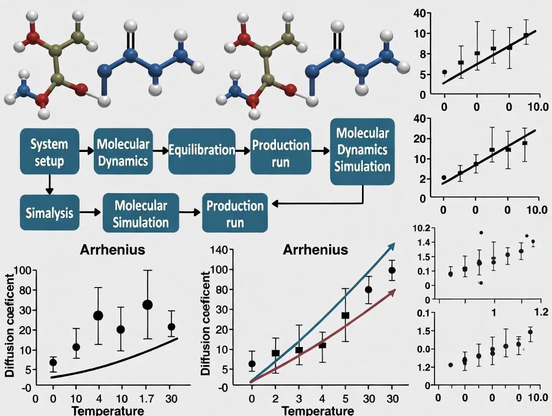
Conceptual Workflow for Diffusion Studies

The following diagram illustrates the logical workflow for applying the Arrhenius equation in a molecular dynamics (MD) study of diffusion, from simulation to final analysis.

Applications in Molecular Dynamics Research

Calculating Diffusion Coefficients from MD Simulations

In Molecular Dynamics (MD) simulations, the diffusion coefficient ( D ) is a primary output used for Arrhenius analysis. It can be calculated primarily through two methods [2].

The Mean Squared Displacement (MSD) method is the most commonly used and recommended approach. It is based on the relationship: ( MSD(t) = \langle [\textbf{r}(0) - \textbf{r}(t)]^2 \rangle ), where ( \textbf{r}(0) ) and ( \textbf{r}(t) ) are the positions of a particle at time zero and time ( t ), respectively, and the angle brackets denote an average over all particles and time origins. For three-dimensional diffusion, the diffusion coefficient is calculated from the slope of the MSD versus time plot in the long-time limit: ( D = \frac{\textrm{slope(MSD)}}{6} ) [2]. It is critical to ensure that the MSD plot is linear, indicating normal diffusive behavior, and to use a sufficiently long simulation time to gather adequate statistics [3] [2].

The Velocity Autocorrelation Function (VACF) method provides an alternative route. The VACF is defined as ( \langle \textbf{v}(0) \cdot \textbf{v}(t) \rangle ), and the diffusion coefficient is obtained from its integral: ( D = \frac{1}{3} \int{t=0}^{t=t{max}} \langle \textbf{v}(0) \cdot \textbf{v}(t) \rangle \rm{d}t ) [2]. This method requires a higher sampling frequency (smaller interval between saved trajectory frames) to accurately capture the velocity correlations.

A key consideration in these simulations is the presence of finite-size effects. The calculated diffusion coefficient can depend on the size of the simulation supercell. A robust approach involves performing simulations for progressively larger supercells and extrapolating the results to the "infinite supercell" limit [2].

MD Protocol for Ion Transport in Solids

The following workflow details the key steps for performing MD simulations to study ion diffusion in solid-state materials, a critical application in battery and fuel cell research.

Table 1: Key Parameters for a Production MD Simulation for Diffusion Studies

Parameter	Typical Setting/Value	Purpose and Rationale
Task	Molecular Dynamics	Defines the type of simulation.
Force Field/Engine	ReaxFF [2] or other ab initio	Determines the interatomic potentials.
Thermostat	Berendsen, Nose-Hoover	Maintains constant temperature.
Total Steps	100,000+ [2]	Ensures sufficient sampling for statistics.
Time Step	0.5 - 2.0 fs	Balances computational efficiency and numerical stability.
Sample Frequency	5-10 steps [2]	Determines output trajectory resolution.
Equilibration Steps	10,000+ [2]	Allows system to reach equilibrium before data collection.

The Scientist's Toolkit: Research Reagent Solutions

Table 2: Essential Materials and Software for MD-based Diffusion Studies

Item	Function/Description	Example from Literature
Molecular Dynamics Software	Platform for running simulations and calculating trajectories.	AMS package with ReaxFF engine [2].
Force Fields	Mathematical functions describing interatomic potentials.	LiS.ff for lithium-sulfur systems [2].
Visualization/Analysis Tools	Software for monitoring simulations and analyzing results.	AMSmovie for viewing trajectories and plotting MSD/VACF [2].
Polymer Matrix	Biodegradable drug carrier material whose properties affect diffusion.	Poly-D,L-lactide-co-glycolide (PLGA) nanoparticles [4].
Model Drug Compound	Fluorescent tracer for monitoring release kinetics.	Rhodamine 6G (R6G) [4].
Solvent	Medium for drug release studies or gas diffusion.	Phosphate buffer (pH 7.4) [4].
Sibenadet	Sibenadet, CAS:154189-40-9, MF:C22H28N2O5S2, MW:464.6 g/mol	Chemical Reagent
2,6-Dibromopyridine	2,6-Dibromopyridine, CAS:626-05-1, MF:C5H3Br2N, MW:236.89 g/mol	Chemical Reagent

Experimental Protocols and Data Analysis

Generating an Arrhenius Plot from MD Data

The process of constructing an Arrhenius plot to extract the activation energy (( Ea )) and pre-exponential factor (( D0 )) involves a clear, step-by-step procedure [2]:

• Perform MD Simulations at Multiple Temperatures: Conduct production MD runs for the same system at a minimum of four different temperatures (e.g., 600 K, 800 K, 1200 K, 1600 K) to establish a reliable temperature trend [2].
• Calculate Diffusion Coefficients (( D )): For the trajectory generated at each temperature, compute the diffusion coefficient using the MSD method, ensuring the MSD plot has a linear region from which a stable slope can be derived [2].
• Transform the Data: For each temperature ( T ), calculate its inverse (( 1/T ), in Kelvin⁻¹). Then, take the natural logarithm of each corresponding diffusion coefficient to get ( \ln(D) ).
• Plot and Fit: Create a plot of ( \ln(D) ) on the y-axis versus ( 1/T ) on the x-axis. The data points should form a straight line if they follow Arrhenius behavior. Perform a linear regression (least squares fit) on the data points.
• Extract Parameters: From the linear fit equation, ( y = mx + c ):
  • Activation Energy (( Ea )): Calculate as ( Ea = -m \times R ), where ( m ) is the slope of the line and ( R ) is the gas constant (8.314 J/mol·K).
  • Pre-exponential Factor (( D0 )): Calculate as ( D0 = e^{c} ), where ( c ) is the y-intercept of the fitted line.

Protocol for Validating Diffusion Data

A critical aspect of reliable MD research is the validation of the simulation data to avoid unsound conclusions [3]. Key validation steps include:

• Confirming Diffusive Behavior: Before calculating ( D ), it is essential to verify that the system has transitioned from subdiffusive to normal diffusive behavior. This is evidenced by a linear regime in the MSD plot [3].
• Optimal Equilibration: The system must be fully equilibrated before starting the production run. The equilibration time should be determined by monitoring the stabilization of properties like energy, pressure, and volume [3].
• Assessing Statistical Accuracy: Running multiple independent simulations or very long trajectories is necessary to ensure that the calculated MSD slope and resulting ( D ) value have converged and are not subject to large statistical uncertainties [2].

Advanced Concepts and Non-Arrhenius Behavior

While the Arrhenius equation is widely applicable, its assumption of temperature-independent ( Ea ) and ( D0 ) is a simplification. State-of-the-art research often deals with non-Arrhenius behavior, where the plot of ( \ln(D) ) vs. ( 1/T ) shows curvature instead of a perfect straight line [5] [6].

Several advanced frameworks address this:

• Modified Arrhenius Equation: A common extension is ( k = A T^n e^{-E_a / RT} ), which includes an explicit power-law dependence on temperature in the pre-exponential factor [1] [5].
• New Functional Forms for Liquid Phases: Recent work has proposed equations with four kinetic parameters to accurately describe the temperature dependence of liquid phase reaction rates from room temperature up to the solvent's critical point, where the original Arrhenius law fails [5].
• Anharmonicity and Temperature-Dependent Activation Energies: In solids, anharmonic vibrations at high temperatures can lead to a temperature-dependent activation energy. For example, in body-centered cubic tungsten, strong anharmonicity explains the observed non-Arrhenius self-diffusion, a finding enabled by ab initio machine-learning approaches [6]. This signifies a paradigm shift from the traditional explanation based on di-vacancies.

The Arrhenius equation remains a cornerstone for interpreting the temperature dependence of diffusion coefficients in MD research. Its application, from setting up and running validated MD simulations to analyzing trajectories via MSD and constructing Arrhenius plots, provides a direct pathway to extract fundamental thermodynamic parameters like the activation energy. However, researchers must be aware of its limitations and the growing evidence of non-Arrhenius behavior in complex systems. The integration of advanced computational frameworks, including machine-learning potentials and anharmonic corrections, is pushing the boundaries of accurate diffusion prediction, offering profound insights for materials science and drug development.

In the study of temperature-dependent phenomena, from chemical reaction rates to molecular diffusion, the Arrhenius equation provides a fundamental framework for understanding the thermal activation processes. Within the specific context of molecular dynamics (MD) research on diffusion coefficients, the two parameters of the Arrhenius equation—the activation energy (Ea) and the pre-exponential factor (D0)—serve as critical indicators of the underlying mechanisms and rates of atomic and molecular transport. This application note details the theoretical significance, experimental determination, and practical application of these key parameters for researchers and scientists engaged in drug development and materials science.

The standard form of the Arrhenius equation for diffusion is expressed as: D = Dâ‚€ exp(-Ea/RT) where D is the diffusion coefficient, Dâ‚€ is the pre-exponential factor (or attempt frequency), Ea is the activation energy for the diffusion process, R is the universal gas constant, and T is the absolute temperature [7] [2]. A more useful linearized form of the equation is used for graphical determination of these parameters: ln(D) = ln(Dâ‚€) - (Ea/R)(1/T) [8] [1] [2]

This relationship reveals that a plot of ln(D) versus 1/T—known as an Arrhenius plot—yields a straight line with a slope of -Ea/R and a y-intercept of ln(D₀) [8] [1]. The careful determination of this plot through MD simulation or experiment is therefore central to extracting these essential kinetic parameters.

Parameter Definitions and Significance

Activation Energy (Ea)

The activation energy (Ea) represents the minimum energy barrier that must be overcome for a diffusion process to occur [8] [1]. In the context of diffusion, it corresponds to the energy required for an atom or molecule to jump between adjacent lattice sites, navigate through amorphous regions of a polymer, or escape from a potential energy well [7] [2].

• Physical Interpretation: Ea reflects the temperature sensitivity of the diffusion process. A higher Ea indicates that the diffusion rate is more strongly dependent on temperature changes [1] [7].
• Theoretical Foundation: The exponential term exp(-Ea/RT) in the Arrhenius equation represents the fraction of atoms or molecules in a system that possess sufficient kinetic energy to surpass the energy barrier Ea at a given temperature T, following the Maxwell-Boltzmann energy distribution [1].

Pre-exponential Factor (Dâ‚€)

The pre-exponential factor (Dâ‚€), also known as the frequency factor or attempt frequency, encompasses the intrinsic characteristics of the diffusing species and the matrix through which diffusion occurs [1] [2].

• Physical Interpretation: Dâ‚€ relates to the number of attempts per unit time that a particle makes to overcome the activation barrier. It is influenced by factors such as the vibrational frequency of the atom in its potential well and the geometry of the diffusion pathway [1] [7].
• Theoretical Foundation: In transition state theory, the pre-exponential factor is related to the entropy change associated with the diffusion process. A higher entropy gain in the transition state corresponds to a larger Dâ‚€ value [1].

Quantitative Parameter Data

The following tables compile representative values of activation energy (Ea) and pre-exponential factor (Dâ‚€) for diffusion processes in various material systems, as reported in recent research.

Table 1: Activation Energies and Pre-exponential Factors for Ag Diffusion in SiC (Silicon Carbide) [9]

Experimental Method	Activation Energy, Ea (kJ·mol⁻¹)	Pre-exponential Factor, D₀
Ag Paste (FBCVD SiC)	247.4	Not Specified
Integral Release (Irradiated TRISO fuel)	125.3	Not Specified
Fractional Ag Release during Irradiation	121.8	Not Specified
Ag Ion Implantation	274.8	Not Specified

Table 2: Exemplary Activation Energies for Gas Permeation in Polymers [7]

Polymer	Permeant	Pre-exponential Factor, P₀ (cm³ mm/m² day atm)	Activation Energy, ΔEp (kJ/mol)
Low Density Polyethylene	Oxygen	5.82 × 10⁹	42.7
Low Density Polyethylene	Nitrogen	2.88 × 10¹⁰	49.9
Low Density Polyethylene	Carbon Dioxide	5.43 × 10⁹	38.9
Poly(vinylidene chloride)	Nitrogen	7.88 × 10¹⁰	70.3
Poly(vinylidene chloride)	Oxygen	7.22 × 10¹⁰	66.6

Table 3: Research Reagent Solutions and Essential Materials for Diffusion Studies

Item	Function/Application
General Purpose Polystyrene (GPPS) / High Impact Polystyrene (HIPS)	Polymer matrix for studying diffusion of organic molecules, relevant to food packaging and drug delivery systems [10].
n-Alkane Model Compounds (e.g., n-octane to n-tetracosane)	A series of surrogate contaminants with varying molecular volumes to systematically study diffusion behavior in polymers [10].
Organic Solvent Mixtures (e.g., Acetone, Ethyl Acetate, Toluene, Chlorobenzene)	Model compounds representing different chemical functionalities for desorption and permeation kinetics studies [10].
ReaxFF Force Field (e.g., LiS.ff)	A reactive force field used in molecular dynamics simulations to model chemical reactions and diffusion in complex systems like lithiated sulfur cathodes [2].
Berendsen Thermostat	An algorithm used in MD simulations to control the temperature of the system, crucial for simulating temperature-dependent diffusion [2].

Experimental Protocols

Molecular Dynamics Protocol for Determining D and Ea

This protocol outlines the procedure for calculating diffusion coefficients (D) at multiple temperatures using molecular dynamics (MD) simulations and subsequently determining the activation energy (Ea) and pre-exponential factor (Dâ‚€) via an Arrhenius plot [2].

Step 1: System Preparation and Equilibration

• Import/Construct the Atomic Model: Build or import the initial atomic structure of the system (e.g., a crystal structure from a CIF file or an amorphous structure).
• Geometry Optimization and Lattice Relaxation: Perform an energy minimization using a conjugate gradient method or similar algorithm to relieve internal stresses and find a low-energy equilibrium configuration. This step often includes optimizing the unit cell dimensions [2].
• Simulated Annealing (For Amorphous Systems): To generate a realistic amorphous structure, perform an MD simulation with a specific temperature profile:
  • Step 1 (5,000 steps): Hold at 300 K.
  • Step 2 (20,000 steps): Heat linearly from 300 K to 1600 K.
  • Step 3 (5,000 steps): Cool rapidly from 1600 K to 300 K [2].
• Re-optimization: Perform a final geometry optimization on the annealed structure.

Step 2: Production MD Simulations at Multiple Temperatures

• Setup: For the equilibrated structure, set up a series of MD simulations (e.g., at 600 K, 800 K, 1200 K, and 1600 K). Using at least four different temperatures is recommended for a reliable Arrhenius plot [2].
• Parameters:
  • Task: Molecular Dynamics.
  • Force Field: Select an appropriate force field (e.g., ReaxFF for reactive systems [2] or COMPASS [11]).
  • Ensemble: NPT (constant Number of particles, Pressure, and Temperature) is commonly used.
  • Thermostat: Use a thermostat like Berendsen with a damping constant of 100 fs to maintain the target temperature [2].
  • Steps: Typically 100,000+ production steps after equilibration.
  • Time Step: 0.25-1.0 fs.
  • Sample Frequency: Save atomic coordinates and velocities every 5-10 steps for subsequent analysis [2].

Step 3: Diffusion Coefficient (D) Calculation from MD Trajectory The diffusion coefficient can be calculated using one of two primary methods:

• A. Mean Squared Displacement (MSD) Method (Recommended)
  • Calculate the MSD for the diffusing species (e.g., Li ions) over time: MSD(t) = ⟨[r(0) - r(t)]²⟩.
  • The diffusion coefficient D is obtained from the slope of the linear region of the MSD plot: D = slope(MSD) / (6) for 3-dimensional diffusion [2]. The divisor is 2d, where d is the dimensionality.
  • Ensure the MSD plot is linear, indicating normal diffusion. A non-linear plot may require a longer simulation time for better statistics [2].
• B. Velocity Autocorrelation Function (VACF) Method
  • Calculate the VACF for the diffusing species: ⟨v(0) · v(t)⟩.
  • The diffusion coefficient D is obtained by integrating the VACF: D = (1/3) ∫₀ᵗᵐᵃˣ ⟨v(0) · v(t)⟩ dt [2].
  • The plot of the integrated value should converge to a constant value for large enough times.

Step 4: Construct Arrhenius Plot and Determine Ea and Dâ‚€

• For each temperature T in your study, you now have a diffusion coefficient D(T).
• Prepare an Arrhenius plot by plotting ln(D) on the y-axis against 1/T (where T is in Kelvin) on the x-axis [8] [2].
• Perform a linear regression (least-squares fit) on the data points. The resulting plot should be a straight line [1].
• Calculate the Parameters:
  • Activation Energy (Ea): From the slope (m) of the fitted line: Ea = -m × R, where R is the universal gas constant (8.314 J·mol⁻¹·K⁻¹) [8] [2].
  • Pre-exponential Factor (Dâ‚€): From the y-intercept (b) of the fitted line: Dâ‚€ = exp(b) [2].

Experimental Laboratory Protocol for Determining Ea of Diffusion in Polymers

This protocol describes an experimental approach based on desorption kinetics to determine diffusion coefficients and activation energies in polymer systems like polystyrene, relevant to drug packaging and functional barriers [10].

Step 1: Sample Preparation and Spiking

• Polymer Sheet Fabrication: Manufacture thin polymer sheets (e.g., ~350 µm thickness) of the material under study (e.g., GPPS, HIPS).
• Homogeneous Spiking: Incorporate a mixture of model compounds (e.g., n-alkanes like n-octane to n-tetracosane, and other organics like toluene, benzophenone) homogeneously into the polymer melt during the sheet formation process [10].
• Concentration Quantification: Determine the initial concentration of each model compound in the spiked sheets using solvent extraction (e.g., with acetone at 40°C for 3 days) followed by GC-FID analysis, or headspace-GC for volatile substances [10].

Step 2: Desorption Kinetics Measurement

• Isothermal Desorption: For each desired temperature (e.g., from 0°C to 115°C), place weighed samples of the spiked polymer (e.g., 1.0 g) into headspace vials [10].
• Headspace Sampling and Analysis: At specific time intervals, analyze the concentration of the model compounds in the headspace of the vials using Headspace Gas Chromatography with Flame Ionization Detection (HS-GC-FID) [10].
  • Typical HS-GC Conditions [10]:
    • Column: ZB-1, 30 m length.
    • Oven Temp.: 50°C (4 min) to 320°C at 20°C/min.
    • HS Oven Temp.: 150°C.
    • Equilibration Time: 1 hour.

Step 3: Diffusion Coefficient (D) Calculation from Desorption Data

• Kinetic Analysis: From the time-dependent decay of the model compound concentration in the polymer (obtained from the headspace signal), determine the desorption kinetics.
• Fickian Diffusion Model: Assuming the desorption follows Fick's laws of diffusion, fit the kinetic data to an appropriate solution of the diffusion equation for the given sample geometry (e.g., a thin sheet) to extract the diffusion coefficient D at each temperature [10].

Step 4: Determine Activation Energy (Ea) and Pre-exponential Factor (Dâ‚€)

• This step is identical to Step 4 of the MD protocol. Plot ln(D) vs. 1/T for the experimentally determined diffusion coefficients and perform a linear fit to obtain Ea and Dâ‚€ from the slope and intercept, respectively [10].

Workflow and Data Analysis Diagrams

Diagram Title: Overall Workflow for Determining Ea and Dâ‚€

Diagram Title: Diffusion Coefficient Calculation Paths

Physical Interpretation of Activation Energy in Diffusion Processes

In the field of materials science and drug development, understanding ion and molecular transport within solid-state materials or biological systems is fundamental for designing better batteries, pharmaceuticals, and drug delivery mechanisms. Molecular Dynamics (MD) simulations have become an indispensable tool for interpreting experimental data, revealing diffusion mechanisms, and predicting the properties of new systems [3]. A critical component of this analysis is the temperature-dependent diffusion coefficient, which often follows an Arrhenius relationship, providing direct access to the activation energy ((E_a)) of the diffusion process.

The physical interpretation of this activation energy is the energy barrier that atoms or ions must overcome to move from one stable site to another within a material or macromolecular structure. This application note, framed within broader thesis research on temperature-dependent diffusion, details the protocols for obtaining this key parameter from MD simulations, providing structured data, experimental methodologies, and visualization tools tailored for researchers and scientists in drug development and materials science.

Theoretical Foundation

Molecular diffusion describes the spread of particles through random motion from regions of high concentration to low concentration. In the context of MD simulations, the self-diffusion coefficient ((D)) can be directly calculated from the mean squared displacement (MSD) of particles over time using the Einstein relation [12]:

[ \langle |\mathbf{r}(t) - \mathbf{r}(0)|^2 \rangle = 2nDt ]

where (\mathbf{r}(t)) is the position at time (t), (\mathbf{r}(0)) is the initial position, (n) is the dimensionality (typically 3 for MD simulations), and the angle brackets denote an ensemble average. The diffusion coefficient is then one-sixth of the slope of the MSD versus time plot [2] [12].

Alternatively, the diffusion coefficient can be obtained through the Green-Kubo relation, which integrates the velocity autocorrelation function (VACF) [2] [12]:

[ D = \frac{1}{3} \int_{0}^{\infty} \langle \mathbf{v}(0) \cdot \mathbf{v}(t) \rangle dt ]

The temperature dependence of the diffusion coefficient is empirically described by the Arrhenius equation [2]:

[ D(T) = D0 \exp\left(-Ea / k_B T\right) ]

where (D0) is the pre-exponential factor representing the theoretical maximum diffusion coefficient at infinite temperature, (Ea) is the activation energy, (kB) is the Boltzmann constant, and (T) is the absolute temperature. By plotting (\ln(D)) against (1/T), one obtains the Arrhenius plot, where the slope is (-Ea/kB), thus allowing for the direct calculation of the activation energy [2]. Physically, (Ea) represents the average energy barrier that a diffusing particle must surmount to hop between stable positions in its local environment.

_{Figure 1: Workflow for extracting activation energy from MD simulations. The key steps involve calculating diffusion coefficients at multiple temperatures and constructing an Arrhenius plot.}

Quantitative Data Presentation

Table 1: Diffusion Coefficient Calculation Methods from MD Simulations

Method	Fundamental Equation	Key Requirements	Advantages	Potential Pitfalls
Mean Squared Displacement (MSD) [2] [12]	( D = \frac{\text{slope}(MSD)}{6} ) ( MSD(t) = \langle [\mathbf{r}(0) - \mathbf{r}(t)]^2 \rangle )	Long simulation times to ensure linear MSD; confirmation of transition from subdiffusive to diffusive behavior [3].	Intuitively clear; directly related to particle trajectories; recommended for its reliability [2].	Finite-size effects require careful supercell size selection and potential extrapolation [2].
Velocity Autocorrelation Function (VACF) [2] [12]	( D = \frac{1}{3} \int{0}^{t{max}} \langle \mathbf{v}(0) \cdot \mathbf{v}(t) \rangle dt )	High sampling frequency (small time between saved velocity frames) for accurate integration [2].	Can provide mechanistic insights into diffusion; may converge faster than MSD in some cases.	Sensitive to the correlation time and the upper limit of integration ((t_{max})).

Table 2: Example Diffusion Coefficients and Extracted Activation Energy for Li0.4S

The following data, extracted from a tutorial on Li_0.4S cathode materials [2], illustrates the process of determining activation energy.

Temperature (K)	Diffusion Coefficient, D (m²/s)	ln(D)	1/T (K⁻¹)
600	To be calculated	-	0.001667
800	To be calculated	-	0.001250
1200	To be calculated	-	0.000833
1600	3.09 × 10⁻⁸ [2]	-17.29	0.000625

Note: The activation energy (E_a) and pre-exponential factor (D_0) are obtained from the linear fit of ln(D) vs. 1/T.

Experimental Protocols

Protocol: Calculation of Diffusion Coefficient via MSD Analysis

This protocol details the steps for computing the diffusion coefficient from a Molecular Dynamics trajectory using the Mean Squared Displacement method, as implemented in the SCM software suite [2].

I. Prerequisites

• A fully equilibrated MD trajectory file (e.g., from a ReaxFF, GAFF, or other force field engine).
• Ensure the trajectory is from the production run (equilibration steps excluded).
• The trajectory should contain atomic positions at a consistent sampling frequency.

II. Step-by-Step Procedure 1. Open the trajectory: Load the completed MD calculation in a visualization/analysis tool like AMSmovie. 2. Select MSD analysis: Navigate to the appropriate analysis menu (e.g., MD Properties → MSD). 3. Set analysis parameters: - Atoms: Specify the atom type for analysis (e.g., Li for lithium ions). - Steps: Define the range of MD steps for analysis, excluding the initial equilibration period (e.g., 2000 - 22001). - Max MSD Frame: Set to a value that ensures the MSD plot is linear, typically corresponding to a time shorter than the total simulation time (e.g., 5000 frames). 4. Generate the MSD plot: Execute the calculation. The software will generate an MSD versus time plot. 5. Calculate D: The diffusion coefficient (D) is one-sixth of the slope of the linear region of the MSD curve. The analysis software often calculates this automatically and displays the value.

III. Critical Validation - Linearity Check: The MSD plot must be linear for the diffusion coefficient to be valid. A non-linear MSD indicates that the system may not be in a diffusive regime or the simulation time is too short [3]. - Convergence Check: The derived D value should be stable and not drift over longer simulation segments.

Protocol: Extrapolation to Lower Temperatures via Arrhenius Plot

This protocol describes how to determine the activation energy and predict diffusion coefficients at temperatures that are computationally prohibitive to simulate directly [2].

I. Prerequisites - Diffusion coefficients ((D)) calculated at a minimum of four different temperatures (e.g., 600 K, 800 K, 1200 K, 1600 K) using the protocol in Section 4.1.

II. Step-by-Step Procedure 1. Prepare data table: Create a table with columns for Temperature (T), calculated D, ln(D), and 1/T. 2. Construct Arrhenius plot: Plot ln(D) on the y-axis against 1/T on the x-axis. 3. Perform linear regression: Fit a straight line to the data points. The equation of the line will be: [ \ln(D) = \ln(D0) - \frac{Ea}{kB} \cdot \frac{1}{T} ] 4. Extract parameters: - Activation Energy ((Ea)): Calculate from the slope ((m)) of the line: (Ea = -m \cdot kB). - Pre-exponential factor ((D0)): Calculate from the y-intercept: (D0 = \exp(\text{intercept})). 5. Extrapolate: Use the fitted Arrhenius equation to predict (D) at any desired temperature (e.g., room temperature, 300 K).

_{Figure 2: Logical workflow for extrapolating diffusion coefficients to lower temperatures using an Arrhenius relation, which allows prediction of properties at experimentally relevant temperatures.}

The Scientist's Toolkit

Table 3: Essential Research Reagent Solutions for MD Simulations of Diffusion

Tool / Reagent	Function / Role	Example Application
Force Fields (e.g., GAFF, ReaxFF)	Defines the potential energy surface governing atomic interactions, including bonded and non-bonded terms.	GAFF has been used to predict diffusion coefficients of organic solutes in aqueous solution with good accuracy [12]. ReaxFF is suitable for simulating lithiated sulfur cathode materials [2].
Simulation Software with MD Engines	Performs the numerical integration of Newton's equations of motion to generate particle trajectories.	Packages like AMS with ReaxFF enable setting up and running MD simulations with defined thermostats and sampling frequencies [2].
Thermostat (e.g., Berendsen)	Controls the system temperature during the simulation by scaling velocities.	Used in simulated annealing protocols (e.g., heating from 300 K to 1600 K and cooling) and production runs at a constant temperature [2].
Structure Builder & Optimizer	Imports, generates, and energetically relaxes initial atomic structures before production MD.	Used to create amorphous Li0.4S structures by inserting Li atoms into a sulfur crystal and performing geometry optimization with lattice relaxation [2].
Trajectory Analysis Tool	Analyzes MD output to compute properties like MSD, VACF, and ultimately the diffusion coefficient.	Tools like AMSmovie are used to generate MSD plots and calculate D from the slope, automating the application of the Einstein relation [2].
Insulin Lispro	Insulin Lispro	Insulin Lispro is a rapid-acting insulin analog for diabetes research. This product is for Research Use Only and is not intended for diagnostic or therapeutic use.
7-Hydroxyquetiapine	7-Hydroxyquetiapine, CAS:139079-39-3, MF:C21H25N3O3S, MW:399.5 g/mol	Chemical Reagent

The Role of Temperature in Atomic and Molecular Jump Mechanisms

Atomic and molecular jump mechanisms are fundamental to understanding diffusion and structural evolution in materials science. Temperature is a critical parameter that governs the kinetics and dynamics of these jumps. This article details the protocols for investigating these mechanisms, with a specific focus on generating data for temperature-dependent diffusion coefficient Arrhenius plots using Molecular Dynamics (MD) simulations. The content is structured to provide researchers with actionable methodologies, validated by recent research, including studies on grain boundary stagnation in polycrystalline materials and diffusion in energy-relevant compounds [13] [2].

Key Concepts and Theoretical Background

Atomic jumps refer to the discrete, thermally activated displacement of atoms or molecules from one stable lattice site to another. These jumps are the elementary steps underlying macroscopic phenomena such as diffusion, creep, and phase transformations.

The Role of Temperature: Temperature provides the thermal energy required for atoms to overcome the energy barriers (activation energy, Ea) separating stable configurations. This relationship is quantitatively described by the Arrhenius equation for the diffusion coefficient (D):

D(T) = D₀ exp(-Eₐ / kBT)

where Dâ‚€ is the pre-exponential factor, kB is the Boltzmann constant, and T is the absolute temperature [2]. A plot of ln(D) against 1/T (an Arrhenius plot) should yield a straight line, from which Eₐ and Dâ‚€ can be extracted.

However, this behavior can be complex. Disruptive atomic jumps, as identified in grain boundary migration, demonstrate non-Arrhenius behavior at high driving forces and temperatures. These are jumps by a few atoms that disrupt the collective, ordered motion of a grain boundary, leading to its stagnation. Crucially, the atoms involved in these disruptive jumps do not differ significantly from their neighbors in terms of local energy, volume, or structure, making them challenging to detect with standard analysis and requiring specialized methods like displacement vector analysis [13].

Experimental Protocols

The following protocols outline the core procedures for using Molecular Dynamics (MD) to study jump mechanisms and compute diffusion coefficients for Arrhenius analysis.

Protocol 1: Calculating Diffusion Coefficients via MD

This protocol is adapted from studies on lithium diffusion in cathode materials and organic molecules in solution [2] [12].

Objective: To compute the diffusion coefficient (D) of a species (e.g., Li+ ions, solvent molecules) at a specific temperature from an MD trajectory.

Procedure:

• System Preparation and Equilibration:
  • Build the System: Import or construct the initial atomic structure. For diffusion in solids, this may involve creating a supercell from a CIF file [2].
  • Equilibrate the System: Perform a geometry optimization followed by MD equilibration in the NVT ensemble (constant Number of particles, Volume, and Temperature) at the target temperature. Use a thermostat like Berendsen with a damping constant of 100 fs. The system must reach equilibrium, confirmed by stable potential energy and temperature [3] [2].
• Production MD Run:
  • Switch to the NVE ensemble (constant Number of particles, Volume, and Energy) or continue in NVT for production data collection.
  • Run a sufficiently long simulation (e.g., 100,000+ steps) to achieve good statistics. The required time depends on the system size and diffusion rate [12].
  • Set the sampling frequency to save atomic coordinates and velocities every few steps (e.g., every 5 steps). The time between saved frames, Δt = (sampling frequency) * (time step), defines the time resolution for analysis [2].
• Diffusion Coefficient Analysis:
  • Mean Squared Displacement (MSD) Method (Recommended):
    • Calculate the MSD for the atoms of interest (e.g., Li) over the production trajectory. The 3D MSD is defined as MSD(t) = ⟨[r(0) - r(t)]²⟩ [2] [12].
    • Plot MSD(t) against time. For normal diffusion, this relationship becomes linear at long times.
    • Perform a linear fit to the MSD curve in the diffusive regime.
    • Calculate the diffusion coefficient using the Einstein relation: D = slope(MSD) / 6 (for 3-dimensional diffusion) [2] [12].
  • Velocity Autocorrelation Function (VACF) Method:
    • Calculate the VACF: <v(0)â‹…v(t)> [12].
    • Integrate the VACF over time to obtain D: D = (1/3) ∫₀^{t_max} <v(0)⋅v(t)> dt [2].

Validation Note: For solutes in solution, reliable prediction of D can require very long simulation times (tens of nanoseconds). Averaging results from multiple independent short-MD simulations is an efficient sampling strategy [12].

Protocol 2: Generating an Arrhenius Plot

Objective: To determine the activation energy (Ea) and pre-exponential factor (Dâ‚€) for a diffusion process.

Procedure:

• Multi-Temperature Simulations: Using the exact same system setup and simulation parameters (except temperature), perform Protocol 1 for at least four different temperatures (e.g., 600 K, 800 K, 1200 K, 1600 K) [2].
• Calculate D(T): For each temperature, compute the diffusion coefficient D using the MSD method.
• Construct the Arrhenius Plot:
  • Create a table of ln(D) and 1/T for all simulated temperatures.
  • Plot ln(D) on the y-axis versus 1/T on the x-axis.
• Linear Regression and Parameter Extraction:
  • Perform a linear fit: ln[D(T)] = ln(D₀) - (Eₐ / k_B) * (1/T).
  • The y-intercept of the fit gives ln(Dâ‚€).
  • The slope of the fit is -Eₐ / k_B, from which the activation energy Eₐ is calculated [2].

Workflow Visualization

The following diagram illustrates the logical workflow for these protocols, from system setup to the final Arrhenius analysis.

Data Presentation and Analysis

Quantitative Data on Temperature-Dependent Phenomena

The table below summarizes key quantitative findings from recent studies on various temperature-dependent atomic and molecular jump mechanisms.

Table 1: Summary of Temperature-Dependent Jump and Diffusion Phenomena

System	Temperature Range	Key Observation / Value	Analysis Method	Reference
Grain Boundary Migration	Various High T	Disruptive atomic jumps cause GB stagnation; Non-Arrhenius behavior observed.	Displacement Vector Analysis	[13]
Li~0.4~S Cathode	600 K - 1600 K	D at 1600 K: ~3.05×10⁻⁸ m²/s (avg. of MSD/VACF). Used for Arrhenius extrapolation.	MSD & VACF	[2]
Carbyne-Graphene Nanoelement	< 1000 K > 1000 K	Strength decreases ~linearly with T; transition to defect-mediated failure.	Strength Calculation	[14]
Rejuvenators in Aged Bitumen	Experimental T range	Diffusion coefficients: 10⁻¹¹ to 10⁻¹⁰ m²/s; Order: Bio-oil > Engine-oil > Naphthenic-oil > Aromatic-oil.	MD Simulation & Experimental Validation	[15]
Organic Solutes in Aqueous Solution	300 K	Average Unsigned Error (AUE) from expt.: 0.137 ×10⁻⁵ cm²/s.	MSD (GAFF Force Field)	[12]

Visualizing the Atomic Jump Mechanism

The following diagram illustrates the mechanism of a disruptive atomic jump at a grain boundary, as revealed by atomistic simulations [13].

The Scientist's Toolkit: Essential Research Reagents and Materials

Table 2: Key Software and Force Fields for MD Simulations of Jump Mechanisms

Item Name	Function / Application	Specific Example / Note
ReaxFF Force Field	Reactive force field for simulating chemical reactions and diffusion in complex materials (e.g., Li-S batteries).	Used with the AMS software package to simulate Li ion diffusion in a Li~0.4~S cathode [2].
General AMBER Force Field (GAFF)	Force field for simulating small organic molecules and their diffusion in solution.	Validated for predicting diffusion coefficients of organic solutes in aqueous solution with high accuracy [12].
TIP4P/2005 Water Model	Rigid, non-reactive water potential for simulating the structure and dynamics of water and ice.	Used to study the structural evolution of amorphous solid water (ASW) upon annealing [16].
AMS Software Package	A unified software suite for performing MD and Monte Carlo simulations with various force fields.	Used in the tutorial for calculating Li ion diffusion coefficients [2].
Displacement Vector Analysis	A specialized analytical method to detect subtle, disruptive atomic jumps that are not revealed by standard metrics.	Critical for identifying the atoms responsible for grain boundary stagnation [13].
Isoluminol	Isoluminol, CAS:3682-14-2, MF:C8H7N3O2, MW:177.16 g/mol	Chemical Reagent
Parogrelil	Parogrelil	Parogrelil is a potent PDE3 inhibitor for research into asthma and circulatory diseases. This product is for Research Use Only (RUO). Not for human use.

Understanding atomic and molecular jump mechanisms through the lens of temperature is vital for advancing materials design and drug development. The protocols detailed here, centered on MD simulations and Arrhenius analysis, provide a robust framework for quantifying these dynamics. Researchers must be aware of complexities such as non-Arrhenius behavior and the subtle nature of disruptive jumps, which necessitate advanced detection methods. The integration of well-validated force fields and careful simulation practices, as outlined, ensures the reliable generation of data that can inform the development of new materials, from battery components to pharmaceutical formulations.

Differentiating Interstitial, Substitutional, and Surface Diffusion Mechanisms

Diffusion in solids is a fundamental transport phenomenon that governs mass transport, phase transformations, and microstructural evolution in a wide range of engineering materials, from structural alloys to functional drug delivery systems. The mechanism and rate of atomic diffusion significantly influence material properties including strength, durability, and corrosion resistance, making understanding these processes essential for materials design and optimization. In crystalline solids, atomic diffusion proceeds through several well-characterized pathways, primarily categorized as substitutional, interstitial, and surface diffusion, each with distinct kinetics influenced by atomic size, bonding, crystal structure, temperature, and defect density. These parameters control both the rate and directionality of atomic motion, dictating which mechanism dominates under a given set of conditions. This application note provides a comprehensive differentiation of these fundamental diffusion mechanisms, with particular emphasis on their characterization through temperature-dependent diffusion coefficients and Arrhenius analysis within molecular dynamics (MD) research frameworks, specifically contextualized for materials and pharmaceutical applications.

Fundamental Mechanisms and Theoretical Framework

Substitutional Diffusion

Substitutional diffusion occurs when atoms migrate by exchanging positions with vacancies within the crystal lattice. This mechanism is typical for larger atoms that occupy regular lattice sites and cannot easily pass through interstitial spaces. The process is governed by two key energy components: the vacancy formation energy, which determines how many vacancies are present, and the migration energy, which defines the barrier for an atom to jump into an adjacent vacant site. Substitutional diffusion is relatively slow due to strong atomic bonding and low vacancy concentrations at low to moderate temperatures. A direct atomic-scale observation of this mechanism was demonstrated in Hf-doped α-Al₂O₃, where Hf atoms were found to preferentially diffuse along grain boundaries by exchanging with co-segregated Al vacancies [17].

Interstitial Diffusion

Interstitial diffusion involves the migration of small atoms (e.g., hydrogen, carbon, nitrogen) through interstitial sites between larger host atoms in the lattice. Since this mechanism does not require vacancies, it occurs at significantly higher rates than substitutional diffusion, often by several orders of magnitude. The activation energy is primarily due to the distortion of surrounding atoms as the interstitial atom squeezes through the lattice. This mechanism is particularly important in processes such as carburization, nitriding, and hydrogen embrittlement phenomena. Body-centered cubic (BCC) structures facilitate faster interstitial diffusion due to their more open lattice, resulting in lower activation energies. Research on ω-TiZr alloys has demonstrated distinct interstitial site preferences for hydrogen atoms, with identified pathways exhibiting energy barriers as low as 0.145 eV for specific site-to-site migrations [18].

Surface Diffusion

Surface diffusion occurs when atoms migrate along the exposed surface of a material, which typically has unsatisfied bonds and higher free energy. This mechanism facilitates rapid atomic transport along defect cores with significantly lower activation energies compared to bulk lattice diffusion. Surface diffusion is critical in processes such as catalysis, sintering, oxidation, and thin-film growth, and becomes particularly dominant in nanostructures, films, and powders where high surface area-to-volume ratios promote rapid atomic mobility. While these mechanisms do not contribute significantly to bulk mass transport in thick materials, they are critically important in nanoscale systems and surface-mediated processes [19].

Mathematical Foundation: Fick's Laws and Arrhenius Equation

Mathematically, diffusion is classically described by Fick's Laws. Fick's First Law models steady-state atomic flux, driven by concentration gradients, while Fick's Second Law captures transient diffusion behavior, showing how concentration profiles evolve over time. These formulations provide the foundation for modelling mass transport in metallurgical and materials systems [19].

The temperature dependence of diffusion is universally described by the Arrhenius equation: $$D = D_0 \exp\left(-\frac{Q}{RT}\right)$$ where D is the diffusion coefficient, D₀ is the pre-exponential factor, Q is the activation energy, R is the gas constant, and T is the absolute temperature. This relationship demonstrates that diffusion rates increase exponentially with temperature, with the activation energy Q representing the energy barrier for the atomic jump process [19]. Molecular dynamics simulations of hydrogen diffusion in tungsten have successfully utilized this relationship, calculating diffusion coefficients from mean squared displacement data and fitting them to the Arrhenius equation to obtain activation energies of 1.48 eV with a pre-exponential factor of 3.2×10⁻⁶ m²/s [20].

Quantitative Comparison of Diffusion Mechanisms

Table 1: Comparative Analysis of Diffusion Mechanisms in Solids

Parameter	Substitutional Diffusion	Interstitial Diffusion	Surface Diffusion
Atomic Mechanism	Exchange with vacancies	Movement through interstitial sites	Migration along surface or defect cores
Typical Activating Species	Larger atoms (Hf in Al₂O₃) [17]	Small atoms (H, C, N in metals) [19]	Adatoms on surfaces (H, O on ω-TiZr) [18]
Activation Energy Range	High (includes vacancy formation + migration)	Low to moderate (primarily migration)	Very low (reduced coordination)
Relative Diffusion Rate	Slowest	Fast (orders of magnitude faster than substitutional)	Fastest (short-circuit path)
Temperature Dependence	Strong (Arrhenius behavior)	Strong (Arrhenius behavior)	Strong (Arrhenius behavior)
Crystal Structure Influence	FCC vs. BCC packing affects vacancy mobility	BCC favored over FCC for interstitial sites	Surface orientation and roughness dependent
Experimental Observation Methods	Time-resolved atomic-resolution STEM [17], Tracer profiling	MD simulations [20], First-principles calculations [18]	First-principles calculations [18], Field ion microscopy

Table 2: Experimentally Determined Diffusion Parameters from Recent Studies

Material System	Diffusing Species	Mechanism	Activation Energy (eV)	Pre-exponential Factor D₀ (m²/s)	Reference
α-Al₂O₃ GB	Hf	Substitutional (vacancy exchange)	Not specified	Not specified	[17]
α-Al₂O₃ GB	Hf	Interstitial (GB)	0.5	Not specified	[17]
Tungsten (BCC)	H	Interstitial	1.48	3.2×10⁻⁶	[20]
ω-TiZr (surface)	H	Surface	0.145 (H3→H2)	Not specified	[18]
ω-TiZr (surface)	O	Surface	0.433 (H3→H4)	Not specified	[18]
ω-TiZr (bulk)	H	Interstitial	0.386 (OC4→OC5)	Not specified	[18]
ω-TiZr (bulk)	O	Interstitial	0.489 (OC4→OC2)	Not specified	[18]

Experimental Protocols and Methodologies

Molecular Dynamics Protocol for Diffusion Coefficient Calculation

The following protocol outlines the procedure for computing diffusion coefficients using molecular dynamics simulations, as demonstrated in studies of lithium ions in Liâ‚€.â‚„S cathode materials [2] and hydrogen in tungsten [20]:

System Preparation:

• Import Crystal Structure: Begin with the crystal structure of the host material, typically imported from a CIF file.
• Insert Dopant/Defect Atoms: Use builder functionality to randomly insert diffusing species atoms (e.g., Li, H) into the host system. For accurate representation, use Grand Canonical Monte Carlo (GCMC) methods for optimal placement.
• Geometry Optimization: Perform energy minimization through geometry optimization including lattice relaxation to achieve a stable initial configuration.
• Simulated Annealing (for amorphous systems): Create amorphous systems through MD-based simulated annealing:
  • Heat system from 300K to high temperature (e.g., 1600K) over 20000 steps
  • Rapid cool-down to room temperature over 5000 steps
  • Use Berendsen thermostat with damping constant of 100 fs

Production MD Simulation:

• Equilibration Phase: Run 10,000-20,000 steps at target temperature to equilibrate system.
• Production Phase: Execute 100,000+ steps for trajectory analysis with appropriate sampling frequency (every 5-100 steps).
• Thermostat Settings: Use Berendsen or Nosé-Hoover thermostat with damping constant of 100 fs for temperature control.

Diffusion Coefficient Calculation:

• Mean Squared Displacement (MSD) Method (Recommended):
  • Calculate MSD from trajectories: $MSD(t) = \langle [\textbf{r}(0) - \textbf{r}(t)]^2 \rangle$
  • Determine diffusion coefficient: $D = \textrm{slope(MSD)}/6$ for 3D systems
  • Ensure MSD plot is linear; if not, extend simulation time for better statistics
• Velocity Autocorrelation Function (VACF) Method:
  • Compute VACF: $\langle \textbf{v}(0) \cdot \textbf{v}(t) \rangle$
  • Integrate to obtain D: $D = \frac{1}{3} \int{t=0}^{t=t{max}} \langle \textbf{v}(0) \cdot \textbf{v}(t) \rangle \rm{d}t$

Arrhenius Analysis:

• Repeat MD simulations at multiple temperatures (minimum 4 points, e.g., 600K, 800K, 1200K, 1600K)
• Plot ln(D) versus 1/T and perform linear fit
• Extract activation energy Eₐ from slope and pre-exponential factor Dâ‚€ from intercept [2]

Direct Atomic-Scale Observation Protocol (STEM)

For direct observation of dopant diffusion at atomic scale, as demonstrated in Hf-doped α-Al₂O₃ [17]:

Sample Preparation:

• Prepare specially oriented samples containing grain boundaries of interest (e.g., Σ31 [0001]/(47Ì…11Ì…0) GB in α-Alâ‚‚O₃)
• Introduce dopant atoms (e.g., Hf) through appropriate doping techniques

Microscopy and Analysis:

• Time-Resolved Atomic-Resolution STEM:
  • Use 300 kV electron probe which provides sufficient energy to overcome diffusion barriers without damaging sample
  • Acquire sequential frames (e.g., 50 frames over 85 seconds) with annular dark-field (ADF) detection
  • Utilize Z-contrast principle for heavy atom identification (Hf atoms appear brighter)
• Statistical Tracking:
  • Construct maximum intensity maps to identify all Hf locations
  • Track Hf atom positions frame-by-frame across multiple datasets (e.g., 3120 frames)
  • Calculate difference images between consecutive frames to identify atomic jumps
• Data Analysis:
  • Categorize diffusion events (substitutional vs. interstitial)
  • Calculate Gibbsian excess to determine GB concentration (e.g., 0.25 ± 0.02 atom nm⁻² for Hf in α-Alâ‚‚O₃)
  • Statistically analyze site preferences and jump frequencies

First-Principles Calculation Protocol

For determining diffusion pathways and energy barriers, as applied to H and O in ω-TiZr alloys [18]:

Calculation Setup:

• Model Construction: Build supercell models of surface and bulk phases with appropriate periodic boundary conditions
• Adsorption Site Analysis: Identify all possible interstitial sites (e.g., H1-H4 on surface, OC1-OC5 in bulk)
• Energy Calculations: Use density functional theory (DFT) with appropriate exchange-correlation functionals

Diffusion Pathway Analysis:

• Transition State Location: Employ nudged elastic band (NEB) method or dimer method to identify minimum energy paths
• Energy Barrier Calculation: Compute activation energies as difference between saddle point and initial state energies
• Site Preference Analysis: Calculate adsorption energies for all identified sites to establish stability hierarchy
• Diffusion Coefficient Estimation: Derive theoretical diffusion coefficients from energy barriers for comparison with experimental values

Visualization of Diffusion Mechanisms and Research Workflows

Diagram 1: Research Workflow for Diffusion Mechanism Identification. This flowchart illustrates the integrated experimental and computational approach for differentiating diffusion mechanisms, highlighting the three primary pathways and characterization methodologies.

Diagram 2: Atomic-Scale Mechanisms of Diffusion. This diagram illustrates the fundamental differences between the three primary diffusion mechanisms at the atomic level, highlighting structural relationships and key characteristics.

The Scientist's Toolkit: Essential Research Reagents and Materials

Table 3: Essential Research Reagents and Computational Tools for Diffusion Studies

Category	Item/Software	Specification/Purpose	Application Examples
Computational Tools	LAMMPS	Molecular Dynamics simulator with various force fields	Hydrogen diffusion in tungsten [20]
	ReaxFF	Reactive force field for complex chemical systems	Li-ion diffusion in Liâ‚€.â‚„S cathode [2]
	DFT Codes (VASP, Quantum ESPRESSO)	First-principles electronic structure calculations	H/O adsorption and diffusion in ω-TiZr [18]
	ANN Potentials	Machine-learning interatomic potentials with DFT accuracy	Hf diffusion in α-Al₂O₃ GB structures [17]
Simulation Support	Bacterial Foraging Optimization (BFO)	Hyperparameter optimization algorithm	Fine-tuning regression models for drug diffusion [21]
	ν-Support Vector Regression (ν-SVR)	Machine learning regression model	Predicting chemical concentrations in 3D space [21]
Experimental Materials	Hf-doped α-Al₂O₃	Model system for GB diffusion studies	Direct observation of substitutional vs interstitial diffusion [17]
	ω-TiZr Alloys	Getter material for surface diffusion studies	H and O adsorption/diffusion measurements [18]
	Tungsten BCC samples	Model for interstitial diffusion	Hydrogen diffusion mechanism analysis [20]
Characterization Equipment	Atomic-Resolution STEM	300kV with ADF detector for time-resolved imaging	Direct observation of atomic jumps at GBs [17]
	Molecular Dynamics Setup	High-performance computing cluster	Temperature-dependent diffusion simulations [20] [2]
4-Chloro-1-naphthol	4-Chloro-1-naphthol, CAS:604-44-4, MF:C10H7ClO, MW:178.61 g/mol	Chemical Reagent	Bench Chemicals
Tolterodine Dimer	Tolterodine Dimer, CAS:854306-72-2, MF:C35H41NO2, MW:507.7 g/mol	Chemical Reagent	Bench Chemicals

Application Notes for Drug Development Professionals

The principles of diffusion mechanisms find direct application in pharmaceutical development, particularly in drug delivery system design. Understanding and controlling molecular diffusion is crucial for developing effective controlled-release formulations where the rate of drug release is governed by diffusion through carrier matrices. Computational hybrid analyses combining mass transfer modeling with machine learning have demonstrated excellent predictive accuracy for drug diffusion in three-dimensional spaces, with ν-Support Vector Regression achieving R² scores of 0.99777 for concentration prediction [21].

Recent advances in diffusion models for small molecule generation, such as the DrugDiff framework, leverage principles of molecular diffusion in latent spaces to generate novel drug-like compounds with targeted properties. These models employ a multi-step denoising process conceptually analogous to atomic diffusion pathways, gradually transforming random noise into structured molecules through iterative refinement steps [22]. The flexibility of this approach allows guidance toward specific molecular properties without retraining the core model, making it particularly valuable for optimizing drug candidates for desired characteristics such as bioavailability, binding affinity, and synthetic accessibility.

For drug delivery system optimization, molecular dynamics simulations can predict diffusion coefficients of active pharmaceutical ingredients through various carrier matrices, enabling rational design of release profiles. The integration of machine learning approaches further enhances predictive capabilities, allowing rapid screening of formulation candidates based on their predicted diffusion characteristics [21]. These computational tools provide valuable insights before experimental validation, potentially accelerating development timelines and reducing costs associated with empirical formulation approaches.

Practical Guide: Calculating Diffusion Coefficients from MD Simulations

Molecular dynamics (MD) simulation is a cornerstone computational technique for studying the dynamic behavior of molecules at an atomic level, operating on timescales from nanoseconds to microseconds [23]. A critical application of MD is the investigation of diffusion processes, which are fundamental to understanding phenomena in chemistry, biology, and materials science, such as drug delivery, membrane transport, and solute mobility. The accuracy of such studies hinges on two foundational choices: the force field, which determines the interatomic potential energy and forces and the ensemble, which defines the thermodynamic conditions of the simulation [24]. This document provides a detailed protocol for configuring MD simulations specifically for calculating diffusion coefficients, framed within a broader thesis on temperature-dependent diffusion and Arrhenius analysis. The Arrhenius equation, ( k = A e^{-Ea / RT} ), formalizes the exponential dependence of a rate process (like diffusion) on temperature, allowing for the extraction of the activation energy ((Ea)) from an Arrhenius plot ((\ln D) vs. (1/T)) [1] [25]. This guide is designed for researchers, scientists, and drug development professionals seeking to perform rigorous and reproducible in silico diffusion studies.

Theoretical Foundation

Molecular Dynamics and Diffusion

Molecular Dynamics simulates the natural motion of atoms and molecules by numerically solving Newton's equations of motion. In this particle-based description, forces calculated from a potential energy function determine how atomic positions and velocities evolve over time [23]. The self-diffusion coefficient ((D)) is a key transport property that quantifies the mean-squared displacement (MSD) of a particle over time. In an MD simulation, (D) can be calculated from the asymptotic slope of the MSD versus time plot using the Einstein relation: [ D = \frac{1}{2d} \lim_{t \to \infty} \frac{d}{dt} \langle | \mathbf{r}(t) - \mathbf{r}(0) |^2 \rangle ] where (d) is the dimensionality (e.g., 3 for a bulk system), (\mathbf{r}(t)) is the position of a particle at time (t), and the angle brackets denote an ensemble average [24].

The Arrhenius Equation in Diffusion Studies

The temperature dependence of the diffusion coefficient typically follows an Arrhenius-like relationship, [ D = D0 e^{-Ea / RT} ] where (D0) is the pre-exponential factor, (Ea) is the activation energy for diffusion, (R) is the gas constant, and (T) is the absolute temperature [1] [26]. By performing simulations at multiple temperatures and calculating (D) for each, one can construct an Arrhenius plot of (\ln D) versus (1/T). The slope of the resulting linear fit is (-E_a / R), from which the activation energy is directly obtained [25]. This provides crucial molecular-level insight into the energy barrier associated with the diffusive process.

Critical Setup Parameters for Diffusion Studies

Force Field Selection

The force field is an empirical potential energy function used to calculate the potential energy (U) of a system as a function of its atomic coordinates. It is paramount for achieving accurate diffusion coefficients [24].

Energy Terms: A typical biomolecular force field consists of bonded and non-bonded terms [24]: [ U(\vec{r}) = \sum{U{bonded}}(\vec{r}) + \sum{U{non-bonded}}(\vec{r}) ] The bonded terms include potentials for bond stretching, angle bending, and torsion angles. The non-bonded terms are most critical for diffusion, as they govern intermolecular interactions and comprise:

• Electrostatics: Modeled by Coulomb's law, (V{Elec} = \frac{qi qj}{4\pi \epsilon0 \epsilonr r{ij}}), a long-range interaction [24].
• van der Waals (vdW) interactions: Most commonly described by the short-ranged Lennard-Jones (LJ) potential, (V_{LJ}(r) = 4\epsilon \left[ \left( \frac{\sigma}{r} \right)^{12} - \left( \frac{\sigma}{r} \right)^6 \right]), where (\sigma) defines the atomic radius and (\epsilon) the well depth [24].

Force Field Classification:

• Class 1 (e.g., AMBER, CHARMM, OPLS): Use harmonic potentials for bonds and angles. They are computationally efficient and widely used for biomolecular simulations, but may lack accuracy for certain properties without careful parameterization [24].
• Class 2 (e.g., MMFF94): Include anharmonic and cross-terms for a more accurate description of vibrational spectra, but are less common in MD [24].
• Class 3 (Polarizable force fields, e.g., AMOEBA, Drude): Explicitly model electronic polarization, which is critical for accurately simulating systems with varying dielectric environments or response to external fields. While more physically accurate, they are computationally more demanding by at least an order of magnitude [24].

Table 1: Comparison of Common Biomolecular Force Fields

Force Field	Class	Common Uses	Combining Rules for LJ	Considerations for Diffusion Studies
AMBER	1	Proteins, DNA	Lorentz-Berthelot	Well-established; good for standard biomolecules.
CHARMM	1	Proteins, Lipids	Lorentz-Berthelot	Good for heterogeneous systems like membrane proteins.
OPLS	1	Proteins, Ligands	Geometric (OPLS)	Often optimized for liquid properties.
GROMOS	1	Proteins	Geometric	Parameterized for consistency with thermodynamic properties.
AMOEBA	3	Ions, Biomolecules	-	Higher accuracy for electrostatic environments; computationally expensive.
CHARMM/Drude	3	Lipids, DNA	-	Improved description of polarizability; slower dynamics may require longer simulations.

Ensemble Selection

The thermodynamic ensemble defines the conserved quantities during the simulation and profoundly influences the system's behavior and the calculated properties [23].

• NVE (Microcanonical Ensemble): Constant Number of particles, Volume, and Energy. This is the natural result of integrating Newton's equations without modification. While physically rigorous, it does not correspond to standard laboratory conditions and the temperature can fluctuate significantly. It is less commonly used for quantitative studies of temperature-dependent diffusion [23].
• NVT (Canonical Ensemble): Constant Number of particles, Volume, and Temperature. This is the most critical ensemble for Arrhenius studies, as it allows for the direct simulation of a system at a specific, controlled temperature. Thermostats (e.g., Nosé-Hoover, velocity rescale) are applied to maintain a constant temperature, which is essential for obtaining the diffusion coefficient (D) at a series of precise temperatures for the Arrhenius plot [27].
• NPT (Isothermal-Isobaric Ensemble): Constant Number of particles, Pressure, and Temperature. This ensemble mimics common experimental conditions most closely. A barostat is used to maintain constant pressure, allowing the simulation box size to adjust. This is particularly important for systems like liquids, where density changes with temperature. For diffusion studies, running NPT simulations at each target temperature before switching to NVT for production can ensure the correct density is achieved.

For a robust Arrhenius analysis, a recommended protocol is to first equilibrate the system's density and pressure in the NPT ensemble, then switch to the NVT ensemble for the production run from which the diffusion coefficient is calculated. This ensures the temperature is strictly controlled for the dynamics being analyzed.

Experimental Protocol for Diffusion Coefficient Calculation

This protocol outlines the steps for setting up and running an MD simulation to calculate the diffusion coefficient of a molecule, such as water, in a bulk system using GROMACS, a widely used MD suite [27].

System Setup and Equilibration

• Obtain Initial Coordinates: Download or generate the molecular structure file in PDB format [27].
• Generate Topology and Coordinates: Use the pdb2gmx command to create the molecular topology (.top) and coordinate (.gro) files, selecting an appropriate force field (see Table 1) when prompted [27].

• Define the Simulation Box: Place the molecule in the center of a periodic box using editconf. A cubic or dodecahedral box is typical.

• Solvate the System: Fill the box with solvent molecules (e.g., SPC, TIP3P, TIP4P water models) using solvate [27].

• Add Ions (Optional): To neutralize the system's charge or achieve a specific ion concentration, use the genion command after preparing a run input file with grompp [27].

• Energy Minimization: Remove any bad contacts and relax the structure using a steepest descent or conjugate gradient algorithm.

• Equilibration:
  • NVT Equilibration: Equilibrate the system at the target temperature (e.g., 300 K) for 100-500 ps.

  • NPT Equilibration: Further equilibrate the system at the target temperature and pressure (e.g., 1 bar) for 100-500 ps to achieve the correct density.

Production Run and Analysis

• Production MD Simulation: Run a sufficiently long simulation in the NVT ensemble to ensure good statistics for the Mean-Squared Displacement (MSD) calculation. The required length depends on the system size and diffusivity.

• Calculate the Diffusion Coefficient:
  • Extract the trajectory for analysis, ensuring molecules are made whole across periodic boundaries.

  • Calculate the MSD using the msd module.

  • Fit the linear portion of the MSD vs. time plot. The 3D self-diffusion coefficient is given by ( D = \frac{1}{6} \times \text{slope} ).

The following workflow diagram summarizes the key steps in this protocol:

Workflow for MD Simulation and Diffusion Analysis

Validation and Reference Data

A critical step in any simulation study is validation against experimental data. For water diffusion, extensive experimental measurements exist across a wide temperature range [26]. The calculated self-diffusion coefficients from your MD simulation can be compared to these reference values to assess the accuracy of your chosen force field and simulation protocol.

Table 2: Experimental Self-Diffusion Coefficients of Water (H₂¹⁶O) at Various Temperatures for Validation [26]

Temperature (°C)	Absolute Temperature (K)	Diffusion Coefficient, D (10⁻⁹ m²/s)
0.0	273.15	1.130
5.0	278.15	1.313
10.0	283.15	1.536
15.0	288.15	1.777
20.0	293.15	2.022
25.0	298.15	2.299
30.0	303.15	2.590
35.0	308.15	2.919
40.0	313.15	3.240

To generate an Arrhenius plot, calculate (\ln D) and (1/T) (in Kelvin) for each temperature from your simulations and the reference data. A linear fit will yield the activation energy, (E_a).

The Scientist's Toolkit

Table 3: Essential Research Reagent Solutions for MD Simulations

Item / Resource	Function / Purpose
Protein Data Bank (PDB)	Source for initial experimental (e.g., X-ray, NMR) biomolecular structures to serve as simulation starting points [27].
GROMACS MD Suite	A robust, open-source software package for performing MD simulations and subsequent trajectory analysis [27].
CHARMM-GUI	A web-based platform that simplifies the process of building complex molecular systems and generating input files for various MD packages, including GROMACS, CHARMM, NAMD, and AMBER [28].
Force Field Parameter Files	Files (e.g., forcefield.itp in GROMACS) containing all necessary parameters (masses, charges, bond constants, LJ parameters) for the chosen force field [24].
Water Models	Pre-parameterized water molecules (e.g., SPC, TIP3P, TIP4P) used to solvate the system and mimic an aqueous environment [24].
Parameter File (.mdp)	A critical input file that specifies all simulation parameters and algorithms (integrator, thermostats, barostats, output frequency, etc.) [27].
Molecular Visualization Tool (e.g., RasMol, VMD)	Software for visually inspecting molecular structures, simulation boxes, and trajectories [27].
Imidaclothiz	Imidaclothiz, CAS:105843-36-5, MF:C7H8ClN5O2S, MW:261.69 g/mol
2,3-Dichloropyridine	2,3-Dichloropyridine

This application note provides a comprehensive framework for setting up molecular dynamics simulations to study diffusion processes and extract Arrhenius parameters. The careful selection of a force field and thermodynamic ensemble, coupled with a rigorous protocol for system preparation, equilibration, and production analysis, is fundamental to obtaining physically meaningful results. Validation against established experimental data for systems like water is a crucial step in building confidence in the simulation methodology. By adhering to these detailed protocols and leveraging the provided toolkit, researchers can conduct robust in silico investigations into the temperature-dependent diffusion of molecules, yielding valuable activation energies that deepen our understanding of dynamic processes in complex systems.

Extracting Mean Squared Displacement (MSD) from Trajectories

Mean Squared Displacement (MSD) analysis is a cornerstone technique for quantifying particle dynamics from trajectory data, serving as a direct gateway to calculating diffusion coefficients. In the context of molecular dynamics (MD) research, establishing a temperature-dependent diffusion coefficient via the Arrhenius equation provides crucial insights into activation energies and fundamental transport mechanisms [20]. This Application Note details a standardized protocol for accurate MSD extraction from molecular trajectories, emphasizing its critical role in temperature-dependent Arrhenius analysis for research in drug development and materials science.

The MSD function quantitatively describes the average squared distance a particle travels over time and is fundamentally connected to the self-diffusion coefficient, D, through the Einstein relation. For normal diffusion in three dimensions, this relationship is given by:

[MSD(\tau) = \langle | \vec{r}(t + \tau) - \vec{r}(t) |^2 \rangle = 6D\tau]

where (\vec{r}(t)) is the particle's position at time t, and (\tau) is the lag time [29] [30]. The slope of the linear region of the MSD plot against lag time is directly proportional to the diffusion coefficient. When studying temperature dependence, this calculated D is used in the Arrhenius equation:

[D = D0 \exp\left(-\frac{Ea}{k_B T}\right)]

where (D0) is the pre-exponential factor, (Ea) is the activation energy for diffusion, (kB) is Boltzmann's constant, and *T* is the absolute temperature [20]. Plotting (\ln(D)) against (1/T) (an Arrhenius plot) allows for the determination of (Ea) and (D_0), which are essential for understanding diffusion mechanisms and predicting molecular behavior under various thermal conditions.

Key Concepts and Data Presentation

Interpreting MSD Profiles for Motion Classification

The functional form of the MSD plot reveals the underlying nature of the particle's motion [29] [31]. The table below classifies the primary modes of diffusion and their characteristic MSD profiles.

Table 1: Classification of diffusion modes based on MSD profile characteristics.

Type of Motion	MSD Functional Form	Anomalous Exponent (α)	Description
Brownian (Normal)	( MSD(\tau) \propto \tau )	α ≈ 1	Linear increase in MSD with lag time; indicative of free, random diffusion.
Subdiffusive	( MSD(\tau) \propto \tau^\alpha )	α < 1	Power-law growth slower than linear; suggests confined motion or diffusion in crowded environments.
Superdiffusive	( MSD(\tau) \propto \tau^\alpha )	α > 1	Power-law growth faster than linear; indicates directed or active transport with a constant drift velocity.
Confined	( MSD(\tau) \propto R^2 )	—	MSD plateaus to a constant value at long lag times, reflecting motion restricted within a radius R.

Essential Reagents and Computational Tools

Accurate MSD analysis requires robust computational tools and properly prepared trajectory data. The following table summarizes key resources.

Table 2: Essential research reagents and software solutions for trajectory analysis and MSD calculation.

Item/Software	Function/Application	Key Feature
GROMACS (gmx msd)	A comprehensive suite for MD simulations and analysis.	Integrated gmx msd command for efficient calculation of diffusion coefficients from unwrapped trajectories [32].
MDAnalysis (EinsteinMSD)	A Python toolkit for analyzing MD simulations and trajectory data.	Provides the EinsteinMSD class with both windowed and FFT-based algorithms for efficient MSD computation [30].
AMS Trajectory Analysis	A standalone program for analyzing trajectories from AMS molecular dynamics.	Computes MSD and can be used for calculating properties like ionic conductivity [33].
LAMMPS	A widely used molecular dynamics simulator.	Used to run simulations and generate trajectories for subsequent MSD analysis (e.g., as in the tungsten study [20]).
Unwrapped Trajectory	The fundamental input data for a correct MSD calculation.	Atomic coordinates must not be wrapped back into the primary simulation cell when passing periodic boundaries [30] [32].

Experimental Workflow and Protocol

The following diagram outlines the core workflow for extracting temperature-dependent diffusion coefficients from MD simulations, from initial system setup to the final Arrhenius analysis.

Figure 1: A high-level workflow for obtaining activation energy from MD simulations via MSD analysis.

Protocol 1: Calculating MSD using GROMACS

This protocol uses the gmx msd module to compute the mean squared displacement and the self-diffusion coefficient [32].

• Trajectory Preparation (Critical): Ensure your trajectory is "unwrapped." Use the gmx trjconv command with the -pbc nojump or -pbc mol flag to prevent atoms from being wrapped back into the primary simulation box as they cross periodic boundaries.
• Run the MSD Calculation: Execute the gmx msd command in your terminal.
  • -f: Input trajectory file.
  • -s: Input topology file.
  • -o: Output file for the MSD data.
  • -beginfit and -endfit: Define the time range (in ps) for the linear fit to the MSD curve. If set to -1, the default is 10% and 90% of the total time, respectively.
  • -trestart: The time interval (ps) for setting new reference points, balancing statistical accuracy and computational cost.
• Interpretation: The gmx msd output provides the MSD plot and prints the self-diffusion coefficient D (and its error estimate) in the terminal, calculated from the slope of the linear fit within the specified region.

Protocol 2: Calculating MSD using MDAnalysis in Python

For users working within a Python ecosystem, MDAnalysis offers a flexible and programmatic approach to MSD calculation [30].

• Setup and Imports: Begin by importing the necessary libraries.

• Load Trajectory and Calculate MSD: Create a universe object and initialize the EinsteinMSD analysis.

• Plotting and Visualization: Visualize the MSD to identify the linear regime.

• Linear Fitting and Diffusion Coefficient Extraction: Select a linear segment from the MSD plot and perform a linear fit to obtain D.

Protocol 3: From MSD to Arrhenius Analysis

This protocol describes the steps to obtain the activation energy after calculating diffusion coefficients at multiple temperatures, as demonstrated in studies of hydrogen in tungsten [20].

• Run Simulations at Multiple Temperatures: Perform independent MD simulations at a series of different temperatures (e.g., 300 K, 400 K, 500 K, ...) while keeping all other parameters constant.
• Extract D(T): For each temperature, use Protocol 1 or 2 to calculate the diffusion coefficient D.
• Construct the Arrhenius Plot: Create a plot of the natural logarithm of the diffusion coefficients, (\ln(D)), versus the inverse of the absolute temperature, (1/T).
• Perform Linear Regression and Extract Parameters: Fit the data points with a straight line.

The following diagram illustrates the detailed computational and analytical steps involved in the core "Calculate and Analyze" phase of the workflow.

Figure 2: The detailed process for calculating the diffusion coefficient from a single trajectory and proceeding to Arrhenius analysis with multiple temperatures.

Critical Considerations for Robust Analysis

• Trajectory Length and Sampling: MSD analysis requires trajectories of sufficient length to capture the relevant dynamics. The linear segment used for fitting must be long enough to provide a reliable estimate of the slope. Excessively long lag times, however, suffer from poor averaging as the number of data points contributing to the MSD average decreases [29] [30]. A log-log plot of MSD vs. Ï„ can help identify the appropriate linear region for fitting [30].

• Localization Uncertainty and Motion Blur: In experimental single-particle tracking (SPT), factors like static error (localization uncertainty) and dynamic error (motion blur during camera exposure) can introduce offsets in the MSD curve. The MSD function should be corrected to: ( MSD(\tau) = 4D\tau + 4\sigma^2 - 8DR\Delta t ), where (\sigma^2) is the variance of the localization uncertainty [31]. While less critical in high-precision MD simulations, these factors are paramount when analyzing experimental data.

• Anomalous Diffusion and Heterogeneity: In complex systems like living cells or crowded polymers, diffusion is often "anomalous," following the power law ( MSD(\tau) = 4D_\alpha \tau^\alpha ). The anomalous exponent (\alpha) differentiates subdiffusion ((\alpha < 1)) from superdiffusion ((\alpha > 1)) [29] [31]. Furthermore, particles may exhibit multiple modes of motion within a single trajectory. In such cases, MSD analysis can be misleading, and advanced methods like Hidden Markov Models or machine learning-based classification are required to segment the trajectory and identify state-specific dynamics [29].

Theoretical Foundation

The Einstein relation is a cornerstone of kinetic theory, establishing a fundamental connection between the microscopic random motion of particles and their macroscopic diffusion coefficient. In the context of molecular dynamics (MD) simulations, this relation provides the primary method for calculating self-diffusivity from particle trajectories [34] [35].

The Einstein formula expresses the Mean Squared Displacement (MSD) as follows: [ MSD(r{d}) = \bigg{\langle} \frac{1}{N} \sum{i=1}^{N} |r{d} - r{d}(t0)|^2 \bigg{\rangle}{t{0}} ] where (N) represents the number of equivalent particles, (r) denotes atomic coordinates, (d) is the dimensionality of the MSD, and the angle brackets indicate averaging over all possible time origins ((t0)) [34].

The self-diffusion coefficient (Dd) is then derived from the slope of the MSD versus time: [ Dd = \frac{1}{2d} \lim{t \to \infty} \frac{d}{dt} MSD(r{d}) ] where (d) is the dimensionality of the diffusion [34]. In three dimensions ((d = 3)), this simplifies to (D = \frac{1}{6} \lim_{t \to \infty} \frac{d}{dt} MSD(t)) [36].

Table 1: Key Equations in Einstein Relation Theory

Equation Name	Mathematical Form	Parameters Description	Application Context
Einstein MSD Definition	( MSD = \langle | \mathbf{x}(t) - \mathbf{x_0} |^2 \rangle )	(\mathbf{x}(t)): position at time t; (\mathbf{x_0}): reference position [36]	Fundamental definition for all diffusion studies
3D Diffusion Coefficient	( D = \frac{1}{6} \lim_{t \to \infty} \frac{d}{dt} MSD(t) )	(D): self-diffusion coefficient; (MSD(t)): mean squared displacement [34]	Standard for 3D molecular dynamics simulations
Stokes-Einstein-Sutherland	( D = \frac{k_B T}{6 \pi \eta r} )	(k_B): Boltzmann constant; (T): temperature; (\eta): viscosity; (r): hydrodynamic radius [35]	Diffusion of spherical particles in liquids with low Reynolds number
Arrhenius Equation	( D = D0 \exp(-Ea / k_B T) )	(D0): pre-exponential factor; (Ea): activation energy; (T): temperature [20]	Temperature dependence of diffusion processes

The temperature dependence of diffusion follows the Arrhenius equation: [ D = D0 \exp(-Ea / kB T) ] where (D0) is the pre-exponential factor, (Ea) is the activation energy, (kB) is Boltzmann's constant, and (T) is temperature [20]. This relationship enables the construction of Arrhenius plots ((\ln D) versus (1/T)) to extract fundamental thermodynamic parameters from MD simulations [20] [37].

Experimental Protocols and Methodologies

MD Simulation Setup for Diffusion Studies

Proper simulation setup is critical for obtaining accurate diffusion coefficients. The following protocol outlines key considerations:

System Preparation:

• Initial Structure: Create a realistic atomic configuration. For crystal systems, place impurity atoms at appropriate interstitial sites (e.g., tetrahedral sites for hydrogen in BCC tungsten) [20].
• Force Field Selection: Choose appropriate potentials (e.g., EAM potential for metal-hydrogen systems) to accurately describe interatomic interactions [20].
• Solvation: For biomolecular systems, solvate using periodic boundary conditions with adequate padding distance (e.g., 4nm around proteins) [37].
• Equilibration: Perform careful equilibration using canonical (NVT) and isothermal-isobaric (NPT) ensembles before production runs [37].

Simulation Parameters:

• Temperature Control: Conduct simulations across a temperature range relevant to the phenomenon of interest (e.g., 1400-2700K for high-temperature diffusion in tungsten) [20].
• Trajectory Length: Ensure sufficient simulation time to observe diffusive behavior, which may range from nanoseconds for small molecules to microseconds for complex systems [37].
• Time Step: Use appropriate integration time steps (typically 1-2 fs for atomic-level simulations) [37].
• Unwrapped Trajectories: Use unwrapped coordinates to correctly compute MSDs, as wrapped coordinates artificially limit displacement calculations [34].

MSD Calculation Implementation

The MSD calculation involves several technical considerations:

Algorithm Selection:

• Windowed Algorithm: The conventional approach averages over all possible time lags (\tau \le \tau{max}), but scales as (N^2) with respect to (\tau{max}) [34].
• FFT-Based Algorithm: Provides (N \log(N)) scaling and is recommended for long trajectories. Requires the tidynamics package in MDAnalysis implementations [34].

Dimensionality Specification:

• MSD can be computed in specific dimensions ('xyz', 'xy', 'xz', 'yz') or along individual axes ('x', 'y', 'z') depending on the system anisotropy [34].

Practical Implementation in MDAnalysis:

GROMACS Implementation:

Data Analysis and Interpretation

Identifying the Diffusive Regime

A critical step in diffusion analysis is identifying the appropriate time range for linear fitting of the MSD plot [34] [38]. The MSD typically exhibits three regimes:

• Ballistic Regime: At short time scales, MSD (\propto t^2) as particle motion is governed by initial velocities with minimal collisions [38].
• Diffusive Regime: At intermediate times, MSD (\propto t) where true random walk behavior emerges [34].
• Saturation Regime: At long times, statistical noise and finite size effects dominate [34].

The diffusion coefficient should be extracted only from the linear diffusive regime. A log-log plot of MSD versus time can help identify this region, where the slope should be approximately 1 [34].

Linear Fitting and Error Estimation

Once the linear regime is identified ((t{start}) to (t{end})), perform linear regression:

For accurate error estimation, the GROMACS msd tool provides error estimates based on the difference between diffusion coefficients obtained from fits over the two halves of the fit interval [39]. The Python module MD2D calculates uncertainties by ensemble averaging of diffusion coefficients from different time intervals [38].

Temperature Dependence and Arrhenius Analysis

To study temperature-dependent diffusion:

• Calculate diffusion coefficients at multiple temperatures
• Plot (\ln D) versus (1/T) (Arrhenius plot)
• Fit to the Arrhenius equation to extract (Ea) and (D0)

Table 2: Example Diffusion Parameters from MD Studies

System	Temperature Range (K)	Activation Energy (Ea)	Pre-exponential Factor (D0)	Reference
Hydrogen in Tungsten	1400-2700	1.48 eV	3.2×10⁻⁶ m²/s	[20]
Methane in Silicalite	Not specified	Not specified	Not specified	[40]
Crambin Unfolding	500-560	Multiple measures	Multiple measures	[37]

Visualization and Workflow Diagrams

MSD to Diffusion Coefficient Workflow

The following diagram illustrates the complete workflow from MD simulation to diffusion coefficient calculation:

MSD Regimes and Temperature Dependence

This diagram illustrates the different MSD regimes and the temperature dependence of diffusion:

Research Reagent Solutions

Table 3: Essential Tools for MSD and Diffusion Analysis

Tool/Software	Type	Primary Function	Application Example
MDAnalysis	Python Library	Trajectory analysis and MSD calculation	Implementation of EinsteinMSD class with FFT acceleration [34]
GROMACS	MD Simulation Suite	Molecular dynamics with built-in MSD analysis	gmx msd command for diffusion coefficient calculation [39]
MD2D	Python Module	Accurate diffusion coefficient determination	Corrects for finite-size effects and identifies ballistic regime [38]
LAMMPS	MD Simulation Code	Large-scale atomic simulations	Hydrogen diffusion in tungsten studies [20]
tidynamics	Python Package	Fast FFT-based MSD calculation	Required for efficient MSD computation in MDAnalysis [34]

Critical Considerations and Best Practices

Common Pitfalls and Solutions

Trajectory Preparation:

• Pitfall: Using wrapped coordinates that artificially limit particle displacements [34].
• Solution: Always use unwrapped trajectories. In GROMACS, use gmx trjconv -pbc nojump; ensure molecules are made whole with -rmpbc yes in gmx msd [34] [39].

Finite-Size Effects:

• Pitfall: Diffusion coefficients from small simulation cells deviate from thermodynamic limits [38].
• Solution: Apply hydrodynamic corrections or extrapolate to infinite system size using the relation ( D(L) = D\infty - \frac{kB T \xi}{6 \pi \eta L} ), where (L) is box size, (\eta) is viscosity, and (\xi) is a constant [38].

Statistical Sampling:

• Pitfall: Insufficient sampling at long time lags leads to noisy MSD and unreliable diffusion coefficients [34].
• Solution: Use the -maxtau option in GROMACS to limit maximum time delta and improve performance [39]. Ensure trajectory length is at least 10 times longer than the fitted time interval [34].

Validation and Error Analysis

Linear Range Selection:

• Validate the linear regime using log-log plots where the slope should be approximately 1 [34].
• When -beginfit and -endfit are set to -1 in GROMACS, fitting automatically uses 10% to 90% of the data range [39].

Error Estimation:

• GROMACS provides error estimates based on the difference between diffusion coefficients from the first and second halves of the fit interval [39].
• For more robust error analysis, use the block averaging method implemented in tools like MD2D, which calculates standard deviations from multiple time intervals [38].

Convergence Testing:

• Verify that diffusion coefficients remain stable with increasing trajectory length.
• Confirm that results are consistent across multiple independent simulation runs.

By following these protocols and considerations, researchers can reliably extract accurate diffusion coefficients from molecular dynamics simulations, enabling meaningful investigation of temperature-dependent diffusion processes across diverse materials and biological systems.

Constructing Arrhenius Plots from MD Data (lnD vs. 1/T)

The Arrhenius equation is a fundamental formula in physical chemistry that describes the temperature dependence of reaction rates, a principle that extends directly to the temperature dependence of diffusion coefficients (D) in molecular dynamics (MD) simulations [1] [25]. For researchers investigating drug transport, protein folding, and materials design, constructing Arrhenius plots from MD data provides crucial insight into the energy barriers governing molecular processes [37] [23]. This protocol outlines a systematic approach for extracting accurate diffusion parameters from molecular dynamics trajectories and translating them into meaningful Arrhenius representations.

The underlying physical principle states that the diffusion coefficient follows the relationship D = D₀exp(-Eₐ/RT), where Eₐ represents the activation energy for diffusion, R is the universal gas constant, T is absolute temperature, and D₀ is the pre-exponential factor [7]. By performing simulations across multiple temperatures and calculating the natural logarithm of the diffusion coefficient (lnD) against the reciprocal of absolute temperature (1/T), researchers obtain a linear relationship whose slope reveals the activation energy [25] [7]. This approach enables quantitative prediction of molecular transport phenomena under various thermal conditions relevant to pharmaceutical development and biomolecular engineering.

Theoretical Foundation

The Arrhenius Equation for Diffusion

The temperature dependence of diffusion coefficients follows an Arrhenius-type relationship, which can be expressed as [7]: D = D₀exp(-Eₐ/RT)

Taking the natural logarithm of both sides transforms this into the linear form used for Arrhenius plots [1] [25]: lnD = lnD₀ - (Eₐ/R)(1/T)

In this formulation:

• D represents the diffusion coefficient at temperature T
• Dâ‚€ is the pre-exponential factor or frequency factor
• Eₐ denotes the activation energy for diffusion (kJ/mol or kcal/mol)
• R is the universal gas constant (8.314 J/mol·K or 1.987 cal/mol·K)
• T is the absolute temperature in Kelvin

The slope of the resulting line in an Arrhenius plot equals -Eₐ/R, while the y-intercept corresponds to lnD₀ [1] [25]. The activation energy Eₐ represents the energy barrier that must be overcome for molecular diffusion to occur, providing crucial insight into the nature of the transport process [7].

Applicability to MD Simulation Data

Molecular dynamics simulations generate atomic-level trajectories from which diffusion coefficients can be calculated using mean squared displacement (MSD) analysis [23]. When MD simulations are conducted at multiple temperatures, they produce the essential data points needed for Arrhenius analysis. The validity of this approach has been demonstrated in studies of protein dynamics and other biomolecular systems [37].

It is important to note that the Arrhenius relationship typically holds over moderate temperature ranges relevant to biological and pharmaceutical applications [37] [7]. Extreme temperatures may induce deviations from linearity due to changes in the dominant diffusion mechanism or system phase transitions [41].

Experimental Protocol

MD Simulation Setup

A robust MD simulation protocol is essential for generating reliable diffusion data for Arrhenius analysis. The following steps outline a standardized approach using the GROMACS simulation package, adapted from established protocols [27]:

System Preparation

• Obtain initial coordinates: Download protein or molecular structure files from the RCSB Protein Data Bank (http://www.rcsb.org/) [27].
• Generate molecular topology: Use pdb2gmx command to convert PDB to GROMACS format and create topology with appropriate force field selection:

• Define simulation box: Create a cubic box with periodic boundary conditions placing the solute at least 1.0 nm from box edges:

• Solvate the system: Add explicit water molecules using the solvate command:

• Neutralize the system: Add counterions to achieve electroneutrality using the genion command [27].

Energy Minimization and Equilibration

• Energy minimization: Run steepest descent or conjugate gradient minimization to remove steric clashes.
• Equilibration phases:
  • Perform canonical ensemble (NVT) equilibration for 100-500 ps to stabilize temperature
  • Conduct isothermal-isobaric ensemble (NPT) equilibration for 100-500 ps to stabilize pressure [37] [27]

Production Simulation

• Run multiple simulations: Execute production MD runs at a minimum of 5-6 different temperatures spanning the range of interest (e.g., 280-320 K for physiological conditions).
• Ensure adequate sampling: Run each simulation for sufficient time to achieve converged diffusion measurements (typically 10-100 ns depending on system size and complexity) [37].
• Maintain consistent parameters: Use identical simulation parameters (timestep, pressure coupling, etc.) across all temperatures except for the temperature setting itself.

Diffusion Coefficient Calculation

The diffusion coefficient is calculated from the production trajectories using the Einstein relation, which connects the mean squared displacement (MSD) of particles to the diffusion coefficient [23]:

• Extract trajectories: Process MD trajectory files to center molecules and remove periodic boundary effects.
• Calculate MSD: For each temperature, compute the MSD from the trajectory using the GROMACS msd utility or similar analysis tool:

• Determine diffusion coefficient: Fit the linear portion of the MSD versus time curve using the relationship: MSD = 2nDt where n is the dimensionality (typically 3 for 3D diffusion), D is the diffusion coefficient, and t is time. The factor 2n becomes 6 for 3D diffusion, so D = MSD/(6t).

Table 1: Example MD Simulation Parameters for Arrhenius Analysis

Parameter	Setting	Rationale
Force Field	OPLS-AA / AMBER / CHARMM	Compatible with biomolecules [37] [27]
Water Model	SPC/E, TIP3P, TIP4P	Explicit solvent for diffusion studies [27]
Temperature Coupling	V-rescale / Nose-Hoover	Maintains target temperature [27]
Pressure Coupling	Parrinello-Rahman	Maintains constant pressure (1 bar)
Timestep	2 fs	Balances accuracy and efficiency [37]
Non-bonded Cutoff	1.0-1.2 nm	Standard for MD simulations
Electrostatics	PME	Handles long-range interactions

Arrhenius Plot Construction

• Compile diffusion data: Tabulate the calculated diffusion coefficients (D) at each simulation temperature (T).
• Transform variables: Calculate lnD and 1/T for each temperature.
• Generate Arrhenius plot: Create a scatter plot of lnD versus 1/T.
• Perform linear regression: Fit the data points with a straight line using least-squares regression.
• Extract parameters: Calculate activation energy from the slope (Eₐ = -slope × R) and the pre-exponential factor from the intercept (Dâ‚€ = exp(intercept)).

Data Analysis and Interpretation

Quantitative Analysis of Arrhenius Parameters

The following example demonstrates the data analysis process using representative MD simulation data for a small protein system, adapted from published studies on temperature-dependent molecular dynamics [37]:

Table 2: Example Diffusion Data from MD Simulations

Temperature (K)	1/T (K⁻¹)	D (10⁻⁶ cm²/s)	lnD
280	0.003571	1.25	-13.59
290	0.003448	1.89	-13.18
300	0.003333	2.75	-12.81
310	0.003226	3.92	-12.45
320	0.003125	5.42	-12.12

Table 3: Calculated Arrhenius Parameters from Linear Regression

Parameter	Value	95% Confidence Interval	Physical Interpretation
Slope (K)	-4115	-3980 to -4250	Determines activation energy
Eₐ (kJ/mol)	34.2	33.1 to 35.3	Moderate diffusion barrier
lnDâ‚€	1.08	0.92 to 1.24	Frequency factor
R²	0.994	-	High linear correlation

The high coefficient of determination (R²) close to 1.0 indicates strong Arrhenius behavior across the temperature range studied [37]. The activation energy of 34.2 kJ/mol falls within the typical range for protein diffusion in aqueous solutions.

Validation and Quality Control

Linearity Assessment: Visually inspect the Arrhenius plot for deviations from linearity, which may indicate changes in diffusion mechanism or simulation artifacts [41].

Statistical Validation:

• Calculate confidence intervals for both slope and intercept using standard linear regression statistics
• Perform residual analysis to identify outliers or systematic errors
• Verify that the correlation coefficient (R) exceeds 0.95 for reliable parameter estimation [37]

Convergence Testing: Ensure MSD calculations show linear behavior over sufficient simulation time, indicating adequate sampling for diffusion coefficient determination [23].

Research Reagent Solutions

Table 4: Essential Materials and Software for Arrhenius-MD Studies

Item	Specification	Function/Purpose
MD Software	GROMACS, NAMD, AMBER, OpenMM	Performs molecular dynamics simulations [27]
Force Fields	CHARMM36, AMBER, OPLS-AA	Defines molecular interactions and energetics [37] [27]
Solvent Models	SPC/E, TIP3P, TIP4P water	Provides explicit solvation environment [27]
Visualization Tools	VMD, PyMOL, Chimera	Trajectory analysis and visualization
Analysis Tools	MDTraj, MDAnalysis, GROMACS utilities	Diffusion coefficient calculation [27]
Plotting Software	Grace, Matplotlib, Gnuplot, Origin	Creates Arrhenius plots and data fitting [37] [27]
Computational Resources	High-performance CPU/GPU clusters	Enables nanosecond-to-microsecond simulations [27] [23]

Workflow Visualization

The following diagram illustrates the complete workflow for constructing Arrhenius plots from MD data:

Arrhenius Plot Construction Workflow

Troubleshooting and Technical Notes

Common Issues and Solutions

Non-linear Arrhenius plots may indicate:

• Inadequate equilibration at one or more temperatures
• System phase transitions within the temperature range
• Changes in diffusion mechanism with temperature
• Insufficient sampling for MSD calculations

Remedies:

• Extend equilibration periods, particularly at temperature extremes
• Verify system stability through potential energy and density monitoring
• Increase simulation duration to improve MSD statistics
• Consider narrower temperature ranges to maintain consistent phase behavior [37] [41]

High uncertainty in parameters often results from:

• Too few temperature points (minimum 5 recommended)
• Narrow temperature range
• Poor convergence in diffusion coefficients

Remedies:

• Increase number of simulated temperatures (7-10 provides robust fitting)
• Widen temperature range where physically appropriate
• Run multiple independent replicas to estimate statistical uncertainty [37]

Advanced Considerations

For systems showing significant curvature in Arrhenius plots, extended models such as the Vogel-Fulcher-Tammann equation or transition-state theory with temperature-dependent activation energy may provide better descriptions of the temperature dependence [41]. Additionally, when studying complex biomolecular systems, ensure that the simulation time scales capture the relevant dynamics for the diffusion process of interest, which may require microsecond-scale simulations for large proteins or crowded environments [23].

This document provides detailed Application Notes and Protocols on diffusion in three systems—hydrogen in metals, water in nanoconfinement, and ion diffusion—framed within a broader thesis on temperature-dependent diffusion coefficient Arrhenius plot molecular dynamics (MD) research. Understanding diffusion coefficients is critical for researchers and scientists working in fields ranging from drug development, where molecular transportation in liquids is key [42], to energy materials, such as solid-state electrolytes [43]. This document summarizes quantitative data into structured tables, outlines detailed experimental protocols, and provides visualizations of workflows and relationships to serve as a practical toolkit for professionals.

Case Study 1: Water in Nanoconfinement

Application Note

The behavior of water under nanoconfinement is critical for applications in drug delivery, water desalination, and understanding biological ion channels [44] [45] [46]. Under confinement, water's self-diffusion coefficient (D) deviates from its bulk value due to interactions with solid interfaces and geometric constraints. Molecular dynamics (MD) simulations reveal that the self-diffusion coefficient for nanoconfined water scales linearly with a single parameter, θ, which represents the ratio between the confined and total water volumes [45]. The relationship is expressed as:

D(θ) = DB[1 + (DC/D_B - 1)θ]

where DB is the bulk diffusion coefficient and DC is the totally confined diffusion coefficient [45]. This scaling relationship holds across diverse systems, including silica nanopores, nanoparticles, carbon nanotubes, and proteins [45]. Furthermore, the choice of water model in MD simulations is crucial; polarizable models (e.g., AMOEBA) can yield significantly different wetting/de-wetting behaviors in hydrophobic nanopores compared to rigid fixed-charge models [46].

Experimental & Computational Protocol

Objective: To compute the self-diffusion coefficient of water in a nanoconfined environment using molecular dynamics simulations.

Table 1: Key Research Reagent Solutions for Nanoconfined Water Studies

Reagent/Material	Function/Description	Example Specifications
Water Models	Represents water molecules in MD simulations.	TIP4P/2005 [44], SPC, SPC/E, TIP3P, TIP4P, TIP5P [42], Polarizable AMOEBA [46]
Nanoconfining Structure	Provides the nanoscale environment for confinement.	Hydrophobic slit pores or nanotubes [44], SiO2 nanopores [45], TMEM175 ion channel protein [46]
Force Fields	Defines interaction potentials for MD simulations.	OPLS4 [42], GROMOS96 43a2 [45], Lennard-Jones potentials [45]
Software Tools	Performs MD simulations and trajectory analysis.	Schrödinger Materials Science Suite [42], Desmond [42]

Procedure:

• System Preparation: a. Obtain or generate the atomic structure of the confining system (e.g., a silica nanopore, carbon nanotube, or ion channel protein) [45]. b. Embed the structure in a simulation box. For biological channels, this involves placing it within a lipid bilayer membrane [46]. c. Solvate the system with water molecules. The water density should be sufficient to avoid anomalous low-filling behavior [45]. d. Add ions to achieve the desired physiological or experimental salt concentration (e.g., ~0.15 M NaCl) [46].

• Equilibration Simulation: Perform a multi-stage equilibration process to stabilize the system [42]: a. Brownian Dynamics: Run at 10 K for 100 ps with a 1 fs time step. b. NVT Ensemble MD: Use a Langevin thermostat at 10 K for 100 ps with a 2 fs time step. c. NVT Ensemble MD at Target Temperature: Use a Langevin thermostat at the temperature of interest for 100 ps with a 2 fs time step. d. NPT Ensemble MD: Use a Nose-Hoover thermostat and a Martyna-Tobias-Klein barostat at the temperature of interest and 1.01325 bar (1 atm) for 20 ns with a 2 fs time step.

• Production Simulation: Run a final MD simulation in the NPT ensemble for a duration sufficient to gather good statistics for diffusion. For water, 40 ns may suffice for highly diffusive samples, while 150 ns is recommended for lowly diffusive systems [42].

• Trajectory Analysis - Diffusion Coefficient Calculation: a. Mean Squared Displacement (MSD) Method (Recommended): i. Calculate the MSD of the water molecules' center-of-mass from the production trajectory. ii. The self-diffusion coefficient D is given by one-sixth of the slope of the MSD versus time in the linear regime: ( D = \frac{\text{slope(MSD)}}{6} ) [2] [42]. iii. Perform a linear regression (e.g., using the least-squares technique) on the MSD plot over an appropriate lag time range (e.g., 12 to 20 ns for fast diffusion) [42]. b. Velocity Autocorrelation Function (VACF) Method: i. Calculate the VACF from the atomic velocities saved during the production run. ii. Integrate the VACF over time and divide by 3 to obtain D: ( D = \frac{1}{3} \int{0}^{t{\text{max}}} \langle \mathbf{v}(0) \cdot \mathbf{v}(t) \rangle dt ) [2].

Data Presentation and Analysis

Table 2: Experimentally Determined and Simulated Self-Diffusion Coefficients of Pure Liquids (Excerpt) [42]

Liquid	Temperature (K)	Experimental D (10⁻⁹ m²/s)	Simulated D (10⁻⁹ m²/s)	Water Model / Force Field
Water	298	2.60 (Bulk Reference)	Varies with model	TIP3P, TIP4P, OPLS4, etc.
(Other liquids from database)	...	...	...	OPLS4

Table 3: Self-Diffusion Coefficient of Water in Various Nanoconfined Geometries [45]

Confinement Geometry	Key Parameter	Diffusion Coefficient D (10⁻⁹ m²/s)
Bulk Water (Reference)	N/A	2.60
SiO₂ Nanopore	Diameter: 11.0 nm	2.50 ± 0.09
SiO₂ Nanopore	Diameter: 2.0 nm	0.82 ± 0.22
SiO₂ Nanopore (8.1 nm) with 16 Fe₃O₄ NPs	High nanoparticle concentration	0.44 ± 0.05

Case Study 2: Ion Diffusion in Solid Electrolytes

Application Note

Fast ion conductors are pivotal for high-performance solid-state rechargeable batteries. Investigations into materials like pyrochlore-type lithium lanthanum niobium oxyfluoride (Li₂–ₓLa₍₁₊ₓ₎/₃□₍₂ₓ–₁₎/₃Nb₂O₆F) reveal high ionic conductivity originating from fast Li⁺ ion diffusion [43]. The diffusion coefficient (D) of these ions can be directly measured using pulsed-field gradient nuclear magnetic resonance (PFG-NMR). Analysis of the temperature dependence of D via an Arrhenius plot (( \ln{D} ) vs. ( 1/T )) is standard practice. A bending in the Arrhenius plot at a specific temperature (e.g., ~200 K) can suggest an order-disorder phase transition of the Li⁺ ions within the crystal structure, a phenomenon corroborated by changes in the thermal expansion coefficient [43]. Such insights are invaluable for designing superior solid electrolytes.

Experimental & Computational Protocol

Objective: To determine the Li⁺ ion diffusion coefficient in a solid electrolyte material (e.g., Li₀.₄S) using MD simulations and to extrapolate to lower temperatures.

Table 4: Key Research Reagent Solutions for Ion Diffusion Studies

Reagent/Material	Function/Description	Example Specifications
Solid Electrolyte	Material through which ions diffuse.	Pyrochlore-type Oxyfluoride [43], Liâ‚€.â‚„S [2]
Force Field	Defines atomic interactions in MD.	ReaxFF [2]
Characterization Tool	Experimentally measures diffusion coefficient.	Pulsed-Field Gradient NMR (PFG-NMR) [43]

Procedure (Computational - MD for Liâ‚€.â‚„S [2]):

• System Generation: a. Import/Generate Structure: Import a crystal structure (e.g., from a CIF file) or generate an amorphous structure. b. Insert Ions: Use builder tools or Grand Canonical Monte Carlo (GCMC) to insert Li atoms into the structure to achieve the desired stoichiometry (e.g., Liâ‚€.â‚„S). c. Geometry Optimization: Perform a geometry optimization with lattice relaxation using an appropriate force field (e.g., ReaxFF) to equilibrate the structure.

• Creating Amorphous Systems (Optional): To model amorphous materials, perform simulated annealing via MD: a. Heat the system from 300 K to a high temperature (e.g., 1600 K) over a defined number of steps. b. Rapidly cool the system back to room temperature (e.g., 300 K). c. Relax the resulting amorphous structure with another geometry optimization including lattice relaxation.

• Production MD for Diffusion: Run an MD simulation at the target temperature (e.g., 1600 K) for a sufficient number of steps (e.g., 100,000 production steps) with a defined sampling frequency to save atomic positions and velocities.

• Diffusion Coefficient Analysis: Calculate the diffusion coefficient (D) for Li ions using either the MSD or VACF method, as described in Section 2.2.

• Arrhenius Extrapolation: To estimate D at lower temperatures (e.g., 300 K) without running prohibitively long simulations: a. Perform production MD simulations and calculate D for at least four different elevated temperatures (e.g., 600 K, 800 K, 1200 K, 1600 K). b. Create an Arrhenius plot of ( \ln(D(T)) ) versus ( 1/T ). c. Fit the data to the Arrhenius equation: ( \ln{D(T)} = \ln{D0} - \frac{Ea}{kB} \cdot \frac{1}{T} ), where ( Ea ) is the activation energy and ( D_0 ) is the pre-exponential factor. d. Use the fitted parameters to extrapolate D to the lower temperature of interest.

Data Presentation and Analysis

Table 5: Li⁺ Ion Diffusion Coefficient in Pyrochlore-type Oxyfluoride via PFG-NMR [43]

Material	Temperature (K)	Diffusion Coefficient D (m²/s)	Note
Li₂–ₓLa₍₁₊ₓ₎/₃□₍₂ₓ–₁₎/₃Nb₂O₆F	Variable	Measured via PFG-NMR	Bending in Arrhenius plot at ~200 K

Case Study 3: Hydrogen in Metals

Application Note

While the provided search results do not contain a specific case study on hydrogen diffusion in metals, they highlight a relevant and impactful discovery process in energy-related materials science. The search for alternatives to iridium, a rare and expensive metal used as a catalyst in the oxygen evolution reaction (OER) for clean hydrogen production, is a critical challenge [47]. A powerful new tool, the "megalibrary," has been developed to accelerate materials discovery. Each megalibrary contains millions of uniquely designed nanoparticles on a single chip, functioning as a high-throughput "data factory" [47]. This approach enabled researchers to screen vast combinations of abundant and inexpensive metals (ruthenium, cobalt, manganese, chromium) and rapidly identify a new quaternary composition (Ru₅₂Co₃₃Mn₉Cr₆ oxide) that matched or exceeded iridium's OER performance at a fraction of the cost [47]. This case study exemplifies the modern, accelerated approach to discovering and optimizing functional materials, a paradigm that can be directly applied to finding new metal alloys or composites for enhanced hydrogen storage and transport.

The Scientist's Toolkit

Table 6: Essential Research Reagent Solutions for Diffusion Studies

Category	Item	Brief Function/Explanation
Computational Tools	Molecular Dynamics (MD) Software	Simulates the physical movements of atoms and molecules over time. Essential for computing diffusion coefficients from first principles.
	Force Fields	Defines the potential energy surface for atomic interactions. Critical for simulation accuracy (e.g., OPLS4 for liquids, ReaxFF for materials) [2] [42].
	Water Models	Represents water molecules in simulations. Choice (e.g., TIP4P/2005, SPC/E, polarizable AMOEBA) significantly impacts results, especially in confinement [44] [42] [46].
Experimental Techniques	Pulsed-Field Gradient NMR	A primary experimental method for measuring self-diffusion coefficients in liquids and solids [42] [43].
Materials & Platforms	Megalibrary	A high-throughput platform containing millions of nanoparticles on a chip. Used for rapidly discovering new functional materials, such as OER catalysts [47].
Theoretical Frameworks	Stokes-Einstein Relation	Relates the diffusion coefficient to viscosity. A modified "confined" version may be needed for nanoconfined systems [44].
	Arrhenius Equation	Describes the temperature dependence of diffusion coefficients, allowing for the calculation of activation energies [2].
2,5-Diphenyloxazole	2,5-Diphenyloxazole, CAS:92-71-7, MF:C15H11NO, MW:221.25 g/mol	Chemical Reagent
Woodward's reagent K	Woodward's reagent K, CAS:4156-16-5, MF:C11H11NO4S, MW:253.28 g/mol	Chemical Reagent

Addressing Computational Challenges and Non-Arrhenius Behavior

Optimizing Simulation Time and System Size for Statistical Accuracy

Molecular dynamics (MD) simulations are a powerful tool for investigating atomic-scale processes, such as temperature-dependent diffusion in solids. The reliability of the results, particularly for calculating thermodynamic and kinetic properties like diffusion coefficients for Arrhenius plots, depends critically on two factors: the size of the simulated system and the duration of the simulation. Inadequate choices for either can lead to results that are not statistically significant, rendering subsequent conclusions unreliable. This application note provides detailed protocols for optimizing these parameters to ensure the statistical accuracy of your MD research, framed within the context of diffusion studies.

The Critical Role of Statistical Accuracy in MD Simulations

MD simulations, by their nature, sample thermodynamic ensembles and are subject to statistical fluctuations. Assessing the magnitude of these fluctuations by assigning uncertainties to computed results is critical for drawing statistically reliable conclusions [48]. A failure to properly assess this error can lead to erroneous interpretation of simulation data [48].

The core challenge is that observables calculated from poorly converged simulations may appear to show trends, such as a dependence on simulation box size, that disappear with adequate sampling [48]. For instance, the apparent box-size dependence of solvation free energies vanishes when a sufficient number of simulation repeats (e.g., N=20) are performed, highlighting that anecdotal evidence from single or few realizations can be misleading [48]. Therefore, reporting confidence intervals for estimated observables is a fundamental practice for avoiding unfounded claims [48].

Establishing Statistical Confidence

Monitoring Convergence and Uncertainty

• Convergence Monitoring: A statistical approach to MD validation involves monitoring the convergence of simulations to equilibrium. This process involves tracking summary statistics that correspond to experimentally measured quantities over time to ensure they have stabilized [49].
• Confidence Intervals: Once convergence is suspected, obtaining confidence intervals for these summary statistics is essential. These intervals provide a range of values within which the true value of the observable is likely to fall, given the statistical uncertainty of the finite simulation [49].
• Out-of-Sample Prediction: A robust approach to validation and improvement of simulations is based on out-of-sample prediction, often measured by cross-validation. This technique helps ensure that the parameterization of a simulation is not over-fitted to a specific system but can generalize to others [49].

Simulation-Based Sample Size Determination

For complex systems, a general framework for determining sufficient sampling exists. It uses Gaussian Process (GP) regression as a surrogate model to approximate the underlying power function of the statistical test, informed by Monte Carlo simulations [50]. This method is particularly valuable when optimizing several design parameters (like number of clusters and cluster size in multilevel systems) subject to conflicting criteria.

Table: Key Statistical Concepts for MD Validation

Concept	Description	Application in MD
Confidence Intervals [49]	A range of values that likely contains the true value of a population parameter.	Report for calculated observables (e.g., diffusion coefficient, free energy) to show statistical uncertainty.
Cross-Validation [49]	A technique for assessing how the results of a analysis will generalize to an independent data set.	Validate and improve force-field parameters by testing their predictive power on molecules not used in parameterization.
Gaussian Process Regression [50]	A non-parametric Bayesian method for modeling an unknown function.	Efficiently optimize simulation-based sample size and design parameters without exhaustive, costly simulations.

Optimizing System Size

The System Size Trade-Off

The simulation system size must balance two competing factors: computational efficiency and statistical precision. Larger systems generally provide higher precision in predictions but result in longer simulation times [51]. The primary goal is to select a system size that is large enough to avoid finite-size effects that manifest as inaccurate and imprecise predictions, yet small enough to allow for feasible simulation times and adequate sampling [51].

Practical Guidelines and Quantitative Findings

A systematic study on an epoxy resin system provides concrete guidance. It aimed to determine the optimal MD model size that balances predictive precision and simulation cost [51]. The results demonstrated that precision, as measured by the standard deviation of predicted properties, converges as the model size increases.

Table: Effect of MD System Size on Precision and Cost for a Polymer System [51]

Number of Atoms	Key Findings on Precision	Simulation Time Consideration
5,265 - 14,625	Standard deviation of predicted properties reduces as model size increases.	Smaller systems simulate faster but may sacrifice precision.
~15,000 Atoms	Optimal size for the tested epoxy resin, providing the fastest simulations without sacrificing precision for mass density, elastic properties, strength, and thermal properties.	Optimal balance of efficiency and precision.
40,000 Atoms	Convergence for elastic modulus, glass-transition temperature (Tg), and yield strength was observed in a different epoxy system study [51].	Larger systems require more computational resources.

The key takeaway is that the optimal system size is system-dependent, but a methodology exists to find it. For the epoxy resin studied, a size of 15,000 atoms was optimal, while other studies have found convergence at 1,600 atoms for glasses or 40,000 atoms for different epoxy properties [51]. A general rule is to ensure the simulation box is sufficiently large so that the minimal distance between the solute surface and the box edge is at least 1 nm to avoid artifacts from periodic image interactions [48].

Optimizing Simulation Time and Replicates

The Challenge of Statistical Convergence

Achieving statistical convergence is one of the most significant challenges in MD, especially for systems with a large conformational space like intrinsically disordered proteins. Without convergence, the estimated thermodynamic and kinetic properties will have a substantial associated error [52] [48]. The required simulation time is problem-dependent. For instance, reconstructing conformational ensembles for IDRs may require theoretically milliseconds of simulation time to visit each state sufficiently, which is often computationally prohibitive [52].

Strategies for Efficient Sampling

• Enhanced Sampling Techniques: Methods like Replica Exchange Solute Tempering (REST) are considered reference-quality for achieving accurate statistical sampling in complex systems like IDRs [52]. These techniques enhance phase space exploration and help overcome free energy barriers.
• Multiple Independent Replicates: Running several independent simulations (replicates) from different initial conditions is a common and effective strategy. A study on system size effects used five independent replicates for each system size to enable statistical sampling and calculate standard deviations [51]. This approach helps ensure that results are not biased by a single, potentially trapped trajectory.
• Sequential and Adaptive Methods: For determining the number of replicates, a sequential probability ratio test (SPRT) can be used as a stopping rule [53]. This method involves continuously testing a hypothesis (e.g., that a p-value is below a certain threshold) as more data is collected, and stopping only when statistical confidence is reached. This avoids pre-defining an arbitrary number of runs.

Table: Methods for Improving Sampling Efficiency

Method	Principle	Use Case
Multiple Replicates [51]	Running independent simulations from different initial conditions.	Standard practice for obtaining statistical averages and errors for any MD system.
Replica Exchange (REST) [52]	Running multiple replicas at different temperatures or Hamiltonians and allowing exchanges.	Sampling complex landscapes (e.g., protein folding, IDR ensembles).
Markov State Models (MSM) [52]	Clustering many short simulations to build a model of state-to-state transitions.	Extracting long-timescale kinetics from ensembles of shorter, more feasible simulations.
Sequential Probability Ratio Test [53]	Using a statistical test after each new replicate to decide if sufficient data has been collected.	Adaptive determination of the required number of simulation replicates.

Application Protocol: Diffusion Coefficient Calculations

The following protocol is tailored for calculating statistically robust, temperature-dependent diffusion coefficients for Arrhenius analysis (plotting ln(D) vs. 1/T), based on established guidelines [20] [3].

System Preparation and Equilibration

• Build the System: Construct an initial crystal structure (e.g., BCC for tungsten) and insert impurity atoms (e.g., hydrogen) at realistic lattice sites [20].
• Define the Force Field: Select an appropriate potential (e.g., EAM for metal-hydrogen systems [20]).
• Minimization: Perform energy minimization using a method like the conjugate-gradient algorithm to remove high-energy clashes [51].
• Equilibration in the NPT Ensemble: Equilibrate the system at the target temperature and pressure (e.g., 1 atm) using a thermostat/barostat (e.g., Nose-Hoover). Critical Step: The equilibration time must be determined by monitoring the stabilization of key properties like potential energy, temperature, and density [3]. Do not use a fixed, arbitrary time.

Production Run and Analysis

• Production Simulation: Run the simulation in the NVT or NVE ensemble. The simulation must be long enough to observe a clear transition from sub-diffusive to diffusive behaviour in the mean squared displacement (MSD) plot [3].
• Calculate Mean Squared Displacement (MSD): Use the Einstein relation to calculate the MSD of the diffusing species as a function of time [20].
• Extract the Diffusion Coefficient: The diffusion coefficient D is obtained from the slope of the linear region of the MSD curve vs. time, using the formula: D = (1/(6N)) × lim_{t→} d(MSD(t))/dt, where N is the number of diffusing particles [20].
• Repeat at Different Temperatures: Perform simulations across a range of temperatures (e.g., 1400 K to 2700 K [20]).
• Generate Arrhenius Plot and Fit: Plot ln(D) against 1/T and fit the data to the Arrhenius equation, D = Dâ‚€ exp(-Eₐ/(k_B T)), to obtain the activation energy Eₐ and pre-exponential factor Dâ‚€ [20].

The Scientist's Toolkit: Essential Research Reagents and Materials

Table: Key Materials and Software for Reliable MD Simulations of Diffusion

Item Name	Function / Purpose	Example(s)
MD Simulation Engine	Software to perform the numerical integration of Newton's equations of motion.	LAMMPS [51] [20], GROMACS [48]
Force Field	A set of empirical functions and parameters describing interatomic potentials.	EAM (for metals [20]), AMBER [49], Interface Force Field (IFF) [51]
Thermostat/Barostat	Algorithms to control temperature and pressure during the simulation, maintaining the correct thermodynamic ensemble.	Nose-Hoover thermostat/barostat [51] [20]
Analysis Tools	Software or scripts for post-processing trajectory data to compute observables like MSD and diffusion coefficients.	Built-in tools in LAMMPS, GROMACS; custom scripts in Python/MATLAB.
Enhanced Sampling Algorithms	Advanced simulation techniques to improve sampling of rare events and complex energy landscapes.	Replica Exchange Solute Tempering (REST) [52], Hamiltonian Replica Exchange [48]
Betahistine	Betahistine for Research|Histamine Receptor Ligand	High-purity Betahistine for lab research. Explore its role as a histamine H1 agonist/H3 antagonist in vestibular studies. For Research Use Only. Not for human consumption.
Picrolonic acid	Picrolonic Acid: Research-Grade Reagent for Metal Analysis	High-purity Picrolonic Acid for research applications in metal determination, lanthanide extraction, and analytical chemistry. For Research Use Only. Not for human use.

Managing Elevated Temperature Simulations and Vacancy Concentrations

In molecular dynamics (MD) research on temperature-dependent diffusion, the accurate calculation and management of vacancy concentrations at elevated temperatures is a fundamental challenge. The equilibrium concentration of point defects, particularly vacancies, governs atomic diffusion in solids, and their formation energetics directly influence the Arrhenius plot of diffusion coefficients. In pure metals near their melting point, this concentration typically ranges from 10⁻⁴ to 10⁻³ [54]. However, in concentrated solid solutions like high-entropy alloys, the problem becomes complex due to local chemical ordering and anharmonic effects, which are significant at temperatures above the Debye temperature. This document outlines application notes and detailed protocols for simulating vacancy thermodynamics, enabling reliable prediction of diffusion behavior within Arrhenius-based research frameworks.

Theoretical Background and Key Quantities

The equilibrium concentration of a vacancy defect, ( C{\text{vac}} ), is governed by its Gibbs energy of formation, ( G{\text{vac}}(T) ), according to the canonical expression: [ C{\text{vac}} = \exp\left(-\frac{G{\text{vac}}(T)}{kB T}\right) ] The Gibbs energy is temperature-dependent and is defined as ( G{\text{vac}}(T) = H{\text{vac}}(T) - T S{\text{vac}}(T) ), where ( H{\text{vac}} ) is the formation enthalpy and ( S{\text{vac}} ) is the formation entropy [54].

A critical challenge is that self-interstitial atoms (SIAs) generally exhibit substantially higher formation enthalpies than vacancies, leading to equilibrium concentrations that are two or more times lower than vacancy concentrations across a wide temperature range [54]. This makes vacancies the primary mediators of diffusion.

Table: Key Thermodynamic Properties of Point Defects from MD Studies

Property	Material System	Reported Value/Range	Temperature Dependence
Vacancy Concentration	Pure Metals (near melting point) [54]	10⁻⁴ – 10⁻³	Strong (increases with T)
Vacancy Concentration	VNbMoTaW HEA (1000-2700 K) [54]	Between pure V and W values	Weak dependence
SIA Concentration	VNbMoTaW HEA [54]	>2x lower than vacancies	Weak dependence
Vacancy Formation Enthalpy	VNbMoTaW HEA [54]	Significant	Affected by local chemical order
Vacancy Migration Barrier	Tungsten [55]	~1.4 eV (MD), ~1.73 eV (DFT)	-

Computational Methods and Protocols

Direct Molecular Dynamics for Defect Concentration

Principle: This method involves running extensive MD simulations of a large supercell at the target temperature and directly counting the number of thermally generated vacancies or self-interstitial atoms after the system reaches equilibrium [54].

Detailed Protocol:

• Model Construction: Create an atomistic supercell of your material using an appropriate software package (e.g., LAMMPS). The supercell must be large enough to accommodate a statistically meaningful number of defects.
• Equilibration: Run an NPT (constant Number of particles, Pressure, and Temperature) ensemble simulation to equilibrate the system's volume and density at the target temperature and pressure.
• Production Run and Defect Analysis:
  • Perform a long NPT MD simulation (e.g., several nanoseconds) to allow the concentration of self-point defects (SPDs) to reach equilibrium [54].
  • The concentration of vacancies, ( C{\text{vac}} ), is calculated as the ratio of vacant lattice sites, ( N{\text{vac}} ), to the total number of sites in the perfect lattice, ( N ): ( C{\text{vac}} = N{\text{vac}} / N ).
  • Similarly, the concentration of self-interstitial atoms, ( C{\text{i}} ), is the ratio of atoms in interstitial positions, ( N{\text{i}} ), to the total number of lattice sites: ( C{\text{i}} = N{\text{i}} / N ).
• Application Note: This method is computationally demanding as it requires simulating large systems for long times to achieve good statistics for the inherently low defect concentrations. It is most effective at high temperatures, close to the material's melting point.

Gibbs-Helmholtz Integration Method

Principle: This is a more accurate approach for determining the Gibbs energy of vacancy formation, ( G_{\text{vac}}(T) ), by integrating the Gibbs-Helmholtz equation using enthalpy data obtained from MD simulations [54].

Detailed Protocol:

• Enthalpy Calculation via Supercell Approach:
  • Perform MD simulations on two systems: a perfect crystal and a crystal containing a single vacancy (supercell approach).
  • Calculate the formation enthalpy, ( H{\text{vac}}(T) ), at a series of temperatures ( Tj ) above the Debye temperature. The formation enthalpy is the difference in enthalpy between the defective and perfect supercells.
• Gibbs Energy Integration:
  • The Gibbs-Helmholtz equation is given by ( \frac{G(T)}{T} = \frac{G(T0)}{T0} - \int{T0}^{T} \frac{H(T')}{T'^2} dT' ), where ( T0 ) is a reference temperature.
  • To solve this, the integration constant ( G(T0)/T0 ) must be determined. This can be achieved by performing a high-temperature MD simulation where the equilibrium vacancy concentration, ( C{\text{vac}}^{\text{high-T}} ), is measured directly. The constant is then calculated as ( G(T0)/T0 = -\ln(C{\text{vac}}^{\text{high-T}}) / kB ) [54].
  • Numerically integrate the equation using the calculated ( H{\text{vac}}(T) ) data and the constant to obtain ( G{\text{vac}}(T) ) across the desired temperature range.
• Application Note: This method explicitly accounts for anharmonic effects and provides a full thermodynamic description. It is particularly valuable for concentrated alloys where local chemical ordering can significantly impact defect energetics, a effect neglected in simpler statistical models [54].

Hybrid MD/Kinetic Monte Carlo (kMC) for Irradiation Damage

Principle: Under irradiation, microstructural evolution involves timescales inaccessible to standard MD. A hybrid method propagates fast degrees of freedom (interstitial diffusion, cascade collisions) with MD and accelerates the slow, rate-limiting vacancy migration using a kMC scheme [55].

Detailed Protocol:

• MD Phase: Run standard MD to introduce collision cascades (e.g., via simulated recoils) and allow fast-moving interstitial defects to migrate and recombine.
• kMC Phase: Periodically, the simulation is paused. All vacancies in the system are identified. The migration energy barrier for each vacancy is calculated on-the-fly. A kMC step is performed to move one vacancy, advancing the system clock by a time ( \Delta t = -\ln(\xi) / \sumi ki ), where ( \xi ) is a random number and ( k_i ) are the rates of all possible vacancy migration events [55].
• Iteration: The atomic positions are updated after the kMC jump, and the simulation returns to the MD phase. This cycle repeats.
• Application Note: This parameter-free method is powerful for simulating microstructural evolution (void formation, loop growth) at experimentally relevant dose rates and moderately elevated temperatures where vacancy diffusion becomes active [55].

Machine Learning Interatomic Potentials (MLIPs) for Complex Defects

Principle: Machine-learned interatomic potentials trained on Density Functional Theory (DFT) data enable nanosecond-scale MD simulations of complex defect dynamics with near-DFT accuracy, a scale inaccessible to direct DFT-MD [56].

Detailed Protocol:

• Potential Generation: Select an MLIP framework (e.g., Gaussian Approximation Potential (GAP) or MACE). Generate a training set of atomic structures that encompass relevant defect configurations (single vacancies, clusters, line defects) and their pathways [56].
• Training and Validation: Train the MLIP on energies and forces from DFT calculations. Critically evaluate the potential's performance by comparing its predictions for defect migration barriers (e.g., using Nudged Elastic Band method) against pure DFT calculations [56].
• Application: Use the validated MLIP to perform large-scale, nanosecond MD simulations of systems with high vacancy concentrations or complex defect clusters to observe cooperative phenomena, such as the formation of extended line defects [56].
• Application Note: MLIPs are particularly useful for materials like MoSâ‚‚, where vacancy mobility is highly cooperative and depends strongly on the local atomic environment [56]. They bridge the accuracy of DFT and the scale of classical MD.

The Scientist's Toolkit: Research Reagent Solutions

Table: Essential Computational Tools for Vacancy Simulation Studies

Tool Category	Specific Example	Function and Application
Simulation Package	LAMMPS [54]	A widely used, open-source MD simulator that can implement various interatomic potentials and compute thermodynamic properties.
Interatomic Potential	N-body potentials [54]	Empirical potentials parameterized to reproduce key properties like melting point, lattice parameter, and point defect energies.
Interatomic Potential	Machine-Learned Interatomic Potentials (MLIPs) [56]	Potentials (e.g., GAP, MACE) offering near-DFT accuracy for large-scale MD simulations of complex defect dynamics.
Ab Initio Code	Density Functional Theory (DFT) Codes	Used for calculating accurate formation energies and migration barriers and for generating training data for MLIPs [56].
Acceleration Method	Hybrid MD/kMC scheme [55]	A computational protocol to accelerate slow vacancy dynamics, enabling simulation of microstructural evolution at engineering timescales.
Analysis Method	Gibbs-Helmholtz Integration [54]	A thermodynamic integration method to compute the Gibbs energy of vacancy formation from MD-derived enthalpy data.
Analysis Tool	Nudged Elastic Band (NEB) [56]	A computational technique for finding the minimum energy path and the energy barrier for defect migration events.

Identifying and Interpreting Non-Arrhenius (Non-linear) Behavior

Quantitative Data on Non-Arrhenius Behavior

The following table summarizes key characteristics and quantitative indicators used to identify and interpret non-Arrhenius behavior in temperature-dependent diffusion studies.

Table 1: Characteristics and Identification of Non-Arrhenius Behavior

Aspect	Classical Arrhenius Behavior	Non-Arrhenius Behavior	Quantitative Indicators
Mathematical Form	Linear relationship in ln(k) vs. 1/T plot [8]	Curvature in ln(k) vs. 1/T plot [57]	Negative curvature in Arrhenius plot; Non-constant apparent activation energy [57]
Activation Energy	Constant single activation energy (Ea) [8]	Temperature-dependent apparent activation energy [57]	Ea decreases with increasing temperature [57]
Underlying Mechanism	Single energy barrier [8]	Distribution of site energies; Temperature-dependent short-range order [57]	Broad continuous distribution of interstitial site energies [57]
Example Systems	Ideal crystalline solids	Amorphous metals (e.g., TiCuH1.41, Zr2PdHx) [57]	Hydrogen in amorphous Fe–H alloy [57]

Table 2: Experimental Evidence for Non-Arrhenius Diffusion

System Studied	Experimental Technique	Observed Deviation	Proposed Interpretation
Hydrogen in amorphous Fe–H alloy [57]	Computer simulation/modeling	Negative curvature in Arrhenius plot [57]	Related to temperature dependence of short-range order [57]
Hydrogen in amorphous metals [57]	NMR measurements	Non-Arrhenius character [57]	Occupancy of wide variety of interstitial sites with varying energies [57]
Amorphous metals [57]	Monte-Carlo simulations	Pronounced negative curvature [57]	Distribution of site energies (related to trapping) [57]

Experimental Protocols

Protocol: Identifying Non-Arrhenius Behavior in Diffusion Studies

Purpose: To experimentally distinguish between classical Arrhenius and non-Arrhenius temperature dependence of diffusion coefficients.

Materials and Equipment:

• High-purity sample material (e.g., amorphous metal alloy)
• Precision temperature control system (±0.1 K stability)
• Diffusion measurement apparatus (e.g., NMR spectrometer, permeation cell)
• Data acquisition system
• Computational software for data analysis

Procedure:

• Sample Preparation:
  • Prepare or acquire amorphous metal samples (e.g., Fe–H alloy)
  • Ensure sample homogeneity and characterize short-range order using radial distribution function analysis [57]
  • Mount sample in measurement cell ensuring minimal external stress

• Temperature-Dependent Measurements:

  • Set initial temperature (typically lowest point in range of interest)
  • Measure diffusion coefficient using appropriate technique (e.g., hydrogen permeation, tracer diffusion)
  • Increment temperature systematically across wide range (≥100°C recommended)
  • Allow sufficient equilibration time at each temperature (minimum 30 minutes)
  • Repeat measurements at least triplicate at each temperature

• Data Analysis:

  • Plot natural logarithm of diffusion coefficient (ln D) against inverse temperature (1/T)
  • Perform linear regression analysis for entire dataset
  • Calculate residual sum of squares to quantify deviation from linearity
  • If curvature observed, segment data and calculate apparent activation energy for different temperature ranges
  • Compare temperature dependence of activation energy with theoretical models

Expected Outcomes: Non-Arrhenius behavior manifests as systematic curvature in Arrhenius plot with correlation coefficient <0.99 for linear fit. Apparent activation energy decreases with increasing temperature.

Troubleshooting:

• If scatter dominates curvature, increase measurement precision or replicate points
• If temperature range too narrow, extend to wider interval
• Verify temperature calibration and measurement accuracy

Protocol: Computational Modeling of Non-Arrhenius Diffusion

Purpose: To simulate and interpret non-Arrhenius diffusion behavior using physics-informed computational approaches.

Materials and Software:

• High-performance computing cluster
• Molecular dynamics simulation software (e.g., LAMMPS, GROMACS)
• Monte-Carlo simulation package
• Data analysis tools (Python, MATLAB)

Procedure:

• System Setup:
  • Construct amorphous metal model with realistic short-range order
  • Define distribution of interstitial site energies based on radial distribution function [57]
  • Implement distribution of saddle-point energies for transition states

• Simulation Parameters:

  • Set temperature range spanning experimental conditions
  • Use minimum 10,000 atoms for representative sampling
  • Implement appropriate ensemble (NVT or NPT) with reliable thermostat
  • Run minimum 1 nanosecond production runs for each temperature

• Analysis Methodology:

  • Track mean square displacement of diffusing species
  • Calculate diffusion coefficients from slope of MSD vs. time
  • Plot Arrhenius relationship and quantify curvature
  • Correlate diffusion behavior with temperature-induced structural changes
  • Compare with experimental data for validation

Interpretation Guidelines:

• Negative curvature suggests dominant role of site energy distribution [57]
• Temperature-dependent activation energy indicates structural evolution with temperature [57]
• Consistent deviation across multiple simulation runs confirms non-Arrhenius behavior

Visualization of Non-Arrhenius Behavior Concepts

Signaling Pathways and Conceptual Framework

Conceptual Framework for Non-Arrhenius Diffusion

Experimental Workflow for Identification

Experimental Identification Workflow

The Scientist's Toolkit: Research Reagent Solutions

Table 3: Essential Materials and Computational Tools for Non-Arrhenius Studies

Tool/Reagent	Function/Application	Specifications
Amorphous Metal Alloys	Model system for studying non-Arrhenius behavior [57]	High-purity Fe–H, TiCuH1.41, Zr2PdHx systems [57]
NMR Spectrometer	Measurement of hydrogen diffusion coefficients [57]	High-field magnet with variable temperature control
Monte-Carlo Simulation Code	Modeling diffusion in energy landscape with distributed sites [57]	Custom algorithms for site and saddle-point energy distributions [57]
Radial Distribution Function Analysis	Characterization of short-range order in amorphous metals [57]	X-ray or neutron diffraction with pair distribution function analysis
Physics-Informed Machine Learning	Optimization of measurement protocols and parameter estimation [58]	Neural networks incorporating diffusion-relaxation MRI physics [58]

Addressing Statistical Errors in Diffusion Barriers from MD

Molecular dynamics (MD) simulations have become an indispensable tool for calculating diffusion coefficients and extracting diffusion barriers via Arrhenius analysis. However, these derived diffusional properties are often plagued by statistical uncertainties originating from the inherent limitations of MD simulations. Unlike experimental measurements with enormous sampling, MD simulations are constrained to nanoscale systems and picosecond-to-nanosecond timescales, resulting in limited observation of diffusion events. This fundamentally limits the statistical significance of calculated properties [59]. Furthermore, research indicates that uncertainty in MD-derived diffusion coefficients depends not only on the simulation data itself but also on the analysis protocol employed—including choices of statistical estimator, fitting windows, and data processing methods [60]. Without proper accounting of these error sources, researchers risk reporting statistically insignificant diffusion barriers or drawing incorrect conclusions about diffusion mechanisms. This application note provides a comprehensive framework for identifying, quantifying, and mitigating statistical errors when determining diffusion barriers from MD simulations.

Fundamental Limitations of MD Simulations

The statistical power of diffusion properties derived from MD simulations is fundamentally constrained by several computational factors:

• Limited sampling of diffusion events: Ab initio MD (AIMD) simulations typically capture only a limited number of ion hops due to short timescales (picoseconds to nanoseconds), leading to significant statistical variances in calculated diffusivity [59].
• Finite-size effects: The number of molecules used in typical MD simulations is orders of magnitude lower than in the thermodynamic limit, necessitating corrections to computed diffusivities [61].
• Short simulation trajectories: Even with classical MD, insufficient sampling time can result in MSD curves that haven't reached the linear regime, violating key assumptions of linear regression analysis [61].

Analysis Protocol Dependencies

Uncertainty in estimated diffusion coefficients depends critically on analytical choices rather than just the underlying simulation data [60]:

• Statistical estimator selection: Choices between ordinary least squares (OLS), weighted least squares (WLS), and generalized least squares (GLS) regression can yield different uncertainty estimates from the same MSD data.
• Fitting window extent: The selection of which time interval (Δt) to use for linear fitting of the MSD curve significantly impacts the derived diffusion coefficient.
• Time-averaging approaches: Different methods for processing the raw trajectory data before MSD calculation can introduce systematic variations in results.

Table 1: Key Statistical Error Sources in MD-Derived Diffusion Barriers

Error Category	Specific Source	Impact on Diffusion Barrier
Sampling Limitations	Limited diffusion events	High variance in D at each temperature
	Short trajectory length	Non-linear MSD region fitting
	Small system size	Finite-size effects on diffusivity
Analysis Decisions	Regression method choice	Underestimation of confidence intervals
	MSD fitting window selection	Systematic bias in D values
	Equilibration time determination	Non-equilibrium effects on statistics
Physical System	Temperature range width	Extrapolation error in Arrhenius plot
	Insufficient temperature points	Uncertainty in activation energy slope

Experimental Protocols for Robust Diffusion Analysis

Mean Squared Displacement (MSD) Protocol

The most common approach for calculating diffusion coefficients from MD trajectories involves MSD analysis:

• Trajectory preparation: Run production MD simulations with sufficient length to observe multiple diffusion events. For ab initio MD, this may require tens to hundreds of picoseconds depending on the system [59].

• MSD calculation: Compute the mean squared displacement using the Einstein relation:

  • Extract atomic positions ráµ¢(t) throughout the trajectory
  • Calculate MSD(Δt) = (1/N)Σ⟨|ráµ¢(t+Δt) - ráµ¢(t)|²⟩ averaged over all time origins [59]
  • For reliable statistics, ensure the MSD plot reaches a clear linear regime before fitting

• Linear fitting:

  • Select an appropriate fitting window in the diffusive regime (avoiding short-time ballistic and long-time saturation regions)
  • Perform linear regression: MSD(Δt) = 2dDΔt, where d is dimensionality
  • Calculate diffusion coefficient D from the slope: D = slope/(2d) [2]

• Statistical validation:

  • Conduct multiple independent simulations with different initial conditions [61]
  • Verify that MSD curves show linear behavior over significant portion of trajectory
  • Check that derived diffusion coefficient D plateaus rather than drifts with time

Uncertainty Quantification Protocol

To obtain reliable error estimates for diffusion coefficients:

• Multiple trajectory approach: Conduct several independent simulations (recommended: ~40 for good statistics [61]) with different initial velocities.

• Block averaging: Divide a long trajectory into multiple blocks and calculate D for each block to estimate variance.

• Bayesian methods: Use Bayesian regression to sample the distribution of linear models compatible with the MSD data, providing statistically efficient estimates of D and associated uncertainty [61].

• Error propagation: For Arrhenius parameters, propagate uncertainties from individual D(T) values to the final activation energy using standard error propagation formulas.

The diagram below illustrates the complete workflow for robust diffusion coefficient calculation:

Research Reagent Solutions for Diffusion MD

Table 2: Essential Computational Tools for Diffusion MD Studies

Tool Category	Specific Examples	Function in Diffusion Analysis
MD Engines	LAMMPS [20], AMS [2]	Perform molecular dynamics simulations with various force fields
Analysis Packages	VASP [62], Python libraries	Trajectory analysis, MSD calculation, and statistical processing
Force Fields	EAM potentials [20], ReaxFF [2], BOP [62]	Describe interatomic interactions for different material classes
Uncertainty Quantification	Bayesian regression tools [61], Block averaging scripts	Statistical analysis of diffusion coefficients and error estimation
Visualization	AMSmovie [2], OVITO, VMD	Trajectory inspection and diffusion pathway identification

Case Studies and Validation Approaches

Successful Implementation Examples

Several recent studies demonstrate proper approaches to addressing statistical errors in MD-derived diffusion barriers:

• In studying hydrogen diffusion in tungsten, researchers performed molecular dynamics simulations across a temperature range (1400K to 2700K), calculated diffusion coefficients from MSD data, and fitted to the Arrhenius equation to obtain statistically meaningful activation energy parameters [20].

• Research on Zn tracer diffusion in α-Cu₆₄Zn₃₆ combined experimental measurements with MD simulations, showing Arrhenius behavior with an activation enthalpy of 1.37 eV from both approaches, validating the computational methodology [63].

• A hybrid DFT and bond-order potential (BOP) study of H diffusion in Cu grain boundaries used larger supercells (over 900 atoms) to eliminate periodic-image artifacts and enable better statistics for diffusion barrier calculations [62].

Statistical Validation Methods

To ensure the reliability of derived diffusion barriers:

• Convergence testing: Verify that diffusion coefficients do not change significantly with longer simulation times or larger system sizes.

• Goodness-of-fit metrics: For Arrhenius plots (lnD vs. 1/T), report R² values and confidence intervals for the fitted activation energy.

• Residual analysis: Check for systematic patterns in residuals from linear fits to MSD curves and Arrhenius plots.

• Cross-validation: Compare results from different analysis methods (MSD vs. VACF) and from independent simulation replicates [2].

By implementing these protocols and validation strategies, researchers can significantly improve the statistical reliability of diffusion barriers derived from molecular dynamics simulations, leading to more robust conclusions about atomic-scale transport mechanisms in materials.

The accurate prediction of material stability and reaction kinetics is a cornerstone of pharmaceutical development and materials science. Traditional models, particularly the classical Arrhenius equation, have provided a fundamental framework for understanding temperature-dependent reaction rates. However, the complexity of modern drug formulations and biological systems, which are influenced by multiple interacting factors such as humidity, excipient composition, and complex degradation pathways, often renders the traditional model insufficient. This has driven the development of more sophisticated kinetic models, primarily the Modified Arrhenius Equation and the Stretched Exponential Model, which offer enhanced predictive power for complex, real-world systems. Within the context of thesis research on temperature-dependent diffusion coefficients and Arrhenius plots in molecular dynamics (MD), these models provide critical tools for bridging atomic-scale simulations with experimental observables. This note details the application of these advanced models, providing structured data, experimental protocols, and visual workflows to guide researchers and drug development professionals.

Quantitative Model Comparison

The following table summarizes the core characteristics, applications, and quantitative findings for the two advanced kinetic models discussed in this protocol.

Table 1: Comparison of Advanced Kinetic Models

Model Feature	Modified Arrhenius Equation	Stretched Exponential (KWW) Model
Fundamental Form	ln k = a - (E_a/R)(1/T) + b*(%RH) + c*(%Excipient) [64]	f(t) = exp[-(t/τ)^β] [65] [66]
Key Parameters	Activation Energy (Ea), Pre-exponential factor (A), and coefficients for humidity, excipient content, etc. [64]	Characteristic Relaxation Time (τ), Stretching Exponent (β, 0 < β ≤ 1) [65]
Primary Application	Predicting chemical reaction rates (e.g., drug nitrosation, degradation) in multi-factor environments [64] [67]	Describing non-exponential relaxation, aging, and misfolding in disordered systems and proteins [65] [66]
Representative β Value	Not Applicable (N/A)	β = 3/7 (Universal for metallic glass aging at T < Tg) [65]
Representative System	Desloratadine nitrosation in solid dosage forms [64]	Metallic glasses (Zr70Cu30, La60Ni15Al25) [65]
Thesis Context (MD)	Parameterizing coarse-grained models from experimental data; validating simulated diffusion coefficients.	Directly fitting simulation data from protein folding or glassy relaxation trajectories [66].

Experimental Protocols

Protocol for Constructing a Modified Arrhenius Model

This protocol is adapted from studies on drug nitrosation and degradation kinetics [64] [67].

Objective: To develop a modified Arrhenius equation that predicts the reaction rate constant (k) based on temperature, relative humidity (%RH), and alkaline excipient (AE) content.

Materials:

• Model Compound: e.g., Desloratadine (DES) [64]
• Reactant: Sodium nitrite [64]
• Excipients: Alkaline excipient (e.g., Sodium carbonate monohydrate), filler (e.g., D-mannitol, crystalline cellulose) [64]
• Stability Chambers: To control temperature and relative humidity [64]
• Analytical Instrumentation: High-Performance Liquid Chromatography (HPLC) system for quantitative analysis [64]

Procedure:

• Sample Preparation: Prepare physical mixtures (PMs) of the model drug, nitrite, and excipients. Systematically vary the alkaline excipient content (e.g., 0.0% to 10% w/w) while keeping other components constant [64].
• Stability Study Design:
  • Temperature & Humidity Variation: For a fixed AE content, expose PM samples to a matrix of different temperatures (e.g., 50°C, 60°C, 70°C) and relative humidity levels (e.g., 20%RH, 40%RH, 60%RH) [64].
  • Excipient Content Variation: At a fixed temperature and humidity, study PMs with different AE content levels [64].
• Kinetic Measurement: At predetermined time intervals, remove samples and quantify the concentration of the reaction product (e.g., N-nitroso desloratadine, NDES) using HPLC [64]. Determine the apparent reaction rate constant (k) at each condition from the slope of the concentration-time profile.
• Data Analysis & Model Construction:
  • Perform multiple regression analysis using the least-squares method on the collected k values against the independent variables (1/T, %RH, %AE) [64].
  • The resulting model will take a form similar to: ln k = 41.38 - 13026 × (1/T) + 0.038 × (%RH) - 0.44 × (% w/w(AE)) [64].
  • Validate the model by comparing its predictions against experimental data from a long-term stability study not used in the model construction [64].

Protocol for Analyzing Stretched Exponential Kinetics

This protocol is derived from research on metallic glass aging and protein folding [65] [66].

Objective: To determine the characteristic relaxation time (τ) and stretching exponent (β) from time-dependent data for a system exhibiting non-exponential relaxation.

Materials:

• Sample System: Metallic glass ribbon or protein solution [65] [66].
• Testing Equipment: Mechanical tester for stress relaxation (for metallic glasses) or Spectrometer for fluorescence/FRET measurements (for proteins) [65] [66].
• Simulation Software (Optional): Molecular Dynamics (MD) software (e.g., LAMMPS) for in-silico studies [65].

Procedure:

• Experimental Perturbation:
  • For metallic glasses: Rapidly quench the sample to create a non-equilibrium state. Apply a small, constant strain and monitor the decay of stress (σ) over time at a fixed temperature below the glass transition (T_g) [65].
  • For proteins: Dilute the protein into a denaturant solution and then initiate refolding via a rapid temperature jump or dilution. Monitor a spectroscopic signal (e.g., FRET efficiency) over time [66].
• Data Collection: Record the time-evolution of the measured property (e.g., normalized stress σ(t)/σ(0) or FRET efficiency).
• Curve Fitting:
  • Fit the collected data to the Kohlrausch-Williams-Watts (KWW) function: y(t) = y₀ + A * exp[-(t/τ)^β] where y(t) is the measured signal at time t, yâ‚€ is the baseline, A is the amplitude, Ï„ is the characteristic relaxation time, and β is the stretching exponent [65] [66].
  • Use a non-linear least-squares fitting algorithm.
• Interpretation:
  • A β value close to 1 indicates nearly exponential (simple) kinetics.
  • A β value less than 1 signifies a distribution of relaxation timescales, indicative of complex dynamics in a heterogeneous energy landscape [66]. For example, a β of 3/7 suggests a universal aging mechanism in metallic glasses [65].

Workflow Visualization

The following diagram illustrates the logical workflow and decision process for selecting and applying the appropriate advanced kinetic model based on the system's behavior and research goals.

The Scientist's Toolkit: Research Reagent Solutions

The following table lists key materials and their critical functions in the experiments cited for these advanced models.

Table 2: Essential Research Reagents and Materials

Item Name	Function/Application	Representative Use Case
Alkaline Excipients(e.g., Sodium Carbonate Monohydrate)	Increases microenvironmental pH, deprotonating nitrite to inhibit nitrosation reactions in solid dosage forms [64].	Modified Arrhenius model for drug nitrosation inhibition [64].
Magnesium Stearate (MgSt)	A common lubricant in solid formulations; its content and acidic impurities can catalytically influence drug degradation kinetics [67].	Modeling excipient impact on drug degradation rates [67].
Nitrate Ion (NO₃⁻) Clusters	Reagent ion in Chemical Ionization Mass Spectrometry (CIMS); forms stable complexes with analyte molecules for atmospheric particle studies [68].	Molecular dynamics simulations of cluster formation and decomposition [68].
Bodipy Fluorophore	A fluorescent dye used as a molecular rotor in Fluorescence Lifetime Imaging Microscopy (FLIM) to probe local viscosity and micro-environmental dynamics [69].	Studying relaxation dynamics in plasticized compleximers [69].
Metallic Glass Ribbons(e.g., Zr₇₀Cu₃₀, La₆₀Ni₁₅Al₂₅)	Model systems for studying the non-equilibrium physics of glasses, exhibiting prominent slow relaxation and aging effects below the glass transition temperature [65].	Experimental validation of stretched exponential relaxation (β=3/7) [65].

Benchmarking MD Results Against Experimental and Theoretical Data

Validating MD Force Fields with Experimental Diffusion Coefficients

Molecular dynamics (MD) simulation serves as a crucial computational microscope, enabling researchers to observe and quantify atomic-scale processes that are difficult to measure experimentally. For studies focusing on transport phenomena, the diffusion coefficient represents a key property validating the accuracy of MD force fields. This protocol details comprehensive methodologies for benchmarking empirical force fields against experimental diffusion coefficients, with particular emphasis on temperature-dependent behavior analyzed through Arrhenius relationships. The validation framework presented here ensures that MD simulations can reliably predict diffusion-controlled processes in diverse systems ranging from biomolecular solutions to energy materials.

Accurate force field validation is particularly critical because different force fields parameterized for the same system can yield diffusion coefficients varying by up to an order of magnitude, severely impacting predictive reliability [70]. By implementing the rigorous protocols outlined in this document, researchers can establish quantitatively accurate relationships between simulated and experimental diffusion data, enabling trustworthy extrapolation to conditions inaccessible to direct measurement.

Theoretical Foundation

Diffusion Coefficients from MD Simulations

In molecular dynamics, the self-diffusion coefficient (D) is most commonly calculated from the mean-squared displacement (MSD) of particles using the Einstein relation:

[ \text{MSD}(t) = \langle | \mathbf{r}(t) - \mathbf{r}(0) |^2 \rangle = 2nDt ]

where (\mathbf{r}(t)) is the position vector at time (t), (n) is the dimensionality of the system, and the angle brackets denote an ensemble average [12] [2]. For three-dimensional systems, the diffusion coefficient is calculated as:

[ D = \lim_{t \to \infty} \frac{\langle | \mathbf{r}(t) - \mathbf{r}(0) |^2 \rangle}{6t} ]

The slope of the MSD versus time plot in the diffusive regime (where this relationship becomes linear) provides the diffusion coefficient, divided by 6 for three-dimensional systems [2].

An alternative approach employs the Green-Kubo relation, which connects the diffusion coefficient to the integral of the velocity autocorrelation function (VACF):

[ D = \frac{1}{3} \int_{0}^{\infty} \langle \mathbf{v}(t) \cdot \mathbf{v}(0) \rangle dt ]

where (\mathbf{v}(t)) is the velocity vector at time (t) [12]. While mathematically equivalent to the Einstein approach, the VACF method sometimes offers advantages in convergence for certain systems.

Temperature Dependence and Arrhenius Relationship

The temperature dependence of diffusion coefficients typically follows the Arrhenius equation:

[ D(T) = D0 \exp\left(-\frac{Ea}{k_B T}\right) ]

where (D0) is the pre-exponential factor, (Ea) is the activation energy for diffusion, (kB) is Boltzmann's constant, and (T) is the absolute temperature [1] [20]. This relationship implies that a plot of (\ln D) versus (1/T) (an Arrhenius plot) should yield a straight line with slope (-Ea/kB) and intercept (\ln D0) [1].

In practice, convex Arrhenius plots occasionally occur where the activation energy decreases with increasing temperature. According to Tolman's interpretation, this indicates that the microcanonical rate coefficient actually decreases with increasing energy over certain ranges, providing important constraints for microscopic models of diffusion [71].

Table 1: Key Parameters in Arrhenius Analysis of Diffusion

Parameter	Symbol	Interpretation	Method of Determination
Pre-exponential Factor	(D_0)	Intrinsic diffusion attempt frequency	Y-intercept in Arrhenius plot
Activation Energy	(E_a)	Energy barrier for diffusion process	Slope from Arrhenius plot: (E_a = -R \times \text{slope})
Arrhenius Convexity	(C)	Deviation from linear Arrhenius behavior	Second derivative of (\ln D) vs (1/T)

Computational Protocol

System Preparation and Equilibration

Proper system preparation is foundational for obtaining accurate diffusion coefficients. The following protocol ensures well-equilibrated systems:

• Initial Structure Generation: Construct initial coordinates using crystallographic data for ordered systems or using simulated annealing for amorphous materials. For complex polymer systems like Nafion, multiple chains (14-16) are recommended to minimize finite-size effects and achieve morphological convergence [72].

• Force Field Selection: Choose force fields specifically parameterized for dynamic properties rather than just structural features. For oxide melts, Bouhadja's force field outperforms others in reproducing experimental activation energies, while for organic systems, GAFF provides reasonable agreement with experimental diffusion data [70] [12].

• Equilibration Procedure: Implement a robust equilibration strategy. Conventional annealing cycles (300-1000 K) effectively achieve target densities but are computationally expensive. Recently developed ultrafast equilibration methods for polymers demonstrate ~200% greater efficiency than conventional annealing while maintaining accuracy [72].

• Convergence Validation: Monitor potential energy, temperature, pressure, and density until all properties fluctuate around stable averages. For diffusion calculations, ensure the MSD plot shows a clear linear regime before production runs.

Production Simulation and Analysis

• Simulation Parameters: Conduct production simulations in the NVT ensemble using a Nosé-Hoover or Berendsen thermostat with appropriate damping constants (typically 50-100 fs). Use a time step of 1-2 fs ensuring energy conservation [2].

• Trajectory Sampling: Save atomic positions and velocities at sufficient frequency (every 5-20 steps) for accurate MSD and VACF calculations. Higher sampling frequencies are required for VACF analysis [2].

• MSD Calculation: Compute MSD for relevant species using multiple time origins to improve statistics. For solutes in solution, average over multiple independent simulations rather than relying on a single long trajectory [12].

• Diffusion Coefficient Extraction: Perform linear regression on the MSD curve in the diffusive regime (typically after initial ballistic regime). Verify consistency by comparing with VACF results when possible [2].

Diagram 1: Workflow for MD Diffusion Coefficient Validation. The protocol progresses through sequential stages from system preparation to experimental validation, with critical substeps at each stage.

Experimental Data Integration

Temperature-Dependent Validation

Comprehensive force field validation requires comparison with experimental diffusion coefficients across a temperature range:

• Multi-Temperature Simulations: Conduct simulations at minimum four temperatures spanning the experimentally relevant range. For hydrogen diffusion in tungsten, temperatures from 1400-2700K effectively capture different diffusion regimes [20].

• Arrhenius Parameter Extraction: Plot (\ln D) versus (1/T) and perform linear regression to obtain (Ea) and (D0). Compare these parameters with experimental values rather than just individual diffusion coefficients [20].

• Anomalous Behavior Identification: Detect convex Arrhenius plots which indicate complex diffusion mechanisms. For enzyme systems, such behavior suggests that the microcanonical rate coefficient decreases with increasing energy due to conformational sampling effects [71].

Uncertainty Quantification

Accurate uncertainty assessment is essential for meaningful validation:

• Statistical Error Analysis: Calculate standard errors from block averaging or multiple independent simulations. Statistical uncertainty in diffusion coefficients depends not only on simulation data but also on analysis protocols including fitting windows and regression methods [60].

• Finite-Size Effects: Evaluate system size dependence by simulating increasingly larger systems. Diffusion coefficients typically depend on supercell size unless systems are very large, necessitating extrapolation to the infinite-size limit [2].

• Force Field Transferability: Assess performance across different compositions and phases. For CaO-Alâ‚‚O₃-SiOâ‚‚ melts, Bouhadja's force field demonstrates robust transferability beyond its original parameterization range, unlike other force fields [70].

Table 2: Benchmarking Force Field Performance for Diffusion Coefficients

System Type	Recommended Force Field	Typical Agreement with Experiment	Special Considerations
Oxide Melts (CaO-Al₂O₃-SiO₂)	Bouhadja BMH	Best for activation energies and dynamics	Superior transferability across compositions
Organic Molecules in Water	GAFF	AUE: 0.137 ×10⁻⁵ cm²/s	Multiple short simulations better than single long trajectory
Hydrogen in Tungsten	EAM	Arrhenius parameters: Ea=1.48 eV, D0=3.2×10⁻⁶ m²/s	Three distinct diffusion regimes with temperature
Lithium in Li₀.₄S	ReaxFF	D=3.09×10⁻⁸ m²/s at 1600K	Requires simulated annealing for amorphous structure

Case Studies

Hydrogen Diffusion in Tungsten

Molecular dynamics simulations of hydrogen diffusion in tungsten exemplify rigorous Arrhenius validation. Using an EAM potential, researchers simulated hydrogen atom diffusion across 1400-2700K [20]. The study revealed three distinct diffusion regimes: trapping at low temperatures, dominant TIS-TIS (tetrahedral interstitial site) pathways at intermediate temperatures, and activated TIS-OIS-TIS (octahedral interstitial site) pathways at high temperatures. The calculated activation energy of 1.48 eV and pre-exponential factor of 3.2×10⁻⁶ m²/s provided atomic-level insights into hydrogen behavior under fusion reactor conditions [20].

Ion Diffusion in Polymer Membranes

PFSA polymer membranes (e.g., Nafion) demonstrate the importance of morphological models in diffusion prediction. Research shows that variation in diffusion coefficients reduces as the number of polymer chains increases, with significantly reduced errors observed in 14 and 16 chain models [72]. This approach enables accurate prediction of water and hydronium ion diffusion across hydration levels, essential for fuel cell applications. The implementation of ultrafast equilibration protocols (~200% more efficient than conventional annealing) makes these computationally demanding systems more tractable [72].

Machine Learning Force Fields

Recent advances integrate experimental data directly into machine learning force field training. For titanium, a fused data learning strategy combining DFT calculations with experimental mechanical properties and lattice parameters yielded ML potentials of higher accuracy than models trained on a single data source [73]. This approach corrects inaccuracies of DFT functionals while maintaining reasonable performance on off-target properties, demonstrating a general strategy for obtaining highly accurate ML potentials for diffusion studies [73].

Diagram 2: Arrhenius Validation Workflow. The process involves extracting diffusion parameters from temperature-dependent MD simulations and comparing with experimental activation energies and pre-exponential factors.

The Scientist's Toolkit

Table 3: Essential Research Reagents and Computational Tools

Tool	Function	Application Examples
Bouhadja BMH Force Field	Born-Mayer-Huggins potential for oxides	Accurate dynamics in CaO-Al₂O₃-SiO₂ melts [70]
GAFF	General AMBER Force Field	Organic molecule diffusion in aqueous solution [12]
EAM Potential	Embedded Atom Method	Hydrogen diffusion in metals (tungsten) [20]
ReaxFF	Reactive Force Field	Lithiation dynamics in battery materials [2]
ML Potentials (GNN)	Machine learning force fields	Titanium diffusion with experimental accuracy [73]
LAMMPS	MD Simulation Engine	Hydrogen diffusion studies [20]
DiffTRe Method	Differentiable trajectory reweighting	Training ML potentials on experimental data [73]

This protocol outlines a comprehensive framework for validating molecular dynamics force fields against experimental diffusion coefficients. Key considerations include: (1) selection of force fields parameterized specifically for dynamic properties; (2) implementation of robust equilibration protocols that balance computational efficiency with accuracy; (3) calculation of diffusion coefficients with appropriate statistical uncertainty quantification; and (4) temperature-dependent validation through Arrhenius analysis comparing both activation energies and pre-exponential factors.

The case studies demonstrate that while no single force field excels for all systems, careful selection and validation can yield quantitative agreement with experimental diffusion data. Emerging methodologies incorporating machine learning with experimental data fusion offer promising avenues for further improving force field accuracy, potentially overcoming limitations of traditional parameterization approaches.

Comparing Interstitial vs. Substitutional Diffusion Mechanisms

In materials science, solid-state diffusion is the fundamental process of atomic movement within a crystal lattice, governing essential phenomena like phase transformations, precipitation, and segregation. The diffusion mechanism is primarily determined by the size and position of the diffusing species within the host lattice, leading to two principal pathways: interstitial diffusion and substitutional diffusion [74]. Understanding these mechanisms is critical for predicting material behavior under various thermal conditions, particularly in advanced applications such as nuclear fusion reactors and alloy design [20] [75].

The temperature dependence of diffusion is quantitatively described by the Arrhenius equation, making molecular dynamics (MD) simulations an indispensable tool for investigating these atomic-scale processes. This application note provides a structured comparison of these fundamental diffusion mechanisms, supported by quantitative data, experimental protocols, and visualization tools tailored for researchers conducting temperature-dependent diffusion studies.

Fundamental Mechanisms and Atomic-Scale Processes

Interstitial Diffusion Mechanism

Interstitial diffusion occurs when impurity atoms significantly smaller than the host atoms (such as hydrogen, carbon, or oxygen) occupy the interstices or gaps between lattice sites [74] [76]. These diffusors move directly from one interstitial site to an adjacent empty one without requiring the presence of crystal defects [74]. The rate of diffusion is primarily controlled by the ease with which the diffusing atom can squeeze through the crystal lattice to reach an adjacent interstice [74]. In practice, this mechanism exhibits higher diffusion rates compared to substitutional mechanisms due to the absence of vacancy dependency [74] [76].

Hydrogen diffusion in tungsten presents a classic example of interstitial mechanism, where atomic simulations reveal distinct migration pathways. Research shows hydrogen atoms preferentially move between tetrahedral interstitial sites (TIS) via direct TIS-TIS jumps at intermediate temperatures, while at elevated temperatures, transitions through octahedral interstitial sites (OIS) become activated, creating TIS-OIS-TIS pathways that significantly enhance mobility [20].

Substitutional Diffusion Mechanism

Substitutional diffusion involves atoms of similar size to the host atoms that occupy regular lattice sites. Contrary to intuitive swapping mechanisms, direct atom exchange requires prohibitively high energy and is not observed in practice [74]. Similarly, ring mechanisms involving simultaneous position changes of multiple atoms are statistically improbable [74] [75].

The predominant mechanism for substitutional diffusion proceeds via vacancies—atomic sites where a host atom is missing [74] [76] [75]. An adjacent atom can move into the vacancy, effectively causing the vacancy to move in the opposite direction [74]. This process makes the diffusion rate dependent on two factors: the concentration of vacancies (which increases with temperature) and the energy required for an atom to jump into a vacant site [74] [75]. This dual dependency generally renders substitutional diffusion slower than interstitial diffusion [74].

Diagram 1: Vacancy-mediated substitutional diffusion mechanism. A diffusing atom (green) jumps into an adjacent vacancy (red), effectively causing the vacancy to move in the opposite direction through the crystal lattice.

Quantitative Comparison and Arrhenius Behavior

The temperature dependence of diffusion follows the Arrhenius relationship, expressed as ( D = D0 \exp(-Ea / kT) ), where ( D ) is the diffusion coefficient, ( D0 ) is the pre-exponential factor, ( Ea ) is the activation energy, ( k ) is Boltzmann's constant, and ( T ) is absolute temperature [20]. Molecular dynamics simulations enable the determination of these parameters by calculating diffusion coefficients from Mean Squared Displacement (MSD) data across temperature ranges [20].

Table 1: Characteristic Parameters for Different Diffusion Mechanisms

System	Mechanism	Activation Energy (Ea)	Pre-exponential Factor (Dâ‚€)	Temperature Range	Reference
H in W	Interstitial	1.48 eV	3.2×10⁻⁶ m²/s	1400-2700 K	[20]
Cr in Fe-Cr alloy	Substitutional (Vacancy)	0.67 eV*	-	-	[75]
Typical Interstitial	Interstitial	0.1-1.0 eV	10⁻⁷-10⁻⁵ m²/s	Various	[76]
Typical Substitutional	Substitutional	1.0-4.0 eV	10⁻⁵-10⁻³ m²/s	Various	[76]

Estimated value from accelerated MD simulations [75]

Table 2: Key Characteristics of Diffusion Mechanisms

Characteristic	Interstitial Diffusion	Substitutional Diffusion
Atomic Site	Interstices (gaps between atoms)	Lattice sites
Diffusing Species Size	Significantly smaller than host atoms	Similar size to host atoms
Defect Requirement	No defects required	Dependent on vacancy concentration
Activation Energy	Generally lower (primarily migration energy)	Generally higher (formation + migration energy)
Diffusion Rate	Faster	Slower
Cooperative Motion	Single atom movement	Collective atom motion possible [75]
Example Systems	H in W [20], C in α-Fe [75]	Fe-Cr alloys [75], Self-diffusion in metals

Diagram 2: Arrhenius plot comparison showing typical temperature dependence of interstitial versus substitutional diffusion mechanisms. The steeper slope for substitutional diffusion indicates higher activation energy.

Molecular Dynamics Simulation Protocols

Protocol for Studying Interstitial Diffusion

Application: Investigating hydrogen diffusion in tungsten using LAMMPS MD code [20]

• System Preparation:

  • Create a perfect BCC tungsten lattice with defined dimensions
  • Insert hydrogen atoms into tetrahedral interstitial sites at desired concentration (e.g., 2%)
  • Ensure uniform distribution without random clustering of hydrogen atoms

• Potential Selection:

  • Employ Embedded Atom Method (EAM) potential for W-H interatomic interactions
  • Validate potential parameters for the specific system

• Simulation Parameters:

  • Set temperature range: 1400-2700 K (for high-temperature studies)
  • Apply periodic boundary conditions
  • Use NVT or NPT ensemble based on research requirements
  • Establish appropriate time step (typically 0.5-2.0 fs)

• Equilibration and Production:

  • Perform energy minimization before dynamics
  • Equilibrate system at target temperature
  • Run production simulation for sufficient time to observe diffusion events

• Diffusion Coefficient Calculation:

  • Compute Mean Squared Displacement (MSD) using Einstein relation: ( D = \frac{1}{6Nt} \sum{i=1}^N [ri(t) - r_i(0)]^2 )
  • Plot MSD versus time; slope provides diffusion coefficient
  • Fit temperature-dependent D values to Arrhenius equation to extract Ea and Dâ‚€

Protocol for Studying Substitutional Diffusion

Application: Investigating vacancy-mediated diffusion in Fe-Cr alloys using accelerated MD techniques [75]

• System Preparation:

  • Create BCC crystal structure (e.g., 5×5×5 unit cells, 250 atoms)
  • Randomly allocate Fe and Cr atoms according to alloy composition (e.g., Fe-19at%Cr)
  • Remove one atom randomly to create a single vacancy

• Acceleration Technique (CVHD):

  • Implement Collective Variable-Driven Hyperdynamics (CVHD) to overcome MD timescale limitations
  • Define collective variable representing vacancy position using virtual atom concept
  • Dynamically construct bias potential during simulation to accelerate vacancy migration

• Simulation Parameters:

  • Set appropriate temperature range for the alloy system
  • Use multiple initial configurations to improve statistics
  • Apply parallel CVHD for simultaneous acceleration of multiple possible events

• Data Analysis:

  • Calculate mean time between atomic jumps adjusted to vacancy
  • Determine activation energy from temperature-dependent jump rates
  • Compare results with conventional MD simulations for validation

The Scientist's Toolkit: Essential Research Reagents and Solutions

Table 3: Essential Computational Tools for Diffusion Studies

Tool/Reagent	Function/Application	Specific Examples
MD Simulation Software	Atomistic modeling of diffusion processes	LAMMPS [20]
Interatomic Potentials	Describe atomic interactions in simulations	EAM potential for W-H systems [20]
Acceleration Algorithms	Extend timescale for observing rare diffusion events	CVHD for substitutional alloys [75], Metadynamics [75]
Free Energy Methods	Determine diffusion pathways and barriers	Metadynamics for mapping free energy surfaces [75]
Analysis Tools	Quantify diffusion from trajectory data	MSD calculations, RDF analysis [20]
Phase-Field Models	Bridge atomic and mesoscale diffusion phenomena	Grand-potential models for multicomponent systems [77]

Research Applications and Implications

Understanding diffusion mechanisms has profound implications across materials science and engineering. In nuclear fusion technology, hydrogen interstitial diffusion in tungsten plasma-facing components determines tritium retention and material degradation [20]. In alloy development, substitutional diffusion controls precipitation kinetics, segregation behavior, and age hardening processes that directly impact mechanical properties [75].

The distinct temperature regimes observed in hydrogen diffusion in tungsten—with trapping effects dominating at low temperatures, TIS-TIS pathways at intermediate temperatures, and TIS-OIS-TIS pathways activating at high temperatures—demonstrate how molecular dynamics simulations can reveal complex diffusion behavior that informs material design for extreme environments [20].

Advanced acceleration techniques like CVHD represent significant methodological progress, enabling accurate simulation of substitutional diffusion despite the complex cooperative motions of solute atoms, matrix atoms, and vacancies [75]. These approaches successfully overcome timescale limitations that traditionally hindered molecular dynamics studies of slow diffusion processes.

Cross-Validation with Transition State Theory and Experimental Arrhenius Plots

The investigation of temperature-dependent diffusion processes is a cornerstone of materials science and drug development, from predicting the behavior of battery components to understanding molecular interactions. Molecular dynamics (MD) simulations are a powerful tool for studying these phenomena at the atomic scale, often culminating in the construction of an Arrhenius plot to extract the activation energy (Ea) and pre-exponential factor (D0) for the process. However, the acquisition of reliable data from MD is fraught with potential pitfalls, including insufficient equilibration and misidentification of the diffusive regime [3]. Cross-validating the results of these simulations with the theoretical framework of Transition State Theory (TST) provides a robust method to verify the mechanistic and kinetic insights obtained. This application note details protocols for performing this critical cross-validation, ensuring that computational predictions of diffusion coefficients are both accurate and meaningful.

Theoretical Foundation: Bridging TST and the Arrhenius Equation

Transition State Theory (TST) and the empirical Arrhenius equation are deeply interconnected. The Arrhenius equation, (k = A e^{-Ea / RT}), describes the temperature dependence of reaction rates, where (k) is the rate constant, (A) is the pre-exponential factor, (Ea) is the activation energy, (R) is the gas constant, and (T) is the temperature [78]. While immensely useful, the physical interpretation of (A) and (E_a) remained vague until the development of TST.

TST provides a statistical-mechanical foundation for these parameters. It posits that a reaction proceeds through a high-energy transition state that is in quasi-equilibrium with the reactants [79]. The theory leads to the Eyring equation, which for a diffusion process can be related to the diffusion coefficient, (D). In Harmonic Transition State Theory (HTST), a specific formulation of TST, the diffusion coefficient takes the form:

[D{\text{HTST}} = L^2 \frac{\prodi^{3N} \nui^{\text{R}}}{\prodi^{3N-1} \nui^{\text{S}}} \exp \left[ -\left(E^{\text{S}} - E^{\text{R}}\right)/k{\text{B}} T \right]]

where (L) is the jump length, (\nui^{\text{R}}) and (\nui^{\text{S}}) are the stable normal mode frequencies at the reactant and saddle point configurations, and (E^{\text{S}} - E^{\text{R}}) is the energy barrier [80]. This formulation allows for a direct comparison with the Arrhenius expression:

• Activation Energy ((E_a)): In HTST, this corresponds to the static energy barrier, (E^{\text{S}} - E^{\text{R}})) [80].
• Pre-exponential Factor ((D_0)): In HTST, this is related to the "attempt frequency," or the ratio of the product of vibrational modes at the minimum over the product of the stable vibrational modes at the saddle point [80].

This theoretical link enables researchers to cross-validate MD results. The (E_a) obtained from an Arrhenius plot of MD-derived diffusion coefficients should align with the energy barrier calculated from a TST-based analysis of the same system.

Quantitative Data Comparison

The following tables summarize key quantitative data from MD and TST studies, providing a reference for expected values and the outcomes of cross-validation.

Table 1: Experimental vs. Computational Activation Energies for Selected Systems

System	Process	Method	Activation Energy (Ea)	Pre-exponential Factor (D0)	Citation
Hydrogen in Tungsten	Atomic Diffusion	MD Simulation (EAM potential)	1.48 eV	(3.2 \times 10^{-6}) m²/s	[20]
Hydrogen in Tungsten	Atomic Diffusion	Experimental Arrhenius Plot	Requires experimental data	Requires experimental data	-
Pt Adatom on Pt(100)	Surface Hop	HTST (DFT-NEB)	Calculated from (E^S - E^R)	Calculated from vibrational frequencies	[80]
Cytochrome P450	Substrate Oxidation	Modified Arrhenius Approach	(\Delta Ea = E{a,1} - E_{a,2})	(\ln (A1 / A2))	[81]

Table 2: Key Pitfalls in MD Simulations of Diffusion and TST Validation

Challenge	Impact on Arrhenius Parameters	Validation via TST
Sub-diffusive behavior at short simulation times [3]	Incorrect, underestimated diffusion coefficient	TST energy barrier is independent of simulation time
Inadequate system equilibration [3]	Non-equilibrium system state leads to erroneous kinetics	TST calculation based on optimized minimum and saddle point structures
High sensitivity of ReaxFF to training set [82]	Poor prediction of mass transport properties	Ab initio TST provides a benchmark for force field accuracy
Incorrect identification of the dominant diffusion mechanism [20]	Activation energy does not represent the true mechanism	HTST can be applied to multiple candidate pathways to find the lowest barrier

Experimental and Computational Protocols

Protocol 1: Calculating Diffusion Coefficients using Molecular Dynamics

This protocol outlines the steps for obtaining diffusion coefficients from MD simulations for subsequent Arrhenius analysis [3] [20].

• System Preparation:

  • Construct an atomistic model of the system (e.g., a perfect crystal lattice for solids). For impurity diffusion, introduce the diffusant (e.g., H, Li) into the appropriate crystallographic sites.
  • Force Field Selection: Choose a force field that accurately describes the interactions. For reactive systems, a reactive force field like ReaxFF may be necessary, but be aware of its sensitivity and potential need for reparameterization [82]. For non-reactive metals, an Embedded Atom Model (EAM) potential is often suitable [20].

• Equilibration:

  • Energy minimize the initial structure to remove high-energy contacts.
  • Perform MD simulations in the NVT or NPT ensemble at the target temperature until the system energy and pressure stabilize. The optimal equilibration time must be determined to ensure the system has reached a true equilibrium state before production runs [3].

• Production Run and Data Collection:

  • Run MD simulations in the NVE ensemble at multiple temperatures (e.g., 1400 K to 2700 K for high-temperature systems [20]).
  • Track the positions of the diffusant atoms over time. Ensure the simulation is long enough to observe genuine diffusive behavior, confirming the transition from sub-diffusive to diffusive dynamics [3].

• Diffusion Coefficient Calculation:

  • Calculate the Mean Squared Displacement (MSD) of the diffusant atoms using the Einstein relation: ( \text{MSD} = \langle |r(t) - r(0)|^2 \rangle ).
  • The diffusion coefficient (D) is obtained from the slope of the MSD vs time plot: ( D = \frac{1}{2d} \lim_{t \to \infty} \frac{d}{dt} \text{MSD}(t) ), where (d) is the dimensionality of the diffusion.

• Arrhenius Plot Construction:

  • Plot ( \ln(D) ) versus ( 1/T ) for the data collected at different temperatures.
  • Perform a linear fit. The slope of the line is ( -Ea / R ), and the y-intercept is ( \ln(D0) ).

Protocol 2: Calculating Energy Barriers using Harmonic Transition State Theory

This protocol describes how to use HTST to calculate the energy barrier and pre-exponential factor for a diffusion event, typically employing density functional theory (DFT) [80].

• Identify Reactant and Product States:

  • Use the Builder tools in your quantum chemistry software (e.g., QuantumATK) to construct and fully optimize the atomic configurations for the initial (reactant) and final (product) states of the diffusion jump. For a surface diffusion study, this would be the stable adsorption sites.

• Locate the Transition State:

  • Use the Nudged Elastic Band (NEB) method, specifically the Climbing Image NEB (CI-NEB) variant, to find the minimum energy path (MEP) between the reactant and product.
  • The CI-NEB algorithm ensures that the highest-energy image on the path converges to the saddle point on the potential energy surface [80].
  • Apply constraints to fixed layers of the material to mimic the bulk environment.

• Frequency Calculations:

  • Perform a vibrational frequency calculation at the optimized reactant state minimum. This yields ( 3N ) real vibrational frequencies, ( \nu_i^{\text{R}} ).
  • Perform a vibrational frequency calculation at the optimized saddle point. This will yield ( 3N-1 ) real frequencies and one imaginary frequency, ( \nu_i^{\text{S}} ). The imaginary frequency corresponds to the unstable mode along the reaction coordinate.

• HTST Rate Calculation:

  • Calculate the HTST rate constant using the formula: [ k{\text{HTST}} = \frac{\prodi^{3N} \nui^{\text{R}}}{\prodi^{3N-1} \nui^{\text{S}}} \exp \left[ -\left(E^{\text{S}} - E^{\text{R}}\right)/k{\text{B}} T \right] ]
  • The diffusion coefficient can then be found via ( D = k_{\text{HTST}} L^2 ), where (L) is the jump length.

Protocol 3: A Modified Arrhenius Approach for Complex Reactions

For complex processes like those in cytochrome P450 enzymes, where multiple products form from different binding poses, a modified Arrhenius approach is beneficial [81].

• Measure Individual Rates: Determine the maximum reaction velocities ((V{\text{max,1}}), (V{\text{max,2}})) for the formation of different products at multiple temperatures.

• Analyze the Ratio: Instead of constructing individual Arrhenius plots, plot ( \ln \left( V{\text{max,1}} / V{\text{max,2}} \right) ) versus ( 1/T ).

• Extract Combined Parameters: The slope of the resulting line gives ( -(\Delta \Delta G{\text{bind}} + \Delta Ea) / R ), which contains information about both the difference in binding free energies between the two productive poses ((\Delta \Delta G{\text{bind}})) and the difference in their activation energies ((\Delta Ea)) [81].

Workflow Visualization

The following diagram illustrates the logical workflow for cross-validating MD results with TST, integrating the protocols described above.

The Scientist's Toolkit: Essential Research Reagents and Solutions

Table 3: Key Software and Force Fields for MD and TST Studies

Tool Name	Type	Primary Function	Application Example
LAMMPS	MD Simulation Code	Performs high-performance MD simulations to calculate trajectories and MSD.	Simulating hydrogen diffusion in tungsten [20].
ReaxFF	Reactive Force Field	Describes bond breaking/formation in MD; requires careful parameterization.	Modeling electrolyte decomposition and SEI formation in Li-ion batteries [82].
EAM Potential	Empirical Force Field	Describes metallic bonding for non-reactive metals.	Simulating diffusion in single-crystal tungsten [20].
QuantumATK	Quantum Chemistry Platform	Performs DFT, NEB, and HTST calculations to find energy barriers and prefactors.	Calculating the hop rate of a Pt adatom on a Pt(100) surface [80].
ASE (Atomistic Simulation Environment)	Python Library	Tools for setting up, running, and analyzing atomistic simulations.	Automating workflows for force field reparameterization and simulation management [82].
PyMatgen	Python Library	Materials analysis and phase diagrams; useful for structure generation and analysis.	Supporting the construction and manipulation of crystal structures in simulation protocols [82].

Analyzing Size-Dependent Diffusion in Nanoconfined Systems

The study of molecular and nanoparticle diffusion within nanoconfined environments is critical for advancing numerous scientific and technological fields, particularly in drug delivery systems and nanomaterials engineering. Under nanoconfinement, the motion of particles differs significantly from bulk behavior due to increased surface interactions and geometric constraints that alter diffusion mechanisms. Research demonstrates that the self-diffusion coefficient (D) of substances under nanoconfinement exhibits predictable scaling behavior with a dimensionless parameter θ, which represents the ratio between confined and total water volumes [45]. This relationship follows the form D(θ) = DB[1 + (DC/DB - 1)θ], where DB and D_C represent bulk and completely confined diffusion coefficients, respectively [45].

Molecular dynamics (MD) simulations have revealed that for nanoparticles in biological barrier models, their shape and dimensions relative to the hydrogel network size critically determine diffusion rates. Elongated rod-shaped nanoparticles show enhanced diffusion through biological gels when their length significantly exceeds the average hydrogel network pore size [83]. Similarly, in carbon nanotube (CNT) environments, the confined self-diffusion coefficient of solutes increases with temperature and saturates with increasing CNT diameter, while remaining relatively constant with varying concentration [84]. These findings establish the fundamental principles governing nanoconfined diffusion and provide the foundation for the experimental and computational approaches detailed in this protocol.

Quantitative Data on Size-Dependent Diffusion

Diffusion Scaling with Confinement Geometry

Table 1: Diffusion coefficient scaling with confinement parameter θ across various nanoconfined systems

System Type	Confinement Geometry	θ Parameter Range	Diffusion Coefficient Range (m²/s)	Size-Dependent Trend
SiO₂ Nanopores [45]	Cylindrical pores	N/A	0.82 ± 0.22 × 10⁻⁹ to 2.50 ± 0.09 × 10⁻⁹	D increases with pore diameter (2.0 nm to 11.0 nm)
Carbon Nanotubes [84]	Cylindrical tubes	N/A	Increases linearly with temperature	Saturates with increasing CNT diameter (9.49-29.83 Ã…)
Nanoparticle Solutions [45]	Spherical particles	N/A	2.12 ± 0.04 × 10⁻⁹	D decreases with increasing NP concentration and diameter
Biological Hydrogels [83]	Mesh network	N/A	Enhanced diffusion for rod-shaped NPs	Maximum enhancement when length >> average network pore size

Temperature Dependence and Activation Energy

Table 2: Arrhenius parameters for diffusion in nanoconfined systems

System	Temperature Range (K)	Pre-exponential Factor (D₀)	Activation Energy (Eₐ)	Reference
General Arrhenius Relation [1] [25] [7]	T	A (frequency factor)	Eₐ (kJ/mol)	Arrhenius equation: k = Ae^(-Eₐ/RT)
Diffusion Arrhenius Form [7]	T	D₀	ΔE_d	D = D₀exp(-ΔE_d/RT)
SCW Binary Mixtures in CNTs [84]	673-973	To be determined from MD simulations	To be determined from MD simulations	Linear increase with temperature

Experimental Protocols

Molecular Dynamics Simulation for Diffusion Coefficient Calculation

Protocol 1: MD Simulation of Nanoconfined Diffusion

System Preparation

• Model Construction: Build the nanoconfined system using visualization software (e.g., OVITO [85]). For CNT systems, define armchair chiralities such as (5,5), (10,10), (20,20), and (30,30) with corresponding diameters [45].
• Force Field Selection: Employ appropriate force fields: GROMOS96 43a2 for proteins [45], Lennard-Jones potential for CNTs with parameters σCC = 0.36 nm, εCC = 0.29 kJ/mol [45], and EAM potential for metallic nanoparticles [85].
• Solvation: Hydrate the system using water models such as SPC/E [84] or TIP3P [86], maintaining water density between 715-941 kg/m³ to avoid anomalous behavior [45].
• Energy Minimization: Perform energy minimization using steepest descent algorithm to remove steric clashes and optimize initial structure.

Simulation Execution

• Equilibration: Conduct NVT (constant Number, Volume, Temperature) and NPT (constant Number, Pressure, Temperature) equilibration phases for 100-500 ps to stabilize temperature at 300 K and pressure at 1 bar.
• Production Run: Perform production MD simulation for 10-100 ns with a time step of 1-2 fs, saving trajectory frames every 1-10 ps for analysis.
• Temperature Control: Use Nosé-Hoover or Berendsen thermostats to maintain desired temperature (e.g., 673-973 K for supercritical water systems [84]).
• Pressure Control: Implement Parrinello-Rahman barostat for constant pressure conditions where needed.

Diffusion Analysis

• Trajectory Processing: Use tools like VMD [84] for trajectory visualization and analysis.
• Mean Square Displacement (MSD) Calculation: Compute MSD from particle trajectories using the equation: MSD(Ï„) = ⟨|r(t+Ï„) - r(t)|²⟩, where r(t) is position at time t, and Ï„ is time lag.
• Diffusion Coefficient Extraction: Determine the diffusion coefficient (D) from the slope of MSD versus time plot using Einstein relation: D = lim(τ→∞) MSD(Ï„)/(6Ï„) for 3D systems.
• Anomalous Diffusion Identification: For abnormal MSD-t data, implement machine learning clustering methods to optimize data extraction [84].

Arrhenius Analysis for Temperature-Dependent Diffusion

Protocol 2: Constructing Arrhenius Plots for Activation Energy Determination

Data Collection

• Temperature Varied Simulations: Conduct MD simulations at multiple temperatures (e.g., 673, 773, 873, 973 K [84]) while maintaining constant pressure and concentration conditions.
• Diffusion Coefficient Calculation: Compute diffusion coefficients at each temperature using Protocol 1.
• Replication: Perform minimum of three independent simulations at each temperature to estimate statistical error.

Arrhenius Plot Construction

• Data Transformation: Convert calculated diffusion coefficients to natural logarithm values (ln D).
• Temperature Conversion: Compute inverse temperature (1/T) in units of K⁻¹ for each simulation temperature.
• Linear Regression: Plot ln D versus 1/T and perform linear regression analysis: ln D = ln Dâ‚€ - (Eₐ/R)(1/T) [1] [25] [7].
• Activation Energy Calculation: Determine activation energy Eₐ from the slope of the Arrhenius plot: Eₐ = -slope × R, where R is the universal gas constant (8.314 J/mol·K).

Validation and Error Analysis

• Goodness of Fit: Calculate correlation coefficient (R²) to assess linearity of Arrhenius plot.
• Error Propagation: Determine uncertainty in Eₐ using standard error of the regression slope.
• Consistency Check: Verify that pre-exponential factor (Dâ‚€) exhibits physically reasonable values for the system.

Visualization of Methodologies

Workflow for MD Simulation and Arrhenius Analysis

MD to Arrhenius Workflow

Size-Dependent Diffusion Relationships

Diffusion Relationships Map

Research Reagent Solutions

Table 3: Essential research reagents and computational tools for nanoconfined diffusion studies

Category	Specific Tool/Reagent	Function/Application	Key Features
Simulation Software	GROMACS [86]	MD simulation engine	High performance, versatile force fields
	LAMMPS [85]	MD simulation for metals/alloys	EAM potentials for metallic systems
Visualization Tools	VMD [84]	Trajectory visualization and analysis	Multiple representation styles, scripting
	OVITO [85]	MD simulation visualization and analysis	Modular data analysis, user-friendly
Force Fields	GROMOS96 43a2 [45]	Protein simulations	Optimized for biomolecular systems
	AMBER99SB-ILDN [86]	Protein force field	Improved side chain torsion potentials
Water Models	SPC/E [84]	Water molecule representation	Extended simple point charge model
	TIP3P [86]	Three-site water model	Transferable intermolecular potential
Nanoconfined Systems	Carbon Nanotubes [84] [45]	Nanoconfinement geometry	Tunable diameter, well-defined structure
	MaxGel [83]	Extracellular matrix model	Represents biological barrier for drug delivery

Establishing Error Metrics and Confidence Intervals for Predicted Parameters

In molecular dynamics (MD) research focused on temperature-dependent diffusion coefficients, establishing robust error metrics and confidence intervals is not merely a supplementary step, but a fundamental requirement for producing reliable and interpretable results. The calculation of diffusion coefficients from mean squared displacement (MSD) data and their subsequent fitting to an Arrhenius equation to extract the activation energy ((Ea)) is a multi-stage process. Each stage introduces potential sources of uncertainty, including statistical noise from finite sampling, inherent system dynamics, and the propagation of error through successive calculations [3] [87]. This application note provides detailed protocols for quantifying these uncertainties, thereby allowing researchers to assign confidence levels to their predicted parameters, such as (Ea), which is critical for making meaningful comparisons in fields like drug development and materials science [88] [89].

Understanding the origin of errors is crucial for selecting the appropriate metric. In MD simulations, errors primarily arise from two sources:

• Sampling Error: MD simulations provide a finite sample of a system's phase space. Properties calculated from these samples are estimates of the true ensemble average, and their precision depends on the simulation length and the system's correlation times. Inadequate sampling leads to large uncertainties in computed averages [87].
• Systematic Error: These are biases introduced by the simulation methodology itself, such as inaccuracies in the force field parameters, insufficient system equilibration, or approximations in the algorithms used. While this protocol focuses on statistical error, it is critical to ensure that systematic errors are minimized through careful simulation setup and equilibration, as highlighted in guides for MD simulations of ion transport [3].

For temperature-dependent studies, a key challenge is the propagation of error. The uncertainty in the diffusion coefficient ((D)) calculated at each temperature propagates through the Arrhenius plot ((\ln(D)) vs. (1/T)) into the uncertainty of the final predicted parameter, the activation energy ((E_a = -R \times \text{slope})).

Quantitative Data and Error Metrics

The table below summarizes the core error metrics and their applications in establishing confidence intervals for parameters derived from MD simulations.

Table 1: Key Error Metrics and Confidence Interval Estimators

Metric / Estimator	Formula / Description	Primary Application	Key Considerations
Standard Error of the Mean (SEM)	( \text{SEM} = \sigma / \sqrt{N} ), where (\sigma) is the sample standard deviation and (N) is the number of independent samples.	Estimating the confidence interval for a mean value (e.g., average potential energy, average MSD).	Assumes data points are statistically independent. Direct use with correlated MD data leads to a significant underestimation of the true error [87].
Block Averaging Method	Time series is divided into increasingly larger blocks. The SEM is calculated for the block averages. The correct error is estimated when the SEM plateaus as a function of block size [87] [90].	Determining the true statistical error for a time-correlated data series. This is the recommended method for calculating the error of the mean from a single, long MD trajectory.	The plateau indicates that the blocks are large enough to be statistically independent. This method effectively accounts for serial correlation within the data.
Standard Deviation across Replicas	( \sigma{\text{replicas}} = \sqrt{ \frac{1}{K-1} \sum{i=1}^{K} (\bar{x}_i - \bar{\bar{x}})^2 } ), where (K) is the number of independent replicas.	Calculating the confidence interval for a predicted parameter by combining results from multiple independent simulations (e.g., (D) or (E_a) from several runs).	Provides a robust error estimate as it inherently includes all sources of variance. Computationally expensive but highly reliable [87] [91].
Bootstrap Resampling	A statistical method that involves generating a large number of new datasets by randomly sampling (with replacement) from the original data. The distribution of the parameter of interest across these resampled datasets provides its confidence interval.	Estimating confidence intervals for complex derived parameters, such as the slope of an Arrhenius plot, where analytical error propagation is difficult.	A powerful, non-parametric method that makes minimal assumptions about the underlying data distribution.
Pearson Correlation Coefficient (PCC)	( \text{PCC} = \frac{\text{cov}(X,Y)}{\sigmaX \sigmaY} ). Measures the linear correlation between two datasets.	Quantifying how well a model's output (e.g., RMSF profile) correlates with a reference (e.g., from a long MD simulation) [92].	A value of 0.904 indicates a strong linear relationship, as reported for Cα RMSF between ML-generated and reference MD ensembles [92].

Experimental Protocols

Protocol 1: Error Estimation for a Single MD Trajectory using Block Averaging

This protocol is used to calculate the statistical error of an averaged quantity (e.g., average density, potential energy) from a single, long MD trajectory.

Detailed Methodology:

• Data Collection: After discarding the equilibration period, collect the time series data for the property of interest ( x(t) ) from the production run. Ensure the data is saved at a frequency high enough to capture relevant correlations.
• Initial Division: Divide the total time series of ( N ) points into ( Nb(1) ) blocks, where ( Nb(1) ) is as large as possible while keeping the block length short. For the first iteration, each block may contain only 1 data point.
• Calculate Block Averages: For each block ( j ), calculate the average value ( \bar{x}_j ).
• Compute Block Average SEM: Calculate the standard deviation of the set of block averages ( {\bar{x}1, \bar{x}2, ..., \bar{x}{Nb}} ), and then the standard error of the mean: ( \text{SEM}(k) = \sigma{\text{block averages}} / \sqrt{Nb(k) - 1} ), where ( k ) is the current iteration.
• Iterate: Repeat steps 2-4, systematically increasing the block length (e.g., by a factor of 2 each time) and thus decreasing the number of blocks ( N_b(k) ).
• Identify Plateau: Plot ( \text{SEM}(k) ) as a function of block length or ( 1/N_b(k) ). The SEM will initially increase and then plateau. The value at which it plateaus is the best estimate of the true statistical error for the mean.
• Determine Confidence Interval: The 95% confidence interval for the mean is given by ( \bar{\bar{x}} \pm 1.96 \times \text{SEM}_{\text{plateau}} ), where ( \bar{\bar{x}} ) is the overall mean.

Protocol 2: Error Estimation via Multiple Independent Replicas

This is a more robust but computationally demanding method, ideal for validating results and calculating errors for derived parameters.

Detailed Methodology:

• Simulation Setup: Prepare ( K ) (e.g., ( K = 5 ) to 100) independent simulation systems of the same molecular setup. Crucially, each replica must have:
  • Different initial random seed for velocity generation.
  • Different initial velocities drawn from a Maxwell-Boltzmann distribution at the target temperature.
• Equilibration and Production: Run a full, independent equilibration and production simulation for each replica. The production run must be long enough to achieve some convergence within each replica.
• Calculate Replica Means: For each replica ( i ), calculate the average value of the property of interest, ( \bar{x}_i ).
• Compute Overall Mean and Error: The best estimate of the property is the mean across replicas: ( \bar{\bar{x}} = \frac{1}{K} \sum{i=1}^{K} \bar{x}i ). The standard error is ( \text{SEM} = \sigma{\text{replicas}} / \sqrt{K} ), where ( \sigma{\text{replicas}} ) is the standard deviation of the ( \bar{x}_i ) values.
• Determine Confidence Interval: The 95% confidence interval is ( \bar{\bar{x}} \pm t{0.025, K-1} \times \text{SEM} ), where ( t{0.025, K-1} ) is the critical t-value for 95% probability and ( K-1 ) degrees of freedom.

Protocol 3: Error Propagation for Arrhenius Analysis of Diffusion Coefficients

This protocol outlines how to derive a confidence interval for the activation energy ((E_a)) from the uncertainties in the diffusion coefficients ((D)) calculated at various temperatures.

Detailed Methodology:

• Calculate D at Multiple Temperatures: For each temperature ( T_i ) in your study, run multiple independent replica simulations (as in Protocol 2). For each replica, calculate the diffusion coefficient ( D ) from the slope of the MSD curve.
• Determine Error for each D(T): At each temperature ( Ti ), you will have a set of ( D ) values from the replicas. Calculate the mean diffusion coefficient ( \bar{D}i ) and its standard error ( \delta D_i ) using the replica method.
• Weighted Least-Squares Fitting: Perform a linear fit of (\ln(\bar{D}i)) versus (1/Ti) using a weighted least-squares algorithm. The weights ( wi ) should be proportional to ( 1 / (\delta Di / \bar{D}i)^2 ), which accounts for the fact that different data points have different levels of uncertainty. The slope ((m)) of this fit gives ( Ea = -R \cdot m ).
• Estimate Confidence Interval for Ea using Bootstrapping: a. Resample: For each temperature ( Ti ), randomly select (with replacement) a value of ( D ) from its distribution of replica values. This creates a new, synthetic dataset of [(Ti, D{i,\text{boot}})] points. b. Refit: Perform the weighted least-squares fit on this bootstrapped dataset and record the new ( Ea^{\text{boot}} ). c. Iterate: Repeat steps (a) and (b) a large number of times (e.g., 5000-10000). d. Construct Confidence Interval: The 95% confidence interval for ( Ea ) is the interval between the 2.5th and 97.5th percentiles of the distribution of all ( E_a^{\text{boot}} ) values.

Visualization of Workflows and Relationships

Error Analysis Decision Workflow

The following diagram outlines the logical process for selecting the appropriate error estimation method based on the available simulation data.

Error Propagation in Arrhenius Analysis

This diagram visualizes the sequence of steps and the propagation of error in a temperature-dependent diffusion study, from raw simulation data to the final parameter with its confidence interval.

The Scientist's Toolkit: Research Reagent Solutions

Table 2: Essential Software and Computational Tools for Error Analysis

Tool / Resource	Function	Application Note
GROMACS	A high-performance MD software package for simulating biomolecular and materials systems [93] [86].	Its integrated tools (gmx analyze, gmx msd) can perform basic trajectory analysis. The gmx analyze command includes a built-in block-averaging routine for error estimation.
BLOCKING Tool	A specialized tool from GitHub (FrPsc/BLOCKING) for assessing the convergence of MD simulations by error analysis of ensemble averages and free energies [90].	Specifically designed to implement the block averaging method robustly. It is ideal for post-processing a single long trajectory to determine the true statistical error of a computed average.
Dask Library	A flexible Python library for parallel and distributed computing [86].	Used in tools like StreaMD to efficiently manage and analyze large datasets from multiple simulations, which is essential for running the many replicas required for robust error estimation [86].
NumPy/SciPy (Python)	Core scientific computing libraries in Python.	Provide the foundational functions (e.g., scipy.stats.bootstrap, numpy.polyfit) for implementing bootstrap resampling and weighted least-squares fitting as described in Protocol 3.
StreaMD	An automated Python-based toolkit for high-throughput MD simulations [86].	Facilitates the setup and execution of multiple replica simulations across distributed computing environments, directly enabling the data generation required for Protocol 2.

Conclusion

The integration of Molecular Dynamics simulations with Arrhenius analysis provides a powerful framework for predicting and understanding temperature-dependent diffusion across diverse systems, from biomaterials to pharmaceutical compounds. This synergy enables researchers to extract fundamental thermodynamic parameters and decipher complex diffusion mechanisms that are often inaccessible through experimentation alone. Future directions should focus on developing more accurate force fields for biological systems, leveraging machine learning to enhance sampling efficiency, and establishing robust protocols for translating simulation predictions into drug delivery optimization and biomaterial design. As computational power increases, MD-guided Arrhenius analysis will become increasingly vital for accelerating the development of novel therapeutic agents and advanced materials with tailored transport properties.

References

• 1. Arrhenius equation [https://en.wikipedia.org/wiki/Arrhenius_equation]
• 2. Diffusion coefficient — Tutorials 2025.1 documentation - SCM [https://www.scm.com/doc/Tutorials/MolecularDynamicsAndMonteCarlo/BatteriesDiffusionCoefficients.html]
• 3. A compact guide to performing Molecular Dynamics ... [https://www.sciencedirect.com/science/article/pii/S0167273825001869]
• 4. Mathematical modeling and parametrical analysis of the ... [https://pubs.rsc.org/en/content/articlehtml/2019/ra/c9ra00821g]
• 5. New modified Arrhenius equation to describe the ... [http://ui.adsabs.harvard.edu/abs/2025ChEnJ.51663300C/abstract]
• 6. Ab initio machine-learning unveils strong anharmonicity in ... [https://www.nature.com/articles/s41467-024-55759-w]
• 7. Arrhenius Equation - an overview | ScienceDirect Topics [https://www.sciencedirect.com/topics/engineering/arrhenius-equation]
• 8. 6.2.3.4: The Arrhenius Law - Arrhenius Plots [https://chem.libretexts.org/Bookshelves/Physical_and_Theoretical_Chemistry_Textbook_Maps/Supplemental_Modules_(Physical_and_Theoretical_Chemistry)/Kinetics/06%3A_Modeling_Reaction_Kinetics/6.02%3A_Temperature_Dependence_of_Reaction_Rates/6.2.03%3A_The_Arrhenius_Law/6.2.3.04%3A_The_Arrhenius_Law_-_Arrhenius_Plots]
• 9. Comparison of diffusion coefficients and activation ... [https://www.sciencedirect.com/science/article/pii/S1738573315001199]
• 10. Diffusion Coefficients and Activation Energies of ... [https://pmc.ncbi.nlm.nih.gov/articles/PMC8074216/]
• 11. The influence of temperature and pressure on the self ... [https://pubmed.ncbi.nlm.nih.gov/39821372/]
• 12. Application of Molecular Dynamics Simulations in ... [https://pmc.ncbi.nlm.nih.gov/articles/PMC3193570/]
• 13. Disruptive atomic jumps induce grain boundary stagnation [https://www.sciencedirect.com/science/article/pii/S1359645424006335]
• 14. Molecular dynamic simulation of the temperature effect on ... [https://www.sciencedirect.com/science/article/pii/S2452321625000228]
• 15. Molecular dynamics simulation and experimental ... [https://www.sciencedirect.com/science/article/pii/S0264127523000345]
• 16. A molecular dynamics study of the effect of annealing ... [https://pubs.rsc.org/en/content/articlelanding/2025/cp/d5cp00271k]
• 17. Direct observation of substitutional and interstitial dopant ... [https://www.nature.com/articles/s41467-025-64798-w]
• 18. Study on mechanism of surface versus bulk diffusion ... [https://www.sciencedirect.com/science/article/abs/pii/S0042207X25005457]
• 19. Mechanisms and modelling of diffusion in solids [https://link.springer.com/article/10.1007/s43621-025-01746-0]
• 20. Effect of Temperature on Hydrogen Diffusion Mechanism in ... [https://www.sciencedirect.com/science/article/pii/S2773183925000357]
• 21. Computational hybrid analysis of drug diffusion in three- ... [https://www.nature.com/articles/s41598-025-03803-0]
• 22. DrugDiff: small molecule diffusion model with flexible ... [https://jcheminf.biomedcentral.com/articles/10.1186/s13321-025-00965-x]
• 23. Best Practices for Foundations in Molecular Simulations ... [https://pmc.ncbi.nlm.nih.gov/articles/PMC6884151/]
• 24. Force Fields and Interactions – Practical considerations for Molecular Dynamics [https://computecanada.github.io/molmodsim-md-theory-lesson-novice/01-Force_Fields_and_Interactions/index.html]
• 25. 6.2.3.1: Arrhenius Equation [https://chem.libretexts.org/Bookshelves/Physical_and_Theoretical_Chemistry_Textbook_Maps/Supplemental_Modules_(Physical_and_Theoretical_Chemistry)/Kinetics/06%3A_Modeling_Reaction_Kinetics/6.02%3A_Temperature_Dependence_of_Reaction_Rates/6.2.03%3A_The_Arrhenius_Law/6.2.3.01%3A_Arrhenius_Equation]
• 26. Diffusion Coefficients of Water - dtrx.de [https://dtrx.de/od/diff/]
• 27. Protocol for Molecular Dynamics Simulations of Proteins [https://en.bio-protocol.org/en/bpdetail?id=2051&type=0]
• 28. CHARMM-GUI [https://www.charmm-gui.org/]
• 29. Trajectory Analysis in Single-Particle Tracking: From Mean ... [https://www.mdpi.com/1422-0067/25/16/8660]
• 30. 4.8.2.2. Mean Squared Displacement [https://docs.mdanalysis.org/2.9.0/documentation_pages/analysis/msd.html]
• 31. Trajectory Analysis in Single Particle Tracking: From Mean ... [https://www.preprints.org/manuscript/202406.1834]
• 32. gmx msd - GROMACS 2025.0 documentation [https://manual.gromacs.org/2025.0/onlinehelp/gmx-msd.html]
• 33. Trajectory Analysis — AMS 2025.1 documentation - SCM [https://www.scm.com/doc/AMS/Utilities/TrajectoryAnalysis.html]
• 34. 4.7.2.2. Mean Squared Displacement [https://docs.mdanalysis.org/2.0.0/documentation_pages/analysis/msd.html]
• 35. Einstein relation (kinetic theory) [https://en.wikipedia.org/wiki/Einstein_relation_(kinetic_theory)]
• 36. Mean squared displacement [https://en.wikipedia.org/wiki/Mean_squared_displacement]
• 37. Molecular Dynamics Simulations of the Temperature ... [https://pmc.ncbi.nlm.nih.gov/articles/PMC4629273/]
• 38. A python module for accurate determination of diffusion ... [https://www.sciencedirect.com/science/article/abs/pii/S0010465522003186]
• 39. gmx msd - GROMACS 2025.4 documentation [https://manual.gromacs.org/current/onlinehelp/gmx-msd.html]
• 40. A molecular dynamics simulation of the temperature ... [https://pubs.rsc.org/en/content/articlelanding/1992/c3/c39920000879]
• 41. Temperature Dependence of Rate Processes Beyond ... [https://pmc.ncbi.nlm.nih.gov/articles/PMC6548831/]
• 42. Prediction of self‐diffusion coefficients of chemically ... [https://pmc.ncbi.nlm.nih.gov/articles/PMC9804551/]
• 43. Fast lithium-ion diffusion in pyrochlore-type oxyfluoride Li1. ... [https://www.sciencedirect.com/science/article/pii/S0167273825001432]
• 44. Molecular dynamics study of nanoconfined TIP4P/2005 water [https://pubs.rsc.org/en/content/articlelanding/2019/cp/c9cp02485a]
• 45. Scaling behaviour for the water transport in nanoconfined ... [https://www.nature.com/articles/ncomms4565]
• 46. Water Nanoconfined in a Hydrophobic Pore - PubMed Central [https://pmc.ncbi.nlm.nih.gov/articles/PMC7612143/]
• 47. Clean hydrogen's iridium problem? Solved in an afternoon [https://news.northwestern.edu/stories/2025/08/clean-hydrogens-iridium-problem-solved-in-an-afternoon]
• 48. On the importance of statistics in molecular simulations for ... [https://elifesciences.org/articles/57589]
• 49. Statistical Prediction and Molecular Dynamics Simulation [https://www.sciencedirect.com/science/article/pii/S0006349508785916]
• 50. Efficient and flexible simulation-based sample size ... [https://pmc.ncbi.nlm.nih.gov/articles/PMC8008419/]
• 51. Optimal Molecular Dynamics System Size for Increased ... [https://pmc.ncbi.nlm.nih.gov/articles/PMC11075082/]
• 52. Statistical accuracy of molecular dynamics-based methods ... [https://pubs.rsc.org/en/content/articlehtml/2024/cp/d4cp02564d]
• 53. How to set the optimal number of simulations - Cross Validated [https://stats.stackexchange.com/questions/16106/how-to-set-the-optimal-number-of-simulations]
• 54. A new method of calculation of the thermodynamic ... [https://www.sciencedirect.com/science/article/abs/pii/S0927025625002885]
• 55. examining the dose rate effect in tungsten - RSC Publishing [https://pubs.rsc.org/en/content/articlehtml/2025/ma/d5ma00677e]
• 56. Large-scale cooperative sulfur vacancy dynamics in two- ... [https://arxiv.org/html/2508.13790v1]
• 57. Non-Arrhenius behavior of the diffusion coefficient ... [https://www.sciencedirect.com/science/article/abs/pii/S0167577X99000142]
• 58. Optimisation of quantitative brain diffusion-relaxation MRI ... [https://www.sciencedirect.com/science/article/pii/S1361841524000598]
• 59. Statistical variances of diffusional properties from ab initio ... [https://www.nature.com/articles/s41524-018-0074-y]
• 60. Uncertainty in MD-Derived Diffusion Coefficients Depends ... [https://chemrxiv.org/engage/chemrxiv/article-details/69171ab6a10c9f5ca15bda41]
• 61. Estimating error in diffusion coefficients derived from ... [https://www.semanticscholar.org/paper/52f4b2fe8e9b423351b551ebe23fcd5b057d06d6]
• 62. Atomistic Simulations of H–Cu Vacancy Cosegregation ... [https://arxiv.org/html/2510.26991v1]
• 63. Zn Tracer Diffusion in $$\alpha $$ -Cu $$_{64}$$ Zn $$_{36} [https://link.springer.com/article/10.1007/s11661-025-07991-2]
• 64. Construction of a modified Arrhenius equation for ... [https://www.sciencedirect.com/science/article/abs/pii/S037851732501049X]
• 65. Distinct relaxation mechanism at room temperature in ... [https://www.nature.com/articles/s41467-023-36300-x]
• 66. Protein misfolding involving entanglements provides a ... [https://pmc.ncbi.nlm.nih.gov/articles/PMC11908495/]
• 67. Modeling of Drug Degradation Using a Modified Arrhenius ... [https://www.pharmaexcipients.com/magnesium-stearate/modeling-drug-degradation/]
• 68. a case study of nitrate ion complexes [https://pubs.rsc.org/en/content/articlehtml/2025/cp/d5cp00908a]
• 69. Unraveling the Temperature-Dependent Relaxation Dynamics ... [https://pmc.ncbi.nlm.nih.gov/articles/PMC12288089/]
• 70. Molecular dynamics studies of the structural and transport ... [https://www.sciencedirect.com/science/article/abs/pii/S0927025625004938]
• 71. Convex Arrhenius plots and their interpretation - PMC [https://pmc.ncbi.nlm.nih.gov/articles/PMC14672/]
• 72. Ultrafast molecular dynamics approach to quantify structural ... [https://pubs.rsc.org/en/content/articlehtml/2025/ra/d5ra05434f]
• 73. Accurate machine learning force fields via experimental ... [https://www.nature.com/articles/s41524-024-01251-4]
• 74. Diffusion mechanisms [https://www.doitpoms.ac.uk/tlplib/diffusion/diffusion_mechanism.php]
• 75. Accelerated molecular dynamics simulation of vacancy ... [https://www.sciencedirect.com/science/article/abs/pii/S0927025621003049]
• 76. Diffusion Mechanism - an overview [https://www.sciencedirect.com/topics/engineering/diffusion-mechanism]
• 77. Distinguishing interstitial and substitutional diffusion in ... [https://www.sciencedirect.com/science/article/abs/pii/S2589152920302362]
• 78. 2.3: Transition State Theory [https://chem.libretexts.org/Courses/Western_Washington_University/Biophysical_Chemistry_(Smirnov_and_McCarty)/02%3A_Chemical_Kinetics/2.03%3A_Transition_State_Theory]
• 79. Transition state theory [https://en.wikipedia.org/wiki/Transition_state_theory]
• 80. Calculating Reaction Rates using Harmonic Transition State ... [https://docs.quantumatk.com/tutorials/neb_htst/neb_htst.html]
• 81. A Modified Arrhenius Approach to Thermodynamically ... [https://pmc.ncbi.nlm.nih.gov/articles/PMC7318578/]
• 82. Enhancing ReaxFF for molecular dynamics simulations of ... [https://www.nature.com/articles/s41598-023-50978-5]
• 83. Shaping nanoparticle diffusion through biological barriers ... [https://www.sciencedirect.com/science/article/pii/S2666934X21000246]
• 84. Study on the self-diffusion coefficients of binary mixtures ... [https://www.sciencedirect.com/science/article/abs/pii/S004313542500764X]
• 85. Investigation on melting and sintering behaviors of NiTi ... [https://www.sciencedirect.com/science/article/abs/pii/S0032591025005649]
• 86. StreaMD: the toolkit for high-throughput molecular dynamics ... [https://jcheminf.biomedcentral.com/articles/10.1186/s13321-024-00918-w]
• 87. Best practices for statistical error estimation in molecular ... [https://mattermodeling.stackexchange.com/questions/14112/best-practices-for-statistical-error-estimation-in-molecular-dynamics]
• 88. Quality Metrics for Drug Manufacturing [https://www.fda.gov/drugs/pharmaceutical-quality-resources/quality-metrics-drug-manufacturing]
• 89. Applying Machine Learning Techniques to Predict Drug ... [https://pmc.ncbi.nlm.nih.gov/articles/PMC12166244/]
• 90. FrPsc/BLOCKING [https://github.com/fpesceKU/BLOCKING]
• 91. Molecular Insights into the Temperature-Dependent Binding ... [https://pmc.ncbi.nlm.nih.gov/articles/PMC12300129/]
• 92. Deep generative modeling of temperature-dependent ... [https://www.nature.com/articles/s42004-025-01737-2]
• 93. Available Instruments for Analyzing Molecular Dynamics ... [https://pmc.ncbi.nlm.nih.gov/articles/PMC4797681/]