Overcoming Nonlinearities in MSD Plots: A Practical Guide for Molecular Dynamics Researchers

Abstract

Nonlinearities in Mean Squared Displacement (MSD) plots present a significant challenge in molecular dynamics simulations, potentially leading to inaccurate diffusion coefficients and misinterpretation of molecular behavior. This comprehensive guide addresses this critical issue by first exploring the fundamental origins of nonlinear MSD, including heterogeneous diffusion, experimental artifacts, and non-Brownian motion. It then details advanced methodological approaches for analysis, such as changepoint detection algorithms and machine learning techniques, as evidenced by recent benchmarking studies. The article provides practical troubleshooting protocols for optimizing simulation parameters and trajectory analysis, drawing from cutting-edge research in polymer electrolytes and drug development. Finally, it establishes rigorous validation frameworks using community challenges and automated workflows to ensure result reliability. Designed for researchers, scientists, and drug development professionals, this resource synthesizes the latest advances to transform nonlinear MSD challenges into opportunities for deeper molecular insights.

Understanding the Roots: What Causes Nonlinearities in Your MSD Plots

---

Frequently Asked Questions (FAQs)

1. Why is my Mean Squared Displacement (MSD) plot nonlinear, and what does it indicate? A nonlinear MSD plot typically indicates that the dynamics of your biomolecular system are not purely diffusive. This is common and can be caused by several factors, including anisotropic diffusion (motion that is direction-dependent), confined diffusion (where particles are trapped in a sub-region), directed motion (such as active transport), or the presence of crossed-over particle trajectories due to periodic boundary conditions. These conditions violate the assumption of simple, unconfined Brownian motion, leading to a nonlinear relationship between MSD and time [1].

2. How can I resolve artifacts in my MSD plot caused by periodic boundary conditions? Artifacts from periodic boundary conditions can be mitigated by using the cluster and nojump options in the trjconv tool. The following protocol ensures your entire molecule, like a micelle, remains intact and uncrossed during analysis [1]:

• Step 1: Use gmx trjconv with the -pbc cluster flag on the first frame of your trajectory to center your complex.
• Step 2: Use gmx grompp to generate a new .tpr file based on the clustered output.
• Step 3: Use gmx trjconv again with the -pbc nojump flag and the new .tpr file to process the entire trajectory.

3. My system is fully formed, but the MSD shows huge, unexplained fluctuations. What is wrong? This is a classic sign that your aggregate (e.g., a micelle or protein complex) is being split across the periodic boundary. Without corrective clustering, parts of your molecule may be placed on opposite sides of the simulation box, leading to incorrect distance calculations and erratic MSD values. The clustering protocol mentioned in FAQ #2 is essential to correct this [1].

---

Symptom	Potential Source	Diagnostic Method	Solution
MSD curve plateaus or has a negative slope	Confined Diffusion	Visualize the trajectory to check if particles are trapped within a sub-volume. Plot the radius of gyration to see if it remains constant.	Ensure the system is properly solvated and that no artificial barriers are present in the force field.
MSD curve is convex or shows super-diffusion	Directed Motion / Active Transport	Plot the velocity autocorrelation function. Analyze individual particle trajectories for persistent directional movement.	Investigate potential driven processes in your system, such as applied forces or active motor proteins.
Large, irregular fluctuations in MSD values	Trajectory Cross-over from PBCs	Use visualization software (e.g., VMD, Chimera) to visually inspect the trajectory and confirm molecules are split across box boundaries [1].	Apply the trajectory clustering protocol using gmx trjconv -pbc cluster and gmx trjconv -pbc nojump [1].
MSD is anisotropic (varies by direction)	Anisotropic Environment	Calculate the MSD separately for the x, y, and z dimensions. A significant difference indicates anisotropic dynamics.	Common in membrane systems; ensure analysis accounts for the layered structure. Check if the simulation box is appropriately sized.

---

Experimental Protocol: Correcting Trajectories for MSD Analysis

Objective: To preprocess a molecular dynamics trajectory to eliminate artificial nonlinearities introduced by periodic boundary conditions before calculating the Mean Squared Displacement (MSD).

Materials:

• Input trajectory file (e.g., a.xtc)
• Input topology file (e.g., a.tpr)
• Input parameters file (e.g., a.mdp)
• GROMACS installation (versions 2016-2024 confirmed compatible) [1]

Method:

• Cluster the First Frame: Center the molecular aggregate in the simulation box using the first frame as a reference.

• Generate a New Topology File: Create a new run input file based on the recently clustered structure.

• Process the Full Trajectory: Apply the "no-jump" correction to the entire trajectory using the new topology to prevent molecules from crossing periodic boundaries.
  The resulting a_cluster.xtc file is now suitable for accurate MSD analysis [1].

---

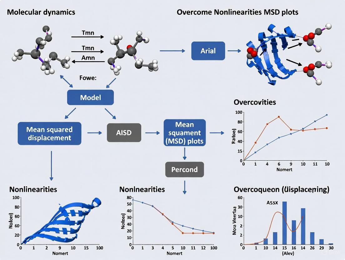
Visualization: Workflow for MSD Analysis

Diagram Title: MSD Analysis and Troubleshooting Workflow

Diagram Title: Common Nonlinear MSD Signatures

---

The Scientist's Toolkit: Research Reagent Solutions

Reagent / Software	Function in Analysis
GROMACS (gmx trjconv)	A core MD simulation suite; its trjconv module is used for trajectory correction (cluster, nojump) and format conversion [1].
VMD	A molecular visualization program for displaying, animating, and analyzing large biomolecular systems. Essential for visually diagnosing trajectory issues [1].
Chimera	A full-featured, Python-based visualization program that can read GROMACS trajectories and is useful for structural analysis [1].
Grace	A WYSIWYG 2D plotting tool, often used to graph data from GROMACS-generated .xvg files, such as MSD plots [1].
Matplotlib	A popular Python library for creating static, animated, and interactive visualizations, commonly used for custom plotting of MSD data [1].
Mal-PEG4-Lys(t-Boc)-NH-m-PEG24	Mal-PEG4-Lys(t-Boc)-NH-m-PEG24, MF:C78H147N5O35, MW:1715.0 g/mol
Montelukast dicyclohexylamine	Montelukast dicyclohexylamine, MF:C47H59ClN2O3S, MW:767.5 g/mol

Frequently Asked Questions (FAQs)

• My MSD plots show clear curvature or plateaus, suggesting heterogeneous motion. What is the first thing I should check? First, verify that your trajectories are sufficiently long. Short trajectories can produce nonlinear MSD plots that are artifacts of limited sampling rather than true heterogeneous diffusion. For reliable characterization of anomalous diffusion, trajectories should span at least two orders of magnitude in time lags [2].

• How can I distinguish between true anomalous diffusion and transient confinement within a single trajectory? Traditional MSD analysis can create ambiguity between a particle's inherent anomalous diffusion and nonlinearity caused by motion constraints [3]. To distinguish them, employ analysis methods that are more sensitive to transient states. The distribution of displacements, angles, or velocities within a trajectory can reveal heterogeneities that are masked in the ensemble-averaged MSD [2]. Hidden Markov Models (HMMs) are also particularly effective for identifying different diffusional states and their switching kinetics [2].

• My single-particle tracking data in a 3D hydrogel is very short and noisy. What analysis methods are robust under these conditions? For short, noisy trajectories, machine learning (ML) classification methods often outperform traditional analyses. ML approaches, from random forest to deep neural networks, can identify motion patterns from predefined or automatically learned features of the trajectory, demonstrating good accuracy even with limited data [2]. Alternatively, active-feedback tracking methods like 3D-SMART can be used to generate the long, highly-sampled trajectories needed for conventional analysis [4].

• Why do my molecular dynamics simulations of a simple diffusive process yield inconsistent results for diffusion coefficients? Classical Molecular Dynamics is a deterministic yet chaotic system. Extreme sensitivity to initial conditions means that even with perfect force fields, one-off simulations are not reproducible in a detailed sense. To obtain reliable and statistically meaningful results, you must use ensemble methods—running a sufficiently large number of replicas with different initial conditions—from which robust average properties and their uncertainties can be extracted [5].

Troubleshooting Guides

Problem 1: Nonlinear or Curved MSD Plots

Symptoms: The Mean Squared Displacement (MSD) plot as a function of time lag (Ï„) is not linear on a log-log scale, showing curvature, plateaus, or other deviations from a straight line.

Potential Causes and Solutions:

Cause	Diagnostic Check	Solution
Short Trajectories	Check trajectory length. MSD curves become unreliable at long time lags (n > N/4) [2].	Use the initial slope of the MSD (first 4-5 points) to estimate a short-term diffusion coefficient. Prioritize obtaining longer trajectories.
True Anomalous Diffusion	Fit MSD with a power law, MSD(τ) ~ τ^α. An exponent α ≠ 1 indicates anomalous diffusion [2].	Use change-point detection algorithms or Hidden Markov Models (HMMs) to segment the trajectory into states with different α or D values [3] [2].
Transient Confinement	Analyze the distribution of step sizes or angles. Confinement often leads to a high frequency of back-and-forth motion [2].	Apply methods like the moment scaling spectrum (MSS) or machine learning classifiers that are sensitive to local motion patterns rather than global averages.
Experimental Noise	Plot the MSD at the shortest time lag. A high y-intercept often indicates significant localization error.	Use analysis frameworks that explicitly account for and correct localization uncertainty in the model [2].

Problem 2: Inconsistent Results from Molecular Dynamics Simulations

Symptoms: Simulations of the same system, but with slightly different initial conditions (e.g., random seed), produce different values for calculated properties like diffusion coefficients or binding free energies.

Potential Causes and Solutions:

Cause	Diagnostic Check	Solution
Chaotic Dynamics	Run 10-20 replicas with different random seeds and calculate the standard deviation of your property of interest. A large variance confirms sensitivity.	Implement a proper ensemble simulation approach. Run a large number of replicas (dozens to hundreds) to build reliable statistics and quantify uncertainty [5].
Insufficient Sampling	Check if the property of interest has converged over the simulation time.	Extend simulation time or use enhanced sampling techniques to overcome energy barriers and sample phase space more effectively [6].
Systematic Force Field Errors	Compare simulated properties with known experimental data.	Re-parameterize or select a more accurate force field. Be aware that different force fields can bias secondary structure formation [5].

Quantitative Data Tables

Table 1: Common Motion Types and Their MSD Characteristics

Motion Type	MSD(τ) Equation	Anomalous Exponent (α)	Typical Physical Scenario
Immobile	Constant	~ 0	Particle tethered or tightly bound.
Brownian (Free Diffusion)	MSD(τ) = 2νDτ	α ≈ 1	Unobstructed random walk in ν dimensions.
Subdiffusion	MSD(τ) = 2νDᵅτᵅ	α < 1	Motion in a crowded or viscoelastic environment [2].
Superdiffusion	MSD(τ) = 2νDᵅτᵅ	α > 1	Active transport with a directional component [2].
Confined	MSD(τ) = L²/3 (1 - A₁exp(-A₂τ/L²))	α → 0 at long τ	Particle trapped in a cage or microdomain [2].

Method Class	Key Principle	Strengths	Limitations
MSD Analysis	Fits mean-squared displacement vs. time lag [2].	Intuitive; well-established fitting models.	Low accuracy for short trajectories; masks heterogeneity.
Change-Point Detection	Identifies points where motion parameters change [3].	Directly segments trajectories; reveals kinetics.	Performance depends on model choice and trajectory length.
Hidden Markov Models (HMM)	Models trajectory as a sequence of hidden states [2].	Infers state populations and transition probabilities.	Requires pre-defining the number of states; can struggle with non-Brownian motion.
Machine Learning (ML)	Classifies motion based on trajectory features [2].	High accuracy for short/noisy tracks; model-free options.	Can be a "black box"; requires training data; computationally intensive.

Experimental Protocols

Protocol 1: Detecting Motion Changes in Single-Particle Trajectories using Change-Point Analysis

This methodology is derived from benchmarks established by the 2nd Anomalous Diffusion (AnDi) Challenge [3].

• Trajectory Acquisition: Obtain single-particle trajectories via live-cell single-molecule imaging and tracking. Ensure a high signal-to-noise ratio and localization precision to minimize artifacts.
• Data Preprocessing: Filter trajectories based on length. For reliable change-point detection, trajectories should ideally contain a minimum of 50-100 steps.
• Algorithm Selection: Choose a change-point detection algorithm designed for single-particle trajectories. The AnDi Challenge provides a performance ranking for various methods [3].
• Parameter Setting: Configure the algorithm's sensitivity (e.g., minimum segment length, significance threshold) based on the expected number of state changes and the signal-to-noise ratio of your data.
• Trajectory Segmentation: Run the algorithm to identify the precise time points (changepoints) where the diffusion coefficient (D) or anomalous exponent (α) changes.
• State Characterization: Analyze each segmented trajectory piece to determine its motion parameters (e.g., D, α, or motion class: confined, Brownian, directed).
• Validation: Validate the identified states and changepoints by comparing the results with other methods, such as HMM or visual inspection of the trajectory and its MSD.

Protocol 2: 3D Single-Molecule Active-feedback Real-time Tracking (3D-SMART) in Porous Materials

This protocol enables the generation of long, high-resolution trajectories necessary to resolve heterogeneous diffusion in complex 3D environments like hydrogels [4].

• Sample Preparation: Fluorescently label nanoparticles of interest. For hydrogel studies, premix nanoparticles into the agarose or other polymer solution before gelation [4].
• Microscope Setup: Use a microscope equipped with 3D active-feedback tracking. The system typically uses electro-optical deflectors (EODs) for lateral scanning and a tunable acoustic gradient (TAG) lens for axial scanning to create a 3D scanning volume of ~1×1×2 μm [4].
• Particle Lock-on: Identify a diffusing nanoparticle and initiate the active-feedback loop. The system uses previous particle position and real-time photon information to estimate the new location.
• Real-Time Tracking: The feedback loop continuously adjusts the position of the scanning volume to "lock" the particle in the center. The voltage signals sent to the EODs and TAG lens are recorded as the particle's 3D trajectory over time.
• Data Collection: Track particles for extended durations (seconds to minutes) to capture rare events like "hopping" between confinement cages [4].
• Trajectory Analysis: Extract quantitative parameters such as confinement sizes, hopping kinetic parameters (on/off rates, lifetimes), and local diffusion coefficients from the highly-sampled trajectories.

Workflow and Relationship Visualizations

The Scientist's Toolkit: Research Reagent Solutions

Table 3: Essential Materials for Single-Particle Tracking Experiments

Item	Function	Example/Notes
Photoactivatable Fluorophores	Enable single-molecule localization by controlling the ON/OFF state of labels in dense environments [7].	Dendra2, mEos3.2, PA-JF dyes. Choice affects photon budget and localization precision.
Self-Labeling Protein Tags	Allow specific labeling of target proteins with bright, photostable organic dyes in live cells [7].	HaloTag, SNAP-tag. Crucial to wash out free dye to reduce background.
Genome Editing Tools	Enable endogenous tagging of proteins, maintaining native expression levels and avoiding artifacts [7].	CRISPR-Cas9. Preferred over overexpression to study true molecular behavior.
3D Active-Feedback Microscope	Generates long, high-spatiotemporal resolution 3D trajectories of rapidly diffusing particles [4].	3D-SMART microscopy. Uses EODs and TAG lens for real-time tracking, overcoming volumetric imaging bottlenecks.
Label-Free Tracking via Caustics	Tracks nanoparticles without fluorescent labels, avoiding phototoxicity and altered physicochemical properties [8].	Uses a standard inverted microscope with enhanced coherence. Ideal for screening in synthetic hydrogels.
(Z)-hexadec-9-en-15-ynoicacid	(Z)-hexadec-9-en-15-ynoicacid, MF:C16H26O2, MW:250.38 g/mol	Chemical Reagent
Fmoc-Phe-Lys(Boc)-PAB-PNP	Fmoc-Phe-Lys(Boc)-PAB-PNP, MF:C49H51N5O11, MW:886.0 g/mol	Chemical Reagent

The Impact of External Fields and Environmental Interactions on Diffusion

Frequently Asked Questions (FAQs)

FAQ 1: Why does my Mean Squared Displacement (MSD) plot show a crossover phenomenon (e.g., from subdiffusive to normal scaling) instead of a straight line?

This is a common observation in compartmentalized or heterogeneous environments, such as within living cells or porous materials. The crossover indicates a transition between two dynamical regimes [9] [10].

• Short-Time Regime: At short timescales, the particle's motion is confined within a local domain or compartment (e.g., a membrane patch or a pore). This confinement often leads to anomalous (non-linear) MSD behavior [10].
• Long-Time Regime: At longer timescales, the particle manages to escape the confinement and hop between domains. This leads to normal, linear MSD scaling (〈x²(t)〉 ~ t), but with a significantly reduced effective diffusion coefficient compared to the local, in-compartment diffusion [10].
• Troubleshooting Tip: This behavior is a hallmark of hop diffusion. Analyze the trajectory for transient confinement zones. The ratio of the short-time to long-time diffusion coefficient provides insight into the molecular properties and barrier permeability of the system [10].

FAQ 2: My MSD increases linearly with time, indicating normal diffusion, but the distribution of particle displacements is non-Gaussian (e.g., shows exponential tails). Why is this happening?

You are observing "Brownian yet non-Gaussian" (BnG) diffusion, a widespread phenomenon in complex environments [9] [10].

• Cause: The BnG diffusion typically arises from population heterogeneity. Your sample may contain a mixture of particles with different diffusion coefficients, or individual particles may be transitioning between different diffusive states over time [11]. The linear MSD suggests normal diffusion on average, but the non-Gaussian displacement distribution reveals the underlying heterogeneity.
• Molecular Origin: In cell membranes, this can be caused by a "quenched disordered environment" where domains or patches with different viscosities or obstacle densities exist stably [9].
• Troubleshooting Tip: Employ analysis methods that are sensitive to multimodal diffusion, such as the logarithmic measure of diffusion [11]. This method transforms displacement data to reveal distinct peaks in the probability density, each corresponding to a different sub-population or diffusive state, without requiring prior labeling.

FAQ 3: How can I distinguish between true anomalous diffusion and transient confinement effects in my molecular dynamics (MD) trajectories?

Disentangling these effects requires analyzing both the MSD and the probability distribution of displacements.

• Genuine Anomalous Diffusion: Manifests as a power-law MSD (〈x²(t)〉 ~ t^β) over a substantial range of time scales, with a constant anomalous exponent β. The displacement distribution may also be non-Gaussian [9].
• Transient Confinement in Compartmentalized Media: Appears as a crossover in the MSD from anomalous to normal diffusion, as described in FAQ 1. The non-Gaussianity in this case is a transient effect. For an ensemble of particles, the displacement distribution at intermediate times is a mixture of the uniform distributions within their respective compartments, which can result in an exponential (Laplace) distribution [10].
• Troubleshooting Tip: Perform a time-dependent analysis of the non-Gaussian parameter α(t) or the displacement distribution. In transient confinement, the non-Gaussianity will peak and then decay as particles begin to explore multiple compartments, whereas in some forms of genuine anomalous diffusion, it may persist.

Troubleshooting Guides

Guide 1: Diagnosing Non-Linear MSD Plots

Symptoms: MSD plot is not a straight line on a log-log scale; it may show a clear crossover or a continuous curvature.

MSD Profile	Potential Cause	Underlying Mechanism	Verification Method
Crossover to Linear MSD	Hop Diffusion / Compartmentalization	Particles are temporarily trapped in domains before hopping to adjacent ones [10].	Check for transient confinement in trajectories; analyze the distribution of waiting times in localized zones.
Persistent Subdiffusion (β < 1)	Crowded Environments / Obstacles	Motion is hindered by a dense network of immobile or slow-moving obstacles, leading to a continuous-time random walk (CTRW) with a heavy-tailed waiting time distribution [9].	Test if the waiting time distribution follows a power law: ω(τ) ~ τ^-(1+σ) [9].
Superdiffusion (β > 1)	Active Transport	Particles are driven by active processes, such as motor proteins, which impart directed motion [11].	Look for directional persistence in trajectories that is not consistent with passive Brownian motion.

Guide 2: Resolving Non-Gaussian Displacement Distributions

Symptoms: A histogram of particle displacements (e.g., over a fixed time lag) does not fit a Gaussian curve; it may have sharp peaks or heavy exponential tails [9] [10].

Observation	Likely Interpretation	Recommended Quantitative Analysis
Exponential (Laplace) Tails	Brownian yet Non-Gaussian (BnG) Diffusion in a static, heterogeneous environment [10].	Apply the logarithmic measure [11]. Calculate the distribution of single-trajectory diffusion coefficients to see if multiple distinct modes exist.
Sharp Peaks with Heavy Tails	May be explained by a CTRW model where the waiting time density has a weak asymptotic property (e.g., power-law) [9].	Analyze the waiting time distribution between significant jumps in the particle's path. Model the data with a coupled CTRW framework [9].

Experimental Protocols & Data Analysis

Protocol 1: Using the Logarithmic Measure to Reveal Multimodal Diffusion

This protocol is ideal for identifying multiple diffusive states from single-particle tracking data without distinct labeling [11].

• Input: A set of 2D particle trajectories {x(t), y(t)}.
• Calculate Increments: For a chosen time lag Δt, compute the displacements for each trajectory: Δr_i = r(t+Δt) - r(t).
• Compute Apparent Diffusion Coefficients: For each displacement vector, calculate an apparent diffusion coefficient D_app using the relation for 2D diffusion: D_app = (Δx² + Δy²) / (4Δt). This generates a large set of D_app values from all trajectories and time points.
• Logarithmic Transform: Create a new dataset of the logarithms of these values: Z = log10(D_app).
• Analyze Distribution: Plot the probability density function (PDF) of Z. Distinct peaks in this PDF correspond to different, coexisting diffusive modes in the sample [11].
• Fit and Interpret: Fit the PDF with a multi-modal model (e.g., a sum of Gaussian distributions) to quantify the number of states, their mean diffusion coefficients, and their relative populations.

Protocol 2: Molecular Dynamics (MD) Simulation of Diffusion in a Compartmentalized System

This protocol outlines how to set up and analyze MD simulations to study the impact of environmental interactions.

• System Setup:
  • Construct a simulation box containing your molecule of interest (e.g., a lipid, drug molecule).
  • Model the compartmentalized environment by introducing barriers or a meshwork of obstacles. These can be represented by fixed, repulsive potential energy grids or explicit immobile atoms [10].
• Simulation Run:
  • Run multiple, long-timescale MD simulations using a suitable force field.
  • Ensure the simulation time is long enough to observe several hopping events between compartments.
• Trajectory Analysis:
  • Calculate MSD: Plot the ensemble-averaged MSD and look for the characteristic crossover from confined to normal diffusion [10].
  • Calculate Non-Gaussian Parameter (NGP): Compute α(t) = 〈Δr⁴(t)〉 / (2 * 〈Δr²(t)〉²) - 1. A significant peak in α(t) confirms transient non-Gaussian dynamics.
  • Displacement Distribution: At a time lag corresponding to the peak of the NGP, plot the histogram of displacements. It should show a strong deviation from a Gaussian, potentially fitting a Laplace distribution [10].

Data Presentation

Table 1: Characteristics of Common Anomalous Diffusion Types

Diffusion Type	MSD Scaling 〈x²(t)〉	Displacement Distribution	Common Physical Cause
Normal (Brownian)	Linear: 2Dt	Gaussian	Unobstructed, homogeneous environment.
Confined / Crossover	Crossover: Anomalous → Linear	Non-Gaussian, often exponential at intermediate times [10]	Transient trapping in compartments (hop diffusion) [10].
Subdiffusive (CTRW)	Power-law: t^β (β<1)	Non-Gaussian	Trapping events with power-law distributed waiting times [9].
Brownian non-Gaussian (BnG)	Linear: 2Dt	Non-Gaussian, exponential tails [9] [10]	Population heterogeneity in a quenched disordered environment [9] [11].

Visualizing Signaling Pathways and Workflows

Troubleshooting Non-Linear MSD

Molecular Interactions in Heterogeneous Environments

The Scientist's Toolkit: Research Reagent Solutions

Item / Reagent	Function in Research	Example Application / Note
Molecular Dynamics (MD) Software	Simulates the physical movements of atoms and molecules over time, allowing for the study of diffusion in bespoke, controlled environments [12] [13].	Used to model hop diffusion in compartmentalized media or to simulate the effect of specific molecular interactions with surfactants or polymers [12].
Continuous-Time Random Walk (CTRW) Model	A mathematical framework used to model anomalous diffusion where waiting times between particle jumps are drawn from a potentially heavy-tailed distribution [9].	Essential for quantifying and interpreting subdiffusion caused by trapping events in crowded environments [9].
Logarithmic Measure Analysis	A data analysis method that transforms displacement data to reveal a spectrum of diffusion coefficients, identifying multiple diffusive modes without distinct labeling [11].	Ideal for analyzing single-particle tracking data from heterogeneous systems like the cell cytoplasm or membrane, where multiple species or states coexist [11].
Lipid Nanoparticles (LNPs)	A delivery system used in drug development, particularly for mRNA vaccines. Their behavior is a practical example of diffusion studies in complex, heterogeneous biomembrane systems [14].	The diffusion of LNPs and their cargo in biological environments is influenced by complex interactions, making them a key area of study [14].
Girard's Reagent P-d5	Girard's Reagent P-d5|Deuterated Stable Isotope	Girard's Reagent P-d5 is a deuterated stable isotope label for precise MS-based quantification of carbonyl compounds like steroids. For Research Use Only. Not for human use.
Omeprazole sulfone-d3	Omeprazole sulfone-d3, MF:C17H19N3O4S, MW:364.4 g/mol	Chemical Reagent

Distinguishing Between Anomalous Diffusion and Experimental Artifacts

## Frequently Asked Questions (FAQs)

Q1: My Mean Squared Displacement (MSD) plot is not linear. Does this always indicate anomalous diffusion? Not necessarily. While a non-linear MSD plot (showing a power-law dependence MSD ∝ t^α with α≠1) can be a signature of anomalous diffusion, it can also be caused by experimental artifacts [15]. Key artifacts to rule out include localization errors (noise), drift in the imaging system, or the presence of physical constraints like confinement that truncate the trajectory [3].

Q2: How can I determine if my short, noisy trajectories show genuine subdiffusion or just measurement error? Traditional MSD analysis breaks down for short or noisy trajectories [15]. It is recommended to use machine-learning-based methods, which were shown in community challenges (the AnDi Challenge) to achieve superior performance in these conditions [15] [3]. These methods are better at characterizing anomalous diffusion from individual trajectories where MSD fitting is unreliable.

Q3: What are the common pitfalls when calculating MSD that could lead to misinterpretation? A major pitfall is using "wrapped" coordinates from simulations with periodic boundary conditions instead of "unwrapped" coordinates, which artificially inflates the MSD [16]. Furthermore, MSD analysis can be ambiguous for heterogeneous or non-ergodic processes, where ensemble and time-averaged MSD are not equivalent [15].

Q4: How can I tell if a change in motion is due to a biological interaction or an artifact? Implementing a rigorous changepoint analysis is key. Methods that segment trajectories to identify points where diffusion properties (like coefficient D or exponent α) change can distinguish true biological transitions (e.g., binding, immobilization) from external drift or other artifacts [3]. The performance of these methods has been benchmarked in the 2nd AnDi Challenge [3].

Q5: My MSD curve has a high error margin. How can I improve the reliability of my diffusion coefficient estimate? For experimental trajectories, use established algorithms that provide error estimates for MSD [17]. Ensure you select a linear segment of the MSD plot for fitting, excluding short time-lags (ballistic motion) and long time-lags (poor averaging) [16]. Combining multiple replicates also improves the accuracy of the averaged MSD [16].

Q6: When should I suspect my instrument is causing apparent anomalous diffusion? Persistent directional motion across multiple, unrelated particles in the field of view often indicates system-wide drift. If the apparent anomalous exponent (α) is not reproducible across different experimental replicates or calibration measurements with particles of known diffusivity show deviations from Brownian motion, an instrumental artifact is likely [3].

## Troubleshooting Guide: Common Symptoms and Solutions

Symptom	Potential Artifact	Underlying Cause	Diagnostic Experiments & Solutions
Apparent subdiffusion (α < 1) at short timescales	Localization noise / measurement error	The inherent uncertainty in pinpointing a particle's position distorts displacement measurements at short time lags [15].	Fit the MSD while accounting for a noise offset [15]. Compare results from machine learning classifiers, which are more robust to noise [15] [3].
MSD curve plateaus or bends at long times	Confinement / finite system size	The particle's motion is physically restricted by boundaries (e.g., cellular organelles, vesicle walls) [3].	Check if the plateau value corresponds to a physical dimension of the system. Use models designed for confined diffusion instead of free diffusion.
Superdiffusion (α > 1) in a static sample	Stage or fluid drift	The entire sample is moving slowly in one direction, adding a directed component to random particle motion [3].	Track immobilized particles or fiducial markers to quantify and subtract drift. Ensure the microscope stage and sample are thermally stabilized.
High variability in α between trajectories	Mixture of particle populations or states	Genuine biological heterogeneity, where particles exist in different functional states (e.g., bound vs. unbound) [3].	Perform changepoint analysis to segment trajectories before calculating α [3]. Use statistical tests to confirm the presence of multiple populations.
MSD is linear but the diffusion coefficient seems too low	Viscosity mismatch or crowding	The solution viscosity is higher than assumed, or the environment is densely crowded, slowing diffusion.	Measure the diffusivity of standard particles in the same buffer. Account for the effects of macromolecular crowding in your model.

## Quantitative Data for Anomalous Diffusion Analysis

Table 1: Key Properties of Common Anomalous Diffusion Models. This table helps identify the underlying model based on trajectory properties [15] [3].

Model Name	Key Mechanism	MSD Scaling (α)	Ergodicity	Increment Distribution
Fractional Brownian Motion (FBM)	Long-range correlated noise [3]	α = 2H (H is Hurst exponent)	Ergodic	Gaussian
Continuous-Time Random Walk (CTRW)	Power-law distributed waiting times between steps [15]	α < 1	Non-ergodic	Can be non-Gaussian
Lévy Walk	Power-law distributed step lengths [15]	1 < α < 2 (superdiffusion)	Non-ergodic	Heavy-tailed
Scaled Brownian Motion (SBM)	Time-dependent diffusion coefficient D(t) [15]	α ≠ 1	Ergodic	Gaussian
Annealed Transient Time Motion (ATTM)	Diffusivity that changes over time in a stochastic manner [15]	α < 1	Non-ergodic	Can be non-Gaussian

Table 2: MSD-Based Diagnostics for Common Artifacts. This table summarizes how artifacts manifest in MSD analysis.

Artifact Type	Effect on MSD Plot	Effect on Anomalous Exponent α	How to Mitigate
Localization Noise	Upward curvature at the shortest time lags; MSD does not approach zero at Δt→0 [15].	Biases estimates of α downwards, creating false subdiffusion.	Incorporate a noise term in the MSD fitting model: MSD(Δt) = 4D(Δt)^α + 2σ², where σ is localization precision [15].
Constant Drift	MSD grows quadratically (∝ Δt²) at long times, mimicking ballistic motion [3].	Biases α towards 2.	Track fiducial markers or immobilized particles to measure and subtract the drift vector from each frame [3].
Confinement	MSD plateaus to a constant value at long time lags [3].	The effective α approaches 0 at long times, regardless of the initial motion.	Use a confined diffusion model for fitting. Focus analysis on the initial, linear part of the MSD before the plateau.

## Experimental Protocols

Protocol 1: Proper Calculation of MSD from Trajectories

Objective: To accurately compute the MSD from a particle trajectory while avoiding common computational errors [16].

• Input: Use particle trajectories with unwrapped coordinates. If your data comes from simulations with periodic boundary conditions, ensure particles are not artificially wrapped back into the primary cell [16].
• Calculation: Apply the Einstein formula using an efficient algorithm. For a trajectory with positions ( r(t) ), the MSD for a lag time ( \tau ) is: ( \text{MSD}(\tau) = \langle | r(t + \tau) - r(t) |^2 \rangle ), where ( \langle \cdot \rangle ) denotes averaging over all time origins t [16].
• Efficiency: For long trajectories, use a Fast Fourier Transform (FFT)-based algorithm to reduce computational complexity from O(N²) to O(N log N) [16].
• Combining Replicates: When multiple trajectories are available, average the MSDs from each particle. Do not simply concatenate trajectories, as the jump at the concatenation point will artificially inflate the MSD [16].

Protocol 2: Differentiating Anomalous Diffusion from Heterogeneity via Changepoint Analysis

Objective: To determine if a trajectory stems from a single anomalous diffusion model or from a particle switching between different dynamic states [3].

• Data Simulation for Benchmarking: Generate ground-truth trajectories using fractional Brownian motion (FBM) with piecewise-constant parameters (D or α). This simulates a particle changing its motion, e.g., upon binding [3].
• Method Selection: Choose a segmentation method benchmarked in the 2nd AnDi Challenge. These are designed to identify the precise points (changepoints) where diffusion properties change [3].
• Trajectory Segmentation: Apply the chosen algorithm to your experimental trajectory. The output will be a series of segments, each with its own estimated parameters.
• Validation: Calculate the MSD and/or other properties for each segmented state independently. A successful analysis will show a linear MSD on a log-log plot for each segment, confirming a well-defined state, and will resolve the heterogeneity that caused the original, non-linear MSD.

## Workflow and Pathway Visualizations

Diagram 1: Decision Tree for Anomalous Diffusion Analysis

This workflow provides a step-by-step guide to diagnose the source of non-Brownian motion in your data.

Diagram 2: MSD Calculation and Fitting Workflow

This diagram outlines the correct procedure for calculating MSD and extracting a diffusion coefficient, highlighting key troubleshooting points.

## The Scientist's Toolkit: Essential Reagents and Software

Table 3: Key Research Reagent Solutions for Anomalous Diffusion Studies.

Item Name	Function / Role	Example Use Case
Fiducial Markers (e.g., fluorescent beads)	Provides a fixed reference point to detect and correct for system-wide drift during imaging [3].	Immobilized on the coverslip near the sample to track and subtract stage drift from particle trajectories.
Standard Calibration Particles	Particles with known, stable diffusion coefficient (D) in a given buffer.	Used to validate microscope setup and MSD analysis pipeline, ensuring measured D matches expected values.
andii-datasets Python Package	A software library to generate simulated trajectories with known ground truth for benchmarking analysis methods [3].	Simulating fractional Brownian motion (FBM) trajectories to test the performance of a new changepoint detection algorithm.
KMCLib Software	A program for kinetic Monte Carlo (KMC) simulations, which can model diffusion processes with non-equidistant time-steps [17].	Studying atomic-scale diffusion events that are too slow for molecular dynamics, including MSD calculation with error estimates.
MDAnalysis Python Package	A toolkit to analyze molecular dynamics trajectories, including standardized MSD calculation [16].	Analyzing simulated MD trajectories of a protein in solution to compute its self-diffusivity from the MSD.
1,3-Dipalmitoyl-2-linoleoylglycerol	1,3-Dipalmitoyl-2-linoleoylglycerol, MF:C53H98O6, MW:831.3 g/mol	Chemical Reagent
11-O-Methylpseurotin A	11-O-Methylpseurotin A, MF:C22H25NO8, MW:431.4 g/mol	Chemical Reagent

How Polymer Chain Dynamics and Confinement Create Non-Linear MSD Profiles

Troubleshooting Guide: Resolving Non-Linear MSD Profiles

Problem Area	Specific Issue	Potential Causes	Recommended Solutions
System & Confinement	Sub-diffusive or flattened MSD at intermediate times	Chain motion restricted by topological constraints or geometrical confinement [18]	- Characterize confinement geometry (e.g., pore size, NP spacing) [19].- Analyze chain conformation (e.g., Rg) vs. confinement size [19].
	Dynamical heterogeneity, multiple relaxation regimes	Presence of both "dry"/slow and "wet"/fast chain regions [18]	- Use site-specific labeling (e.g., inner vs. outer chain segments) [18].- Employ models with site-dependent friction [18].
Entanglements & Topology	Crossover to sub-diffusive behavior, reptation dynamics	Onset of entanglement effects; chain motion confined to a tube [20] [21]	- Verify simulation/model against active reptation theory predictions [21].- Calculate entanglement length (Me) for your system [22].
Simulation & Analysis	Numerical instability at high fields or long times	Extreme electric fields lowering effective barriers unrealistically [23]	- Check field strength stability (e.g., < 0.1 V/nm for PEO/LiTFSI) [23].- Use appropriate thermostats (e.g., Nose-Hoover) [22].
	MSD artifacts from poor equilibration	Insufficient relaxation of initial configuration, especially for dense/glassy systems [22]	- Perform long NPT runs to equilibrate density [22].- Check energy and pressure stability before production run.
Polymer-Specific Interactions	Segmental dynamics slower than expected	Increased monomeric friction near surfaces/grafting points [18]	- Incorporate friction profiles in analysis models [18].- Check for specific polymer-surface interactions (e.g., γSL) [19].

Frequently Asked Questions (FAQs)

Q1: My MSD plot for a confined polymer system shows a clear plateau or severely suppressed dynamics. What does this mean?

This is a classic sign of confinement-induced dynamical heterogeneity. Your system likely contains chain segments with drastically different mobilities. For instance, in polymer-grafted nanoparticles, segments near the grafting point ("dry layer") experience much higher friction and slower dynamics than segments in the outer regions ("wet layer") [18]. This creates an average MSD that appears flattened.

• How to verify: Use a technique like Neutron Spin Echo (NSE) with selective deuterium labeling on different parts of the chain (inner vs. outer segments). This allows you to probe the dynamics of specific chain sections rather than the global average [18].
• How to model: Avoid models that assume a single, homogeneously relaxing ensemble. Instead, use an analysis that allows for at least two differently relaxing chain ensembles or a position-dependent friction coefficient [18].

Q2: In my simulations of entangled polymers, the MSD shows a distinct sub-diffusive regime (∼t^0.5). What is the physical origin of this, and how can I validate my model?

The sub-diffusive regime where MSD ∝ t^0.5 is the signature of reptation dynamics. The chain is confined to a tube created by the topological constraints of its neighboring chains, and its motion is primarily one-dimensional diffusion along the tube contour [20] [21].

• How to validate: A powerful method is to simulate active entangled polymers. Apply a constant force that imparts a drift velocity along the primitive path of the chain. A valid model will show that while conformational properties (e.g., Rg) remain largely unchanged, the dynamics are strongly accelerated, and the diffusion coefficient becomes independent of molecular weight at moderate activity levels, as predicted by active reptation theory [21].

Q3: When applying an electric field in my ion-conducting polymer simulations, the MSD/conductivity becomes highly non-linear and the simulation becomes unstable. What should I check?

This indicates you are in the high-field non-linear regime. The electric field is tilting the energy landscape, reducing the effective barriers for ion hopping, and can eventually cause numerical instabilities [23].

• How to diagnose:
  • Check field strength: Compare your field (E) to known thresholds. For a PEO/LiTFSI electrolyte, strong non-linear effects appear above ~0.1 V/nm, and simulations can become unstable at higher fields [23].
  • Analyze hopping distances: In the high-field regime, you can extract an effective hopping distance. This value should be comparable to typical ion-ion or ion-polymer coordination distances (on the order of Ã…ngströms) from your system's structural analysis [23].
• How to proceed: Ensure you are using a robust thermostat and consider using a smaller timestep or a different integration algorithm for high-field simulations.

Experimental & Simulation Protocols

Protocol 1: Probing Confined Dynamics with Neutron Spin Echo (NSE) Spectroscopy

This protocol is based on studies of one-component nanocomposites (OCNCs) where polymers are grafted to nanoparticle cores [18].

• Sample Synthesis:
  • System: Create block-copolymers with a cross-linked core (e.g., deuterated 1,2-polybutadiene) and a grafted shell (e.g., poly(ethylene oxide), PEO) [18].
  • Labeling: Prepare at least three differently labeled versions:
    • Inner-labeled: Tags attached near the grafting point to the nanoparticle.
    • Outer-labeled: Tags attached to the free ends of the grafts.
    • Fully-labeled: The entire graft is labeled [18].
• Structural Characterization:
  • Use Small-Angle X-Ray/Neutron Scattering (SAXS/SANS) to determine the nanoparticle structure, size distribution, and overall melt structure. A Percus-Yevick structure factor can model a concentrated colloidal dispersion [18].
• Dynamic Measurement:
  • Perform Neutron Spin Echo (NSE) Spectroscopy on all labeled samples.
  • NSE measures the intermediate scattering function, providing direct insight into the segmental and chain dynamics on nanosecond to hundred-nanosecond timescales [18].
• Data Analysis:
  • Do not fit the data with a single phenomenological function (e.g., KWW) for the entire chain.
  • Solve a Langevin equation that includes a spatial friction profile.
  • Compare the calculated dynamic structure factor (using its eigenvalues and eigenvectors) to the experimental data. This will reveal the increased friction towards the grafting points and the effect of topological restrictions [18].

Protocol 2: Simulating Active Entangled Polymer Dynamics

This protocol outlines how to use molecular dynamics (MD) to verify entanglement dynamics and understand the MSD, based on the work of [21].

• System Setup:
  • Model: Use a coarse-grained model like the Kremer-Grest bead-spring model.
  • System Composition: Simulate a few active, shorter chains diluted in a mesh of very long, passive linear chains. This setup minimizes "constraint release" effects from the motion of the surrounding matrix [21].
• Simulation Execution:
  • Apply a constant active force of the form Factive = Fa * u. Here, u is the unit vector along the end-to-end direction of the chain, imparting a polar drift velocity along the chain's primitive path [21].
  • Run simulations for a wide range of activity values (F_a).
• Data Analysis and Validation:
  • Conformational Properties: Confirm that the radius of gyration (Rg^2) and tube structure are not significantly altered by the activity.
  • Dynamics: Calculate the MSD and chain diffusion coefficient.
  • Validation Check: Verify that your results match key predictions of active reptation theory:
    • The chain diffusion coefficient becomes independent of molecular weight at moderate activity levels.
    • A significant reduction in viscosity is observed due to accelerated relaxation [21].

Diagram Title: Diagnostic Workflow for Non-Linear MSD Profiles

The Scientist's Toolkit: Key Research Reagents & Materials

Item	Function & Role in Analysis
Selective Deuterium Labeling	Enables probing site-specific dynamics in NSE experiments. Labels on inner/outer chain segments reveal heterogeneous friction and mobility [18].
One-Component Nanocomposites (OCNCs)	Model system for studying chain confinement. Self-assembled particles with grafted polymers provide a well-defined, dispersed nanostructure without aggregation issues [18].
Coarse-Grained MD Models (e.g., Kremer-Grest)	Computational tool for simulating long-time chain dynamics. Allows control over parameters like entanglement length and application of active forces to test theories [21].
Anodic Aluminum Oxide (AAO) Membranes	A versatile mesoporous template with tunable pore size for experimental studies of polymers under strict geometrical confinement [19].
Poly(ethylene oxide) (PEO)	A widely used model polymer in both simulations and experiments for studying dynamics, ion conduction, and mechanical properties [22] [23].
(S,R,S)-AHPC-Me-C10-NH2	(S,R,S)-AHPC-Me-C10-NH2, MF:C34H53N5O4S, MW:627.9 g/mol
Boc-Aminooxy-PEG5-amine	Boc-Aminooxy-PEG5-amine, MF:C17H36N2O8, MW:396.5 g/mol

Advanced Analytical Frameworks: From Theory to Practical Implementation

Implementing Robust Changepoint Detection for Trajectory Segmentation

Frequently Asked Questions (FAQs)

FAQ 1: What is change-point detection (CPD) and why is it important for analyzing molecular dynamics trajectories? Change-point detection (CPD) is the problem of identifying abrupt variations or changes in the distribution of a temporal signal [24]. In molecular dynamics (MD), this helps pinpoint precise moments of structural transitions—such as nucleation events, protein folding, or phase changes—within a particle trajectory [25]. Automating this detection is crucial for large-scale studies where manual inspection of hundreds of simulations is infeasible. It enables accurate segmentation of trajectories into stable meta-stable states and transition regions, which is foundational for calculating meaningful physical properties like diffusivity from segments of the Mean Squared Displacement (MSD) plot that exhibit linear behavior [26].

FAQ 2: My MSD plot is nonlinear. How can changepoint detection help? A nonlinear MSD plot often indicates that a single diffusion mode does not describe the entire trajectory. The system may undergo a transition between different states (e.g., from ballistic to diffusive motion, or between confined and free diffusion). Robust changepoint detection can automatically segment the full trajectory into homogeneous intervals, each potentially corresponding to a distinct dynamical state [25] [24]. You can then compute an MSD for each segment, which should yield a linear relationship for the middle section of the MSD plot, allowing for an accurate calculation of the self-diffusivity, D, using the Einstein relation: (D_d = \frac{1}{2d} \times \text{slope of the MSD}) [26].

FAQ 3: What is the difference between offline and online changepoint detection? The choice between offline and online algorithms depends on your experimental needs [24].

Feature	Offline Detection	Online Detection
Data Access	Processes the complete dataset simultaneously [24]	Processes data points sequentially as they arrive [24]
Primary Use	Post-analysis, for accurate identification of all changes [25]	Real-time monitoring, for immediate response to changes [25]
Example in MD	Analyzing a completed simulation to find all folding events [25]	Triggering high-frequency data storage upon a nucleation event [25]

FAQ 4: What are some common cost functions for CPD, and how do I choose? Cost functions measure the homogeneity of data within a segment. Two common types are:

• Piecewise Linear Fit: Implemented in tools like dupin, these cost functions are sensitive to shifts in the mean or trend of a signal [25]. They are generally effective for detecting changes in the baseline of order parameters or MSD-derived signals.
• Robust/Wilcoxon-Type: Based on ranks or spatial signs rather than raw values, these functions are less sensitive to outliers in the data [27]. They are advantageous when your trajectory or derived signal contains substantial noise or extreme values.

For molecular trajectories, start with a piecewise linear model. If you suspect your data contains outliers that are causing false positives, switch to a robust method [27].

Troubleshooting Guides

Issue 1: The detector fails to find the correct changepoints.

Potential Cause and Solution Tree:

Detailed Solutions:

• Poor Descriptor Selection: The chosen descriptor must be sensitive to the structural or dynamic transition you want to detect [25].

  • Actionable Protocol: Compute a diverse set of order parameters for your system. For local structural changes (e.g., crystallization), use Steinhardt order parameters or Smooth Overlap of Atomic Positions (SOAP). For dynamical transitions visible in the MSD, ensure you are using unwrapped coordinates to compute the MSD [26]. Using a combination of descriptors often yields the best results.

• Incorrectly Tuned Detection Sensitivity: All CPD algorithms have parameters that control how sensitive they are to changes.

  • Actionable Protocol: Most cost-based methods require a penalty parameter that prevents over-segmentation. Use the "elbow" method on the cost function to determine the correct number of changepoints [25]. Manually annotate a small portion of your trajectory to validate the algorithm's performance and tune the parameters accordingly.

• Underlying Signal is Too Noisy:

  • Actionable Protocol: Apply a smoothing filter (e.g., a Savitzky-Golay filter) to your generated signal before running the CPD algorithm. Alternatively, use a robust changepoint detection method that is less sensitive to outliers, such as one based on U-statistics or spatial signs [27].

Issue 2: Implementing online detection for real-time analysis.

Potential Cause and Solution Tree:

Detailed Solutions:

• Handling Data Streams:

  • Actionable Protocol: Implement an ε-real-time algorithm [24]. This means the algorithm processes data in small, sequential batches of size ε (e.g., every 10-100 simulation frames). Tools like dupin are designed with interfaces suitable for such online detection, allowing you to update the detection model as new data arrives [25].

• Minimizing Detection Lag:

  • Actionable Protocol: The choice of ε is a trade-off. A smaller ε (e.g., 1) provides the fastest response but might be less statistically reliable. A larger ε provides more data points for a confident decision but introduces a longer lag. Optimize this for your specific application by testing different batch sizes on a pre-recorded trajectory.

Experimental Protocols & Data

Protocol 1: Generating a Signal for Trajectory Segmentation from MSD

• Unwrap Coordinates: Ensure your particle trajectory is in unwrapped coordinates to prevent artificial jumps from periodic boundary conditions from skewing the MSD calculation [26].
• Calculate MSD: For a given particle or group of particles, compute the MSD over the entire trajectory using the Einstein formula. Efficient FFT-based algorithms (e.g., in MDAnalysis.analysis.msd with fft=True) are recommended for long trajectories [26].
• Preprocess the MSD Signal: The raw MSD plot is often noisy. Apply smoothing and then compute the instantaneous slope (e.g., by numerical differentiation) or use the MSD values directly as the input signal for CPD. The choice depends on whether you are interested in changes in the mean value or the trend of the MSD.
• Apply Changepoint Detection: Feed the preprocessed signal into your chosen CPD algorithm (e.g., dupin with a piecewise linear cost function) to identify points where the diffusion characteristics change [25].

Protocol 2: Validating Detected Changepoints

• Manual Annotation: Create a "ground truth" by manually identifying obvious transition points in a small subset of your trajectories.
• Compute Metrics: Compare the algorithm's output to your ground truth. Standard metrics include:
  • Precision: The percentage of detected changepoints that are correct.
  • Recall: The percentage of actual changepoints that were successfully detected.
  • Time Lag: For online detection, the average delay between a true change and its detection.
• Cross-Validation: Use the parameters that work best on your validation set for the full analysis.

Comparison of CPD Algorithms

The table below summarizes different CPD approaches relevant to MD analysis.

Algorithm / Tool	Core Methodology	Key Strength	Potential Limitation
dupin [25]	Cost-based optimization with piecewise linear models; interfaces with ruptures library.	Highly automated pipeline; applicable to both offline and online detection.	Performance heavily relies on selection of informative input descriptors.
BEAST [28]	Bayesian ensemble modeling to average multiple decomposition models.	Provides credible uncertainty measures (e.g., probability of changepoints).	Computationally intensive, may be slow for very long trajectories.
Robust CUSUM [27]	Based on U-statistics and spatial signs (generalized Wilcoxon test).	Less sensitive to outliers in the data compared to classical CUSUM.	More complex implementation; may require custom bootstrap for critical values.
Classical CUSUM	Cumulated sums of deviations from the mean.	Simple and computationally efficient.	Sensitive to outliers and assumes a specific change type (e.g., mean shift).

The Scientist's Toolkit: Research Reagent Solutions

Tool / Resource	Function in Experiment	Relevant Context
dupin [25]	A Python package for automatic event detection in particle trajectories. It performs data preprocessing, augmentation, and CPD.	The primary tool for segmenting trajectories based on changes in order parameters or other signals.
MDAnalysis [26]	A Python toolkit to analyze MD trajectories. Its EinsteinMSD module is used to compute MSDs.	Used in the preprocessing stage to convert particle positions into an MSD signal for CPD.
freud [25]	A Python library for efficient analysis of particle trajectories and calculation of order parameters.	Used to compute descriptors like Steinhardt order parameters, which serve as the input signal for dupin.
Ruptures [25]	A Python library for offline changepoint detection with multiple cost functions and search methods.	Can be used as the core detection algorithm within a larger pipeline, either directly or via dupin.
HOOMD-blue [25]	A general-purpose particle simulation toolkit used to generate the MD trajectories.	The source of the raw trajectory data that needs to be segmented and analyzed.
signac [25]	A Python framework for managing and organizing large-scale simulation data and workflows.	Helps manage the data from hundreds of simulations, making CPD workflows reproducible and scalable.
Boc-PEG4-sulfone-PEG4-Boc	Boc-PEG4-sulfone-PEG4-Boc, MF:C30H58O14S, MW:674.8 g/mol	Chemical Reagent
Propargyl-PEG3-methyl ester	Propargyl-PEG3-methyl ester, CAS:2086689-09-8, MF:C11H18O5, MW:230.26 g/mol	Chemical Reagent

Leveraging Machine Learning for Automated MSD Analysis and Pattern Recognition

Frequently Asked Questions (FAQs)

Q1: Why does my MSD plot show a plateau or decreased slope at longer lag times instead of a linear relationship? This indicates insufficient sampling or trajectory length. The MSD requires adequate sampling for accurate diffusion calculation. If your trajectory is too short, the MSD at longer lag times becomes noisy and poorly averaged [29]. Solution: Increase simulation time or use the -maxtau flag in GROMACS to cap maximum time delta and avoid miscalculations from undersampled regions [30].

Q2: My MSD analysis shows anomalously high values. What could be causing this? This often results from using wrapped instead of unwrapped coordinates. When atoms cross periodic boundaries and are wrapped back into the primary cell, it artificially inflates displacement measurements [29]. Solution: Always use unwrapped trajectories. In GROMACS, use gmx trjconv -pbc nojump; in MDAnalysis, ensure coordinates follow the unwrapped convention before MSD calculation [29].

Q3: How can I determine the optimal linear segment for diffusion coefficient calculation? The linear segment represents the "middle" of the MSD plot, excluding ballistic trajectories at short time-lags and poorly averaged data at long time-lags [29]. Solution: Create a log-log plot where the linear segment shows a slope of 1. Use -beginfit and -endfit parameters in GROMACS or manually select the range as demonstrated in MDAnalysis documentation [30] [29].

Q4: What does poor contrast ratio in my MSD visualization indicate, and why does it matter? While not affecting computational results, poor contrast (below 4.5:1 for standard text) hinders interpretation and publication quality [31] [32]. Solution: Ensure foreground-background color pairs meet WCAG guidelines. For molecular visualization, use high-contrast color palettes with minimum 3:1 ratio [31].

Q5: My MSD calculation is extremely slow with long trajectories. How can I optimize performance? The standard MSD algorithm has O(N²) scaling with trajectory length [29]. Solution: Use FFT-based algorithms (set fft=True in MDAnalysis or similar implementations) which reduce scaling to O(N log N). In GROMACS, use -maxtau to limit maximum time delta [30] [29].

Troubleshooting Guides

Issue: Nonlinear MSD Plots in Molecular Dynamics

Problem Identification Nonlinear MSD plots deviate from the theoretical linear relationship expected for normal diffusion, showing curved segments that complicate diffusion coefficient calculation.

Root Causes

• Insufficient sampling at long lag times [29]
• Finite size effects from simulation box constraints [29]
• Anomalous diffusion processes in complex molecular systems [33]
• Coordinate wrapping artifacts from periodic boundary conditions [29]
• Non-equilibrium dynamics during simulation timeframe [33]

Step-by-Step Resolution

• Validate trajectory preprocessing: Ensure proper unwrapping of coordinates using gmx trjconv -pbc nojump (GROMACS) or equivalent in other packages [29].
• Assess sampling adequacy: Plot MSD with error estimates using NBlocksToCompare option in trajectory analysis tools [34].
• Identify linear regime: Generate log-log plot to identify segment with slope ≈1 indicating normal diffusion [29].
• Apply appropriate fitting: Use only the linear segment for diffusion calculation with -beginfit and -endfit parameters [30].
• Implement machine learning detection: Train pattern recognition models to automatically identify linear regions using feature vectors derived from MSD curvature [33].

Prevention Strategies

• Ensure trajectory lengths exceed diffusion timescales by 10-100x [29]
• Use multiple replicates combined with ensemble averaging [29]
• Implement automated quality checks with ML-based pattern recognition [33] [35]

Issue: Memory Errors During Large-Scale MSD Analysis

Problem Identification MSD calculations fail due to insufficient memory, particularly with long trajectories or large molecular systems.

Technical Background Standard MSD algorithm memory requirements scale with O(τmax²) where τmax is maximum lag time [30] [29].

Resolution Protocol

• Implement FFT-based algorithms: Use fft=True in MDAnalysis or equivalent FFT implementations [29].
• Limit maximum lag time: Apply -maxtau parameter in GROMACS to cap time delta [30].
• Strategic frame sampling: Use -dt option to analyze subsets of frames [30].
• Distributed computing: Split analysis across multiple replicates or system partitions [29].
• Progressive analysis: Use -trestart to control restarting point frequency [30].

Table 1: MSD Algorithm Performance Characteristics

Algorithm	Time Complexity	Memory Usage	Implementation
Standard Windowed	O(N²)	High	GROMACS gmx msd
FFT-Based	O(N log N)	Moderate	MDAnalysis fft=True
Block Averaging	O(N)	Low	AMS NBlocksToCompare

Issue: Inconsistent Diffusion Coefficients Across Replicates

Problem Identification Significant variation in calculated diffusion coefficients between simulation replicates under identical conditions.

Diagnostic Procedure

• Calculate inter-replicate variance: Use NBlocksToCompare functionality to obtain error estimates [34].
• Check equilibration: Ensure all replicates reached proper equilibrium before MSD analysis.
• Verify consistent preprocessing: Confirm identical unwrapping and alignment protocols [29].
• Assess statistical convergence: Determine if sampling adequately captures diffusion timescale.

Resolution Framework

• Combine replicates properly: Use appropriate concatenation methods that avoid artificial inflation between trajectories [29].
• Implement ensemble averaging: Calculate average MSD across multiple replicates rather than averaging diffusion coefficients.
• Apply block analysis: Divide individual trajectories into blocks for error estimation [34].
• Utilize ML pattern recognition: Train models to identify systematic errors across replicates [33] [36].

Experimental Protocols

Protocol 1: Standardized MSD Analysis with Linear Regression

Objective: Calculate diffusion coefficient from molecular dynamics trajectory with proper error estimation.

Materials and Software

• Molecular dynamics trajectory (unwrapped coordinates)
• GROMACS, MDAnalysis, or AMS analysis suite
• Python/NumPy/SciPy for additional analysis

Step-by-Step Procedure

• Trajectory Preparation: Convert to unwrapped coordinates using gmx trjconv -pbc nojump or equivalent [29].
• MSD Calculation: Execute MSD analysis with appropriate parameters:
  [30]
• Linear Segment Identification: Plot MSD with log-log scale and identify region with slope ≈1 [29].
• Diffusion Coefficient Calculation: Apply linear regression to selected segment:
  [29]
• Error Estimation: Calculate standard error from regression or block analysis [34].

Quality Control Metrics

• Regression R² value > 0.98 for linear segment
• Adequate sampling indicated by smooth MSD curve in fitting region
• Multiple replicate consistency within statistical error

Protocol 2: Machine Learning-Enhanced MSD Analysis

Objective: Implement pattern recognition to automatically identify linear MSD regions and classify diffusion behavior.

Feature Engineering

• Curvature Features: Calculate second derivative of MSD across multiple window sizes [33].
• Statistical Moments: Compute skewness and kurtosis of MSD slope distribution [33].
• Time-Scale Features: Extract characteristic timescales from MSD curvature transitions [33] [36].
• Noise Metrics: Quantify signal-to-noise ratio at different lag times [33].

Model Training Protocol

• Dataset Preparation: Curate labeled MSD trajectories with expert-identified linear regions [36].
• Feature Extraction: Compute comprehensive feature vectors for each MSD profile [33].
• Model Selection: Train multiple architectures (logistic regression, neural networks) for linear region classification [35] [36].
• Validation: Test model performance against held-out expert annotations [36].

Implementation

Experimental Workflows

MSD Analysis and Troubleshooting Workflow

The Scientist's Toolkit

Table 2: Essential Research Reagents and Software Solutions

Tool/Reagent	Function/Purpose	Implementation Example
Trajectory Unwrapping Tools	Corrects periodic boundary artifacts in coordinates	GROMACS gmx trjconv -pbc nojump [29]
FFT-MSD Algorithms	Enables efficient MSD calculation for long trajectories	MDAnalysis EinsteinMSD with fft=True [29]
Block Analysis Framework	Provides error estimation through trajectory segmentation	AMS NBlocksToCompare parameter [34]
Linear Regression Modules	Calculates diffusion coefficients from MSD slopes	SciPy linregress with optimized fitting range [29]
Pattern Recognition Models	Automates identification of linear MSD regions	ML classifiers trained on MSD curvature features [33] [36]
Contrast Verification Tools	Ensures visualization accessibility for publications	WCAG contrast checkers (minimum 4.5:1 ratio) [31] [32]
N-(Mal-PEG6)-N-bis(PEG7-TCO)	N-(Mal-PEG6)-N-bis(PEG7-TCO), MF:C78H137N7O30, MW:1652.9 g/mol	Chemical Reagent
4-(6-Methyl-1,2,4,5-tetrazin-3-yl)phenol	4-(6-Methyl-1,2,4,5-tetrazin-3-yl)phenol|Tetrazine Linker	4-(6-Methyl-1,2,4,5-tetrazin-3-yl)phenol is a methyltetrazine linker with a phenol group for bioconjugation research. This product is For Research Use Only. Not for human use.

ML Pattern Recognition for MSD Analysis

Frequently Asked Questions

• What is the fundamental theory behind calculating self-diffusivity from MSD? The self-diffusion coefficient (D) is calculated from the mean square displacement (MSD) using the Einstein relation. In three dimensions, the formula is: [ D = \frac{1}{6} \lim_{t \to \infty} \frac{d}{dt} \text{MSD}(t) ] In practice, D is determined by calculating one-sixth of the slope of the MSD versus time plot in the linear regime [37] [38]. The GROMACS gmx msd tool performs a least-squares fitting of a straight line (D*t + c) to the MSD curve to provide the diffusion constant [39].

• Which GROMACS tool is used for MSD calculation and what is its basic syntax? The gmx msd tool is used to compute mean square displacements. A basic command syntax is:

  This command will calculate the MSD for all atoms in the trajectory against the structure file and output the results to an .xvg file [39].

• Why is my MSD plot non-linear or wobbly, and how can I fix it? Non-linear or noisy MSD plots, especially at long time scales, are often a sign of poor sampling. This can manifest as a wobbly line after an initial straighter region [39]. To mitigate this:

  • Ensure your production simulation is long enough; the linear regime of the MSD must be sufficiently sampled.
  • Use the -maxtau option to cap the maximum time delta for frame comparison, which can avoid poorly averaged data at long time lags [39].
  • For individual molecules, use the -mol option, which can provide a more accurate error estimate based on statistics between molecules [39].

• I get an error about 'non-integral time'. What does this mean and how do I resolve it? This error occurs when the gmx msd tool encounters non-integer time values in your trajectory, which disrupts its internal time discretization. The solution is to subsample your trajectory to ensure time steps are integers. You can use the gmx convert-trj tool for this purpose [40]:

  Then, use the new prod_subsampled.xtc file for your MSD analysis.

• Why is it critical to use 'unwrapped' coordinates for a correct MSD calculation? Using wrapped coordinates (where molecules are put back into the primary simulation cell when they cross the periodic boundary) will cause the MSD to be artificially low and eventually plateau. The MSD calculation requires unwrapped coordinates that accurately reflect the true distance a particle has traveled. In GROMACS, you can ensure this by using the -pbc nojump flag with gmx trjconv to remove periodic boundary effects before analysis [16].

• What are the key parameters in gmx msd that control the linear fit for the diffusion coefficient? The most critical parameters for defining the linear region of the MSD plot for diffusion coefficient calculation are -beginfit and -endfit. These specify the time range for the linear regression.

  • By default, if -beginfit is set to -1, the fitting starts at 10% of the total time.
  • If -endfit is set to -1, the fitting goes to 90% of the total time [39]. You should visually inspect your MSD plot to identify the linear regime and set these parameters accordingly.

• My gmx msd analysis is slow or runs out of memory. How can I improve performance? The MSD calculation can be computationally intensive and scale poorly with trajectory length. To improve performance and avoid out-of-memory errors:

  • Use the -maxtau option to limit the maximum time delta for frame comparisons, reducing both computation time and memory usage [39].
  • Analyze a smaller, representative group of atoms or molecules.
  • Consider using a trajectory with a lower time resolution (e.g., by using gmx convert-trj -dt to save frames less frequently).

• How do I calculate the MSD for the center of mass of molecules, rather than individual atoms? Use the -mol flag. This option will make molecules whole across periodic boundaries and plot the MSD for the center of mass of individual molecules. When using -mol, the chosen index group will be automatically split into molecules [39].

Troubleshooting Guide

This section addresses specific error messages and common problems, providing step-by-step solutions.

Problem 1: 'Out of memory' error during MSD calculation.

• Description: The program fails because it cannot allocate enough memory for the analysis, often occurring with long or large trajectories [39] [41].
• Solution Steps:
  • Reduce system scope: Select a smaller group of atoms or molecules for analysis in your index file [41].
  • Use the -maxtau flag: This caps the maximum time delta, significantly reducing memory requirements [39].
  • Subsample the trajectory: Use gmx convert-trj -dt to reduce the number of frames analyzed.
  • Check computer resources: As a last resort, run the analysis on a machine with more RAM [41].

Problem 2: MSD plot is non-linear or does not show the expected linear regime.

• Description: The MSD plot is curved or oscillates, making it impossible to fit a straight line for diffusion coefficient calculation. This is often a sampling issue or an artifact of trajectory processing.
• Solution Steps:
  • Verify coordinate unwrapping: This is the most common cause. Process your trajectory with gmx trjconv -pbc nojump to create an unwrapped trajectory and use the output for MSD analysis [16].
  • Ensure sufficient sampling: Confirm that your production run is long enough to observe Fickian (random) diffusion. The simulation time should be several times longer than the time at which the MSD becomes linear.
  • Adjust the fitting range: Visually identify the linear segment of the MSD plot and manually set the -beginfit and -endfit parameters to this range, avoiding the short-time ballistic regime and the long-time noisy region [39].
  • Check for sufficient averaging: For molecular diffusion, use the -mol flag to get better statistics by averaging over individual molecules [39].

Problem 3: 'Frame X has non-integral time' error.

• Description: The analysis fails because the time in the trajectory is not an integer, which gmx msd cannot handle [40].
• Solution Steps:
  • Subsample the trajectory to enforce integer time steps using:

  • Use the newly created output.xtc file as input for the gmx msd command.

Experimental Protocols & Methodologies

Detailed Protocol: Calculating Self-Diffusivity from an MD Trajectory

This protocol outlines the steps to compute the self-diffusion coefficient for a solute or solvent in a molecular dynamics simulation using GROMACS.

• Trajectory Unwrapping (Critical Pre-processing Step):

  • Objective: Generate a trajectory with unwrapped coordinates to correctly monitor molecular displacements across periodic boundaries.
  • Command:

  • Note: Select the desired group (e.g., "System") when prompted. This step is essential for obtaining accurate MSD values [16].

• MSD Calculation:

  • Objective: Compute the mean square displacement for the group of interest.
  • Command for molecular center-of-mass MSD:

  • Parameters:
    • -f, -s: Input unwrapped trajectory and structure file.
    • -n: Index file containing the group to analyze.
    • -mol: Calculate MSD for the center of mass of each molecule (highly recommended for molecular diffusivity).
    • -type xyz: Calculate the 3-dimensional MSD.

• Determining the Linear Fit Range:

  • Objective: Identify the appropriate time range over which to fit the MSD to obtain the diffusion coefficient.
  • Action: Visually inspect the msd.xvg file. The linear regime is typically the "middle" portion of the plot, after the initial ballistic motion and before the noisy long-time tail. Note the start and end times (in ps) for this linear segment [16].

• Diffusion Coefficient Extraction:

  • Objective: Perform a linear regression on the MSD plot in the identified linear regime.
  • Command with custom fit range:

  • Output: The command line output of gmx msd will report the diffusion constant and an error estimate. The slope of the linear fit is equal to ( 6D ) for a 3D MSD.

Parameter Tables

Table 1: Essential gmx msd Options for Controlling MSD Calculation and Fit

Option	Argument Type	Default Value	Description	Use Case / Tip
-type	enum (x,y,z,unused)	unused	Selects the vector components for the MSD.	Use -type xyz for the full 3D MSD, which is standard for isotropic diffusion.
-lateral	enum (x,y,z,unused)	unused	Calculates the lateral MSD perpendicular to an axis.	Use for studying diffusion on interfaces (e.g., -lateral z for lateral diffusion in the xy-plane).
-mol	boolean / filename	no	Computes MSD for the center of mass of individual molecules.	Crucial for getting molecular diffusion coefficients. Provides better error estimates.
-trestart	real	10 (ps)	Time between reference points for MSD calculation.	Increasing this can speed up calculation but reduces the number of time origins for averaging.
-maxtau	real	~1.8e+308	Maximum time delta between frames to calculate MSDs for (ps).	Use to prevent OOM errors. Set to the maximum lag time you are interested in.
-beginfit	real	-1 (10%)	Time point to start the linear fit of the MSD.	Set manually to the start of the linear regime based on visual inspection of the plot.
-endfit	real	-1 (90%)	Time point to end the linear fit of the MSD.	Set manually to the end of the linear regime before the data becomes too noisy.

Table 2: Common MSD Analysis Errors and Solutions

Error / Problem Symptom	Likely Cause	Recommended Solution
'Out of memory when allocating' [41]	Trajectory is too long/large for full MSD matrix.	Use -maxtau to limit max time delta; analyze a smaller group of atoms/molecules.
MSD plateaus or is artificially low	Using wrapped coordinates (PBC not handled correctly).	Analyze an unwrapped trajectory (use gmx trjconv -pbc nojump) [16].
'non-integral time' [40]	Trajectory frame times are not integers.	Subsample the trajectory with gmx convert-trj -dt 1.
High noise in MSD at long times	Insufficient sampling for large time lags.	Use a longer production trajectory; use -maxtau to exclude poorly sampled long-time data [39].
Non-linear MSD plot	System not diffusive, or fit range includes ballistic/saturated regions.	Visually identify the linear regime and adjust -beginfit and -endfit; ensure proper system equilibration.

The Scientist's Toolkit: Research Reagent Solutions

Table 3: Essential Computational Tools for MSD Analysis

Item	Function in MSD Analysis	Notes
GROMACS gmx msd	Primary tool for computing MSD and self-diffusion coefficients.	Part of the standard GROMACS distribution. Uses the Einstein relation method [39].
GROMACS gmx trjconv	Critical pre-processing tool for trajectory manipulation.	Used with -pbc nojump to generate unwrapped coordinates essential for correct MSD [16].
GROMACS gmx convert-trj	Utility for modifying trajectory files.	Used for subsampling (-dt) to fix "non-integral time" errors or reduce file size [40].
Index File (.ndx)	Defines groups of atoms or molecules for analysis.	Required to select specific molecules (e.g., solutes, solvent) for MSD calculation.
XmGrace / plotting tool	For visualizing the MSD output (.xvg files).	Essential for visually identifying the linear regime to set -beginfit and -endfit parameters.
Penta-N-acetylchitopentaose	Penta-N-acetylchitopentaose, MF:C40H67N5O26, MW:1034.0 g/mol	Chemical Reagent
3,4-Dibromo-Mal-PEG2-Amine TFA	3,4-Dibromo-Mal-PEG2-Amine TFA, MF:C12H15Br2F3N2O6, MW:500.06 g/mol	Chemical Reagent

Workflow Visualization

The following diagram illustrates the logical workflow and decision points for a robust MSD calculation, integrating the key troubleshooting and best practice steps outlined in this guide.

Troubleshooting Guides

Troubleshooting Nonlinearities in Mean Square Displacement (MSD) Plots from Molecular Dynamics Simulations

Problem: My MSD plot shows nonlinear behavior (non-straight line) instead of the expected linear relationship for pure diffusion, making it difficult to calculate an accurate diffusion coefficient.

Observation	Potential Cause	Diagnostic Steps	Solution
Curvature at short simulation times	Insufficient equilibration; system not at true thermodynamic equilibrium.	Check if potential energy, temperature, and pressure have stabilized before production run.	Extend equilibration procedure in the NPT/NVT ensemble [38].
MSD curve plateaus or has a changing slope	Anomalous diffusion; confined motion; finite-size effects in the simulation box.	Plot MSD on a log-log scale to check for sub-diffusive power law ((\alpha <1)). Ensure box size is much larger than the molecule's radius of gyration.	Increase system size; analyze trajectory for confinement; use a larger time window for linear slope fitting [17] [38].
High noise/oscillations in the MSD data	Statistical error from insufficient sampling or short trajectory.	Use a method like block-averaging to estimate error margins on the MSD data.	Extend the simulation time; run multiple independent replicas; use an algorithm designed for error estimation from non-equidistant KMC steps [17].
Inaccurate slope calculation for D	Incorrect linear regression region on the MSD vs. time plot.	Visually identify the linear, diffusive regime, avoiding short-time ballistic and long-time noisy regions.	Calculate the diffusion coefficient (D) as ( \frac{1}{6N} ) of the slope of the averaged MSD versus lag time in the linear region, where N is the dimensionality [38].

Troubleshooting Ionic Conductivity in Solid Polymer Electrolytes

Problem: The measured ionic conductivity of my synthesized solid polymer electrolyte is too low for practical battery application.

Observation	Potential Cause	Diagnostic Steps	Solution
Low conductivity at room temperature	High crystallinity of the polymer matrix, restricting ion mobility.	Perform Wide-angle X-ray Scattering (WAXS) to analyze the degree of crystallinity.	Incorporate plasticizers like Succinonitrile (SN) to increase amorphous regions [42] [43].
Good conductivity but poor mechanical strength	Trade-off between ionic conductivity and mechanical properties.	Perform a stress-strain test; the polymer film may be too soft.	Use an oriented nanofiber supporting scaffold (e.g., aligned PAN) to act as a mechanical barrier while allowing ion transport [42].
High interfacial resistance with Li-metal anode	Unstable Solid Electrolyte Interphase (SEI); dendrite growth.	Check for voltage hysteresis in Li		Li symmetric cells.	Modify the electrolyte with fillers like LLZTO to retard side reactions and homogenize Li+ flux [42].
Low Li+ transference number	Anions contribute most to the conductivity, causing polarization.	Measure the Li+ transference number using a combined DC polarization/AC impedance method.	Develop single-ion conductors where the anion is tethered to the polymer backbone [43].

Frequently Asked Questions (FAQs)

Q1: What are the best practices for calculating a diffusion coefficient from an MSD plot, especially when the data is noisy? The most reliable method involves the following protocol: First, ensure your MSD data is from a well-equilibrated simulation trajectory. Second, plot the MSD against the lag time and identify the linear, diffusive regime, typically avoiding very short and very long timescales. Finally, perform a linear regression on the MSD data within this linear region. The diffusion coefficient (D) is then calculated as one-sixth of the slope of this line (in 3D), or ( D = \frac{1}{2d} \times \text{slope} ), where (d) is the dimension. For noisy data from non-equidistant simulations (like KMC), use specialized algorithms that calculate MSD as an equidistant histogram directly from the trajectory and provide robust error estimates, giving an upper bound for the true error [17].

Q2: In multi-component battery systems like a Li-ion pack, how does one component's failure affect the others? In a multi-component system, components are often interdependent. A failure can propagate through two primary mechanisms:

• Local Failure Propagation: A failed component can directly worsen the operating environment of adjacent components. For example, in a Li-ion battery pack, a failed cell can generate excessive heat, accelerating the degradation of neighboring cells [44] [45].
• Global Failure Propagation (Load Sharing): The failure of one component increases the load or stress on the remaining functional components. In a battery pack, if one cell in a parallel configuration fails, the remaining cells must carry a higher current, which intensifies the shock damage and accelerates their degradation [44].

Q3: What strategies can be used to break the trade-off between ionic conductivity and mechanical strength in solid polymer electrolytes? A promising strategy is to create a composite electrolyte with an anisotropic structure. This can be achieved by integrating a mechanically robust, oriented scaffold (e.g., aligned electrospun polyacrylonitrile nanofibers) within the polymer electrolyte matrix. This scaffold serves as a physical barrier to suppress lithium dendrites (enhancing mechanical strength) while the oriented structure can guide Li+ transport, potentially homogenizing the ion flux and maintaining high conductivity [42]. The incorporation of active inorganic fillers like LLZTO particles into this scaffold can further enhance ionic conductivity and interfacial stability [42] [43].

Q4: My PFG-NMR and MD simulation results for a self-diffusion coefficient do not agree. What could be the source of the discrepancy? Discrepancies can arise from several sources. First, check the force field used in your MD simulation. Some older force fields may not accurately capture intermolecular interactions. Using a modern, optimized force field like OPLS4 is recommended [38]. Second, ensure your MD system is properly equilibrated and that the simulation time is long enough for statistically converged MSD data, especially for lowly diffusive samples which may require >150 ns of simulation time [38]. Finally, verify the parameters and analysis of your PFG-NMR experiment, including the calibration of the pulse gradient strength [38].

Experimental Protocols & Data Presentation

Protocol: Calculating Self-Diffusion Coefficients from All-Atom MD Simulations

Objective: To accurately determine the self-diffusion coefficient ((D)) of a molecule in a pure liquid using MD trajectories and Mean Square Displacement (MSD) analysis.

Materials:

• Equilibrated molecular dynamics trajectory file of the system.
• Molecular analysis software (e.g., Schrödinger Materials Science suite, MDAnalysis, GROMACS tools).

Methodology:

• System Preparation & Equilibration:
  • Build a simulation cell containing >1000 molecules of the pure liquid to ensure good statistics.
  • Perform a multi-stage equilibration process:
    • Stage 1: Brownian dynamics at 10 K for 100 ps.
    • Stage 2: NVT ensemble simulation at 10 K for 100 ps.
    • Stage 3: NVT ensemble simulation at the target temperature for 100 ps.
    • Stage 4: NPT ensemble simulation at the target temperature and pressure (e.g., 1 atm) for 20 ns to achieve full equilibration [38].
• Production Run:
  • Run an NPT production simulation for a sufficient duration (e.g., 40 ns for highly diffusive samples, 150 ns for lowly diffusive samples).
  • Save trajectory frames at regular intervals (e.g., every 4-10 ps) for analysis [38].
• MSD Calculation:
  • Calculate the MSD for the center-of-mass of each molecule of interest as a function of lag time ((\tau)).
  • Average the MSDs over all molecules of the same type and over time origins to improve statistics.
• Diffusion Coefficient Extraction:
  • Plot the averaged MSD versus lag time.
  • Identify a linear region in the plot (e.g., from 12-20 ns for fast diffusers, 45-75 ns for slow diffusers). Avoid the short-time ballistic and long-time noisy regions.
  • Perform a linear regression (least-squares fit) on the MSD data within this linear region.
  • Calculate the self-diffusion coefficient (D) using the Einstein relation: ( D = \frac{1}{6N} \times \text{slope} ), where (N) is the dimensionality (for 3D, (N=3)) [17] [38].

Protocol: Fabricating an Anisotropic Solid Polymer Electrolyte

Objective: To synthesize an anisotropic solid polymer electrolyte with an oriented scaffold for improved mechanical strength and ionic conductivity.

Materials:

• Polyacrylonitrile (PAN)
• Li({6.4})La(3)Zr({1.4})Ta({0.6})O(_{12}) (LLZTO) particles
• Poly(ethylene glycol) diacrylate (PEGDA) monomer
• Succinonitrile (SN) plastic crystal
• Lithium bis(trifluoromethanesulphonyl)imide (LiTFSI) salt
• Electrospinning apparatus

Methodology:

• Scaffold Fabrication:
  • Prepare an electrospinning solution containing PAN and LLZTO particles.
  • Use a high-speed rotating drum (e.g., 4500 rpm) during electrospinning to create an aligned PAN nanofiber network (APN) embedded with LLZTO particles (LAPN). A low-speed drum (e.g., 800 rpm) will produce a randomly oriented network for comparison [42].
  • Characterize the orientation of the fibrous network using Wide-angle X-ray Scattering (WAXS) and Small-angle X-ray scattering (SAXS) [42].
• Electrolyte In-situ Polymerization:
  • Prepare a precursor solution containing PEGDA monomer, SN, and LiTFSI salt.
  • Infiltrate the precursor solution into the oriented LAPN scaffold.
  • Heat the system at 70°C for approximately 4 hours to initiate and complete the in-situ radical polymerization of PEGDA, forming a solid composite electrolyte [42].
• Characterization:
  • Use electrochemical impedance spectroscopy (EIS) to measure ionic conductivity.
  • Perform mechanical tensile tests to evaluate strength.
  • Assemble Li||LiFePO4 cells to test cycling performance and capacity retention [42].

Table 1: Performance Comparison of Polymer Electrolyte Strategies

Electrolyte Type	Ionic Conductivity (Scm⁻¹)	Li+ Transference Number	Mechanical Strength	Cycling Performance (Capacity Retention)
PEO-LiTFSI (baseline)	~10⁻⁷ at 25°C [43]	0.2 - 0.3 [43]	Poor at high T	N/A
PEO with plasticizers	Up to 10⁻⁴ at 25°C [43]	Slight improvement	Compromised	N/A
Anisotropic SPE (This work)	High enough for stable cycling	Improved via interface	High (dendrite suppression)	91% after 1000 cycles (Li		LFP) [42]
Single-Ion Conductors	Moderate	Theoretically 1.0 [43]	Tunable via polymer	N/A

Table 2: MD Simulation Performance for Predicting Self-Diffusion Coefficients

Metric	Value (for 547 data points)	Interpretation
Determination Coefficient (R²)	0.931	The model explains 93.1% of the variance in the experimental data.
Root Mean Square Error (RMSE)	0.213 (log units)	High prediction accuracy for logarithmic D values.
Mean Absolute Error (MAE)	Calculated during analysis [38]	Average magnitude of prediction errors.
Concordance Correlation (CCC)	Calculated during analysis [38]	Measures agreement between calculated and observed values.

Mandatory Visualizations

MSD Analysis and Diffusion Workflow

Title: MSD Analysis Workflow for Diffusion Coefficient

Multi-Component System Failure Propagation

Title: Failure Propagation in a Multi-Component System

Anisotropic Solid Polymer Electrolyte Design

Title: Fabrication of Anisotropic Polymer Electrolyte

The Scientist's Toolkit: Research Reagent Solutions

Table 3: Essential Materials for Featured Experiments

Reagent / Material	Function / Application	Key Property
Polyethylene Oxide (PEO)	Classic polymer host for solid polymer electrolytes.	Strong solvating power for Li+ salts [43].
LiTFSI Salt	Lithium bis(trifluoromethanesulphonyl)imide; common Li salt in polymer electrolytes.	Large anion promotes salt dissociation and lowers crystallinity [43].
Succinonitrile (SN)	Plastic crystal additive.	Increases amorphous content in polymer matrix, enhancing ionic conductivity [42] [43].
Aligned PAN Nanofibers	Oriented scaffold for anisotropic electrolytes.	Provides mechanical strength and guides homogeneous Li+ flux [42].
LLZTO Particles	Li({6.4})La(3)Zr({1.4})Ta({0.6})O(_{12}); inorganic filler.	Enhances ionic conductivity and improves interfacial stability with Li metal [42].
PEGDA	Poly(ethylene glycol) diacrylate; cross-linking monomer.	Forms the polymer matrix via in-situ polymerization, ensuring good interfacial contact [42].
OPLS4 Force Field	Potential function for Molecular Dynamics simulations.	Provides accurate prediction of molecular interactions and diffusion coefficients [38].
HeLa Protein Digest Standard	Mass spectrometry standard for system calibration.	Checks LC-MS system performance and troubleshoots sample preparation issues [46].

Extracting Meaningful Diffusion Coefficients from Complex MSD Curves

FAQs and Troubleshooting Guides

1. My MSD curve shows an abnormal drop at the end, ruining the linear fit. What should I do?

This is often caused by using an inappropriate time range for the linear fit to calculate the diffusion coefficient (D). The standard 10-90% of the simulation duration is often too wide.

• Solution: Manually select a shorter, linear segment of the MSD curve for fitting. A range of 5-25 ns from a 50 ns simulation, for example, is often more appropriate than the default. Recalculate D using this linear region where the slope is stable [47].
• Prevention: Ensure your simulation is long enough for the particles to reach diffusive, rather than sub-diffusive, behavior. For molecules in a micelle, the simulation must be sufficiently long to overcome initial correlated motion.

2. An inflection point appears in my MSD curve. Which part should I use for the diffusion coefficient?

Inflection points can arise from statistical noise due to low sampling, especially when atoms move in a correlated fashion, as in a micelle [47].

• Solution:
  • Verify PBC Handling: First, confirm you are using the standard per-atom MSD calculation, which correctly handles Periodic Boundary Conditions (PBC). This rules out artifacts from molecules moving across box boundaries [47].
  • Improve Sampling: If PBC is not the issue, the inflection is likely due to poor statistics. Extend your simulation time to improve averaging or combine data from multiple independent simulation runs.
  • Selection: Once the data quality is improved, choose the linear segment after any short-time anomalous diffusion for your fit.

3. How can I tell if the linear region I've selected for the fit is valid?

The validity of the fit is confirmed by a high linear correlation and the physical reasonableness of the resulting diffusion coefficient.

• Methodology: Use the Einstein relation, ⟨r²⟩ = 6DÏ„, where ⟨r²⟩ is the mean-squared displacement and Ï„ is the time [48]. The slope of the linear fit of ⟨r²⟩ vs. Ï„ is proportional to D.
• Validation:
  • Goodness of Fit: The R-squared value of the linear regression should be close to 1.
  • Physical Plausibility: Compare your calculated D value with known experimental or simulated values for similar systems to check if it is reasonable.

---

Quantitative Data and Fitting Ranges

The table below summarizes recommended linear fitting ranges for MSD curves under different conditions, based on expert recommendations and literature [47].

Table 1: Guidelines for Linear Fitting Ranges in MSD Analysis

System Condition	Recommended Fitting Range	Rationale
Standard System (Good linearity)	30% - 70% of simulation time	Avoids short-time anomalous diffusion and long-time statistical noise.
System with late-stage noise or drop-off	10% - 50% of simulation time	Prioritizes the stable, linear mid-section before the onset of statistical artifacts [47].
Micelle-embedded molecules (50 ns simulation)	5 ns - 25 ns	A specific, real-world example where a shorter, manually-selected range provides a more reliable fit than a percentage-based rule [47].

---

Experimental Protocol: Calculating a Robust Diffusion Coefficient

This protocol provides a detailed methodology for extracting a diffusion coefficient from a molecular dynamics trajectory.

1. System Preparation and Simulation

• Software: GROMACS, NAMD, LAMMPS, or other MD packages.
• Trajectory: Ensure you have a stable, production-level trajectory with coordinates saved at frequent intervals (e.g., every 1-10 ps).
• Equilibration: Confirm that the system is fully equilibrated before MSD analysis by monitoring properties like energy, density, and pressure.

2. MSD Calculation

• Command (GROMACS example): gmx msd -f md.xtc -s md.tpr -sel 'resname LIG' -o msd.xvg -trestart 2
  • -sel: Selection of atoms/molecules for MSD calculation.
  • -trestart: Interval for calculating multiple independent MSDs within the trajectory for better averaging [47].

3. Data Analysis Workflow The following diagram outlines the logical workflow for analyzing the MSD curve and extracting D.

4. Linear Fitting and D Calculation

• Equation: Use the Einstein relation in 3D: D = (1/6) * slope(MSD vs Ï„) [48].
• Procedure:
  • Import the MSD data into data analysis software (e.g., Python, R, Origin).
  • Plot MSD (y-axis) against time, Ï„ (x-axis).
  • Based on the workflow in Diagram 1, select the time range for linear fitting.
  • Perform a linear regression on the selected data. The slope of the best-fit line is used to calculate D.

---

The Scientist's Toolkit: Essential Research Reagents and Materials

Table 2: Key Reagent Solutions for Diffusion Studies

Item	Function in Experiment
Molecular Dynamics Software (e.g., GROMACS, NAMD)	Software suite used to run the simulations, calculate trajectories, and often perform initial MSD calculations [47].
Coarse-Grained Force Field (e.g., Martini)	A simplified model that groups atoms into interaction sites (beads), dramatically increasing simulation efficiency and allowing the study of longer timescales relevant to diffusion [48].
Visualization & Analysis Tool (e.g., VMD, Python/R)	Used to visualize molecular trajectories and analyze the resulting data, including custom fitting of MSD curves.
Solvent Model (e.g., SPC, TIP3P water)	The simulation environment in which diffusion is measured. The choice of model can affect hydrodynamic interactions and calculated diffusion coefficients.
Trajectory File (*.xtc, *.dcd)	The output file from an MD simulation containing the coordinates of all atoms over time, serving as the primary data source for MSD analysis [47].

Solving Common Pitfalls: Optimization Strategies for Reliable MSD Analysis

Optimizing Simulation Parameters to Minimize Artifactual Nonlinearities

Troubleshooting Guide: Identifying and Resolving Artifactual Nonlinearities in MSD Plots

This guide helps you diagnose and fix common issues that introduce artifactual nonlinearities into Mean Squared Displacement (MSD) plots in molecular dynamics (MD) research, ensuring your analysis reflects true biological motion.

Symptom	Potential Cause	Diagnostic Steps	Recommended Solution
Apparent subdiffusion in a confining environment [3]	Particle motion is constrained by a structure not accounted for in analysis.	Analyze the generating motion; check for spatial boundaries in the simulation.	Use analysis methods that account for confinement or model the confinement explicitly [3].
MSD curve flattens at long timescales [3]	True biological confinement or transient particle immobilization due to interactions [3].	Check for interactions with scaffolding sites or cellular components.	Segment trajectories to identify periods of free diffusion and immobilization [3].
Nonlinear MSD from 2D projection of 3D motion [3]	Analyzing 2D projections of particles moving in 3D space, which can distort apparent motion [3].	Verify if the experimental/system setup captures 3D movement.	Employ 3D tracking methods (e.g., off-focus imaging, holographic approaches) for accurate characterization [3].
MSD artifacts from poor trajectory extraction [3]	The bottleneck is in extracting particle locations from raw video data, not the trajectory analysis itself [3].	Compare results from different video processing or particle-tracking algorithms.	Utilize advanced computer vision methods that extract motion data directly from raw movies [3].
Inconsistent dynamics from insufficient sampling	Simulation is too short to capture the correct distribution of states and slow motions [49].	Check if property averages converge over time; monitor slow degrees of freedom.	Extend simulation time to ensure adequate sampling of relevant motions and fluctuations [49].

Frequently Asked Questions (FAQs)

Q1: What is the fundamental difference between true anomalous diffusion and artifactual nonlinearities in an MSD plot? True anomalous diffusion, such as that described by Fractional Brownian Motion (FBM), is an inherent property of the particle's motion in a complex environment [3]. Artifactual nonlinearities, however, are caused by external factors like physical confinement (which causes the MSD to plateau), the analysis of 2D projections of 3D motion, or errors in the initial particle tracking from video data [3]. Disentangling these requires careful experimental design and method selection.

Q2: My simulation seems to run correctly, but my MSD plots are noisy and unreliable. What simulation parameters should I check first? Noisy MSD plots often stem from insufficient sampling. In molecular dynamics, properties are calculated by averaging over a trajectory that must sample the correct distribution of states [49]. Ensure your simulation is long enough to capture the relevant fluctuations and slow motions of your system. For biomolecules, this can range from nanoseconds to seconds [49].

Q3: How can I determine if the bottleneck in my analysis is from trajectory extraction or the analysis method itself? The 2nd Anomalous Diffusion (AnDi) Challenge highlighted this specific issue [3]. To diagnose, you can test your analysis method on idealized, simulated trajectories with a known ground truth. If the method performs well on simulated data but poorly on your experimental data, the issue likely lies in the particle tracking and trajectory extraction step from the raw videos [3].

Q4: Are there best practices for setting up a molecular simulation to avoid artifacts from the beginning? Yes. Before starting, ensure you understand key concepts like Newton's equations of motion and how they are numerically integrated [49]. The choice of timestep is critical; it must be small enough to accurately integrate the fastest motions (e.g., bond vibrations). A common practice to increase efficiency is to treat molecules as rigid bodies using "holonomic constraints," which allows for a larger timestep [49].

Experimental Protocols

Protocol 1: Validating Motion Change Detection Algorithms Using Simulated Data

This protocol uses a framework established by the AnDi Challenge to benchmark analysis methods [3].

• Generate Simulated Datasets: Use the open-source andi-datasets Python package to simulate single-particle trajectories [3]. Generate 2D fractional Brownian motion (FBM) trajectories with piecewise-constant parameters to mimic motion changes (e.g., changes in diffusion coefficient D or anomalous exponent α) [3].
• Define Ground Truth: For each simulated trajectory, precisely log the time points and nature of the motion changes. This is your ground truth for validation.
• Run Analysis Method: Process the simulated trajectories with your chosen changepoint detection or motion classification algorithm.
• Benchmark Performance: Compare your algorithm's detected changepoints and motion states against the ground truth. Metrics like precision, recall, and accuracy of the changepoint locations should be used to quantitatively rank the method's performance [3].

Protocol 2: Systematic Workflow for Minimizing Artifacts in Experimental MSD Analysis

• Data Acquisition: Perform live-cell single-molecule imaging with appropriate temporal and spatial resolution for your system of interest.
• 3D Tracking (if applicable): If the particle motion is not on a flat 2D membrane, employ 3D tracking methods (e.g., off-focus imaging, multifocus imaging) to avoid misinterpretations from 2D projections [3].
• Robust Trajectory Extraction: Use advanced particle-tracking software to extract trajectories from raw videos. Be aware that this step can be a significant source of error [3].
• Trajectory Segmentation & Analysis: Apply a validated single-trajectory method to segment the trajectories and identify regions with different dynamic behaviors (e.g., free diffusion, confinement, directed motion) [3].
• Ensemble Analysis: Calculate MSD and other properties for segments belonging to the same motion class to get a cleaner, more interpretable result.

Workflow Visualization

The Scientist's Toolkit: Essential Research Reagents & Materials

Item	Function/Benefit
Live-cell Single-molecule Imaging	A powerful tool to study transport heterogeneity and molecular interactions in living cells by providing the precise time and location of single events [3].
Single-particle Tracking (SPT) Software	Extracts particle trajectories from raw imaging videos. The performance of this software is critical, as errors here can be a major bottleneck [3].
Fractional Brownian Motion (FBM) Model	A mathematical model that can simulate both Brownian and anomalous diffusion processes, useful for generating ground-truth data to test analysis methods [3].
andi-datasets Python Package	A software library to simulate realistic single-particle trajectory and video data for the purpose of training and objectively evaluating motion analysis algorithms [3].
Changepoint Detection Algorithms	A class of single-trajectory methods designed to identify the precise locations (changepoints) where a particle's motion pattern changes, enabling trajectory segmentation [3].

Selecting Proper Fitting Ranges and Dealing with Poorly-Behaved MSD Regions

Frequently Asked Questions

Q1: What defines a "proper" or linear fitting range in an MSD plot? A proper fitting range is a section of the MSD plot where the curve is linear, indicating normal diffusive behavior where the mean-squared displacement increases proportionally with time. This linear segment represents the "middle" of the MSD plot, where the influence of ballistic motion at short time-lags has decayed, but the data is not yet dominated by poor averaging at long time-lags [26]. Visually, it appears as a straight line on a standard MSD vs. lag-time plot, and as a line with a slope of 1 on a log-log plot [26].

Q2: Why does the initial part of my MSD plot (short lag-times) show nonlinear behavior? Nonlinearity at short lag-times is often caused by ballistic motion or inertial effects, where particle movement is not yet randomized. In molecular dynamics simulations, this can also occur if the trajectories supplied to the analysis are not unwrapped. When atoms pass the periodic boundary, they must not be wrapped back into the primary simulation cell, as this artificially truncates particle displacements and distorts the MSD, particularly at short times [26].

Q3: What causes the "wobbly" or poorly-averaged region at long lag-times? At long lag-times, the number of independent comparisons between trajectory frames decreases significantly. This reduces the statistical average and leads to noisy, unreliable data [26] [39]. This is a fundamental sampling issue, and it is recommended to only analyze the first quarter to first half of the total MSD data to avoid this poorly-averaged region [50].

Q4: How can I objectively select the start and end points for fitting? While visual inspection is crucial, a common objective method is to set the fitting range from 10% to 90% of the total lag-time if no other clear linear segment is identifiable [39]. For more precise analysis, use a log-log plot to identify the region with a slope of 1, which corresponds to the linear, diffusive regime [26]. The -beginfit and -endfit flags in tools like GROMACS can be used to define this range programmatically [39].

Q5: My entire MSD plot is nonlinear. What does this suggest? An entirely nonlinear MSD plot suggests anomalous diffusion, which could indicate that particle motion is sub-diffusive (confined) or super-diffusive (directed). In these cases, the MSD follows a power law, ( MSD(t) \propto t^{\alpha} ), where ( \alpha < 1 ) indicates sub-diffusion and ( \alpha > 1 ) indicates super-diffusion. Determining the self-diffusivity via the standard Einstein relation is not appropriate under these conditions [26].

---

Troubleshooting Guide: Addressing Common MSD Issues

Problem	Symptoms	Diagnostic Method	Solution
Ballistic Motion	MSD plot is curved (nonlinear) at very short lag-times.	Plot MSD vs. lag-time on a log-log scale; initial slope will be greater than 1.	Exclude the initial nonlinear segment from the fit. Begin the linear regression at a later lag-time [26].
Poor Averaging	MSD curve becomes "wobbly," unstable, or plateaus at long lag-times.	Observe the MSD plot; the noise increases as lag-time approaches the trajectory length.	Restrict the fitting range to the first 1/4 to 1/2 of the total data points. Use the -maxtau flag in gmx msd to limit the maximum time delta analyzed [39] [50].
Wrapped Trajectories	MSD is lower than expected, may show artificial plateaus.	Check if coordinates are unwrapped. Visualize particle paths crossing periodic boundaries.	Use an unwrapped trajectory. In GROMACS, use gmx trjconv -pbc nojump before MSD analysis [26].
Sub-Diffusion	MSD plot is concave down, slope on a log-log plot is less than 1.	Fit a power law to the MSD.	Do not use the standard Einstein relation. Report the anomalous exponent ( \alpha ) instead of the diffusion coefficient [26].

---

Experimental Protocol: A Step-by-Step Guide to Robust MSD Analysis

Objective: To reliably calculate the self-diffusion coefficient (D) from a molecular dynamics trajectory by correctly identifying the linear fitting range in the MSD plot.

1. Prerequisite: Trajectory Preparation

• Input: Ensure your input trajectory is unwrapped. This is critical. When atoms cross periodic boundaries, they must not be wrapped back into the primary unit cell, as this invalidates the displacement calculation [26].
• GROMACS Command: gmx trjconv -f traj.xtc -s topol.tpr -pbc nojump -o traj_unwrapped.xtc

2. Compute the MSD

• Use an MSD tool that implements the Einstein relation, such as gmx msd or the EinsteinMSD class in MDAnalysis [26] [39].
• MDAnalysis Example:

• GROMACS Example: gmx msd -f traj_unwrapped.xtc -s topol.tpr -o msd.xvg

3. Visual Inspection and Linear Range Identification

• Create two plots:
  • Standard Plot: MSD vs. Lag-time. Look for a linear segment [26].
  • Log-Log Plot: MSD vs. Lag-time on logarithmic axes. The linear (diffusive) regime will have a slope of approximately 1 [26].
• Initial Fitting Range: If no obvious linear region is present, a default range of 10% to 90% of the total lag-time can be used as a starting point [39].

4. Perform Linear Regression

• Once the linear segment is identified (e.g., from start_time to end_time), perform a linear fit on the MSD data within that window.
• Python Example with scipy:

• The diffusion coefficient ( D ) is calculated from the slope: ( D = \frac{\text{slope}}{2d} ), where ( d ) is the dimensionality of the MSD (e.g., 3 for 'xyz') [26].

5. Error Estimation

• The standard error from the linear regression provides an estimate of the uncertainty in the slope, which propagates to the diffusion coefficient [26].
• For multiple molecules, gmx msd -mol computes a diffusion constant for each molecule, and the variation between them provides a statistical error estimate [39].

The following workflow diagram summarizes the key steps and decision points in this protocol:

Workflow for MSD Analysis and Fitting

---

The Scientist's Toolkit: Research Reagent Solutions

Item	Function in MSD Analysis
Unwrapped Trajectory	The fundamental input. Contains the absolute particle positions in space, allowing for correct displacement calculations over periodic boundaries [26].
MSD Analysis Software (e.g., GROMACS, MDAnalysis)	Provides the computational engine to perform the intensive calculation of the mean-squared displacement from the trajectory file, often using optimized algorithms [26] [39].
Visualization Tool (e.g., Matplotlib, Grace)	Essential for generating MSD vs. lag-time and log-log plots, enabling the researcher to visually identify the correct linear fitting range [26] [51].
Linear Regression Library (e.g., Scipy, numpy)	Used to fit a straight line to the selected linear segment of the MSD plot, outputting the slope and an error estimate for calculating the diffusion coefficient [26].

Addressing Finite-Size Effects and Ensuring Sufficient Trajectory Length

In molecular dynamics (MD) research, calculating the self-diffusivity of particles via the Mean Squared Displacement (MSD) is a fundamental analysis. The self-diffusivity (D) is derived from the linear section of the MSD plot using the Einstein relation: ( Dd = \frac{1}{2d} \lim{t \to \infty} \frac{d}{dt} MSD(r_{d}) ), where d is the dimensionality [26]. However, two common computational pitfalls often obscure this linear relationship: finite-size effects and insufficient trajectory length. This guide provides troubleshooting protocols to identify and overcome these issues, ensuring accurate diffusion coefficient calculation.

Troubleshooting Finite-Size Effects

Finite-size effects arise because MD simulations model a finite number of particles (N), while real-world systems approach the thermodynamic limit (N → ∞). These effects can significantly distort observed properties, including the MSD [52].

FAQ: How can I determine the severity of finite-size effects in my system?

Answer: The standard method is to perform a finite-size scaling study. This involves simulating the same system at multiple different sizes and observing how a property of interest, such as the slope of the MSD, changes [52].

Experimental Protocol: Finite-Size Scaling Study

• System Preparation: Create multiple simulation systems containing the same molecules and conditions but with increasing numbers of particles (N). For example, you might simulate boxes of 256, 512, 1024, and 2048 water molecules.
• Simulation Run: Run each system for an identical and sufficiently long time, ensuring each is well-equilibrated. It is critical to use unwrapped coordinates for MSD analysis [26].
• MSD Calculation: For each system size, calculate the MSD. When using tools like MDAnalysis or GROMACS, ensure your trajectory is "unwrapped" or use the -pbc nojump flag to prevent artificial truncation of particle displacements [26] [47].
• Analysis: Plot the self-diffusivity (D), obtained from the linear slope of the MSD, against 1/N. The value of D should plateau as the system size increases. The severity of the finite-size effect for a given simulation box is indicated by the deviation of its D value from this plateau.

Table 1: Example Results from a Finite-Size Scaling Study for a Simple Liquid

Number of Particles (N)	Calculated D (10⁻⁵ cm²/s)	1/N
256	4.10	0.0039
512	3.95	0.0020
1024	3.87	0.0010
2048	3.85	0.0005

FAQ: My MSD curve has a strange inflection or drop. Is this a finite-size effect?

Answer: While a non-linear MSD can result from poor statistics, a sudden inflection point or drop is often a symptom of finite-size effects or issues with periodic boundary conditions (PBC) [47]. If a particle or a large aggregate (like a micelle) moves across the box boundary, it can cause an artificial jump in coordinates that disrupts the MSD calculation. Always verify that your MSD analysis is performed on unwrapped coordinates to correctly handle PBC [26].

Troubleshooting Insufficient Trajectory Length

The accuracy of the MSD depends on adequate sampling of particle motion. Short trajectories lead to poor averaging and MSD curves that are non-linear or dominated by noise, especially at long lag-times (Ï„) [26] [47].

FAQ: How long should my trajectory be for a reliable MSD?

Answer: There is no universal length, as it depends on the system's diffusion constant. The key is to ensure the MSD has a sufficiently long, well-averaged linear segment for fitting. Statistical noise at long lag-times is a clear indicator that your trajectory is too short for a reliable estimate [26].

Experimental Protocol: Identifying the Linear MSD Regime

• Calculate the MSD: Use a tool like MDAnalysis.analysis.msd.EinsteinMSD or gmx msd on your unwrapped trajectory [26].
• Plot on Log-Log Scales: Create a log-log plot of the MSD versus lag-time (Ï„). The "middle" segment of the MSD, which corresponds to the diffusive regime, will appear as a straight line with a slope of 1. The curved sections at short and long lag-times represent ballistic motion and poor averaging, respectively [26].
• Select the Linear Fit Region: On the standard MSD plot, choose a linear segment from the middle region for fitting. Do not use the entire trajectory. Expert recommendations suggest using "far less than 90%... 5-25 ns seems reasonable" for a 50 ns simulation, or more generally, a range like 10%-50% of the total trajectory length [47].
• Perform Linear Regression: Fit the selected linear segment to the model ( MSD = m\tau + b ). The self-diffusivity is then ( D = m / (2d) ), where d is the dimensionality of the MSD (e.g., 3 for 'xyz') [26].

Table 2: Guidelines for Trajectory Length and MSD Analysis

Trajectory Length	Potential Issue	Recommended Action
Short (< 10 ns for slow diffusion)	MSD never reaches a clear linear regime.	Increase simulation time. Consider enhanced sampling methods.
Moderate (10-50 ns)	A linear segment exists but is short.	Use only the confirmed linear section (e.g., 5-25 ns) for fitting [47].
Long but noisy at high Ï„	Statistics are poor for long lag-times because they are averaged over few independent windows.	Restrict the fit to the first half (e.g., 50%) of the total lag-time range to avoid noisy data [26] [47].

Workflow and Visualization

The following diagram illustrates the integrated troubleshooting process for obtaining a reliable diffusion coefficient, incorporating checks for both finite-size effects and trajectory length.

The Scientist's Toolkit: Essential Research Reagents & Software

Table 3: Key Software and Computational Tools for MD Analysis

Tool Name	Primary Function	Relevance to MSD/Finite-Size Analysis
GROMACS	Molecular dynamics simulation package.	Includes the gmx msd module for calculating MSDs. Critical to use -pbc nojump to get unwrapped coordinates [47].
MDAnalysis	Python library for MD trajectory analysis.	Provides the EinsteinMSD class for MSD calculation, supports FFT-accelerated algorithms and analysis of unwrapped coordinates [26].
Schrödinger	Comprehensive molecular modeling platform.	Used for running advanced MD simulations; ensuring sufficient trajectory length is key for subsequent analysis [53].
tidynamics	Python package for analyzing dynamics.	Provides the fast FFT-based algorithm used by MDAnalysis for efficient MSD computation on long trajectories [26].
Python/Scipy	Programming language and scientific library.	Used for custom analysis scripts, such as performing linear regression on the identified linear segment of the MSD [26].

Protocols for Efficient System Equilibration to Achieve Diffusive Regimes

FAQs on Equilibration and Diffusive Behavior

FAQ 1: How can I diagnose if my system has reached a properly equilibrated, diffusive state?

A system is considered to be in a properly equilibrated, diffusive state when its Mean Squared Displacement (MSD) plot exhibits a linear trend over time. This linear regime indicates normal, Brownian diffusion.

• Symptom: The MSD plot is nonlinear or exhibits anomalous diffusion (sub-diffusive or super-diffusive behavior).
• Diagnosis: Nonlinearity in MSD plots often signifies that your system has not fully equilibrated, residual forces are present, or there are underlying physical constraints that have not been resolved.
• Solution:
  • Extend Equilibration Time: Continue your equilibration procedure, monitoring potential energy and pressure until they stabilize around a constant average.
  • Verify System Stability: Check other thermodynamic properties like temperature and density to ensure they have converged.
  • Check for Trapped Conformations: In biomolecular systems, ensure that the protein or polymer chain is not stuck in a non-native, kinetically trapped state. Short simulations can be insufficient to sample the full conformational landscape [54].

FAQ 2: What advanced analysis can I use if my MSD remains nonlinear despite a seemingly equilibrated system?

If standard MSD analysis remains problematic, consider applying the logarithmic measure of diffusion, a method particularly suited for diagnosing mixed or nonuniform diffusion in complex systems [11].

• Symptom: The MSD plot is nonlinear, and the system appears equilibrated by standard metrics, but you suspect multiple diffusive modes are present.
• Diagnosis: The system may contain multiple molecular species or a single species undergoing diffusive state transitions, leading to a spectrum of diffusion coefficients that are indistinguishable in the linear MSD domain [11].
• Protocol:
  • Data Transformation: Transform your particle trajectory data onto a logarithmic scale.
  • Spectral Analysis: On the logarithmic domain, individual modes of diffusion will appear as distinct peaks in the probability density.
  • Model Fitting: Fit the analytical form of the probability density to your data to reveal and quantify the multiple diffusive modes [11].
• When to Use: This method is ideally suited for small data sets and does not require prior knowledge or distinct labeling of particle states [11].

FAQ 3: What protocols ensure efficient equilibration for large or complex molecular systems?

For large systems like polymer electrolytes or protein-ligand complexes, achieving equilibration can be challenging due to slow dynamics and high energy barriers.

• Symptom: Slow or failed convergence of energy and density; inability to reach a stable diffusive regime.
• Diagnosis: The simulation is trapped in local energy minima and cannot sample the full conformational space on accessible timescales [54].
• Enhanced Sampling Protocols:
  • Parallel Tempering (Replica Exchange): Run multiple copies of your system at different temperatures. This allows high-temperature replicas to cross energy barriers and exchange configurations with low-temperature replicas, ensuring thorough sampling [54].
  • Metadynamics: Use a predefined progress coordinate (collective variable) to "fill" free energy basins with a bias potential, forcing the system to explore new states and escape minima [54].
  • Hyperdynamics/Accelerated MD: Modify the potential energy surface to lower energy barriers, accelerating the transition between states without affecting the relative stability of the low-energy states [54].

Troubleshooting Guides

Issue: Persistent Non-Linear MSD in a Polymer Electrolyte System

This is a common issue in simulations of materials like poly(ethylene oxide) with lithium salts, where ion dynamics are complex.

• Potential Cause: The polymer matrix has not attained conformational equilibrium, or the ions are trapped in local coordination sites.
• Step-by-Step Resolution:
  • Equilibrate without Field: First, run a full equilibration of the polymer-salt mixture in the absence of any external electric field.
  • Validate Structure: Confirm the radial distribution functions (e.g., Li+-O) match known experimental or theoretical data.
  • Apply Field Gradually: If studying transport under a field, start with a weak field and monitor for the onset of non-linearity. Research shows that for PEO/LiTFSI, strong nonlinear dynamics can appear above ~0.1 V/nm [55].
  • Check for Artifacts: Very high fields can cause numerical instability and may not represent a physical diffusive regime [55].

Issue: Slow Equilibration of a Protein-Ligand Binding Pocket

Protein side chains and binding pockets can be slow to relax, leading to inaccurate binding affinity predictions.

• Potential Cause: The initial protein structure (often from a crystal) may not represent a solution-state conformation, or the ligand induces a slow conformational change.
• Step-by-Step Resolution:
  • Pre-Simulation with MD: Use a short, unrestrained MD simulation to relax the crystallographic structure and correct potentially misplaced sidechains [54].
  • Use Conformational Ensembles: Do not rely on a single static structure. Generate an ensemble of representative pocket conformations by clustering a longer MD trajectory [54].
  • Integrate with Machine Learning: Use modified AlphaFold pipelines to predict alternative conformational states for the protein, which can then serve as seeds for more focused simulations [54].

Quantitative Data for Equilibration Benchmarking

The table below summarizes key metrics and their target values for a well-equilibrated system aiming to study diffusion.

Metric	Target Profile for Equilibration	Relevant Technique/Method
Total System Energy	Fluctuates around a stable average value [56].	Energy Time Series Plot
System Temperature & Density	Constant, with small fluctuations at the desired value [56].	Thermodynamic Monitoring
Mean Squared Displacement (MSD)	Linear scaling with time (MSD ~ t) [11].	MSD Analysis
Radial Distribution Function (RDF)	Stable and matches reference data from experiments or literature.	Structural Analysis
Root Mean Square Deviation (RMSD)	For biomolecules, plateaus after initial sharp rise, indicating stable conformation.	Trajectory Analysis

Table 1: Key metrics and their target profiles for a well-equilibrated system.

Essential Experimental Protocols

Protocol: Enhanced Sampling via Parallel Tempering

Objective: To accelerate system equilibration and achieve comprehensive conformational sampling.

• System Setup: Prepare your system in a solvated, neutralized simulation box as usual.
• Replica Generation: Create N copies (replicas) of the system. Each replica is assigned a different temperature, forming a temperature ladder (e.g., 300K, 310K, 320K... 400K).
• Parallel Simulation: Run a short MD simulation for each replica simultaneously.
• Configuration Swap: Periodically attempt to swap the coordinates of two adjacent replicas (e.g., replica at 310K and 320K). The swap is accepted or rejected based on a Metropolis criterion to maintain detailed balance.
• Analysis: After completion, analyze the trajectory from the lowest-temperature replica. This trajectory should exhibit significantly enhanced sampling and a more rapid approach to equilibration [54].

Protocol: Analyzing Multimodal Diffusion with the Logarithmic Measure

Objective: To extract a spectrum of diffusion coefficients from a mixed system without distinct particle labeling.

• Trajectory Input: Use single-particle/molecule tracking (SPT/SMT) data as input [11].
• Data Transformation: Calculate the squared displacements for individual particles and transform this data onto a logarithmic scale.
• Probability Density: Generate a histogram or probability density function of the log-transformed data.
• Peak Identification: Identify distinct peaks in the probability density. Each peak corresponds to a different diffusive mode or state [11].
• Quantification: Fit the analytical form of the probability density to the data to extract the diffusion coefficient for each identified mode [11].

Research Reagent Solutions

The table below lists essential software and computational tools used in modern molecular dynamics research for equilibration and analysis.

Tool Name	Type	Primary Function in Equilibration/Diffusion
AMBER	Force Field / MD Suite [57]	Provides parameters for molecular interactions; used for running and analyzing MD simulations.
CHARMM	Force Field / MD Suite	Alternative force field and software suite for MD simulations, widely used for biomolecules.
GROMOS	Force Field	A force field parameter set often used with the GROMACS software.
Cytoscape	Network Analysis Software [57]	Visualizes and analyzes complex biological networks; can be used to interpret results from network pharmacology.
NERDSS	Particle-Based Reaction-Diffusion Software [58]	Simulates stochastic reaction-diffusion dynamics and self-assembly of particles into higher-order structures.

Table 2: Key software tools for molecular dynamics and diffusion analysis.

Workflow and Signaling Diagrams

Equilibration and Diffusion Analysis Workflow

Troubleshooting Nonlinear MSD

Troubleshooting Guide: MSD Analysis in Molecular Dynamics

Common Problem 1: Inconsistent MSD and Diffusion Coefficient Values

Problem Description: When calculating the Mean Squared Displacement (MSD) and subsequent self-diffusivity from the same molecular dynamics trajectory, the results vary significantly depending on the length of the trajectory segment analyzed or the parameters used [59].

Underlying Cause: This discrepancy typically arises from two main issues:

• Poor statistics at long time-lags: As the time-lag (Ï„) approaches the total length of your trajectory, the number of data points available to compute the MSD average decreases, leading to a noisy and unreliable MSD curve [16] [59].
• Insufficient sampling: The trajectory might be too short to capture the true linear regime of the MSD, which is essential for an accurate diffusivity calculation [16].

Solution Steps:

• Always use unwrapped coordinates: Ensure your trajectory is in the unwrapped convention, where atoms that cross periodic boundaries are not artificially wrapped back into the primary simulation cell. This is critical for a correct MSD calculation [16].
• Visualize the MSD plot: Plot the MSD against the lag-time and identify a clear linear segment. Avoid the short-time ballistic region and the long-time noisy region [16].
• Select the correct fitting regime: Use the linear portion of the MSD plot to compute the self-diffusivity. For example, if the linear segment extends from 2 ps to 20 ps in a 40 ps trajectory, use this for fitting [59].
• Adjust the -trestart parameter: In GROMACS, the -trestart option controls the interval for storing reference frames. Adjusting this can help balance computational memory and statistical accuracy [59].
• Run multiple replicas: Perform multiple independent simulations to obtain several MSD measurements, which can then be averaged for a more robust result and to estimate uncertainty [16] [59].

Prevention Tips:

• Plan simulations to be long enough for adequate diffusion sampling.
• Visually inspect log-log plots of MSD; the linear segment should have a slope of 1 [16].

Common Problem 2: High Computational Cost and Memory Usage in MSD Calculation

Problem Description: The computation of the MSD becomes prohibitively slow or runs out of memory, especially for long trajectories or large systems [16].

Underlying Cause: The standard algorithm for computing MSD scales with the square of the trajectory length (O(N²)), making it computationally intensive for large N (the number of frames) [16].

Solution Steps:

• Use an FFT-based algorithm: Employ a faster algorithm that uses a Fast Fourier Transform (FFT), which scales more favorably (O(N log N)). In MDAnalysis, this can be accessed by setting fft=True when using the EinsteinMSD class [16].
• Limit the maximum lag-time: Use the -maxtau option in GROMACS or equivalent parameters in other software to cap the maximum time delta for frame comparison. This reduces the number of computations and memory usage [59].
• Subsample the trajectory: Analyze every nth frame of the trajectory (e.g., using the -trestart flag in GROMACS) to reduce the total number of frames processed, accepting a trade-off in temporal resolution [59].

Common Problem 3: Identifying the Linear Regime in MSD Plots

Problem Description: It is difficult to determine the appropriate linear region of the MSD plot for fitting to calculate the diffusion coefficient.

Underlying Cause: The MSD plot can show non-linearities due to anomalous diffusion, ballistic motion at short times, or poor averaging at long times [16].

Solution Steps:

• Use a log-log plot: Plot the MSD against lag-time on a log-log scale. The linear (diffusive) regime will appear as a segment with a slope of 1. This helps distinguish it from ballistic motion (slope ≈ 2) or sub-diffusive regimes (slope < 1) [16].
• Perform a linear regression: Once a potential linear segment is identified, use a robust linear regression method (e.g., scipy.stats.linregress) to fit the MSD versus time data and obtain the slope [16].
• Calculate diffusivity: The self-diffusivity ((Dd)) is related to the slope of the MSD in the linear regime by the Einstein relation: (Dd = \frac{1}{2d} \times \text{slope}), where (d) is the dimensionality of the MSD [16].

Frequently Asked Questions (FAQs)

Q1: Why is the accuracy of my MD simulation fluctuating with different computational budgets? The relationship between simulation accuracy (e.g., capturing correct dynamics) and computational cost is often non-linear. Short simulations may not sample phase space adequately, leading to poor statistics. A framework known as 3D Optimization for AI Inference Scaling, which balances accuracy, cost, and latency, provides a useful analogy. It demonstrates that optimal performance is achieved by finding a "knee-point" in a multi-objective optimization space, rather than simply maximizing one factor [60]. Similarly, in MD, beyond a certain point, increasing computational resources (longer simulation time, more replicas) yields diminishing returns in accuracy, making it crucial to find a balance suited to your research question [60].

Q2: How can I reduce the computational burden of my analysis without significantly compromising result quality?

• Algorithmic Efficiency: Utilize efficient algorithms. For MSD calculation, switch from the standard O(N²) algorithm to an FFT-based O(N log N) algorithm where available [16].
• Strategic Sampling: You can often subsample your trajectory (use every nth frame) for analysis without losing critical information, especially if the properties of interest evolve slowly.
• Multi-objective Optimization: Formally frame your problem. Consider the trade-offs between accuracy, cost, and time (latency) explicitly. Methods like knee-point optimization on a Pareto frontier can help identify a configuration that offers the best balance for your specific constraints [60].

Q3: What are the best practices for combining results from multiple simulation replicates? To combine MSD results from multiple replicates, do not simply concatenate the trajectories, as this creates an artificial jump between the end of one trajectory and the start of the next, inflating the MSD. Instead, calculate the MSD for each replica independently and then average the results [16].

Q4: My MSD plot is non-linear. Does this mean my simulation has failed? Not necessarily. While a linear MSD is characteristic of normal diffusion, non-linear MSD plots can indicate physically meaningful phenomena such as anomalous diffusion (sub-diffusion in crowded environments like cells or super-diffusion), confined diffusion, or the presence of ballistic motion at very short time scales. The key is to interpret the non-linearity within the physical context of your system [16].

Optimization Framework for Computational Efficiency

The following table summarizes a generalized approach to optimizing computational workflows, inspired by multi-objective optimization principles applied to AI inference [60]. This can guide decision-making in MD studies.

Table 1: Strategies for Balancing Computational Analysis Objectives

Objective	Primary Challenge	Optimization Strategy	Key Consideration
Accuracy	Non-linear scaling of gains with resource investment; reaching statistical confidence.	Identify the "knee-point" on the performance-resource curve where returns diminish [60].	Use convergence metrics to determine when additional sampling provides negligible improvement.
Cost (CPU/GPU Hours)	High financial and environmental cost of excessive computation.	Employ efficient algorithms (e.g., FFT for MSD) and leverage parallel computing where possible [16] [60].	Smaller models/systems, with optimal sampling, can often match the performance of larger, less optimized ones [60].
Latency (Time to Solution)	Long wait times for results can hinder research progress.	Utilize parallel processing (e.g., running multiple replicas or inference passes simultaneously) [60].	Balance parallelism with available hardware resources and communication overhead.

The interplay between these objectives can be visualized as a search for an optimal point in a three-dimensional space. The following diagram illustrates the conceptual workflow for achieving this balance.

Diagram 1: Workflow for balancing computational objectives.

The Scientist's Toolkit: Essential Research Reagents & Solutions

Table 2: Key Computational Tools for MSD Analysis and Efficiency

Tool / Resource	Function in Analysis	Relevance to Efficiency
MDAnalysis (EinsteinMSD class)	A Python library to load, analyze, and manipulate MD trajectories. Its EinsteinMSD module is specifically designed to compute MSD via the Einstein relation [16].	Supports FFT-based computation, which drastically reduces the time and memory required for MSD calculation on long trajectories [16].
GROMACS (gmx msd)	A popular MD simulation package that includes a built-in tool (gmx msd) for calculating MSDs and diffusion coefficients [59].	Allows parameter tuning (e.g., -trestart, -maxtau) to control computational load and memory usage during analysis [59].
tidynamics	A Python package that provides efficient algorithms for computing MSDs and other correlation functions.	It is the backend required by MDAnalysis for its FFT-based MSD algorithm, enabling the O(N log N) performance [16].
Unwrapped Trajectories	Trajectories where particles are not wrapped back into the primary unit cell when crossing periodic boundaries. This is a mandatory input for a correct MSD calculation [16].	Prevents the need to re-run simulations or post-process trajectories again, saving significant time and resources.
Pareto Frontier Analysis	A multi-objective optimization concept from operations research. It helps identify solutions where one objective (e.g., accuracy) cannot be improved without worsening another (e.g., cost) [61] [60].	Provides a formal framework for making informed trade-offs between accuracy, computational cost, and time constraints, moving beyond 1D or 2D heuristics [60].

Advanced Methodologies: Formalizing the Trade-Off

For complex research problems, a more formal approach to balancing constraints is necessary. The following diagram maps the core concepts of a 3D optimization framework that simultaneously considers accuracy, cost, and latency, adapting it for computational research scaling [60].

Diagram 2: Evolution of scaling optimization strategies.

Table 3: Core Components of a 3D Optimization Framework for Computational Scaling [60]

Component	Description	Application to MD Research
Stochastic Modeling	Models key variables (e.g., convergence metric, resource usage) as random variables, often with Gaussian distributions to account for variability and uncertainty.	Acknowledge that simulation outcomes (e.g., measured diffusivity) and resource consumption can vary between replicates and system sizes.
Monte Carlo Simulation	Uses repeated random sampling to estimate the properties of the system (e.g., expected accuracy for a given computational budget).	Simulate many possible research pathways (e.g., different simulation lengths, numbers of replicas) to map out the probable outcomes before committing extensive resources.
Pareto Frontier	The set of all non-dominated solutions in a multi-objective space. A solution is Pareto optimal if no objective can be improved without worsening another.	Identify a set of simulation protocols (e.g., length/replica combinations) where you cannot get better accuracy without increasing cost or time.
Knee-point Selection	A method to select a single solution from the Pareto frontier that offers the best trade-off, often where the marginal utility of improving any objective drops significantly.	Choose the most "cost-effective" protocol that provides good accuracy without being overly expensive or time-consuming.

Benchmarking and Verification: Ensuring Your MSD Analysis Stands Up to Scrutiny

Utilizing Community Challenges and Benchmark Datasets for Method Validation

Frequently Asked Questions (FAQs)

Q1: What are the most common causes of nonlinearities in Mean Squared Displacement (MSD) plots from my molecular dynamics (MD) simulations? Nonlinearities in MSD plots can arise from several sources. A common issue is the use of wrapped instead of unwrapped coordinates; the MSD calculation requires unwrapped coordinates to correctly account for atoms crossing periodic boundaries [16]. Other causes include insufficient sampling (too short simulation time), poor averaging at long time-lags, or the presence of ballistic motion at very short time-lags before the system enters the diffusive regime [16].

Q2: How can I select the correct linear segment of the MSD plot to compute the self-diffusivity? The linear segment, which represents the diffusive regime, is typically in the middle of the MSD plot [16]. You can identify it by creating a log-log plot of the MSD; the linear segment will have a slope of 1 [16]. Avoid the curved sections at short time-lags (ballistic motion) and long time-lags (poor statistics). The following table summarizes the steps and purpose of key analysis stages:

Table: Key Stages in MSD Analysis for Self-Diffusivity

Analysis Stage	Description	Purpose
Visual Inspection	Plot MSD against lag time (Ï„) to observe overall shape [16].	Identify potential linear regions and obvious anomalies.
Log-Log Plot	Plot MSD against Ï„ on a log-log scale [16].	Confirm the linear diffusive regime (slope = 1).
Linear Fitting	Perform linear regression on the identified linear segment (e.g., between Ï„=20 and Ï„=60) [16].	Calculate the slope of the MSD in the diffusive regime.
Diffusivity Calculation	Apply the formula ( D_d = \frac{1}{2d} \times \text{slope} ), where ( d ) is the dimensionality [16].	Obtain the self-diffusivity coefficient (D).

Q3: My MSD calculation is very slow for long trajectories. Are there more efficient algorithms? Yes. The standard algorithm for calculating MSD scales with ( N^2 ) relative to the trajectory length, which can be computationally intensive [16]. You can use a Fast Fourier Transform (FFT)-based algorithm, which scales much better (( N \log(N) )) [16]. In the MDAnalysis implementation, this is accessed by setting the parameter fft=True [16]. Note that this requires the tidynamics package to be installed [16].

Q4: What is the role of community challenges in validating new computational methods? Community challenges, such as those organized by DREAM, CASP, or CAMI consortia, provide a neutral and rigorous platform for independent method validation [62]. They prevent perceived bias by ensuring methods are evaluated under comparable conditions, often with the involvement of method authors to optimize usage [62]. This offers a comprehensive performance assessment on well-characterized benchmark datasets, which is highly valuable for the research community [62].

Q5: What are the best practices for creating a benchmark dataset to validate my new method? A high-quality benchmark study should use a variety of datasets to evaluate methods under a wide range of conditions [62]. The two main categories are:

• Simulated Data: Useful when a known "ground truth" is needed. It is critical to demonstrate that the simulations accurately reflect relevant properties of real data [62].
• Real Experimental Data: Often lacks a perfect ground truth. Validation may rely on comparison to a "gold standard" method or using specially designed experiments (e.g., with spiked-in controls or fluorescence-activated cell sorting) [62].

Q6: How many replicates should I combine to get a reliable MSD measurement? It is common practice to combine multiple replicates to improve the reliability of the MSD calculation [16]. After computing the MSD for individual particles across multiple independent simulation replicates, you can average the results [16]. Crucially, you should not simply concatenate trajectory files, as the jump between the end of one trajectory and the start of the next will artificially inflate the MSD [16]. Instead, compute MSDs for each replicate separately and then average the results.

Troubleshooting Guides

Issue: Nonlinear MSD Plot in Diffusivity Calculation

Problem The MSD plot from your MD simulation is not linear, making it impossible to fit a line and calculate a reliable self-diffusivity coefficient.

Solution

• Verify Coordinate Unwrapping: This is a critical first step. Ensure your trajectory contains unwrapped coordinates. Many analysis tools, including MDAnalysis, require this to correctly handle atoms that cross periodic boundaries [16]. Use simulation package utilities (e.g., gmx trjconv -pbc nojump in GROMACS) to convert your trajectory [16].
• Check Simulation Length: Ensure your simulation is long enough to observe the diffusive regime. Short simulations may not escape the ballistic regime.
• Identify the Linear Regime: Use a log-log plot. The segment with a slope of 1 is the linear, diffusive regime you should use for fitting [16].
• Increase Sampling: If the MSD is noisy at long time-lags, run longer simulations or combine more independent replicates to improve averaging [16].

Issue: High Memory Usage During MSD Analysis

Problem The MSD calculation consumes too much memory, especially for long trajectories or many particles.

Solution

• Use FFT-Based Algorithm: Switch to the FFT-based MSD algorithm (e.g., in MDAnalysis, set fft=True), which is more memory-efficient for long trajectories [16].
• Subsample Trajectory Frames: Use the start, stop, and step keywords in your analysis tool to analyze a subset of frames [16]. This reduces the computational load at the cost of temporal resolution.
• Analyze a Subset of Particles: If scientifically justified, perform the MSD calculation on a representative random subset of particles to reduce the number of tracks being processed.

Issue: Designing a Fair Benchmarking Study for a New Method

Problem When developing a new computational method, designing a benchmarking study that provides an accurate and unbiased assessment of performance compared to existing methods is challenging.

Solution Follow these essential guidelines for rigorous benchmarking [62]:

• Define Clear Scope: Decide if the benchmark is for a new method (compare against a representative subset of state-of-the-art methods) or a neutral study (aim for comprehensive inclusion of all available methods) [62].
• Select Methods Fairly: For a new method, compare against current best-performing and widely used methods. Avoid extensively tuning your new method while using only default parameters for competitors, as this introduces bias [62].
• Use Diverse Datasets: Include both real and simulated datasets to stress-test methods under various conditions. For simulated data, ensure it realistically mirrors key properties of real data [62].
• Evaluate with Multiple Metrics: Assess different aspects of performance, such as accuracy, scalability, and stability, to provide a complete picture [62].
• Ensure Reproducibility: Make all code, data, and analysis scripts publicly available to allow others to reproduce and build upon your work.

Experimental Protocols & Workflows

Protocol: Calculating Self-Diffusivity from an MD Trajectory

This protocol details how to compute the self-diffusivity using the MSD, based on the MDAnalysis implementation [16].

1. Load Trajectory and Select Particles

• Use the MDAnalysis package to load your topology and trajectory files. Ensure the trajectory is unwrapped [16].
• Select the atoms for analysis (e.g., select='all' for all atoms, or a specific residue or type).

2. Initialize and Run the MSD Analysis

• Use the EinsteinMSD class. Specify the desired dimensionality (msd_type='xyz' for 3D).
• Set fft=True for better performance with long trajectories.
• Execute the analysis with the .run() method.

3. Plot and Inspect the MSD

• Plot the MSD results against lag time.
• Create a log-log plot to identify the linear segment (slope = 1).

4. Perform Linear Regression

• Select a range of lag times within the linear segment.
• Use scipy.stats.linregress to fit a line to the MSD over this range.

5. Calculate Self-Diffusivity

• Apply the Einstein relation: ( D_d = \frac{1}{2d} \times \text{slope} ), where ( d ) is the dimensionality of the MSD (e.g., 3 for msd_type='xyz').

Protocol: Combining MSD Results from Multiple Replicates

To improve statistical accuracy, combine results from several independent simulation runs [16].

1. Run MSD Analysis Individually

• For each replicate trajectory, run the EinsteinMSD analysis separately. Access the MSDs for individual particles using MSD.results.msds_by_particle.

2. Combine the Results

• Use np.concatenate to combine the MSD arrays from all replicates along the particle axis.

3. Average Over Particles

• Compute the mean MSD across all particles from all replicates to get a single, well-averaged MSD timeseries.

Table: Essential Research Reagents & Computational Tools

Item / Software	Function in MSD Analysis / Benchmarking
MDAnalysis	A Python library for analyzing MD simulation trajectories, which includes the EinsteinMSD class for MSD calculation [16].
Unwrapped Trajectory	A trajectory file where atoms that cross periodic boundaries are not wrapped back into the primary unit cell. This is essential for a correct MSD calculation [16].
tidynamics	A Python package required to use the fast FFT-based algorithm for MSD computation in MDAnalysis [16].
Benchmark Datasets	A collection of real and/or simulated datasets used to evaluate and compare the performance of computational methods under various conditions [62].
Community Challenge	An organized effort (e.g., by DREAM, CASP) that provides a neutral platform for rigorous method validation and comparison [62].

Comparative Analysis of Different Diffusion Metrics Beyond Standard MSD

Frequently Asked Questions (FAQs)

Q1: What are the primary limitations of standard Mean Squared Displacement (MSD) analysis in molecular dynamics? Standard MSD analysis often assumes simple, homogeneous diffusion and can be insufficient for capturing complex, anisotropic, or restricted motion within molecular systems. It may not accurately represent systems with multiple diffusion compartments or where non-Gaussian diffusion behavior is present, which is common in crowded intracellular environments or structured materials. [63] [64]

Q2: Which advanced diffusion metrics can provide a more detailed analysis beyond MSD? Several advanced metrics offer deeper insights:

• Diffusional Kurtosis Imaging (DKI): Quantifies the non-Gaussianity of water diffusion, providing information about microstructural complexity. [63] [65]
• Neurite Orientation Dispersion and Density Imaging (NODDI): A biophysical model that estimates specific microstructural features like neurite density and orientation dispersion in brain tissue, moving beyond simple anisotropy measures. [63] [66]
• Generalized Fractional Anisotropy (GFA): Derived from high angular resolution diffusion imaging (HARDI), GFA is a more robust measure of anisotropy in complex fiber regions compared to the standard Fractional Anisotropy (FA) from DTI. [63]

Q3: What are common sources of nonlinearity or artifacts in diffusion measurements, and how can they be corrected? A major source is gradient field nonlinearity, which introduces systematic errors in diffusion estimates. This can cause significant inaccuracies in derived metrics like Fractional Anisotropy and Mean Diffusivity. [65]

• Solution: Apply Gradient Nonlinearity Correction (GNC) during image processing. Studies show that ignoring GNC can alter the statistical outcomes and effect sizes in group analyses, complicating the interpretation of results. [65]

Q4: How can I validate that my molecular simulation is capturing diffusion accurately? Beyond analyzing MSD plots, you can: [67]

• Visualize your trajectory to ensure the geometry and dynamics appear physically realistic.
• Plot system properties like potential energy, density, and temperature over time to verify stability.
• Generate Radial Distribution Functions (RDFs) to check for unrealistic atomic distances.
• Recreate a known result from a tutorial or literature to benchmark your simulation protocol.

Q5: How are advanced diffusion models being applied in drug development? Diffusion models, a class of generative machine learning, are used for de novo drug design. They can generate novel 3D molecular structures with specific properties by learning complex probability distributions of molecular geometries. This is crucial for designing small molecules that can fit into target protein binding pockets, a process known as structure-based drug design. [68] [69]

Troubleshooting Guides

Issue 1: Inconsistent or Theoretically Impossible Diffusion Metric Values

Problem: Calculated values for metrics like Fractional Anisotropy (FA) or Mean Diffusivity (MD) are outside expected biological ranges (e.g., FA > 1 or MD negative).

Diagnosis and Solutions:

• Check Data Quality and Artifacts:
  • Cause: Underlying diffusion-weighted images (DWI) are corrupted by motion artifacts, eddy currents, or signal dropouts. [64]
  • Solution: Perform a slice-by-slice visual inspection of all DWIs at a high frame rate to identify and remove volumes with large signal dropouts or distortions. Implement robust motion correction and eddy current correction algorithms in your preprocessing pipeline. [64]
• Verify Gradient Nonlinearity Correction:
  • Cause: Uncorrected gradient nonlinearities introduce systematic errors in the estimated diffusion tensors and subsequent metrics. [65]
  • Solution: Ensure that Gradient Nonlinearity Correction (GNC) is enabled in your reconstruction software or applied during post-processing. This is especially critical for high-resolution studies or studies involving the cortex or areas far from the magnet isocenter. [65]
• Optimize Acquisition Parameters:
  • Cause: The b-value is too high or too low, or an insufficient number of diffusion gradient directions were used, leading to poor model fitting. [64]
  • Solution: For tensor-based metrics, use b-values in the range of 700–1000 s/mm² and ensure a sufficient number (e.g., 30-40) of optimally distributed diffusion gradient directions to stabilize parameter estimation. [64]

Issue 2: Poor Performance in Predicting Biological Outcomes from Diffusion Metrics

Problem: Your diffusion metrics (e.g., from DTI) show weak or no correlation with the biological outcome you are measuring (e.g., motor recovery, cell count).

Diagnosis and Solutions:

• Upgrade to a More Specific Microstructural Model:
  • Cause: Standard DTI metrics (FA, MD) are sensitive but not specific to the underlying microstructural changes (e.g., they cannot distinguish between axonal loss and myelin damage). [63] [66]
  • Solution: Move "beyond DTI" to biophysical models like NODDI or signal representations like Diffusional Kurtosis Imaging (DKI). Early studies in stroke recovery show that these methods can be more sensitive to post-stroke changes and better predict motor outcomes compared to standard DTI. [63]
• Implement Region-Specific Predictive Models:
  • Cause: A single, whole-brain model may not capture the unique relationship between diffusion metrics and cellular properties in different brain regions. [66]
  • Solution: Develop region-specific algorithms. Research shows that building separate predictive models for individual anatomical regions (e.g., the CA1 region of the hippocampus) can significantly improve the accuracy of predicting cell counts from advanced diffusion metrics like NODDI parameters. [66]
• Validate with Histology or Known Benchmarks:
  • Cause: The interpretation of what a diffusion metric represents in a new context may be incorrect.
  • Solution: Whenever possible, correlate your diffusion findings with a gold standard, such as histological data. For instance, studies have linked the NODDI metric ODI (orientation dispersion index) to microglial density, highlighting the importance of histological validation for correct interpretation. [66]

Table 1: Comparison of Key Advanced Diffusion Metrics

Metric	Full Name	What It Measures	Key Advantage over Standard MSD/DTI	Example Application
DKI [63] [65]	Diffusional Kurtosis Imaging	Non-Gaussianity of water diffusion; microstructural complexity.	Sensitive to tissue complexity that standard models miss.	Characterizing ischemic stroke regions, tumor microstructural complexity.
NODDI [63] [66]	Neurite Orientation Dispersion and Density Imaging	Intracellular volume fraction (NDI) and orientation dispersion (ODI).	Provides specific estimates of biophysical properties (density, dispersion).	Predicting neuronal cell counts in gray matter, tracking neurodevelopment.
GFA [63]	Generalized Fractional Anisotropy	Anisotropy from ODFs in complex fiber regions.	More robust measure of anisotropy in regions with crossing fibers.	Mapping white matter architecture in regions like the centrum semiovale.

Table 2: Common Artifacts and Their Impact on Diffusion Metrics

Artifact	Primary Effect on Data	Impact on Diffusion Metrics	Recommended Correction
Gradient Nonlinearity [65]	Systematic error in diffusion encoding strength and direction.	Alters FA, MD, and tractography directions; can change group study outcomes.	Apply Gradient Nonlinearity Correction (GNC).
Cardiac Pulsation [64]	Signal drop-outs and misalignment between diffusion volumes.	Erroneous tensor estimates, particularly in brainstem and deep gray matter.	Use cardiac gating during acquisition.
Eddy Currents [64]	Geometric distortions in images.	Misalignment between b=0 and diffusion-weighted volumes, leading to corrupted metrics.	Use bipolar diffusion gradients or post-processing eddy current correction.

Experimental Protocols

Protocol 1: Implementing a Gradient Nonlinearity Correction (GNC)

Purpose: To remove systematic errors in diffusion metrics caused by imperfections in the scanner's gradient fields. [65]

Methodology:

• Acquisition: Acquire diffusion MRI data as per your standard protocol.
• Software: Use a processing toolkit that includes GNC, such as the Human Connectome Project's pipelines or similar software packages available for major scanner platforms.
• Application: The correction is typically applied during the image reconstruction stage or as a initial step in post-processing. It requires knowledge of the specific gradient coil's nonlinearity profile, which is usually provided by the scanner manufacturer.
• Validation: After correction, compare maps of key metrics (e.g., FA, MD) before and after GNC. Quantify the reduction in spatial bias, especially in peripheral brain regions. A group-level analysis can be performed to show that GNC reduces spurious variations and improves the sensitivity to true biological effects. [65]

Protocol 2: Validating Diffusion Metrics with Histology

Purpose: To establish the biological basis of advanced diffusion metrics in a specific tissue or disease context. [66]

Methodology:

• Sample Preparation: Use an animal model (e.g., mouse brain). Perfuse and fix the brain, then scan it ex vivo in a high-field MRI scanner to obtain high-resolution diffusion data (e.g., using a multi-shell HARDI protocol). [66]
• Diffusion Data Processing: Process the data to generate maps of both standard (FA, MD) and advanced metrics (e.g., NODDI's NDI and ODI, DKI's mean kurtosis). [66]
• Histological Processing: After scanning, section the brain and perform immunohistochemistry to stain for specific cell types (e.g., neurons, microglia, astrocytes) or structures (axons, myelin).
• Image Registration: Use a sophisticated registration pipeline (e.g., 3D-BOND) to align the 3D histology data with the MRI-based diffusion maps. This is a critical and challenging step. [66]
• Correlation Analysis: For each region of interest, use statistical models (beyond simple linear regression) to correlate the diffusion metrics with the quantified cell counts or structural densities. Develop region-specific models to account for spatial variations in these relationships. [66]

Workflow and Relationship Diagrams

Diagram 1: Data processing workflow for advanced diffusion metrics, integrating critical quality control and correction steps like GNC.

Diagram 2: Troubleshooting logic for improving biological outcome prediction using advanced diffusion metrics.

The Scientist's Toolkit: Research Reagent Solutions

Table 3: Essential Resources for Advanced Diffusion Analysis

Item / Reagent	Function / Purpose	Key Considerations
Multi-Shell HARDI Sequence	Acquires diffusion data at multiple b-values and many gradient directions, which is essential for fitting advanced models like NODDI and DKI.	Requires longer scan times but provides richer data. Critical for moving beyond the tensor model. [63] [66]
Gradient Nonlinearity Correction (GNC) Software	Corrects for systematic spatial errors introduced by imperfect gradient coils, a critical pre-processing step for accurate quantification.	Often provided by scanner manufacturers or integrated into processing toolkits (e.g., HCP pipelines). Its application is vital for group studies. [65]
Biophysical Model Software (e.g., NODDI Toolbox)	Fits advanced models to raw diffusion data to extract specific microstructural parameters like neurite density and orientation dispersion.	Model assumptions must be understood. Validation in your specific tissue context is recommended. [63] [66]
3D Histology Registration Pipeline (e.g., 3D-BOND)	Bridges the gap between meso-resolution MRI and cellular-resolution microscopy, enabling direct validation of diffusion metrics against histology.	This is a complex, specialized workflow but is the gold standard for establishing the biological basis of diffusion metrics. [66]

Implementing Automated Workflows for Reproducible Diffusion Calculations

Frequently Asked Questions

Q1: Why is my Mean Squared Displacement (MSD) plot nonlinear, and what does it indicate about my simulation?

A nonlinear MSD plot often indicates issues with simulation stability, insufficient sampling, or a system that has not reached a true diffusive regime. A linear MSD with time is a prerequisite for calculating the diffusion coefficient using the Einstein relation [70] [71]. The table below summarizes common causes and solutions.

Cause	Symptom	Solution
Insufficient Equilibration	MSD is curved at short timescales	Extend equilibration MD run; ensure energy and temperature stabilize before production run [71].
Simulation Too Short	MSD is noisy and does not converge to a straight line	Increase the number of production steps; the slope of MSD should be calculated only when it is linear [70].
Finite-Size Effects	MSD slope depends on supercell size	Perform simulations with progressively larger supercells and extrapolate to the "infinite supercell" limit [70].
Anomalous Diffusion	MSD does not scale linearly with time (e.g., sub-diffusion)	The system may not be a simple fluid; analysis may require different models beyond standard diffusion [71].

Q2: How do I choose between the MSD and VACF method for calculating the diffusion coefficient?

The MSD method is generally recommended for its straightforward implementation and interpretation. The Velocity Autocorrelation Function (VACF) method can be more sensitive to statistical noise and requires a higher sampling frequency [70]. You can use both to cross-validate your results.

Method	Formula	Key Requirement	Advantage
MSD (Recommended)	( D = \frac{\text{slope(MSD)}}{6} ) [70]	A clear, linear region in the MSD plot.	Robust and easier to interpret for most users [70].
VACF	( D = \frac{1}{3} \int{0}^{t{max}} \langle \textbf{v}(0) \cdot \textbf{v}(t) \rangle \mathrm{d}t ) [70]	High-frequency trajectory sampling (small Sample frequency) [70].	Provides additional dynamic information.

Q3: My calculated diffusion coefficient does not converge. How can I improve statistics?

• Lengthen the Production Run: The total simulation time ( T_{\text{MD}} ) must be much longer than the observation time ( t ) used to calculate the slope of the MSD [71].
• Increase Sampling Frequency: For MSD, ensure you save trajectory frames frequently enough to capture particle motion. For VACF, a very high sampling frequency is critical [70].
• Perform Ensemble Averaging: Calculate the MSD for all atoms of the same species (e.g., all Li ions) and average over multiple time origins ( t' ) along the trajectory [71].
• Run at Multiple Temperatures: Calculate ( D ) at several elevated temperatures and extrapolate to your target temperature (e.g., 300 K) using an Arrhenius plot, as simulating at low temperatures directly can be prohibitively long [70].

Troubleshooting Guides

Problem: Nonlinear MSD Plot at Short and Long Timescales

Issue: The MSD curve is not linear, making it impossible to fit a reliable slope.

Step-by-Step Diagnosis:

• Visualize Energy and Temperature: Plot the potential, kinetic, and total energy of your system during the equilibration and production runs. If these properties are not stable, your system is not equilibrated. Solution: Re-run and extend the equilibration simulation until these properties reach a steady state [71].
• Check MSD Linearity: Plot the MSD on a log-log scale. In a normal diffusive system, the slope in the long-time limit should be close to 1.
• Inspect Trajectory: Visualize your MD trajectory to check for unphysical events, such as atom clustering or evaporation, which can indicate a poor force field or incorrect simulation parameters.

Resolution Protocol:

• For short-time nonlinearity: This is often normal and corresponds to ballistic motion. Ensure you start the linear fit for the diffusion coefficient after this ballistic regime has ended. The "Start Time Slope" in analysis tools like AMSmovie should be set accordingly [70].
• For long-time nonlinearity/noise:
  • The primary solution is to lengthen your production MD simulation to improve statistics [70].
  • If the system size is small, increase the supercell size to mitigate finite-size effects [70].
  • As a workaround for low temperatures, use the Arrhenius extrapolation method. Calculate ( D ) at multiple high temperatures (e.g., 600 K, 800 K, 1200 K), then plot ( \ln(D) ) vs. ( 1/T ) to extrapolate to your desired lower temperature [70].

Problem: High Discrepancy Between MSD and VACF Results

Issue: The diffusion coefficient ( D ) calculated from the MSD method differs significantly from the value obtained from the VACF method.

Diagnosis:

• Check Sampling Frequency: The VACF method is highly sensitive to the time interval between saved velocities. A low sampling frequency (e.g., saving frames too infrequently) will lead to an inaccurate VACF integral [70].
• Check MSD Slope Fitting: The MSD-based ( D ) can be inaccurate if the linear fit is performed over an inappropriate time range (e.g., including the ballistic regime or very noisy long-time tail).

Resolution Protocol:

• Prioritize the MSD Method: If the MSD plot has a clear, extended linear regime, its result is often more reliable for diffusion in liquids [70].
• Re-run with Higher Sampling: For VACF, rerun the MD simulation with a much smaller Sample frequency (e.g., 1-5 steps) to capture the fast dynamics [70].
• Compare Convergence: Plot the running diffusion coefficient ( D(t) ) from both methods. A reliable result is indicated by both curves plateauing to the same horizontal value [70].

Experimental Protocols

Detailed Methodology: Calculating Diffusion Coefficient from MSD

This protocol outlines the calculation of the self-diffusion coefficient for atoms in a liquid or solid system using molecular dynamics simulations and Mean Squared Displacement analysis [70] [71].

1. System Preparation and Equilibration

• Build Structure: Create a supercell of your material (e.g., Li(_{0.4})S, liquid copper).
• Equilibrate: Run an NPT MD simulation to melt (if applicable) and equilibrate the system at the target temperature and pressure. Monitor energy and temperature until they stabilize [71].
• Confirm Equilibration: Check the Radial Distribution Function (RDF) to confirm the system has the expected short-range order (for liquids) or long-range order (for crystals).

2. Production MD Run

• Switch to NVT Ensemble: For the production run, use an NVT ensemble to maintain constant volume and temperature.
• Set Simulation Parameters:
  • Temperature: Set the target temperature (e.g., 1600 K).
  • Number of Steps: Use a sufficiently large number of steps (e.g., >100,000) to ensure good statistics.
  • Time Step: Choose an appropriate time step (e.g., 0.25-1.0 fs).
  • Sample Frequency: Set the Sample frequency to save atomic coordinates and velocities every N steps (e.g., 5-50 steps for MSD) [70].

3. MSD Analysis and Calculation of D

• Extract Trajectory: Use the saved trajectory from the production run.
• Calculate MSD: Compute the MSD for the diffusing atom type (e.g., Li) using the formula: [ \left\langle X^{2}(t) \right\rangle \approx \frac{1}{T{\rm MD}-t} \int{0}^{T{\rm MD}-t} dt^{\prime} \frac{1}{N{\rm at}} \sum{j=1}^{N{\rm at}} \left[ {\bf r}{j}( t^{\prime} + t ) - {\bf r}{j}( t^{\prime} ) \right]^{2} ] where ( N{\rm at} ) is the number of atoms, and ( {\bf r}{j} ) are their positions [71].
• Fit the Linear Region: Identify the time region where the MSD is linear. Perform a linear fit in this region.
• Calculate D: The diffusion coefficient is given by ( D = \frac{\text{slope of the linear fit}}{6} ) for 3D systems [70].

The Scientist's Toolkit

Research Reagent Solutions

Item	Function in Experiment
ReaxFF Force Field	A reactive force field used to describe interatomic interactions in the Li-S system during MD simulations, allowing for bond formation and breaking [70].
EAM Classical Potential	An Embedded Atom Method potential used to model atomic interactions in metallic systems like liquid copper, providing a good balance between accuracy and computational cost [71].
Berendsen Thermostat	An algorithm used to control the temperature of the system during MD simulations by weakly coupling it to an external heat bath [70].
NPT Martyna-Tobias-Klein Barostat	A barostat algorithm used in MD simulations to control the pressure of the system, crucial for simulating phase transitions like melting [71].

Workflow Visualization

The following diagram illustrates the automated workflow for reproducible diffusion calculations, highlighting the key steps and decision points for handling nonlinearities in MSD plots.

Automated Workflow for Diffusion Coefficient Calculation

MSD Troubleshooting Decision Tree

This diagram provides a structured path for diagnosing and resolving the most common causes of nonlinear MSD plots.

MSD Nonlinearity Troubleshooting Path

FAQs and Troubleshooting Guides

FAQ: Cross-Validation for Bioanalytical Methods

Q1: What is the primary objective of cross-validation in regulated bioanalysis? Cross-validation is an assessment of two or more bioanalytical methods to show their equivalency. This is critical when a pharmacokinetic (PK) bioanalytical method needs to be transferred to a different laboratory or when the method platform itself is changed during the drug development cycle [72].

Q2: What is the key experimental design for a robust cross-validation? A robust strategy utilizes incurred matrix samples. Typically, 100 incurred study samples are selected over the applicable range of concentrations, based on four quartiles of in-study concentration levels. Each sample is assayed once by the two bioanalytical methods being compared [72].

Q3: What is the standard statistical criterion for declaring two methods equivalent? The two methods are considered equivalent if the percent differences in the lower and upper bound limits of the 90% confidence interval (CI) for the mean percent difference of concentrations are both within ±30% [72].

FAQ: Troubleshooting Molecular Dynamics Simulations

Q4: How should I handle a large non-linear part in my Mean Squared Displacement (MSD) curve? A non-linear MSD curve often indicates poor statistics or that the chosen time range for linear fitting is too long. It is recommended to use far less than the default 90% of the data for fitting. For a 50ns simulation, using the linear part between 5-25 ns for fitting may yield a more reliable diffusion coefficient [47].

Q5: An inflection point appeared in my MSD curve. What could be the cause? If you are using the standard per-atom MSD calculation, periodic boundary conditions (PBC) should be correctly handled. Such inflection points can be caused by extremely low statistical power, especially when atoms move in a correlated fashion, as in a micelle. The observed inflection may simply be "noise" due to this correlated motion and limited sampling [47].

Q6: What are the essential checks for ensuring the reliability of an MD simulation? To ensure reliability and reproducibility, your simulation should meet several key criteria [73]:

• Convergence: Perform at least 3 independent simulations per condition. Show that the property being measured has equilibrated and provide time-course analysis.
• Method Choice: Justify that your chosen model (e.g., force field, water model) is accurate enough for your system.
• Reproducibility: Provide sufficient details in the methods section, including simulation box dimensions, software versions, and initial coordinate files.

Experimental Protocols and Data Presentation

Table 1: Experimental Protocol for Bioanalytical Cross-Validation

This table summarizes the key parameters for the cross-validation strategy as described by Genentech, Inc. [72].

Protocol Parameter	Specification
Sample Type	Incurred Matrix Samples
Number of Samples	100
Sample Selection	Based on four quartiles of in-study concentration levels
Replicates per Sample	Once per method
Acceptance Criterion	90% CI limits of mean % difference within ±30%
Additional Analysis	Quartile analysis; Bland-Altman plot

Table 2: Essential Research Reagent Solutions for MD Simulations

This table details key materials and computational tools for reliable MD simulations, based on reporting guidelines [73].

Reagent / Tool	Function / Explanation
Simulation Software	Software (e.g., GROMACS) used for running simulations; the version must be specified for reproducibility [73] [47].
Force Field	A set of parameters defining atomistic interactions; its accuracy for the specific system must be justified (e.g., all-atom vs. coarse-grained) [73].
Water Model	Explicit solvent molecules used to solvate the system, critical for modeling biological environments [73].
Initial Coordinate File	The starting 3D structure of the system; must be provided to allow reproduction of the simulation [73].
Simulation Input Files	Files containing all simulation parameters (e.g., thermostat, barostat, nonbonded cutoff); essential for replicating the simulation exactly [73].

Workflow and Relationship Diagrams

Cross-Validation Workflow for Bioanalysis

MSD Analysis Troubleshooting Logic

Statistical Error Estimation and Uncertainty Quantification in Diffusion Coefficients

Core Concepts: MSD Analysis and Uncertainty

What is the primary source of uncertainty in diffusion coefficients calculated from molecular dynamics simulations?

Uncertainty in diffusion coefficients (D) originates from both the simulation data itself and the analysis protocol used. It is not solely determined by the input simulation data. The choice of statistical estimator—such as Ordinary Least Squares (OLS), Weighted Least Squares (WLS), or Generalized Least Squares (GLS)—along with data processing decisions like the fitting window extent and time-averaging, significantly impacts the final uncertainty estimate [74].

What is the fundamental theory linking MSD to the self-diffusion coefficient?

The self-diffusivity (D) is calculated from the slope of the Mean Squared Displacement (MSD) versus lag-time plot via the Einstein relation:

The Einstein formula for MSD is defined as [75]: [MSD(r{d}) = \bigg{\langle} \frac{1}{N} \sum{i=1}^{N} |r{d} - r{d}(t0)|^2 \bigg{\rangle}{t_{0}}]

The self-diffusivity is then derived from this MSD [75]: [Dd = \frac{1}{2d} \lim{t \to \infty} \frac{d}{dt} MSD(r_{d})] where (d) is the dimensionality of the MSD.

Key Interpretation: The diffusion coefficient is proportional to the slope of the linear portion of the MSD curve. A linear regression of MSD against time is performed, and the slope is used to compute D [75].

Experimental Protocols & Methodologies

Protocol: Computing Self-Diffusivity from an MD Trajectory

This protocol outlines the key steps for calculating a self-diffusivity from molecular dynamics simulations using MDAnalysis [75].

Step 1: Load Trajectory and Ensure Unwrapped Coordinates

• Critical Requirement: The input trajectory must be in the unwrapped convention. When atoms cross periodic boundaries, they must not be wrapped back into the primary simulation cell. This can often be achieved using simulation package utilities (e.g., in GROMACS, use gmx trjconv -pbc nojump) [75].
• Load the trajectory and topology files into an MDAnalysis Universe.

Step 2: Compute the Mean Squared Displacement

• Utilize the EinsteinMSD class from MDAnalysis.analysis.msd.
• Selection: Choose the atoms for analysis (e.g., select='all').
• Dimensionality: Specify the msd_type ('xyz' for 3D, 'x', 'y', or 'z' for 1D).
• Algorithm: For better computational efficiency, set fft=True (requires the tidynamics package).

Step 3: Identify the Linear "Diffusive" Region

• Visual Inspection: Plot the MSD against lag-time. The diffusive regime is the middle, linear portion [75] [76].
• Log-Log Plot: A log-log plot can help identify the linear segment, which will have a slope of 1 [75].
• Avoid Short Times: Exclude short lag-times where particle motion is ballistic.
• Avoid Long Times: Exclude long lag-times where the MSD becomes noisy due to poor averaging and fewer data points for calculation [76]. The region from about 1 ns to 5 ns is often a good candidate [76].

Step 4: Perform Linear Regression and Calculate D

• Using the selected linear segment, perform a linear regression of MSD versus lag-time.
• The slope of this line is used to calculate the self-diffusivity.

Workflow: Statistical Error Estimation in Diffusion Coefficient Analysis

The following diagram illustrates the decision points and methodological choices that impact uncertainty quantification during the calculation of a diffusion coefficient.

Troubleshooting FAQs

How do I select the correct linear region from my MSD plot for the diffusion coefficient calculation?

Selecting the linear region is critical and should be done methodically [76]:

• Avoid the Ballistic Regime: At very short lag-times, particle motion is ballistic (not diffusive), and the MSD slope is steeper. Do not include this initial curved portion.
• Avoid the Noisy Tail: At long lag-times, the MSD becomes non-linear and noisy because fewer time intervals are available for averaging, reducing statistical accuracy [76].
• Recommended Practice: Visually identify the smooth, linear section in the middle of the plot. A log-log plot can help confirm the linear segment, which will have a slope of 1 [75]. For the example graph in the search results, the region from about 1 ns to 5 ns was suitable [76].

My MSD plot is noisy at long times. Is this normal, and how does it affect the uncertainty?

Yes, this is normal and expected. MSD accuracy decreases with increasing lag-time because fewer pairs of time slices are available for averaging [76]. For the maximum lag-time, only the first and last frames can be used. This inherent statistical noise at long times is a major source of uncertainty. To mitigate this:

• Ensure your simulation is long enough to provide a clear linear diffusive regime.
• Consider using a shorter reset time for the MSD calculation (though this increases computational cost) [76].
• Focus the linear fit on the region with good statistics, excluding the noisy tail [76].

What are the best practices for obtaining accurate uncertainty estimates?

• Acknowledge Protocol Dependence: Understand that your reported uncertainty is not universal but depends on your chosen analysis protocol (OLS, WLS, GLS, fitting window, etc.) [74].
• Use Advanced Regression Techniques: For more accurate uncertainty estimates that account for correlated data in MD simulations, consider moving beyond standard OLS. The generalized least squares (GLS) approach has been recommended to better handle the correlation between MSD data points [76].
• Correct for Finite-Size Effects: Be aware that system size can influence the calculated diffusion coefficient. Corrections, such as those proposed by Yeh and Hummer, may be necessary for accurate results [75].

Quantitative Data & Reagent Solutions

Key Parameters for MSD Analysis and Uncertainty

The table below summarizes critical parameters and their influence on the calculated diffusion coefficient and its uncertainty.

Parameter / Parameter Description	Influence on Results & Uncertainty
Fitting Window (Linear Region)	Choosing a region that includes ballistic or noisy data introduces bias and increases uncertainty. The optimal segment minimizes gradient uncertainty [76].
Statistical Estimator (OLS, WLS, GLS)	The choice of estimator directly impacts the uncertainty value. OLS may underestimate true error, while GLS accounts for correlated data points [74] [76].
Trajectory Length	Longer trajectories provide a wider and clearer linear diffusive regime, reducing statistical noise at intermediate lag-times and improving confidence [76].
Reset Time (for MSD calculation)	A shorter reset time improves MSD statistics by providing more independent origins for averaging but at a higher computational cost [76].
System Size (Number of Particles)	Small systems exhibit finite-size effects that can artificially lower the calculated D. Using a larger simulation box or applying finite-size corrections is recommended [75].

Research Reagent Solutions

This table lists essential computational tools and their primary functions in diffusion coefficient analysis.

Tool / Resource	Primary Function & Purpose
MDAnalysis (MDAnalysis.analysis.msd)	A Python library for analyzing MD simulations. Its EinsteinMSD class is used to compute MSD from trajectories, supporting FFT-accelerated calculations [75].
GROMACS (gmx msd)	A molecular dynamics simulation package. Its integrated msd tool calculates MSD directly from simulation trajectories [76].
tidynamics	A Python package required by MDAnalysis for performing fast FFT-based MSD computations, which scale better for long trajectories (fft=True) [75].
Generalized Least Squares (GLS)	A statistical regression method recommended for obtaining optimal, reliable estimates of self-diffusion coefficients and their uncertainties from correlated MSD data [76].

Conclusion

Successfully overcoming nonlinearities in MSD plots requires a multifaceted approach that combines deep theoretical understanding with practical methodological solutions. The key insights from this comprehensive analysis reveal that addressing heterogeneous diffusion through advanced changepoint detection and machine learning methods provides more accurate characterization of complex molecular systems. The development of robust validation frameworks, as demonstrated by community challenges and automated workflows like SLUSCHI, establishes new standards for reproducibility in diffusion analysis. For biomedical and clinical research, these advances enable more reliable prediction of drug solubility, polymer electrolyte performance, and protein dynamics, ultimately accelerating drug development and materials design. Future directions should focus on integrating multi-scale simulation approaches, enhancing machine learning models with larger benchmark datasets, and developing standardized protocols for handling nonlinear MSD across diverse biological systems. By transforming nonlinear MSD challenges from obstacles into opportunities for deeper insight, researchers can unlock more accurate predictions of molecular behavior in complex biological environments.

References

• 1. Visualization Software - GROMACS 2025.3 documentation [https://manual.gromacs.org/current/how-to/visualize.html]
• 2. Trajectory Analysis in Single-Particle Tracking: From Mean ... [https://pmc.ncbi.nlm.nih.gov/articles/PMC11354962/]
• 3. Quantitative evaluation of methods to analyze motion ... [https://www.nature.com/articles/s41467-025-61949-x]
• 4. Super-resolving particle diffusion heterogeneity in porous ... [https://pmc.ncbi.nlm.nih.gov/articles/PMC11952504/]
• 5. Uncertainty quantification in classical molecular dynamics - PMC [https://pmc.ncbi.nlm.nih.gov/articles/PMC8059622/]
• 6. Overcoming the timescale barrier in molecular dynamics [https://www.cambridge.org/core/journals/acta-numerica/article/overcoming-the-timescale-barrier-in-molecular-dynamics-transfer-operators-variational-principles-and-machine-learning/AFE1143DC57B9D2B33774997A620E277]
• 7. Using Single Molecule Imaging to Explore Intracellular ... [https://pmc.ncbi.nlm.nih.gov/articles/PMC10528986/]
• 8. Diffusion of nanoparticles in heterogeneous hydrogels as ... [https://www.nature.com/articles/s41598-024-68267-0]
• 9. Two types of Brownian yet non-Gaussian diffusion in the ... [https://www.sciencedirect.com/science/article/abs/pii/S0378437125006594]
• 10. From diffusion in compartmentalized media to non ... [https://www.nature.com/articles/s41598-021-83364-0]
• 11. Fundamentals of the logarithmic measure for revealing ... [https://pmc.ncbi.nlm.nih.gov/articles/PMC8008240/]
• 12. Molecular interactions of surfactants with other chemicals ... [https://www.sciencedirect.com/science/article/pii/S0001868625001095]
• 13. From complex data to clear insights: visualizing molecular ... [https://www.frontiersin.org/journals/bioinformatics/articles/10.3389/fbinf.2024.1356659/full]
• 14. Tools shaping drug discovery and development - PMC [https://pmc.ncbi.nlm.nih.gov/articles/PMC10903431/]
• 15. Objective comparison of methods to decode anomalous ... [https://arxiv.org/html/2105.06766v2]
• 16. 4.7.2.2. Mean Squared Displacement [https://docs.mdanalysis.org/2.4.1/documentation_pages/analysis/msd.html]
• 17. Mean square displacements with error estimates from non- ... [https://www.sciencedirect.com/science/article/abs/pii/S001046551500051X]
• 18. Unravelling chain confinement and dynamics of weakly ... [https://pubs.rsc.org/en/content/articlehtml/2025/sm/d4sm01505c]
• 19. The Role of Density Fluctuations and Interfacial Energy in ... [https://www.sciencedirect.com/science/article/abs/pii/S0032386125008249]
• 20. Molecular simulations in elucidating the unique behaviors ... [https://www.sciencedirect.com/science/article/abs/pii/S0032386125004665]
• 21. Molecular dynamics simulations of active entangled ... [https://www.sciencedirect.com/science/article/pii/S0032386123000071]
• 22. Revealing the Role of Microstructure and Strain ... [https://pmc.ncbi.nlm.nih.gov/articles/PMC12288084/]
• 23. Exploring nonlinear ion dynamics in polymer electrolytes ... [https://arxiv.org/html/2503.16136]
• 24. A Survey of Methods for Time Series Change Point Detection [https://pmc.ncbi.nlm.nih.gov/articles/PMC5464762/]
• 25. Change point detection of events in molecular simulations ... [https://www.sciencedirect.com/science/article/abs/pii/S0010465524002200]
• 26. 4.7.2.2. Mean Squared Displacement [https://docs.mdanalysis.org/2.7.0/documentation_pages/analysis/msd.html]
• 27. Robust change-point detection for functional time series ... [https://link.springer.com/article/10.1007/s00362-024-01577-7]
• 28. Detecting change-point, trend, and seasonality in satellite ... [https://www.sciencedirect.com/science/article/abs/pii/S0034425719301853]
• 29. 4.8.2.2. Mean Squared Displacement [https://docs.mdanalysis.org/2.9.0/documentation_pages/analysis/msd.html]
• 30. gmx msd - GROMACS 2025-rc documentation [https://manual.gromacs.org/2025-rc/onlinehelp/gmx-msd.html]
• 31. Text has minimum contrast[proposed] | ACT Rule | WAI [https://www.w3.org/WAI/standards-guidelines/act/rules/afw4f7/proposed/]
• 32. Text has enhanced contrast - Rules - Siteimprove [https://alfa.siteimprove.com/rules/sia-r66]
• 33. Pattern Recognition in Machine Learning [2025 Guide] [https://www.analyticsvidhya.com/blog/2023/02/a-complete-manual-to-pattern-recognition-in-machine-learning/]
• 34. Trajectory Analysis — AMS 2025.1 documentation - SCM [https://www.scm.com/doc/AMS/Utilities/TrajectoryAnalysis.html]
• 35. The 2025 Guide to Machine Learning [https://www.ibm.com/think/machine-learning]
• 36. Machine Learning System Design Interview (2025 Guide) [https://www.tryexponent.com/blog/machine-learning-system-design-interview-guide]
• 37. Mean Square Displacement [https://manual.gromacs.org/current/reference-manual/analysis/mean-square-displacement.html]
• 38. Prediction of self‐diffusion coefficients of chemically ... [https://pmc.ncbi.nlm.nih.gov/articles/PMC9804551/]
• 39. gmx msd - GROMACS 2025.4 documentation [https://manual.gromacs.org/current/onlinehelp/gmx-msd.html]
• 40. MSD calculation - User discussions - GROMACS forums [https://gromacs.bioexcel.eu/t/msd-calculation/10626]
• 41. Common errors when using GROMACS [https://manual.gromacs.org/current/user-guide/run-time-errors.html]
• 42. An anisotropic strategy for developing polymer electrolytes ... [https://pmc.ncbi.nlm.nih.gov/articles/PMC12003723/]
• 43. Development and Progression of Polymer Electrolytes for ... [https://www.mdpi.com/2073-4360/13/23/4127]
• 44. Reliability analysis for multi-component system considering ... [https://www.sciencedirect.com/science/article/abs/pii/S0951832025001334]
• 45. A Predictive Maintenance Strategy for Multi-Component ... [https://www.mdpi.com/2227-7390/11/18/3884]
• 46. Mass Spectrometry Standards and Calibrants Support ... [https://www.thermofisher.com/us/en/home/technical-resources/technical-reference-library/mass-spectrometry-support-center/mass-spectrometry-reagents-support/ms-standards-calibrants-support/ms-standards-calibrants-support-troubleshooting.html]
• 47. MSD curve has a large non-linear part - GROMACS forums [https://gromacs.bioexcel.eu/t/msd-curve-has-a-large-non-linear-part/11781]
• 48. Calculation of Diffusion Coefficients through Coarse ... [https://pmc.ncbi.nlm.nih.gov/articles/PMC5997386/]
• 49. Best Practices for Foundations in Molecular Simulations ... [https://pmc.ncbi.nlm.nih.gov/articles/PMC6884151/]
• 50. Show Us Your Moves: Making an MSD Plot [https://bitesizebio.com/10963/show-us-your-moves-making-an-msd-plot/]
• 51. Mean Squared Displacement (MSD) in MATLAB - Devzery [https://www.devzery.com/post/mean-squared-displacement]
• 52. Finite-size effects in molecular dynamics simulation [https://scicomp.stackexchange.com/questions/8297/finite-size-effects-in-molecular-dynamics-simulation]
• 53. Schrödinger - Physics-based Software Platform for Molecular ... [https://www.schrodinger.com/]
• 54. Molecular Dynamics Simulations and Drug Discovery - PMC [https://pmc.ncbi.nlm.nih.gov/articles/PMC10705576/]
• 55. Exploring nonlinear ion dynamics in polymer electrolytes ... [https://arxiv.org/html/2503.16136v1]
• 56. An Introduction to Molecular Dynamics Simulations [https://portal.valencelabs.com/blogs/post/an-introduction-to-molecular-dynamics-simulations-C9nXeGJ8hbNYghL]
• 57. A User guides on the various software's used for drug ... [https://www.derpharmachemica.com/pharma-chemica/a-user-guides-on-the-various-softwares-used-for-drug-discovery-and-development-100734.html]
• 58. Parallelization of particle-based reaction-diffusion ... [https://pmc.ncbi.nlm.nih.gov/articles/PMC11661114/]
• 59. MSD differs when processing the same trajectory using ... [https://gromacs.bioexcel.eu/t/msd-differs-when-processing-the-same-trajectory-using-command-gmx-mpi-msd/8473]
• 60. 3D Optimization for AI Inference Scaling [https://arxiv.org/html/2510.18905v3]
• 61. Analyzing the computational performance of balance ... [https://www.sciencedirect.com/science/article/pii/S0142061524003016]
• 62. Essential guidelines for computational method benchmarking [https://genomebiology.biomedcentral.com/articles/10.1186/s13059-019-1738-8]
• 63. Beyond Diffusion Tensor MRI Methods for Improved ... [https://pmc.ncbi.nlm.nih.gov/articles/PMC9089249/]
• 64. Diffusion Tensor Imaging and Beyond - PMC - PubMed Central [https://pmc.ncbi.nlm.nih.gov/articles/PMC3366862/]
• 65. The adverse effect of gradient nonlinearities on diffusion MRI [https://www.sciencedirect.com/science/article/pii/S1053811919307189]
• 66. Using Advanced Diffusion-Weighted Imaging to Predict ... [https://www.frontiersin.org/journals/neuroscience/articles/10.3389/fnins.2022.881713/full]
• 67. What are some ways to check if a molecular simulation is ... [https://mattermodeling.stackexchange.com/questions/11026/what-are-some-ways-to-check-if-a-molecular-simulation-is-running-properly]
• 68. DrugDiff: small molecule diffusion model with flexible ... [https://jcheminf.biomedcentral.com/articles/10.1186/s13321-025-00965-x]
• 69. Diffusion Models in De Novo Drug Design [https://arxiv.org/html/2406.08511v1]
• 70. Diffusion coefficient — Tutorials 2025.1 documentation [https://www.scm.com/doc/Tutorials/MolecularDynamicsAndMonteCarlo/BatteriesDiffusionCoefficients.html]
• 71. Diffusion in Liquids from Molecular Dynamics Simulations — | QuantumATKX-2025.06 Documentation [https://docs.quantumatk.com/tutorials/diffusion_liquid_copper/diffusion_liquid_copper.html]
• 72. Cross validation of pharmacokinetic bioanalytical methods [https://www.sciencedirect.com/science/article/pii/S0731708524005272]
• 73. Reliability and reproducibility checklist for molecular dynamics ... [https://pmc.ncbi.nlm.nih.gov/articles/PMC10014944/]
• 74. Uncertainty in MD-Derived Diffusion Coefficients Depends ... [https://chemrxiv.org/engage/chemrxiv/article-details/69171ab6a10c9f5ca15bda41]
• 75. 4.7.2.2. Mean Squared Displacement [https://docs.mdanalysis.org/2.0.0/documentation_pages/analysis/msd.html]
• 76. How to calculate diffusion coefficient from MSD graph ... [https://mattermodeling.stackexchange.com/questions/9195/how-to-calculate-diffusion-coefficient-from-msd-graph-using-gromacs]