Multiple Short vs. Single Long MD Trajectories: A Strategic Guide for Enhanced Sampling in Biomedical Research

Abstract

Molecular dynamics (MD) simulation is a powerful tool for studying biomolecular structure and dynamics, critical for applications in drug discovery. However, a central challenge remains: how to best configure simulations to achieve sufficient sampling of conformational space. This article provides a comprehensive analysis for researchers and drug development professionals on the strategic choice between using multiple independent short trajectories versus a single long simulation run. We explore the foundational principles behind these sampling strategies, detailing methodological implementations and software tools. The article further guides troubleshooting common pitfalls like kinetic trapping, outlines rigorous validation techniques to assess sampling convergence, and presents a comparative analysis of the strengths and limitations of each approach. By synthesizing current research and best practices, this guide aims to empower scientists to design more efficient and reliable MD studies for uncovering biologically relevant molecular mechanisms.

The Sampling Problem in Biomolecular Simulation: Why Strategy Matters

The concept of the energy landscape is foundational to molecular dynamics (MD) simulations. Biomolecular systems navigate complex, high-dimensional landscapes characterized by numerous local minima (metastable conformational states) separated by high-energy barriers [1]. The topography of this landscape directly dictates the system's dynamics and thermodynamics. Inadequate sampling of this landscape is a primary limitation in MD, as simulations can become trapped in local minima, preventing the observation of biologically critical rare events or the accurate calculation of free energies [1]. This application note examines the challenges of energy landscape sampling, focusing on the strategic choice between multiple short trajectories and a single long simulation within drug development research.

The Sampling Problem in Molecular Dynamics

Biological molecules are known to have rough energy landscapes, with many local minima frequently separated by high-energy barriers [1]. This roughness makes it easy for a simulation to become trapped in a non-functional state from which it cannot easily escape within a practical simulation timeframe. Recent studies have demonstrated that in long simulations, proteins can get trapped in non-relevant conformations without returning to the original, biologically relevant state [1].

The core of the sampling problem lies in the timescales required to cross these energy barriers. Many functionally important processes—such as large-scale conformational changes in enzymes, protein folding, and ligand unbinding—occur on timescales from microseconds to milliseconds or longer [2]. Despite advances in high-performance computing, directly simulating these timescales with all-atom precision remains computationally prohibitive for most systems [1].

A critical and often-overlooked assumption in MD is that the simulation has reached thermodynamic equilibrium. A system is considered equilibrated when measured properties have converged, meaning their fluctuations remain small around a stable average value after some convergence time [3]. However, achieving true equilibrium is challenging, as properties with biological interest may converge at different rates. While some average structural properties might converge in multi-microsecond trajectories, transition rates to low-probability conformations may require substantially more time [3].

Sampling Strategies: Multiple Short Trajectories vs. Single Long Runs

The choice between using multiple short, independent trajectories (parallel sampling) versus a single long trajectory (serial sampling) involves significant trade-offs in completeness, risk, and computational practicality.

Theoretical Foundations and Trade-offs

• Multiple Short Trajectories: This approach initiates numerous simulations from different starting conditions (conformations, velocities). It aims to broadly and independently probe different regions of the energy landscape, reducing the risk of being confined to a single local minimum basin.
• Single Long Trajectory: This strategy employs one continuous simulation, which allows for the direct observation of the temporal sequence of events and the natural progression of state-to-state transitions without potential bias from initial conditions.

Table 1: Comparison of Sampling Strategy Characteristics

Characteristic	Multiple Short Trajectories	Single Long Run
Exploration Breadth	High; can simultaneously sample multiple minima	Lower; may be confined to a subset of states
Barrier Crossing	Relies on chance from different starting points	Can directly observe rare, spontaneous transitions
Statistical Independence	High; excellent for ensemble averaging	Low; sequential frames are highly correlated
Risk of Incomplete Sampling	Distributed; may miss slow transitions	Concentrated; entire simulation may be non-ergodic
Computational Parallelization	Ideal (embarrassingly parallel)	Limited to parallelizing force calculations
Equilibration Assessment	Easier to monitor convergence across replicates	More challenging; requires internal checks [3]

Practical Considerations in Drug Discovery

The optimal sampling strategy is highly context-dependent and should be aligned with the specific research question in the drug discovery pipeline [2].

• For conformational analysis and refinement of drug or protein structures, multiple short simulations (nanoseconds to tens of nanoseconds) are often sufficient to relax the structure and explore local conformational space [2].
• For docking and scoring of drug candidates, simulations in the tens to hundreds of nanoseconds may be needed to evaluate binding modes. Multiple short trajectories starting from different docked poses can efficiently assess pose stability.
• For free energy calculations, longer simulations (hundreds of nanoseconds to microseconds) are typically required to achieve converged estimates. A combination of strategies may be optimal, using multiple trajectories to sample different binding modes and longer runs to refine free energy estimates [2].
• For mechanistic studies of drug-target interactions, such as understanding allosteric pathways or induced-fit binding, a single long trajectory (microseconds to milliseconds) may be necessary to capture the slow, correlated motions that govern function [2].

Enhanced Sampling Techniques

To address the inherent limitations of both short and long conventional MD simulations, several enhanced sampling methods have been developed. These techniques aim to accelerate the exploration of the energy landscape and improve the estimation of free energies.

Table 2: Overview of Enhanced Sampling Methods

Method	Primary Mechanism	Typical Application	Key Considerations
Replica-Exchange MD (REMD) [1]	Parallel simulations at different temperatures (or Hamiltonians) exchange states, promoting barrier crossing.	Protein folding, peptide conformational sampling.	Computational cost scales with system size; efficiency sensitive to maximum temperature choice.
Metadynamics [1]	History-dependent bias potential is added to discourage revisiting previously sampled states ("filling free energy wells with sand").	Protein-ligand binding, conformational changes, protein folding.	Requires careful pre-selection of a small number of collective variables (CVs) that describe the process of interest.
Simulated Annealing [1]	System is heated and then gradually cooled to escape local minima and find low-energy states.	Structure refinement, characterizing highly flexible systems.	Variants like Generalized Simulated Annealing (GSA) can be applied to large complexes at a lower computational cost.

Experimental Protocols

This section provides detailed methodologies for implementing the discussed sampling strategies.

Protocol: Initiating Multiple Short Trajectories

Objective: To generate a diverse ensemble of conformational states for a protein-ligand complex.

• System Preparation: Obtain the initial 3D structure from the PDB. Solvate the protein-ligand complex in an explicit water box, add ions to neutralize the system, and define the force field parameters.
• Energy Minimization: Perform steepest descent or conjugate gradient minimization to remove steric clashes.
• Equilibration:
  • Conduct a short (100 ps) NVT simulation to heat the system to the target temperature (e.g., 310 K).
  • Perform a longer (1 ns) NPT simulation to equilibrate the density of the system at the target pressure (e.g., 1 bar).
• Initialization of Replicates:
  • From the end of the NPT equilibration, generate 10-20 independent simulation starting points by assigning different random seed values to generate new initial velocities (Maxwell-Boltzmann distribution at the target temperature).
• Production Runs: Launch each independent simulation simultaneously using a high-throughput computing environment. Run each trajectory for a predetermined time (e.g., 50-100 ns).
• Analysis: Monitor convergence by calculating the per-trajectory and cumulative average of key properties (e.g., RMSD, radius of gyration, protein-ligand contacts) and assess when fluctuations remain small around a stable average [3].

Protocol: Executing a Single Long Run

Objective: To observe a rare event, such as ligand unbinding or a large-scale protein conformational change.

• Steps 1-3: Identical to the protocol above (System Preparation, Energy Minimization, and Equilibration).
• Production Run:
  • Use a single, continuous simulation on a high-performance computing (HPC) platform, leveraging GPUs for accelerated performance.
  • The simulation length should be guided by the system and process of interest, ranging from microseconds to milliseconds [2].
  • Save trajectory frames at an interval sufficient to resolve the process of interest (e.g., every 10-100 ps).
• Convergence Monitoring: Continuously monitor the evolution of key properties. Plot the running average of these properties as a function of time. A system can be considered partially equilibrated for a specific property when this running average plateaus and its fluctuations remain small for a significant portion of the trajectory after a convergence time, tc [3].

Visualization of Energy Landscape Concepts

Effective visualization is crucial for analyzing MD simulations and understanding the energy landscape [4]. The following diagrams, generated with Graphviz using the specified color palette, illustrate the core concepts.

Diagram 1: Energy landscape with local minima and barriers.

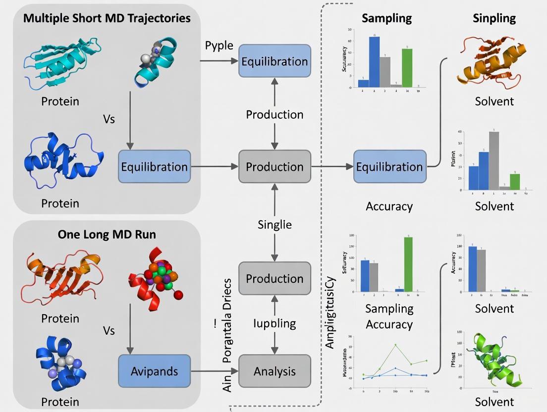
Diagram 2: Workflow for single long run vs. multiple short runs.

The Scientist's Toolkit: Essential Research Reagents and Materials

Table 3: Key Software and Computational Tools for Sampling Studies

Item Name	Function/Description	Application Note
GROMACS	A high-performance MD software package.	Supports both multiple short runs and long simulations. Highly optimized for CPU and GPU computing [1].
NAMD	A parallel MD code designed for high-performance simulation of large biomolecular systems.	Scalable for large complexes; integrates with VMD for visualization and analysis [1].
AMBER	A suite of biomolecular simulation programs.	Includes extensive tools for running MD and analyzing trajectories, particularly popular in drug discovery [1].
PLUMED	An open-source library for free energy calculations in molecular systems.	Essential for implementing enhanced sampling methods like metadynamics; works with GROMACS, NAMD, and AMBER [1].
VMD	Molecular visualization and analysis program.	Used for visualizing trajectories, creating publication-quality images, and analyzing structural and dynamic properties [4].
MDAnalysis	A Python toolkit for the analysis of MD trajectories.	Enables scripting of complex analyses and streamlines the comparison of multiple trajectories [4].
Clenhexerol	Clenhexerol Hydrochloride
NBD-Cl	NBD-Cl|4-Chloro-7-nitrobenzofurazan [99%]

The Ergodicity Assumption and the Limitations of Simulation Timescales

The ergodicity hypothesis is a foundational principle in molecular dynamics (MD) simulations, positing that the time average of a molecular system's properties over a sufficiently long simulation will equal its ensemble average [5]. This assumption underpins the validity of using MD trajectories to predict experimentally observable quantities. However, the computational cost of achieving true ergodicity for complex biomolecular systems is often prohibitive [5] [1]. Biomolecules exhibit rugged energy landscapes with numerous local minima separated by high energy barriers, making it easy for simulations to become trapped in non-representative conformational states [1]. This limitation directly impacts the reliability of simulations in fields like drug development, where accurately characterizing molecular dynamics is crucial. The central question in sampling strategy thus becomes: does one long simulation provide a better approximation of the ergodic condition than multiple shorter, independent trajectories? This Application Note examines the theoretical and practical aspects of this question, providing protocols and analyses to guide effective sampling strategies.

Theoretical Background: The Ergodicity Problem in MD

The formal requirement of ergodicity is that a simulation must be long enough to visit all relevant regions of the conformational space with a probability proportional to their Boltzmann weights. In practice, biomolecular systems often violate this assumption due to their complex, multi-funnel energy landscapes and the limited timescales accessible to simulation [1]. A direct consequence is poor sampling of rare events or slow conformational transitions, which can be critical for biological function, such as in protein folding or ligand unbinding [1].

The problem is exacerbated by the fact that the roughness of the energy landscape means that conventional MD simulations can remain trapped in a local minimum for durations that exceed practical simulation times. This trapping leads to non-ergodic behavior and inaccurate estimates of equilibrium properties [1]. Enhanced sampling methods like replica-exchange molecular dynamics (REMD) and metadynamics were developed specifically to address this issue by facilitating barrier crossing [1]. However, the strategic choice between running a single, long trajectory versus multiple short ones remains a fundamental consideration for any MD project, influencing both the quality of the sampling and the practical allocation of computational resources.

Sampling Strategies: A Comparative Analysis

A critical decision in any MD study is whether to allocate computational resources to a single, long simulation or to distribute them across multiple independent, shorter runs. The optimal choice depends on the specific scientific question and the system's characteristics.

Single Long Trajectory

A single long simulation is the traditional approach. Its primary strength is the ability to model slow, correlated motions and observe the temporal sequence of events, which is vital for studying processes like folding or allosteric communication. However, its major weakness is the high risk of becoming kinetically trapped in a local energy minimum, failing to sample the full conformational landscape [1] [6]. For instance, a long simulation of an RNA aptamer was shown to remain trapped in a specific state depending on its initial configuration [6]. From a practical perspective, a single long run also represents a single point of failure; if the simulation crashes, all progress is lost.

Multiple Short Trajectories

The alternative strategy involves initiating multiple independent simulations from different starting conformations. A key study on an RNA aptamer demonstrated that this approach leads to broader conformational sampling and helps avoid deep local energy minima [6]. By starting from diverse points in conformational space, this method effectively performs a parallel exploration of the energy landscape. It is also more robust, as the failure of one simulation does not compromise the entire set. A potential limitation is that each short trajectory may be unable to cross high energy barriers on its own, potentially missing slow, correlated motions that are accessible to a single long run [6].

Table 1: Comparison of MD Sampling Strategies

Feature	Single Long Trajectory	Multiple Short Trajectories
Sampling Breadth	Risk of being trapped in a single local minimum [6].	Superior for exploring diverse conformational states [6].
Rare Events	Can model slow, correlated motions over time.	Better at capturing some rare events through improved state coverage [6].
Kinetic Information	Preserves temporal sequence and long-timescale kinetics.	Provides ensemble statistics but obscures temporal pathways.
Computational Robustness	Single point of failure.	Fault-tolerant; failure of one run does not lose significant data.
Parallelization	Limited to parallelization within a single simulation.	Ideal for high-throughput computing on distributed systems [7].

Quantitative Assessment of Sampling Performance

Rigorous quantitative evaluation is essential for assessing sampling performance. The study of the NEO2A RNA aptamer, which employed 60 independent 100-ns simulations, provides a framework for this assessment [6]. Key metrics include:

• Potential Energy Distribution: Comparing the potential energy distributions across different groups of simulations helps verify that they are sampling consistent regions of the energy landscape [6].
• Recurrence Quantification Analysis (RQA): This technique analyzes conformational transitions and can reveal whether simulations from different starting points exhibit similar dynamic behaviors and recurrence patterns [6].
• Principal Component Analysis (PCA): Projecting trajectories onto principal components allows for a visual comparison of the conformational space sampled by different sets of simulations, identifying both overlapping and uniquely sampled regions [6].

This multi-faceted analysis confirmed that while simulations from different initial structures sometimes explored distinct areas of conformational space, the collective set of multiple short trajectories achieved sufficient sampling without being hindered by kinetic traps [6].

Enhanced Sampling Techniques

When both long and short conventional MD simulations fail to achieve ergodic sampling, enhanced sampling techniques are necessary. These methods manipulate the system's dynamics or energy landscape to accelerate the exploration of phase space.

Table 2: Overview of Enhanced Sampling Techniques

Method	Principle	Typical Application	Considerations
Replica-Exchange MD (REMD)	Parallel simulations at different temperatures (or Hamiltonians) exchange configurations, promoting barrier crossing [1].	Protein folding, peptide dynamics, studying protein protonation states [1].	Computational cost scales with system size. Efficiency sensitive to maximum temperature choice [1].
Metadynamics	History-dependent bias potential is added to collective variables to discourage revisiting sampled states, effectively "filling" free energy wells [1].	Protein folding, molecular docking, conformational changes, protein-ligand interactions [1].	Requires careful pre-definition of collective variables. Accuracy depends on the dimensionality of these variables [1].
Simulated Annealing	System temperature is gradually decreased from a high value, allowing it to escape local minima and settle into low-energy states [1].	Structure refinement, characterizing highly flexible systems, studying large complexes [1].	Variants like Generalized Simulated Annealing (GSA) can be applied to large systems at a lower computational cost [1].

Experimental Protocols

Protocol for Multiple Independent MD Simulations

This protocol is adapted from a study on RNA aptamer sampling and can be generalized for most biomolecular systems [6].

• Generate Initial Conformational Diversity:

  • For systems with no experimental structure, use de novo 3D structure prediction to generate multiple (e.g., 6) distinct starting configurations [6].
  • For systems with a known structure, diversity can be introduced by:
    • Sampling from an existing long trajectory.
    • Using structures from enhanced sampling methods like REMD.
    • Perturbing the starting coordinates with short, high-temperature simulations.

• System Preparation:

  • Prepare the protein structure: complete missing residues, resolve alternative locations, remove co-crystallized ligands/waters, and protonate at the desired pH, paying special attention to histidine protonation states (HIE, HID, HIP) [7].
  • For protein-ligand complexes, ensure ligand coordinates are aligned with the protein and provide ligands in MOL or SDF format [7].
  • Process the structure using a tool like gmx pdb2gmx to assign hydrogens and write coordinates and a topology in the required format (e.g., GROMACS). Commonly used forcefields include AMBER99SB-ILDN and water models like TIP3P [7].

• Equilibration:

  • For each initial conformation, perform energy minimization.
  • Run equilibration simulations in the NVT and NPT ensembles to stabilize temperature and pressure.

• Production Runs:

  • Launch multiple independent production simulations (e.g., 10 per starting configuration). The length of each run should be sufficient to overcome local barriers around the starting point [6].
  • Utilize a high-throughput automation tool like StreaMD to seamlessly manage and distribute these simulations across multiple servers or a cluster with minimal user intervention [7].

• Sampling Assessment:

  • Employ the quantitative metrics listed in Section 3.3 (Potential Energy Distribution, RQA, PCA) to evaluate convergence and identify any under-sampled regions of the conformational landscape [6].

Workflow for Enhanced Sampling using Metadynamics

• Identify Collective Variables (CVs): Select a small number (1-3) of CVs that best describe the process of interest (e.g., a distance, angle, or root-mean-square deviation) [1].
• Define the Bias: Set parameters for the Gaussian hills (height and width) that will be added to the potential energy surface during the simulation.
• Run the Simulation: As the simulation progresses, the history-dependent bias potential builds up, discouraging the system from returning to previously visited states in the CV space.
• Calculate Free Energy Surface: The accumulated bias potential can be used to estimate the underlying free energy surface as a function of the chosen CVs [1].

Diagram 1: Decision workflow for MD sampling strategies.

The Scientist's Toolkit: Essential Research Reagents and Solutions

Table 3: Key Software Tools for MD Sampling and Analysis

Tool Name	Type	Primary Function	Relevance to Sampling
GROMACS [1] [7]	MD Simulation Software	High-performance MD engine for running simulations.	The core software for executing both long and short trajectories; supports enhanced sampling methods like REMD.
StreaMD [7]	Automation Toolkit	Python-based tool for high-throughput MD simulation setup, execution, and analysis.	Automates the workflow for multiple independent simulations across distributed computing environments, minimizing user expertise required.
CharmmGUI [7]	Web-Based Platform	Generates scripts and input files for MD simulations.	Helps prepare systems for simulation but requires users to manually manage execution and pipeline creation for multiple runs.
OpenMM [7]	MD Simulation Framework	A versatile, hardware-accelerated library for building MD simulation pipelines.	Provides the flexibility to create customized pipelines for both standard and enhanced sampling protocols.
Thidiazuron	Thidiazuron (TDZ)	Thidiazuron is a potent plant growth regulator for research into morphogenesis, defoliation, and tissue culture. This product is For Research Use Only (RUO). Not for personal use.	Bench Chemicals
Proxodolol	Proxodolol	Proxodolol is a dual beta- and alpha-adrenergic receptor antagonist for research. This product is for Research Use Only (RUO), not for human use.	Bench Chemicals

The ergodicity assumption remains a central challenge in molecular dynamics simulations. While a single long trajectory can be valuable for resolving slow, sequential processes, the evidence strongly supports the strategy of multiple short, independent trajectories for achieving broader and more robust conformational sampling, especially for complex systems. This approach effectively parallelizes the exploration of the energy landscape, reducing the risk of kinetic trapping and providing better ensemble statistics. The integration of quantitative assessment metrics and, when necessary, enhanced sampling techniques is crucial for validating sampling adequacy and overcoming significant energy barriers. For researchers in drug development, adopting high-throughput automated tools like StreaMD for multiple independent simulations represents a practical and powerful strategy to generate more reliable and insightful molecular models, thereby strengthening the link between simulation data and biological function.

Molecular dynamics (MD) simulation is a powerful computational method that provides atomic-level insight into the motion and function of biomolecules, playing an increasingly critical role in fundamental research and drug development [8]. A fundamental decision in planning MD studies is the choice of sampling strategy: whether to execute a single, long simulation or to conduct multiple, shorter, independent trajectories. This choice directly impacts the computational resources required, the type of information that can be extracted, and the statistical reliability of the results. Framed within a broader thesis on sampling strategies, this application note delineates the core conceptual and practical differences between these two approaches. It provides a structured comparison and detailed protocols to guide researchers in selecting and implementing the optimal strategy for their specific scientific objectives, such as characterizing equilibrium properties, capturing rare events, or modeling complex biomolecular dynamics.

The choice between multiple short trajectories and a single long run is not merely a technicality but a foundational strategic decision. Each approach explores the conformational space of a biomolecule in a distinct manner, with inherent strengths and limitations. The following table provides a high-level comparison of these two core strategies.

Table 1: Strategic Comparison of Multiple Short vs. Single Long Trajectories

Aspect	Multiple Short Trajectories	Single Long Trajectory
Core Philosophy	Statistical sampling from diverse starting points; an ensemble approach.	Continuous observation of a single pathway; a chronological approach.
Key Advantage	Better coverage of conformational diversity; avoids being trapped in local energy minima; highly parallelizable [9] [6].	Can directly observe temporal sequences and long-timescale correlated motions without model building [10].
Typical Application	Characterizing equilibrium ensembles, defining free energy landscapes, and studying processes with multiple pathways [11] [6].	Studying ordered, sequential processes like folding from a defined state, and calculating time-correlation functions [10].
Parallelization	Embarrassingly parallel: simulations are independent and can be run simultaneously on multiple processors [9].	Sequential: the simulation is one long, continuous calculation, though modern hardware and algorithms can accelerate it [10].
Risk of Sampling Bias	Lower risk of being perpetually trapped in a single non-representative state.	Higher risk; the entire simulation can be biased if the initial structure is atypical or becomes trapped [6].
Convergence Assessment	Can statistically assess convergence by comparing property distributions across independent trajectories [6].	Relies on observing property plateaus over time, which can be misleading if the system is trapped [3].

Quantitative Analysis of Sampling Performance

A critical question is how the sampling performance of multiple independent simulations compares to that of a single long run. Research indicates that for a given total simulation time, multiple shorter runs can provide broader and more efficient exploration of conformational space. A landmark study on an RNA aptamer conducted 60 independent 100-ns simulations (totaling 6 μs) starting from a diverse set of initial structures [6]. The study found that this approach allowed the system to avoid undesirable outcomes, such as being trapped in a local minimum, which was a risk in long simulations starting from a single structure. The multiple trajectories collectively sampled a wider region of the conformational space than a single long trajectory of equivalent length, demonstrating the power of this approach for characterizing structural ensembles [6].

Table 2: Key Findings from a Quantitative Sampling Performance Study [6]

Metric	Finding in Multiple Short Trajectories
System	NEO2A RNA Aptamer (25 nucleotides)
Simulation Setup	60 independent simulations, each 100 ns (total 6 μs)
Initial Conditions	10 conformations derived from each of 6 distinct de novo predicted structures
Primary Outcome	Simulations initiated from different predicted models explored regions not visited by other groups.
Conclusion	Conducting multiple independent simulations using a diverse set of initial structures is a promising approach to achieve sufficient sampling and avoid kinetic traps.

Detailed Protocols for Implementation

Protocol A: Executing and Analyzing Multiple Short Trajectories

This protocol is designed for studies aiming to characterize a thermodynamic ensemble or explore diverse conformational pathways, such as protein unfolding or ligand dissociation [11] [6].

Workflow Diagram: Multiple Short Trajectories

Step-by-Step Instructions:

• System Preparation and Energy Minimization: Begin with an experimentally determined structure or a set of predicted models. Solvate the protein in a water box, add ions to neutralize the system, and perform energy minimization to relieve any steric clashes [6].
• Generate Diverse Initial Conditions: To ensure broad sampling, create variation in the starting structures. This can be achieved by:
  • Using different de novo predicted 3D structures if an experimental structure is unavailable [6].
  • Sampling from an existing long trajectory.
  • Assigning different random seeds for initial velocities.
• High-Temperature Equilibration: For each initial structure, run a short MD simulation at a higher temperature (e.g., 370-500 K). This helps to rapidly explore the local conformational basin and generate distinct starting conformations for the production runs [6] [12].
• Select Starting Snapshots: From each high-temperature equilibration run, select multiple non-consecutive snapshots. These will serve as the initial coordinates for the independent production simulations [6].
• Run Production Simulations: Launch multiple independent MD simulations in parallel. Each simulation should be run under identical conditions (temperature, pressure, force field) but from its unique starting snapshot. The length of each simulation should be sufficient to overcome local energy barriers [9] [6].
• Trajectory Analysis: Analyze each trajectory individually and collectively. Key analyses include:
  • Root-mean-square deviation (RMSD): Monitor the structural drift of each trajectory from a reference structure [11] [3].
  • Clustering: Group structurally similar conformations from all trajectories to identify highly populated states [13].
  • Principal Component Analysis (PCA): Project the high-dimensional conformational data onto its essential degrees of freedom to visualize the sampled space [6].
• Model Building and Property Calculation: Use the combined data to build a Markov State Model (MSM) to understand the kinetics and thermodynamics of state-to-state transitions [12]. Alternatively, calculate ensemble-averaged properties (e.g., radius of gyration, SASA) directly from the pool of conformations generated by all trajectories [11].

Protocol B: Executing and Analyzing a Single Long Trajectory

This protocol is suitable for investigating sequential processes, such as the functional cycle of a protein or folding from a native-like state, where temporal continuity is essential [10].

Workflow Diagram: Single Long Trajectory

Step-by-Step Instructions:

• System Preparation and Energy Minimization: As with Protocol A, begin with a well-prepared and minimized system. A representative starting structure, often an experimental conformation, is critical [10].
• Solvent and Environment Equilibration: Carefully equilibrate the solvent and ions around the fixed protein backbone. This is typically done in two stages: first in the NVT ensemble to stabilize temperature, followed by the NPT ensemble to achieve the correct density and pressure [10].
• Release of Restraints: Gradually release the positional restraints on the protein atoms (backbone followed by side-chains) in a step-wise manner, allowing the protein to relax into its environment.
• Production Simulation: Launch a single, continuous MD simulation. Leverage specialized hardware (e.g., GPUs, ANTON) or highly optimized software to achieve the maximum possible performance and reach microsecond-to-millisecond timescales [10].
• Convergence Monitoring: Continuously monitor key properties to check for stability and convergence. This includes the total and potential energy, RMSD from the initial structure, and secondary structure content. A system is considered equilibrated when these properties fluctuate around a stable average [3].
• Temporal Evolution Analysis: Analyze the trajectory to extract information on the sequence of events.
  • Identify key conformational states and the direct pathways connecting them.
  • Calculate time-correlation functions to understand dynamic relationships between different parts of the protein.
  • Identify the precise order of events, such as the formation of specific contacts during a folding process.

Successful execution of MD sampling strategies relies on a suite of software, force fields, and computational resources. The following table details key components of the modern computational scientist's toolkit.

Table 3: Research Reagent Solutions for Molecular Dynamics Sampling

Category	Item	Function & Application Note
Software Packages	GROMACS, NAMD, AMBER	Core MD engines for performing simulations; offer high performance on GPU hardware and include tools for setup and analysis [1] [8] [10].
Enhanced Sampling	PLUMED	A library for implementing enhanced sampling methods, such as metadynamics, which can be integrated with multiple MD engines to accelerate barrier crossing [1].
Analysis & Modeling	MDTraj, PyEMMA, MSMBuilder	Python libraries for efficient trajectory analysis and the construction of Markov State Models (MSMs) from large sets of simulation data [13].
Force Fields	CHARMM, AMBER, OPLS	Molecular mechanics force fields that define the potential energy function and parameters; choice can influence sampling and outcomes and should be selected based on the system [12].
Specialized Hardware	GPU Clusters, ANTON Supercomputer	Dedicated processing units (GPUs) and specialized supercomputers (ANTON) enable dramatically longer and faster simulations, making microsecond-to-millisecond timescales accessible [10].
Structure Prediction	AlphaFold2, ROSETTA	Tools for generating initial 3D structural models when experimental structures are unavailable, providing starting points for simulations [6].

Integrated and Advanced Strategies

The dichotomy between multiple short and single long trajectories is not absolute. Modern research often employs integrated or advanced strategies that leverage the strengths of both approaches.

Adaptive Sampling: This is a powerful iterative technique that bridges the two core strategies. In adaptive sampling, an initial set of short simulations is run and analyzed to identify under-sampled or strategically important regions of the conformational space. New simulations are then seeded from these regions, and the process repeats. This data-driven approach efficiently directs computational resources to improve sampling of rare events and complex energy landscapes [13].

Combining Simulation with Experiment: To overcome force field inaccuracies and validate sampling, simulations can be integrated with experimental data. For instance, Machine Learning methods can be used to "refine" a Markov State Model (MSM) built from MD simulations by incorporating time-series data from single-molecule FRET experiments. This data assimilation creates a consistent model that agrees with both atomic-level simulation and macroscopic experimental observations [12].

Enhanced Sampling Algorithms: Methods like Replica-Exchange MD (REMD) and Metadynamics are designed to improve sampling efficiency. REMD runs multiple simulations at different temperatures, allowing exchanges that help the system escape local energy minima. Metadynamics applies a history-dependent bias potential along chosen collective variables to "fill up" free energy minima and push the system to explore new regions [1]. These methods can be applied in both single-long and multiple-short frameworks to achieve more comprehensive sampling.

In the field of molecular dynamics (MD) simulations, a fundamental strategic decision researchers face is whether to employ a single long trajectory or multiple short trajectories for conformational sampling. While long simulations aim to observe rare events through continuous sampling, approaches using many short trajectories strategically seeded across conformational space can provide a more efficient means to characterize complex energy landscapes and metastable states [14]. The choice between these strategies necessitates robust, quantitative metrics to evaluate sampling performance, with a focus on conformational diversity and state discovery. Proper evaluation ensures that simulations are not only computationally efficient but also biologically insightful, capturing the dynamic essence of protein function that arises from transitions between conformational states [15]. This application note details the key metrics and protocols for assessing sampling performance within the context of comparing multiple short trajectories against a single long run.

Core Metrics for Evaluating Sampling Performance

Quantifying Conformational Diversity

Conformational diversity measures the breadth of structural states explored during simulation. The metrics in the table below form the foundation for a quantitative assessment of diversity.

Table 1: Key Metrics for Quantifying Conformational Diversity

Metric	Description	Interpretation	Application Context
Root Mean Square Deviation (RMSD)	Measures the average distance between atoms of superimposed structures.	Low values indicate structural similarity; high values suggest diversity. Best used after alignment to a reference.	General use for global structural comparison.
Root Mean Square Fluctuation (RMSF)	Calculates the fluctuation of a residue around its average position.	Identifies flexible regions (e.g., loops, termini) and rigid domains (e.g., secondary structures).	Pinpointing local flexibility and mobile regions.
Radius of Gyration (Rg)	Measures the compactness of a protein structure.	A decreasing trend suggests folding or compaction; an increasing trend suggests unfolding.	Tracking large-scale conformational changes like folding.
Template Modeling (TM) Score	A scale-invariant metric for assessing global structural similarity.	Scores range from 0-1; >0.5 suggests generally the same fold, <0.3 indicates random similarity.	Comparing predicted models to experimental structures [16].

Quantifying State Discovery and Transition Dynamics

Beyond diversity, effective sampling must identify discrete metastable states and the transitions between them.

Table 2: Key Metrics for State Discovery and Transition Analysis

Metric	Description	Interpretation	Application Context
Committor (({p}_{B}))	The probability a trajectory from a given configuration will reach state B before A [17].	The definitive metric for reaction progress. ({p}_{B}=0.5) defines a transition state.	Fundamental for mechanism studies; requires significant sampling.
Markov State Models (MSMs)	A network model built from short trajectories that describes probabilities of transitioning between states.	Enables prediction of long-timescale kinetics from short simulations. Validated by its implied timescales.	Ideal for integrating many short trajectories to model dynamics [14].
Free Energy Landscape	Projects the simulation onto collective variables to visualize stable states (basins) and transition barriers (saddles).	Deep basins are stable states; low-probability regions are transition states or unstable intermediates.	Visualizing and quantifying the entire conformational landscape.

Comparative Workflow: Multiple Short vs. Single Long Trajectories

The following diagram illustrates the conceptual and analytical workflow for comparing the two main sampling strategies.

Protocols for Strategic Sampling and Analysis

Protocol A: Generating an Ensemble with Multiple Short Trajectories

This protocol leverages the Dynamical Galerkin Approximation (DGA) to extract long-timescale information from short trajectory data [14].

• System Preparation:

  • Prepare your protein structure using standard solvation and minimization procedures.
  • Define the states of interest (e.g., reactant 'A' and product 'B') based on structural criteria.

• Strategic Seeding of Trajectories:

  • Use enhanced sampling methods or preliminary short simulations to identify a set of initial configurations (seeds) that span the collective variable (CV) space between states A and B.
  • The goal is not random seeding, but strategic placement to ensure coverage of potential transition pathways.

• Running Short Simulations:

  • Launch a large number (e.g., 50-500) of independent, short MD simulations from the seeded configurations.
  • The trajectory length should be sufficient to capture local dynamics but does not need to observe a full state transition. For the Trp-cage miniprotein, trajectories of only 30 ns were effective [14].

• DGA Analysis for Committor and Rates:

  • Objective: Solve for the committor function and transition statistics without a full MSM.
  • Procedure: a. Choose a set of smooth basis functions that capture variations in your CVs across the sampled data. b. Use the DGA framework to compute the matrix elements of the transition operator from the short-trajectory data. c. Solve the resulting linear equations to approximate the committor function for any configuration in the sampled space. d. Use the committor data to compute reaction rates and the reactive current, which reveals the most probable transition pathways.

Protocol B: Leveraging AlphaFold2 for Conformational Seeding

This protocol uses AlphaFold2 (AF2) to generate diverse starting structures for MD simulations, bypassing the need for extensive experimental structures [16].

• Input and MSA Generation:

  • Input the target protein sequence into the standard AF2 pipeline.
  • Generate a deep Multiple Sequence Alignment (MSA).

• Driving Conformational Diversity:

  • To prevent AF2 from collapsing to a single, dominant conformation, stochastically subsample the deep MSA to a much shallower depth (e.g., 16-128 sequences).
  • Run the AF2 prediction multiple times (e.g., 50 models) with different random subsamples of the MSA.

• Model Selection and Validation:

  • Cluster the resulting models and select representatives based on structural diversity (e.g., using RMSD).
  • Validate the models against any known experimental structures for different states using TM-score. A TM-score >0.9 indicates a highly accurate model [16].
  • These diverse AF2 models can serve as excellent starting points for either a single long simulation or an ensemble of short simulations, as they provide structurally plausible seeds across the conformational landscape.

Protocol C: Assessing Convergence in a Single Long Trajectory

This protocol provides methods to evaluate whether a long simulation has sampled sufficiently to yield reliable equilibrium properties [3].

• Property Selection: Choose a set of properties relevant to your biological question. These can include:

  • Global Properties: RMSD, Rg, total energy.
  • Local Properties: RMSF, specific inter-residue distances, dihedral angles.
  • Kinetic Properties: Implied timescales from an MSM.

• Running Average Analysis:

  • For a property ( A ), calculate the running average ( 〈A〉(t) ) from simulation time 0 to ( t ).
  • Criteria for Convergence: The function ( 〈A〉(t) ) should fluctuate around a stable value with small deviations for a significant portion (e.g., the latter half) of the trajectory. The time at which this plateau begins is the convergence time, ( t_c ).

• Interpretation:

  • Be aware that a system can be in partial equilibrium, where some properties (e.g., local distances) have converged, while others (e.g., transition rates between low-probability states) have not [3].
  • Claims of convergence should always be qualified by stating which properties were assessed.

The Scientist's Toolkit: Research Reagent Solutions

Table 3: Essential Software and Resources for Conformational Sampling Studies

Tool/Resource	Type	Primary Function	Relevance to Sampling Strategy
GROMACS [15]	MD Software	High-performance MD simulation engine.	Core tool for generating both long and short trajectories.
OpenMM [15]	MD Software	GPU-accelerated MD simulation toolkit.	Core tool for generating both long and short trajectories.
DGA Estimators [14]	Analysis Algorithm	Extracts long-timescale kinetics from short trajectories.	Essential for analyzing multiple short-trajectory datasets.
AlphaFold2 [16]	Structure Prediction	Predicts protein structures from sequence.	Generates diverse conformational seeds for simulations.
GPCRmd [15]	Specialized Database	Curated MD trajectories for GPCRs.	Source of validation data and system setups for membrane proteins.
ATLAS [15]	General MD Database	Large-scale database of protein MD simulations.	Provides reference data and benchmarks for simulation studies.
True Reaction Coordinates (tRCs) [17]	Theoretical Concept	Optimal collective variables that determine the committor.	Ideal CVs for guiding enhanced sampling in any strategy.
Manganese chloride	Manganese Chloride|High-Purity Reagent|RUO	High-purity Manganese Chloride (MnCl2) for industrial and biochemical research. For Research Use Only (RUO). Not for human consumption.	Bench Chemicals
Triclopyr	Triclopyr|Herbicide|CAS 55335-06-3	Triclopyr is a systemic, auxin-mimicking herbicide for professional research use only. It is For Research Use Only (RUO), not for personal or agricultural application.	Bench Chemicals

Implementing Multiple Short and Single Long Trajectory Strategies

The fundamental challenge of achieving sufficient sampling of conformational space lies at the heart of molecular dynamics (MD) simulation. Within this context, a critical strategic decision emerges: whether to employ a single, long simulation trajectory or multiple, shorter, independent simulations. This application note frames this debate within a broader thesis on sampling strategies, detailing the protocols and demonstrating the advantages of the multiple-independent-simulation approach for studying biomolecular systems, with a particular focus on aptamers and proteins. Evidence suggests that conducting multiple independent MD runs starting from different initial conditions is a promising approach to enhance equilibrium sampling, as it not only samples more broadly in the conformational space compared to a single long trajectory but also can provide more accurate estimates [6]. This strategy is particularly valuable for characterizing the conformation and dynamics of flexible molecules like RNA aptamers, where small conformational changes can significantly impact function [6].

Core Concept: Multiple Short Trajectories vs. One Long Run

The choice between multiple short trajectories and one long run hinges on the goal of obtaining a statistically representative ensemble of molecular conformations. A single long simulation risks being trapped in a local energy minimum, potentially missing important conformational states. In contrast, multiple independent simulations, initiated from a diverse set of starting structures, actively explore the energy landscape from different regions, mitigating the risk of such kinetic trapping [6].

A key study on an RNA aptamer provides compelling evidence for this approach. Researchers conducted 60 independent MD simulations, each 100 ns in duration, starting from ten different conformations derived from six distinct de novo predicted structures [6]. The analysis revealed that simulations initiated from different predicted models explored regions of conformational space that were not visited by other groups, and long simulations from different initial structures were found to be trapped in different states [6]. This underscores the necessity of using different initial configurations to achieve broad sampling. The approach of multiple short simulations helps avoid the problem of the molecule being trapped in a local minimum, an undesirable outcome that can skew the resulting conformational ensemble [6].

Quantitative Comparison of Sampling Strategies

The table below summarizes the performance outcomes observed in a case study comparing the two sampling strategies for an RNA aptamer [6].

Table 1: Quantitative Outcomes of Sampling Strategies from an RNA Aptamer Study

Sampling Strategy	Number of Simulations	Simulation Length	Key Observation	Advantage
Multiple Independent Simulations	60	100 ns each	Discovered more conformational states; identified under-sampled regions on the energy landscape [6]	Avoids kinetic trapping in local minima; provides broader coverage of conformational space [6]
Single Long Simulation	1	Equivalent aggregate length (e.g., 6 μs)	High risk of being trapped in a single state or a subset of states, leading to a non-representative ensemble [6]	Simpler setup; can better study slow, correlated motions if sampling is sufficient

Detailed Protocol for Multiple Independent Simulations

This section provides a step-by-step methodology for implementing a multiple-independent-simulation strategy, based on established practices [6].

Generation of Diverse Initial Conformations

The first and most critical step is the preparation of a diverse set of initial structures to ensure simulations sample different regions of the energy landscape.

• Structure Source: For a molecule with no experimentally-determined structure, begin with de novo 3D structure prediction. The study on the NEO2A aptamer selected six configurations from prediction with various potential energy values [6].
• Initial Solvent Equilibration: Each of the predicted structures should be energy minimized in solution and then equilibrated with MD simulations at high temperature [6].
• Conformation Selection: From each of the high-temperature equilibration runs, select multiple conformations (e.g., 10) to serve as the initial structures for production runs at ambient temperature [6]. This results in a pool of starting conformations (e.g., 60) that are diverse in both structure and energy.

System Setup and Equilibration

A robust and consistent equilibration protocol is essential for all systems before initiating production simulations.

• Solvation and Ionization: Place the solute in an appropriate periodic box (e.g., dodecahedron) with a solvent model such as TIP3P water. Add ions to neutralize the system's charge and to achieve a physiologically relevant salt concentration.
• Energy Minimization: Perform energy minimization to remove any bad contacts, using a method like steepest descent or conjugate gradient, typically for several thousand steps or until the maximum force falls below a specified threshold (e.g., 1000 kJ/mol/nm). This step is often cycled with gmx grompp and gmx mdrun in GROMACS [18].
• Equilibration MD:
  • NVT Ensemble: Equilibrate the system with position restraints on the heavy atoms of the solute. This allows the solvent and ions to relax around the solute. Run for a sufficient time (e.g., 100-500 ps) until the temperature stabilizes at the target value (e.g., 300 K).
  • NPT Ensemble: Equilibrate the system with position restraints on solute heavy atoms to adjust the density of the solvent. Run until the pressure and density stabilize (e.g., 100-500 ps).

The following workflow diagram outlines the key stages from initial structure preparation to the final production simulations.

Production Simulations and Analysis

• Launch Production Runs: Initiate multiple independent MD simulations (e.g., 60 runs of 100 ns each) from the pool of equilibrated starting conformations, using the same parameters (temperature, pressure, integrator, etc.) for all.
• Assess Sampling Performance: Employ a combination of analysis techniques to evaluate the quality and breadth of sampling:
  • Potential Energy Distribution: Evaluate the distribution for the complete set of simulations to identify under-sampled regions on the energy landscape [6].
  • Recurrence Quantification Analysis (RQA): Use RQA to examine the sampling of conformational transitions and the recurrence rate, which can indicate trapping [6].
  • Principal Component Analysis (PCA): Project structures onto the first few principal components to visualize and compare the conformational regions sampled by different groups of simulations [6]. The expectation is a wide region of conformational space is sampled (global) and a partial overlap between different trajectories is achieved (local) [6].

The Scientist's Toolkit: Research Reagent Solutions

Table 2: Essential Materials and Tools for Multiple Independent MD Simulations

Item / Reagent	Function / Explanation	Example / Note
De Novo Structure Prediction	Generates initial 3D models when experimental structures are unavailable.	Provides the diverse set of starting configurations crucial for the protocol [6].
All-Atom Force Field	Defines the potential energy function and parameters for the molecular system.	AMBER, CHARMM, OPLS-AA. Selection is critical for accurate dynamics [19].
MD Simulation Software	Engine for running energy minimization, equilibration, and production dynamics.	GROMACS [18], AMBER, NAMD, OpenMM.
Solvent Model	Represents the aqueous environment in which the solute is embedded.	TIP3P, SPC/E, TIP4P water models.
Analysis Tools Suite	For processing trajectories and quantifying sampling performance.	Tools for PCA, RQA, RMSD, and potential energy calculation [6].
Ceftaroline fosamil	Ceftaroline Fosamil|Anti-MRSA Cephalosporin for Research	Ceftaroline fosamil is a fifth-generation cephalosporin for research on MRSA and bacterial pneumonia. This product is for Research Use Only.
Arzoxifene	Arzoxifene Hydrochloride	Arzoxifene is a potent benzothiophene SERM for cancer and osteoporosis research. This product is for Research Use Only (RUO). Not for human use.

The strategic decision to employ multiple independent, short simulations over a single long run is justified when the objective is broad exploration of a biomolecule's conformational landscape. This approach directly addresses the problem of kinetic trapping in local energy minima, a common pitfall in MD simulations. The recommended practice is to initiate simulations from a diverse set of initial conformations, often derived from de novo structure prediction, and to rigorously assess convergence using a suite of analytical methods including potential energy distributions, PCA, and RQA. For researchers studying flexible systems like aptamers or intrinsically disordered proteins, this protocol provides a robust framework for achieving sufficient sampling and generating a representative conformational ensemble.

The fundamental challenge of achieving sufficient sampling in molecular dynamics (MD) simulations is a central concern in computational biology and drug development. The conventional approach of employing a single, long simulation trajectory is often hindered by the problem of kinetic trapping, where the simulation becomes stuck in a local minimum of the potential energy landscape, failing to explore other functionally relevant conformational states [6]. This case study examines the alternative sampling strategy of conducting multiple short, independent MD trajectories, demonstrating its efficacy in preventing trapping and enhancing the exploration of conformational space. Framed within a broader thesis on sampling strategies, this analysis provides application notes and detailed protocols for researchers aiming to implement this method, particularly in the context of drug design where understanding a protein's complete conformational ensemble is crucial for identifying allosteric sites and mechanisms.

Theoretical Foundation: Local Minima and Sampling

The Problem of Local Minima in MD Simulations

In MD simulations, a local minimum represents a metastable conformational state that is stable to small perturbations but is not the global minimum on the potential energy landscape. The complex, high-dimensional energy landscape of biomolecules, such as proteins and RNA, is characterized by numerous such local minima, separated by energy barriers of varying heights [6]. When a simulation is kinetically trapped, it samples only a limited region of conformational space, leading to a non-ergodic sample that does not represent the true thermodynamic equilibrium of the system. This can result in biased estimations of key properties, such as binding free energies, conformational populations, and dynamic correlations, ultimately reducing the predictive power of the simulation [6].

Multiple Short Runs vs. One Long Run

The strategy of using multiple short runs, each initiated from a different starting conformation, provides a direct solution to the problem of local minima. While a single long simulation might remain trapped within one large energy basin for its entire duration, a set of independent shorter simulations, starting from diverse points in conformational space, can simultaneously explore multiple basins [6]. This approach offers several key advantages:

• Enhanced Exploration: A single long trajectory might spend a great deal of time exhaustively sampling a local minimum before overcoming a large barrier to a new region. Multiple short runs, by starting from different points, can immediately begin sampling distinct regions of the energy landscape.
• Parallelizability: Independent simulations can be run concurrently on high-performance computing clusters, drastically reducing the wall-clock time required to achieve broad sampling.
• Robustness: The aggregate ensemble from multiple runs is less likely to be biased by a single, unfortunate initial condition that leads to immediate trapping.

Table: Comparative Analysis of Sampling Strategies

Feature	Single Long Trajectory	Multiple Short Trajectories
Risk of Kinetic Trapping	High	Lower
Exploration Speed	Slow for broad exploration	Fast for broad exploration
Computational Efficiency	Less efficient for conformational space coverage	More efficient for conformational space coverage
Error Estimation	Difficult	Possible from between-trajectory variances
Parallelization	Limited	Excellent

Quantitative Data and Analysis

A study on an RNA aptamer provides compelling quantitative evidence for the superiority of the multiple short-run strategy. Researchers conducted 60 independent MD simulations, each 100 ns in duration, starting from ten different conformations derived from six distinct de novo predicted structures [6]. The analysis revealed that simulations initiated from the same predicted model helped avoid local energy minima traps. Furthermore, groups of simulations starting from different predicted models were able to sample unique regions of the principal component space that were not visited by other groups, demonstrating a more comprehensive exploration of the conformational landscape [6].

This approach was also shown to be critical for quantifying differences in conformational ensembles, a common task in structure-function studies. Research on beta-lactamase proteins demonstrated that statistically significant differences between native and mutant pairs could be discerned from relatively short MD trajectories (50-100 ns) using advanced statistical measures, underscoring the utility of multiple replicates for robust comparative analysis [20].

Table: Summary of Key Findings from the RNA Aptamer Case Study [6]

Metric	Finding
System	NEO2A RNA Aptamer (25 nucleotides)
Simulation Setup	60 independent simulations, each 100 ns
Initial Structures	10 conformations from 6 de novo predicted models
Primary Result	Different initial configurations explored non-overlapping regions of conformational space
Recurrence Quantification Analysis	Consistent conformational transitions across groups
Conclusion	Multiple independent simulations avoid kinetic traps and achieve sufficient sampling

Application Notes: Protocols and Workflows

Protocol for Multiple Independent MD Simulations

The following workflow is recommended for setting up and executing a study using multiple short MD trajectories.

Step 1: Generation of Diverse Initial Structures

The success of this strategy hinges on the diversity of the starting conformations.

• For proteins/RNAs with known experimental structures: Use available structures from the PDB. If multiple structures are available, use them all.
• For systems with no known structure: Employ de novo 3D structure prediction tools to generate a set of plausible initial models. For the RNA aptamer study, six configurations were selected from de novo prediction with various potential energy values [6].
• Enhancing Diversity: For each distinct configuration (e.g., each predicted model), generate several conformations by:
  • Performing energy minimization in solution.
  • Running short MD equilibration runs at high temperature.
  • Sampling multiple snapshots from these equilibration runs. The RNA aptamer study used 10 conformations per predicted model [6].

Step 2: System Setup and Equilibrium

For each initial conformation:

• Solvation and Ionization: Place the structure in an appropriate solvent box (e.g., TIP3P water) and add ions to neutralize the system and achieve physiological concentration.
• Energy Minimization: Use steepest descent or conjugate gradient methods to remove bad steric clashes.
• Equilibration:
  • Perform a short NVT simulation to stabilize the temperature.
  • Follow with an NPT simulation to adjust the density and pressure of the system to the target values (e.g., 1 bar).

Step 3: Production Runs

• Launch independent production simulations from each equilibrated starting structure. The simulations should be conducted in parallel.
• The length of each simulation should be sufficient to overcome local barriers surrounding the starting point. A duration of 100 ns is a common starting point for moderate-sized systems [6].
• Ensure consistent simulation parameters (force field, temperature, pressure) across all runs.

Step 4: Analysis and Ensemble Validation

• Convergence Assessment: Use Principal Component Analysis (PCA) to project trajectories from different starting points onto a common set of collective variables. Plot the density of these projections to check for overlap and identify regions sampled uniquely by different groups of simulations [6].
• Recurrence Quantification Analysis (RQA): Use RQA to examine the sampling of conformational transitions and compare the recurrence rates and dependence on initial conformation among different groups of simulations [6].
• Potential Energy Landscape: Plot the potential energy distribution for the entire set of simulations to identify any remaining undersampled regions [6].

Workflow Visualization

Diagram 1: High-level workflow for multiple short run MD strategy.

The Scientist's Toolkit: Essential Research Reagents and Software

Table: Essential Tools for MD Sampling Studies

Tool/Reagent	Type	Function	Availability
GROMACS	MD Software Suite	High-performance simulation engine with integrated analysis tools [21].	Freely available
AMBER	MD Software Suite	Includes AmberTools and PMEMD for simulation and analysis.	Commercial & Free components
MDAnalysis	Python Library	Flexible framework for analyzing MD trajectories; supports multiple file formats [21].	Freely available on GitHub
MDTraj	Python Library	Fast and efficient trajectory analysis; integrates with NumPy/SciPy [21].	Freely available
VMD	Visualization Software	Visualization, animation, and analysis of structures and trajectories [21].	Freely available
CPPTRAJ	Analysis Program	Versatile trajectory analysis tool within AmberTools [21].	Freely available
PLUMED	Enhanced Sampling Plugin	Used for enhanced sampling, free energy calculations, and analysis [21].	Freely available
Methyl tricosanoate	Methyl Tricosanoate|2433-97-8|High-Purity Reference Standard		Bench Chemicals
CP-346086	CP-346086, MF:C26H22F3N5O, MW:477.5 g/mol	Chemical Reagent	Bench Chemicals

This case study establishes that a sampling strategy based on multiple short, independent MD trajectories is a powerful and efficient method for mitigating the risk of kinetic trapping in local energy minima. By leveraging diverse initial structures and the inherent parallelizability of independent runs, researchers can achieve a more comprehensive exploration of a biomolecule's conformational landscape within a practical timeframe. The provided protocols and toolkit offer a clear roadmap for scientists in drug development to implement this strategy, thereby enhancing the reliability of their simulations for tasks ranging from understanding protein function and mutation effects to the structure-based design of novel therapeutics.

Molecular dynamics (MD) simulations provide insights into the dynamic behavior of biomolecules, which is critical for understanding their function. A central question in the field involves sampling strategy: whether to use one long MD trajectory or multiple short trajectories. This choice directly impacts the efficiency and accuracy of calculating experimental observables, such as Nuclear Overhauser Effect (NOE) data, which are crucial for determining 3D molecular structures. This application note explores the MD2NOE software, which calculates NOEs directly from MD trajectories, providing a framework for evaluating different sampling strategies within drug discovery and structural biology.

Theoretical Background: Beyond the Inverse Sixth Power Assumption

Traditional methods for interpreting NOEs in structural biology often rely on the inverse sixth power average of inter-proton distances (( \langle r^{-6} \rangle )). This approach assumes that internal molecular motions and overall molecular reorientation are uncorrelated, which simplifies the relationship between NOE build-up rates and inter-nuclear distances [22] [23]. While valid for rigid molecules, this assumption breaks down for flexible molecules that sample multiple conformational states.

The MD2NOE software addresses this limitation by calculating dipole-dipole correlation functions directly from the MD trajectory, without using the averaged ( r^{-6} ) term as an intermediate [22] [23]. This direct method is particularly crucial for molecules like intrinsically disordered proteins, oligomeric carbohydrates, and single-stranded polynucleotides, where internal motions occur on timescales similar to molecular reorientation, making angular and distance variations inseparable [22]. The core correlation function calculated by MD2NOE is given by:

[ C(\tau)=(dd)^2 \left\langle \frac{1}{r^3(t)} \times Y2^0(\Omega(t)) \times \frac{1}{r^3(t+\tau)} \times Y2^0(\Omega(t+\tau)) \right\rangle_t ]

Where ( dd ) is the dipolar interaction constant, ( r(t) ) is the inter-nuclear distance, and ( Y_2^0 ) are spherical harmonics dependent on the orientation ( \Omega ) of the inter-nuclear vector [22]. This direct approach properly accounts for the complex interplay between internal and overall motion, leading to more accurate NOE predictions for flexible molecular systems.

MD2NOE Software Package and Workflow

Implementation and Architecture

MD2NOE is part of a broader suite of C++ command-line programs designed to evaluate MD trajectories and simulate various NMR observables, including spin-lattice relaxation rates, spin-spin relaxation rates, and 3JHH scalar couplings [22] [23]. The software runs under LINUX operating systems and is publicly available at glycam.org/nmr.

Integrated Workflow Modules

The MD2NOE workflow consists of three integrated modules that transform raw MD data into comparable NOE predictions:

Module 1: Input Processing ingests MD trajectories generated by AMBER simulation software along with associated topology files [22].

Module 2: Trajectory Validation assesses whether the simulation has adequately sampled conformational states and achieved steady-state behavior. This module includes auxiliary tools like "TRAJECTORY," which generates plots and text files showing inter-nuclear distances for selected proton pairs as a function of time, allowing researchers to verify that the simulation has reached a stable equilibrium [22].

Module 3: NOE Calculation computes correlation functions for pairwise dipolar interactions directly from the validated trajectory and incorporates the resulting relaxation parameters into a complete relaxation matrix analysis to generate simulated NOE build-up curves for comparison with experimental data [22] [23].

Sampling Strategy: Multiple Short vs. Single Long Trajectories

The core thesis context of sampling strategy presents a significant methodological consideration when using MD2NOE. Each approach offers distinct advantages for conformational sampling and property calculation.

Table: Comparison of MD Sampling Strategies for NOE Calculation

Feature	Single Long Trajectory	Multiple Short Trajectories
Timescale Sampling	Ideal for processes slower than overall tumbling [22]	Better for rapid local fluctuations [10]
Correlation Function	Directly captures slow motions & complex dynamics [22]	May miss slow conformational transitions
Statistical Independence	Sequential time points are correlated	Independent starting points enhance sampling diversity
Computational Efficiency	Requires continuous long-time access to resources	Can be distributed across multiple processors [10]
Error Assessment	Limited to block averaging approaches	Enables statistical comparison across replicates
System Size Limitation	More challenging for large systems	More accessible for large biomolecular complexes

Enhanced Sampling Techniques

For systems with rough energy landscapes and high energy barriers, enhanced sampling methods can improve the efficiency of both single long and multiple short trajectory approaches:

• Replica-Exchange MD (REMD): Simultaneously runs multiple simulations at different temperatures, allowing exchanges between replicas to overcome energy barriers [1].
• Metadynamics: Adds a history-dependent bias potential to discourage revisiting previously sampled states, effectively "filling free energy wells with computational sand" to encourage exploration of new regions [1].
• Simulated Annealing: Gradually reduces an artificial temperature during simulation, helping the system escape local minima and approach a global minimum configuration [1].

Experimental Protocol: Application to Sucrose

System Setup and Trajectory Generation

The developers of MD2NOE validated their approach using sucrose as a model system, following this detailed protocol:

• Force Field and Solvent Selection:

  • Employ the GLYCAM06 force field (version Glycam06h) for sucrose parameters [22] [23].
  • Use the TIP3P water model for solvation [22] [23].
  • Validate force field selection by comparing calculated and experimental scalar proton-proton J couplings [23].

• Simulation Parameters:

  • Generate trajectories using the pmemd.MPI utility in AMBER 12 [23].
  • Conduct simulations in explicit water with a minimum of 1000 water molecules [23].
  • Ensure trajectory length exceeds 100 nanoseconds to adequately sample sucrose's conformational space [22].

Trajectory Analysis with MD2NOE

• Input Preparation: Provide the AMBER topology and trajectory files to MD2NOE Module 1 [22].

• Trajectory Validation:

  • Use Module 2 to plot distances between key proton pairs (e.g., anomeric proton H1 on glucopyranose and trans-glycosidic protons on fructofuranose) as a function of time [23].
  • Verify the simulation has reached steady-state behavior with no systematic drifts in distances [22].

• NOE Calculation:

  • Module 3 calculates correlation functions for all relevant proton pairs directly from the trajectory [22].
  • The software computes spectral density functions and cross-relaxation rates using the formula: [ \sigma{i,j} = \frac{(dd)^2}{4} \left{ -J{ij}(0) + 6J{ij}(2\omega) \right} ] where ( J{ij} ) is the spectral density function for proton pair (i,j) [22].
  • A complete relaxation matrix analysis generates NOE build-up curves for comparison with experiment [22] [23].

Results and Comparison to Traditional Methods

Application to sucrose revealed "small but significant" differences between NOEs calculated by MD2NOE and those derived using traditional inverse sixth-power averaging [22] [23]. The direct calculation approach of MD2NOE demonstrated that the timescales of internal motion and overall reorientation are not fully separable for sucrose, validating the importance of the direct trajectory analysis method for flexible molecules [23].

Table: Research Reagent Solutions for MD2NOE Experiments

Reagent/Resource	Function in Protocol
AMBER MD Software	Generates input trajectories using validated force fields [22] [23]
GLYCAM06 Force Field	Provides parameters for carbohydrates like sucrose [22] [23]
TIP3P Water Model	Explicit solvent for realistic solvation environment [22] [23]
GPU Computing Resources	Enables microsecond-timescale trajectories [22] [10]
LINUX Operating System	Required platform for running MD2NOE software [22]

MD2NOE represents a significant advancement for calculating NMR observables directly from MD trajectories, avoiding simplifying assumptions that limit traditional approaches. For researchers investigating the debate between single long versus multiple short trajectory sampling strategies, MD2NOE provides a quantitative framework for evaluation. The software enables direct comparison of NOE predictions from different sampling approaches against experimental data, offering insights into which strategy better captures the complex dynamics of flexible biomolecules. As MD simulations continue to reach longer timescales through hardware and software advances, tools like MD2NOE will play an increasingly important role in bridging the gap between simulation and experiment in structural biology and drug discovery.

The identification of novel binding sites is a fundamental challenge in structure-based drug discovery. A significant number of therapeutically relevant proteins have been classified as "undruggable" due to the absence of well-defined, stable binding pockets in their ground-state structures [24] [25]. Cryptic pockets—transient binding sites that are not apparent in static crystal structures but become favorable for ligand binding in the presence of a ligand or through protein dynamics—provide a promising avenue to target these challenging proteins [25]. The discovery of the Switch-II pocket in the KRAS protein, which led to FDA-approved drugs after decades of the target being considered undruggable, stands as a seminal example of the therapeutic potential of cryptic pockets [26].

Conventional molecular docking in structure-based drug discovery is often limited because it typically treats the protein target as a rigid body or allows only limited flexibility near the active site [24]. This approach fails to capture the full spectrum of conformational dynamics essential for cryptic pocket formation. Molecular dynamics (MD) simulations have emerged as a powerful technique for modeling conformational changes in ligand-target complexes, providing a solution to the limitations of rigid docking [24]. The Relaxed Complex Method (RCM) represents a sophisticated computational strategy that synergistically combines the extensive conformational sampling of MD simulations with the binding affinity evaluation of molecular docking to identify ligands that bind to these transient cryptic sites [24].

The Relaxed Complex Method: Core Concept and Workflow

The foundational principle of the Relaxed Complex Method is that a protein exists as an ensemble of interconverting conformations, only some of which may contain a druggable cryptic pocket. Rather than docking ligands into a single, static protein structure, the RCM involves docking into multiple representative snapshots extracted from an MD simulation of the target protein [24]. This approach increases the probability of identifying binding poses and pockets that would be missed using a single structure.

The method was notably applied in the development of the first FDA-approved inhibitor of HIV integrase. Initial MD simulations of the protein revealed significant flexibility in its active site region, providing crucial insights that complemented crystallographic data [24]. The workflow of the RCM, detailed below, systematically leverages protein dynamics for drug discovery.

Workflow Visualization

Quantitative Comparison of Cryptic Pocket Detection Methods

Various computational methods have been developed to address the challenge of cryptic pocket identification. The table below summarizes the key approaches, their underlying principles, and relative advantages.

Table 1: Computational Methods for Cryptic Pocket Discovery

Method	Core Principle	Advantages	Limitations
Relaxed Complex Method (RCM)	Docking into multiple protein conformations sampled from MD simulations [24].	Directly incorporates protein dynamics; can use conventional docking tools.	Computational cost of MD; snapshot selection bias.
Mixed-Solvent MD	MD simulations with organic co-solvents (e.g., phenol, isopropanol) probe potential binding sites [25].	Experimentally validated; can identify very cryptic sites.	Requires careful parameterization; can be system-dependent.
Enhanced Sampling MD	Methods like aMD or weighted ensemble path sampling lower energy barriers to accelerate pocket discovery [24] [26].	More efficient sampling of rare events; automated workflows available [26].	Parameters can be non-trivial to set; may require specialized hardware/software.
AI-Based Methods	Machine learning models trained on structural and dynamic features predict cryptic pockets [25].	Rapid prediction; can screen many structures.	Dependent on training data quality and quantity; "black box" interpretation.

The performance of these methods can be quantified by their success in retrospective and prospective studies. For instance, the weighted ensemble path sampling workflow from OpenEye was successfully applied for a large-scale retrospective prediction of known cryptic pockets and provided a proof-of-concept for the Switch-II pocket in KRAS [26].

Protocols for Key Experiments

Protocol 1: Standard Relaxed Complex Method Workflow

This protocol describes the essential steps for implementing the RCM to identify ligands for cryptic pockets.

Objective: To identify potential small-molecule binders of a cryptic pocket by docking a compound library into an ensemble of protein conformations generated by MD simulation.

Materials:

• Initial Protein Structure: A high-resolution experimental (X-ray, cryo-EM) or predicted (e.g., AlphaFold2) 3D structure of the target protein [24].
• Simulation Software: A molecular dynamics package such as ACEMD, GROMACS, or AMBER [6] [27].
• Force Field: A modern biomolecular force field (e.g., CHARMM22*, AMBER ff19SB) [27].
• Solvated System: The protein solvated in a box of explicit water molecules (e.g., TIP3P) and ionized to physiological concentration [27].
• Compound Library: An ultra-large virtual library of drug-like compounds (e.g., Enamine REAL, NIH SAVI) [24].
• Docking Software: A molecular docking program (e.g., AutoDock Vina, GNINA, GLIDE) [24] [28].

Procedure:

• System Preparation:
  • Prepare the protein structure using a tool like OpenEye Spruce, which performs protonation, assigns charge states, and optimizes the hydrogen-bond network at the desired pH [26].
  • Solvate the protein in a cubic water box with at least 9 Ã… padding from the protein to the box edge. Add ions to neutralize the system and achieve a physiological salt concentration (e.g., 0.15 M NaCl) [27].

• Equilibration:

  • Energy minimize the system to remove steric clashes.
  • Perform a short (e.g., 20 ns) MD simulation in the NPT ensemble with harmonic restraints (e.g., 1.0 kcal/mol/Ų) on protein Cα atoms, gradually releasing them to allow solvent relaxation [27].

• Production MD Simulation:

  • Using the equilibrated system as a starting point, run one or more production MD simulations in the NVT or NPT ensemble. For multiple trajectory strategies, initiate several independent simulations (e.g., 5-10 replicas) from different initial atomic velocities or slightly different starting structures [6].
  • Simulation Length: The required length is system-dependent. For initial cryptic pocket screening, multiple short-to-medium length simulations (e.g., 50-500 ns per replica) are often used to balance sampling and computational cost [6].
  • Save trajectory frames at regular intervals (e.g., every 1-10 ns) for subsequent analysis [27].

• Trajectory Analysis and Clustering:

  • Analyze the combined trajectories for the formation of transient pockets using tools like MDTraj or built-in functions in simulation packages.
  • Calculate the root-mean-square deviation (RMSD) of protein residues and perform clustering (e.g., using k-means or hierarchical clustering) to group structurally similar conformations.
  • Select a set of representative snapshots from the largest clusters for docking. Also, include a few structurally unique outliers that may represent rare states with open cryptic pockets.

• Virtual Screening:

  • Prepare the compound library by generating 3D conformers and optimizing the geometry of each molecule.
  • Dock the entire library into each representative protein snapshot using molecular docking software.
  • Scoring: Score and rank the binding poses for each protein-ligand complex using the docking program's scoring function.

• Hit Identification and Analysis:

  • Cross-compare results across all snapshots. Compounds that consistently show favorable binding scores in specific conformational states are strong candidates.
  • Visually inspect the top-ranking poses to confirm binding location, particularly looking for ligands bound to novel pockets that were not present in the initial structure.
  • Select the most promising hits for experimental validation (e.g., biochemical assays, structural biology).

Protocol 2: Enhanced Sampling with Weighted Ensemble for Cryptic Pockets

For targets where cryptic pocket opening is a rare event, enhanced sampling methods can be more efficient than standard MD.

Objective: To use a path-sampling approach to efficiently generate rare protein conformations with open cryptic pockets.

Materials:

• All materials from Protocol 1.
• Enhanced Sampling Software: Software capable of weighted ensemble sampling, such as OpenEye's Orion floes [26].

Procedure:

• System Preparation: Identical to Protocol 1.
• Ensemble Setup:
  • Define progress coordinates (collective variables) that are expected to correlate with pocket opening, such as the distance between two secondary structure elements or the radius of gyration of a binding site region.
  • Discretize the conformational space into bins based on these progress coordinates.
• Weighted Ensemble Simulation:
  • Run multiple parallel, short trajectories.
  • Periodically check the trajectories. When a trajectory moves into a new bin, it may be split to enhance sampling in that region. Trajectories that merge in the same bin may be combined to maintain computational efficiency.
  • Continue the simulation until a predefined number of pocket-open conformations are sampled or a simulation time limit is reached.
• Analysis and Docking:
  • Extract all unique conformations where a pocket is deemed open.
  • Proceed with virtual screening as described in Steps 5 and 6 of Protocol 1, using this enriched ensemble of pocket-bearing structures.

Table 2: Key Resources for Implementing the Relaxed Complex Method

Category / Name	Description	Function in Research
Datasets & Libraries
mdCATH Dataset [27]	A large-scale MD dataset with simulations for 5,398 protein domains at multiple temperatures.	Benchmarking cryptic pocket detection methods; training machine learning models.
Enamine REAL Database [24]	An ultra-large, commercially available library of make-on-demand compounds (billions of molecules).	Source of diverse, drug-like small molecules for virtual screening.
Software & Tools
ACEMD [27]	A high-performance MD simulation software optimized for GPU hardware.	Running production MD simulations for the Relaxed Complex Method.
Orion Floes [26]	A workflow-based platform that includes tools for protein ensemble sampling and cryptic pocket detection.	Implementing enhanced sampling methods like the weighted ensemble approach.
GNINA [28]	A molecular docking software that utilizes deep learning for scoring protein-ligand poses.	Conducting virtual screening against protein snapshots from MD.
HTMD [27]	A Python library for handling MD simulations and trajectory analysis.	Pre-processing structures, analyzing trajectories, and clustering conformations.
CHARMM22* [27]	A state-of-the-art classical force field for simulating proteins.	Providing the physical model for interatomic interactions during MD simulations.

Integration with Sampling Strategy Research: Multiple Short vs. Long Runs

The user's thesis context on "sampling strategy multiple short MD trajectories vs one long run" is highly relevant to the practical implementation of the Relaxed Complex Method. Evidence from benchmarking studies provides critical guidance:

• Multiple Short Trajectories: Conducting multiple independent simulations starting from different initial conditions is a proven strategy to enhance equilibrium sampling [6]. This approach helps avoid the problem of the simulation being trapped in a single local energy minimum and allows for broader exploration of the conformational landscape. A study on an RNA aptamer concluded that using multiple independent simulations starting from a diverse set of predicted structures is a promising approach to achieve sufficient sampling and avoid trapping [6].
• Single Long Trajectories: While a single long simulation might eventually cross major energy barriers, it risks remaining kinetically trapped in a subset of the conformational space for extended periods, especially if started from a single initial structure [6].
• Practical Performance: For RNA structure refinement, short simulations (10–50 ns) were found to provide modest improvements for high-quality starting models but were rarely beneficial for poor models. Longer simulations (>50 ns) often induced structural drift and reduced model fidelity [29]. This suggests that for the RCM, an effective strategy might involve running multiple independent simulations of moderate length (e.g., 5 replicas of 100 ns each), rather than a single microsecond-long trajectory [6]. This balances the need for broad sampling with computational cost and mitigates the risk of individual trajectories becoming non-productive.

Overcoming Sampling Challenges: Pitfalls and Enhanced Techniques

Identifying and Escaping Kinetic Traps in Long Simulations

Molecular Dynamics (MD) simulations are a powerful technique for studying biological systems at atomic resolution. However, a central challenge limits their application: the sampling problem. Biomolecular systems are characterized by rough energy landscapes with many local minima separated by high-energy barriers [1]. During simulation, the system can become trapped in these local minima—a phenomenon known as a kinetic trap—preventing the exploration of all relevant conformational states within feasible simulation times [1]. This trapping hinders the meaningful characterization of a biomolecule's dynamics and function, as biologically relevant states may remain unvisited [1].

The strategic question of whether to employ multiple short trajectories or a single long simulation is central to addressing this challenge. While long runs theoretically allow for the observation of rare events, they risk having the system trapped in non-functional states for extended periods without sampling a diverse set of configurations [1]. This application note explores enhanced sampling techniques and strategic approaches to identify and escape kinetic traps, with particular emphasis on the emerging paradigm of using multiple short trajectories, especially when combined with machine learning.

Kinetic Traps: Fundamental Concepts and Identification

The Nature of Kinetic Traps

In MD simulations, a kinetic trap refers to a metastable state—a local free energy minimum—from which the system cannot easily escape due to surrounding high free energy barriers (Figure 1). When trapped, the simulation spends a disproportionate amount of time sampling a limited conformational subspace, leading to non-ergodic behavior and biased results [1]. This is particularly problematic for studying large conformational changes essential to biological function, such as those required for catalysis or substrate transport [1].

Identifying Traps in Simulations

Recognizing when a simulation is kinetically trapped is crucial for initiating corrective measures. Key indicators include:

• Convergence Failure: Essential observables (e.g., Radius of Gyration, RMSD) do not converge or exhibit limited fluctuation.
• Limited State Space: The system revisits the same structural motifs without exploring new, distinct conformations.
• Barrier Persistence: The simulation fails to transition between known or expected conformational states within the expected timeframe.

Figure 1. A kinetic trap in a free energy landscape. The simulation becomes stuck in a local minimum, unable to cross the high energy barrier to reach the global minimum (functional state) without enhanced sampling.

Enhanced Sampling Methodologies

Several enhanced sampling algorithms have been developed to address the sampling problem. The table below compares three foundational techniques.

Table 1: Core Enhanced Sampling Techniques for Escaping Kinetic Traps

Method	Core Principle	Key Advantages	Limitations & Considerations
Replica-Exchange MD (REMD) [1]	Parallel simulations run at different temperatures (or Hamiltonians), with periodic exchange of states based on Metropolis criterion.	Efficiently samples conformational space; avoids kinetic traps at low T by leveraging higher T replicas; widely implemented [1].	High computational cost (many replicas); choice of maximum temperature is critical for efficiency [1].
Metadynamics [1]	History-dependent bias potential (e.g., Gaussians) is added along selected Collective Variables (CVs) to discourage revisiting of states.	Actively "fills" free energy wells, forcing exploration; provides an estimate of the free energy surface [1].	Accuracy depends on correct choice of a small number of CVs; bias deposition must be carefully tuned [1].
Simulated Annealing [1]	Artificial temperature is gradually decreased from a high value, allowing the system to cross barriers at high T and settle into a low-energy state.	Conceptually simple; well-suited for finding low-energy states in very flexible systems; lower computational cost than REMD for large systems [1].	Risk of quenching into a local minimum if cooling is too rapid; primarily yields thermodynamic, not dynamic, information [1].

Protocol: Setting Up a Temperature-Based REMD Simulation

This protocol outlines the steps for a typical T-REMD simulation using a package like GROMACS or AMBER.

Objective: Enhance conformational sampling of a protein in explicit solvent by running parallel simulations at different temperatures and allowing state exchanges.

Steps:

• System Preparation: Generate the initial protein structure and solvate it in a water box with ions for neutralization, following standard procedure for your MD package.
• Equilibration: Energy minimize and equilibrate the system at the target temperature (e.g., 300 K) using standard NVT and NPT ensembles.
• Replica Setup: a. Determine Temperature Distribution: Use tools like demux or temperature_generator to create a list of temperatures (e.g., 8-32 replicas) that ensure a sufficient exchange probability (target ~20%). A typical range might be 300 K to 500 K. b. Prepare Replica Inputs: Create input files for each temperature. The system composition and number of atoms must be identical for all replicas.
• REMD Simulation: a. Launch: Initiate the multi-replica simulation using the mdrun -multidir or equivalent command in your MD engine. b. Exchange Attempts: Configure the simulation to attempt exchanges between neighboring replicas at a regular interval (e.g., every 1-2 ps). The exchange is accepted based on the Metropolis criterion using the potential energies of the two replicas [1].
• Analysis: a. Demux Trajectories: After the run, use demux tools to reorder the trajectories, creating a continuous time-series for each temperature from the exchanging replicas. b. Analyze Convergence: Monitor properties like RMSD, radius of gyration, and secondary structure over time for signs of improved sampling compared to a single trajectory.

Protocol: Metadynamics for Free Energy Surface Exploration

Objective: Calculate the free energy surface of a biomolecule as a function of selected Collective Variables (CVs) and escape kinetic traps by biasing the simulation along these CVs.

Steps:

• Select Collective Variables (CVs): Choose 1-2 CVs that describe the process of interest (e.g., a distance, a dihedral angle, or a radius of gyration). The choice is critical and should be based on prior knowledge [1].
• System Preparation: Equilibrate the system as in a standard MD simulation.
• Define Bias Parameters: a. Hill Height/Deposition Rate: Set the initial height (or energy) of the Gaussian hills and the frequency (pace) at which they are added. b. Hill Width: Set the width of the Gaussians in the CV space, which determines the bias resolution.
• Run Metadynamics: Execute the simulation. As the simulation progresses, Gaussians are summed in the visited regions of CV space, discouraging revisiting and pushing the system to explore new areas [1].
• Monitor Convergence: The free energy estimate is constructed from the added bias. The simulation is converged when the free energy surface stops changing significantly with time.
• Analysis: Use the simulation output to plot the reconstructed free energy surface as a function of the chosen CVs and identify the metastable states (minima) and the barriers between them.

The Strategic Choice: Single Long Run vs. Multiple Short Trajectories

The choice between one long trajectory and many short ones depends on the scientific goal and the system's landscape.

Table 2: Strategic Comparison: Single Long Trajectory vs. Multiple Short Trajectories

Feature	Single Long Trajectory	Multiple Short Trajectories
Kinetic Traps	High risk of permanent trapping in a local minimum [1].	Lower risk; independent starts can explore different minima.
Sampling Efficiency	Can be inefficient if trapped; wastes resources on correlated samples.	Potentially more efficient for mapping diverse states, especially with ML analysis [30].
Rare Events	Can, in principle, observe the exact pathway and timing of a rare event.	Statistically captures ensembles of pathways and states, but not their precise natural timing [30].
Ergodicity	May be non-ergodic, failing to visit all relevant states [1].	Improved ergodicity by manually seeding diversity.
ML & Generative Model Compatibility	Provides a continuous, but potentially biased, dataset.	Ideal for training; provides diverse, independent snapshots for models like MDGen [30].

Figure 2. A conceptual comparison of sampling strategies. While a single long run risks permanent trapping, multiple short trajectories initiated from diverse starting points can collectively explore a broader ensemble of states.

The Scientist's Toolkit: Essential Reagents & Software

Table 3: Research Reagent Solutions for Enhanced Sampling Studies

Tool / Reagent	Function / Application
GROMACS [1]	A versatile MD simulation package with high performance and built-in support for methods like REMD and Metadynamics.
AMBER [1]	A suite of biomolecular simulation programs with extensive tools for running REMD and analyzing results.
NAMD [1]	A parallel MD code designed for high-performance simulation of large biomolecular systems, supporting various enhanced methods.
PLUMED	An open-source library for CV analysis and free energy methods, often interfaced with major MD codes for performing Metadynamics.
MSMBuilder	A software package for building Markov State Models (MSMs) from many short MD trajectories to elucidate kinetics and thermodynamics.
OpenMM	A toolkit for high-performance MD simulation that offers flexibility for implementing custom biases and integration with ML models.
MDGen [30]	A generative model of MD trajectories that uses multiple short trajectories for training, enabling tasks like forward simulation and transition path sampling.
Urea-13C,15N2	Urea-13C,15N2 Isotope
Ceramide 3	Ceramide 3 (Ceramide NP)

An Integrated Workflow: Combining Strategies with Machine Learning

A modern, powerful approach involves using enhanced sampling to generate initial data, which then fuels a strategy based on multiple short trajectories analyzed with machine learning.

Figure 3. An integrated workflow that leverages the strengths of both enhanced sampling and multiple short trajectories, augmented by machine learning. Step 1 uses REMD or Metadynamics to rapidly explore the energy landscape and identify key metastable states (Step 2). These states are then used as starting points for many short, unbiased simulations (Step 3). The resulting aggregate data trains a generative model (Step 4), which can then be used to efficiently sample new trajectories and pathways (Step 5), providing a powerful surrogate for the original MD force field [30].

This paradigm shift, facilitated by generative models like MDGen, reframes the role of simulation. Instead of relying on a single, long, potentially trapped trajectory, the goal becomes using many short, focused runs to train a model that can then generate accurate and diverse dynamical ensembles on demand for tasks like forward simulation, transition path sampling, and upsampling [30].

Determining the Optimal Number and Length of Short Trajectories

Molecular dynamics (MD) simulations are a cornerstone of modern computational chemistry and biology, providing atomic-level insights into biomolecular processes. A fundamental challenge in the field is designing efficient sampling strategies, particularly when choosing between single long trajectories and multiple short trajectories [1] [31]. While long simulations are often assumed to provide superior sampling, recent methodological advances demonstrate that carefully designed ensembles of short trajectories can yield statistically rigorous predictions of long-timescale phenomena and equilibrium properties at a fraction of the computational cost [14] [32]. This Application Note provides a structured framework for determining the optimal number and length of short MD trajectories for different research objectives, complete with quantitative guidelines and implementable protocols.

Theoretical Foundation: Why Short Trajectories Can Be Optimal

The Statistical Mechanics of Sampling

The core principle underlying the use of multiple short trajectories lies in statistical mechanics. Molecular properties are calculated as ensemble averages, where the quality of the estimate depends more on the statistical independence of conformations than on the temporal continuity of the trajectory [3]. A key insight is that different molecular properties converge at different rates; local structural properties may reach convergence rapidly, while global conformational transitions or free energy landscapes require more extensive sampling [33] [3].

For a system at equilibrium, the ensemble average of a property A is given by: 〈A〉 = (1/Z) ∫ A(r) exp(-E(r)/kBT) dr

where Z is the conformational partition function [3]. Multiple short trajectories started from diverse initial conditions can provide better coverage of the conformational space Ω than a single long trajectory, which might be trapped in local energy minima [11].

The Dynamical Galerkin Approximation

The Dynamical Galerkin Approximation (DGA) provides a mathematical foundation for predicting long-timescale dynamics from short-trajectory data [14]. By representing chemical kinetic statistics through basis set expansions, DGA enables the calculation of key dynamical statistics – including committor functions and reaction rates – without requiring direct observation of rare transition events. This approach demonstrates that correctly constructed estimators from short trajectories show minimal dependence on lag time in the infinite-basis, infinite-sampling limit [14].

Quantitative Guidelines: When to Use Short vs. Long Trajectories

Table 1: Comparative analysis of sampling strategies for different research objectives

Research Objective	Recommended Strategy	Optimal Short Trajectory Length	Minimum Number of Trajectories	Key Supporting Evidence
Local Equilibrium Properties (e.g., residue fluctuations, solvation shell dynamics)	Multiple short trajectories	100-400 ns	5-10 independent replicates	Power law scaling of mean-square displacement with simulation time [33]
Global Conformational Transitions (e.g., protein folding, domain movements)	Hybrid approach: Short trajectories for committor analysis + enhanced sampling	10-30 ns	Sufficient to cover CV space uniformly	DGA analysis of trp-cage folding with 30ns trajectories [14]
Transport Properties (e.g., thermal conductivity, viscosity)	Multiple short trajectories with cepstral analysis	100-400 ps	1 per Cartesian component (×3)	Thermal conductivity calculation in liquids/solids [32]
Free Energy Landscapes	Multiple short trajectories with enhanced sampling	Dependent on CV relaxation times	Varies with system dimensionality	Metadynamics, REMD protocols [1] [31]
Rare Events (transition paths, kinetic rates)	Multiple short trajectories from transition region	Length to cross transition state	Sufficient to estimate committor	Transition Path Theory with DGA [14]

Table 2: Empirical relationships between simulation time and property convergence

System Type	Empirical Scaling Law	Convergence Time for Local Properties	Convergence Time for Global Properties
Small Proteins (e.g., CV-N, 101 residues)	〈(ΔR)²〉 ∝ t⁰·²⁶ [33]	50-100 ns	>400 ns (incomplete) [33]
Miniproteins (e.g., trp-cage, 20 residues)	Dependent on collective variables	10-30 ns for folding mechanisms [14]	>100 ns for complete landscape
Molecular Fluids (e.g., liquid Hâ‚‚O)	Green-Kubo integrals via cepstral analysis [32]	100-400 ps for thermal conductivity	Not applicable

Experimental Protocols

Protocol 1: DGA for Long-Timescale Predictions from Short Trajectories

Application Scope: Predicting folding mechanisms and reaction rates for biomolecules.

Workflow:

• Trajectory Generation:

  • Generate multiple short trajectories (10-30 ns) seeded from diverse regions of configuration space
  • Use enhanced sampling if necessary to improve configuration space coverage [14]

• Basis Set Construction:

  • Construct smooth basis functions from molecular features (e.g., pairwise distances)
  • Avoid indicator functions; prefer smoothly varying functions for better convergence [14]

• Operator Estimation:

  • Compute the transition operator Tt from short trajectory data
  • Solve for committors and other statistics using Galerkin projection [14]

• Validation:

  • Check convergence with respect to basis set size
  • Verify lag-time independence of estimated quantities [14]

DGA Workflow for Long-Timescale Predictions from Short Trajectories

Protocol 2: Optimal Short Trajectory Design for Property Convergence

Application Scope: Determining when short trajectories provide sufficient sampling for equilibrium properties.

Workflow:

• Pilot Study:

  • Run 5-10 trajectories of increasing length (1 ns, 10 ns, 100 ns)
  • Calculate target properties as function of simulation time [33] [3]

• Convergence Assessment:

  • Compute running averages of key properties
  • Determine when fluctuations fall within acceptable error margins [3]

• Power Law Analysis:

  • Plot mean-square displacement vs. simulation time
  • Fit to power law: 〈(ΔR)²〉 ∝ tᵏ [33]

• Ensemble Design:

  • For converged local properties: Use multiple trajectories of minimum length
  • For unconverged global properties: Consider enhanced sampling or longer trajectories [33] [3]

Workflow for Determining Optimal Short Trajectory Parameters

The Scientist's Toolkit: Research Reagent Solutions

Table 3: Essential computational tools for short trajectory strategies

Tool Category	Specific Methods	Function in Sampling Strategy	Key References
Enhanced Sampling Algorithms	Metadynamics, REMD, Simulated Annealing	Improve configuration space coverage for short trajectories	[1] [31]
Dynamical Analysis Frameworks	Dynamical Galerkin Approximation, Markov State Models	Extract long-timescale statistics from short trajectories	[14]
Convergence Metrics	Running averages, autocorrelation functions, block analysis	Determine when properties have converged	[3]
Collective Variables	Dihedral angles, contact maps, path collective variables	Define relevant subspaces for enhanced sampling	[14] [1]
Spectral Analysis Tools	Cepstral analysis, periodogram estimation	Calculate transport properties from short trajectories	[32]
Pretilachlor	Pretilachlor Herbicide	Pretilachlor is a selective herbicide for research on grass and broadleaf weed control in rice. For Research Use Only. Not for personal or agricultural use.	Bench Chemicals

Case Studies and Validation

Case Study: Trp-Cage Miniprotein Folding

The trp-cage miniprotein serves as an excellent validation case for short trajectory strategies. DGA analysis of multiple 30 ns trajectories (totaling only 30 μs of simulation time) successfully reproduced folding mechanisms and committor functions that agreed with previous studies using much longer continuous trajectories [14]. The key to success was the combination of:

• Short trajectories distributed uniformly throughout collective variable space
• Appropriate basis set construction from smooth functions of molecular features
• Improved estimators for rates and committors with reduced lag-time dependence [14]

Case Study: Thermal Conductivity from Short Simulations

For transport properties like thermal conductivity, traditional Green-Kubo approaches require impractically long simulations. Recent work demonstrates that cepstral analysis of the heat flux power spectrum from single, relatively short trajectories (100-400 ps) can yield accurate thermal conductivities for both fluids and solids [32]. This approach leverages the full sample power spectrum information and optimally reduces noise at zero frequency, where the thermal conductivity is determined.

The optimal number and length of short MD trajectories depends critically on the specific research objectives and molecular properties of interest. For local equilibrium properties and specific kinetic questions, multiple short trajectories often provide superior sampling efficiency compared to single long runs. The protocols and guidelines presented here offer a structured approach to designing efficient sampling strategies that maximize information while minimizing computational cost. As methodology continues to advance, particularly through frameworks like DGA and optimized spectral analysis, the strategic use of short trajectories will become increasingly central to computational molecular research.

Molecular dynamics (MD) simulations provide invaluable atomic-level insights into biological processes, yet their effectiveness is often limited by the sampling problem [34] [1]. Biomolecular systems exhibit rough energy landscapes with many local minima separated by high-energy barriers, causing conventional simulations to remain trapped in metastable states and fail to explore the full conformational space relevant to function [1]. The strategic debate between executing multiple short trajectories versus a single long run centers on how best to overcome these barriers. Enhanced sampling methods, particularly Replica-Exchange MD (REMD) and Metadynamics, offer powerful solutions to this challenge by employing different philosophies to accelerate barrier crossing [35] [1].

This application note details protocols for integrating REMD and Metadynamics, creating a synergistic framework that leverages their complementary strengths. This integrated approach is especially valuable for complex biological questions in drug development, such as characterizing intrinsically disordered proteins (IDPs) [36], studying protein-ligand binding [1], and mapping folding landscapes [1].

Theoretical Foundations and Integrated Framework

Replica-Exchange MD (REMD)

REMD enhances sampling by running multiple parallel simulations (replicas) of the same system at different temperatures. Periodic Monte Carlo-based attempts to exchange configurations between adjacent temperature replicas allow the system to escape deep energy minima at low temperatures by temporarily visiting higher temperatures where barriers are more easily crossed [1]. The method provides a broad, global exploration of the energy landscape without requiring pre-defined reaction coordinates, making it suitable for discovering unknown conformational states [1].

Metadynamics

Metadynamics accelerates the sampling of specific, pre-identified transitions by adding a history-dependent bias potential along selected Collective Variables (CVs) [34] [37]. This bias, typically composed of repulsive Gaussian functions, systematically discourages the system from revisiting sampled states, effectively "filling" free energy minima and driving transitions to new regions [34] [1]. The primary strength of Metadynamics is its ability to efficiently calculate free energy surfaces along the chosen CVs [34].

Synergistic Integration Strategy

Integrating REMD and Metadynamics creates a powerful hybrid approach. REMD provides global exploration across the entire energy landscape, while Metadynamics enables targeted excavation of specific, high-barrier transitions. This synergy is particularly effective when knowledge of the system is partial; REMD can identify potential metastable states, and Metadynamics can then be applied to explore the transitions between them. Furthermore, combining these methods can achieve greater acceleration than either method alone, as demonstrated in recent studies combining Metadynamics with stochastic resetting [37].

Table 1: Comparison of Enhanced Sampling Methods

Feature	REMD	Metadynamics	Integrated Approach
Sampling Philosophy	Global exploration via temperature swaps	Local excavation via bias on CVs	Global landscape exploration with focused barrier crossing
Requirement	Set of temperatures/replicas	Pre-defined Collective Variables (CVs)	Both temperatures and CVs
Output	Thermodynamics at all temperatures	Free energy surface along CVs	High-resolution FES and improved kinetics
Computational Cost	High (many parallel replicas)	Moderate (single, but longer trajectory)	Very High
Ideal Use Case	Unknown landscapes, folding, IDP ensembles [36]	Catalysis, ligand binding, conformational changes [1]	Complex transitions in drug targets [38]

Integrated Application Protocol

This protocol outlines the integration of Well-Tempered Metadynamics with REMD for studying a protein-ligand binding process.

System Setup

• Initial Structure: Obtain the protein-ligand complex structure from a database (e.g., PDB). For the unbound state, manually separate the ligand to a distance of >1.5 nm from the binding pocket.
• Solvation and Ions: Place the system (protein alone for unbound simulations, or complex for bound) in a cubic water box (e.g., TIP3P water model) with a minimum 1.2 nm distance between the protein and box edge. Add ions to neutralize the system and then add salt to a physiological concentration (e.g., 150 mM NaCl).
• Energy Minimization: Minimize the system energy using the steepest descent algorithm until the maximum force is below 1000 kJ/mol/nm.
• Equilibration:
  • Perform a 100 ps NVT equilibration at the target temperature (e.g., 300 K) using a thermostat (e.g., v-rescale).
  • Perform a 100 ps NPT equilibration at the target temperature and pressure (1 bar) using a barostat (e.g., Parrinello-Rahman).

Collective Variable (CV) Selection

The choice of CVs is critical for Metadynamics [34]. For protein-ligand binding, effective CVs include:

• Distance: The distance between the ligand's center of mass and the center of mass of the binding pocket residues.
• Ligand Internal Coordinates: Key dihedral angles within the ligand that are known to change upon binding.
• Protein Cavity: The radius of gyration or number of contacts of the binding pocket residues.

Integrated REMD-Metadynamics Simulation

This step uses the PLUMED plugin [34] coupled with a MD engine like GROMACS or AMBER.

• REMD Setup:

  • Number of Replicas: Typically 24-64, depending on system size and temperature range.
  • Temperature Range: The lowest replica should be the target temperature (e.g., 300 K). The highest temperature should be high enough to ensure rapid conformational changes but not cause denaturation (e.g., 400-500 K). Temperatures can be spaced exponentially.
  • Exchange Attempts: Attempt exchanges between neighboring replicas every 1-2 ps.

• Metadynamics Setup (for relevant replicas):

  • Apply Well-Tempered Metadynamics to the lowest 4-8 replicas to ensure accurate free energy estimation at physiologically relevant temperatures.
  • Gaussian Height: Initial height of 1.0-2.0 kJ/mol.
  • Gaussian Width: Determined by preliminary unbiased runs to ensure CVs fluctuate by roughly 1-2 widths within a metastable state.
  • Deposition Rate: A Gaussian is added every 500-1000 steps (1-2 ps).
  • Bias Factor: A value between 10-60 is typical, which controls how quickly the Gaussian height is reduced.

Diagram 1: Integrated simulation workflow.

Analysis and Validation

• Free Energy Surface (FES): Use the sum_hills utility in PLUMED to reconstruct the FES as a function of the CVs from the Metadynamics simulation [34].
• Convergence: Monitor the FES as a function of simulation time to ensure it has converged. The bias potential should stop growing and only fluctuate.
• Reweighting: Extract unbiased ensemble averages and kinetics from the biased simulation using reweighting techniques [34] [37].
• Experimental Validation: Validate computational predictions with experimental data, such as SAXS for IDP ensembles [36] or binding affinities from assays.

Table 2: Key Parameters for Integrated REMD-Metadynamics

Parameter	Recommended Value	Function
Number of REMD Replicas	24-64	Ensures sufficient acceptance probability for exchanges
Highest Temperature	400-500 K	Enables barrier crossing without denaturation
Gaussian Width (σ)	~1/3 of CV fluctuation	Determines resolution of the FES
Gaussian Deposition Rate	Every 1-2 ps	Balances between smooth FES and computational cost
Bias Factor (Well-Tempered)	10-60	Moderates exploration vs. exploitation

The Scientist's Toolkit

Table 3: Essential Research Reagents and Software

Tool	Function/Description	Example/Note
MD Simulation Engine	Performs the numerical integration of Newton's equations of motion.	GROMACS [39], AMBER [39], NAMD [1], OpenMM
Enhanced Sampling Plugin	Implements advanced sampling algorithms like Metadynamics and REMD.	PLUMED (works with major MD engines) [34]
Collective Variable (CV)	A low-dimensional descriptor of the process of interest.	Distances, angles, dihedrals, coordination numbers [34]
Force Field	A set of empirical parameters describing interatomic interactions.	GROMOS [40], CHARMM, AMBER [39], OPLS-AA
Solvent Model	Represents the aqueous environment in the simulation.	Explicit (TIP3P [39], SPC), Implicit (Generalized Born) [39]
Analysis Suite	Tools for processing trajectory data and calculating properties.	MD analysis tools in GROMACS/AMBER/NAMD, VMD, PyMOL

Concluding Remarks

The integration of REMD and Metadynamics represents a robust strategy for tackling the most challenging sampling problems in biomolecular simulation. By combining REMD's broad exploration with Metadynamics' focused excavation, researchers can achieve a more complete picture of complex energy landscapes, which is crucial for applications in drug development such as optimizing lead compounds and predicting accurate binding modes [38]. This synergistic approach, particularly when augmented with modern extensions like stochastic resetting [37], provides a powerful framework for illuminating biological function and accelerating therapeutic discovery.

Leveraging Machine Learning for Efficient Sampling and Analysis

Application Note: Strategic Sampling for Molecular Dynamics

Core Concept: Multiple Short Trajectories vs. Single Long Runs

The choice between running multiple short Molecular Dynamics (MD) simulations versus a single long trajectory is fundamental in computational research, influencing the efficiency, cost, and biological relevance of the results. Evidence suggests that employing multiple shorter trajectories can be a superior strategy for capturing diverse conformational states and constructing a representative view of a protein's energy landscape, aligning with the "funnel" description of protein folding where numerous pathways lead to similar denatured states [11]. This approach effectively addresses the sampling problem inherent in MD, where biological molecules have rough energy landscapes with many local minima separated by high-energy barriers that can trap conventional simulations in non-relevant conformations [1].

Quantitative Comparison of Sampling Strategies

The table below summarizes the key characteristics and applications of the two primary sampling strategies, synthesizing findings from various studies.

Table 1: Strategic Comparison of Sampling Approaches for Molecular Dynamics Analysis

Feature	Strategy A: Multiple Short Trajectories	Strategy B: Single Long Trajectory
Primary Objective	Characterize diverse pathways and denatured state ensembles; enhance sampling of transitions [11].	Probe deep kinetics and rare events within a single, continuous folding/unfolding pathway.
Computational Efficiency	Highly amenable to parallelization, potentially reducing wall-clock time [41].	Sequential computation, often requiring extensive, uninterrupted resources.
Representativeness of Ensemble	High; better for simulating experiments on large ensembles of molecules and confirming generality of observations [11].	Limited to a single pathway, which may not represent the full ensemble of possible behaviors.
Risk of Non-Ergodicity	Lower; reduces the probability of being trapped in a single non-functional conformational substate [1].	Higher; a single trajectory may become trapped and fail to sample other relevant states.
Key Supporting Evidence	Protein unfolding studies (BPTI, CI2, Barnase) show divergent pathways but similar denatured states [11]. Successful model refinement in CASP using inexpensive short MD simulations [41].	Long simulations can show proteins trapped in non-relevant conformations without returning to the original state [1].

Integration with Machine Learning and Enhanced Sampling

The paradigm of using multiple short runs is powerfully augmented by modern Machine Learning (ML) and enhanced sampling techniques. AI-powered methods, such as Message-Passing Monte Carlo (MPMC), use graph neural networks (GNNs) to generate highly uniform sample points in multidimensional spaces, dramatically boosting simulation accuracy [42]. This addresses a key challenge in MD: insufficient sampling often limits its application. Enhanced sampling methods like Replica-Exchange MD (REMD) and Metadynamics are explicitly designed to overcome energy barriers and sample a broader range of conformational states [1].

Table 2: Machine Learning and Enhanced Sampling Techniques for Efficient Sampling

Technique	Primary Mechanism	Advantages for Sampling
Message-Passing Monte Carlo (MPMC) [42]	Graph Neural Networks (GNNs) allow sample points to "communicate" and self-optimize for uniform distribution.	Generates low-discrepancy points; significantly improves precision in high-dimensional problems (e.g., computational finance).
Replica-Exchange MD (REMD) [1]	Parallel simulations at different temperatures exchange system states, facilitating escape from local energy minima.	Efficient free random walks in temperature/potential energy spaces; widely used for folding studies and free energy landscapes.
Metadynamics [1]	Adds a history-dependent bias potential to "fill" visited free energy wells, discouraging re-sampling of states.	Explores entire free energy landscape; useful for protein folding, conformational changes, and molecular docking.
Adaptive Sampling Strategies [43]	ML models identify the most valuable new data points to simulate, optimizing the training data collection.	Reaches benchmark model performance with fewer data samples; reduces prohibitive computational costs of data generation.

Experimental Protocols

Protocol 1: Multi-Trajectory Analysis of Protein Unfolding

This protocol is adapted from methods used to compare multiple MD simulations of protein unfolding pathways and denatured ensembles [11].

1. System Setup:

• Proteins: Bovine Pancreatic Trypsin Inhibitor (BPTI), Chymotrypsin Inhibitor 2 (CI2), Barnase.
• Software: ENCAD molecular dynamics program.
• Force Field: Levitt et al. force field [11].
• Condition: High-temperature denaturation.

2. Simulation Execution:

• Run multiple independent unfolding simulations (e.g., 11 for BPTI, 4 for CI2) starting from the native state [11].
• Parameters:
  • Time-step: 2 fs.
  • Structures saved every 0.2 ps.
  • Non-bond interactions: 14 Ã… cutoff.

3. Trajectory Analysis:

• Cα Root-Mean-Squared Deviation (RMSD): Calculate the Cα RMSD between structures from different trajectories to assess geometric similarity [11].
• Property-Based Comparison: Monitor time-dependent global and local properties for each trajectory, creating a "property space" pathway. Key properties include:
  • Radius of gyration.
  • Solvent-accessible surface area.
  • Secondary structure content.

4. Data Interpretation:

• Compare the different trajectories both qualitatively and quantitatively.
• Determine if divergent pathways in conformational space still lead to denatured states with similar physical properties [11].

Protocol 2: ML-Enhanced Refinement of Protein Models (CASP-style)

This protocol outlines an MD-based refinement method that uses multiple short trajectories, as successfully employed in CASP12 [41].

1. System Setup:

• Software: CHARMM MD program.
• Force Field: CHARM22/CMAP.
• Solvent Model: FACTS implicit solvent model.
• Initial Structure: Protein model to be refined.

2. Energy Minimization and Equilibration:

• Add hydrogen atoms with the HBUild command.
• Perform 12,100 steps of energy minimization using the Adopted Basis Newton-Raphson (ABNR) method.
• Gradually heat the system from 50K to 298K over 400 ps with weak harmonic restraints (0.05 kcal/mol/Ų) on Cα atoms.

3. Production Runs - Multiple Short Trajectories:

• Short MD (Restrained):
  • Execute sixty independent 1.2 ns simulations.
  • Apply increasing positional restraints on Cα atoms (0.1, 0.2, 0.4 kcal/mol/Ų), changing every 400 ps.
• Long MD (Weakly Restrained):
  • Execute twenty independent 20 ns simulations.
  • Apply weak positional restraints (0.05 kcal/mol/Ų) on Cα atoms.
• General Parameters:
  • Temperature: 298 K.
  • Time-step: 2 fs (bonds involving H constrained with SHAKE).
  • Save structures every 1 ps.

4. Model Selection and Filtering:

• Extract structures from all trajectories (e.g., 72,000 from short MD, 400,000 from long MD).
• For each extracted model, calculate:
  • iGDT_HA: Similarity to the starting model.
  • DFIRE: Statistical knowledge-based potential score.
• Normalize both scores (iGDT_HA, DFIRE) to Z-scores relative to the distribution from each MD trajectory.
• Apply a filter to select models that are both geometrically favorable (low ZDFIRE) and not overly deviated from the start (high ZiGDT_HA), based on a pie-shaped selection criterion in the Z-score plot [41].

5. Generation of Final Refined Model:

• Average the Cartesian coordinates of the selected models.
• Perform a final energy minimization and a short 10 ps MD relaxation on the averaged structure.

Workflow and Pathway Visualizations

Workflow for ML-Augmented Multi-Trajectory Refinement

The following diagram illustrates the integrated protocol for refining protein structures using multiple short MD trajectories guided by machine learning selection.

Diagram Title: ML-Driven Multi-Trajectory Refinement

Sampling Strategy Decision Pathway

This diagram provides a logical flowchart for researchers to decide between a single long trajectory and multiple short trajectories based on their study goals.

Diagram Title: Sampling Strategy Decision Pathway

The Scientist's Toolkit: Essential Research Reagents & Solutions

Table 3: Key Software and Computational Tools for ML-Enhanced MD Sampling

Tool / Resource	Type	Primary Function in Research	Example Use Case
CHARMM [41]	Molecular Dynamics Software	Performs energy minimization, heating, equilibration, and production MD simulations.	Protein structure refinement with implicit solvent models.
ENCAD [11]	Molecular Dynamics Software	Calculates long unfolding simulations and compares multiple trajectories.	Studying protein unfolding pathways and denatured ensembles.
AMBER, GROMACS, NAMD [1]	Molecular Dynamics Software	Popular MD packages with implementations for enhanced sampling algorithms like REMD.	Running replica-exchange simulations to overcome energy barriers.
Graph Neural Networks (GNNs) [42]	Machine Learning Architecture	Enables sample points to "communicate" for generating highly uniform (low-discrepancy) point sets.	Message-Passing Monte Carlo (MPMC) for high-dimensional numerical integration.
Replica-Exchange MD (REMD) [1]	Enhanced Sampling Algorithm	Enhances conformational sampling by exchanging system states between parallel simulations at different temperatures.	Studying free energy landscapes and folding mechanisms of peptides and proteins.
Metadynamics [1]	Enhanced Sampling Algorithm	Improves ergodicity by discouraging re-sampling of previously visited states, effectively "filling" free energy wells.	Exploring conformational changes, protein folding, and ligand-protein interactions.
DFIRE [41]	Statistical Potential	A knowledge-based scoring function used to evaluate the geometric favorability of protein structures.	Filtering and selecting optimal models from MD trajectories during refinement.
CGCNN [43]	Machine Learning Model	Crystal Graph Convolutional Neural Network for predicting material properties; can be trained with adaptive sampling.	Predicting physical properties of materials with reduced training data.

Benchmarking and Choosing Your Strategy: A Comparative Framework

In molecular dynamics (MD) simulations, the choice of sampling strategy—multiple short trajectories versus a single long run—is fundamental and directly influences the interpretation of biomolecular motion and stability. This article provides application notes and protocols for three key quantitative methods used to compare and contrast these strategies: Root-Mean-Square Deviation (RMSD), Principal Component Analysis (PCA), and Recurrence Analysis. Within the context of drug discovery, these methods are indispensable for assessing conformational ensembles, identifying metastable states, and validating the adequacy of sampling for therapeutic targets such as proteins and nucleic acids [44] [45]. The subsequent sections detail the underlying principles, provide comparative data, and offer standardized protocols for their application.

Theoretical Background and Quantitative Comparison

• Root-Mean-Square Deviation (RMSD): RMSD is a standard measure of the average distance between atoms in two superimposed molecular structures. It quantifies the global structural deviation from a reference frame. The formula for calculating the RMSD between two coordinate sets, ( v ) and ( w ), for ( n ) atoms is given by: [ \text{RMSD} = \sqrt{\frac{1}{n} \sum{i=1}^{n} |vi - wi|^2} ] where ( vi ) and ( w_i ) are the coordinates of atom ( i ) in the two structures after optimal alignment [46]. A variant known as moving RMSD (mRMSD) calculates the RMSD between a structure at time ( t ) and a structure at time ( t - \Delta t ), which eliminates the need for a fixed reference structure and is useful for analyzing proteins with unknown native states [46].

• Principal Component Analysis (PCA): PCA, also known as Essential Dynamics, is a multivariate technique that reduces the high dimensionality of MD trajectory data to reveal the most important collective motions. It involves diagonalizing the covariance matrix ( C ) of atomic coordinates (often Cα atoms) [47] [48]. The elements of the covariance matrix are defined as: [ C{ij} = \langle (qi - \langle qi \rangle)(qj - \langle qj \rangle) \rangle ] where ( qi ) and ( q_j ) are mass-weighted Cartesian coordinates, and ( \langle \cdots \rangle ) denotes the average over all trajectory frames [49]. The diagonalization yields eigenvectors (principal components, PCs) that represent the directions of maximal variance, and eigenvalues that correspond to the magnitude of variance along each PC. The first few PCs often describe large-scale, biologically relevant motions [47].

• Recurrence Analysis: While the provided search results lack extensive detail on Recurrence Analysis, it is generally understood in the context of MD as a method to identify when a molecular system revisits a previously sampled conformational state. It often involves constructing a recurrence plot from a time series (e.g., a principal component or RMSD trajectory), where a point is marked at ( (i, j) ) if the states at times ( i ) and ( j ) are similar within a threshold. This can be used to quantify the recurrence of states and identify metastable regions and transition patterns.

Comparative Analysis of Methods

Table 1: Quantitative Comparison of RMSD, PCA, and Recurrence Analysis

Feature	RMSD / mRMSD	Principal Component Analysis (PCA)	Recurrence Analysis
Primary Function	Measures global structural change from a reference [46] [50]	Identifies large-scale, collective motions; reduces dimensionality [47] [48]	Identifies when a system revisits a previous conformational state
Dimensionality	Single scalar value per frame	Multiple components (typically 2-10 used) capturing collective motions [47]	Based on a state-space (often from PCA or RMSD)
Information Revealed	Global stability and convergence; stable state regions [46]	Essential subspace; conformational populations and transitions [51] [49]	Metastability, state recurrence, and transition patterns
Reference Dependency	Requires a reference structure (except mRMSD) [46]	Reference-free; based on variance within the trajectory itself [47]	Self-referential; compares states within the same trajectory
Strengths	Intuitive, easy to compute, good initial stability check [46]	Powerful for revealing functional motions masked in RMSD; filters out high-frequency noise [47] [51] [49]	Directly visualizes temporal state recurrences and metastability
Limitations	Can mask large but correlated motions; single metric can be reductive [51]	Linear method; may miss non-linear motions; interpretation of PCs can be complex [47] [48]	Highly dependent on parameter selection (e.g., distance metric, threshold)

Table 2: Impact of Sampling Strategy on Methodological Outcomes

Aspect	Single Long Trajectory	Multiple Short Trajectories
RMSD Analysis	Can show clear transitions between stable states over time [46]	May only capture local minima or initial relaxation; harder to distinguish from noise
PCA Results	Robust estimation of covariance matrix; well-defined essential subspace [47] [48]	PCA must be performed on a combined trajectory; essential subspace may be poorly defined if starts from similar conformations
Recurrence Plot	Can reveal long-term recurrence patterns and stable states	Useful for assessing reproducibility of initial state recurrence across runs
Kinetic Information	Can infer transition rates and pathways from a single, continuous history	Provides limited kinetic information but can assess sampling from different starting points
Risk of Bias	Risk of being trapped in a single local minimum, giving a biased view of the energy landscape	Reduced risk of trapping, but may miss slow, rare events that connect states

Application Notes for Sampling Strategies

Single Long Trajectory vs. Multiple Short Trajectories

The core thesis of comparing sampling strategies revolves around the trade-off between observing rare events and achieving broad conformational coverage.

• Single Long Trajectory: A long simulation is crucial for capturing slow biological processes, such as large-scale conformational changes and folding events. It allows for the direct observation of transition pathways and kinetic rates between states [46] [48]. PCA performed on a long trajectory typically yields a stable and well-converged essential subspace [47]. The primary risk is that the simulation may become trapped in a single metastable basin, providing a biased view of the overall energy landscape.

• Multiple Short Trajectories: An ensemble of shorter simulations, especially when initiated from different conformations (e.g., from crystal structures, NMR ensembles, or normal modes), can more rapidly explore a broader range of conformational space. This approach is less likely to be confined to a single minimum and is useful for mapping stable states. However, short trajectories may fail to capture the slow, collective motions that connect these states, and the PCA may be noisy or incomplete without pooling the data [49]. A combined analysis is often essential.

Integrated Workflow for Comparative Analysis

The following workflow diagram illustrates a recommended protocol for applying RMSD, PCA, and Recurrence Analysis to compare the two sampling strategies.

Figure 1: A unified workflow for comparing MD sampling strategies using RMSD, PCA, and Recurrence Analysis.

Detailed Experimental Protocols

Protocol 1: Moving RMSD (mRMSD) Analysis

This protocol is adapted from the analysis of Trp-cage and NuG2 protein trajectories [46].

• Trajectory Preparation: Extract and align the trajectory to a reference frame (e.g., the first frame) to remove global rotation and translation. For Cα-RMSD, select only Cα atoms.
• Parameter Selection: Choose the time interval ( \Delta t ) for mRMSD calculation. A study on Trp-cage suggested that ≥20 ns is an appropriate time interval to investigate protein dynamics using mRMSD [46]. Test multiple intervals (e.g., 2, 5, 10, 20, 40 ns).
• Calculation: For each frame at time ( t ), calculate the RMSD using the structure at time ( t - \Delta t ) as the reference. The formula is applied with ( v(t) ) and ( w(t - \Delta t) ).
• Visualization and Interpretation: Plot the mRMSD time series. Stable states are indicated by regions with low mRMSD values (~1 Ã… for Cα atoms in Trp-cage). Compare the mRMSD plot with the conventional RMSD plot and total energy calculations to identify stable and metastable states [46].

Protocol 2: Principal Component Analysis (PCA)

This protocol follows established best practices for essential dynamics [47] [48] [49].

• Trajectory Preparation and Alignment: Superimpose all trajectory frames to a common reference structure (usually the first frame or an average structure) to remove global translations and rotations.
• Covariance Matrix Construction: Calculate the covariance matrix of the atomic coordinates. Typically, Cα atoms are used for a coarse-grained view. The matrix is a 3N × 3N matrix for N atoms.
• Diagonalization: Perform eigenvalue decomposition of the covariance matrix to obtain eigenvectors (principal components) and eigenvalues (variances).
• Dimensionality Reduction: Analyze the scree plot (eigenvalues vs. mode index). Select the top few PCs that capture a significant fraction (e.g., 70-80%) of the total variance. These define the "essential subspace" [47].
• Projection and Clustering: Project the original trajectory onto the selected PCs. This transforms the high-dimensional trajectory into a low-dimensional PC space. The projected data can then be clustered (e.g., using K-means) to identify distinct conformational states [49].
• Visualization: Create 2D or 3D scatter plots of the projections onto the first 2 or 3 PCs. Color the points by simulation time or cluster membership to visualize the exploration of conformational space and transitions between states [51].

Protocol 3: Recurrence Analysis

• State Space Definition: Define the state of the system at each time point. This is often done by using the first few principal components from a PCA, creating a low-dimensional state space vector ( \vec{s}(t) ).
• Distance Matrix Calculation: Compute a distance matrix ( D ) where each element ( D_{ij} ) is the distance between states ( \vec{s}(i) ) and ( \vec{s}(j) ) using a chosen metric (e.g., Euclidean distance).
• Thresholding: Choose a recurrence threshold ( \epsilon ) to define when two states are considered recurrent. The recurrence matrix ( R ) is then defined by: [ R{ij} = \Theta(\epsilon - D{ij}) ] where ( \Theta ) is the Heaviside step function.
• Plotting and Quantification: Visualize the recurrence matrix ( R ) as a recurrence plot. Quantify the plot using measures like recurrence rate, determinism, or entropy to characterize the dynamics and metastability.

The Scientist's Toolkit: Research Reagent Solutions

Table 3: Essential Software and Tools for MD Analysis

Tool Name	Type	Primary Function in Analysis	Key Features / Notes
GROMACS [46]	MD Software Suite	Performing simulations and built-in analysis (RMSD, RMSF, PCA)	Highly optimized for CPU/GPU; includes gmx rms, gmx covar, and gmx anaeig tools.
AMBER [49]	MD Software Suite	Performing simulations and analysis	Includes ptraj and cpptraj for trajectory analysis.
MDAnalysis [51] [52]	Python Library	Trajectory analysis and manipulation (flexible scripting)	Powerful for writing custom analysis scripts (e.g., for Recurrence plots); integrates with Python data science stack.
Bio3D [52]	R Package	Comparative analysis of protein structures and trajectories	Used in Galaxy workflow for PCA, RMSD, RMSF; good for statistical analysis and clustering.
VMD / QwikMD [50]	Visualization & Setup	Trajectory visualization, initial system setup, and basic analysis	QwikMD provides a streamlined GUI for setting up and running simulations in NAMD.
Flare (Cresset) [51]	Commercial Software	GUI-based MD analysis, including PCA and FEP	Integrated environment for visualization and analysis; pyflare allows scripting with MDAnalysis.

Within the broader thesis of comparing sampling strategies—multiple short molecular dynamics (MD) trajectories versus a single long run—the accurate assessment of convergence is paramount. Convergence ensures that the simulation has adequately sampled the biologically relevant conformational space, thus providing reliable data for analysis. This application note details two principal categories of methods for evaluating convergence: monitoring the stability of potential energy and quantifying conformational overlap between trajectory segments. While a single long trajectory is often assumed to provide superior sampling, evidence suggests that aggregated ensembles of shorter, independent simulations can achieve comparable, and sometimes superior, convergence for specific properties by more rapidly decorrelating from the initial configuration [53]. This document provides detailed protocols for implementing these essential convergence diagnostics.

Theoretical Framework and Key Metrics

The fundamental goal of convergence analysis is to determine whether a simulation has sufficiently explored the conformational space relevant to the equilibrium properties of interest. A critical concept is that of partial equilibrium, where some properties may reach their converged values while others have not [54] [3]. Properties that are averages over high-probability regions of conformational space (e.g., root-mean-square deviation (RMSD) of a stable core) may converge relatively quickly. In contrast, properties that depend on infrequent transitions or low-probability conformational states, such as free energies and entropies derived from the partition function, require a much more thorough exploration and thus longer simulation times [54] [3].

Table 1: Key Convergence Metrics and Their Interpretation

Metric Category	Specific Metric	Convergence Indicator	Biological Relevance
Potential Energy & Thermodynamic	Total Potential Energy [54]	Stable running average with small fluctuations	System is energetically stable; not drifting.
	Running Average of Property A, 〈A〉(t) [54] [3]	Plateaus with small fluctuations after a convergence time, t_c	The average value of A (e.g., distance, angle) is reliable.
Conformational Overlap & Similarity	Clustering Ensemble Similarity (CES) [55]	Jensen-Shannon divergence between trajectory windows drops to near zero	Conformational space is being re-sampled, not continuously expanding.
	Dimensionality Reduction Ensemble Similarity (DRES) [55]	Jensen-Shannon divergence between trajectory windows drops to near zero	The overall shape of the projected ensemble is stable.
	Ensemble Comparison via Clustering [56]	Relative populations of structural clusters stabilize between trajectory halves	The probability of visiting different conformational substates is consistent.

Detailed Experimental Protocols

Protocol 1: Convergence via Potential Energy and Property Stability

This protocol assesses convergence by monitoring the stability of global thermodynamic and structural properties over time [54].

Workflow Overview

Procedure Steps

• Trajectory Preparation: Begin with a molecular dynamics trajectory that has completed standard equilibration procedures (energy minimization, heating, and pressurization).
• Property Calculation: For every frame in the trajectory, calculate the property of interest, A. Common choices include:
  • The total potential energy of the biomolecule.
  • The root-mean-square deviation (RMSD) of the protein's Cα atoms relative to a reference structure (e.g., the starting crystal structure or an average structure).
• Running Average Computation: Calculate the running average, 〈A〉(t), which is the average of property A from the start of the trajectory (time 0) up to every time point t.
• Visualization and Analysis: Plot 〈A〉(t) as a function of simulation time. Visually inspect the plot for a convergence time, t_c, after which the function 〈A〉(t) exhibits only small fluctuations around a stable average value. The system can be considered partially equilibrated for this property once it remains in this plateau region for a significant portion of the trajectory [54] [3].

Protocol 2: Convergence via Conformational Overlap

This protocol uses more advanced ensemble comparison techniques to determine if different parts of a trajectory are sampling the same conformational distribution [55] [56].

Workflow Overview

Procedure Steps

• Trajectory Windowing: Split the entire trajectory into a series of consecutive windows. A common approach is to use windows of increasing size (e.g., Window 1: frames 0-100, Window 2: 0-200, Window 3: 0-300, etc.) [55].
• Ensemble Representation (Choose One):
  • A. Clustering-based (CES): For each window, perform clustering (e.g., using K-Means) on the atomic coordinates (typically Cα atoms) to group similar structures. The resulting cluster populations define the conformational ensemble for that window [55] [56].
  • B. Dimensionality Reduction-based (DRES): For each window, project all structures onto a low-dimensional subspace, such as the first two or three principal components from Principal Component Analysis (PCA). The density of points in this subspace defines the ensemble [55].
• Similarity Calculation: Compare the ensemble of an early window (e.g., the first 10 ns) to the ensemble of later, larger windows. The similarity is typically quantified using the Jensen-Shannon divergence, which measures the similarity between two probability distributions. A value of 0 indicates identical ensembles.
• Convergence Assessment: Plot the Jensen-Shannon divergence as a function of the window number or simulation time. Convergence is indicated when the divergence value drops to and remains near zero, signifying that additional simulation time is no longer sampling new conformational regions but is re-sampling the same equilibrium distribution [55].

The Scientist's Toolkit

Table 2: Essential Research Reagents and Software Solutions

Item Name	Function / Application	Implementation Example
MDAnalysis	A Python library for the analysis of MD trajectories; implements both CES and DRES convergence methods.	Used in Protocol 2 to load trajectories, perform clustering/dimensionality reduction, and calculate Jensen-Shannon divergence [55].
Clustering Algorithm (e.g., K-Means)	Groups similar structures from a trajectory into clusters based on a distance metric (e.g., RMSD).	In CES, used to partition the conformational space of each trajectory window into discrete states for population comparison [55] [56].
Dimensionality Reduction (e.g., PCA)	Projects high-dimensional structural data onto a low-dimensional space to simplify ensemble comparison.	In DRES, used to represent the ensemble of each window as a distribution in 2D or 3D principal component space [55].
Jensen-Shannon Divergence	A symmetric and bounded metric for quantifying the similarity between two probability distributions.	The core metric in Protocol 2, calculated to compare the cluster or PC distributions of different trajectory windows [55].
Root-Mean-Square Deviation (RMSD)	Measures the average distance between atoms of superimposed structures.	Serves as a primary metric in Protocol 1 for property stability and as the distance metric for clustering in Protocol 2 [54] [11] [56].

Within the field of molecular dynamics (MD) simulations, a central strategic decision researchers face is the choice between running a single, long simulation or initiating multiple, independent short trajectories. This choice directly impacts the efficiency of computational resource utilization, the statistical robustness of the results, and the ability to sample the conformational landscape of the biomolecule under study. This application note provides a structured comparison of these two sampling strategies, focusing on their throughput, parallelization capabilities, and inherent robustness to kinetic trapping. Aimed at researchers and drug development professionals, this document synthesizes current findings and provides practical protocols to guide the design of MD simulation campaigns.

Comparative Analysis of Sampling Strategies

The table below summarizes the core characteristics of the two primary sampling strategies, highlighting their respective advantages and trade-offs.

Table 1: Comparative analysis of single long versus multiple short MD simulation strategies.

Feature	Single Long Trajectory	Multiple Short Trajectories
Throughput & Hardware	Maximizes performance on single GPU/Node; best for benchmarks like ns/day [57].	High aggregate throughput via massive parallelization; efficient on GPU clusters and cloud environments [6] [57].
Parallelization	Limited to intra-simulation parallelization (e.g., multi-GPU within one node) [58]. Embarrasingly parallel at the simulation level; ideal for high-throughput computing and task farming [6].
Robustness to Trapping	High risk of being trapped in a single local energy minimum for the entire simulation duration [6] [29]. High resilience; different trajectories can escape local minima independently and discover diverse states [6] [11].
Sampling Performance	Excellent for studying specific, long-timescale events and kinetics from a single starting point. Broadly explores conformational space from diverse starting points, improving state discovery [6] [11].
Optimal Use Case	Refining already stable structures [29], studying correlated motions and slow, continuous processes. Initial exploration of conformational landscapes, assessing stability, and mitigating risk of starting-point bias [6] [29].

Visualizing Sampling Strategies and Analysis

The conceptual workflow for implementing and analyzing the multiple short trajectories strategy is outlined below.

Workflow for Multiple Independent MD Simulations

Trajectory Map for Visual Comparison

A novel method for comparing multiple simulations is the use of trajectory maps, which are heatmaps that visualize protein backbone movements over time [59].

Experimental Protocols

Protocol for Multiple Independent Simulations

This protocol is adapted from studies on RNA aptamers, where 60 independent simulations were run from different initial conformations [6].

• System Preparation:

  • Source Diverse Initial Structures: Obtain multiple starting conformations. These can be derived from:
    • Different de novo predicted 3D structures [6].
    • Clusters from an experimental ensemble (e.g., NMR).
    • Snapshots from a prior, short, high-temperature simulation.
  • System Setup: For each structure, perform standard MD setup: solvation, ion addition for neutrality, and energy minimization.

• Equilibration:

  • Independently equilibrate each system. A common strategy is to run simulations at a high temperature (e.g., 350K [60]) for a short period to generate diverse starting conformations for the subsequent production runs.
  • Cool the system to the target temperature (e.g., 300K) and equilibrate in the NPT ensemble.

• Production Simulations:

  • Launch all production runs independently and in parallel. For the RNA aptamer study, each of the 60 simulations was run for 100 ns [6].
  • Critical Setting: To maximize GPU throughput and avoid I/O bottlenecks, set the trajectory saving interval appropriately. Saving frames too frequently can reduce performance by up to 4x [57]. Intervals of 1000-10,000 steps are recommended for optimal GPU utilization [57].

• Analysis:

  • Individual Analysis: Calculate standard metrics (RMSD, Rgyr, RMSF) for each trajectory.
  • Ensemble Analysis: Pool data from all trajectories to compute property distributions (e.g., potential energy). Use recurrence quantification analysis (RQA) and principal component analysis (PCA) to examine conformational transitions and sampling coverage [6].
  • Comparative Analysis: Use methods like trajectory maps [59] to visually compare the stability and dynamics captured in different sets of simulations.

Protocol for a Single Long Simulation

This protocol is typical for classical MD refinement studies, such as those benchmarked in CASP15 for RNA [29].

• System Preparation:

  • Start from a single, high-quality initial model. MD refinement works best for fine-tuning reliable models, not correcting poor ones [29].
  • Perform standard setup: solvation, ion addition, and energy minimization.

• Equilibration:

  • Conduct a thorough equilibration in stages (e.g., NVT followed by NPT) to stabilize temperature and density.

• Production Simulation:

  • Run a single, continuous simulation. The length should be chosen based on the scientific question.
  • Note on Length: For refinement, short simulations (10-50 ns) can provide modest improvements for stable models. Longer simulations (>50 ns) may induce structural drift and reduce fidelity [29].
  • Leverage high-performance GPUs (e.g., L40S, H200) for maximum ns/day throughput [57].

• Analysis:

  • Stability Analysis: Monitor RMSD, Rgyr, and secondary structure content over time to assess stability.
  • Kinetic Analysis: Analyze the trajectory for specific slow events or correlated motions that require a continuous path.

The Scientist's Toolkit

Table 2: Essential research reagents and computational tools for MD sampling studies.

Item	Function/Benefit
GROMACS	Highly optimized MD engine for both CPU and GPU; excellent for benchmarking and production runs on HPC systems [58].
AMBER	Suite of MD programs with specialized force fields (e.g., RNA χOL3); pmemd.cuda is optimized for GPU acceleration [58] [29].
OpenMM	Open-source library for GPU-accelerated MD simulations; high flexibility and used in high-throughput screening studies [57] [60].
WESTPA	Software for weighted ensemble simulations, enabling enhanced sampling of rare events [60].
TrajMap.py	Python script for generating trajectory maps, a novel visualization tool for comparing simulation courses and stability [59].
NVIDIA L40S GPU	Server-grade GPU noted for excellent cost-efficiency for traditional MD workloads [57].
NVIDIA H200 GPU	High-performance GPU ideal for machine learning-enhanced workflows and when raw speed is critical [57].
Hydrogen Mass Repartitioning (HMR)	Technique allowing a 4 fs timestep, speeding up simulations ~1.4x without loss of stability [58].

Within the context of sampling strategy research, a central question is whether an ensemble of multiple short molecular dynamics (MD) trajectories can provide a statistically equivalent or superior representation of a biomolecule's conformational landscape compared to a single long simulation run. This Application Note details rigorous protocols for using experimental Nuclear Magnetic Resonance (NMR) observables, alongside other benchmarks, to validate the physical realism and convergence of MD simulations, with a specific focus on evaluating these distinct sampling approaches. The integration of robust validation is critical, as simulations are increasingly relied upon in critical applications such as drug discovery for identifying druggable sites, validating docking outcomes, and exploring protein conformations [61] [62].

The Sampling Strategy: Multiple Short Trajectories vs. a Single Long Run

The choice between performing multiple short trajectories or a single long run is fundamental, as it directly impacts the efficiency of conformational sampling and the statistical reliability of the results.

Key Considerations for Sampling Strategy

The table below summarizes the core characteristics, advantages, and challenges associated with each sampling strategy.

Table 1: Comparison of MD Sampling Strategies

Feature	Multiple Short Trajectories	Single Long Trajectory
Basic Approach	Launching many independent simulations from different initial conditions [14].	One continuous simulation, often extending to microsecond or millisecond timescales [63].
Primary Advantage	Enhanced parallelization, better exploration of distinct metastable states, and more straightforward error estimation from inter-trajectory variance [14].	Naturally captures slow, correlated motions and precise event sequences without assumptions about state decorrelation.
Statistical Power	Improved ability to estimate uncertainties and assign confidence intervals through ensemble repetition [64].	Relies on the ergodic hypothesis; statistical quality depends on the duration of the single continuous trajectory.
Key Challenge	May miss very slow timescale events that occur beyond the length of any individual short trajectory.	Requires massive, continuous computational resources; can appear "stuck" in long-lived metastable states, leading to poor state space convergence.
Validation Focus	Ensuring the collective ensemble accurately represents the true Boltzmann distribution and that individual trajectories are long enough to be physically meaningful.	Demonstrating that the simulation has achieved convergence and has sampled all relevant conformational states.

Workflow for Comparative Study

The following diagram illustrates a generalized workflow for designing a study to compare these two sampling strategies, culminating in experimental validation.

Core Protocol: Back-Validating MD Sampling with NMR Chemical Shifts

NMR chemical shifts are highly sensitive to local atomic environment and backbone conformation, making them excellent quantitative metrics for validating the structural ensembles generated by MD simulations [65].

Experimental Protocol: Acquiring the 2D ¹³C-¹³C NMR Spectrum

This protocol is adapted from the COMPASS (Comparative, Objective Measurement of Protein Architectures by Scoring Shifts) method [65].

• Objective: To obtain a single, unassigned 2D ¹³C-¹³C NMR spectrum containing backbone and side-chain aliphatic signals for subsequent comparison with MD-derived predictions.
• Sample Requirements: ~10-50 mg of ¹³C,¹⁵N-labeled protein in a suitable buffer. The protein should be monomeric and stable for the duration of data collection.
• Data Collection:
  • Pulse Sequence: Use a 2D NMR experiment that yields exclusively one-bond correlations throughout the aliphatic region. Suitable sequences include:
    • Constant-time, uniform-sign cross-peak correlation spectroscopy (CTUC-COSY) [65].
    • SPC5 sequence with a short mixing time [65].
    • Other dipolar or scalar-based sequences optimized for one-bond transfer.
  • Instrument Time: Typically requires several days to a week of spectrometer time on a high-field instrument for a high-quality signal-to-noise ratio.
• Data Processing and Peak Picking:
  • Process the Free Induction Decay (FID) data (e.g., using NMRPipe) with appropriate apodization and zero-filling.
  • Use an automated peak-picking algorithm (e.g., in Sparky) with a minimum signal-to-noise threshold of 6:1 [65].
  • Filter the peak list to retain only aliphatic correlations (0–80 ppm) that are at least 0.5 ppm away from the diagonal [65].
  • Apply a symmetry filter, retaining only peaks that are observed on both sides of the diagonal within a cutoff of 0.3 ppm [65]. This step is highly effective at removing noise.

Computational Protocol: Predicting NMR Observables from MD Trajectories

• Objective: To generate a predicted 2D ¹³C-¹³C peak list from an MD-derived structural ensemble for direct comparison with the experimental spectrum.
• Input: The ensemble of structures from either multiple short trajectories or a single long run (e.g., snapshots extracted every nanosecond).
• Chemical Shift Prediction:
  • For every snapshot in the ensemble, use a software tool like SHIFTX2 [65] to predict the ¹³C chemical shifts for all aliphatic carbon atoms. SHIFTX2 uses sequence, structure, and dynamics to provide accurate predictions.
  • This produces a list of predicted chemical shifts for each carbon atom in each snapshot.
• Generating the Predicted Peak List:
  • For each snapshot, generate a list of cross-peaks by pairing the predicted chemical shifts of covalently bonded aliphatic carbon atoms (e.g., Cα-Cβ).
  • Combine the cross-peaks from all snapshots in the ensemble to create a single, consolidated predicted peak list that represents the entire simulation.

Validation Protocol: The COMPASS Score

• Objective: To quantitatively score how well an MD-generated structural ensemble agrees with the experimental NMR data, without requiring resonance assignments.
• Procedure:
  • Scoring Algorithm: Use a scoring method based on the modified Hausdorff distance to compare the experimental peak list (from Section 3.1) and the predicted peak list (from Section 3.2) [65].
  • This algorithm measures the degree of overlap between the two sets of peaks in the 2D chemical shift space. A lower score indicates better agreement.
• Interpretation:
  • Compute the COMPASS score for the ensemble from multiple short trajectories and for the ensemble from the single long trajectory.
  • The sampling strategy that produces a structural ensemble with a lower COMPASS score is the one whose average conformation and side-chain packing are more consistent with the experimental NMR data [65].
  • The robustness of the result can be gauged by calculating the score for different subsets of the multiple short trajectories.

Supplementary Validation Benchmarks

While NMR chemical shifts are powerful, a robust validation strategy employs multiple benchmarks.

Protein Folding Kinetics and Committor Analysis

For studies involving folding/unfolding or conformational transitions, long-timescale predictions can be extracted from short trajectories using advanced analysis frameworks like the Dynamical Galerkin Approximation (DGA) [14].

• Protocol:
  • Generate a large number of short trajectories seeded from various points in configuration space.
  • Use DGA to estimate key kinetic statistics like the committor function (the probability a trajectory starting from a given structure will reach one state before another) and reactive currents [14].
  • These values can be used to validate against known experimental pathways or rates. For instance, simulations of the trp-cage miniprotein can be validated by comparing the predicted folding rates and transition state ensemble with experimental measurements [14].

Solvation Free Energy and Box Size Artifacts

Calculations of solvation free energy (ΔG) are a stringent test of a force field's accuracy and the simulation's thermodynamic convergence. It is critical to demonstrate that results are independent of technical artifacts, such as simulation box size.

• Protocol:
  • Calculate the hydration free energy of a small molecule (e.g., anthracene) or a protein (e.g., GB1) using an alchemical free energy method in different box sizes [64].
  • Perform multiple repeats (N >= 20) for each box size to gather sufficient statistics for reliable uncertainty estimation [64].
  • Validation: A well-converged simulation will show no statistically significant trend in ΔG as a function of box size. The apparent "box size effect" reported in some studies is an artifact of insufficient sampling and disappears with adequate repetition and proper uncertainty quantification [64].

The Scientist's Toolkit: Essential Research Reagents and Solutions

Table 2: Key Reagents and Software for MD Validation

Item	Function/Benefit
SHIFTX2	Software for rapid and accurate prediction of protein chemical shifts from structural coordinates; essential for bridging MD and NMR data [65].
GROMACS	A widely used, high-performance MD simulation package suitable for running large ensembles of simulations on high-performance computing (HPC) clusters [62].
AMBER/CHARMM	Comprehensive biomolecular simulation suites including force fields and simulation tools; commonly used for protein systems [62].
COMPASS Framework	A computational method for objectively scoring structural models against an unassigned 2D 13C-13C NMR spectrum [65].
Dynamical Galerkin Approximation (DGA)	A mathematical framework for estimating long-timescale kinetic properties (e.g., committors, rates) from ensembles of short trajectory data [14].
13C/15N-labeled Protein	Essential reagent for collecting high-quality NMR data with required sensitivity and resolution for protein structural studies.
MolProbity	A structure-validation tool that provides steric and geometric quality checks for macromolecular structures, ensuring simulated models are physically realistic [66].
wwPDB Validation Server	A web service that provides comprehensive structure validation reports, useful for checking MD-derived models against experimental restraints [66].

The rigorous validation of molecular dynamics simulations against experimental benchmarks is non-negotiable for producing scientifically credible results. The protocols outlined herein for using NMR chemical shifts, folding kinetics, and thermodynamic quantities provide a robust framework for assessing the performance of different sampling strategies. By applying these methods, researchers can objectively determine whether an ensemble of short trajectories provides a more efficient and statistically powerful path to a converged conformational ensemble compared to a single long simulation, thereby accelerating the reliable use of MD in drug discovery and basic research.

Conclusion

The choice between multiple short trajectories and a single long run is not a one-size-fits-all decision but a strategic one, heavily dependent on the specific biological question and system properties. Multiple short runs excel in broadly exploring conformational space, avoiding kinetic traps, and leveraging modern parallel computing resources, making them ideal for characterizing flexible systems or disordered states. In contrast, a single long trajectory may be necessary to study correlated motions and rare events that occur on timescales longer than the duration of a short run. The future of MD sampling lies in hybrid approaches that intelligently combine these strategies with enhanced sampling methods and machine learning potentials. These integrations promise to dramatically accelerate sampling efficiency and accuracy, ultimately deepening our understanding of molecular mechanisms and powerfully driving forward structure-based drug discovery for challenging therapeutic targets.

References

• 1. Enhanced Sampling Techniques in Molecular Dynamics ... [https://pmc.ncbi.nlm.nih.gov/articles/PMC4339458/]
• 2. How Long Should You Run Molecular Dynamics ... [https://parssilico.com/blogs/67-how-long-should-you-run-molecular-dynamics-simulations-for-drug-design]
• 3. Convergence and equilibrium in molecular dynamics ... [https://www.nature.com/articles/s42004-024-01114-5]
• 4. From complex data to clear insights: visualizing molecular ... [https://pmc.ncbi.nlm.nih.gov/articles/PMC11043564/]
• 5. Challenges and opportunities in connecting simulations with ... [https://pmc.ncbi.nlm.nih.gov/articles/PMC6319911/]
• 6. Sampling Performance of Multiple Independent Molecular ... [https://pmc.ncbi.nlm.nih.gov/articles/PMC7439393/]
• 7. StreaMD: the toolkit for high-throughput molecular dynamics ... [https://jcheminf.biomedcentral.com/articles/10.1186/s13321-024-00918-w]
• 8. Molecular dynamics simulation for all - PMC - PubMed Central [https://pmc.ncbi.nlm.nih.gov/articles/PMC6209097/]
• 9. Multiple Trajectories in the Simulations [https://bio-protocol.org/exchange/minidetail?id=2177602&type=30]
• 10. Long-timescale molecular dynamics simulations of protein ... [https://www.sciencedirect.com/science/article/abs/pii/S0959440X09000372]
• 11. Analysis methods for comparison of multiple molecular ... [https://www.sciencedirect.com/science/article/abs/pii/S0022283699928437]
• 12. Linking time-series of single-molecule experiments with ... [https://elifesciences.org/articles/32668]
• 13. Optimizing adaptive sampling via Policy Ranking [https://arxiv.org/html/2410.15259v1]
• 14. Long-timescale predictions from short-trajectory data [https://pmc.ncbi.nlm.nih.gov/articles/PMC8903024/]
• 15. Beyond static structures: protein dynamic conformations ... [https://pmc.ncbi.nlm.nih.gov/articles/PMC12262120/]
• 16. Sampling alternative conformational states of transporters ... [https://elifesciences.org/articles/75751]
• 17. Enhanced sampling of protein conformational changes via ... [https://www.nature.com/articles/s41467-025-55983-y]
• 18. Flow Chart - GROMACS 2025.3 documentation [https://manual.gromacs.org/current/user-guide/flow.html]
• 19. What is the procedure to develop a new force field ... [https://mattermodeling.stackexchange.com/questions/11024/what-is-the-procedure-to-develop-a-new-force-field-for-molecular-simulation]
• 20. Statistical Measures to Quantify Similarity between Molecular Dynamics Simulation Trajectories - PMC [https://pmc.ncbi.nlm.nih.gov/articles/PMC6258182/]
• 21. List of widely used MD Simulation Analysis Tools. [https://bioinformaticsreview.com/20240729/list-of-widely-used-md-simulation-analysis-tools/]
• 22. Direct NOE Simulation from Long MD Trajectories - PMC [https://pmc.ncbi.nlm.nih.gov/articles/PMC4818662/]
• 23. Direct NOE simulation from long MD trajectories [https://www.sciencedirect.com/science/article/abs/pii/S109078071600046X]
• 24. Structure and dynamics in drug discovery [https://www.nature.com/articles/s44386-024-00001-2]
• 25. Computational advances in discovering cryptic pockets for ... [https://pubmed.ncbi.nlm.nih.gov/39778412/]
• 26. miniWebinar: Opening up the druggable universe one ... [https://www.eyesopen.com/webinars/recordings/cryptic-pockets-jan-2025]
• 27. mdCATH: A Large-Scale MD Dataset for Data-Driven ... [https://www.nature.com/articles/s41597-024-04140-z]
• 28. A beginner's approach to deep learning applied to VS and MD ... [https://jcheminf.biomedcentral.com/articles/10.1186/s13321-025-00985-7]
• 29. When Does Molecular Dynamics Improve RNA Models ... [https://www.sciencedirect.com/science/article/pii/S2001037025004040]
• 30. Generative Modeling of Molecular Dynamics Trajectories [https://arxiv.org/html/2409.17808v1]
• 31. Enhanced Sampling Methods for Molecular Dynamics ... [https://livecomsjournal.org/index.php/livecoms/article/view/v4i1e1583]
• 32. Accurate thermal conductivities from optimally short ... [https://www.nature.com/articles/s41598-017-15843-2]
• 33. Longer simulations sample larger subspaces ... [https://pmc.ncbi.nlm.nih.gov/articles/PMC3290687/]
• 34. An Introduction to Enhanced Sampling and Metadynamics [https://www.compchems.com/an-introduction-to-enhanced-sampling-and-metadynamics/]
• 35. Enhanced Sampling in Molecular Dynamics Using ... [https://www.mdpi.com/1099-4300/16/1/163]
• 36. Use of AI-methods over MD simulations in the sampling ... [https://www.frontiersin.org/journals/molecular-biosciences/articles/10.3389/fmolb.2025.1542267/full]
• 37. Combining stochastic resetting with Metadynamics to ... [https://www.nature.com/articles/s41467-023-44528-w]
• 38. Advancing drug development with “Fit-for-Purpose” modeling ... [https://pmc.ncbi.nlm.nih.gov/articles/PMC12436579/]
• 39. Comparison of the conformational dynamics of an N-glycan ... [https://www.sciencedirect.com/science/article/abs/pii/S0008621522002014]
• 40. Machine learning analysis of molecular dynamics ... [https://www.nature.com/articles/s41598-025-11392-1]
• 41. Protein Structure Model Refinement in CASP12 Using ... [https://pmc.ncbi.nlm.nih.gov/articles/PMC5820213/]
• 42. How AI is improving simulations with smarter sampling ... [https://news.mit.edu/2024/how-ai-improving-simulations-smarter-sampling-techniques-1002]
• 43. Sampling strategies to efficiently train machine learning ... [https://www.sciencedirect.com/science/article/pii/S0927025623001611]
• 44. Computational Methods in Drug Discovery - PMC [https://pmc.ncbi.nlm.nih.gov/articles/PMC3880464/]
• 45. Application of computational methods in the drug discovery ... [https://www.sciencedirect.com/science/article/pii/S2211383525005179]
• 46. Analysis of Protein Folding Simulation with Moving Root Mean ... [https://pmc.ncbi.nlm.nih.gov/articles/PMC10015464/]
• 47. Principal Component Analysis: A Method for Determining ... [https://pmc.ncbi.nlm.nih.gov/articles/PMC4676806/]
• 48. A Review of its Application on Molecular Dynamics Data [https://www.sciencedirect.com/science/article/abs/pii/S1574140006020135]
• 49. Principal component and clustering analysis on molecular ... [https://pmc.ncbi.nlm.nih.gov/articles/PMC3592554/]
• 50. | PPT Md simulation [https://www.slideshare.net/slideshow/md-simulation-233070539/233070539]
• 51. Protein Dynamics and Drug Discovery: elevate your project ... [https://cresset-group.com/science/science-resources/drug-discovery-principal-component-analysis/]
• 52. Hands-on: Analysis of molecular dynamics simulations / Analysis of... [https://training.galaxyproject.org/training-material/topics/computational-chemistry/tutorials/analysis-md-simulations/tutorial.html]
• 53. Convergence and reproducibility in molecular dynamics ... [https://www.sciencedirect.com/science/article/pii/S0304416514003092]
• 54. Convergence and equilibrium in molecular dynamics ... [https://pmc.ncbi.nlm.nih.gov/articles/PMC10850365/]
• 55. Evaluating convergence [https://userguide.mdanalysis.org/1.1.1/examples/analysis/trajectory_similarity/convergence.html]
• 56. Ensemble-Based Convergence Analysis of Biomolecular ... [https://pmc.ncbi.nlm.nih.gov/articles/PMC1479051/]
• 57. Benchmarking GPUs for MD Simulations [https://www.linkedin.com/pulse/benchmarking-gpus-md-simulations-speed-cost-insights-barbosa-farias-ynoke]
• 58. Running Molecular Dynamics on Alliance clusters with AMBER [https://computecanada.github.io/molmodsim-amber-md-lesson/26-MD_Software_Benchmarks/index.html]
• 59. Trajectory maps: molecular dynamics visualization and ... [https://pmc.ncbi.nlm.nih.gov/articles/PMC10789246/]
• 60. A Standardized Benchmark for Machine-Learned ... [https://arxiv.org/html/2510.17187v1]
• 61. Applications of Molecular Dynamics Simulations in Drug ... [https://pubmed.ncbi.nlm.nih.gov/37676596/]
• 62. Molecular Dynamics Simulations in Drug Discovery and ... [https://www.mdpi.com/2227-9717/9/1/71]
• 63. Best Practices for Foundations in Molecular Simulations ... [https://pmc.ncbi.nlm.nih.gov/articles/PMC6884151/]
• 64. On the importance of statistics in molecular simulations for ... [https://elifesciences.org/articles/57589]
• 65. Experimental Protein Structure Verification by Scoring with ... [https://pmc.ncbi.nlm.nih.gov/articles/PMC4786943/]
• 66. User guide to the wwPDB NMR validation reports [http://www.wwpdb.org/validation/NMRValidationReportHelp]